Bernhard Holzer, DESY-HERA

IntroductionIntroduction to to TransverseTransverse BeamBeam OpticsOptics

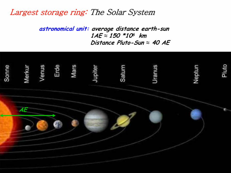
LargestLargest storagestorage ring:ring: TheThe Solar SystemSolar System

astronomical unit: average distance earth-sun1AE ≈ 150 *106 kmDistance Pluto-Sun ≈ 40 AE

AE

HERA Storage Ring: Protons accelerated and stored for 12 hoursdistance of particles travelling at about v ≈ cL = 1010-1011 km

... several times Sun - Pluto and back

LuminosityLuminosity Run of a Run of a typicaltypical storagestorage ring:ring:

guide the particles on a well defined orbit („design orbit“)focus the particles to keep each single particle trajectorywithin the vacuum chamber of the storage ring, i.e. close to the design orbit.

Lorentz force * ( )= + ×r r rrF q E v B

„ ... in the end and after all it should be a kind of circular machine“need transverse deflecting force

typical velocity in high energy machines: 83*10≈ ≈ msv c

old greek dictum of wisdom:if you are clever, you use magnetic fields in an accelerator whereverit is possible.

But remember: magn. fields act allways perpendicular to the velocity of the particleonly bending forces, no „beam acceleration“

TransverseTransverse BeamBeam Dynamics:Dynamics:

0.) Introduction and Basic Ideas

circular coordinate system

* *LF e v B=

condition for circular orbit:

20

Zentrm vF γρ

=

Lorentz force

centrifugal force

20 * *m v e v Bγρ

=

The ideal circular orbit

*p Be

ρ=

ρ

s

θ

z

●

field map of a storage ring dipole magnet

ρ

α

ds0

0 =nIB

hμ

/ *p e B ρ=Normalise to momentum:

... remember

[ ][ ]

01 01 0.2998/

− ⋅⎡ ⎤ = =⎣ ⎦B Te Bm

p p GeV cρ

Magnetic field of a dipole magnet:

„radius of curvature, bending strength“

I.) I.) TheThe MagneticMagnetic Guide Guide FieldField

Dipole Magnets:

define the ideal orbithomogeneous field created by two flat pole shoes

court. K. Wille

required: focusing forces to keep trajectories in vicinity of the ideal orbitlinear increasing Lorentz forcelinear increasing magnetic field = − ⋅ = − ⋅z xB g x B g z

at the location of the particle trajectory: no iron, no current

0∇× = → = −∇r r r r

B B V

the magnetic field can beexpressed as gradient of a scalar potential !

( , ) = ⋅V x z g xz

equipotential lines (i.e. the surface of the iron contour) = hyperbolas

Quadrupole Magnets:

Example:heavy ion storage ring TSR

Calculation of the Quadrupole Field:

normalised quadrupole strength:

gradient of a quadrupole field:

g k/

=p e

Separate Function Machines:

Split the magnets and optimisethem according to their job:

bending, focusing etc

INadjsdHA

*==∫ ∫rrrr

rgrB *)( =

202

rnIg μ

=

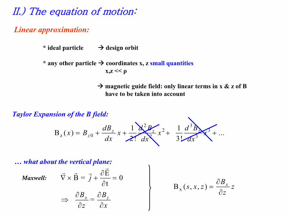
II.) II.) TheThe equationequation of of motionmotion::

Linear approximation:

* ideal particle design orbit

* any other particle coordinates x, z small quantitiesx,z << ρ

magnetic guide field: only linear terms in x & z of B have to be taken into account

Taylor Expansion of the B field:2 3

2 3z 0 2 3

1 1 B ( ) ...2! 3!

= + + + +z z zz

dB d B d Bx B x x xdx dx dx

… what about the vertical plane:

Maxwell:E B = 0t

∂∇ × + =

∂

rr r r

j

=∂ ∂⇒

∂ ∂x zB B

z x

x B ( , , ) ∂=

∂xBs x z z

z

Equation of Motion:

●

z

x

ρ

s

θ

z

●Consider local segment of a particle trajectory... and remember the old days:(Goldstein page 27)

radial acceleration:

22

2⎛ ⎞= − ⎜ ⎟⎝ ⎠

rd da

dtdtρ θρ Ideal orbit: , 0= =

dconstdtρρ

Force:2

2⎛ ⎞= =⎜ ⎟⎝ ⎠

dF m mdtθρ ρω

2 /=F mv ρgeneral trajectory:

2 2

2 ( )= + − =+ z

d mvF m x eB vxdt

ρρ

develop for small x:2 2

2 (1 )− − = zd x mv xm eB vdt ρ ρ

x ρ<<

guide field in linear approx.

0∂

= +∂

zz

BB B xx

2 2

02 (1 ) ∂⎧ ⎫− − = +⎨ ⎬∂⎩ ⎭zBd x mv xm ev B x

xdt ρ ρ

independent variable: t → s

′ = dxx ds

*=dx dx dsdt ds dt

01 (1 ) eBx exgxmv mvρ ρ

′′ − − = +

21 1′′ − + = − +

xx kxρ ρρ

21( ) 0′′ + − =x x kρ

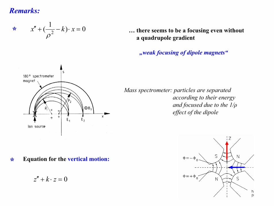
Remarks:

21( ) 0′′ + − ⋅ =x k xρ

… there seems to be a focusing even withouta quadrupole gradient

„weak focusing of dipole magnets“

Mass spectrometer: particles are separatedaccording to their energyand focused due to the 1/ρeffect of the dipole

Equation for the vertical motion:

0′′ + ⋅ =z k z

*

*

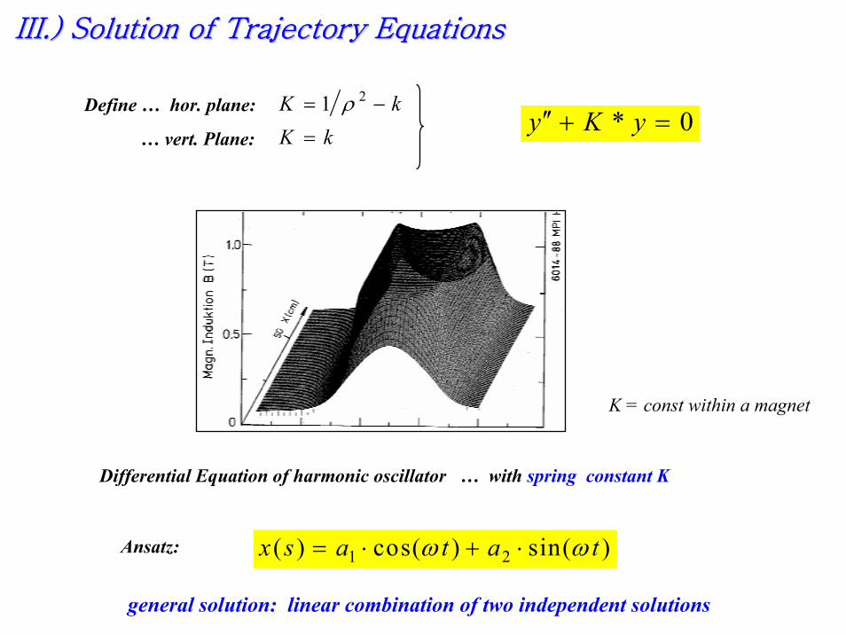
K = const within a magnet

Differential Equation of harmonic oscillator … with spring constant K

1 2( ) cos( ) sin( )= ⋅ + ⋅x s a t a tω ωAnsatz:

general solution: linear combination of two independent solutions

III.) Solution of III.) Solution of TrajectoryTrajectory EquationsEquations

Define … hor. plane:

… vert. Plane:

21= −K kρ* 0′′ + =y K y

=K k

Hor. Focusing Quadrupole K > 0:

0 01( ) cos( ) sin( )′= ⋅ + ⋅x s x K s x K sK

0 0( ) sin( ) cos( )′ ′= − ⋅ ⋅ + ⋅x s x K K s x K s

0

0

(0)(0)

=′ ′=

x xx x starting conditions

For convenience expressed in matrix formalism:

0

⎛ ⎞ ⎛ ⎞= ⋅⎜ ⎟ ⎜ ⎟′ ′⎝ ⎠ ⎝ ⎠

focs

x xM

x x

0

1cos( ) sin(

sin( ) cos( )

⎛ ⎞⎜ ⎟

= ⎜ ⎟⎜ ⎟⎜ ⎟−⎝ ⎠

foc

K s K sKM

K K s K s

1cosh sinh

sinh cosh

⎛ ⎞⎜ ⎟

= ⎜ ⎟⎜ ⎟⎜ ⎟⎝ ⎠

defoc

K l K lKM

K K l K l

hor. defocusing quadrupole: K < 0

drift space: K = 0

10 1

⎛ ⎞= ⎜ ⎟⎝ ⎠

driftl

M

! with the assumptions made, the motion in the horizontal and vertical planes areindependent „ ... the particle motion in x & z is uncoupled“

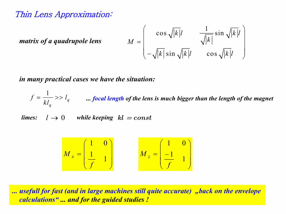
ThinThin LensLens Approximation:Approximation:

1cos sin

sin cos

⎛ ⎞⎜ ⎟

= ⎜ ⎟⎜ ⎟⎜ ⎟−⎝ ⎠

k l k lkM

k k l k l

matrix of a quadrupole lens

in many practical cases we have the situation:

1= >> q

qf l

kl ... focal length of the lens is much bigger than the length of the magnet

0→l kl const=limes: while keeping

1 01 1

⎛ ⎞⎜ ⎟= ⎜ ⎟⎜ ⎟⎝ ⎠

xMf

1 01 1

⎛ ⎞⎜ ⎟= −⎜ ⎟⎜ ⎟⎝ ⎠

zMf

... usefull for fast (and in large machines still quite accurate) „back on the envelopecalculations“ ... and for the guided studies !

focusing lens

dipole magnet

defocusing lens

Transformation through a system of lattice elements

combine the single element solutions by multiplication of the matrices

*.....* * * *= etotal QF D QD B nd DM M M M M M

x(s)

0

typical valuesin a strongfoc. machine:x ≈ mm, x´ ≤ mrad s

court. K. Wille11

122 ´

*´´´

*),(´ sss x

xSCSC

xx

ssMxx

⎟⎟⎠

⎞⎜⎜⎝

⎛⎟⎟⎠

⎞⎜⎜⎝

⎛=⎟⎟

⎠

⎞⎜⎜⎝

⎛=⎟⎟

⎠

⎞⎜⎜⎝

⎛

„C“ and „S“ = sin- and cos- like trajectories of the lattice structure, in other words thetwo independent solutions of the homogeneous equation of motion

Tune: number of oscillations per turn

31.29232.297

Relevant for beam stability:non integer part

0.292*47.3 13.81kHz kHz=

IV.) Orbit & Tune:IV.) Orbit & Tune:

HERA revolution frequency: 47.3 kHz

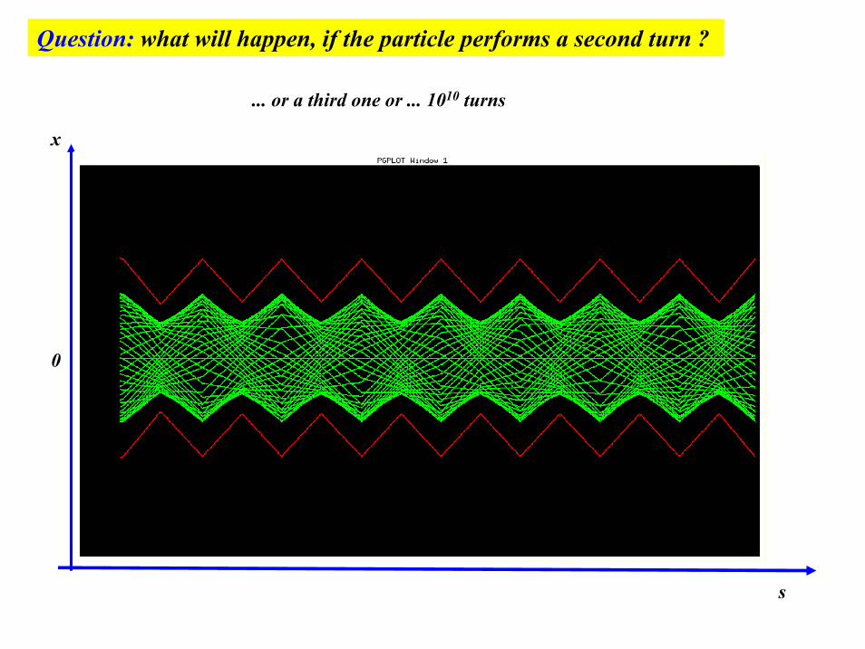
Question: what will happen, if the particle performs a second turn ?

x

... or a third one or ... 1010 turns

0

s

19th century:

Ludwig van Beethoven: „Mondschein Sonate“

Sonate Nr. 14 in cis-Moll (op. 27/II, 1801)

Astronomer Hill:differential equation for motions with periodic focusing properties„Hill‘s equation“

Example: particle motion withperiodic coefficient

equation of motion: ( ) ( ) ( ) 0′′ − =x s k s x s

restoring force ≠ const, we expect a kind of quasi harmonick(s) = depending on the position s oscillation: amplitude & phase will dependk(s+L) = k(s), periodic function on the position s in the ring.

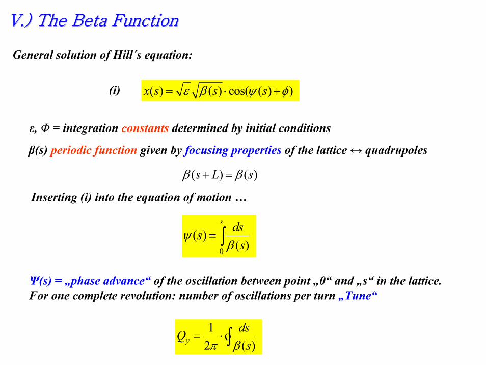
V.) V.) TheThe Beta Beta FunctionFunction

General solution of Hill´s equation:

( ) ( ) cos( ( ) )= ⋅ +x s s sε β ψ φ

β(s) periodic function given by focusing properties of the lattice ↔ quadrupoles

ε, Φ = integration constants determined by initial conditions

Inserting (i) into the equation of motion …

0

( )( )

= ∫s dss

sψ

β

Ψ(s) = „phase advance“ of the oscillation between point „0“ and „s“ in the lattice.For one complete revolution: number of oscillations per turn „Tune“

12 ( )y

dsQsπ β

= ⋅ ∫o

( ) ( )s L sβ β+ =

(i)

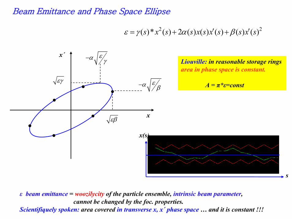
VI.) VI.) BeamBeam EmittanceEmittance and Phase and Phase SpaceSpace EllipseEllipse

(1) ( ) * ( ) *cos( ( ) )= +x s s sε β ψ φ

{ }(2) ( ) * ( )*cos( ( ) ) sin( ( ) )( )

′ = − + + +x s s s ssε α ψ φ ψ φ

β

( )cos( ( ) )* ( )

+ =x ss

sψ φ

ε β

general solution ofHill equation

from (1) we get

Insert into (2) and solve for ε

2 2( )* ( ) 2 ( ) ( ) ( ) ( ) ( )′ ′= + +s x s s x s x s s x sε γ α β

* ε is a constant of the motion … it is independent of „s“* parametric representation of an ellipse in the x x‘ space* shape and orientation of ellipse are given by α, β, γ

2

1( ) ( )2

1 ( )( )( )

− ′=

+=

s s

sss

α β

αγβ

2 2( )* ( ) 2 ( ) ( ) ( ) ( ) ( )′ ′= + +s x s s x s x s s x sε γ α β

BeamBeam EmittanceEmittance and Phase and Phase SpaceSpace EllipseEllipse

x´

xεβ

εα β−εγ

εα γ−

●

●

●

●

●

●x(s)

s

Liouville: in reasonable storage rings area in phase space is constant.

A = π*ε=const

ε beam emittance = woozilycity of the particle ensemble, intrinsic beam parameter, cannot be changed by the foc. properties.

Scientifiquely spoken: area covered in transverse x, x´ phase space … and it is constant !!!

βεσ *=

Ensemble of many (...all) possible particle trajectories

( ) * ( ) *cos( ( ) )= +x s s sε β ψ φmax. amplitude of all particle trajectories

( ) * ( )=x s sε β

Beam Dimension: determined by two parameters

Example: transverse beam profilemeasured using a wirescanner

HERA beam size

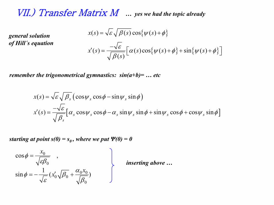
VII.) Transfer Matrix MVII.) Transfer Matrix M … yes we had the topic already

{ }( ) ( ) cos ( )= +x s s sε β ψ φ

{ } { }( ) ( ) cos ( ) sin ( )( )

−′ ⎡ ⎤= + + +⎣ ⎦x s s s ssε α ψ φ ψ φ

β

general solutionof Hill´s equation

remember the trigonometrical gymnastics: sin(a+b)= … etc

( )( ) cos cos sin sin= −s s sx s ε β ψ φ ψ φ

[ ]( ) cos cos sin sin sin cos cos sin−′ = − + +s s s s s ss

x s ε α ψ φ α ψ φ ψ φ ψ φβ

starting at point s(0) = s0 , where we put Ψ(0) = 0

0

0

cos ,=xφεβ

0 00 0

0

1sin ( )′= − +xx αφ β

ε β

inserting above …

{ } { }0 0 0 00

( ) cos sin sin ′= + +ss s s sx s x xβ ψ α ψ β β ψ

β

( ){ } { }00 0 0 0

0

1( ) cos (1 )sin cos sin′ ′= − − + + −s s s s s s sss

x s x xβα α ψ α α ψ ψ α ψββ β

which can be expressed ... for convenience ... in matrix form0

⎛ ⎞ ⎛ ⎞=⎜ ⎟ ⎜ ⎟′ ′⎝ ⎠ ⎝ ⎠s

x xM

x x

( )

( )

0 00

0 0 0

0

cos sin sin

( ) cos (1 )sin cos sin

⎛ ⎞+⎜ ⎟

⎜ ⎟= ⎜ ⎟− − +⎜ ⎟−⎜ ⎟⎝ ⎠

ss s s s

s s s ss s s

s

M

s

β ψ α ψ β β ψβ

α α ψ α α ψ β ψ α ψββ β

* we can calculate the single particle trajectories between two locations in the ring, if we know the α β γ at these positions.

* and nothing but the α β γ at these positions.

* … !

Stability Criterion:

Question: what will happen, if we do not make toomany mistakes and your particle performsone complete turn ?

Matrix for 1 turn:

cos sin sinsin cos sin+⎛ ⎞

=⎜ ⎟− −⎝ ⎠turn s turn s turn

s turn turn s turnM

ψ α ψ β ψγ ψ ψ α ψ

1 0cos sin

0 1α β

ψ ψγ α

⎛ ⎞ ⎛ ⎞= ⋅ +⎜ ⎟ ⎜ ⎟− −⎝ ⎠ ⎝ ⎠

1 JMatrix for N turns:

( )1 cos sin 1 cos sin= ⋅ + ⋅ = ⋅ + ⋅NNM J N J Nψ ψ ψ ψ

The motion for N turns remains bounded, if the elements of MN remain bounded

real=ψ 1cos <↔ ψ 2)( <↔ MTrace

VIII.) Transformation of VIII.) Transformation of αα, , ββ, , γγ

consider two positions in the storage ring: s0 , s0

⎛ ⎞ ⎛ ⎞= ⋅⎜ ⎟ ⎜ ⎟′ ′⎝ ⎠ ⎝ ⎠s s

x xM

x xsince ε = const:

2 2

2 20 0 0 0 0 0 0

2

2

x xx x

x x x x

ε β α γ

ε β α γ

′ ′= + +

′ ′= + +

express x0 , x´0 as a function of x, x´.... remember W = CS´-SC´ = 1

0

0

′ ′= −′ ′ ′= − +

x S x Sxx C x Cx

inserting into ε 2 22′ ′= + +x xx xε β α γ

2 20 0 0( ) 2 ( )( ) ( )′ ′ ′ ′ ′ ′ ′ ′= − + − − + −Cx C x S x Sx Cx C x S x Sxε β α γ

sort via x, x´and compare the coefficients to get ....

●ρ

sθ

z

●

s0

→⎟⎟⎠

⎞⎜⎜⎝

⎛=

´´ SCSC

M

sxx

Mxx

⎟⎟⎠

⎞⎜⎜⎝

⎛=⎟⎟

⎠

⎞⎜⎜⎝

⎛ −

´*

´1

0

⎟⎟⎠

⎞⎜⎜⎝

⎛−

−=−

CCSS

M´

´1

2 20 0 0( ) 2s C SC Sβ β α γ= − +

0 0 0( ) ( )′ ′ ′ ′= − + + −s CC SC S C SSα β α γ2 2

0 0 0( ) 2′ ′ ′ ′= − +s C S C Sγ β α γ

in matrix notation:

2 20

02 2

0

2

2

⎛ ⎞− ⎛ ⎞⎛ ⎞⎜ ⎟ ⎜ ⎟⎜ ⎟ ′ ′ ′ ′= − + − ⋅⎜ ⎟ ⎜ ⎟⎜ ⎟

⎜ ⎟ ⎜ ⎟⎜ ⎟′ ′ ′ ′−⎝ ⎠ ⎝ ⎠⎝ ⎠s

C SC SCC SC CS SS

C S C S

ββα αγ γ

!

1.) this expression is important

2.) given the twiss parameters α, β, γ at any point in the lattice we can transform them and calculate their values at any other point in the ring.

3.) the transfer matrix is given by the focusing properties of the lattice elements, the elements of M are just those that we used to calculate single particle trajectories.

4.) go back to point 1.)

IX.) IX.) RésuméRésumé:: beam rigidity: ⋅ = pB qρ

bending strength of a dipole: 1 00.2998 ( )1( / )

− ⋅⎡ ⎤ =⎣ ⎦B Tm

p GeV cρ

focusing strength of a quadrupole: 2 0.2998( / )

− ⋅⎡ ⎤ =⎣ ⎦gk m

p GeV c

2 02

20.2998( / )

−⎡ ⎤ =⎣ ⎦r

nIk mp GeV c a

μ

focal length of a quadrupole:1

=⋅ q

fk l

equation of motion:1 Δ′′ + =

px Kxpρ

matrix of a foc. quadrupole: 2 1= ⋅s sx M x

1cos sin,

sin cos

⎛ ⎞⎜ ⎟

= ⎜ ⎟⎜ ⎟⎜ ⎟−⎝ ⎠

K l K lKM

K K l K l

1 01 1

⎛ ⎞⎜ ⎟= ⎜ ⎟⎜ ⎟⎝ ⎠

Mf

1.) Asterix der Gallier, Uderzo & Goszini, Verlag Egmont EHAPA / Ed. Albert-René

2.) Edmund Wilson: Introd. to Particle Accelerators Oxford Press, 2001

3.) Klaus Wille: Physics of Particle Accelerators and Synchrotron Radiation Facilicties, Teubner, Stuttgart 1992

4.) Peter Schmüser: Basic Course on Accelerator Optics, CERN Acc.School: 5th general acc. phys. course CERN 94-01

5.) Bernhard Holzer: Lattice Design, CERN Acc. School: Interm.Acc.phys course, http://cas.web.cern.ch/cas/ZEUTHEN/lectures-zeuthen.htm

6.) Herni Bruck: Accelerateurs Circulaires des Particules, presse Universitaires de France, Paris 1966 (english / francais)

7.) M.S. Livingston, J.P. Blewett: Particle Accelerators, Mc Graw-Hill, New York,1962

8.) Frank Hinterberger: Physik der Teilchenbeschleuniger, Springer Verlag 1997

9.) Mathew Sands: The Physics of e+ e- Storage Rings, SLAC report 121, 1970

10.) D. Edwards, M. Syphers : An Introduction to the Physics of ParticleAccelerators, SSC Lab 1990