Introduction_to_synthetic_aperture_sonar.pdf

0

Introduction to Synthetic Aperture Sonar

Roy Edgar HansenNorwegian Defence Research Establishment

Norway

1. Introduction

SONAR is an acronym for SOund Navigation And Ranging. The basic principle of sonar isto use sound to detect or locate objects, typically in the ocean. Sonar technology is similar toother technologies such as: RADAR = RAdio Detection And Ranging; ultrasound, whichtypically is used with higher frequencies in medical applications; and seismic processing,which typically uses lower frequencies in the sediments. There are many good books thatcover the topic of sonar (Burdic, 1984; Lurton, 2010; Urick, 1983). There are also a large numberof books that cover the theory of underwater acoustics more thoroughly (Brekhovskikh &Lysanov, 1982; Medwin & Clay, 1998).The principle of Synthetic aperture sonar (SAS) is to combine successive pings coherentlyalong a known track in order to increase the azimuth (along-track) resolution. A typical datacollection geometry is illustrated in Fig. 1. SAS has the potential to produce high resolutionimages down to centimeter resolution up to hundreds of meters range. This makes SAS asuitable technique for imaging of the seafloor for applications such as search for small objects,imaging of wrecks, underwater archaeology and pipeline inspection.SAS has a very close resemblance with synthetic aperture radar (SAR). While SAS technologyis maturing fast, it is still relatively new compared to SAR. There is a large amount of SARliterature (Carrara et al., 1995; Cumming & Wong, 2005; Curlander & McDonough, 1991;Franceschetti & Lanari, 1999; Jakowatz et al., 1996; Massonnet & Souyris, 2008).This chapter gives an updated introduction to SAS. The intended reader is familiar withsonar but not SAS. The only difference between traditional sonar and synthetic aperture is

Fig. 1. Data acquisition geometry for synthetic aperture sonar.

1

www.intechopen.com

2 Will-be-set-by-IN-TECH

Fig. 2. Basic imaging geometry.

the construction of the aperture (or array). We start by giving a review of sonar imaging anddescribe the backprojection method. Then, we derive the angular resolution. We describe themulti-element receiver concept and calculate the area coverage rate for SAS. We explain thefrequency dependence in SAS, and discuss some of the choices and trade-offs in SAS design.We list some of the specific challenges in SAS, and suggest possible solutions. We give anoverview of the signal processing involved in a SAS processor, and we discuss properties ofSAS images. Finally, we show numerous examples of SAS images from a particular system,the HISAS 1030 interferometric SAS.

2. Sonar Imaging

Assume a transmitter that insonifies a scene with acoustic reflecting material represented bya reflectivity function γ(x, y). A part of the scattered acoustic field is recorded by one or morereceiver hydrophones. This is illustrated in Fig. 2. Sonar imaging is the inverse problem, namelyto estimate the reflectivity function from the received data from one or more transmittedpulses.Sonar imaging can be separated into range processing of the data and angular processing(beamforming) of the data. Beamforming is defined as the method or processing algorithm thatfocuses the signal from several receivers in a particular direction. Beamforming can be appliedto all types of multi-receiver sonars: active, passive, towed array, bistatic, multistatic, andsynthetic aperture. Sonar beamforming is well covered in (Burdic, 1984; Johnson & Dudgeon,1993; Nielsen, 1991).Range processing is signal processing applied to each time series individually. The processingis a function of transmit waveform. There are several types of signals that are used as transmitwaveforms. Classical sonar often uses gated continuous-wave (CW) pulses, sometimesreferred to as pings. Modern sonar, and virtually all SAS systems, use phase coded transmitsignals where the signal bandwidth is determined by the phase coding (or frequency spread ofthe signal modulation). The reason to use phase coded waveforms is to increase the transmitsignal energy while maintaining large signal bandwidth. The range processing done on phasecoded signals are referred to as pulse compression or matched filtering. This is covered in anumber of excellent books such as (Franceschetti & Lanari, 1999; Levanon, 1988).

2.1 Imaging by backprojection

The simplest and most intuitive type of beamforming is time-domain beamforming bybackprojection. This is done by back propagating the received signal via each pixel in the sceneto be imaged and into the transmitter. This is illustrated in Fig. 3. Backprojection is alsoknown as Delay-And-Sum (DAS) (Johnson & Dudgeon, 1993, pages 117-119). Functionally,

4 Sonar Systems

www.intechopen.com

Introduction to Synthetic Aperture Sonar 3

Fig. 3. Backprojection geometry.

backprojection is also closely related to Kirchhoff migration in seismic processing (Claerbout,1995). Formally, backprojection is straightforward and can be done as follows. First the signalsin each receiver are filtered and pulse compressed. Then the signal from each receiver isdelayed to the pixel of interest

tn(x, y) = (rt + rn)/c. (1)

where rt is the distance from the transmitter to the pixel, rn is the distance from the pixel toreceiver n, and c is the sound velocity. Then the recorded, pulse compressed signals sn aresummed coherently over all receivers to produce an estimate of the reflectivity function

γ̂(x, y) =1

N

N

∑n=1

Ansn(tn(x, y)). (2)

The amplitude An is generally a function of geometry and frequency An = An(rt, rr, ω).In addition, the direction dependent sensitivity of the receivers can be taken into account.This amplitude factor can also be used to control the sidelobe suppression vs the angularresolution (Van Trees, 2002). For sampled time series sn(tn(x, y)) may have to be interpolatedto obtain accurate values in the image. A simple algorithmic description of the backprojectionalgorithm is shown in Listing 1. We immediately realise why this method is calledDelay-And-Sum. The signals are delayed to the correct pixel, and then summed.

2.2 Angular resolution

The angular resolution can be defined as the minimum angle for which two reflectors can beseparated in the sonar image. A very simple and intuitive way to derive this is as follows.Assume a phased array receiver of length L consisting of a number of elements as illustratedin Fig. 4. The angular resolution for this receiver is the angle difference for which the echo fromtwo reflectors gives destructive interference in the receivers. Consider a reflector at broadsideand a reflector at an angle β/2. As the maximum range difference will always be on the endsof the array, we only consider the center element and the end element displaced L/2 apart.The distance difference between these two reflectors is

δR = R0 − R1. (3)

5Introduction to Synthetic Aperture Sonar

www.intechopen.com


f o r a l l d i r e c t i o n sf o r a l l ranges

f o r a l l r e c e i v e r sC a l c u l a t e the time delayI n t e r p o l a t e the rece ived time s e r i e sApply appropriate amplitude f a c t o r

endsum over r e c e i v e r s and s t o r e in gamma( x , y )

endend

Listing 1. Backprojection Pseudo-code

For range differences larger than δR = λ/4 destructive interference will start to occur. Thedifference in range is

δR = R0 − R1 = L/2 sin(β/2). (4)

We define β as the angular resolution and solve for when destructive interference will start

δR = L/2 sin(β/2) = λ/4. (5)

For small angles, we can approximate the sin-function

L/2β/2 = λ/4 ⇒ β =λ

L. (6)

Hence, the angular resolution (in radians) equals the inverse length of the array measured inwavelengths. A longer array or a higher frequency (shorter wavelength) gives better angularresolution. More details and a more accurate derivation of angular resolution can be found in(Van Trees, 2002).

2.3 Imaging techniques for phased arrays

Fig. 5 shows the basic imaging geometry for an array of receivers (a phased array). The fieldof view is defined by the beamwidth of each of the receivers and their look direction. The

Fig. 4. Geometrical derivation of angular resolution.

6 Sonar Systems

www.intechopen.com


Fig. 5. Field of view and resolution in imaging sonar.

angular resolution is given by the array length and the wavelength. If the individual elementsare more than λ/2 apart, the directivity of each element must be small enough to mitigate aliaslobes (see section 3.1). For an active system, the range resolution is defined by the bandwidthof the system. The maximum range is determined by the pulse repetition interval and/or thesensitivity of the receiver elements. For a linear array it can be fruitful and efficient for theimaging to define a polar coordinate system fixed to the sonar.In underwater applications, beamforming can be used to produce different types of products.For high frequency sonar imaging, this can be categorized into three different types, asillustrated in Fig. 6:

Sectorscan sonar produces a two-dimensional image for each pulse. These images areusually shown on a display pulse by pulse. Sectorscanning sonar is often used ashull mounted sonars for forward looking imaging or wide swath imaging. In fisheriesacoustics, some cylindrical arrays actually produce full 360 degrees view.

Sidescan sonar is a particular type of sonar that uses the platform motion to cover differentparts of the seafloor. A sidescan sonar produces one or a few beams around broadside,and an image of the seafloor is produced by moving the sonar and using repeated pulses.This is a very popular technology, it has fairly low hardware complexity and can thereforebe more affordable. There are several books covering sidescan sonar very thoroughly(Blondel, 2009; Fish & Carr, 2001).

Synthetic aperture sonar uses multiple pulses to create a large synthetic array (or aperture).From this, an image of the seafloor is produced such that the information from multiplepulses goes into each pixel on the seafloor. It is, from a certain point of view, thecombination of sidescan sonar and sectorscan sonar.

3. SAS sampling and coverage rate

In all types of array signal processing, the sampling of the array, or the spacing of the elementsand their directivity, is critical. If the array is too sparsely sampled, grating or alias lobes will


www.intechopen.com


Fig. 6. Phased array imaging concepts for sonar.

occur, and the image quality will be reduced. In this section we describe the sampling criterionand show how this affects SAS design.

3.1 Undersampling of arrays

Consider a simple array with two elements displaced D apart, as illustrated in Fig. 7. Assumean inbound plane wave at broadside θ = 0 with wavelength λ from a reflector in the far field.Any plane wave coming in the direction

sin θn = ±nλ

2D(7)

where n is an integer, will be perfectly in phase with the plane wave at broadside. Note that thefactor two, i.e. λ/2, comes from assuming two-way propagation (transmission and reception).This ambiguity will cause grating lobes or alias lobes in the beampattern (Manolakis et al.,2000; Van Trees, 2002). To avoid grating lobes, the beamwidth of each individual elementmust be smaller than the distance to the first grating lobe. Assuming that each element is ofsize d with a beamwidth of β ≈ λ/d, we get the sampling criterion

D ≤ d/2. (8)

Hence, for a well sampled array, the effective distance between each element must be half thesize of each element. This is fulfilled for a densely populated array without gaps betweenelements (see below).Grating lobes are such that the problem they cause cannot be fixed in signal processingafterwards. For linear uniform arrays (ULAs), there is a deterministic and simple one-to-one

Fig. 7. Along track sampling and grating (alias) lobes.

8 Sonar Systems

www.intechopen.com


Fig. 8. Multi-element receiver array and the Phase Center Approximation.

relation between the sampling of the array and the angular position of the grating lobes.Grating lobes are frequency dependent. For large bandwidth systems, the grating lobes willbe less defined due to the fact that their positions change with frequency.

3.2 Multi-element receiver arrays in SAS

In SAS, the transmitter-receiver pair is moved along-track and pulsed repeatedly to form along synthetic antenna. The sampling criterion (8) imposes a maximum allowed displacementbetween pings, which again, transforms into a maximum range for a given speed. Themaximum range Rmax is given by

2Rmax/c = Tpri = D/v ⇒ Rmax =cD

2v(9)

where v is the platform speed and Tpri is the pulse repetition interval. This relation imposesa very strong limitation to SAS. Consider a platform speed of v = 2 m/s. For a displacementof D = 5 cm, the maximum range then becomes Rmax = 18.75 m for a sound velocity ofc = 1500 m/s. This is an unacceptable small range for most applications. To overcomethis, a receiver array of multiple elements can be used (Bruce, 1992; Cutrona, 1975). Themulti-element receiver array is used in almost all existing SAS systems today.A simple description of how a single transmitter multiple receiver system can be used toform a synthetic aperture is as follows. Consider a single transmitter Tx and N receiversof size d in a linear array Rx, as illustration shown in Fig. 8. In stead of treating this as abistatic system with one transmitter and many receivers, we assume a virtual array where eachelement is placed at the middle position between each transmitter-receiver pair (indicatedin light green). In this array, each element is a transmitter-receiver (monostatic). This is thePhase Center Approximation (PCA) (Bellettini & Pinto, 2002). The virtual array (or PCA array)is half the length of the receiver array, with element size d/2, and each of the elements inthe virtual array can be placed directly in a synthetic array (similar to SAR). The maximumdisplacement between two pulses becomes the length of the PCA array D = Nd/2 = L/2,and the maximum range becomes

Rmax =cL

4v(10)

where L is the length of the receiver array. The maximum range can then be increased byincreasing the length of the receiver array. Fig. 9 shows the maximum range as function ofvehicle speed for three different receiver array lengths. Note that the area coverage rate (speedtimes range) is a constant proportional to the array length.In airborne SAR, aperture undersampling is not a problem, since the phase velocity forelectromagnetic waves in air is relatively high compared to the platform speed. In large


www.intechopen.com


Fig. 9. Maximum range for given platform speed for three different receiver array lengths.

swath high resolution space-borne SAR, there is a limitation related to the sampling criterion.Advanced SAR systems have 2D phased arrays and use electronic steering of the transmitterand receiver arrays for different SAR modes. ScanSAR (Franceschetti & Lanari, 1999) andTerrain Observation by Progressive Scans (TOPS) (Gebert et al., 2010) are used to increase thearea coverage rate while lowering the resolution. Spotlight mode (Jakowatz et al., 1996) isused to increase the resolution while lowering the area coverage rate.

4. Design of Synthetic Aperture Sonar

SAS is different from traditional sonar in several ways. In this section we describe some of thesignificant differences that affect the performance and application areas of SAS.

4.1 Resolution

While traditional imaging sonar has constant angular resolution, and thereby rangedependent along-track resolution, SAS produces range independent along-track resolution.This is done by increasing the length of the synthetic array as function of range. Consider theleft illustration of Fig. 10. The maximum length of the synthetic aperture is given by the fieldof view of each transmitter/receiver element. At range R1, the length of the synthetic aperturebecomes

L1 ≈ βR1 (11)

where β = λ/d is the field of view. The along-track resolution is given by the syntheticantenna

δx ≈ R1λ

2L1(12)

where the factor 2 comes from the fact that both the transmitter and receiver is moved alongthe synthetic aperture (creating a focused receiver and transmitter). Inserting for L1 and β weget a resolution of

δx ≈ R1λ

2L1= R1

λ

2βR1= R1

λ

2λ/dR1=

d

2. (13)

10 Sonar Systems

www.intechopen.com


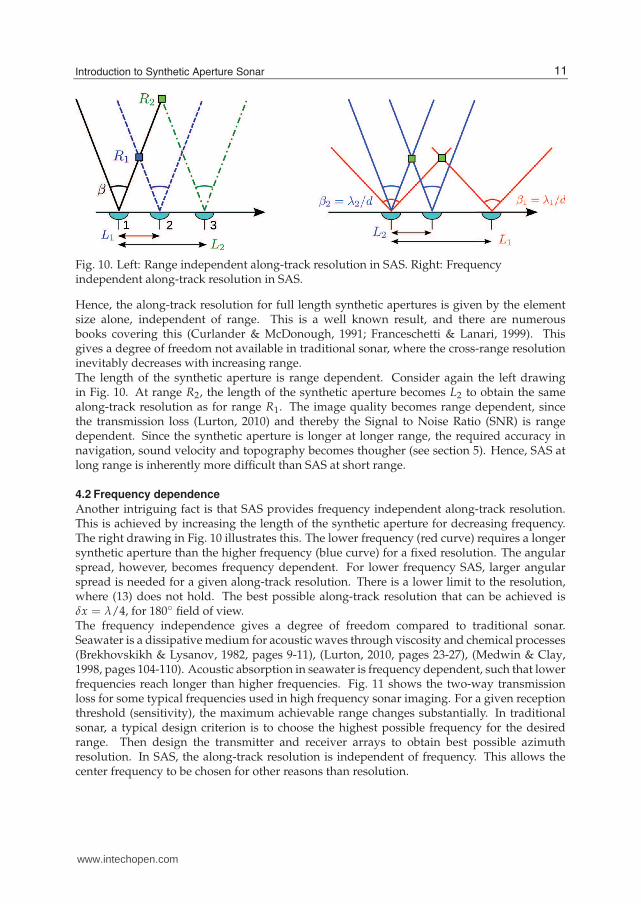
Fig. 10. Left: Range independent along-track resolution in SAS. Right: Frequencyindependent along-track resolution in SAS.

Hence, the along-track resolution for full length synthetic apertures is given by the elementsize alone, independent of range. This is a well known result, and there are numerousbooks covering this (Curlander & McDonough, 1991; Franceschetti & Lanari, 1999). Thisgives a degree of freedom not available in traditional sonar, where the cross-range resolutioninevitably decreases with increasing range.The length of the synthetic aperture is range dependent. Consider again the left drawingin Fig. 10. At range R2, the length of the synthetic aperture becomes L2 to obtain the samealong-track resolution as for range R1. The image quality becomes range dependent, sincethe transmission loss (Lurton, 2010) and thereby the Signal to Noise Ratio (SNR) is rangedependent. Since the synthetic aperture is longer at longer range, the required accuracy innavigation, sound velocity and topography becomes thougher (see section 5). Hence, SAS atlong range is inherently more difficult than SAS at short range.

4.2 Frequency dependence

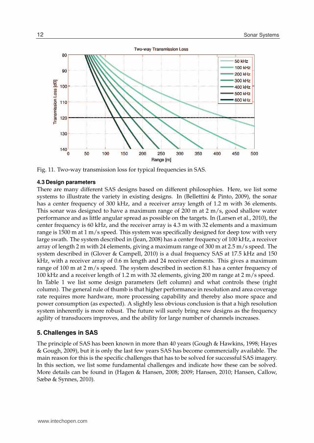
Another intriguing fact is that SAS provides frequency independent along-track resolution.This is achieved by increasing the length of the synthetic aperture for decreasing frequency.The right drawing in Fig. 10 illustrates this. The lower frequency (red curve) requires a longersynthetic aperture than the higher frequency (blue curve) for a fixed resolution. The angularspread, however, becomes frequency dependent. For lower frequency SAS, larger angularspread is needed for a given along-track resolution. There is a lower limit to the resolution,where (13) does not hold. The best possible along-track resolution that can be achieved isδx = λ/4, for 180◦ field of view.The frequency independence gives a degree of freedom compared to traditional sonar.Seawater is a dissipative medium for acoustic waves through viscosity and chemical processes(Brekhovskikh & Lysanov, 1982, pages 9-11), (Lurton, 2010, pages 23-27), (Medwin & Clay,1998, pages 104-110). Acoustic absorption in seawater is frequency dependent, such that lowerfrequencies reach longer than higher frequencies. Fig. 11 shows the two-way transmissionloss for some typical frequencies used in high frequency sonar imaging. For a given receptionthreshold (sensitivity), the maximum achievable range changes substantially. In traditionalsonar, a typical design criterion is to choose the highest possible frequency for the desiredrange. Then design the transmitter and receiver arrays to obtain best possible azimuthresolution. In SAS, the along-track resolution is independent of frequency. This allows thecenter frequency to be chosen for other reasons than resolution.


www.intechopen.com


Fig. 11. Two-way transmission loss for typical frequencies in SAS.

4.3 Design parameters

There are many different SAS designs based on different philosophies. Here, we list somesystems to illustrate the variety in existing designs. In (Bellettini & Pinto, 2009), the sonarhas a center frequency of 300 kHz, and a receiver array length of 1.2 m with 36 elements.This sonar was designed to have a maximum range of 200 m at 2 m/s, good shallow waterperformance and as little angular spread as possible on the targets. In (Larsen et al., 2010), thecenter frequency is 60 kHz, and the receiver array is 4.3 m with 32 elements and a maximumrange is 1500 m at 1 m/s speed. This system was specifically designed for deep tow with verylarge swath. The system described in (Jean, 2008) has a center frequency of 100 kHz, a receiverarray of length 2 m with 24 elements, giving a maximum range of 300 m at 2.5 m/s speed. Thesystem described in (Glover & Campell, 2010) is a dual frequency SAS at 17.5 kHz and 150kHz, with a receiver array of 0.6 m length and 24 receiver elements. This gives a maximumrange of 100 m at 2 m/s speed. The system described in section 8.1 has a center frequency of100 kHz and a receiver length of 1.2 m with 32 elements, giving 200 m range at 2 m/s speed.In Table 1 we list some design parameters (left column) and what controls these (rightcolumn). The general rule of thumb is that higher performance in resolution and area coveragerate requires more hardware, more processing capability and thereby also more space andpower consumption (as expected). A slightly less obvious conclusion is that a high resolutionsystem inherently is more robust. The future will surely bring new designs as the frequencyagility of transducers improves, and the ability for large number of channels increases.

5. Challenges in SAS

The principle of SAS has been known in more than 40 years (Gough & Hawkins, 1998; Hayes& Gough, 2009), but it is only the last few years SAS has become commercially available. Themain reason for this is the specific challenges that has to be solved for successful SAS imagery.In this section, we list some fundamental challenges and indicate how these can be solved.More details can be found in (Hagen & Hansen, 2008; 2009; Hansen, 2010; Hansen, Callow,Sæbø & Synnes, 2010).

12 Sonar Systems

www.intechopen.com


Design Parameter Relation

Range resolution System Bandwidth

Along-track resolution Element size

Area coverage rate Receiver array length

Maximum range Frequency, receiver array length and speed

Signal to Noise Ratio Frequency, geometry and maximum range

Robustness Relative bandwidth and redundancy

Complexity Beamwidth, number of elements and relative bandwidth

Throughput Bandwidth times number of receiver elements

Table 1. Design parameters and their relation in SAS.

5.1 Navigation

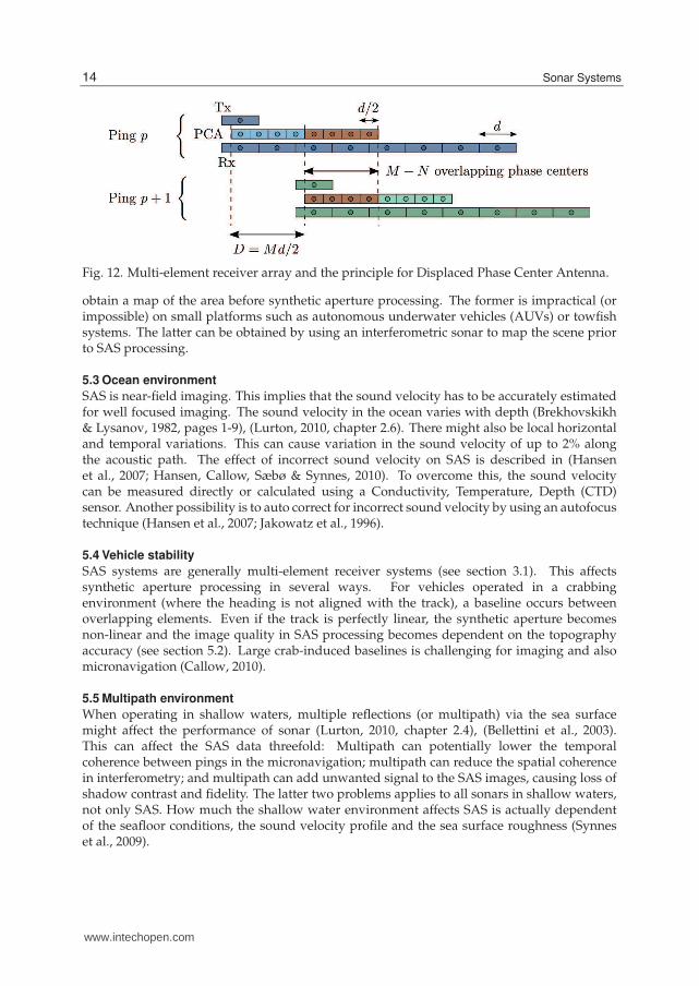
The sonar has to be positioned with accuracy better than a fraction of a wavelength along thesynthetic aperture. This is the same requirement as for any other array sensor, but inherentlymore difficult to obtain since a synthetic antenna is formed by a moving platform. A sharpimage depends on accurate positioning of the elements in the array. How much error istolerated is dependent on the scale of the error and the required image quality (Carrara et al.,1995). Navigation of underwater platforms is more difficult than navigation of airborne andterrestrial platforms because GPS is not available. This challenge is the most important, andthe first that has to be overcome for successful SAS imagery.One solution is to use the sonar data itself for navigation (referred to as micronavigation).Compare the illustration in Fig. 12 with Fig. 8. By moving the SAS system a distanceD = Md/2 such that M < N, there will be redundancy (or overlap) in the synthetic aperture.The overlap in the phase center antenna (PCA) is indicated in orange. Estimating whichchannels overlap can be used to estimate the displacement along-track and cross-track. Thiscan be done by cross correlating the data recorded by elements from ping p with data recordedby other elements from ping p + 1. The method is named displaced phase center antenna(DPCA) or redundant phase center (RPC). DPCA was first used in Moving Target Indicator(MTI) radars in the 1950s (Dickey Jr et al., 1991). In SAS, early descriptions of DPCA can befound in (Pinto et al., 1997; Sheriff, 1992). A very good overview of the method is given in(Pinto, 2002), and a detailed study of the performance is given in (Bellettini & Pinto, 2002). In(Hansen et al., 2003) different strategies to combine DPCA with traditional inertial navigationis described.Micronavigation using DPCA causes a trade-off between navigation performance andefficiency (area coverage rate). This is due to the fact that the displacement between pingshas to be less than the maximum displacement L/2. More overlap gives better navigation butlower area coverage rate. An exception to this is if several transmitters, specific bandwidth,and a specific pulse regime is used (Billon & Fohanno, 2002).

5.2 Topographic errors

When running a vehicle on a non-straight track, a non-straight synthetic aperture is formedand the imaging geometry becomes dependent on the full three-dimensional geometry. Thismeans that the position of the sonar has to be known and the topography (or bathymetry)of the scene to be imaged has to be known (Jakowatz et al., 1996, pages 187-197). Onlythen, successful SAS processing can be done. This is critical for robust SAS, and a significantproblem since the topographic changes in rough terrain may impose severe non-linear tracks(Hansen et al., 2009). There are two solutions to this challenge: either run on a straight line or


www.intechopen.com


Fig. 12. Multi-element receiver array and the principle for Displaced Phase Center Antenna.

obtain a map of the area before synthetic aperture processing. The former is impractical (orimpossible) on small platforms such as autonomous underwater vehicles (AUVs) or towfishsystems. The latter can be obtained by using an interferometric sonar to map the scene priorto SAS processing.

5.3 Ocean environment

SAS is near-field imaging. This implies that the sound velocity has to be accurately estimatedfor well focused imaging. The sound velocity in the ocean varies with depth (Brekhovskikh& Lysanov, 1982, pages 1-9), (Lurton, 2010, chapter 2.6). There might also be local horizontaland temporal variations. This can cause variation in the sound velocity of up to 2% alongthe acoustic path. The effect of incorrect sound velocity on SAS is described in (Hansenet al., 2007; Hansen, Callow, Sæbø & Synnes, 2010). To overcome this, the sound velocitycan be measured directly or calculated using a Conductivity, Temperature, Depth (CTD)sensor. Another possibility is to auto correct for incorrect sound velocity by using an autofocustechnique (Hansen et al., 2007; Jakowatz et al., 1996).

5.4 Vehicle stability

SAS systems are generally multi-element receiver systems (see section 3.1). This affectssynthetic aperture processing in several ways. For vehicles operated in a crabbingenvironment (where the heading is not aligned with the track), a baseline occurs betweenoverlapping elements. Even if the track is perfectly linear, the synthetic aperture becomesnon-linear and the image quality in SAS processing becomes dependent on the topographyaccuracy (see section 5.2). Large crab-induced baselines is challenging for imaging and alsomicronavigation (Callow, 2010).

5.5 Multipath environment

When operating in shallow waters, multiple reflections (or multipath) via the sea surfacemight affect the performance of sonar (Lurton, 2010, chapter 2.4), (Bellettini et al., 2003).This can affect the SAS data threefold: Multipath can potentially lower the temporalcoherence between pings in the micronavigation; multipath can reduce the spatial coherencein interferometry; and multipath can add unwanted signal to the SAS images, causing loss ofshadow contrast and fidelity. The latter two problems applies to all sonars in shallow waters,not only SAS. How much the shallow water environment affects SAS is actually dependentof the seafloor conditions, the sound velocity profile and the sea surface roughness (Synneset al., 2009).

14 Sonar Systems

www.intechopen.com


Fig. 13. Overview of SAS signal processing flow.

6. Signal processing of SAS data

Signal processing of SAS data can be done in many different ways. Fig. 13 shows the shcematicoverview of a processing flow. Signal processing of SAS data is similar to SAR processing,with a few exceptions. Accurate knowledge of the vehicle navigation (track position andsensor orientation), the ocean environment and in particular the sound velocity, and theseafloor topography must be obtained for successful SAS imagery (see section 5).The first step (blocking) in the processing is to divide the data into portions suitable forsynthetic aperture processing. The blocking selects which pings to put into one syntheticaperture, and decides what to do with the data. If micronavigation is required, thismust take place before imaging. There are two classes of image formation algorithms:time domain imaging and frequency domain imaging. In general, the frequency domainalgorithms are more efficient but require more controlled vehicle behavior (close to straightline tracks). Candidates are the wavenumber algorithm (Soumekh, 1994),(Cumming & Wong,2005, chapter 8), (Carrara et al., 1995, chapter 10) (also referred to as range migration algorithmor Omega-K algorithm), and the chirp scaling algorithm (Cumming & Wong, 2005, chapter 7),(Franceschetti & Lanari, 1999). Alternatively, the image formation can be done in time domain(see section 2.1). An overview of different algorithms used in SAS imaging can be found in(Gough & Hawkins, 1997).The benefit of time domain beamforming is that the imaging gridcan be arbitrary and the data acquisition (the synthetic aperture) can be severely distorted.This gives an added flexibility not available in frequency domain imaging (Massonnet &Souyris, 2008, chapter 2.4). The disadvantage of time domain imaging is the computationalload. After image formation, blind correction for residual errors (known as autofocus) inthe image can be performed (Jakowatz et al., 1996, chapter 4), (Callow, 2003). It should benoted that most autofocusing techniques are local methods - they have a certain success incorrecting local errors, but do not perform well on a large image with different sources forerrors in different locations in the image. For interferometric systems, the final stage in theSAS processing flow is bathymetry estimation using interferometry (Hanssen, 2001; Sæbø,2010).


www.intechopen.com


7. Properties of SAS images

The goal of sonar imaging is to estimate the acoustic reflectivity in the best possible manner,given the sensor and geometry (see section 2). (Oliver & Quegan, 1998) gives an excellentoverview of the properties of SAR images (highly relevant for SAS), related to the signalprocessing and the scene content. In the following, we list common measures of systemperformance, applicable to any imaging system.

Geometrical resolution or detail resolution. This is the minimum distance between tworeflectors where they can be resolved in the image. The theoretical geometric resolution isgiven by the bandwidth for the range dimension and the element size for the along-trackdimension (see section 4.1). The true geometrical resolution is also dependent on the imagequality. Defocus will reduce the geometrical resolution (Oliver & Quegan, 1998, chapter3.2).

Radiometric resolution or contrast / value resolution, echogenicity or target strengthaccuracy. This is the accuracy of the estimated value in each pixel. All coherent imagingsystems suffers from speckle (Goodman, 2007; Oliver & Quegan, 1998). Speckle israndom variability caused by constructive and destructive interference between individualscatterers in each geometrical resolution cell. Speckle causes a variance in the pixel valueand thereby a reduced radiometric resolution. There are different methods to despeckleimages and to estimate the scattering cross section. The traditional approach in SARhas been to apply multilook processing to reduce speckle (Jakowatz et al., 1996, chapter3.3). There also exist more advanced methods to estimate the scattering cross section(Massonnet & Souyris, 2008, chapter 3.11), (Oliver & Quegan, 1998, chapter 6). Theradiometric resolution strictly depends on a fully calibrated system, where the wholesystem has to be energy preserving. This is non-trivial to obtain, and it implies that allthe terms except the Target Strength in the sonar equation has to be accounted for (Ainslie,2010; Lurton, 2010), (Curlander & McDonough, 1991, chapter 7).

Dynamic range or resolvability of small targets in the presence of large targets. This is afunction of the sidelobe levels or the shape of the point spread function. There is a trade-offbetween geometrical resolution and dynamic range. Large dynamic range requires largesidelobe suppression which causes poorer geometrical resolution (Franceschetti & Lanari,1999, chapter 3.1), (Carrara et al., 1995, chapter 8). In addition to the sidelobes, the aliaslobes (or grating lobes) must also be controlled in order to obtain the desired dynamicrange. This can only be achieved by oversampling the synthetic aperture (Bellettini &Pinto, 2009; Gough & Hawkins, 1997).

Sensitivity or detection ability of low level targets. This is determined by several of the termsin the sonar equation (Lurton, 2010; Urick, 1983), such as system self noise, transmit power,transmission loss (which is a function of acoustic frequency) and processing gain. See(Ainslie, 2010) for a detailed description of the terms in the sonar equation. A system withlarger pulse compression gain will have improved sensitivity.

Temporal resolution or framerate. This is the number of independent images on the sceneper unit time. Since SAS is based on space-time processing (spatial movement uses time togenerate aperture), SAS only has one frame on the scene when using full aperture length.Multi-aspect imaging (Hansen et al., 2008) can be applied to produce multiple aspects fromdifferent apertures and thereby different time intervals. There is a trade-off between looksand along-track resolution (since the aperture becomes shorter).

16 Sonar Systems

www.intechopen.com


Fig. 14. The ability to retrieve relevant information from a SAS image is dependent on anumber of different factors.

The ability to extract the relevant information from a SAS image depends on a number ofdifferent factors, as illustrated in Fig. 14. Observation geometry given by range and elevationangle is important for interpretation of the highlight structure and shadow. Backscatteredtarget signals can contain elements of specular reflections, diffuse scattering, transparency,resonant scattering and multiple scattering, all of which complicate the process of retrievingthe relevant information. Finally, image resolution is critical in resolving or classifying objects,shadow shape and the surrounding scatterers on the seafloor.

8. Applications of SAS

There are many applications where SAS is suitable. Very high resolution acoustic imagingcan be achieved on traditional sonar using very high frequencies, and there are sonar systemstoday using up to 2 MHz frequency. They are, hovewer, very limited in range. When largearea coverage and very high resolution is needed at the same time, SAS is really the onlytechnology that can provide a solution. In this section, we describe a particular SAS system,the HISAS 1030, and show example images from different applications.

8.1 The HISAS 1030 interferometric SAS

HISAS 1030 is a wideband widebeam interferometric SAS developed by Kongsberg Maritimeand FFI (Fossum et al., 2008; Hagen et al., 2008). The sonar contains two along-track receiverarrays of 1.2 m length with 32 elements in each array, and a vertical baseline approximately30 cm which equals 20 wavelengths. The transmitter is a vertical phased array with 16elements, and the transmit beam can be electronically steered and shaped to obtain the bestpossible performance in shallow waters (see Section 5.5). The transmitter can also be used as areceiver, giving 16 individual receiver channels along a vertical array. Fig. 15 shows the sonarmounted on a HUGIN 1000-MR AUV. Typical HISAS 1030 specifications are listed in Table2. The SAS processing is done in a software suite named FOCUS Toolbox (Hansen et al., 2005;2003).Fig. 16 shows an example SAS image made by the HISAS 1030 on the HUGIN 1000 AUV. Theimage shows the wreck of the 1500 dwt oil tanker Holmengraa lying on a slanted seabed at


www.intechopen.com


Fig. 15. The HISAS 1030 interferometric SAS on the HUGIN autonomous underwatervehicle. The picture was taken just before launch during a scientific mission on board theresearch vessel H U Sverdrup II in Norwegian waters in April 2010.

Center frequency 100 kHz

Wavelength 1.5 cm

Bandwidth 30 kHz

Total frequency range 50-120 kHz

Along-track resolution 3 cm

Cross-track resolution 3 cm

Maximum range @ 2 m/s 200 m

Area coverage rate 2 km2/h

Table 2. Typical system specifications for the HISAS 1030 interferometric SAS.

depth 77 m. The distance to the center of the image is about 95 m. The length of the wreck isabout 68 m and width about 9 m.Fig. 17 captures the essence of SAS: Long range and high resolution at the same time. The large(middle) image shows a SAS image where the range is 25 m (left) to 325 m (right), and thedynamic range is 32 dB. The data was collected with HISAS 1030 on HUGIN AUV running at2.3 knots at 40 m altitude, outside Horten, Norway in approximately 200 m water depth. Theupper image shows a section from 200 m range to 250 m range with the wreck of the GermanWWII submarine U735. The lower image shows a section from 260 m range to 290 m rangewith a 1 m3 cube. The length of the synthetic aperture is (see section 4.1)

Lsa ≈ Rηλ

d(14)

18 Sonar Systems

www.intechopen.com


Fig. 16. SAS image of the wreck of the Norwegian tanker Holmengraa that was sunk duringWWII in 1944. Courtesy of Kongsberg Maritime.

where R is the range, λ is the wavelength at center frequency, d is the along-track elementsize in the array. η is a programmable parameter controlling the process beamwidth, that is, thebeamwidth actually processed. In this particular case, η = 2/3, and the length of the syntheticaperture at maximum range becomes Lsa ≈ 90 m = 6000λ. The SAS resolution-gain, definedas the ratio between along-track resolution in real aperture δxra and synthetic aperture δxsa is

Qsa =δxra

δxsa=

Lsa

L/2≈ Rη

2λ

Ld, (15)

where and L is the array length. In Fig. 17, the SAS resolution-gain is Qsa ≈ 150 at maximumrange. This is a considerable resolution improvement, and the equivalent along-trackresolution is very difficult to obtain using real aperture techniques.

8.2 Underwater archaeology

SAS is a candidate technology in searching for wrecks and other objects of historic interest.Fig. 18 shows a SAS image collected by the Royal Norwegian Navy in a training mission closeto the town of Tromsø in the winter of 2009. The data was collected at 34 m water depth,close to shore. The image shows the wreck of a German WWII Heinkel He 115 seaplane. Theoriginal length of the plane is 17 m and the wingspan was 22 m. Note the small part outsidethe right wing of the seaplane. This is probably one of the floats. The object in the lower leftpart of the image is probably the tail-section of another plane of the same type.


www.intechopen.com


Fig. 17. Middle: SAS image where the range is 25 m (left) to 325 m (right). Courtesy ofKongsberg Maritime.

20 Sonar Systems

www.intechopen.com


Fig. 18. SAS image of a German WWII Heinkel He 115 seaplane lying on the seafloor.Courtesy of the Royal Norwegian Navy. Photograph is from wikipedia.

8.3 Search for small objects

When searching for small objects over very large areas, SAS is an excellent tool. Fig. 19 showsa SAS image from an area with debris. The sonar has traveled along the vertical directionof the image, and the sonar look direction is towards right. The size of the image is 190 m(along-track) and 30 m to 165 m cross-track, and the water depth is around 70 m. The yellowboxes indicates three objects, and the small images below show zoomed images of the objects.These are two drums of approximate size 0.9 m length and 0.6 m diameter, and a cylinder ofapproximate length 2.5 m. The lower row of images shows optical images of the same objects.The optical images were collected with another HUGIN AUV. The altitude was 5 m on thedata collection of the optical images. We see several interesting features in the objects. Thedrum at 73 m has clear indications of partial transparency. The back end of the barrel is clearlyvisible, and there is acoustic pollution in the shadow region. The drum at 112 m has a lessdefined back end and deeper shadow contrast, indicating that this object is less transparent.In the optical images, indeed, we see that the drum at 73 m has severe damage and holes,while the drum at 112 m looks to be more intact. In the optical image of the cylinder, we see asmall cavity in the lower right end. This appears as a highlight in the SAS image.


www.intechopen.com


Fig. 19. Upper: SAS image of an area with small objects. The range is 30 m (left) to 165 m(right), and the along-track (vertical) is 190 m. The small cut-outs shows zoomed images ofthree different objects. The lower row shows optical images of the same targets. Courtesy ofKongsberg Maritime / FFI.

22 Sonar Systems

www.intechopen.com


8.4 Inspection of man made constructions

External inspection of underwater constructions such as pipelines is an important task. Theobjective of these inspections is to detect burial, exposure, free spans and buckling of thepipeline, as well as possible damages due to trawling, anchoring and debris near the pipeline.SAS may be well suited technology for some of these tasks (Hagen et al., 2010), (Hansen,Sæbø, Callow & Hagen, 2010). Fig. 20 shows an example SAS image collected by a HUGINAUV during a demonstration in San Diego, USA, in 2010. The image shows a sewer pipeline,and a rope or wire on the seafloor.

Fig. 20. Upper: SAS image of a pipeline outside San Diego. The range in the upper image is65 m - 145 m. Lower: 20 m times 10 m zoomed area at range 85 m of a rope or wire on theseafloor. Courtesy of Kongsberg Maritime.


www.intechopen.com

(a) SAS image 1 (b) SAS image 2

9. Conclusion

Synthetic aperture sonar (SAS) is an advanced signal processing technique to improveresolution in sonar imagery. The main application is detailed documentation of the seafloor,in areas such as search for small objects, underwater archaeology, detailed seabed mappingand documentation of underwater installations. Successful SAS is dependent on accurateknowledge about the sonar position, the ocean environment and the seabed topography.SAS is substantially more mature now than 10 years ago. To illustrate the maturity ofcommercially available systems, we show a final example of SAS data collected by the HUGINAUV carrying the HISAS 1030. Fig. 21 shows SAS images and interferometric SAS relativebathymetries of a German WWII Focke Wulf 190 A-3 aeroplane that was found by the RoyalNorwegian Navy mine warfare flotilla. The length of the plane is 9 m and the wingspan is10.5 m. The tail was damaged as we see in the SAS images and the bathymetries. The motorfell off during the recovery. These images was produced at sea by the Royal Norwegian Navypersonnel during the search operation. The images was constructed using micronavigationand sidescan bathymetry as a preprocessing step, then backprojection in three dimensionsfor image formation, and finally bathymetry estimation using a maximum likelihood phaseestimator in the interferometric processing.

10. Acknowledgments

The author thanks the very good colleagues Hayden J Callow, Torstein O Sæbø, and StigA V Synnes at the Norwegian Defence Research Establishment. The author also thankKongsberg Maritime, and in particular Per Espen Hagen and Bjørnar Langli, for a longstanding collaboration and providing data for the analysis. Finally the author wish to thankthe Royal Norwegian Navy Mine Warfare Service for the long fruitful collaboration and kindpermission to use data recorded during Navy operations with their HUGIN 1000-MR AUV.

24 Sonar Systems

www.intechopen.com

(c) Bathymetry by SAS interferometry 1 (d) Bathymetry by SAS interferometry 2

Fig. 21. The German WWII Focke Wulf 190 A-3 aircraft. The plane was found by the RoyalNorwegian Navy Mine warfare flotilla at 98 m water depth during an underwaterarchaeology mission. Courtesy of the Royal Norwegian Navy.

(e) Photograph taken during the recovery (f) Photograph taken during the recovery


www.intechopen.com


11. References

Ainslie, M. (2010). Principles of Sonar Performance Modelling, Springer Verlag.Bellettini, A. & Pinto, M. A. (2002). Theoretical accuracy of synthetic aperture sonar

micronavigation using a displaced phase-center antenna, IEEE J. Oceanic Eng.27(4): 780–789.

Bellettini, A. & Pinto, M. A. (2009). Design and Experimental Results of a 300-kHz SyntheticAperture Sonar Optimized for Shallow-Water Operations, IEEE J. Oceanic Eng.34(3): 285–293.

Bellettini, A., Pinto, M. A. & Wang, L. (2003). Effect of multipath on synthetic aperture sonar,Proc. 5th World Congr. Ultrasonics, Paris, France, pp. 531–534.

Billon, D. & Fohanno, F. (2002). Two improved ping-to-ping cross-correlation methods forsynthetic aperture sonar: theory and sea results, OCEANS’02 MTS/IEEE, Vol. 4, IEEE,pp. 2284–2293.

Blondel, P. (2009). The Handbook of Sidescan Sonar, Geophysical Sciences, Springer Praxis Books.Brekhovskikh, L. & Lysanov, Y. (1982). Fundamentals of Ocean Acoustics, Vol. 8 of Springer Series

in Electrophysics, Springer-Verlag, Berlin, Germany.Bruce, M. P. (1992). A processing requirement and resolution capability comparison of

side-scan and synthetic-aperture sonars, IEEE J. Oceanic Eng. 17(1): 106–117.Burdic, W. S. (1984). Underwater acoustic system analysis, Prentice Hall.Callow, H. J. (2003). Signal Processing for Synthetic Aperture Sonar Image Enhancement, PhD

thesis, University of Canterbury, Christchurch, New Zealand.Callow, H. J. (2010). Comparison of SAS processing strategies for crabbing collection

geometries, Proceedings of Oceans 2010 MTS/IEEE, Seattle, US.Carrara, W. G., Goodman, R. S. & Majewski, R. M. (1995). Spotlight Synthetic Aperture Radar:

Signal Processing Algorithms, Artech House.Claerbout, J. (1995). Basic earth imaging, Stanford Exploration Project.

URL: http://sepwww.stanford.edu/Cumming, I. G. & Wong, F. H. (2005). Digital Processing of Synthetic Aperture Radar Data:

Alogirthms and Implementation, Artech House.Curlander, J. C. & McDonough, R. N. (1991). Synthetic Aperture Radar: Systems and Signal

Processing, John Wiley & Sons, Inc., 605 Third Avenue, New York, NY.Cutrona, L. J. (1975). Comparison of sonar system performance achievable using

synthetic-aperture techniques with the performance achievable by moreconventional means, J. Acoust. Soc. Am. 58(2): 336–348.

Dickey Jr, F., Labitt, M. & Staudaher, F. (1991). Development of airborne moving target radarfor long range surveillance, Aerospace and Electronic Systems, IEEE Transactions on27(6): 959–972.

Fish, J. P. & Carr, H. A. (2001). Sound reflections: Advanced Applications of Side Scan Sonar,LowerCape Publishing.

Fossum, T. G., Hagen, P. E., Langli, B. & Hansen, R. E. (2008). HISAS 1030: High resolutionsynthetic aperture sonar with bathymetric capabilities, Shallow survey, Portsmouth,NH, USA.

Franceschetti, G. & Lanari, R. (1999). Synthetic Aperture Radar Processing, CRC Press.Gebert, N., Krieger, G. & Moreira, A. (2010). Multichannel azimuth processing in ScanSAR

and TOPS mode operation, IEEE Trans. Geosci. Remote Sensing. 48(7): 2994–3308.

26 Sonar Systems

www.intechopen.com


Glover, N. P. & Campell, I. (2010). Simultaneous low and high frequency high resolutionSAS and a statistical method of quantifying the resolutions obtained, Proceedings ofSynthetic Aperture Sonar and Radar 2010, Lerici, Italy.

Goodman, J. W. (2007). Speckle Phenomena in Optics: Theory and Applications, Roberts andCompany.

Gough, P. T. & Hawkins, D. W. (1997). Imaging algorithms for a strip-map synthetic aperturesonar: Minimizing the effects of aperture errors and aperture undersampling, IEEEJ. Oceanic Eng. 22 (1): 27–39.

Gough, P. T. & Hawkins, D. W. (1998). A short history of synthetic aperture sonar, Geoscienceand Remote Sensing Symposium Proceedings, 1998. IGARSS’98. 1998 IEEE International,Vol. 2, IEEE, pp. 618–620.

Hagen, P. E., Børhaug, E. & Midtgaard, Ø. (2010). Pipeline inspection with interferometricSAS, Sea Technology pp. 37–40.

Hagen, P. E., Fossum, T. G. & Hansen, R. E. (2008). HISAS 1030: The next generation minehunting sonar for AUVs, UDT Pacific 2008 Conference Proceedings, Sydney, Australia.

Hagen, P. E. & Hansen, R. E. (2008). Synthetic aperture sonar challenges ... and how to meetthem, Hydro International pp. 26–31.

Hagen, P. E. & Hansen, R. E. (2009). Robust synthetic aperture sonar operation for AUVs,Proceedings of Oceans ’09 MTS/IEEE Biloxi, Biloxi, MS, USA.

Hansen, R. E. (2010). Robust synthetic aperture sonar for autonomous underwater vehicles,Proceedings of Synthetic Aperture Sonar and Radar 2010, Lerici, Italy.

Hansen, R. E., Callow, H. J. & Sæbø, T. O. (2007). The effect of sound velocity variations onsynthetic aperture sonar, Proceedings of Underwater Acoustic Measurements 2007, Crete,Greece.

Hansen, R. E., Callow, H. J., Sæbø, T. O., Hagen, P. E. & Langli, B. (2008). High fidelity syntheticaperture sonar products for target analysis, Proceedings of Oceans ’08 Quebec, Quebec,Canada.

Hansen, R. E., Callow, H. J., Sæbø, T. O., Synnes, S. A., Hagen, P. E., Fossum, T. G. & Langli,B. (2009). Synthetic aperture sonar in challenging environments: Results from theHISAS 1030, Proceedings of Underwater Acoustic Measurements 2009, Nafplion, Greece.

Hansen, R. E., Callow, H. J., Sæbø, T. O. & Synnes, S. A. V. (2010). Challenges in seafloorimaging and mapping with synthetic aperture sonar, Proceedings of EUSAR 2010,Aachen, Germany, pp. 540–543.

Hansen, R. E., Sæbø, T. O., Callow, H. J. & Hagen, P. E. (2010). Interferometric syntheticaperture sonar in pipeline inspection, Proceedings of Oceans 2010 MTS/IEEE, Sydney,Australia.

Hansen, R. E., Sæbø, T. O., Callow, H. J., Hagen, P. E. & Hammerstad, E. (2005). Syntheticaperture sonar processing for the HUGIN AUV, Proceedings of Oceans ’05 Europe,Vol. 2, Brest, France, pp. 1090–1094.

Hansen, R. E., Sæbø, T. O., Gade, K. & Chapman, S. (2003). Signal processing for AUV basedinterferometric synthetic aperture sonar, Proceedings of Oceans 2003 MTS/IEEE, SanDiego, CA, USA, pp. 2438–2444.

Hanssen, R. F. (2001). Radar Interferometry: Data Interpretation and Error Analysis, KluwerAcademic Publishers.

Hayes, M. P. & Gough, P. T. (2009). Synthetic aperture sonar: A review of current status, IEEEJ. Oceanic Eng. 34(3): 207–224.


www.intechopen.com


Jakowatz, J. C. V., Wahl, D. E., Eichel, P. H., Ghiglia, D. C. & Thompson, P. A. (1996).Spotlight-Mode Synthetic Aperture Radar: A Signal Processing Approach, KluwerAcademic Publishers.

Jean, F. (2008). Shadows, synthetic aperture sonar and forward looking gap-filler: differentimaging algorithms, Proceedings of OCEANS 2008 - MTS/IEEE Kobe Techno-Ocean,Kobe, Japan.

Johnson, D. H. & Dudgeon, D. E. (1993). Array signal processing: Concepts and Techniques, Signalprocessing series, Prentice Hall, Englewood Cliffs, NJ, USA.

Larsen, L. J., Wilby, A. & Stewart, C. (2010). Deep ocean survey and search using syntheticaperture sonar, Proceedings of Oceans 2010 MTS/IEEE, Seattle, US.

Levanon, N. (1988). Radar Principles, Wiley Interscience.Lurton, X. (2010). An Introduction to Underwater Acoustics: Principles and Applications, second

edn, Springer Praxis Publishing.Manolakis, D. G., Ingle, V. K. & Kogon, S. M. (2000). Statistical and Adaptive Signal Processing,

McGraw-Hill.Massonnet, D. & Souyris, J. (2008). Imaging with synthetic aperture radar, EFPL Press.Medwin, H. & Clay, C. S. (1998). Fundamentals of Acoustical Oceanography, Academic Press, San

Diego, CA, USA.Nielsen, R. O. (1991). Sonar signal processing, Artech House.Oliver, C. & Quegan, S. (1998). Understanding Synthetic Aperture Radar Images, Artech house,

Inc.Pinto, M. A. (2002). High resolution seafloor imaging with synthetic aperture sonar, IEEE

Oceanic Eng. Newsletter pp. 15–20.Pinto, M. A., Fohanno, F., Trémois, O. & Guyonic, S. (1997). Autofocusing a synthetic

aperture sonar using the temporal and spatial coherence of seafloor reverberation,in O. Bergem & A. P. Lyons (eds), High Frequency Acoustics in Shallow Water,SACLANTCEN Conference Proceedings, NATO SACLANT Undersea ResearchCentre, La Spezia, Italy, pp. 417–424.

Sæbø, T. O. (2010). Seafloor Depth Estimation by means of Interferometric Synthetic Aperture Sonar,PhD thesis, University of Tromsø, Norway.

Sheriff, R. (1992). Synthetic aperture beamforming with automatic phase compensation forhigh frequency sonars, Autonomous Underwater Vehicle Technology, 1992. AUV’92.,Proceedings of the 1992 Symposium on, IEEE, pp. 236–245.

Soumekh, M. (1994). Fourier Array Imaging, Prentice Hall, Englewood Cliffs, NJ, USA.Synnes, S. A., Hansen, R. E. & Sæbø, T. O. (2009). Assessment of shallow water

performance using interferometric sonar coherence, Proceedings of UnderwaterAcoustic Measurements 2009, Nafplion, Greece.

Urick, R. J. (1983). Principles of Underwater Sound, Mcgraw-Hill Book Company.Van Trees, H. L. (2002). Optimum Array Processing (Detection, Estimation, and Modulation Theory,

Part IV), Wiley-Interscience.

28 Sonar Systems

www.intechopen.com

Sonar SystemsEdited by Prof. Nikolai Kolev

ISBN 978-953-307-345-3Hard cover, 322 pagesPublisher InTechPublished online 12, September, 2011Published in print edition September, 2011

InTech EuropeUniversity Campus STeP Ri Slavka Krautzeka 83/A 51000 Rijeka, Croatia Phone: +385 (51) 770 447 Fax: +385 (51) 686 166www.intechopen.com

InTech ChinaUnit 405, Office Block, Hotel Equatorial Shanghai No.65, Yan An Road (West), Shanghai, 200040, China

Phone: +86-21-62489820 Fax: +86-21-62489821

The book is an edited collection of research articles covering the current state of sonar systems, the signalprocessing methods and their applications prepared by experts in the field. The first section is dedicated to thetheory and applications of innovative synthetic aperture, interferometric, multistatic sonars and modeling andsimulation. Special section in the book is dedicated to sonar signal processing methods covering: passivesonar array beamforming, direction of arrival estimation, signal detection and classification using DEMON andLOFAR principles, adaptive matched field signal processing. The image processing techniques include: imagedenoising, detection and classification of artificial mine like objects and application of hidden Markov modeland artificial neural networks for signal classification. The biology applications include the analysis of biosonarcapabilities and underwater sound influence on human hearing. The marine science applications include fishspecies target strength modeling, identification and discrimination from bottom scattering and pelagic biomassneural network estimation methods. Marine geology has place in the book with geomorphological parametersestimation from side scan sonar images. The book will be interesting not only for specialists in the area butalso for readers as a guide in sonar systems principles of operation, signal processing methods and marineapplications.

How to referenceIn order to correctly reference this scholarly work, feel free to copy and paste the following:

Roy Edgar Hansen (2011). Introduction to Synthetic Aperture Sonar, Sonar Systems, Prof. Nikolai Kolev (Ed.),ISBN: 978-953-307-345-3, InTech, Available from: http://www.intechopen.com/books/sonar-systems/introduction-to-synthetic-aperture-sonar

Date post:	26-Oct-2015
Category:	Documents
Upload:	naivedya-mishra
View:	130 times
Download:	4 times

Introduction_to_synthetic_aperture_sonar.pdf

Documents