ECI International Conference on Boiling Heat Transfer Florianópolis-SC-Brazil, 3-7 May 2009 INTRODUCTION Complex phenomena of two-phase flow occur during the phase change of refrigerant from liquid to vapour. To accurately predict the heat transfer and pressure drop, these flow phenomena should be incorporated in the design models for in-tube evaporators used in refrigeration and air- conditioning [1-2]. Traditionally, this is achieved by classifying two-phase flows into flow regimes and presenting them in flow pattern maps. Recently, Cheng et al. [3] published a comprehensive review on flow regimes and flow pattern maps. Most of the two-phase flow classifications are based on visualizations (with or without use of high speed cameras). But visual-only methods are inherently subjective. Cheng et al. assign this as the main reason why flow-pattern data from different researchers are often inconsistent for similar test conditions. Objective methods can therefore contribute to more accurate flow-pattern data. Rather than purely classifying a flow into mutually exclusive regimes, the classification problem can also be approached by describing the flow as a combination of different flow regimes each with a certain probability. Nino et al. [4] introduced the probabilistic approach in multiport microchannels. Jassim and Newell [5] applied probabilistic flow regime mapping to predict pressure drop and void fraction in microchannels. van Rooyen et al. [6] used the same approach for intermittent flows during condensation in macroscale tubes. Jassim et al. [7] obtained probabilistic two-phase flow data of R134a and R410A in single horizontal smooth, adiabatic tubes by using an automated image recognition technique. Several tubes were used with diameters ranging from 1.74mm to 8mm I.D. Jassim [8] developed curve fits for this time fraction data, which were used by Jassim et al. [9] for void fraction modeling and by Jassim et al. [10] for heat transfer modeling during condensation. However, so far it is not known how general such time fraction curve fits are [3]. This study aims to find more objectivity in flow pattern mapping. Therefore a capacitance probe was developed for use with refrigerants. The use of a signal clustering technique is investigated to objectively and probabilistically describe flow regime transitions. The outcome is compared with the time fraction curve fits of Jassim et al. to investigate their generality. EXPERIMENTAL MEASUREMENTS Refrigerant test facitily In Figure 1, a schematic of the refrigerant test facility is shown. Refrigerant is pumped from the condenser, through the preheater to the test section. By controlling the frequency of the pump the mass velocity, G, in the refrigerant loop is set. The preheater consists out of 6 tube- in-tube heat exchangers with a total length of 15m. The length of the preheater can be altered between 1m and 15m in steps of 1m to allow optimal flexibility in setting the vapour quality, x, at entrance of the test section. The hot water flow rate in the annuli of the preheater is controlled by a 3-way valve. A boiler system heats a 2000 liter tank to provide hot water at a stable temperature during the experiments. The vapour-liquid mixture that leaves the test section is condensed in a plate heat exchanger. The ice water needed in the condenser is supplied from a 1000 liter tank which is coooled by a chiller system. The reservoir is submerged in a water bath. By changing the water temperature, the saturation pressure can be set. INTUBE TWO-PHASE FLOW PROBABILITIES BASED ON CAPACITANCE SIGNAL CLUSTERING Hugo Canière*, Christophe T’Joen*, Michel De Paepe* * Department of Flow, Heat and Combustion Mechanics, Ghent University – UGent, St.Pietersnieuwstraat 41, B-9000 Gent, Belgium ABSTRACT To study the objectivity in flow pattern mapping of horizontal two-phase flow in macroscale tubes, a capacitance sensor is developed for use with refrigerants. Sensor signals are gathered with R410A in an 8mm I.D. smooth tube at a saturation temperature of 15°C in the mass velocity range of 200 to 500kg/m²s and vapour quality range from 0 to 1 in steps of 0.025. A visual classification based on high speed camera images is made for comparison reasons. A statistical analysis of the sensor signals shows that the average and the variance are suitable for flow regime classification into slug flow, intermittent flow and annular flow by using a the fuzzy c-means clustering algorithm. This soft clustering algorithm perfectly predicts the slug/intermittent flow transition compared to our visual observations. The intermittent/annular flow transition is found at higher vapour qualities, but with the same trend compared to our observations and the prediction of [Barbieri et al., 2008, Flow patterns in convective boiling of refrigerant R-134a in smooth tubes of several diameters, 5th European Thermal- Sciences Conference, The Netherlands]. The intermittent/annular flow transition is very gradual. A probability approach can therefore better describe such a transition. The membership grades of the cluster algorithm can be interpreted as flow probabilities. These probabilities are further compared to time fraction functions of [Jassim et al., 2008, Prediction of refrigerant void fraction in horizontal tubes using probabilistic flow regime maps, Exp.Thermal and Fluid Sc., 32(5), p1141- 1155].
Transcript
ECI International Conference on Boiling Heat Transfer Florianópolis-SC-Brazil, 3-7 May 2009
INTRODUCTION
Complex phenomena of two-phase flow occur during the phase change of refrigerant from liquid to vapour. To accurately predict the heat transfer and pressure drop, these flow phenomena should be incorporated in the design models for in-tube evaporators used in refrigeration and air-conditioning [1-2]. Traditionally, this is achieved by classifying two-phase flows into flow regimes and presenting them in flow pattern maps.
Recently, Cheng et al. [3] published a comprehensive review on flow regimes and flow pattern maps. Most of the two-phase flow classifications are based on visualizations (with or without use of high speed cameras). But visual-only methods are inherently subjective. Cheng et al. assign this as the main reason why flow-pattern data from different researchers are often inconsistent for similar test conditions. Objective methods can therefore contribute to more accurate flow-pattern data.
Rather than purely classifying a flow into mutually exclusive regimes, the classification problem can also be approached by describing the flow as a combination of different flow regimes each with a certain probability. Nino et al. [4] introduced the probabilistic approach in multiport microchannels. Jassim and Newell [5] applied probabilistic flow regime mapping to predict pressure drop and void fraction in microchannels. van Rooyen et al. [6] used the same approach for intermittent flows during condensation in macroscale tubes. Jassim et al. [7] obtained probabilistic two-phase flow data of R134a and R410A in single horizontal smooth, adiabatic tubes by using an automated image recognition technique. Several tubes were used with diameters ranging from 1.74mm to 8mm I.D. Jassim [8] developed curve fits for this time fraction data, which were
used by Jassim et al. [9] for void fraction modeling and by Jassim et al. [10] for heat transfer modeling during condensation. However, so far it is not known how general such time fraction curve fits are [3].
This study aims to find more objectivity in flow pattern mapping. Therefore a capacitance probe was developed for use with refrigerants. The use of a signal clustering technique is investigated to objectively and probabilistically describe flow regime transitions. The outcome is compared with the time fraction curve fits of Jassim et al. to investigate their generality.
EXPERIMENTAL MEASUREMENTS
Refrigerant test facitily
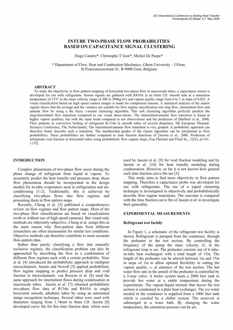
In Figure 1, a schematic of the refrigerant test facility is shown. Refrigerant is pumped from the condenser, through the preheater to the test section. By controlling the frequency of the pump the mass velocity, G, in the refrigerant loop is set. The preheater consists out of 6 tube-in-tube heat exchangers with a total length of 15m. The length of the preheater can be altered between 1m and 15m in steps of 1m to allow optimal flexibility in setting the vapour quality, x, at entrance of the test section. The hot water flow rate in the annuli of the preheater is controlled by a 3-way valve. A boiler system heats a 2000 liter tank to provide hot water at a stable temperature during the experiments. The vapour-liquid mixture that leaves the test section is condensed in a plate heat exchanger. The ice water needed in the condenser is supplied from a 1000 liter tank which is coooled by a chiller system. The reservoir is submerged in a water bath. By changing the water temperature, the saturation pressure can be set.
INTUBE TWO-PHASE FLOW PROBABILITIES
BASED ON CAPACITANCE SIGNAL CLUSTERING
Hugo Canière*, Christophe T’Joen*, Michel De Paepe*
* Department of Flow, Heat and Combustion Mechanics, Ghent University – UGent, St.Pietersnieuwstraat 41, B-9000 Gent, Belgium
ABSTRACT To study the objectivity in flow pattern mapping of horizontal two-phase flow in macroscale tubes, a capacitance sensor is
developed for use with refrigerants. Sensor signals are gathered with R410A in an 8mm I.D. smooth tube at a saturation temperature of 15°C in the mass velocity range of 200 to 500kg/m²s and vapour quality range from 0 to 1 in steps of 0.025. A visual classification based on high speed camera images is made for comparison reasons. A statistical analysis of the sensor signals shows that the average and the variance are suitable for flow regime classification into slug flow, intermittent flow and annular flow by using a the fuzzy c-means clustering algorithm. This soft clustering algorithm perfectly predicts the slug/intermittent flow transition compared to our visual observations. The intermittent/annular flow transition is found at higher vapour qualities, but with the same trend compared to our observations and the prediction of [Barbieri et al., 2008, Flow patterns in convective boiling of refrigerant R-134a in smooth tubes of several diameters, 5th European Thermal-Sciences Conference, The Netherlands]. The intermittent/annular flow transition is very gradual. A probability approach can therefore better describe such a transition. The membership grades of the cluster algorithm can be interpreted as flow probabilities. These probabilities are further compared to time fraction functions of [Jassim et al., 2008, Prediction of refrigerant void fraction in horizontal tubes using probabilistic flow regime maps, Exp.Thermal and Fluid Sc., 32(5), p1141-1155].
Figure 1: Scheme of refrigerant test facility
The test section includes an 8mm I.D. tube, a sight glass with back lightning and a high speed camera (250fps), as well as the capacitance sensor. The flow in the test section is fully developed and a constant tube diameter is assured over the full section with as little disturbances as possible.
The mass velocity of the refrigerant is measured using a coriolis type flow meter with an accuracy of ±0.2% o.r. The hot water flow rate is measured with a magnetic type flow meter with an accuracy of ±0.5% o.r. All thermocouples are of type K and insitu calibrated with an uncertainty of ±0.05°C. The uncertainty in the heat balance of the preheater is monitored online. Measurements were accepted if the uncertainty in the heat balance was smaller than ±2% (with an exceptional ±4% for G=200kg/m²s and x<0.125) and all temperature measurements of the preheater were stable within the uncertainty of ±0.05°C. The saturation temperature at exit of the preheater was controlled within ±0.5°C.
Capacitance sensor
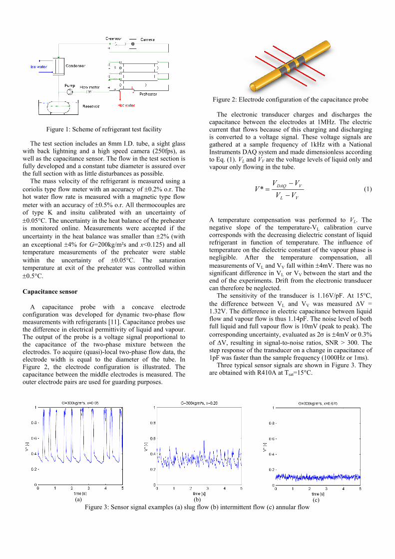
A capacitance probe with a concave electrode configuration was developed for dynamic two-phase flow measurements with refrigerants [11]. Capacitance probes use the difference in electrical permittivity of liquid and vapour. The output of the probe is a voltage signal proportional to the capacitance of the two-phase mixture between the electrodes. To acquire (quasi)-local two-phase flow data, the electrode width is equal to the diameter of the tube. In Figure 2, the electrode configuration is illustrated. The capacitance between the middle electrodes is measured. The outer electrode pairs are used for guarding purposes.
Figure 2: Electrode configuration of the capacitance probe
The electronic transducer charges and discharges the
capacitance between the electrodes at 1MHz. The electric current that flows because of this charging and discharging is converted to a voltage signal. These voltage signals are gathered at a sample frequency of 1kHz with a National Instruments DAQ system and made dimensionless according to Eq. (1). VL and VV are the voltage levels of liquid only and vapour only flowing in the tube.
VL
VDAQ
VVVV
V−
−=* (1)
A temperature compensation was performed to VL. The negative slope of the temperature-VL calibration curve corresponds with the decreasing dielectric constant of liquid refrigerant in function of temperature. The influence of temperature on the dielectric constant of the vapour phase is negligible. After the temperature compensation, all measurements of VL and VV fall within ±4mV. There was no significant difference in VL or VV between the start and the end of the experiments. Drift from the electronic transducer can therefore be neglected.
The sensitivity of the transducer is 1.16V/pF. At 15°C, the difference between VL and VV was measured ∆V = 1.32V. The difference in electric capacitance between liquid flow and vapour flow is thus 1.14pF. The noise level of both full liquid and full vapour flow is 10mV (peak to peak). The corresponding uncertainty, evaluated as 2σ is ±4mV or 0.3% of ∆V, resulting in signal-to-noise ratios, SNR > 300. The step response of the transducer on a change in capacitance of 1pF was faster than the sample frequency (1000Hz or 1ms).
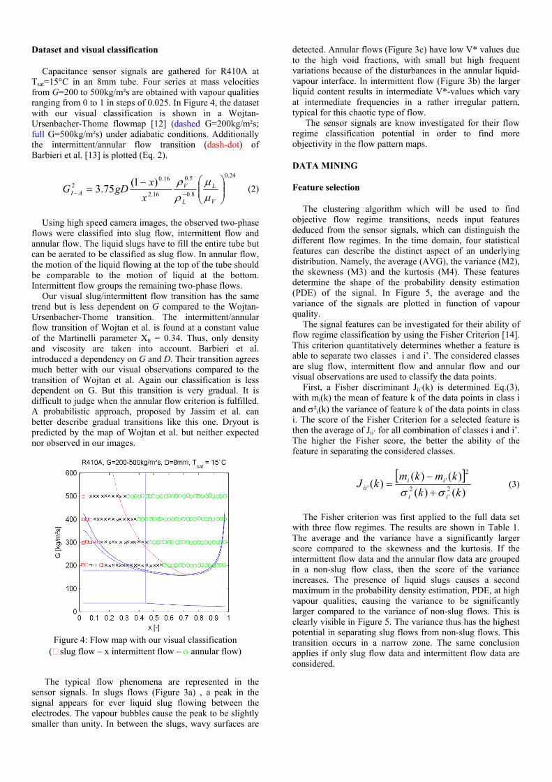
Three typical sensor signals are shown in Figure 3. They are obtained with R410A at Tsat=15°C.
Capacitance sensor signals are gathered for R410A at Tsat=15°C in an 8mm tube. Four series at mass velocities from G=200 to 500kg/m²s are obtained with vapour qualities ranging from 0 to 1 in steps of 0.025. In Figure 4, the dataset with our visual classification is shown in a Wojtan-Ursenbacher-Thome flowmap [12] (dashed G=200kg/m²s; full G=500kg/m²s) under adiabatic conditions. Additionally the intermittent/annular flow transition (dash-dot) of Barbieri et al. [13] is plotted (Eq. 2).
24.0
8.0
5.0
16.2
16.02 )1(75.3 ⎟⎟
⎠
⎞⎜⎜⎝
⎛−=
−−V
L
L
VAI x
xgDGµµ
ρρ
(2)
Using high speed camera images, the observed two-phase
flows were classified into slug flow, intermittent flow and annular flow. The liquid slugs have to fill the entire tube but can be aerated to be classified as slug flow. In annular flow, the motion of the liquid flowing at the top of the tube should be comparable to the motion of liquid at the bottom. Intermittent flow groups the remaining two-phase flows.
Our visual slug/intermittent flow transition has the same trend but is less dependent on G compared to the Wojtan-Ursenbacher-Thome transition. The intermittent/annular flow transition of Wojtan et al. is found at a constant value of the Martinelli parameter Xtt = 0.34. Thus, only density and viscosity are taken into account. Barbieri et al. introduced a dependency on G and D. Their transition agrees much better with our visual observations compared to the transition of Wojtan et al. Again our classification is less dependent on G. But this transition is very gradual. It is difficult to judge when the annular flow criterion is fulfilled. A probabilistic approach, proposed by Jassim et al. can better describe gradual transitions like this one. Dryout is predicted by the map of Wojtan et al. but neither expected nor observed in our images.
Figure 4: Flow map with our visual classification
( slug flow – x intermittent flow – ο annular flow)
The typical flow phenomena are represented in the sensor signals. In slugs flows (Figure 3a) , a peak in the signal appears for ever liquid slug flowing between the electrodes. The vapour bubbles cause the peak to be slightly smaller than unity. In between the slugs, wavy surfaces are
detected. Annular flows (Figure 3c) have low V* values due to the high void fractions, with small but high frequent variations because of the disturbances in the annular liquid-vapour interface. In intermittent flow (Figure 3b) the larger liquid content results in intermediate V*-values which vary at intermediate frequencies in a rather irregular pattern, typical for this chaotic type of flow. The sensor signals are know investigated for their flow regime classification potential in order to find more objectivity in the flow pattern maps.
DATA MINING
Feature selection
The clustering algorithm which will be used to find objective flow regime transitions, needs input features deduced from the sensor signals, which can distinguish the different flow regimes. In the time domain, four statistical features can describe the distinct aspect of an underlying distribution. Namely, the average (AVG), the variance (M2), the skewness (M3) and the kurtosis (M4). These features determine the shape of the probability density estimation (PDE) of the signal. In Figure 5, the average and the variance of the signals are plotted in function of vapour quality.
The signal features can be investigated for their ability of flow regime classification by using the Fisher Criterion [14]. This criterion quantitatively determines whether a feature is able to separate two classes i and i’. The considered classes are slug flow, intermittent flow and annular flow and our visual observations are used to classify the data points.
First, a Fisher discriminant Jii’(k) is determined Eq.(3), with mi(k) the mean of feature k of the data points in class i and σ²i(k) the variance of feature k of the data points in class i. The score of the Fisher Criterion for a selected feature is then the average of Jii’ for all combination of classes i and i’. The higher the Fisher score, the better the ability of the feature in separating the considered classes.
[ ]
)()()()(
)( 2'
2
2'
' kkkmkm
kJii
iiii σσ +
−= (3)
The Fisher criterion was first applied to the full data set
with three flow regimes. The results are shown in Table 1. The average and the variance have a significantly larger score compared to the skewness and the kurtosis. If the intermittent flow data and the annular flow data are grouped in a non-slug flow class, then the score of the variance increases. The presence of liquid slugs causes a second maximum in the probability density estimation, PDE, at high vapour qualities, causing the variance to be significantly larger compared to the variance of non-slug flows. This is clearly visible in Figure 5. The variance thus has the highest potential in separating slug flows from non-slug flows. This transition occurs in a narrow zone. The same conclusion applies if only slug flow data and intermittent flow data are considered.
(a)
(b)
Figure 5: Average (a) and variance (b) of the dimensionless sensor signals
When slug flow data and intermittent flow data are
grouped into a non-annular flow class, the average has the highest score. The same results are found when only intermittent and annular flow data are considered. In contrast with the variance, the average decreases smoothly with increasing vapour quality. No sudden change in the trend appears in the transition zone from intermittent flow to annular flow. This transition zone is broad. No single feature was found to optimally describe this transition.
The signals can further be investigated in the frequency
domain. A lot of features can be deduced, like bandwidth contribution parameters of the power density spectrum, the average power density, average frequency etc. But because a lot of scatter appears in this data, none of these parameters are found suitable for use in combination with the clustering algorithm.
Fuzzy c-means clustering algorithm [15]
A clustering algorithm is an unsupervised learning method. The goal of such a method is to deduce properties from a dataset, without the help of a supervisor providing correct answers for each observation. In the case of two-phase flow classification, no visual decisions are needed. Clustering analysis tries to group a collection of objects into subsets or clusters such that those within each cluster are more closely related to one another than objects assigned to different clusters. An object is a selection of input features deduced from a sensor signal. The choice of these input features is fundamental to the clustering technique.
The choice of a dissimilarity measure between two objects, the distance function, is a second important factor. By far the
most common choice of the distance function is the squared or Euclidian distance between two objects yj and yj’ (Eq. 4).
∑=
−=K
kkjkjkjj yywyyd
1
2'' )(),( (4)
This is a weighted average of squared feature distances
with wk the weight parameters and y the positions of the objects in feature space. Each object is iteratively assigned to one cluster based on the minimization of an objective function. Each of the weight parameters can be chosen to set the relative importance of the features upon the degree of similarity of the objects. Variables that are more relevant in separating the clusters should of course be assigned a higher influence in defining object dissimilarity.
The Fuzzy c-means clustering algorithm is a soft-clustering algorithm. This means that each data point is assigned to a cluster to some degree that is specified by a membership grade. This makes it possible to describe the boundaries between clusters in a smooth way. This membership grade MG can thus, in the case of clustering two-phase flow signals, be interpreted as flow regime probabilities. Since the aim of the signal clustering is finding a probabilistic description of flow regime boundaries, this soft-clustering algorithm is the preferred choice amongst other clustering algorithms like k-means clustering or hierarchical clustering.
Cluster classification
The output of the clustering algorithm is thus a membership grade of each class for every data point. A membership grade of unity means the sensor signal is typical for that class. The data point is assigned to the class for which it has the highest membership grade. The fuzzy c-means clustering algorithm is applied with as input features the AVG and M2. These features were selected for having the highest flow regime classification potential based on the visual classification.
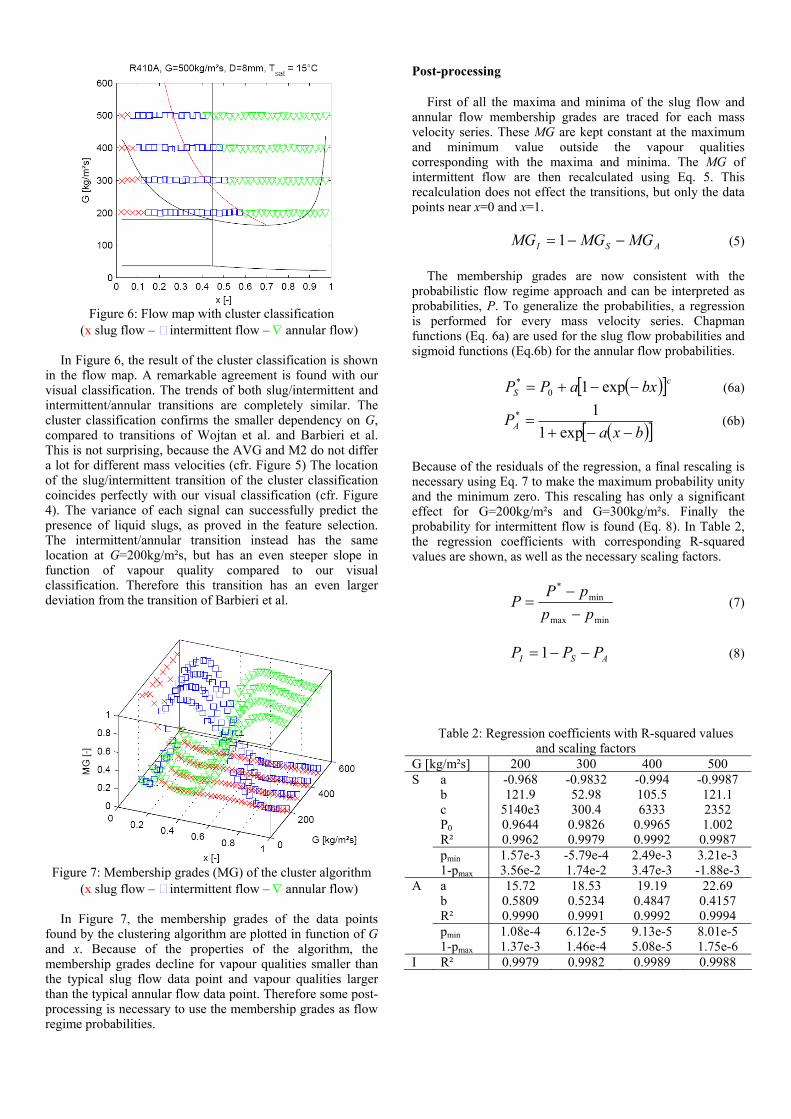
Figure 6: Flow map with cluster classification
(x slug flow – intermittent flow – ∇ annular flow) In Figure 6, the result of the cluster classification is shown
in the flow map. A remarkable agreement is found with our visual classification. The trends of both slug/intermittent and intermittent/annular transitions are completely similar. The cluster classification confirms the smaller dependency on G, compared to transitions of Wojtan et al. and Barbieri et al. This is not surprising, because the AVG and M2 do not differ a lot for different mass velocities (cfr. Figure 5) The location of the slug/intermittent transition of the cluster classification coincides perfectly with our visual classification (cfr. Figure 4). The variance of each signal can successfully predict the presence of liquid slugs, as proved in the feature selection. The intermittent/annular transition instead has the same location at G=200kg/m²s, but has an even steeper slope in function of vapour quality compared to our visual classification. Therefore this transition has an even larger deviation from the transition of Barbieri et al.
Figure 7: Membership grades (MG) of the cluster algorithm
(x slug flow – intermittent flow – ∇ annular flow) In Figure 7, the membership grades of the data points
found by the clustering algorithm are plotted in function of G and x. Because of the properties of the algorithm, the membership grades decline for vapour qualities smaller than the typical slug flow data point and vapour qualities larger than the typical annular flow data point. Therefore some post-processing is necessary to use the membership grades as flow regime probabilities.
Post-processing
First of all the maxima and minima of the slug flow and annular flow membership grades are traced for each mass velocity series. These MG are kept constant at the maximum and minimum value outside the vapour qualities corresponding with the maxima and minima. The MG of intermittent flow are then recalculated using Eq. 5. This recalculation does not effect the transitions, but only the data points near x=0 and x=1.
ASI MGMGMG −−= 1 (5)
The membership grades are now consistent with the probabilistic flow regime approach and can be interpreted as probabilities, P. To generalize the probabilities, a regression is performed for every mass velocity series. Chapman functions (Eq. 6a) are used for the slug flow probabilities and sigmoid functions (Eq.6b) for the annular flow probabilities.
( )[ ]cS bxaPP −−+= exp10
* (6a)
( )[ ]bxaPA −−+
=exp1
1* (6b)
Because of the residuals of the regression, a final rescaling is necessary using Eq. 7 to make the maximum probability unity and the minimum zero. This rescaling has only a significant effect for G=200kg/m²s and G=300kg/m²s. Finally the probability for intermittent flow is found (Eq. 8). In Table 2, the regression coefficients with corresponding R-squared values are shown, as well as the necessary scaling factors.
minmax
min*
pppPP−−
= (7)
ASI PPP −−=1 (8)
Table 2: Regression coefficients with R-squared values and scaling factors
G [kg/m²s] 200 300 400 500 S a -0.968 -0.9832 -0.994 -0.9987 b 121.9 52.98 105.5 121.1 c 5140e3 300.4 6333 2352 P0 0.9644 0.9826 0.9965 1.002 R² 0.9962 0.9979 0.9992 0.9987 pmin 1.57e-3 -5.79e-4 2.49e-3 3.21e-3 1-pmax 3.56e-2 1.74e-2 3.47e-3 -1.88e-3 A a 15.72 18.53 19.19 22.69 b 0.5809 0.5234 0.4847 0.4157 R² 0.9990 0.9991 0.9992 0.9994 pmin 1.08e-4 6.12e-5 9.13e-5 8.01e-5 1-pmax 1.37e-3 1.46e-4 5.08e-5 1.75e-6 I R² 0.9979 0.9982 0.9989 0.9988
(e)-(h) Time fraction functions of Jassim et al. [8-9] (dashed: intermittent/liquid flow, dashed-dotted: stratified, solid: annular flow)
DISCUSSION
In Figure 8, the probability functions P are plotted for the different mass velocity series (a-d). The generalized time fractions functions of Jassim et al. [8-9], evaluated for R410A in an 8mm tube at Tsat = 15°C, are plotted in Figure 8 (e-h).
It should be mentioned that the time fraction functions were developed from time fraction data with R134a at 25°C, 35°C and 50°C, R410A at 25°C, G from 100 to 400 kg/m²s, x from 0 to 1 in 8.00mm, 5.43mm and 3.90mm smooth, adiabatic, horizontal tubes [9]. The plotted time fraction functions are thus plotted for a lower temperature (15°C) and extrapolated to G=500kg/m²s. Jassim et al. considered time fractions for the intermittent/liquid, stratified and annular flow regimes. The intermittent and liquid flow regimes were grouped since the liquid flow regime was relatively insignificant. The time fraction data was obtained using an automated image recognition technique [7]. The pixel brightness at different locations in the tube was used to classify the images.
This time fraction classification thus uses different classification criteria compared to our cluster classification. For instance, they do not distinguish slug flow from intermittent flow, but consider slug flow as a combination of liquid/intermittent flow and stratified flow. Therefore, a direct comparison of the time fractions with the traditional classification (used in the flow map of Wojtan et al.) and our cluster classification is not straightforward. Nevertheless, some analogies can be drawn.
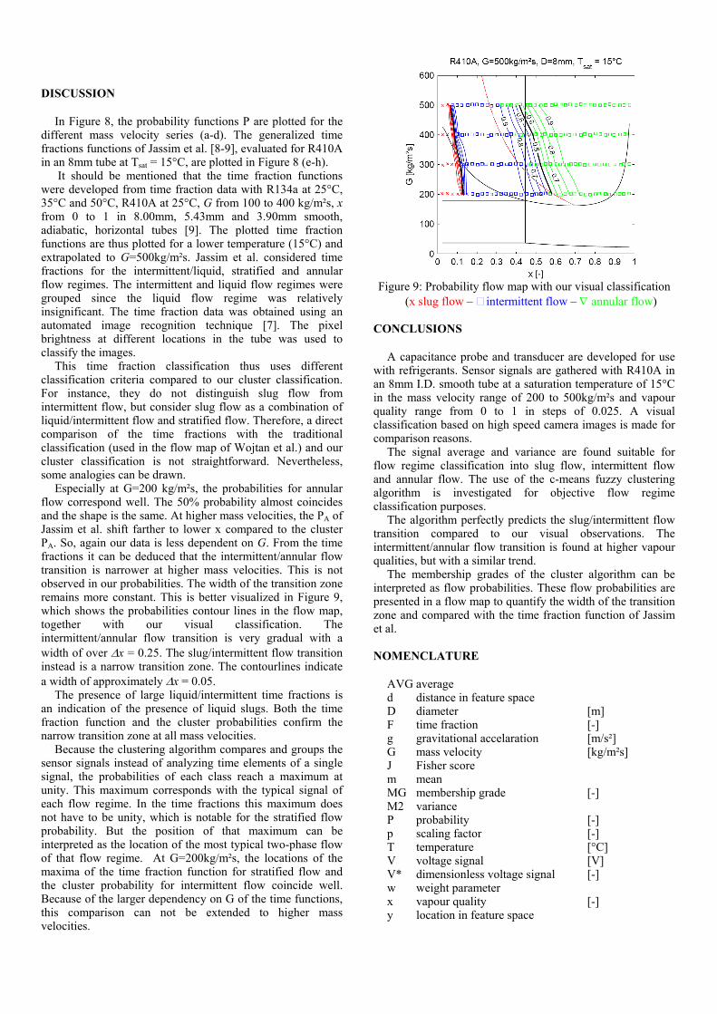
Especially at G=200 kg/m²s, the probabilities for annular flow correspond well. The 50% probability almost coincides and the shape is the same. At higher mass velocities, the PA of Jassim et al. shift farther to lower x compared to the cluster PA. So, again our data is less dependent on G. From the time fractions it can be deduced that the intermittent/annular flow transition is narrower at higher mass velocities. This is not observed in our probabilities. The width of the transition zone remains more constant. This is better visualized in Figure 9, which shows the probabilities contour lines in the flow map, together with our visual classification. The intermittent/annular flow transition is very gradual with a width of over ∆x = 0.25. The slug/intermittent flow transition instead is a narrow transition zone. The contourlines indicate a width of approximately ∆x = 0.05.
The presence of large liquid/intermittent time fractions is an indication of the presence of liquid slugs. Both the time fraction function and the cluster probabilities confirm the narrow transition zone at all mass velocities.
Because the clustering algorithm compares and groups the sensor signals instead of analyzing time elements of a single signal, the probabilities of each class reach a maximum at unity. This maximum corresponds with the typical signal of each flow regime. In the time fractions this maximum does not have to be unity, which is notable for the stratified flow probability. But the position of that maximum can be interpreted as the location of the most typical two-phase flow of that flow regime. At G=200kg/m²s, the locations of the maxima of the time fraction function for stratified flow and the cluster probability for intermittent flow coincide well. Because of the larger dependency on G of the time functions, this comparison can not be extended to higher mass velocities.
Figure 9: Probability flow map with our visual classification
A capacitance probe and transducer are developed for use with refrigerants. Sensor signals are gathered with R410A in an 8mm I.D. smooth tube at a saturation temperature of 15°C in the mass velocity range of 200 to 500kg/m²s and vapour quality range from 0 to 1 in steps of 0.025. A visual classification based on high speed camera images is made for comparison reasons.
The signal average and variance are found suitable for flow regime classification into slug flow, intermittent flow and annular flow. The use of the c-means fuzzy clustering algorithm is investigated for objective flow regime classification purposes.
The algorithm perfectly predicts the slug/intermittent flow transition compared to our visual observations. The intermittent/annular flow transition is found at higher vapour qualities, but with a similar trend.
The membership grades of the cluster algorithm can be interpreted as flow probabilities. These flow probabilities are presented in a flow map to quantify the width of the transition zone and compared with the time fraction function of Jassim et al.
NOMENCLATURE
AVG average d distance in feature space D diameter [m] F time fraction [-] g gravitational accelaration [m/s²] G mass velocity [kg/m²s] J Fisher score m mean MG membership grade [-] M2 variance P probability [-] p scaling factor [-] T temperature [°C] V voltage signal [V] V* dimensionless voltage signal [-] w weight parameter x vapour quality [-] y location in feature space
∆ difference µ dynamic viscosity [Pa s] ρ density [kg/m³] σ standard deviation σ² variance A annular flow DAQ data acquisition I intermittent flow L liquid S slug flow sat saturation V vapour
ACKNOWLEDGMENTS
The authors would like to express gratitude to the BOF fund (B/06634) of the Ghent University - UGent which provided support for this study. Special thanks to ir. L. Colman (Vakgroep Electronica, Departement Toegepaste Ingenieurswetenschappen, Hogeschool Gent, Belgium) and ir. G. Colman (Intec_Design, Department of Information Technology, Ghent University, Belgium) for the development of the capacitance transducer and to ir. B. Bauwens (Department of Electrical Engineering, Systems and Automation, UGent, Belgium) for the insights in data mining.
REFERENCES
1. J.R. Thome, Two-phase heat transfer using no-phase flow models?, Heat Transfer Eng., vol. 25, pp. 1-2, 2004.
2. L. Liebenberg and J.P. Meyer, A review of flow pattern-based predictive correlations during refrigerant condensation in horizontally smooth and enhanced tubes., Heat Transfer Eng., vol. 29, pp. 3-19, 2008.
3. L.X. Cheng, G. Ribatski and J.R. Thome, Two-phase flow patterns and flow-pattern maps: Fundamentals and applications. ASME - Appl. Mech. Rev., vol. 61, pp. 050802:1-28, 2008.
4. V. Nino, P. Hrnjak and T. Newell, Two-phase flow visualization of R134A in a multiport microchannel tube., Heat Transfer Eng., vol. 24, pp. 41-52, 2003.
5. E. Jassim and T. Newell, Prediction of two-phase pressure drop and void fraction in microchannels using probabilistic flow regime mapping, Int. J. Heat Mass Tran., vol. 49, pp. 2446-2457, 2006.
6. E. van Rooyen, M. Christians, L. Liebenberg and J.P. Meyer, Optical measurement technique for predicting time-fractions in two-phase flow. Proc. 5th Int. Conf. on Heat Transfer, Fluid Mechanics, and Thermodynamics (HEFAT), Sun City, South Africa, July 1st-4th , 2007.
7. E. Jassim, T. Newell and J. Chato, Probabilistic determination of two-phase flow regimes in horizontal tubes utilizing an automated image recognition technique., Exp. Fluids, vol. 42, pp. 563-573, 2007.
8. E. Jassim, Probabilistic flow regime map modeling of two-phase flow. Ph.D. Thesis, Urbana-Champaign, University of Illinois, IL, USA. , 2006.
9. E. Jassim, T. Newell and J. Chato, Prediction of refrigerant void fraction in horizontal tubes using probabilistic flow regime maps. Exp. Therm. Fluid Sci., vol. 32, pp. 1141-1155, 2008.
10. E. Jassim, T. Newell and J. Chato. Prediction of two-phase condensation in horizontal tubes using probabilistic flow regime maps. Int. J. Heat Mass Tran., vol. 51, pp. 485-496, 2008.
11. H. Canière, C. T’Joen, A. Willockx, M. De Paepe, M. Christians, E. van Rooyen, L. Liebenberg and J.P. Meyer, Horizontal two-phase flow characterization for small diameter tubes with a capacitance sensor, Meas. Sci. Technol., vol. 18, pp. 2898-2906, 2007.
12. L. Wojtan, T. Ursenbacher and J.R. Thome, Investigation of flow boiling in horizontal tubes: Part I - A new diabatic two-phase flow pattern map. Int. J. Heat Mass Tran., vol. 48, pp. 2955-2969, 2005.
13. P. Barbieri, J. Jabardo and E. Bandarra Filho, Flow patterns in convective boiling of refrigerant R-134a in smooth tubes of several diameters, 5th European Thermal-Sciences Conference, The Netherlands, 2008.
14. J. Shawe-Taylor and N. Cristianini, Kernel methods for pattern analysis, Cambridge University Press, Cambridge, UK, 2004.
15. J.C. Bezdek, Pattern Recognition with Fuzzy Objective Function Algorithms, Plenum Press, New York, USA, 1981.