INVARIANT MEASURES AND THEIR PROPERTIES. A …liverani/Lavori/live0203.pdf · INVARIANT MEASURES...

INVARIANT MEASURES AND THEIR PROPERTIES.

A FUNCTIONAL ANALYTIC POINT OF VIEW

CARLANGELO LIVERANI

Abstract. In this series of lectures I try to illustrate systematically what Icall the “functional analytic approach” to the study of the statistical propertiesof Dynamical Systems. The ideas are presented via a series of examples ofincreasing complexity, hoping to give in this way a feeling of the breadth ofthe method.

Contents

A foreword 21. First Lecture (the problem) 21.1. The general Problem 21.2. Existence (Kryloff–Bogoliouboff) 41.3. Why is this not enough? 41.4. A simple example: smooth expanding maps 51.5. More Regularity 71.6. Less Regularity 82. Second Lecture (three less trivial examples) 102.1. Coupled map lattices 102.2. Partially hyperbolic systems 122.3. Non-uniform expansion 143. Third Lecture (beyond existence: statistical properties) 203.1. The spectral picture 203.2. Perturbations 233.3. Differentiability of SRB-measures 264. Fourth Lecture (The uniformly hyperbolic case) 284.1. Another simple example: an attracting fixed point 284.2. The general framework 304.3. Uniformly hyperbolic systems 315. Fifth Lecture (Geodesic flows) 355.1. A bit of history 365.2. Looking at a generator 375.3. Few rough ideas about the proofs 40References 42

Date: Rome, November 18, 2002.I wish to thank the Scuola Normale Superiore, the “Center Ennio de Giorgi” and S.Marmi for

giving me the opportunity to elaborate on the point of view here presented.

1

2 CARLANGELO LIVERANI

A foreword

This text grew out of a series of five lectures that I gave at the Center Enniode Giorgi during the Research Trimester on Dynamical Systems (Pisa, February1-April 30, 2002). I must say that, while writing, I added some more material thatI felt naturally belonged to the logic of the argument but I did not have the time tocover in the actual lectures. As a consequence the present text corresponds moreto a ten rather than a five lectures course. Nevertheless, I kept the original divisionsince it is quite natural. In fact, it is rather tempting to expand the material evenfurther and make this into a full blown graduate course. I am unsure if I will ever fallfor such a temptation. In the mean time my task here is to present systematicallyan approach to the problem of statistical properties of Dynamical Systems and tryto show how far it can be carried out. This reflects my opinion that the best wayto test a point of view is to try to push it to its limits. Personally, I think that theapproach presented here may be pushed much further. For example, extending itto non uniformly hyperbolic cases or more sophisticated objects such as dynamicalζ functions. I hope that this presentation will motivate others to do so.

1. First Lecture (the problem)

This series of lectures are dedicated to the study of the statistical properties ofDynamical Systems.

I must immediately emphasize that the material and the point of view presentedhere are a bit single minded and have no intention whatsoever to constitute a reviewof the field. In fact, if one wishes to get a brief general introduction to the fieldI warmly recommend the papers by Young [91, 92] and Viana [88]; for a recentoverview on the statistical properties of Dynamical Systems see Baladi’s book [4]and [34] for a detailed general introduction to the field of Dynamical Systems.

Before starting, however, I must at least mention that the present approach has along history, beginning at least with the work of Sinai and then Ruelle, but twistedthrough the results of Lasota-Yorke and Keller, just to mention very few of themain actors.

1.1. The general Problem. Consider a Dynamical Systems (X,T ) where X is ameasurable space and T : X → X a measurable map.

The term statistical properties of a dynamical system is a very loose expressionbut it roughly relates to the properties of the evolution of measures. It is aninteresting fact of life that very complex Dynamical Systems become much simpleronce one studies the evolution of measures rather than of points.

Given a probability measure µ on X , one can define T∗µ(A) := µ(T−1A) foreach measurable set A.1 Clearly T∗ : P(X) → P(X), where P(X) is the set ofthe probability measures on X .2 Indeed, since T−1X = X , if µ ∈ P(X), thenT∗µ(X) = µ(X) = 1.

1The operator T∗ is often called Transfer operator, in analogy with the related object inStatistical Mechanics, or Perron-Frobenius operator, borrowing the terminology from the theoryof positive matrices and operators, or also Ruelle-Perron-Frobenius operator in recognition of therole of D.Ruelle in emphasizing its importance and in the study of its properties.

2In these notes we will consider only probabilities measures. Nonetheless, it must be said thatthere exists a rich and very interesting theory of σ-finite invariant measures, [1].

INVARIANT MEASURES AND THEIR PROPERTIES 3

When investigating the properties of the dynamical system (P(X), T∗), the firstrelevant question is the study of the fixed points, that is the invariant measures:µ(A) = µ(T−1A) for each measurable set A.3

Given an invariant measure µ, one can define the measurable dynamical sys-tem (X,T, µ). For such a dynamical system several natural questions concerningstatistical properties arise. The first question is the identification of the invariantsets. One of the most interesting possibilities being when all the invariant sets4

are trivial–either of zero or of full measure–such systems are called ergodic. Thiscorresponds to a study of the properties of the invariant measure itself.

If one is interested in the behavior of nearby measures, a first possibility isto consider the set A(µ) := ν ∈ P(X) | ν ≪ µ, that is the set of measuresabsolutely continuous with respect to µ. In several cases (certainly in all the onesdiscussed below) it happens that T∗A(µ) ⊂ A(µ), in this case the map is callednonsingular with respect to µ. If µ is an attractor for A(µ), then the measurabledynamical system (X,T, µ) is called mixing. This is a very interesting notion whichhas received a lot of attention due to its importance both in practical and theoreticalcontexts. For mixing systems a further obvious issue concerns the speed with whichmeasures in A(µ) are attracted to µ, the so called speed of mixing.

To understand more global properties of (P(X), T∗) one can try to gain a betterknowledge of the behavior of a larger class of measures, for example one can studythe asymptotic behavior of the measures that are absolutely continuous with respectto a given (not necessarily invariant) measure m (e.g. Lebesgue).

It is also possible to investigate stronger statistical properties of (X,T, µ) (e.g.,Central Limit Theorems, K-property, Benoully property, etc.–see [34] for a morecomplete introductory discussion). Yet, here we will limit our investigations to theabove concepts.

Of course the first question is: do invariant measures always exist?The answer is, in general, negative. Consider indeed the following two trivial

examples

(1) T : R → R defined by T (x) = x2 + 2. Clearly any invariant measure mustbe supported on [2,∞). On the other hand, if x ≥ 2, T−1x ⊂ (−∞, x− 1).Accordingly, for any bounded set A there exists n ∈ N such that T−nA ⊂(−∞, 2), hence µ(A) = µ(T−nA) = 0.5

(2) T : [0, 1] → [0, 1]

T (x) =

1

2x+

1

4∀x 6= 1

2

0 for x =1

2

Clearly, µ(1/2) = 0 since the point has no preimage. Thus letting A =[0, 1/2) ∪ (1/2, 1], for each ε > 0 there exists n ∈ N such that T nA ⊂(1/2 − ε, 1/2 + ε), so µ((1/2 − ε, 1/2 + ε)) ≥ µ(T nA) = µ(A) = µ([0, 1]).

3Notice that if T is invertible and T−1 is measurable, then the above relation is equivalent toµ(A) = µ(TA) for each measurable set A.

4That is, the measurable sets A such that T−1A ⊂ A.5Here no invariant measure at all does exist (a part from µ = 0, which clearly always exists

but we do not take into considerations since it yields no information whatsoever on the systems).If we wish to exclude only invariant probability measures, then the obvious example Tx = x+ 1suffices.


Hence, if the measure is Borel, by the regularity of the measure followsµ([0, 1]) = µ(1/2) = 0.

In the two counterexamples above the obstructions derive, in the first case, fromthe non-compactness of the space and, in the second case, from the discontinuityof the map. Essentially these are the only possible obstructions as is illustrated inthe next section.

1.2. Existence (Kryloff–Bogoliouboff).

Proposition 1.1 (Kryloff–Bogoliouboff [50]). If X is a compact metric space andT : X → X is continuous, then there exists at least one invariant (Borel) measure.

Proof. Consider any Borel probability measure ν and define the following sequenceof measures νnn∈N := T n

∗ ν. Next, define

µn =1

n

n−1∑

i=0

νi.

Again µn(X) = 1, so the sequence µi∞i=1 is contained in a weakly compact set(the unit ball) and therefore admits a weakly convergent subsequence µni

∞i=1; letµ be the weak limit.6 We claim that µ is T invariant. Since µ is a Borel measureit suffices to verify that for each f ∈ C0(X) holds µ(f T ) = µ(f). Let f be acontinuous function, then by the weak convergence we have7

µ(f T ) = limj→∞

1

nj

nj−1∑

i=0

νi(f T ) = limj→∞

1

nj

nj−1∑

i=0

ν(f T i+1)

= limj→∞

1

nj

nj−1∑

i=0

νi(f) + ν(f T nj)− ν(f)

= µ(f).

1.3. Why is this not enough? The problem with the above result is not somuch in the hypotheses of the Theorem (although discontinuous systems do havean important role in Dynamical Systems–just think of billiard systems or Poincaremaps of flows, for example) but rather in the lack of information about the invariantmeasure.

Indeed, in general there may be a lot of invariant measures and not all of themmay be relevant for the study of a system. For example, if the system has a periodicorbit T ix0ni=1, x0 ∈ X , then the Dirac measure that assigns to each point of theorbit the same weight is obviously invariant.

6This depends on the Riesz-Markov Representation Theorem that states that the space ofBorel measures M(X) is exactly the dual of the Banach space C0(X). Since the weak convergenceof measures in this case corresponds exactly to the weak-* topology, the result follows from theBanach-Alaoglu theorem stating that the unit ball of the dual of a Banach space is compact inthe weak-* topology.

7Note that it is essential that we can check invariance only on continuous functions: if we

would have to check it with respect to all bounded measurable functions we would need that µnconverges in a stronger sense (strong convergence) and this may not be true. Note as well thatthis is the only point where the continuity of T is used: to insure that f T is continuous andhence that µnj (f T ) → µ(f T ).


A simple possibility is to look for measures that are affiliated to some referencemeasure. Instead of going into some abstract discussion about a precise technicalmeaning of the word affiliated let us be very concrete and see immediately a simpleexample in which the reference measure is Lebesgue.

1.4. A simple example: smooth expanding maps. Let T be a C2(Td,Td)expanding map.8 As already mentioned we would like to restrict the measures weare interested in to measures that are related to Lebesgue. An interesting way todo so is to consider the following semi–norm

(1.1) ‖µ‖ := sup|ϕ|∞≤1

ϕ∈C1(Td,Rd)

d∑

i=1

µ(∂iϕi)

and consider the set of measures B := µ ∈ P(Td) | ‖µ‖ <∞.The next little lemma will helps us to understand what type of measures we are

considering.

Lemma 1.1. If ‖µ‖ < ∞ then µ is absolutely continuous with respect to theLebesgue measure m and, in addition, the Radon-Nykodim derivative is a functionof bounded variation.

Proof. Let µ ∈ B. For each ε ∈ (0, 1) let Jε be the smoothing operator

Jεϕ(x) :=

∫

Td

ε−dj(ε−1(x − y))ϕ(y)dy

where, j ∈ C∞(Rd,R+), supp(j) ⊂ [−1/2, 1/2]d and∫

Rd j(y)dy = 1. Moreoverdefine, as usual,

J∗εµ(ϕ) := µ(Jεϕ).

Then w-limε→0 J∗εµ = µ.9 In addition, since

Jε1 = 1, and ∂i(Jεϕ) = −Jε∂iϕ,

it holds J∗εµ(1) = µ(1) = 1 (that is J∗

ε : P(Td) → P(Td)) and

‖J∗εµ‖ = sup

|ϕ|∞≤1

ϕ∈C1(Td,Rd)

d∑

i=1

µ(Jε∂iϕi) = sup|ϕ|∞≤1

ϕ∈C1(Td,Rd)

d∑

i=1

µ(∂i(Jεϕi))

≤ sup|Jεϕ|∞≤1

ϕ∈C1(Td,Rd)

d∑

i=1

µ(∂i(Jεϕi)) = ‖µ‖(1.2)

Moreover, |J∗ε µ(ϕ)| ≤ ε−d|j|∞ |µ| |ϕ|L1 , hence J∗

εµ is absolutely continuous withrespect to Lebesgue. Let hε ∈ L∞(Td,R) be the density of J∗

ε µ. Clearly, hε ∈BV (Td,R), the space of functions of bounded variation, in addition they haveuniformly bounded variation. Accordingly, hεε>0 is a relatively compact sequence

8That is ‖DT‖ ≥ λ > 1.9By w-lim we mean the limit in the weak (or weak-∗ for the functional analytic oriented)

topology.


in L1(Td,R) ([23]). Consider any convergent subsequence hεjj∈N, and let h ∈BV (Td,R) be its limit, then for each ϕ ∈ C0(Td,R) holds

µ(ϕ) = limj→∞

J∗εjµ(ϕ) = lim

j→∞

∫

Td

hεjϕ =

∫

Td

hϕ.

Remark 1.1. Note that the closure of the space of measures with C1 density by theabove norm yields the space of measures with densities in the Sobolev space W1,1.It is an interesting exercise to check that the following holds unchanged for such aspace as well.10

The basic idea of the present approach is the realization that the operator T∗evolving the measures is a regularizing operator, if properly viewed. This is madeprecise by the following.

Lemma 1.2 (Lasota-Yorke type inequality). For each µ ∈ B holds,

T∗µ(1) = µ(1)

‖T∗µ‖ ≤ λ−1‖µ‖+Bµ(1).

Proof. We have already discussed the first inequality, for the second∑

i

T∗µ(∂iϕi) =∑

i

µ((∂iϕi) T )

=∑

i

µ(∂i((DT−1ϕ) T )i)−

∑

ij

µ(ϕj T∂i[∂jT−1i (Tx)]).

(1.3)

The result follows since

supi

|(DT−1ϕ) T )i|∞ = supi

|DT−1ϕi|∞ ≤ λ−1|ϕ|∞,

while |∑

ij µ(ϕj T∂i[∂jT−1i (Tx)]|∞ ≤ |D2T |∞d|ϕ|∞ =: B|ϕ|∞.

Lemma 1.2 readily implies that all the Kryloff-Bogoliouboff accumulations points,starting from a measure absolutely continuous with respect to the Lebesgue measurem, have density in BV (Td,R).11

Due to this state of affairs, one can study directly the evolution of the densitiesrather than the evolutions of the measures. To do so set dµ = hdx and define theoperator L : BV(Td,R) → BV(Td,R) by

Lh :=dT∗µ

dx.

A direct computation yields the well known formula

(1.4) Lf(x) =∑

y∈T−1x

| det(DyT )|−1f(y).

10In fact, changing a bit the norms (that is considering measures with densities in C1), onecan prove–with a bit more work–that the limiting object of the Kryloff-Bogoliouboff procedureare measures with C1 densities, when starting by measures in such a class. This is a nice exerciseas well.

11In fact, iterating the Lemma yields ‖Tn∗ µ‖ ≤ λ−n‖µ‖ + B(1 − λ−1)−1. The result follows

then by standard approximation arguments and the compactness of the unit ball of BV in L1

(see, e.g. the proof of Lemma 1.3).


It is an helpful exercise to redo all the above arguments directly for the operatorL. The logic is exactly the same, only one must use the BV(Td,R) norm ratherthan the ‖ ·‖ norm (which, in fact, is exactly the same, once one considers densitiesrather than measures).

A natural question is if the procedure outlined above is able to provide all theinvariant measures we may be interested in. To get a feeling of the situation justconsider the next lemma.

Lemma 1.3. For each invariant measurable set A of positive Lebesgue measurethere exists an invariant measure µ ∈ B supported in A.

Proof. Let χA be the characteristic function of the set A, and consider the measuremA(ϕ) := m(χAϕ)m(A)−1. The idea is to apply the Kryloff-Bogoliouboff procedureto mA, the problem being that mA may not belong to B (it will not if χA is not ofbounded variation). Yet, since BV is dense in L1, for each ε > 0 we can considergε ∈ BV such that

∫

gε = 1 and |χA − gε|L1 ≤ ε. Let mε(ϕ) := m(gεϕ) and let µA

and µε be weak limits of some subsequence 1nj

∑nj−1i=0 T i

∗mA and 1nj

∑nj−1i=0 T i

∗mε,

respectively. Clearly µA is supported in A. In addition, on the one hand

|µA(ϕ)− µε(ϕ)| ≤1

nj

nj−1∑

i=0

m(|χA − gε| |ϕ T i|) ≤ |ϕ|∞ε,

and, on the other hand,

‖µε‖ ≤ limj→∞

1

nj

nj−1∑

i=0

λ−i‖µε‖+B(1− λ−1)−1 = B(1− λ−1)−1.

Thus, by Lemma 1.1 it follows that there exists hε ∈ BV, for which the variation sat-isfies

∨

hε ≤ B(1−λ−1)−1, such that µε(ϕ) =∫

hεϕ. But then, by the compactnessof the unit ball of BV in L1, [23], it follows that there exists a subsequence εj suchthat hεj converges in L1 to a function of bounded variation,

∨

h ≤ B(1 − λ−1)−1.Accordingly,

µA(ϕ) =

∫

hϕ,

that is µA ∈ B.

The above lemma gives us quite a deep information on the structure of theinvariant sets of positive Lebesgue measure. For example, in the one dimensionalcase (d = 1), since h ∈ BV, its support must contain an interval, that is A mustcontain an interval. This eliminates the possibility of an invariant Cantor set ofpositive Lebesgue measure; this property is at times called local ergodicity.

The arguments in this section can be easily generalized. For example one caninvestigate cases in which the map is more or less regular.

For simplicity let us restrict our discussion to the one dimensional case (d = 1).

1.5. More Regularity. Suppose that T ∈ Cn+1(T1,T1), for n ∈ N. One can thenconsider the norms, for k ≤ n,

‖µ‖k := supϕ∈Ck

|ϕ|C0≤1

µ(ϕ(k)).


A trivial analogous of Lemma 1.1 shows that if∑n

j=0 ‖µ‖j <∞ then µ is absolutelycontinuous with respect to Lebesgue with a density n − 1 time differentiable andwith the n− 1 derivative being a bounded variation function.

It is an easy exercise to verify the formula

dk

dxk[(DT )−kϕ T ] = ϕ(k) T +

k−1∑

j=0

αj(T )ϕ(j) T,

where αj depends only on the first k− j derivatives of T . Using such a formula onecan easily generalize the computation in the proof of Lemma 1.2 whereby obtaining,for each k ≤ n,

(1.5) ‖T∗µ‖k ≤ λ−n‖µ‖k +Bk−1∑

j=0

‖µ‖j.

The above estimates give, for k = 1, the same statement of Lemma 1.2. In partic-ular, as we have already remarked,

‖Tm∗ µ‖1 ≤ B(1− λ−1)−1 ∀m ∈ N.

Using (1.5) iteratively on k one obtains, by the same token, that there exist C > 0such that

‖Tm∗ µ‖n ≤ C ∀m ∈ N.

In analogy with what we have seen so far, the above inequality implies that thereare invariant measures in Bn := µ ∈ P(X) | ∑n

i=1 ‖µ‖i <∞.

1.6. Less Regularity. There are two possibilities: maps that are only C1+α(T1,T1),α ∈ (0, 1), or maps that can have discontinuities. We will concentrate on the secondcase being more interesting.12

Let us consider the one dimensional piecewise smooth expanding case. That isa map T : [0, 1] → [0, 1] such that there exists a partition Z, in intervals, of [0, 1]

such that, for each Z ∈ Z, the map T restricted to

Z is C2. To further simplifymatters we assume strong expansivity, that is |DT | ≥ λ > 2.13 In this case we canuse the same semi-norm used for C2 maps, (1.1), that is

‖µ‖ := supϕ∈C1

|ϕ|∞≤1

µ(ϕ′).

Remark 1.2. Note that, due to the discontinuity of the map, the original Kryloff-Bogoliouboff argument 1.1 does not apply to the present situation.

To overcome such a problem we will implement the same argument of Proposition1.1 but without using the weak compactness of the measures, instead we will usethe compactness of the unit ball of the function of bounded variation in L1, [23].

Indeed, let us start by noticing the following.

12For the reader interested in the first case, consider the semi–norms:

‖µ‖α := supϕ∈C1

|ϕ|C1−α≤1

µ(ϕ′).

13In the general case in which one has only |DT | ≥ λ > 1, once must consider the powers ofthe map T in order to gain enough expansion.


Lemma 1.4. For piecewise smooth maps T∗B ⊂ A(m), the set of absolutely con-tinuous measures with respect to Lebesgue.

Proof. If ‖µ‖ < ∞, then Lemma 1.1 implies that µ is absolutely continuous withrespect to Lebesgue, it is then trivial to see that T∗µ ∈ A(m).

Accordingly, if ‖µ‖ <∞, then, for each ϕ ∈ C1,

T∗µ(ϕ′) =

∑

Z⊂Z

T∗µ(ϕ′χZ) =

∑

Z⊂Z

T∗µ(ϕ′χ

Z),

since, by Lemma 1.4, T∗µ gives zero weight to points.For each Z ∈ Z, define φZ to be linear and such that φZ = ϕ on ∂Z, then define

ψZ = ϕ− φZ , on Z, and extend ψZ to all [0, 1] by setting it equal to zero outside

Z. We obtain in this way a continuous function. Moreover, for each x ∈

Z,

|φ′Z(x)| ≤2|ϕ|∞|Z| .

Thus,

T∗µ(ϕ′) =

∑

Z⊂Z

µ(ψ′Z T ) + µ(φ′Z Tχ

Z)

≤∑

Z⊂Z

µ((ψZ T (DT )−1)′) +Bµ(1)|ϕ|∞

= µ((

∑

Z⊂Z

ψZ T (DT )−1)′)

+Bµ(1)|ϕ|∞.

We are left with the problem that the function ψ :=∑

Z⊂Z ψZ T (DT )−1 it is not

C1, in fact its derivative has a finite number of points of discontinuity. Nevertheless,for each ε we can find a continuous function gε, |gε|∞ ≤ |ψ′|∞, such that it differsfrom ψ′ only on a set of Lebesgue measure ε. Then, if we define ψε(x) := ψ(0) +∫ x

0gε(z)dz, holds |ψ − ψε|∞ ≤ 2|ψ′|∞ε. Hence,

µ(ψ′) ≤ µ(ψ′ε) + 2|ψ′|∞‖µ‖ε ≤ ‖µ‖(2|ϕ|∞ + 4|ψ′|∞ε).

Since ε is arbitrary, this implies

T∗µ(ϕ′) ≤ (2λ−1‖µ‖+B)|ϕ|∞.

We have thus, also in this case, the Lasota-Yorke inequality14

‖T∗µ‖ ≤ 2λ−1‖µ‖+B.

We can thus redo the Kryloff–Bogoliouboff argument: let µ0 ∈ B be a probabilitymeasure, then let µn := 1

n

∑n−1i=0 T

i∗µ0. By iterating the Lasota–Yorke inequality

follows

‖µn‖ ≤ 1

n

n−1∑

i=0

(2λ−1)I‖µ0‖+B(1 − 2λ−1)−1 ≤ ‖µ0‖n(1− 2λ−1)

+B

1− 2λ−1.

By Lemma 1.1 we know that the µn are absolutely continuous with respect toLebesgue and that their density hn are functions of bounded variation with uni-formly bounded variation norm. The already mentioned compactness of the unitBV ball in L1 implies that there exists a subsequence hnj

such that it converges

in L1 to a function h of bounded variation norm bounded by B(1 − 2λ−1)−1. Let

14In fact, this is the original Lasota-Yorke inequality,[62].


µ be the measure with density h, then µ ∈ B and it is trivial to check that it is aninvariant measure.

Remark 1.3. Note that we have a stronger convergence than in the usual Kryloff–Bogoliouboff argument (µnj

converges on all L∞ functions), this is an aspect of thestronger control that we must have on the system in order to control the effect ofthe discontinuities.

2. Second Lecture (three less trivial examples)

In the previous lecture we have considered only probability measures, this is avery good point of view for a probabilist but not so exciting for an analyst: the setof probability measures is not a vector space. It is natural to ask if the previousarguments can be turned into a more functional analytic setting. This will be donewhile treating the next examples. We will see in the following lectures that such afunctional analytic point of view will prove far reaching.

2.1. Coupled map lattices. Let T be a smooth expanding map of the circle.Define T : TZ → TZ as the product of such maps. Next, let Fε : TZ → TZ be adiffeomorphism close to the identity. More precisely, assume that (DFε)

−1 = Id+εAand that

|Aij | ≤ Ce−a|i−j| and |∂kAij | ≤ Ce−a|i−k|−a|j−k|.

We finally consider that map Tε := Fε T .15 Next, we want to consider an ap-propriate Banach space on which to analyze the dynamics. In analogy with theprevious lecture, let us consider the set of signed measures M(TZ) and define on itthe two norms16

|µ| := supϕ∈C0(TZ,R)|ϕ|∞≤1

µ(ϕ)

‖µ‖1 := supϕ∈C1(TZ,RZ)∑

i∈Z|ϕi|∞≤1

∑

i∈Z

µ(∂iϕi)

The first is the usual norm in M(TZ), the second is a generalization of the boundedvariation norm to the infinite dimensional setting. We will work in the space B :=µ ∈ M(TZ) | ‖µ‖1 < ∞ which is a Banach space once it is equipped with thenorm ‖ · ‖ := ‖ · ‖1 + | · |.

Let us gain some understanding of what B looks like. Given µ ∈ M(TZ) andΛ ⊂ Z we can define the marginal µΛ ∈ M(TΛ) by the relation

µ(ϕ) =: µΛ(ϕ) ∀ϕ ∈ C0(TΛ,R).

Now, if Λ is a fine set, it follows that ‖µΛ‖ <∞. We know already (Lemma 1.1) thatthis means that µΛ is absolutely continuous with respect to Lebesgue with densityof bounded variation. Accordingly, all the measures in B have finite dimensional

15The meaning of the above inequalities is that the maps are weakly coupled and the couplingis quite local, that is a motion of one coordinate is not influenced from distant coordinates, atleast for a short time.

16Actually, ‖ · ‖1 is only a semi-norm, indeed ‖ ⊗Z m‖1 = 0.


marginals which are absolutely continuous with respect to Lebesgue.17 This isclearly a natural generalization of what we have seen in the finite dimensional case.

To check that the Lasota-York inequality holds just remember equation (1.3)and notice that18

|(DTε)−1| ≤ λ−1(1 + ε(1− e−a)−1)

and∑

ij

|ϕj∂i[(DT )−1(Id + εA)ij ]|∞ ≤

∑

ij

|ϕj |∞[Bδij + ε(B + λ−1)C]e−a|i−j|

≤∑

i

|ϕi|∞[B + εC(B + λ−1)(1 − e−a)−1]

=: B1

∑

i

|ϕi|∞.

Accordingly, for ε small enough there exists θ ∈ (λ−1, 1) such that

‖Tε∗µ‖ ≤ θ‖µ‖+B1|µ|.To conclude we have a last problem: in infinite dimensions the unit ball of B is nolonger compact in L1. This is a serious problem as far as the study of the statisticalproperties is concerned (see the third lecture), one that it is not clear how to dealwith up to now. Yet, limited to the properties of the invariant measures, such astrong property it is not needed, in fact it suffices that the unit B ball is sequentiallyclosed in the weak topology. Clearly, in such a case, all the Kryloff–Bogoliouboffaccumulation point will have ‖ · ‖ norm bounded by B1(1 − θ)−1 + 1, since theiteration of the Lasota-Yorke inequality yields, for probability measures,

‖Tεn∗µ‖ ≤ θn‖µ‖+B1|(1− θ)−1µ| ≤ B1(1− θ)−1 + 1.

This implies the existence of invariant measures with finite dimensional marginalsthat are absolutely continuous with respect to Lebesgue and with BV density.

Lemma 2.1. The B unit ball is sequentially closed in the weak topology.

Proof. Let the sequence µn ⊂ B converge weakly to µ and suppose that ‖µn‖ ≤ 1.Then, for each function ϕ ∈ C1(TZ,RZ) such that

∑

i |ϕi|∞ ≤ 1, holds

∑

i∈Z

µ(∂iϕi) = liml→∞

l∑

i=−l

µ(∂iϕi) = liml→∞

limn→∞

∑

i∈Λ

µn(∂iϕi)

≤ liml→∞

limn→∞

‖µn‖l

∑

i=−l

|ϕi|∞ ≤ 1.

Hence ‖µ‖ ≤ 1.

For a generalization of the above results to the discontinuous case see [45]. In-stead consult [35, 5] for much stronger results in the smooth (analytic) case (in thelatter work a different approach, based on Statistical Mechanical methods–clusterexpansion– and pioneered in [14, 12, 13], is used).

17More is true: the bounded variation norm of the density of the Λ marginal is bounded by|Λ| ‖µ‖1, thus there is a precise control on how the measure becomes singular with respect toLebesgue as Λ increases.

18The operator norm is taken with respect to the ℓ1 vector space norm |v|1 :=∑

i∈Z|vi|.


2.2. Partially hyperbolic systems. Let us consider a partially hyperbolic system(X,T ) where X is a Riemannian compact manifold and T ∈ C2(X,X).

This means that the tangent space is naturally split into two space E0(x) ⊕Eu(x) = TxX such that19

‖DxT |Eu(x)‖ ≥ λ > 1

‖DxT |E0(x)‖ ≤ 1.

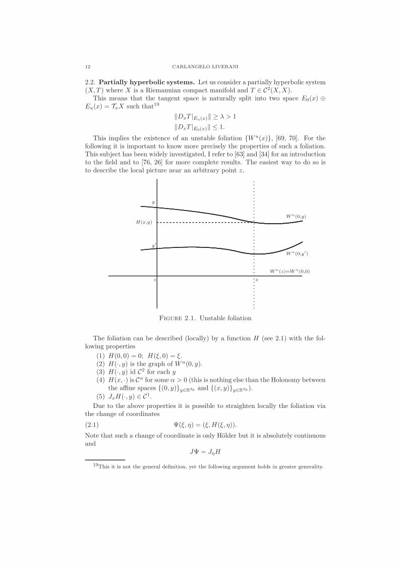
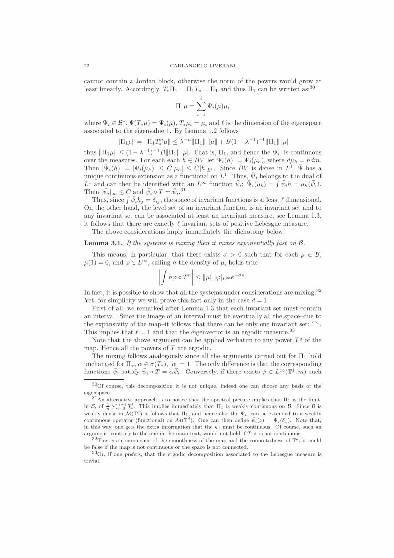
This implies the existence of an unstable foliation Wu(x), [69, 70]. For thefollowing it is important to know more precisely the properties of such a foliation.This subject has been widely investigated, I refer to [63] and [34] for an introductionto the field and to [76, 26] for more complete results. The easiest way to do so isto describe the local picture near an arbitrary point z.

x

y

y′

H(x,y)

Wu(0,y′)

Wu(0,y)

Wu(z)=Wu(0,0)

z

Figure 2.1. Unstable foliation

The foliation can be described (locally) by a function H (see 2.1) with the fol-lowing properties

(1) H(0, 0) = 0; H(ξ, 0) = ξ.(2) H(·, y) is the graph of Wu(0, y).(3) H(·, y) id C2 for each y(4) H(x, ·) is Cα for some α > 0 (this is nothing else than the Holonomy between

the affine spaces (0, y)y∈Rd0 and (x, y)y∈Rd0 ).

(5) JxH(·, y) ∈ C1.

Due to the above properties it is possible to straighten locally the foliation viathe change of coordinates

(2.1) Ψ(ξ, η) = (ξ,H(ξ, η)).

Note that such a change of coordinate is only Holder but it is absolutely continuousand

JΨ = JηH

19This it is not the general definition, yet the following argument holds in greater generality.


Let us consider the set of continuous vector fields in the unstable direction V :=v ∈ C0(X, T X) | v(x) ∈ Eu(x); smooth when restricted to unstable manifolds.The first task is to define a divergence for such vector fields

Lemma 2.2. There exists a functional u-div : V → C0(X) such that, for eachh ∈ C1, holds

(2.2)

∫

X

v(h) =

∫

X

h u-div v.

Proof. Note that (2.2) always defines a functional but, in general, we have onlyu-div v ∈ (C1)∗, our task is thus to prove the extra regularity. If v ∈ Eu(x) thenv = (w, ∂ξHw). Accordingly the vector fields in V can be described as (w, ∂ξHw)with w ∈ C1. Thus

v(h) =∑

i

wi∂xih+ (∂ξHw)i∂yi

h.

Hence, for each h ∈ C1, holds∫

v(h) =

∫

∑

i

wi∂xih+ (∂ξHw)i∂yi

h

JΨdξdη

=

∫

∑

i

wi∂ξi(h Ψ)JΨdξdη

=

∫

dη

∫

∑

i

∂ξi(wiJΨ)h Ψdξ

=

∫

h

∑

i

∂ξi(wiJΨ)(JΨ)−1

Ψ−1.

We then consider the set M(X) of signed measures on X and we define on itthe following norms20

|µ| := supϕ∈C0

|ϕ|∞≤1

µ(ϕ)

‖µ‖1 := supv∈V

|v|∞≤1

µ(u-div v).(2.3)

Not surprisingly we will restrict ourselves to B := µ ∈ M(X) | ‖µ‖1 < ∞. Thenext Lemma will give an idea of which type of measures we are talking about, butto state it properly some notation is needed. Let us consider a neighborhood Uthat can be covered by a coordinate chart of the type previously described, so thatin the new coordinates the unstable foliation consists of hyper-planes. Clearly inU the unstable foliation gives rise to a natural, measurable, partition, let us call itFu.

Lemma 2.3. ‖µ‖1 <∞ implies that, for each ϕ ∈ C0(X,R) supported in U ,21

Eµ(ϕ | Fu) = Em(hϕ | Fu)

20Again ‖ · ‖1 is a semi-norm, indeed ‖m‖1 = 0.21In the following I will use the probabilistic notation Eµ(f) for µ(f), so that I can more

naturally work with the conditional expectation E(· | Fu).


where h|Fuis BV m–a.e..

Proof. Let v be supported in a ball B ⊂ U and φ be Fu measurable. Then φ|γ =const for all γ ∈ Fu and v(φ) = 0. Then

Eµ(u-div(φv)) = Eµ(φu-div v) = Eµ(φE(u-div v | Fu)).

Taking the sup on such φ, |φ|∞ ≤ 1, we have

Eµ(|E(u-div v | Fu)|) ≤ ‖µ‖1|v|∞Hence there exists A ∈ L1(X,µ) such that

Eµ(u-div v | Fu)(x) ≤ A(x)‖µ‖1|v|∞and the lemma follows.

The above lemma characterizes the measures locally, but this suffice since it isalways possible to reduce all the considerations to small neighborhood by using asmooth partition of unity.

As an interesting example of measures in B consider

µ(ϕ) :=

∫

Wu

hϕ

where Wu is a regular piece of unstable manifold and h ∈ C1(Wu,R).Let us see how the dynamics acts on such norms.

T∗µ(ϕ) = µ(ϕ T ) ≤ |µ||ϕ|∞thus |T∗µ| ≤ |µ|.

Moreover if dµdm = h ∈ C1(X,R), then

dTn∗ µ

dm = Lnh, where the operator L is

defined by Lnh = | detDT n|−1h T−n := gnh T−n ∈ C(1)(X,R), thus

T n∗ µ(u-div v) =

∫

v(Lnh) =

∫

v(gn)

gnLnh+

∫

vn(h)

where

vn = (DT−nv) T n.

Clearly vn ∈ V and |vn|∞ ≤ λ−n|v|∞. Accordingly,

(2.4) ‖T n∗ µ‖1 ≤ λ−1‖µ‖1 +B|µ|.

This, as we have already seen, implies that there exists invariant measures in B,these are commonly called SRB (Sinai-Ruelle-Bowen) measures.22

2.3. Non-uniform expansion. The next logical step is to investigate situationsin which some non-uniform hyperbolicity takes place. In general this is a veryhard problem not yet well understood. Although many results exists ([91] for anoverview) no general theory seems to be available as yet. Here, I will discuss thesimplest possible example: a non-uniformly expanding map.

22The closeness of the unit ball of B with respect to the weak topology is left as an exercise tothe reader.


To simplify our discussion even further let us consider a very concrete family ofmaps.23 Let 0 < γ < 1 and define the map T : [0, 1] → [0, 1]

(2.5) T (x) =

x(1 + 2γxγ) ∀x ∈ [0, 1/2)

2x− 1 ∀x ∈ [1/2, 1]

This kind of maps are called intermittent and were addressed by Prellberg andSlawny in [75], they have a relationship with a statistical model introduced by Fisher[24] and then studied by Gallavotti [25]. In the papers [27], [90], the dynamicalbehavior of these maps was taken as a model for the intermittency of turbulentflows [74]. The existence of absolutely continuous invariant measures for such mapswas first proved in [86] and their statistical properties have been widely investigatedin more recent years [61, 94, 32, 95, 51, 83]. Here we will discuss only the existenceof invariant measures by adopting our present approach.

Let us consider the semi norm

‖µ‖α := supϕ(0)=0=ϕ(1)

|ϕ|C0+H0

α(ϕ)≤1

µ(ϕ′)

H0α(ϕ) := sup

x∈[0,1]

|ϕ(x)|xα

where we chose α > γ.

Lemma 2.4. The space Bα := µ ∈ M(T) | ‖µ‖α < ∞ consists of measures thatare absolutely continuous with respect to Lebesgue and with density hµ such that,setting hµ(x) := xαhµ(x), hµ ∈ L∞. In addition

|hµ|L∞ ≤ 2(α+ 2)‖µ‖α + (α+ 1)|µ|.Proof. Let µ ∈ Bα, then for each ϕ ∈ L1,

∫

[0,1]xαϕ(x) = 0, holds

∫

[0,1]

xαϕ(x)µ(dx) =

∫

[0,1]

d

dx

(∫ x

0

ξαϕ(ξ)dξ

)

µ(dx).

Now, let φ(x) :=∫ x

0ξαϕ(ξ)dξ, it is easy to see that φ(0) = φ(1) = 0, |φ|C0 ≤ |ϕ|L1 ,

Hα(φ)(0) ≤ |ϕ|L1 . Accordingly,

µ(ϕ) :=

∫

[0,1]

xαϕ(x)µ(dx) ≤ 2‖µ‖α|ϕ|L1 .

Thus, for each ϕ ∈ L1, holds, setting ϕ :=∫

xαϕ(x),

µ(ϕ) = µ(ϕ− (α + 1)ϕ) + (α+ 1)ϕµ(1) ≤ (2(α+ 2)‖µ‖α + (α+ 1)|µ|)|ϕ|L1 .

This implies that µ is absolutely continuous with respect to Lebesgue and that itsdensity hµ ∈ L∞([0, 1],m), with |hµ|∞ ≤ 2(α+ 2)‖µ‖α + (α+ 1)|µ|.

To continue we need to show that the operator enjoys some regularization prop-erty, nevertheless we cannot hope in a Lasota-Yorke type inequality as the onesalready seen. Indeed, such an inequality would imply an exponentially fast conver-gence to the invariant measure (see the next lecture) while it is known for sometime that such maps exhibits only a polinomially fast convergence to equilibrium

23One could consider more general examples (e.g. any piecewise smooth expanding maps witha finite number of neutral periodic orbits of the type T qx = x + x1+γ , γ ∈ (0, 1)) but it wouldmake little difference in the following, apart from making the exposition less readable.


[52, 66]. Nevertheless, it is possible to obtain a weaker Lasota-Yorke type inequalitywhich suffices for our purposes.

Lemma 2.5. For each α > β > γ there exist C > 0 such that

‖T n∗ µ‖α ≤ σαβ(n)‖µ‖β +Bαβ(n)|µ|, ∀n ∈ N,

where σαβ(n) := Cn−α−βγ and Bα,β(n) := Cn

(1−α)(α−β)γ(α−γ) .

Before proving such a non-uniform version of the Lasota-Yorke inequality, let ussee how it solves our problems. For each ǫ > 0 sufficiently small let αk := γ+ǫγ(1+1k ) < 1, set δk := αk+1 −αk, nk = eaǫ

−1k2

, mk :=∑k

j=1 nj , σk := σαk,αk+1(nk) and

Bk := Bαk,αk+1(nk).

24 Then for ‖µ‖γ <∞ holds

‖Tmk∗ µ‖γ+2ǫ ≤ ‖Tmk

∗ µ‖α1 ≤k∏

j=1

σj‖µ‖αk+

k−1∑

l=1

Bl

l∏

j=1

σj |µ|

≤k∏

j=1

σj‖µ‖γ +

k−1∑

l=1

Bl

l∏

j=1

σj |µ|.(2.6)

Now σk ≤ Ce−a =: σ∗ < 1, provided a has been chosen large enough. Thus∏k

j=1 σj ≤ σk∗ and

‖Tmk∗ µ‖γ+2ǫ ≤ σk

∗‖µ‖γ + C

k−1∑

j

σj∗e

1−γǫγ

a|µ| ≤ σk∗‖µ‖γ +Bε|µ|.

From the above inequality follows, in the usual way, that each invariant measureconstructed with the Kryloff-Bogoliouboff argument, starting from an absolutelycontinuous measure, will yield an invariant measure with ‖ ·‖α norm finite, for eachα > γ.

To prove Lemma 2.5 we need a good control on the distortion of the map.Let Zn be the dynamical partition of level n (that is, Zn is a maximal partition

such that T n is one-one on its elements). To have an idea of how it looks like leta0 = 1, a1 := 1/2 and an+1 := T−1an ∩ [0, 1/2]. Then [0, an] ∈ Zn.

Lemma 2.6. There exists a constant C > 0 such that

1

Cn1γ

≤ an ≤ C

n1γ

;2γ

Cγ+1n1γ+1

≤ an−1 − an ≤ Cγ+12γ

n1γ+1

.

Proof. Clearly, an+1 ≤ an. Hence

an+1 = an − 2γaγ+1n+1 ≥ an − 2γaγ+1

n ≥ 1

Cn1γ

[

1− 2γ

cγn

]

≥ 1

C(n+ 1)1γ

,

provided C is large enough.

On the other hand, for C large, a < Cn− 1γ for each an such that an − 2γaγ+1

n <2−γan. For larger n we have

an+1 = an − 2γ(an − 2γaγ+1n+1)

γ+1 ≤ an − 2γ2−γ(γ+1)aγ+1n ≤ C

(n+ 1)1γ

,

provided, again, C is large enough. Finally, the last inequality follows from thealready established ones and an−1 − an = 2γaγ+1

n .

24All this choices are largely arbitrary, many others would do as well.


Our basic distortion result is the following.25

Lemma 2.7. There exists C > 0 such that for each n ∈ N, Z ∈ Zn and x, y ∈ Zholds true

e−C

n−m+1 ≤ DxTm

DyTm≤ e

Cn−m+1 ∀m ≤ n.

Proof. For m ≤ n, holds

m−1∏

j=0

DT jxT

DT jyT≤

m−1∏

j=0

e| ln |DTjx

T |−ln |DTjy

T | ≤m−1∏

j=0

e(an−j−1−an−j)aγ−1n−j

≤ eC∑m−1

j=0 (n−j)−1− 1

γ (n−j)1− 1

γ ≤ eC∑n

j=n−m+1 j−2 ≤ eC

n−m+1 .

This concludes the proof, the other bound being completely similar.

Proof of Lemma 2.5. For each ϕ ∈ C1, holds

T n∗ µ(ϕ

′) = µ(ϕ′ T n) = µ([(DT n)−1ϕ T n]′) + µ((D2T n)(DT n)−2ϕ T n)

=: µ(φ′n) + µ(ψn).(2.7)

Note that φn is C1 on the interior of each Z ∈ Zn. In addition, φn ∈ C0 since foreach a ∈ ∂Z ∈ Zn holds T na ∈ 0, 1 hence φn(a) = 0. Nevertheless, it may notbelong to the class of test function sine it is not necessarily C1. On the other handwe have already seen in the subsection devoted to piecewise smooth maps how todeal with such a problem once it is known that the function is uniformly C1 outsidethe boundaries of the partition, so we will not replay the same argument. Thus, weneed a careful estimate of the norm of two functions φn and ψn.Estimate of the norm of φn := (DT n)−1ϕ T n. It is convenient to partitionthe orbit of x according to the time spent in a neighborhood of the fixed point.Define U0 = (0, 1/2) and let U = (0, an∗

) be a fixed neighborhood of the fixedpoint. Define n0(x) := infk ∈ N | T kx 6∈ U0. Next, let κ(x) = χU0(x)(1 −χU0(Tx)) + χU (Tx)(1 − χU (x)), clearly κ(x) is equal one if and only if the pointx enters U or exits U0 in one time step.26 We can then define ni+1(x) := infk ≥ni(x) | κ(T kx) = 1. Clearly, the stretches of trajectories between n2i and n2i+1

belong to the complement of U , while the pieces of trajectories between n2i−1 andn2i belong to U0, but starting from inside U .

Let us start analyzing a piece of trajectory in U . If z ∈ U , then T jz ∈ U foreach j < n0(z), by definition. In fact, z ∈ [an0(z), an0(z)+1]. The first interestingfact follows from Lemmata 2.6, 2.7: for each j ≤ n0(z) holds true

(2.8) DzTj ≥ C−1 an0(z)−j − an0(z)+1−j

an0(z) − an0(z)+1≥ C−3 (n0(z) + 1)

1γ+1

(n0(z)− j + 1)1γ+1.

On the other hand, outside U the map enjoys a minimal amount σ > 1 of expansionat each step.

25Here an in the following C will be used to designate fixed, possibly different, constants.26By χA we mean the characteristic function of the set A.


Clearly, the worst possible case is if all the trajectory belongs to U0, in such acase n0(x) ≥ n and

|φn(x)| ≤ C3

(

n0(x) − n+ 1

n0(x) + 1

)1+ 1γ

|ϕ(T n(x))|

≤ C3

(

n0(x) − n+ 1

n0(x) + 1

)1+ 1γ

(n0(x)− n)−αγ H0

α(ϕ)

≤ C3n0(x)−1− 1

γ (n0(x)− n+ 1)1+1−αγ H0

α(ϕ).

Maximizing on n0(x) yields

(2.9) |φn|∞ ≤ C(α)n−αγ H0

α(ϕ).

The last task is to compute the β-Holder constant of φn at zero. Let y < x, then

|φn(x)| ≤ |(DxTn)−1| |ϕ(T nx)| ≤ H0

α(ϕ)|(DxTn)−1| |T nx|α.

Again the worst possibility turns out to be the case in which all the trajectory liesin U0. In such a case, n < n0(x). Thus

|φn(x)| ≤ H0α(ϕ)

(

n0(Tnx+ 1)

n0(T nx) + n+ 1

)1+ 1γ

n0(Tnx)−

αγ (n0(T

nx) + n)βγ xβ

Taking the maximum on the possible values of n0(Tnx) yields

(2.10) Hα(φn)(0) ≤ C8(α− β)α−β

γ n−α−βγ H0

α(ϕ).

Estimate of the norm of ψn := (D2T n)(DT n)−2ϕT n. We first use the formula

(2.11) (D2xT

n)(DxTn)−2 =

n−1∑

i=0

(DxiT n−i)−1D

2xiT

DxiT

where xi := T ix. According to (2.8), if z ∈ U , then

DzTn0(z) ≥ C−3n0(z)

1γ+1 ≥ C−3n

1γ+1

∗ ≥ 2

provided we have chosen n∗ large enough. Thus in a stretch of trajectory insideU0 we get a fixed total expansion, on the other hand outside U we have some fixedamount σ > 1 of expansion at each iteration. It thus makes sense to consider astretch of trajectory in U0 as a single step. Of course, this is useful only if uniformbounds on the distortion hold. By formulae (2.11), (2.8) follows, for each z ∈ Uand m ≤ n0(z),

m−1∑

i=0

(DT izTm−i)−1D

2T izT

DT izT≤ C4

m∑

i=1

(n0(z)−m+ 1)1+1γ

(n0(z)− i)1+1γ

(n0(z)− i+ 1)−1− 1γ

= C4(n(z)−m+ 1)1+1γ

n(z)∑

i=n0(z)−m

i−2

≤ C(n(z)−m+ 1)1γ

m

n0(z).

Using the above formula one can perform the sum over the pieces of trajectoriesthat belong to U0. Accordingly, one obtains that the sum is bounded by a fixedconstant unless T nx ∈ U0. In such a case one has to analyze separately the last


terms of the sum, the one that correspond to the last run in U . Let k be the lastentrance time in U , then calling z = T kx holds n0(T

nx) = n0(z)− n+ k > 0 and

n−1∑

i=k

(DxiT n−i−1)−1D

2xiT

DxiT

≤ C

n−1∑

i=k

(

n0(z)− n+ k

n0(z)− n+ i

)1+ 1γ(

1

n0(z)− n+ i

)

γ−1γ

≤ C1(n0(z)− n+ k)1γn− k

n0(z)≤ C1n0(T

nx)1γ

1

1 + n0(Tnx)n−k

.

Accordingly, if T nx 6∈ U , we have that ψn(x) ≤ C2|ϕ|∞. On the other hand, ifT nx ∈ U , then

|ψn(x)| ≤ C1|ϕ(T nx)|n0(Tnx)

1γ

1

1 + n0(Tnx)n−k

≤ C1H0α(ϕ)n0(T

nx)1−αγ

n− k

n− k + n0(T nx)

≤ C1H0α(ϕ)n0(T

nx)1−αγ .

(2.12)

Let us consider two cases: first n0(Tnx) ≤ nδ. In such a situation we have

(2.13) |ψn(x)| ≤ C1H0α(ϕ)n

(1−α)δγ .

On the other hand, if n0(Tnx) > nδ, then let Ωk,n,m be the set of points x such

that T k−1x ∈ [1/2, 1] =: I1 and T kx ∈ [am+n−k+1, am+n−k] =: ∆m+n−k. Clearly,for x ∈ Ωk,n,m holds n0(T

nx) = m and the last entrance time in U is exactly k. LetΩ := ∪∞

m=nδ ∪nk=0Ωk,n,m, then ψn is uniformly bonded by (2.13) on the complement

of Ω. Finally, let us define ψn(x) := x−βψn(x). With such notations and using allthe above estimates we can write

µ(ψn) ≤ µ(χΩψn) + C3n(1−α)δ

γ |ϕ|Cα |µ|

≤ 3‖µ‖β + |µ||χΩψn|L1 + C3n(1−α)δ

γ H0α(ϕ)|µ|,

where we have used Lemma 2.4. We are then left with the estimate of the L1 normof χΩψn.

Clearly Ωn−k+m = T−k+1(T−1∆m+n−k ∩ I1) =: ∆m+n−k and will thus consistof an interval JZ into each element Z ∈ Zk−1. Since T k−1JZ ⊂ I1 our distortionestimates imply that

|I1||∆m+n−k|

≤ C|Z||JZ |

,

that is |JZ | ≤ C|∆m+n−k| |Z|. Let us understand a bit better how the elements ofZk−1 are distributed. For each ∆ℓ, T

ℓ∆ℓ = I1 by construction. This means that,if ℓ ≤ k

∑

Z∈Zk−1

Z⊂∆ℓ

|JZ | ≤ C∑

Z∈Zk−1

Z⊂∆ℓ

|∆m+n−k||Z| ≤ C2∑

Z′∈Zk−1−ℓ

Z′⊂I1

|∆m+n−k||Z ′||∆ℓ|

≤ C2|∆m+n−k| |∆ℓ|

where we have used again our distortion estimates.


Hence,

∫

Ω

|ψn| =∞∑

m=nδ

n∑

k=0

k∑

ℓ=1

∫

Ωm,n,k∩∆ℓ

|ψn|

≤∞∑

m=nδ

n∑

k=0

k∑

ℓ=1

C5H0α(ϕ)m

1−αγ

n− k

n− k +mℓ

βγ (m+ n− k)−

1γ−1ℓ−

1γ−1

≤ C6H0α(ϕ)

∞∑

m=nδ

n∑

k=0

m1−αγ k(m+ k)−

1γ−2

≤ C7H0α(ϕ)

∞∑

m=nδ

m−αγ ≤ C8H

0α(ϕ)n

(1−αγ)δ

Conclusion. By the above results we can estimate the terms in (2.7) as

|T ∗nµ(ϕ′)| ≤ C9n−α−β

γ + C10n(1−α

γ)δ‖µ‖β + C11n

1−αγ

δ|µ|.

We finally choose δ := α−βα−γ and the lemma follows.

3. Third Lecture (beyond existence: statistical properties)

In the previous lectures we have successfully investigated the invariant measuresof a variety of systems, still there are plenty of reasons to be unhappy about theabove considerations. A most obvious question is: what about uniqueness?

Clearly in the generality discussed so far one cannot hope that uniqueness al-ways holds. For example, consider a partially hyperbolic system consisting of anexpanding map times identity. Clearly any measure obtained by the unique ab-solutely continuous invariant measure for the expanding system times any othermeasure, on the space on which acts the identity, is an invariant measure.27

Nevertheless, in many cases it is possible to take the previous analysis muchfurther. Let us start by analyzing the simplest case: the smooth expanding maps.

3.1. The spectral picture. The idea is to use the dynamical knowledge gainedso far and transform it into informations on the spectrum of the operator T∗ on theBanach space B := complex valued measures µ such that ‖µ‖ <∞.28

First of all Lemma 1.2 implies that the spectral radius is bounded by one andthe existence of invariant measures shows that 1 ∈ σ(T∗), that is the spectral radiusis exactly one.

More can be said thanks to the following abstract result.

Theorem 3.1 (Hennion-Neussbaum argument [28]). Consider two Banach spacesB ⊂ Bw, ‖ · ‖ ≥ ‖ · ‖w, and an operator L : B → B such that, for some M > θ > 0,A,B,C > 0, and for each n ∈ N, holds true

‖Lnf‖w ≤ CMn‖f‖w; ‖Lnf‖ ≤ Aθn‖f‖+BMn‖f‖w

27It is also easy to make counterexamples by using expanding discontinuous maps, it is anhelpful exercise to try.

28Since here we want to discuss spectral theory it is convenient to consider measures andfunction with complex values. Such an extension is totally standard, thus we will not commentfurther on it.


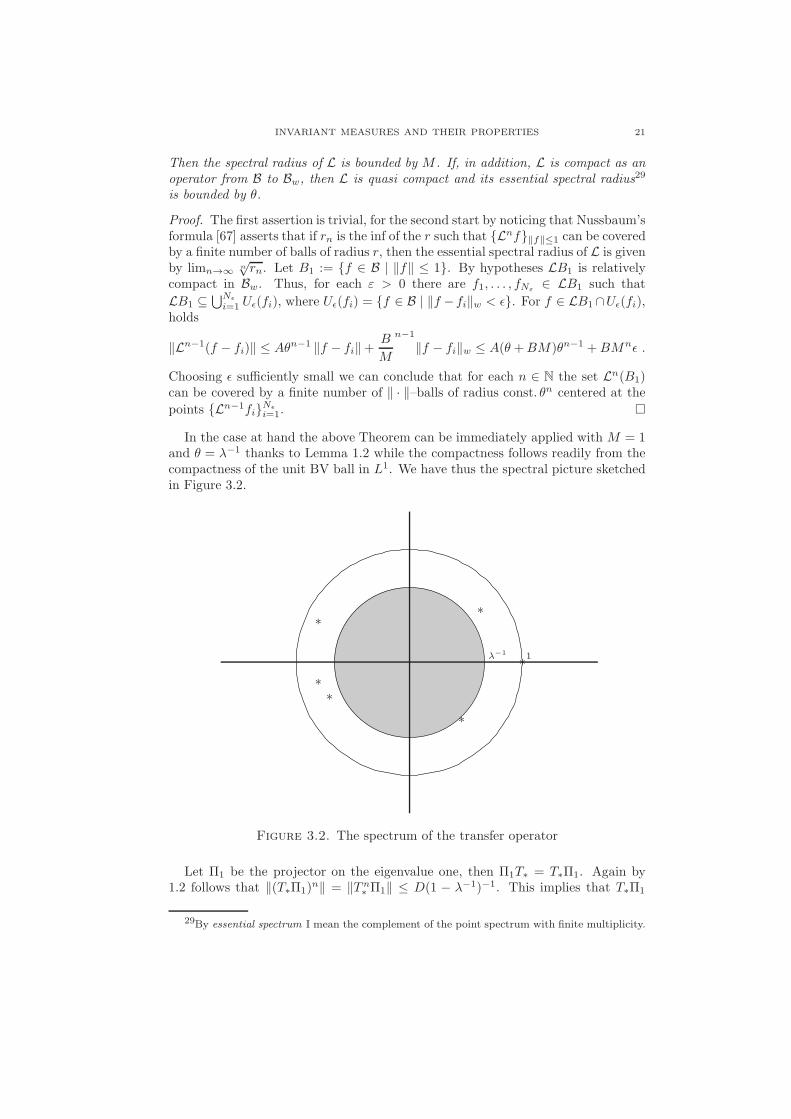
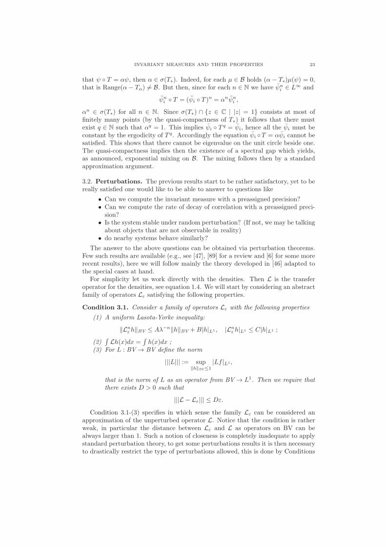
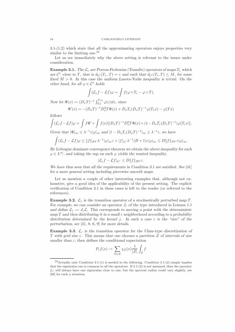
Then the spectral radius of L is bounded by M . If, in addition, L is compact as anoperator from B to Bw, then L is quasi compact and its essential spectral radius29

is bounded by θ.

Proof. The first assertion is trivial, for the second start by noticing that Nussbaum’sformula [67] asserts that if rn is the inf of the r such that Lnf‖f‖≤1 can be coveredby a finite number of balls of radius r, then the essential spectral radius of L is givenby limn→∞

n√rn. Let B1 := f ∈ B | ‖f‖ ≤ 1. By hypotheses LB1 is relatively

compact in Bw. Thus, for each ε > 0 there are f1, . . . , fNε∈ LB1 such that

LB1 ⊆ ⋃Nǫ

i=1 Uǫ(fi), where Uǫ(fi) = f ∈ B | ‖f − fi‖w < ǫ. For f ∈ LB1 ∩Uǫ(fi),holds

‖Ln−1(f − fi)‖ ≤ Aθn−1 ‖f − fi‖+B

M

n−1

‖f − fi‖w ≤ A(θ +BM)θn−1 +BMnǫ .

Choosing ǫ sufficiently small we can conclude that for each n ∈ N the set Ln(B1)can be covered by a finite number of ‖ · ‖–balls of radius const. θn centered at the

points Ln−1fiNǫ

i=1.

In the case at hand the above Theorem can be immediately applied with M = 1and θ = λ−1 thanks to Lemma 1.2 while the compactness follows readily from thecompactness of the unit BV ball in L1. We have thus the spectral picture sketchedin Figure 3.2.

1

∗∗

∗

∗∗

∗λ−1

Figure 3.2. The spectrum of the transfer operator

Let Π1 be the projector on the eigenvalue one, then Π1T∗ = T∗Π1. Again by1.2 follows that ‖(T∗Π1)

n‖ = ‖T n∗ Π1‖ ≤ D(1 − λ−1)−1. This implies that T∗Π1

29By essential spectrum I mean the complement of the point spectrum with finite multiplicity.


cannot contain a Jordan block, otherwise the norm of the powers would grow atleast linearly. Accordingly, T∗Π1 = Π1T∗ = Π1 and thus Π1 can be written as:30

Π1µ =ℓ

∑

i=1

Ψi(µ)µi

where Ψi ∈ B∗, Ψ(T∗µ) = Ψi(µ), T∗µi = µi and ℓ is the dimension of the eigenspaceassociated to the eigenvalue 1. By Lemma 1.2 follows

‖Π1µ‖ = ‖Π1Tn∗ µ‖ ≤ λ−n‖Π1‖ ‖µ‖+B(1 − λ−1)−1‖Π1‖ |µ|

thus ‖Π1µ‖ ≤ (1− λ−1)−1B‖Π1‖ |µ|. That is, Π1, and hence the Ψi, is continuousover the measures. For each each h ∈ BV let Ψi(h) := Ψi(µh), where dµh = hdm.Then |Ψi(h)| = |Ψi(µh)| ≤ C|µh| ≤ C|h|L1 . Since BV is dense in L1, Ψ has aunique continuous extension as a functional on L1. Thus, Ψi belongs to the dual ofL1 and can then be identified with an L∞ function ψi: Ψi(µh) =

∫

ψih = µh(ψi).

Then |ψi|∞ ≤ C and ψi T = ψi.31

Thus, since∫

ψihj = δij , the space of invariant functions is at least ℓ dimensional.On the other hand, the level set of an invariant function is an invariant set and toany invariant set can be associated at least an invariant measure, see Lemma 1.3,it follows that there are exactly ℓ invariant sets of positive Lebesgue measure.

The above considerations imply immediately the dichotomy below.

Lemma 3.1. If the systems is mixing then it mixes exponentially fast on B.This means, in particular, that there exists σ > 0 such that for each µ ∈ B,

µ(1) = 0, and ϕ ∈ L∞, calling h the density of µ, holds true∣

∣

∣

∣

∫

hϕ T n

∣

∣

∣

∣

≤ ‖µ‖ |ϕ|L∞e−σn.

In fact, it is possible to show that all the systems under considerations are mixing.32

Yet, for simplicity we will prove this fact only in the case d = 1.First of all, we remarked after Lemma 1.3 that each invariant set must contain

an interval. Since the image of an interval must be eventually all the space–due tothe expansivity of the map–it follows that there can be only one invariant set: T1.This implies that ℓ = 1 and that the eigenvector is an ergodic measure.33

Note that the above argument can be applied verbatim to any power T q of themap. Hence all the powers of T are ergodic.

The mixing follows analogously since all the arguments carried out for Π1 holdunchanged for Πα, α ∈ σ(T∗), |α| = 1. The only difference is that the correspondingfunctions ψi satisfy ψi T = αψi. Conversely, if there exists ψ ∈ L∞(T1,m) such

30Of course, this decomposition it is not unique, indeed one can choose any basis of theeigenspace.

31An alternative approach is to notice that the spectral picture implies that Π1 is the limit,in B, of 1

n

∑n−1i=0 T i

∗. This implies immediately that Π1 is weakly continuous on B. Since B is

weakly dense in M(Td) it follows that Π1, and hence also the Ψi, can be extended to a weaklycontinuous operator (functional) on M(Td). One can then define ψi(x) = Ψi(δx). Note that,in this way, one gets the extra information that the ψi must be continuous. Of course, such anargument, contrary to the one in the main text, would not hold if T it is not continuous.

32This is a consequence of the smoothness of the map and the connectedness of Td, it couldbe false if the map is not continuous or the space is not connected.

33Or, if one prefers, that the ergodic decomposition associated to the Lebesgue measure istrivial.


that ψ T = αψ, then α ∈ σ(T∗). Indeed, for each µ ∈ B holds (α − T∗)µ(ψ) = 0,that is Range(α− Tα) 6= B. But then, since for each n ∈ N we have ψn

i ∈ L∞ and

ψni T = (ψi T )n = αnψn

i ,

αn ∈ σ(T∗) for all n ∈ N. Since σ(T∗) ∩ z ∈ C | |z| = 1 consists at most offinitely many points (by the quasi-compactness of T∗) it follows that there mustexist q ∈ N such that αq = 1. This implies ψi T q = ψi, hence all the ψi must beconstant by the ergodicity of T q. Accordingly the equation ψi T = αψi cannot besatisfied. This shows that there cannot be eigenvalue on the unit circle beside one.The quasi-compactness implies then the existence of a spectral gap which yields,as announced, exponential mixing on B. The mixing follows then by a standardapproximation argument.

3.2. Perturbations. The previous results start to be rather satisfactory, yet to bereally satisfied one would like to be able to answer to questions like

• Can we compute the invariant measure with a preassigned precision?• Can we compute the rate of decay of correlation with a preassigned preci-sion?

• Is the system stable under random perturbation? (If not, we may be talkingabout objects that are not observable in reality)

• do nearby systems behave similarly?

The answer to the above questions can be obtained via perturbation theorems.Few such results are available (e.g., see [47], [89] for a review and [6] for some morerecent results), here we will follow mainly the theory developed in [46] adapted tothe special cases at hand.

For simplicity let us work directly with the densities. Then L is the transferoperator for the densities, see equation 1.4. We will start by considering an abstractfamily of operators Lε satisfying the following properties.

Condition 3.1. Consider a family of operators Lε with the following properties

(1) A uniform Lasota-Yorke inequality:

‖Lnεh‖BV ≤ Aλ−n‖h‖BV +B|h|L1 , |Ln

ε h|L1 ≤ C|h|L1 ;

(2)∫

Lh(x)dx =∫

h(x)dx ;(3) For L : BV → BV define the norm

|||L||| := sup‖h‖BV≤1

|Lf |L1,

that is the norm of L as an operator from BV → L1. Then we require thatthere exists D > 0 such that

|||L − Lε||| ≤ Dε.

Condition 3.1-(3) specifies in which sense the family Lε can be considered anapproximation of the unperturbed operator L. Notice that the condition is ratherweak, in particular the distance between Lε and L as operators on BV can bealways larger than 1. Such a notion of closeness is completely inadequate to applystandard perturbation theory, to get some perturbations results it is then necessaryto drastically restrict the type of perturbations allowed, this is done by Conditions


3.1-(1,2) which state that all the approximating operators enjoys properties verysimilar to the limiting one.34

Let us see immediately why the above setting is relevant to the issues underconsideration.

Example 3.1. The Lε are Perron-Frobenius (Transfer) operators of maps Tε whichare C1–close to T , that is dC1(Tε, T ) = ε and such that dC2(Tε, T ) ≤ M , for somefixed M > 0. In this case the uniform Lasota-Yorke inequality is trivial. On theother hand, for all ϕ ∈ C1 holds

∫

(Lεf − Lf)ϕ =

∫

f(ϕ Tε − ϕ T ).

Now let Φ(x) := (DxT )−1

∫ Tεx

Tx ϕ(z)dz, since

Φ′(x) = −(DxT )−1D2

xTΦ(x) +DxTε(DxT )−1ϕ(Tεx) − ϕ(Tx)

follows∫

(Lεf−Lf)ϕ =

∫

fΦ′+

∫

f(x)[(DxT )−1D2

xTΦ(x)+(1−DxTε(DxT )−1)ϕ(Tεx)].

Given that |Φ|∞ ≤ λ−1ε|ϕ|∞ and |1−DxTε(DxT )−1|∞ ≤ λ−1ε, we have

∫

(Lεf − Lf)ϕ ≤ ‖f‖BV λ−1|ϕ|∞ε+ |f |L1λ−1(B + 1)ε|ϕ|∞ ≤ D‖f‖BV ε|ϕ|∞.

By Lebesgue dominate convergence theorem we obtain the above inequality for eachϕ ∈ L∞, and taking the sup on such ϕ yields the wanted inequality.

|Lεf − Lf |L1 ≤ D‖f‖BV ε.

We have thus seen that all the requirements in Condition 3.1 are satisfied. See [41]for a more general setting including piecewise smooth maps.

Let us mention a couple of other interesting examples that, although not ex-haustive, give a good idea of the applicability of the present setting. The explicitverification of Condition 3.1 in these cases is left to the reader (or referred to thereferences).

Example 3.2. Lε is the transition operator of a stochastically perturbed map T .For example, we can consider an operator Jε of the type introduced in Lemma 1.1and define Lε := JεL. This corresponds to moving a point with the deterministicmap T and then distributing it in a small ε neighborhood according to a probabilitydistribution determined by the kernel j. In such a case ε is the “size” of theperturbation, see [41, 8, 6, 9] for more details.

Example 3.3. Lε is the transition operator for the Ulam-type discretization ofT with grid size ε. This means that one chooses a partition Z of intervals of sizesmaller than ε, then defines the conditional expectation

Pεf(x) :=∑

Z∈Z

χZ(x)1

|Z|

∫

Z

f

34Actually only Condition 3.1-(1) is needed in the following. Condition 3.1-(2) simply impliesthat the eigenvalue one is common to all the operators. If 3.1-(2) is not assumed, then the operatorLε will always have one eigenvalue close to one, but the spectral radius could vary slightly, see[60] for such a situation.


and sets Lε := PεL. The interest of such type of perturbations (discretizations)of a dynamical system lies in the fact that the range of Lε is finite dimensional.Thus the operator Lε is nothing else than a matrix. Accordingly its eigenvaluesand eigenvectors can be explicitly computed and, if they are close to the ones of theunperturbed system, this provides a possible tool for investigating the spectrum ofL itself. In fact, this strategy goes back to Ulam [87]. For more details on thisexample see [53, 41, 7, 16, 9] and for related work also [33, 64, 36, 48].

Comforted by the fact that we are talking about problems of practical interest,let us go back to our more abstract setting and see what can be done. To state theresult consider, for each operator L, the set

Vδ,r(L) := z ∈ C | |z| ≤ r or dist(z, σ(L)) ≤ δ.Since the complement of Vδ,r(L) belongs to the resolvent of L it follows that

Hδ,r(L) := sup

‖(z − L)−1‖BV | z ∈ C \Vδ,r(L)

<∞.

By R(z) and Rε(z) we will mean respectively (z − L)−1 and (z − Lε)−1.

Theorem 3.2 ([46]). Consider a family of operators Lε : BV → BV satisfyingConditions 3.1. Let Hδ,r := Hδ,r(L); Vδ,r := Vδ,r(L), r > λ−1, δ > 0, then, ifε ≤ ε1(L, r, δ), σ(Lε) ⊂ Vδ,r(L). In addition, if ε ≤ ε0(L, r, δ), there exists a > 0such that, for each z 6∈ Vδ,r, holds true

|||R(z)−Rε(z)||| ≤ Cεa.

Proof.35 To start with we collect some trivial, but very useful algebraic identities.For each operator L : BV → BV and n ∈ Z holds

1

z

n−1∑

i=0

(z−1L)i(z − L) + (z−1L)n = Id(3.1)

R(z)(z − Lε) +1

z

n−1∑

i=0

(z−1L)i(Lε − L) +R(z)(z−1L)n(Lε − L) = Id(3.2)

(z − Lε)[

Gn,ε + (z−1Lε)nR(z)

]

= Id− (z−1Lε)n(Lε − L)R(z)(3.3)

[

Gn,ε + (z−1Lε)nR(z)

]

(z − Lε) = Id− (z−1Lε)nR(z)(Lε − L),(3.4)

where we have set Gn,ε :=1z

∑n−1i=0 (z

−1Lε)i.

Let us start applying the above formulae. For each h ∈ BV and z 6∈ Vr,δ holds

‖(z−1Lε)n(Lε − L)R(z)h‖BV ≤ (rλ)−nA‖(Lε − L)R(z)h‖BV +

B

rn|(Lε − L)R(z)h|L1

≤ [(rλ)−nA2C1 +Br−nDε]Hr,δ‖h‖BV < ‖h‖BV

Thus ‖(z−1Lε)n(Lε − L)R(z)‖BV < 1 and the operator on the right hand side of

(3.3) can be inverted by the usual Neumann series. Accordingly, (z−Lε) has a welldefined right inverse. Analogously,

‖(z−1Lε)nR(z)(Lε−L)h‖BV ≤ (rλ)−nA‖R(z)(Lε−L)h‖BV+Br

−n|R(z)(Lε−L)h|L1 .

35This proof is simpler than the one in [46], yet it gives worst bounds, although sufficient forthe present purposes.


This time to continue we need some informations on the L1 norm of the resolvent.Let g ∈ BV, then equation (3.1) yields

|R(z)g|L1 ≤ 1

r

n−1∑

i=0

|(z−1L)ig|L1 + ‖R(z)(z−1L)ng‖BV

≤ 1

rn(1− r)|g|L1 +Hδ,rA(rλ)

−n‖g‖BV +Hδ,rBr−n|g|L1

≤ r−n(Hδ,rB + (1− r)−1)|g|L1 +Hδ,rA(rλ)−n‖g‖BV

Substituting, we have

‖(z−1Lε)nR(z)(Lε − L)h‖BV ≤ (rλ)−nAHδ,r2C1[1 +Br−n]

+Br−2n[Hδ,rB + (1− r)−1]Dε‖h‖BV < 1,

again, provided ε is small enough and choosing n appropriately. Hence the operatoron the right hand side of (3.4) can be inverted, thereby providing a left inverse for(z − Lε). This implies that z does not belong to the spectrum of Lε.

To investigate the second statement note that (3.2) implies

R(z)−Rε(z) =1

z

n−1∑

i=0

(z−1L)i(Lε − L)Rε(z)−R(z)(z−1L)n(Lε − L)Rε(z).

Accordingly, for each ϕ ∈ BV holds

|R(z)ϕ−Rε(z)ϕ|L1 ≤ r−n(1− r)−1ε+Hδ,r(λr)−n2AC1 +Hδ,rBε‖Rε(z)ϕ‖BV.

Remark 3.1. It takes little work to use the above Holder continuity of the spectraldata to answer the questions posed at the beginning of the section (limited to thecase of smooth piecewise expanding maps). Just remember the examples.

3.3. Differentiability of SRB-measures. The previous sections established thecontinuity of the spectral data (and of the invariant measure in particular) withrespect to various type of perturbations. It provides also an estimate of the modulusof continuity, for example for the invariant measure the modulus of continuity mustbe, at least, x ln x. Nevertheless, in certain cases, the above estimate it is notoptimal since it does not take into account extra smoothness properties of the map.Let us see how this works in our usual simple example: let us consider a C3(T1,T1)expanding map. According to our discussion in section 1.5 we can consider threenorms for the density of the measures we are interested in:

‖h‖0 := |h|L1 ; ‖h‖1 := |h|W1,1 = |h|L1+|h′|L1 ; ‖h‖2 := |h|W1,2 = |h|W1,1+|h′′|L1 ,

and the three corresponding Sobolev spaces B0 = L1(T1,R), B1 =W1,1(T1,R) and

B2 = W1,2(T1,R).36 It is easy to get the Lasota-Yorke inequality for these spaces

and the compactness of the unit ball of B1 in B0 and of B2 in B1 are well known.The application of the arguments developed so far implies that L is ergodic andhas a spectral gap both in B1 and in B2. For the perturbed family of operators letus consider, for example, a smooth random perturbation. Then we have Lεhε = hεfor the perturbed density. Let us define the quantities Lε := Lε − L; hε := hε − h.

36We choose to work with Sobolev spaces rather than with spaces of bounded variations for aprecise reason, see the discussion of equation (3.6).


By the general theory there existsM > 0 such that ‖h‖2+‖hε‖2 ≤M . In addition,Lεhε = hε implies

(Id− Lε)hε = Lεh.

Since∫

Lεh = 0 and the spectral gap implies that the spectral radius of Lε onV0

i := h ∈ Bi |∫

h = 0, i ∈ 1, 2, is strictly less than one, we can write

(3.5) hε = (Id− Lε)−1Lεh.

By the same arguments described in section 3.2 (see section 4.2 for the generalsetting) it follows that (Id − Lε)

−1 are uniformly bounded, by some constant C0,

as an operator on B1 while |||Lε|||B2→B1 ≤ Cε, hence

‖hε‖1 ≤ C0‖Lεh‖1 ≤ C0Cε‖h‖2,that is hε is Lipsichtz as a function of ε in ‖ · ‖1 norm. To get differentiability it is

necessary a bit more: the existence of an operator L : B2 → B1 such that

(3.6) limε→0

||ε−1Lεg − Lg||1 = 0 for all g ∈ B2.

Let us assume (3.6) for the time being, we will come back to it at the end ofthe section. Then, since on V0

1 (remember that by the spectral gap there existsν ∈ (0, 1) such that ‖Ln

ε ‖1 ≤ Cνn)

(Id− Lε)−1 =

∞∑

k=0

Lkε

and

|||Lkε − Lk|||B1→B0 ≤

k−1∑

j=0

|||Ljε(Lε − L)Lk−1−j |||B1→B0

≤ C

k−1∑

j=0

|||(Lε − L)Lk−1−j |||B1→B0 ≤ Cε

k−1∑

j=0

‖Lk−1−j‖1 ≤ Cεk,

it follows

|||(Id− Lε)−1 − (Id− L)−1|||V0

1→V00≤

L−1∑

k=0

|||Lkε − Lk|||B1→B0

+

∞∑

k=L

‖Ln|V01‖1 + ‖Ln

ε |V01‖1

≤ CLε+ νL ≤ Cε ln ε−1.

(3.7)

Accordingly, setting h = (Id− L)−1Lh, holds

limε→0

‖ε−1hε − h‖0 = limε→0

‖ε−1(Id− Lε)−1Lεh− (Id− L)−1Lh‖0

≤ limε→0

‖(Id− Lε)−1[ε−1Lεh− Lh]‖1 + ‖(Id− Lε)

−1Lh− (Id− L)−1Lh‖0

≤ C0 limε→0

‖ε−1Lεh− Lh‖1 = 0

which is the announced differentiability of the invariant density. To be precise wehave seen that hε ∈ C1(R,B0), as a function of ε.


Equation (3.6). Let us assume, as before, that the random perturbation is givenby Lε := JεL, where Jε is defined in Lemma 1.1. Let γ :=

∫

j(ξ)|ξ|dξ and define

Jf := γf ′. Clearly J is a bounded operator from B2 to B1.

Lemma 3.2. For each f ∈ B2 holds

limε→0

‖ε−1(Jε − Id)f − Jf‖1 = 0.

Proof. Let us start with the L1 norm. For each f ∈ C2 holds

ε−1(Jε − Id)f − Jf = −ε−1f(x) + ε−1

∫

T1

jε(x− y)f(y)dy − γf ′(x)

=

∫

T1

ε−1jε(x− y)

∫

[x,y]

f ′(z)dzdy − γf ′(x)

=

∫

T1

ε−1jε(ξ)

∫

[0,ξ]

f ′(x − η)dηdξ − γf ′(x)

=

∫

T1

dξε−1jε(ξ)

∫

[0,ξ]

f ′(x − η)− f ′(x)dη

Differentiating

d

dx[ε−1(Jε − Id)f − Jf ] =

∫

T1

dξε−1jε(ξ)

∫

[0,ξ]

f ′′(x− η)− f ′′(x)dη

Now, since f ∈ C2, both quantities inside the integrals converge everywhere to zerowhen ε → 0, and by the Lebesgue dominated convergence theorem the Lemmafollows for C2 functions. Since the above representations easily imply that ε−1(Jε−Id) are uniformly bounded operators from B2 to B1, the result for all W1,2 followsby density.37

We have thus the announced equation (3.6) setting L := JL.

4. Fourth Lecture (The uniformly hyperbolic case)

In the last lecture we have carried out our program till some of its most extremeconsequences for the case of smooth expanding maps, the next natural question is:In which generality can this program be carried out?

A part from obvious possibilities to investigate generalizations to higher dimen-sion and piecewise smooth maps (see[4] for informations on such possibilities) thefirst natural candidate are hyperbolic systems. The problem here is clearly thepresence of a stable direction. A moment thought shows that it is not clear at allhow T∗ can be seen as a regularizing operator when a stable direction is present.To understand this better let us consider the simplest possible example.

4.1. Another simple example: an attracting fixed point. Consider a mapT ∈ C2(U,U), U ⊂ Rd compact and convex. Suppose that the maps contracts:

‖DxT ‖ ≤ λ−1 ; λ > 1.

37Here finally is the difference between working with Sobolev spaces and spaces with derivativesof bounded variation. All the rest would be exactly the same but this last fact would not be trueand we could not conclude the argument. I leave this as a topic for the reader to meditate.


Clearly, such a map has only one fixed point x∗ and each smooth measure, wheniterated, converges weakly to δx∗

. So the regularity properties seem to deterioraterather than to improve.

Yet, nowhere is written that we must restrict our attention to the space ofmeasures, that is M(U) = C0(U,R)∗. Let us consider Cα(U,R)∗, α > 0, instead.More precisely, let us fix some δ > 0 and consider the norms

|ϕ|Cα := |ϕ|∞ +Hα(ϕ) ; Hα(ϕ) := sup|x−y|≤δ

|ϕ(x) − ϕ(y)||x− y|α ,

‖µ‖s,α := sup|ϕ|Cα≤1

µ(ϕ).

Then, since |ϕ T |∞ ≤ |ϕ|∞ and Hα(ϕ T ) ≤ λ−αHα(ϕ), it holds that

(4.1) ‖T∗µ‖α ≤ ‖µ‖α.

Moreover setting, for each ε > 0,

Aεϕ(x) =1

m(Bε(x))

∫

Bε(x)

ϕdm

we have, for α ∈ (0, 1),

|ϕ− Aεϕ|∞ ≤ εαHα(ϕ)

Hα(ϕ− Aεϕ) ≤ 2Hα(ϕ)

H1(Aεϕ) ≤ εα−1Hα(ϕ)

from which the Lasota-Yorke inequality follows. Indeed, for each ϕ ∈ Cα, |ϕ|Cα ≤ 1and σ ∈ (λ−α, 1), holds

T n∗ µ(ϕ) = µ(ϕ T n) = µ((ϕ − Aεϕ) T n) + µ((Aεϕ) T n)

≤ sup|φ|Cα≤(εα+2λ−nα)

µ(φ) + εα−1‖µ‖s,1 ≤ Aσn‖µ‖s,α +B‖µ‖s,1,

provided we have chosen A,B large and ε small enough. While (4.1), for α = 1,yields ‖T∗µ‖s,1 ≤ ‖µ‖s,1.

Moreover, since the unit ball of C1 is compact in Cα, it follows that the unitball of (Cα)∗ is compact in (C1)∗.38 We have thus all the ingredients to apply thestrategy outlined in the previous lecture (as it will be further remarked in the nextsection).

In particular, calling B := M(U)‖·‖s,α

and Bw := M(U)‖·‖s,1

we have thatT∗ : B → B is a quasi-compact operator and its spectral radius is one. This means

that T∗ =∑ℓ

i=1 T∗Πi +R where σ(T∗Πi) = 0, αi, |αi| = 1, and ‖Rn‖ ≤ Cθn forsome C ≥ 0 and θ < 1. But then

limn→∞

1

n

n−1∑

i=0

T i∗ = Π0,

where σ(T∗Π0) = 0, 1. Moreover, since ‖T n∗ ‖ ≤ 1 implies no Jordan blocks, it

holds true T∗Π0 = Π0T∗ = Π0.

38To see this one can, for example, apply Theorem 4.210 of [37] to the trivial embedding.


Accordingly, for each ϕ ∈ Cα and each measure µ ∈ M(U)

Π0µ(ϕ) = limn→∞

1

n

n−1∑

i=0

µ(ϕ T i) ≤ limn→∞

1

n

n−1∑

i=0

|µ| |ϕ|∞ ≤ |µ| |ϕ|∞.

This means that Π0M(U) ⊂ M(U). But the range of Π0 is finite dimensional, henceits range must be contained in M(U), since M(U) is dense in B by construction.In other words, all the µ ∈ B such that T∗µ = µ must be measures, and since thereis only one invariant measure it follows that δx∗

it is not only the unique invariantmeasure, but also the unique invariant distribution.

Remark 4.1. Note that the above arguments says nothing of interest on the regu-larity of the invariant measure (only that it is a measure, which it is obvious). Yet,it says that one can consider invariant distributions rather than invariant measuresand still be able to characterize them. This is very important if one is interested inthe the spectral picture, since eigenvectors with eigenvalue less then one are oftenonly distributions.39

4.2. The general framework. Before proceeding further it is helpful to remarkthat most of what we have done so far can be seen as special cases of a rathergeneral scheme. Such a scheme can be summarized by the following ingredients.

(1) Two Banach spaces Bi (let ‖ · ‖ be the norm of B1 and | · | the norm of B2).(2) A domination between the norms: ‖ · ‖ ≥ | · |.(3) An operator L : Bi → Bi. (L is the Transfer operator)(4) A regularization property:

‖Lnf‖ ≤ Aλ−n‖f‖+ B|f |, |Lnf | ≤ C|f |with λ > 1. (Lasota-Yorke type inequality)

(5) Compactness: Lf ∈ B1 | ‖f‖ = 1 is pre-compact in B2.(6) Invariant functional: exists ℓ ∈ B∗

2 such that L∗ℓ = ℓ.

Remark 4.2. Note that the last point corresponds, in the previous examples, to1T = 1. This is connected to our choice to restrict the analysis to measures relatedto Lebesgue. If one wants to choose a conformal measure as reference measure thenthe above setting still applies, provided it is slightly generalized. This generalizationis important (for example it is very natural to investigate the measure of maximalentropy), yet it exceeds our scopes, see [52, 4] for examples.

The consequences of the above setting are briefly summarized as follows.

• (4) =⇒ σ(L) ⊂ z ∈ C | |z| ≤ 1.• (6) =⇒ 1 ∈ σ(L).• (4,5) =⇒ σess(L) ⊂

z ∈ C

∣

∣

∣

∣

|z| ≤ λ−1

(Hennion-Neussbaum argument)

If 1 is a simple eigenvalues and no other eigenvalues of modulus one are presentthen the projection Π1 on the associated eigenvector is given by

Π1f = hℓ(f)

where Lh = h.

39As we have already remarked such eigenvalues determine the speed of decay of the correla-tions and are often called resonances [80].


Next, to consider the problems related to stability and computability, define thenorm of L seen as an operator from B1 to B2, that is

|||L||| := sup‖f‖≤1

|Lf |.

Let Li be two operators that satisfy (1-6), and

|||L1 − L2||| ≤ ε.

For any operator L, let us consider the set

Vδ,r(L) := z ∈ C | |z| ≤ r or dist(z, σ(L)) ≤ δ.Since the complement of Vδ,r(L) belongs to the resolvent of L it follows that

Hδ,r(L) := sup

‖(z − L)−1‖ | z ∈ C \Vδ,r(L)

<∞.

Theorem 4.1 ([46]). Consider two operators Li : B1 → B1 satisfying (1-6). LetHi

δ,r := Hδ,r(Li); Viδ,r := Vδ,r(Li), then there exists a, b ∈ R

+ such that, if ε ≤ε1(L1, r, δ),

‖(z − L2)−1f‖ ≤ a‖f‖+ b|f |.

In addition, setting η := ln r/αlnα−1 , if ε ≤ ε0(L1, r, δ), for each z ∈ C \V 1

δ,r it holds true

|||(z − L1)−1 − (z − L2)

−1||| ≤ εη[

a‖(z − L1)−1‖+ b‖(z − L1)

−1‖2]

.

This allows to obtain very strong spectral stability results as we have alreadyseen.

4.3. Uniformly hyperbolic systems. In this section we will consider Anosovdiffeomorphisms T : M → M where T is of class C3 and M is a smooth compactRiemannian manifold. The idea is to extend much of the results of the previouslecture to this setting. In fact, since the details starts to be a bit more technicalthis section (and the next lecture) will be less detailed. I will only try to make clearwhich type of results are possible and refer to the original papers for the completetechnical details.

Let us remind that by Anosov we mean (as usual) that there exists a direct sumdecomposition of the tangent bundle T M into continuous sub-bundles Es and Eu,that is TxM = Es

x ⊕ Eux , and constants A ≥ 1 and 0 < λs < 1 < λu such that40

(dxT )(Esx) = Es

Tx, ‖(dxT n)|Esx‖ ≤ Aλns ,

(dxT )(Eux ) = Eu

Tx, ‖(dxT−n)|Eux‖ ≤ Aλ−n

u ,(4.2)

for all x ∈ M and n ≥ 0. Let du/s = dim(Eu/s). It is well known that for such mapsthere exist stable and unstable foliations (W s(x))x∈M and (Wu(x))x∈M, [34, 63, 29].

Each single W s/u(x) is an immersed C3 sub-manifold of M, and TyW s/u(x) = Es/uy

for any y ∈ W s/u(x). The dependence of Es/ux and W s/u(x) on x, however, is only

Holder in general–see [76, 26] for exact results. We will denote by τ the optimalcommon Holder-exponent for both distributions. This exponent depends in a wellunderstood way on the various contraction and expansion coefficients of the map,and there are a number of cases where the foliations are indeed C1+α for some α > 0(for example when dim(M) = 2).

40By dT we denote the differential of T , clearly dxT : TxM → TTxM. Similarly, if f : M → R isdifferentiable, then dxf : TxM → R.


It is immediate to verify that, if µ is absolutely continuous with respect to theRiemannian volume m, then T∗µ is absolutely continuous with respect to m. Giventhis fact, it is possible to define the evolution of the corresponding densities:

L dµ

dm:=

d(T∗µ)

dm.

The above defined operator L is usually called the Perron-Frobenius or the Ruelle-Perron-Frobenius or the Transfer operator.

A direct computation shows that L has the following representation:

(4.3) Lf = f T−1 · d(T∗m)

dm=: f T−1 · g ∀f ∈ L1(M,m)

where g ∈ C2(M).41

To treat this case we will try to combine the approaches that were successful inthe expanding case and the one that worked in the contracting case. We start bydefining a suitable set of test functions to control the stable direction. For pointsx, y ∈ M with y ∈ W s(x) we define ds(x, y) as the distance between x and y withinthe Riemannian manifold W s(x) (which inherits its Riemannian structure from M).Fix some δ > 0. For 0 < β ≤ 1 and bounded measurable ϕ : M → R, we define42

(4.4) Hsβ(ϕ) := sup

ds(x,y)≤δ

|ϕ(x) − ϕ(y)|ds(x, y)β

,

which means that the supremum is taken over all pairs of points x and y such thaty ∈ W s(x). Clearly, Hs

β is a semi norm, and we use it to define

(4.5) Dβ := ϕ : M → R : ϕ measurable, |ϕ|∞ ≤ 1, Hsβ(ϕ) ≤ 1.

In order to control the unstable direction we provide a set V of measurabletest vector fields v : M → T M adapted to the unstable foliation in the sense thatv(x) ∈ Eu

x for all x ∈ M.Given the fact that x 7→ Eu

x is, in general, only τ -Holder for some τ < 1 wecannot ask the vector fields to be globally more regular than that. By a slightabuse of notation we define43

(4.6) Hsβ(v) := sup

d(x,y)s≤δ

‖v(x) − v(y)‖ds(x, y)β

.

Then we will consider the vector fields

(4.7) Vβ := v ∈ V : |v|∞ ≤ 1; Hsβ(v) ≤ 1 .

From now on we will always assume

0 < β < γ ≤ 1 .

41If M = Td then g = |det(DT )|−1.42The δ in the definition is fixed once and for all, yet it must satisfy various smallness require-

ments that depend only on (M, T ).43To compute the difference between two tangent vectors at different (close) points we parallel

transport one of them to the tangent space of the other along the geodesic. We will not mentionthis explicitly, since it is completely trivial on M = Td and it is a routine operation on generalRiemannian manifolds, see e.g. [18, Section 2.3].


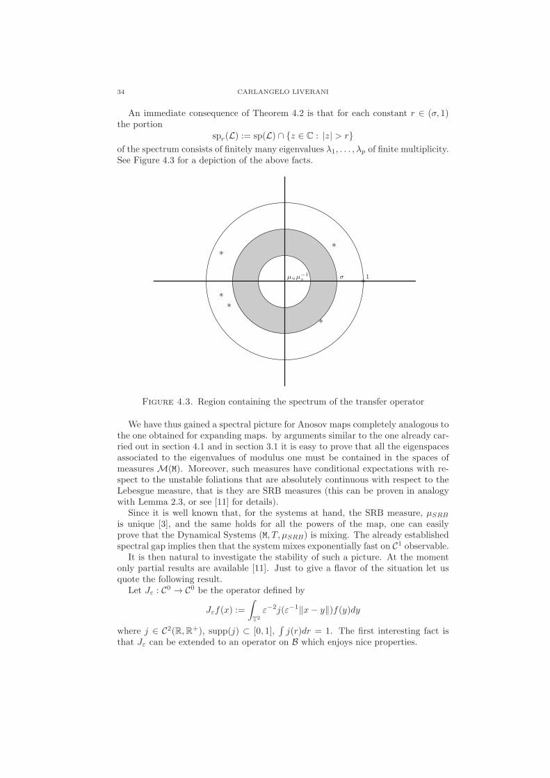
Using the above defined classes of test functions and test vector fields we nowdefine the norms that will describe our Banach spaces of generalized functions. Forf ∈ C1(M,R) let

(4.8)

‖f‖s := supϕ∈Dβ

∫

Mfϕ dm

‖f‖u := supv∈Vβ

∫

Mdf(v)dm

‖f‖ := ‖f‖u + b‖f‖s‖f‖w := sup

ϕ∈Dγ

∫

Mfϕ dm.

where∫

Mdf(v)dm is short hand for

∫

Mdxf(v(x))m(dx). The constant b ≥ 1 must

be chosen sufficiently large. Except for ‖ · ‖u, which is only a semi norm, allthese expressions define norms on C1(M,R) and ‖f‖w ≤ ‖f‖s ≤ b−1‖f‖. Note thatthe above norms are inhomogeniously anisotropic because the stable and unstabledirections are treated differently and may change from point to point.

Definition 4.1. B(M) and Bw(M) denote the completions of C1(M,R) w.r.t. thenorms ‖ · ‖ and ‖ · ‖w, respectively.

Each f ∈ C1(M,R) naturally gives rise to a bounded linear functional on C1(M,R)by virtue of

〈f, ϕ〉 :=∫

M

fϕ dm .

Obviously, ‖f‖∗C1 ≤ ‖f‖w ≤ ‖f‖ ≤ ‖f‖C1. Therefore there exist canonical continu-ous embedding (not necessarily one-to-one)

C1(M,R) → B(M) → Bw(M) → C1(M,R)∗ .

In fact, each f ∈ Bw defines a bounded linear functional on C1(M,R) by 〈f, ϕ〉 :=limn→∞〈fn, ϕ〉 where fn ∈ C1(M,R) and limn→∞ ‖f − fn‖w = 0. In the same wayone can embed B(M) into Bw(M).

We now state, without proof, the two basic fact that hold true in (and justifythe) above setting.

Lemma 4.1 ([11]). Suppose β < minτ, 1 and γ ∈ (β, 1]. Then L extends natu-rally to a bounded linear operator on both Bw(M) and B(M). In addition, for eachσ > maxλ−1

u , λβs , we can choose constants b and δ in (4.4) - (4.8) for which thereexists B > 0 such that, for each f ∈ B(M), we have

‖Lnf‖w ≤ A ‖f‖w and ‖Lnf‖ ≤ 3A2σn‖f‖+B‖f‖w for n = 1, 2, . . .

where A is the constant from (4.2).

Proposition 4.1 ([11]). If γ ·minτ, 1 > β, then the ball B1 := f ∈ B(M) : ‖f‖ ≤1 is relatively compact in Bw(M).

The next Theorem follows by the usual Hennion-Neussbaum argument.

Theorem 4.2. Suppose that γ ·minτ, 1 > β. Then, for each σ > maxλ−1u , λβs ,

the operator L : B(M) → B(M) has essential spectral radius bounded by σ and is thusquasi compact.


An immediate consequence of Theorem 4.2 is that for each constant r ∈ (σ, 1)the portion

spr(L) := sp(L) ∩ z ∈ C : |z| > rof the spectrum consists of finitely many eigenvalues λ1, . . . , λp of finite multiplicity.See Figure 4.3 for a depiction of the above facts.

1

∗∗

∗

∗∗

∗µuµ−1s σ

Figure 4.3. Region containing the spectrum of the transfer operator

We have thus gained a spectral picture for Anosov maps completely analogous tothe one obtained for expanding maps. by arguments similar to the one already car-ried out in section 4.1 and in section 3.1 it is easy to prove that all the eigenspacesassociated to the eigenvalues of modulus one must be contained in the spaces ofmeasures M(M). Moreover, such measures have conditional expectations with re-spect to the unstable foliations that are absolutely continuous with respect to theLebesgue measure, that is they are SRB measures (this can be proven in analogywith Lemma 2.3, or see [11] for details).

Since it is well known that, for the systems at hand, the SRB measure, µSRB

is unique [3], and the same holds for all the powers of the map, one can easilyprove that the Dynamical Systems (M, T, µSRB) is mixing. The already establishedspectral gap implies then that the system mixes exponentially fast on C1 observable.

It is then natural to investigate the stability of such a picture. At the momentonly partial results are available [11]. Just to give a flavor of the situation let usquote the following result.

Let Jε : C0 → C0 be the operator defined by

Jεf(x) :=

∫

T2

ε−2j(ε−1‖x− y‖)f(y)dy

where j ∈ C2(R,R+), supp(j) ⊂ [0, 1],∫

j(r)dr = 1. The first interesting fact isthat Jε can be extended to an operator on B which enjoys nice properties.


Lemma 4.2. Assume that M = T2. The unstable foliation is Cτ , τ − 1 ≥ α ≥ γ >β > 0. Then any smooth averaging operator can be extended in a unique way to acontinuous operator on B(M) and one can choose δ (small) and b (large) in such away that there exists K > 0 with

‖Jε‖w ≤ K and ‖Jεf‖ ≤ 3‖f‖+K‖f‖wfor all sufficiently small ε > 0 and all f ∈ B(M).

We can then define the operator Lε := JεL. As already noticed Lε is the transferoperator of a random process consisting in moving a point by the map T followedby a random jump determined by the transition kernel Jε. In other words at eachstep of time the point is displaced at random in a small neighborhood of its currentposition, thus we have a small random perturbation of the deterministic system.The goal is clearly to apply the perturbation theory described in the previouslecture. This is possible thanks to the next two results.

Lemma 4.3 ([11]). Assume that M = T2. There is a constant B′ > 0 such that,for sufficiently small ε > 0 and each n ∈ N

‖Lnε ‖w ≤ B′ and ‖Ln

ε f‖ ≤ 9A2σn‖f‖+B′‖f‖wfor all f ∈ B(M).Lemma 4.4 ([11]). Assume that M = T2. There exists a constant K > 0 such that

|||Jε − Id||| ≤ Kεγ−β.

Accordingly |||Lε − L||| ≤ ‖L‖Kεγ−β which suffice to apply Theorem 4.1 andobtain the wanted spectral stability.44

5. Fifth Lecture (Geodesic flows)

In this last lecture we will discuss flows. Since some aspect are a bit technical–although very similar to what we have discussed already–I will mostly restrict tothe ideas referring to the original article [58] for the nasty details.

We will consider a C4, d+ 1 dimensional, connected compact Riemannian man-ifold M with everywhere negative curvature and the associated geodesic flow45 onthe unitary tangent bundle M. The flow Tt : M → M so defined satisfies the followingconditions.

Lemma 5.1 ([49]). At each point x ∈ M there exists a splitting of the tangent spaceTxM = Es(x) ⊕ E0(x) ⊕ Eu(x). The splitting is invariant with respect to Tt, E

0

is one dimensional and coincides with the flow direction, in addition there existsµ > 0 such that

‖dTtv‖ ≤ e−µt‖v‖ for each v ∈ Es and t ≥ 0

‖dTtv‖ ≥ eµt‖v‖ for each v ∈ Eu and t ≤ 0.

44Note that the above estimates imply only Holder continuity in ε even for the SRB measure.This is a consequence of the choice of the spaces. The situation could be improved in the twodimensional case, since the foliation is, in this case, C1+α regular but for the higher dimensionalcase where the foliation can be only Holder continuous it is not clear how to improve the aboveapproach. Nevertheless, it is known that the SRB measure is differentiable in quite generalsituations [81, 82, 22], so it is clear that more work is needed to understand the real potentialityof the present point of view.

45That is T0 = Id and Tt+s = Tt Ts for each t, s ∈ R.


That is, the flow is Anosov.46

Remark 5.1. We will restrict our discussion geodesic flows but all is said holdsmore generally for contact flows.47

5.1. A bit of history. For geodesic flows (and contact flows as well) the Riemann-ian volume (contact volume) is invariant, hence the issue of finding “nice” invariantmeasure is trivial.48 On the contrary the investigation of the statistical propertiesof the flow are far from trivial. Here is a bit of history of the subject.

Although the interest in geodesic flows is very old, for convenience we can startour history with Hopf who in 1939 proved the ergodicity of geodesic flows on surfacesof constant negative curvature, [30, 31]. His argument, to this days called the Hopfargument, proved a very far reaching tool to investigate ergodicity in hyperbolicsystems (see [59] for a modern application of such ideas). The mixing of suchsystems was proved by Sinai [85] in 1961.

The next step was undertaken by Anosov in 1963, [2]. He proved ergodicity ofgeodesic flows in negative curvature. Thanks to his work it was possible to extendthe Hopf strategy to the a large class of systems (not by chance now called Anosov)even when the stable and unstable foliation are not C1. This was an impressivetechnical advance. After about ten years Ornstein and Weiss [68] established thatthis more general class of systems was mixing (in fact Bernoulli).

The study of the rate of mixing starts with the work of Collet, Epstein, Gallavottiin 1984, [17] soon followed by other similar results [65, 77, 71]. In these papers it isproven the exponential decay of correlations for geodesic flows in constant negativecurvature (in two and three dimensions). Unfortunately, the technique used thereare based on representation theory and therefore use in an essential way the groupstructure of the constant curvature case.

The possibility to obtain a more dynamical proof of the rate of decay of correla-tion came about thanks to the monumental work of Sinai, Ruelle and Bowen thatdeveloped the so called thermodynamic formalism for Dynamical Systems (see [34]for a review of such theory). This approach was extend to flows in a sequence ofworks [84, 79, 73].

Building on such foundations Chernov in 1998 was finally able to produce a dy-namical approach to the study of decay of correlation for flows, [15]. He managedto prove sub-exponential decay of correlations for geodesic flows on negative cur-vature surfaces. Shortly after Dolgopyat, in a series of papers [19, 20, 21], provedexponential decay of correlations for Anosov flows in negative curvature with C1

foliations (e.g.: negative curvature surfaces and 1/4-pinched manifolds).At this point the reader may guess that all axion A flows enjoy exponential decay

of correlations for smooth observable, this turns out to be false. Indeed, Ruelle in1983 produced an example of a suspension over a shift with piecewise constantceiling which it is mixing but exhibits arbitrarily slow correlation decay, [79] (seealso [72]). Such an example is not Anosov, yet it is hyperbolic (Axiom A). To this

46More in general, one can allow a constant A > 0 in front of the exponential term, but thiscan be handled exactly as in the following.

47By contact flow we mean that there exists a C(2) one form α on M, such that there exists aC(2) one form α on M, such that α ∧ (dα)d is nowhere zero, which is left invariant by Tt (that isα(dTtv) = α(v) for each t ∈ R and tangent vector v ∈ T M).

48Yet, there exists other very important invariant measures that one may be interest in inves-tigating such as the measure of maximal entropy.


days it is not known if all Anosov flows mixes exponentially fast, yet we are goingto see that this is the case for contact Anosov flows.

5.2. Looking at a generator. We can now start to describe the spaces on whichwe will consider the operators Tt and Lt.

49 First of all let us fix δ > 0 sufficientlysmall and define

(5.1) Hs,β(ϕ) := supds(x,y)≤δ

|ϕ(x) − ϕ(y)|ds(x, y)β

; |ϕ|s,β := |ϕ|∞ +Hs,β(ϕ).

Definition 5.1. In the following by the Banach space Cαs (M,C) we will mean the

closure of C1(M,C) with respect to the norm | · |s,α. Similar definitions hold withrespect to the metric du and the Riemannian metric d (giving the space of Holderfunction Cα).

Let us also define the unit ball Dβ := ϕ ∈ Cβs (M,C) | |ϕ|s,β ≤ 1. For a given

β < 1, and f ∈ C1(M,C), let

(5.2)

‖f‖w := supϕ∈D1

∫

Mϕf

‖f‖ := ‖f‖s + ‖f‖u ; ‖f‖s := supϕ∈Dβ

∫

Mϕf ; ‖f‖u := Hu,β(f).

Let B(M,C) and Bw(M,C) be the completion of C1(M,C) with respect to the norms‖ · ‖ and ‖ · ‖w respectively. Note that such spaces are separable by constructionand are all contained in (Cβ)∗, the dual of the β-Holder functions.

It is well known that the strong stable and unstable foliations and the Jacobianof the holonomies associated to the stable and unstable foliations for an Anosovflow are τ -Holder. From now on we will assume

(5.3) 0 < β < τ2.

Again it is possible to prove some regularization properties of the family Lt.

Lemma 5.2 (Lasota-Yorke type inequality). Ltt≥0 is a strongly continuous semigroup on B and Bw. In addition,

‖Ltf‖w ≤ ‖f‖w ; ‖Ltf‖ ≤ ‖f‖‖Ltf‖ ≤ 3e−λβt‖f‖+B‖f‖w.

Hence there exists a generator X : D(X) ⊂ B → B and the following formulafor the resolvent holds true

(z −X)−1 = R(z) =

∫ ∞

0

e−ztLtdt ; ∀z ∈ C,ℜ(z) > 0.

Unfortunately the unit ball of B it is not compact in Bw. This is due to theobvious fact that our norms do not induce any control on the flow direction. Nev-ertheless, the above formula it is very inspiring since the operator R(z) can bewritten as an integral along the flow direction, it is thus not inconceivable thatthe range of R(z) be regular also in the flow direction, whereby yielding somecompactness property.

49Clearly Lt is defined by∫Mϕ Tthdm =

∫MϕLthdm.


Lemma 5.3. Let z = a+ ib, a > 0, then

‖R(z)‖w ≤ a−1 ; ‖R(z)‖ ≤ a−1

‖R(z)nf‖ ≤ 3

(a+ λβ)n‖f‖+ a−nB‖f‖w.

In addition, R(z) : B(M,C) → Bw(M,C) is compact.

We can then investigate the spectrum of X by studying the resolvent.Note that ζ ∈ ρ(R(z)) is equivalent to z − ζ−1 ∈ ρ(X). Thus the bound on

the spectral radius of R(z) implies that σ(X) lies in the left half plane (see Figure5.4). This information is of little interest (it followed already from the fact that Lt

is bounded in the future). On the other hand, Lemma 5.3 implies, via the usualarguments (see Theorem 3.1) the quasi compactness of R(z). This means that onecan get some information on the spectrum of X on the left of the imaginary axis(see Figure 5.5). In fact, by varying z, it follows that there is a strip on the left ofthe imaginary axis that contains only point spectrum of finite multiplicity withoutaccumulation points (see Figure 5.6).

a−1=⇒

♣ z

σ(R(z))

σ(X)c

Figure 5.4. Relation between the spectral radius of R(z) and σ(X).

a−1=⇒

♣ z

σ(R(z))

∗

∗

∗

∗

∗

∗

Figure 5.5. Relation between the quasi compactness of R(z) and σ(X)

By arguments similar to the one seen for expanding maps the ergodicity of theflow implies that 0 is a simple eigenvalue, while the mixing implies σ(X)∩ibb∈R =0.Remark 5.2. Up to now the results hold for each Anosov flow and they correspondto the to the existence of a strip on which the Laplace transform of the correlationfunctions (or the dynamical zeta function) is meromorphyc.

Yet, we cannot conclude much about decay of correlations from the above results.The obstacle is that, although the imaginary axis is free of eigenvalues (apart from


∗

∗

∗

∗

∪σess(X)

∪σp(X)

Figure 5.6. The spectrum of the generator X .

zero), nothing prevent the eigenvalues to accumulate to the imaginary axis veryfar from the real axis. To exclude such a phenomenon it is necessary to have anestimate of the norm of the resolvent for large values of ℑ(z). This turns out to bethe hardest part of the argument and it is based on the following result.

Lemma 5.4 (Dolgopyat inequality). There exist c, b∗, ν > 0 such that, for alla ∈ [1, 2], |b| ≥ b∗, z = a+ ib, and n ≥ c ln |b|,

‖R(z)n‖ ≤ (a+ ν)−n.

Hence,

rsp(R(z)) ≤ (a+ ν)−1.

(ν+a)−1=⇒

♣ z

σ(R(z))

ρ(X)

−ν

Figure 5.7. Ruling out eigenvalues close to the imaginary axis

Remark 5.3. In fact, Dolgopyat result holds for a different operator on a differentspace, yet the cancellation mechanism relevant to the proof is similar. In his case heuses C(1) foliations. Here the contact structure suffices to yield the result regardlessthe regularity of the foliation.

By Lemma 5.4 one obtains that there exists a strip on the left of the imaginaryaxis that, far away from the real axis, does not contain any eigenvalues (see Figure5.7). Putting this information together with what we know already we obtain aspectral gap for the generator.

To conclude a little more work is needed. The problem is that Lt grows expo-nentially in the past and so no obvious relation between the spectrum of X and thespectrum of Lt does exist. We conclude thanks to some form of the inverse Laplacetransform.


Lemma 5.5. If f ∈ D(X2), then

Ltf =1

2πlim

w→∞

∫ w

−w

eat+ibtR(a+ ib)f db.

All the above facts easily imply the main result.

Theorem 5.1. For a C4 geodesic flow Tt on a manifold M of everywhere nega-tive curvature, the operators Lt form a strongly continuous group on B(M,C). Inaddition, there exists σ,C1 > 0 such that, for each f ∈ C1,

∫

f = 0, the followingholds

‖Ltf‖ ≤ C1e−σt|f |Cα .

Note that the above theorem implies the exponential decay of correlation forall Holder observable, yet this does not imply that the operators Lt are quasi-compact, and it is possible that they are not. This may explain the rather indirectroute needed to attain the above result.

5.3. Few rough ideas about the proofs. The proof of the previous results fol-lows lines very similar to what we have done in the previous lectures. In particularthe easy inequalities

Hu,1(R(z)f) ≤1

a+ λHu,1(f); Hs,β(R(z)

∗ϕ) ≤ 1

a+ λβHs,β(ϕ)

are the basis to prove Lemmata 5.2 and 5.3. From Lemma 5.3 follows

‖R(z)3nf‖ ≤ 3

(a+ λβ)n‖R(z)2nf‖+ a−nB‖R(z)2nf‖w

≤ 3(a+ λβ)na2n‖f‖+ a−nB‖R(z)2nf‖w

≤ 1

2(a+ ν)3n‖f‖+ a−nB‖R(z)2nf‖w.

To prove Lemma 5.4, we have thus to estimate the weak norm of R(z)nf in termsof the strong norm of f . By using a and idea that, by now, should be familiar wewrite

∫

R(z)2nfϕ ∼∫

fR(z)∗nAuδR(z)

∗nϕ.

Where Auδ is the average of a piece of strong unstable manifold of size δ.

AuδR(z)

∗nϕ(x) =1

(n− 1)!

∫

∪∞t=0TtWu

δ(x)

tn−1e−ztϕ(ξ)JuT−t(ξ).

Note that, for large t, the image of the unstable manifold becomes extremely longand invades all the space.

The idea is then to sum together different pieces of such a long manifold. Dif-ferent pieces can be compared along the stable holonomy yielding a cancellationdue to the non-joint integrability of stable and unstable manifold. This comesabout since the image of the strong unstable manifold by the stable holonomy istilted in the flow direction (see Figure 5.8). Accordingly, the oscillating factor eibt,which it is constant along strong unstable manifolds, gets mapped into somethingthat oscillate along a fixed strong unstable manifold whereby producing the wantedcancellations (see Figure 5.8 where the strips symbolize the different phases of theoscillating factor).


The non-joint integrability of the foliation is expressed quantitatively by thecontact form.

holonomy→

time

strong unstable

holonomy−→

Figure 5.8. The Chernov-Dolgopyat cancellation mechanism

To be more precise consider a point x ∈ M and a small neighborhood Bδ(x).And a coordinate system (u, t, s) such that (u, 0, 0) =Wu(x), (0, t, 0) = Ttx and(0, 0, s) = W s(x). Let y ∈ Bδ(x) ∩W s(x) and y′ ∈ Bδ(x) ∩Wu(x). Moreoverlet z′ =Wu(y) ∩W sc(y′) and z = W s(y′) ∩Wuc(y). By construction z and z′ areon the same flow orbit. Thus there exists ∆(y, y′) such that T∆(y,y′)z = z′. Thefunction ∆(y, y′) is called temporal distance, see Figure 5.9 for a pictorial definition.

The relation between the temporal distance and the contact form is made preciseby the following Lemma.

x y′

yz

z′

z

W sc(y′)

Wuc(y)

PPPW s(y′)

Wu(y)

Σ

Ω

Ω′

Wu(x)

W s(x)

Figure 5.9. Temporal distance ∆(y, y′): T∆(y,y′)z = z′


Lemma 5.6. Let v ∈ Eu(x), w ∈ Es(x) be such that expx(v) = y′ and expx(w) =y,50 then

∆(y, y′) = dα(v, w) +O(|v|τ |w|2 + |w|τ |v|2).

The above formula allows to make quantitatively precise the cancellations de-picted in Figure 5.8.

References

[1] J.Aaronson, An introduction to infinite ergodic theory, American Mathematical Society,Mathematical Surveys and Monographs, 50 (1997).

[2] D.V.Anosov, Geodetic flows on closed Riemannian manifolds with negative curvature,Proc.Inst.Steklov 90, 1–235 (1967).

[3] D.V.Anosov, Ya.G.Sinai Certain smooth ergodic systems, Russ. Math. Surv. 22, 103 – 167(1982).

[4] V.Baladi, Positive transfer operators an decay of correlations, World scientific, Singapore(2000).

[5] V.Baladi, H.H.Rugh, Floquet spectrum of weakly coupled map lattices, Comm. Math. Phys.220 (2001), no. 3, 561–582.

[6] V.Baladi, L.-S.Young, On the spectra of randomly perturbed expanding maps, Comm. Math.Phys., 156:2 (1993), 355-385; 166:1 (1994), 219–220.

[7] M.L.Blank, Stochastic properties of deterministic Dynamical Systems, Sov. Sci. Rev. C.maniath./Phys. 6 (1987), 243-271.

[8] M.L.Blank, Small perturbations of chaotic Dynamical Systems, Usp. maniat. Nauk 44

(1989), 3-28.[9] M.L.Blank, G.Keller, Stochastic stability versus localization in chaotic dynamical systems,

Nonlinearity 10 (1997), 81-107.[10] M.L.Blank, G. Keller, Random perturbations of chaotic Dynamical Systems: Stability of

the spectrum, Preprint (1998).[11] M.Blank, G.Keller, C.Liverani, Ruelle-Perron-Frobenius spectrum for Anosov

maps,Nonlinearity, 15, n.6, 1905-1973 (2002).[12] J.Bricmont, A.Kupianen, Coupled analytic maps, Nonlinearity, 8, (1995), 379–396.[13] J.Bricmont, A.Kupianen, High temperature expansions and dynamical systems, Commu-

nication Math.Phys., 178, (1996), 703–732.[14] L.A.Bunimovich, Ya.G.Sinai, Spacetime chaos in coupled map lattices, Nonlinearity 1

(1988), no. 4, 491–516.[15] N.Chernov, Markov approximations and decay of correlations for Anosov flows, Annals of

Mathematics, 147 (1998), 269–324.[16] C.Chiu, Q.Du, T.Y.Li, Error estimates of the Markov finite approximation to the

Frobenius-Perron operator, Nonlinear Analysis, Theory, Methods & Appl. 19 (1992), 291-308.

[17] P.Collet, H. Epstein, G. Gallavotti, Perturbations of geodesic flows on surfaces of constantnegative curvature, Communications in Mathematical Physics, 95 (1984), 61–112.

[18] M.P. Do Carmo, Riemannian Geometry, Birkhauser, Boston (1992).[19] D.Dolgopyat, Decay of correlations in Anosov flows, Annals of mathematics, 147 (1998),

357-390.[20] D.Dolgopyat, Prevalence of rapid mixing in hyperbolic flows, Ergodic Theory and Dynam-

ical Systems, 18, 1097-1114 (1998).[21] D.Dolgopyat, Prevalence of rapid mixing-II: topological prevalence, Ergodic Theory and

Dynamical Systems, 20 (2000), no. 4, 1045–1059.[22] D.Dolgopyat, On differentiability of SRB states for partially hyperbolic systems, preprint.[23] L.E.Evans, R.F.Gariepy, Measure Theory and Fine Properties of Functions, CRC Press,

Boca Raton, New York, London, Tokyo (1992).[24] B.U.Felderhof, M.E.Fisher, Ann. Phys. (N.Y.), 58 (1970).

50Here the exponential function is meant with respect to the restriction of the metric toWu(x)and W s(x), respectively.


[25] G.Gallavotti, Funzioni zeta e insiemi basilari, Accad. Lincei Rend. Sc. fis. mat. e nat., 61(1976), 309–317.

[26] B.Hasselblatt, Regularity of the Anosov splitting and of horospheric foliations, Ergod.Th.& Dynam. Sys., 14 (1994), 645-666.

[27] P.Gaspard, X.J.Wang, Sporadicity: between periodic and chaotic dynamical behaviors,Proc. Math. Acad. Sci. USA, 85 (1988), 4591.

[28] H.Hennion, Sur un theoreme spectral et son application aux noyaux Lipchitziens, Proceed-ings of the American Mathematical Society, 118 (1993), 627–634.

[29] M.Hirsch, C.Pugh, M.Shub, Invariant Manifolds, Lecture Notes in Math. 583 (1977).[30] E.Hopf, Statistik der Geodatischen Linien in Mannigfaltigkeiten Negativer Krummung,

Ber. Verh. Sachs. Akad. Weiss., Leipzig 91, 261–304, (1939).[31] E.Hopf, Statistik der Losungen Geodatischen Probleme vom unstabilen Typus. II, Mathe-

matische Annalen 117, 590–608 (1940).[32] H.Hu, Decay of correlations for piecewise smooth maps with indifferent fixed point, to

appear in Ergodic Theory and Dynamical Systems.[33] F.Y.Hunt, W.Miller, On the approximation of invariant measures, J. Stat. Phys. 66 (1992),

535-548.[34] A.Katok, B.Hasselblatt, Introduction to the Modern Theory of Dynamical Systems, Ency-

clopedia of Mathematics and its Applications, 54, G.-C.Rota editor, Cambridge University

Press, Cambridge (1995).[35] T.Fischer, H.H.Rugh, Transfer operators for coupled analytic maps, Ergodic Theory Dy-

nam. Systems 20 (2000), no. 1, 109–143.[36] G.Froyland, Computer-assisted bounds for the rate of decay of correlations, Commun.

Math. Phys. 189 (1997), 237-257.[37] T.Kato, Perturbation theory for linear operators, Springer-Verlag, New York (1966).[38] G.Keller, Ergodicite et mesures invariantes pour les transformations dilatantes par

morceaux d’une region bornee du plan, C. R. Acad. Sci. Paris, Serie A, 289, (1979), 625-627(Kurzfassung der Dissertation).

[39] G.Keller, Un theoreme de la limite centrale pour une classe de transformations monotonespar morceaux, C. R. Acad. Sci. Paris, Serie A, 291, (1980), 155-158.

[40] G.Keller, On the rate of convergence to equilibrium in one-dimensional systems, Commun.Math. Phys., 96, (1984), 181-193.

[41] G.Keller, Stochastic stability in some chaotic Dynamical Systems, Monatshefte Math. 94(1982), 313-333.

[42] G.Keller, Coupled map lattice via transfer operators on functions of bounded variation. Sto-chastic and spatial structures of Dynamical Systems (Amsterdam, 1995), 71–80, Konink.Nederl. Akad. Wetensch. Verh. Afd. Natuurk. Eerste Reeks, 45, North-Holland, Amster-dam, 1996.

[43] G.Keller, G. Mixing for finite systems of coupled tent maps, Tr. Mat. Inst. Steklova 216(1997), Din. Sist. i Smezhnye Vopr., 320–326.

[44] G.Keller, Equilibrium states in ergodic theory, London Mathematical Soceity StudentsTexts 42, Camridge University Press, Cambrindge (1998).

[45] G.Keller, M.Kunzle, Transfer operators for coupled map lattices. Ergodic Theory Dynam-ical Systems 12 (1992), no. 2, 297–318.

[46] G.Keller, C.Liverani, Stability of the spectrum for transfer operators, Annali della ScuolaNormale Superiore di Pisa, Scienze Fisiche e Matematiche, (4) XXVIII (1999), 141-152.

[47] Yu.Kifer, Random Perturbations of Dynamical Systems, Progress in Probability and Sta-tistics 16, Birkhauser, Boston (1988).

[48] M.Keane, R.Murray, L.S.Young, Computing invariant measures for expanding circle maps,Nonlinearity 11 (1998), 27-46.

[49] W.P.A.Klingenberg, Riemannian Geometry, second edition, Walter de Gruyter, Berlin,New York (1995).

[50] N.Kriloff, N.Bogoliouboff, La theorie generale de la mesure dans son application a l’etudedes systeme dynamiques de la mecanique non lineaire, Annals of mathematics, 38 no.1,(1937), 65-113.

[51] S.Isola, Isola, Stefano Renewal sequences and intermittency, J. Statist. Phys. 97 (1999),no. 1-2, 263–280.


[52] A.Lambert, S.Siboni, S.Vaienti, Statistical properties of a non-uniformly hyperbolic mapof the interval, Journal of Statistical Physics 71, n. 5/6 (1993) 1305–1330.

[53] T.Y.Li, Finite approximations for the Frobenius-Perron operator: A solution to Ulam’sconjecture, J. Approx. Th. 17 (1976), 177-186.

[54] C.Liverani, Decay of Correlations, Annals of Mathematics, 142, pp. 239-301, (1995).[55] C.Liverani, Decay of Correlations in Piecewise Expanding maps, Journal of Statistical

Physics, 78, 3/4, pp. 1111-1129, (1995).[56] C.Liverani, Rigorous numerical investigation of the statistical properties of piecewise ex-

panding maps–A feasibility study, Nonlinearity, 14, n. 3, pp. 463–490, (2001).[57] C.Liverani, Flows, Random Perturbations and Rate of Mixing, Ergodic Theory and Dy-

namical Systems, 18 (1998), 1421–1446.[58] C.Liverani, On Contact Anosov Flows, preprint.[59] C.Liverani, M.Wojtkowski, Ergodicity in Hamiltonian Systems, Dynamics Reported, 4, pp.

130-202, (1995).[60] C.Liverani, V. Maume-Deschamps, Lasota-Yorke maps with holes: conditionally invariant

probability measures and invariant probability measures on the survivor set, to appear onAnnales Ist.H. Poincare.

[61] C.Liverani, B. Saussol and S.Vaienti, A Probabilistic Approach to Intermittency, ErgodicTheory and Dynamical Systems, 19, (1999), 671–685.

[62] A.Lasota, J.A.Yorke, On the existence of invariant measures for piecewise monotonictransformations, Transact.Amer.Math.Soc., 186, (1973), 481-488.

[63] R.Mane, Ergodic Theory and Differentiable Dynamics, Springer-Verlag, Berlin Heidelberg(1987).

[64] W.Miller, Stability and approximation of invariant measures for a class of nonexpandingtransformations, Nonlinear Analysis, Theory, Methods & Appl. 23 (1994), 1013-1025.

[65] C.Moore, Exponential decay of correlation coefficients for geodesic flows, in Group Repre-sentation Ergodic Theory, Operator Algebra and Mathematical Physics, Springer, Berlin,(1987).

[66] M.Mori, On the intermittency of a piecewise linear map (Takahashi model), Tokyo Journalof Mathematics 16, n. 2 (1993), 411–428.

[67] R.D.Nussbaum, The radius of the essential spectrum, Duke Math. J., 37 (1970), 473-478.[68] D.S.Ornstein, B.Weiss, Geodesic flows are Bernoullian, Israel J. Math., 14 (1973), 184–

198.[69] Y.Pesin, Families of invariant manifolds corresponding to nonzero characteristic expo-

nents, Mathematics of the USSR, Isvestia, 10, no. 6,(1976), 1261–1305.[70] Y.Pesin, Characteristic exponents and smooth ergodic theory, Russian mathematical sur-

veys, 32, no.4 (1977), 1195–1228.[71] M.Pollicott, Exponential mixing for geodesic flow on hyperbolic three manifold, Journal of

Statistical Physics, 67 (1992), 667-673.[72] M.Pollicott, A complex Ruelle-Perron-Frobenius theorem and two counterexamples, Er-

godic Theory and Dynamical Systems, 4 (1984), 135-146.[73] M.Pollicott, On the rate of mixing of Axiom A flows, Inventiones Mathematicae, 85 (1985),

413–426.[74] Y.Pomeau, P.Manneville, Intermittent transition to turbulence in dissipative Dynamical

Systems, Communication in Mathematical Physics, 74 (1980), 189–197.[75] T.Prellberg, J.Slawny, Maps of intervals with indifferent fixed points: thermodynamic for-

malism and phase transitions, Journal of Statistical Physics, 66, n. 1/2 (1991), 503–514.[76] C.Pugh, M.Shub, A.Wilkinson, Holder Foliations, Duke Math. J., 86 (1997), 517-546.[77] M.Ratner, The rate of mixing for geodesic and horocycle flows, Ergodic Theory and Dy-

namical Systems, 7 (1987), 267–288.[78] D.Ruelle, Thermodynamics formalism, Addison-Wesley, New York, 1978.[79] D.Ruelle, Flots qui ne melange pas exponentialment, C.R.Acad. Sc. Paris, 296 (1983),

191–193.[80] D.Ruelle, Ruelle, David Locating resonances for Axiom A Dynamical Systems, J. Statist.

Phys. 44 (1986), no. 3-4, 281–292.[81] D.Ruelle, Differentiation of SRB states, Comm. Math. Phys. 187 (1997), no. 1, 227–241.[82] D.Ruelle, Differentiation of SRB states: Correction and complements, preprint.[83] O.Sarig, Subexponential decay of correlations, to appear in Invent. Math.


[84] Ya.G.Sinai, Gibbs measures in ergodic theory, Russian Math. Surveys 27, 21-69 (1972).[85] Ya.G.Sinai, Geodesic flows on compact surfaces of negative curvature, Soviet. Math. Dokl.

2 (1961), 106-109.[86] M.Thaler, Estimates of the invariant densities of endomorphisms with indifferent fixed

points, Israel Journal of Mathematics, 37 n. 4 (1980), 303–314.[87] S.M.Ulam, Problems in Modern Mathematics, New York, Interscience (1960).[88] M.Viana, Dynamics: a probabilistic and geometric perspective, Proceedings of the Inter-

national Congress of Mathematicians, Vol. I (Berlin, 1998). Doc. Math. 1998, Extra Vol. I,557–578.

[89] M.Viana, Stochastic dynamics of deterministic systems, Lecture Notes, XXI Braz. math.Colloq., IMPA, Rio de Janeiro (1997).

[90] X.J.Wang, Statistical physics of temporal intermittency, Phys. Rev., A40 (1989), 6647.[91] L.-S.Young, Developments in chaotic dynamics, Notices Amer. Math. Soc. 45 (1998), no.

10, 1318–1328.[92] L.-S.Young, What are SRB measures and which dynamical systems have them, To appear

in JSP volume dedicated to Ruelle and Sinai.[93] L.-S.Young, Statistical Properties of Dynamical Systems with Some Hyperbolicity, Annals

of Mathematics (2), 147, (1998), no. 3, 585–650.[94] L.-S.Young, Recurrence times and rates of mixing, Israel J. of Math., 110, (1999), 153–188.

[95] M.Yuri, Decay of correlations for certain multi-dimensional maps, Nonlinearity 9, n. 6(1996), 1439–1461

Carlangelo Liverani, Dipartimento di Matematica, II Universita di Roma (Tor Ver-gata), Via della Ricerca Scientifica, 00133 Roma, Italy

E-mail address: [email protected]

Date post:	14-Feb-2019
Category:	Documents
Upload:	hoangnhan
View:	222 times
Download:	0 times

INVARIANT MEASURES AND THEIR PROPERTIES. A …liverani/Lavori/live0203.pdf · INVARIANT MEASURES...

Documents