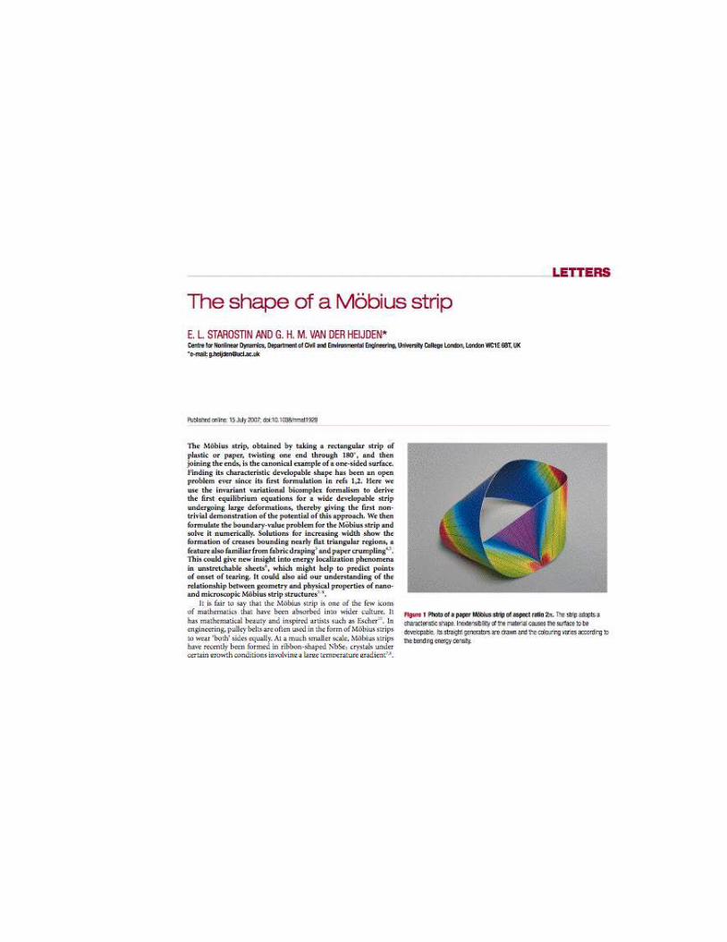
78
Invariant Variational Problems & Invariant Curve Flows Peter J. Olver University of Minnesota http://www.math.umn.edu/ ∼ olver Oxford, December, 2008
Invariant Variational Problems
&
Invariant Curve Flows
Peter J. Olver
University of Minnesota
http://www.math.umn.edu/∼ olver
Oxford, December, 2008
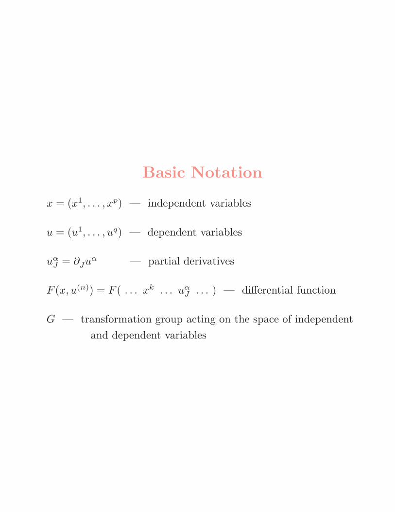
Basic Notation
x = (x1, . . . , xp) — independent variables
u = (u1, . . . , uq) — dependent variables
uαJ = ∂Juα — partial derivatives
F (x, u(n)) = F ( . . . xk . . . uαJ . . . ) — differential function
G — transformation group acting on the space of independent
and dependent variables
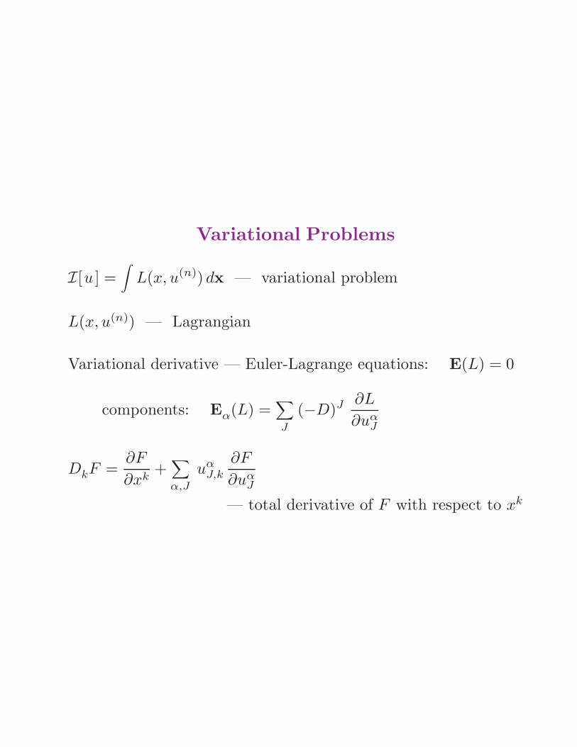
Variational Problems
I[u ] =∫
L(x, u(n)) dx — variational problem
L(x, u(n)) — Lagrangian
Variational derivative — Euler-Lagrange equations: E(L) = 0
components: Eα(L) =∑
J
(−D)J ∂L
∂uαJ
DkF =∂F
∂xk+∑
α,J
uαJ,k
∂F
∂uαJ
— total derivative of F with respect to xk
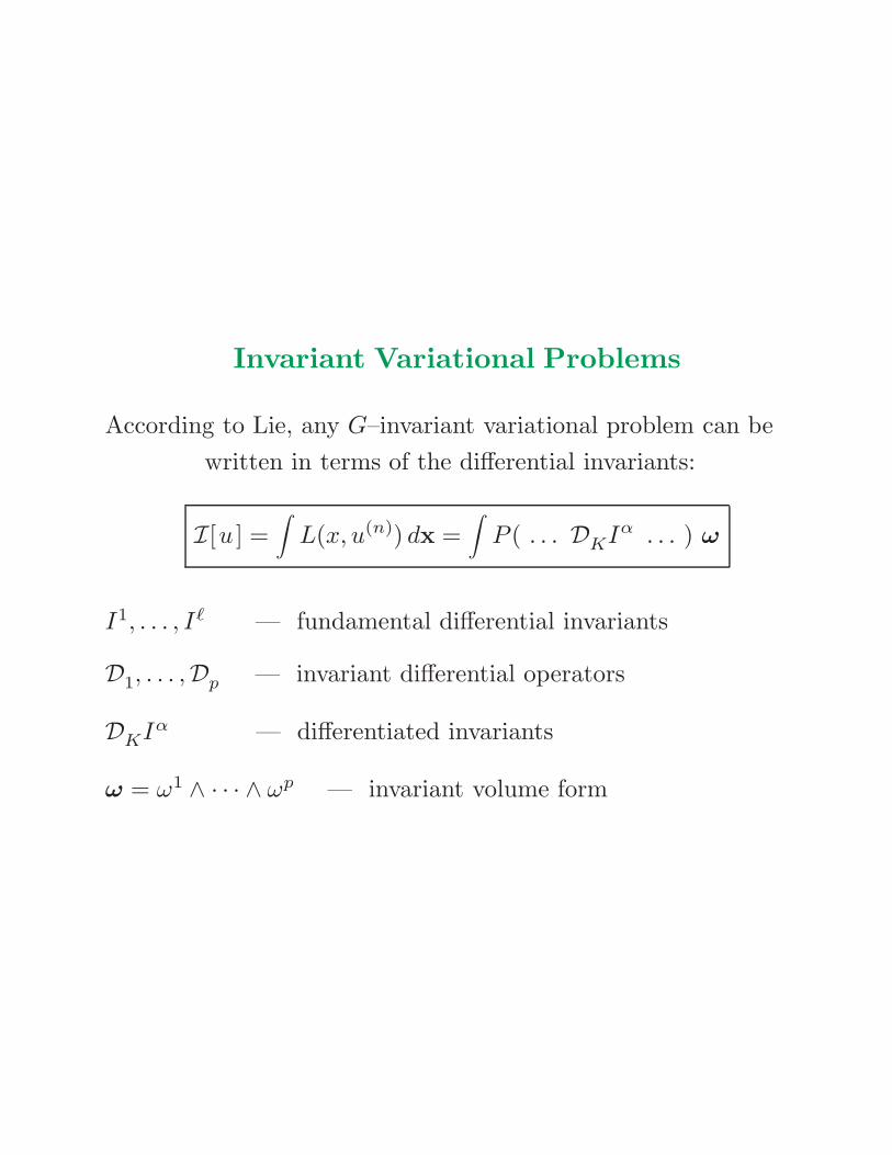
Invariant Variational Problems
According to Lie, any G–invariant variational problem can be
written in terms of the differential invariants:
I[u ] =∫
L(x, u(n)) dx =∫
P ( . . . DKIα . . . ) ω
I1, . . . , Iℓ — fundamental differential invariants
D1, . . . ,Dp — invariant differential operators
DKIα — differentiated invariants
ω = ω1 ∧ · · · ∧ ωp — invariant volume form
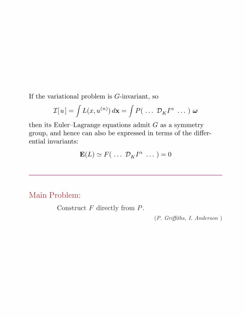
If the variational problem is G-invariant, so
I[u ] =∫
L(x, u(n)) dx =∫
P ( . . . DKIα . . . ) ω
then its Euler–Lagrange equations admit G as a symmetrygroup, and hence can also be expressed in terms of the differ-ential invariants:
E(L) ≃ F ( . . . DKIα . . . ) = 0
Main Problem:
Construct F directly from P .
(P. Griffiths, I. Anderson )
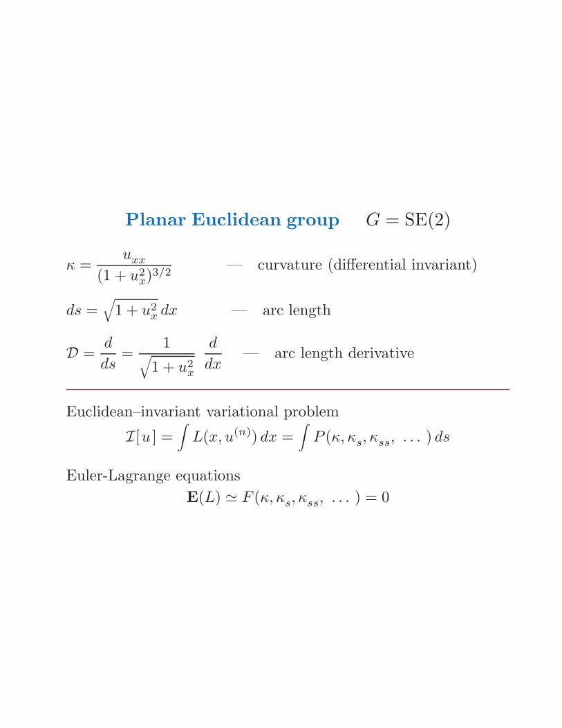
Planar Euclidean group G = SE(2)
κ =uxx
(1 + u2x)3/2
— curvature (differential invariant)
ds =√
1 + u2x dx — arc length
D =d
ds=
1√
1 + u2x
d
dx— arc length derivative
Euclidean–invariant variational problem
I[u ] =∫
L(x, u(n)) dx =∫
P (κ, κs, κss, . . . ) ds
Euler-Lagrange equations
E(L) ≃ F (κ, κs, κss, . . . ) = 0
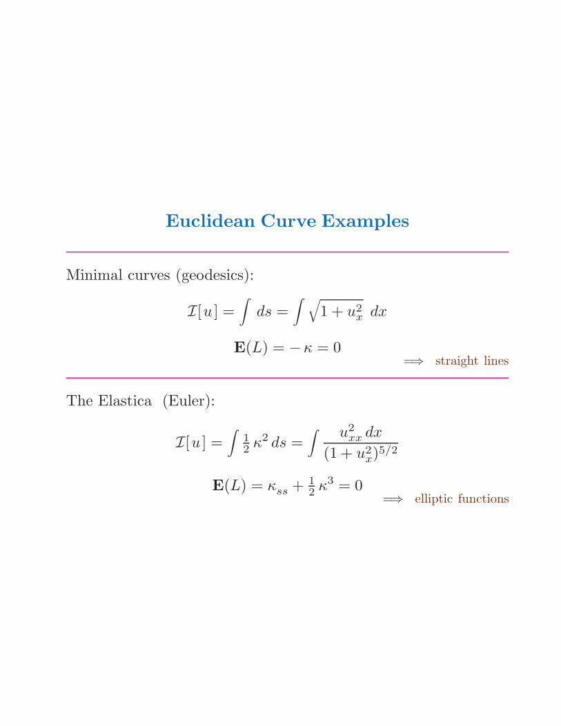
Euclidean Curve Examples
Minimal curves (geodesics):
I[u ] =∫
ds =∫ √
1 + u2x dx
E(L) = −κ = 0=⇒ straight lines
The Elastica (Euler):
I[u ] =∫
12 κ2 ds =
∫ u2xx dx
(1 + u2x)5/2
E(L) = κss + 12 κ3 = 0
=⇒ elliptic functions
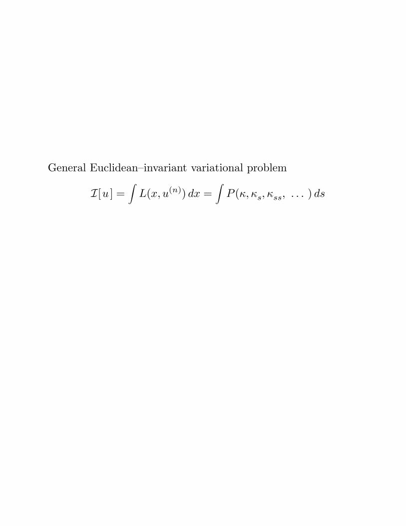
General Euclidean–invariant variational problem
I[u ] =∫
L(x, u(n)) dx =∫
P (κ, κs, κss, . . . ) ds
Invariantized Euler–Lagrange expression
E(P ) =∞∑
n=0
(−D)n ∂P
∂κn
D =d
ds
Invariantized Hamiltonian
H(P ) =∑
i>j
κi−j (−D)j ∂P
∂κi
− P
General Euclidean–invariant variational problem
I[u ] =∫
L(x, u(n)) dx =∫
P (κ, κs, κss, . . . ) ds
Invariantized Euler–Lagrange expression
E(P ) =∞∑
n=0
(−D)n ∂P
∂κn
D =d
ds
Invariantized Hamiltonian
H(P ) =∑
i>j
κi−j (−D)j ∂P
∂κi
− P
General Euclidean–invariant variational problem
I[u ] =∫
L(x, u(n)) dx =∫
P (κ, κs, κss, . . . ) ds
Invariantized Euler–Lagrange expression
E(P ) =∞∑
n=0
(−D)n ∂P
∂κn
D =d
ds
Invariantized Hamiltonian
H(P ) =∑
i>j
κi−j (−D)j ∂P
∂κi
− P
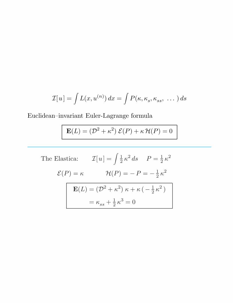
I[u ] =∫
L(x, u(n)) dx =∫
P (κ, κs, κss, . . . ) ds
Euclidean–invariant Euler-Lagrange formula
E(L) = (D2 + κ2) E(P ) + κH(P ) = 0
The Elastica: I[u ] =∫
12 κ2 ds P = 1
2 κ2
E(P ) = κ H(P ) = −P = − 12 κ2
E(L) = (D2 + κ2) κ + κ (− 12 κ2 )
= κss + 12 κ3 = 0
Applications of Moving Frames
• Differential geometry
• Equivalence
• Symmetry
• Differential invariants
• Rigidity
• Joint invariants and semi-differential invariants
• Integral invariants
• Symmetries of differential equations
• Factorization of differential operators
• Invariant differential forms and tensors
• Identities and syzygies
• Classical invariant theory
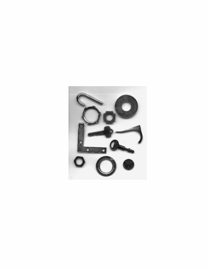
• Computer vision
object recognition
symmetry detection
structure from motion
• Invariant variational problems
• Invariant numerical methods
• Poisson geometry & solitons
• Killing tensors in relativity
• Invariants of Lie algebras in quantum mechanics
• Lie pseudo-groups
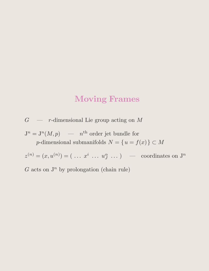
Moving Frames
G — r-dimensional Lie group acting on M
Jn = Jn(M,p) — nth order jet bundle for
p-dimensional submanifolds N = u = f(x) ⊂M
z(n) = (x, u(n)) = ( . . . xi . . . uαJ . . . ) — coordinates on Jn
G acts on Jn by prolongation (chain rule)

Definition.
An nth order moving frame is a G-equivariant map
ρ = ρ(n) : V ⊂ Jn −→ G
Equivariance:
ρ(g(n) · z(n)) =
g · ρ(z(n)) left moving frame
ρ(z(n)) · g−1 right moving frame
Note: ρleft(z(n)) = ρright(z
(n))−1
Theorem. A moving frame exists in a neighborhoodof a point z(n) ∈ Jn if and only if G acts freelyand regularly near z(n).
• free — the only group element g ∈ G which fixes one point
z ∈M is the identity: g · z = z if and only if g = e.
• locally free — the orbits have the same dimension as G.
• regular — all orbits have the same dimension and intersect
sufficiently small coordinate charts only once
( 6≈ irrational flow on the torus)
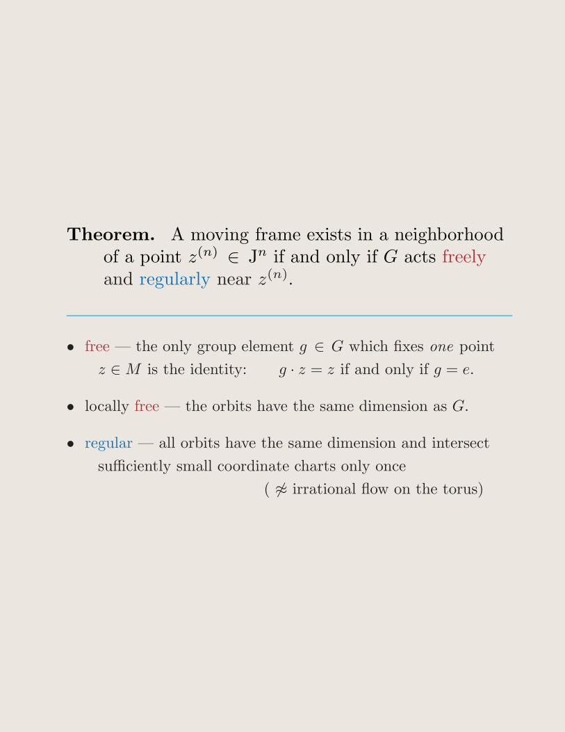
Geometric Construction
z
Oz
Normalization = choice of cross-section to the group orbits
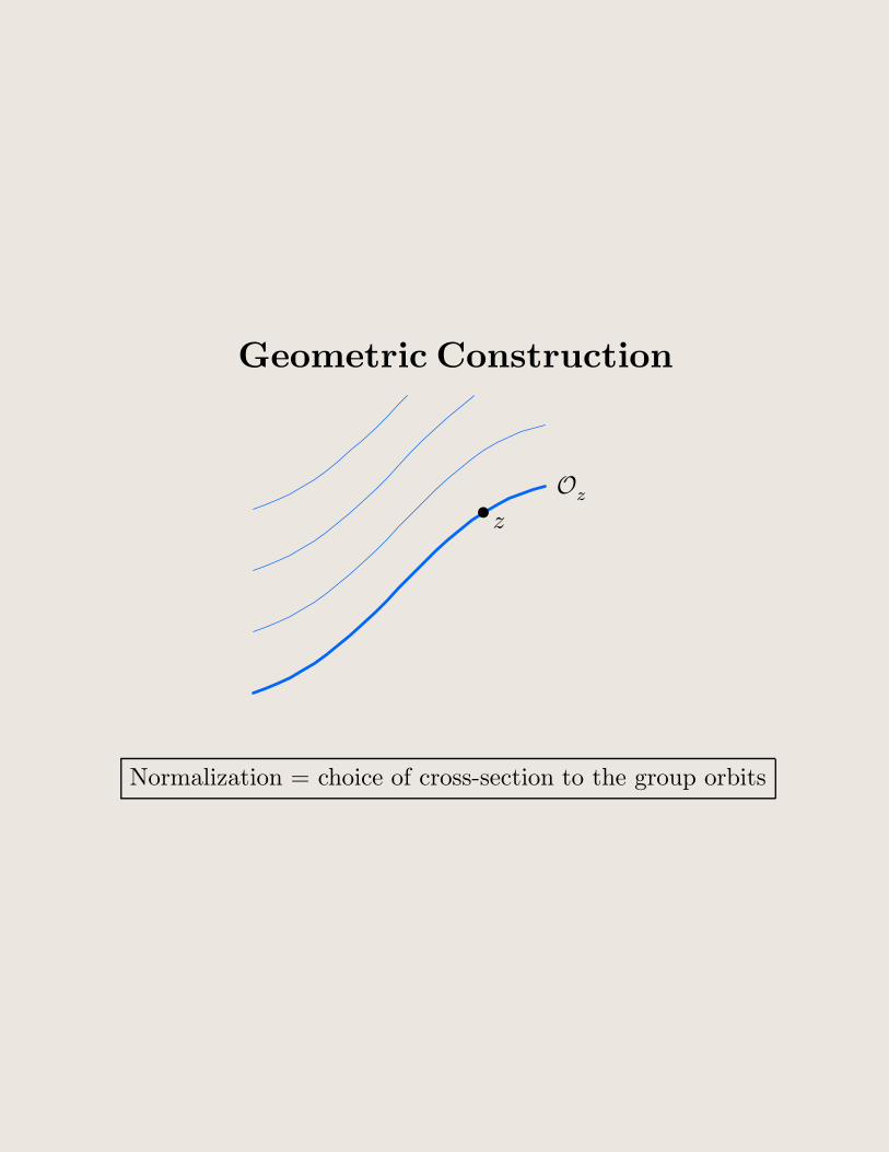
Geometric Construction
z
Oz
K
k
Normalization = choice of cross-section to the group orbits
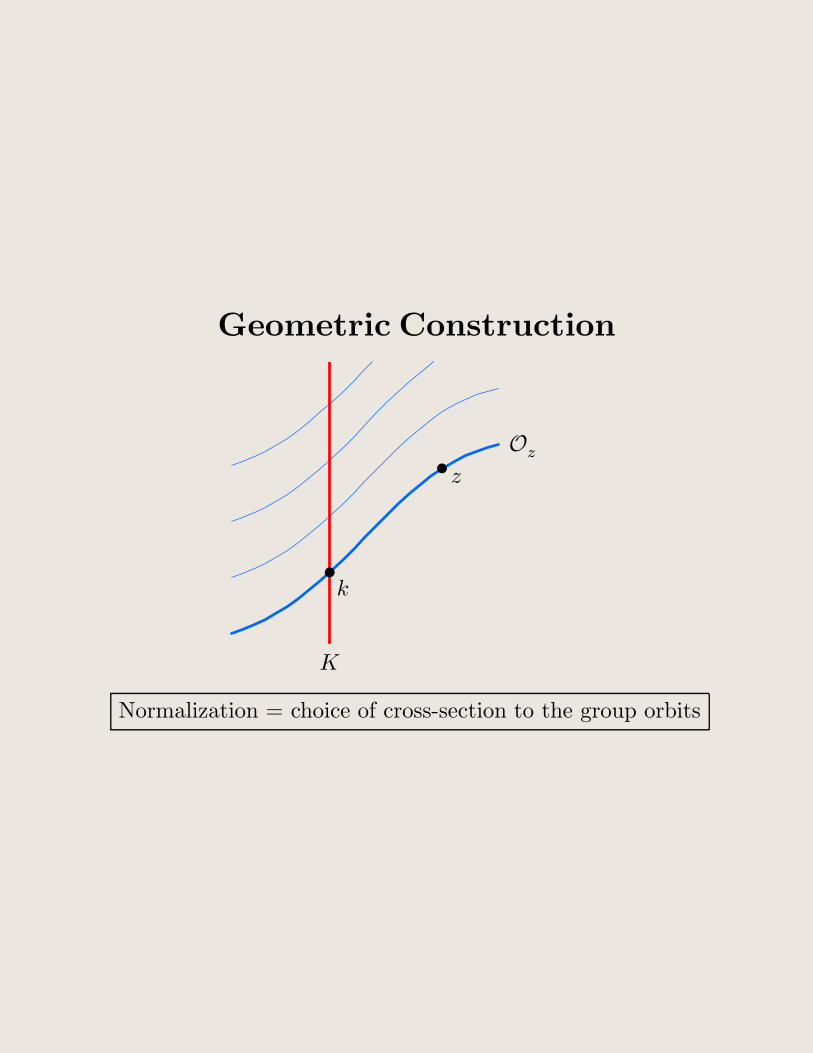
Geometric Construction
z
Oz
K
k
g = ρleft(z)
Normalization = choice of cross-section to the group orbits
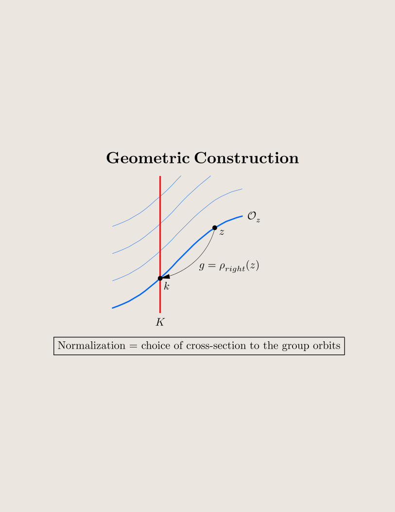
Geometric Construction
z
Oz
K
k
g = ρright(z)
Normalization = choice of cross-section to the group orbits
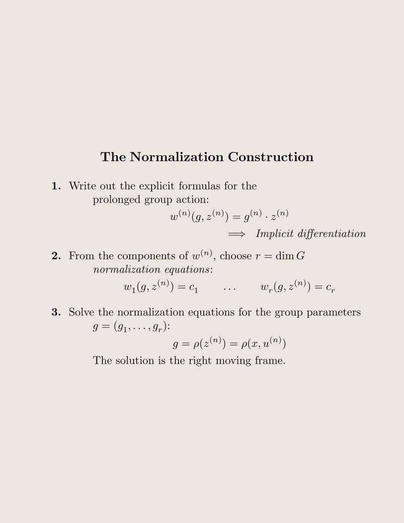
The Normalization Construction
1. Write out the explicit formulas for theprolonged group action:
w(n)(g, z(n)) = g(n) · z(n)
=⇒ Implicit differentiation
2. From the components of w(n), choose r = dim Gnormalization equations :
w1(g, z(n)) = c1 . . . wr(g, z(n)) = cr
3. Solve the normalization equations for the group parametersg = (g1, . . . , gr):
g = ρ(z(n)) = ρ(x, u(n))
The solution is the right moving frame.
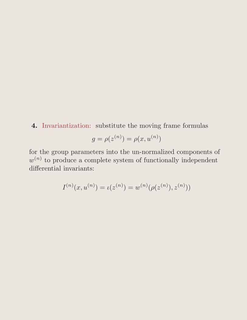
4. Invariantization: substitute the moving frame formulas
g = ρ(z(n)) = ρ(x, u(n))
for the group parameters into the un-normalized components ofw(n) to produce a complete system of functionally independentdifferential invariants:
I(n)(x, u(n)) = ι(z(n)) = w(n)(ρ(z(n)), z(n)))
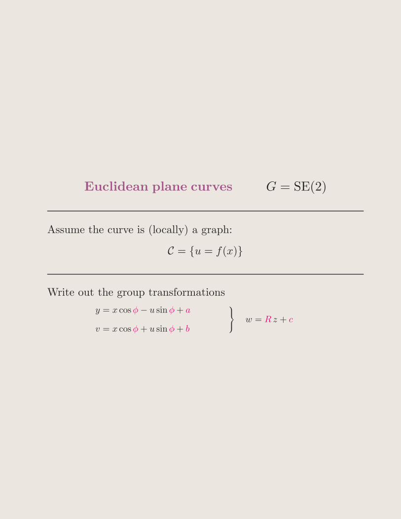
Euclidean plane curves G = SE(2)
Assume the curve is (locally) a graph:
C = u = f(x)
Write out the group transformations
y = x cosφ− u sin φ + a
v = x cosφ + u sin φ + b
w = R z + c
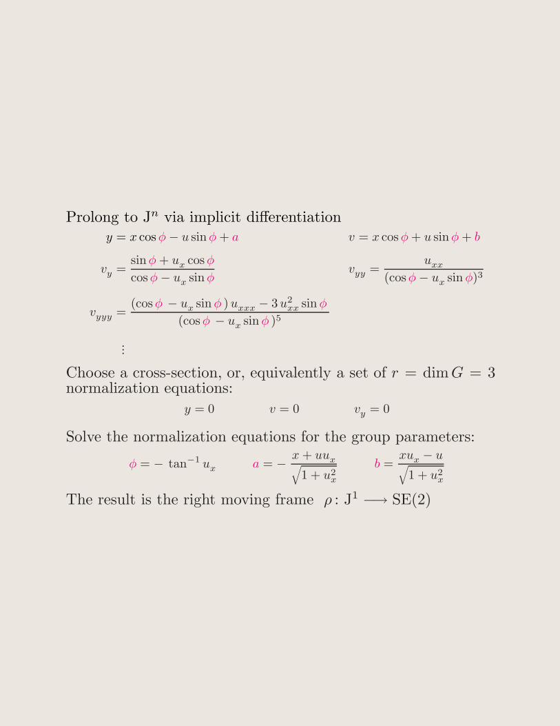
Prolong to Jn via implicit differentiationy = x cosφ− u sinφ + a v = x cosφ + u sinφ + b
vy =sinφ + ux cosφ
cosφ− ux sinφvyy =
uxx
(cosφ− ux sin φ)3
vyyy =(cosφ − ux sin φ )uxxx − 3u2
xx sin φ
(cosφ − ux sin φ )5
...
Choose a cross-section, or, equivalently a set of r = dimG = 3normalization equations:
y = 0 v = 0 vy = 0
Solve the normalization equations for the group parameters:
φ = − tan−1 ux a = −x + uux√
1 + u2x
b =xux − u√
1 + u2x
The result is the right moving frame ρ : J1 −→ SE(2)
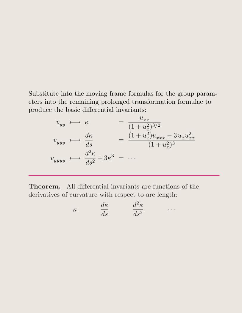
Substitute into the moving frame formulas for the group param-eters into the remaining prolonged transformation formulae toproduce the basic differential invariants:
vyy 7−→ κ =uxx
(1 + u2x)3/2
vyyy 7−→dκ
ds=
(1 + u2x)uxxx − 3uxu2
xx
(1 + u2x)3
vyyyy 7−→d2κ
ds2+ 3κ3 = · · ·
Theorem. All differential invariants are functions of thederivatives of curvature with respect to arc length:
κdκ
ds
d2κ
ds2· · ·
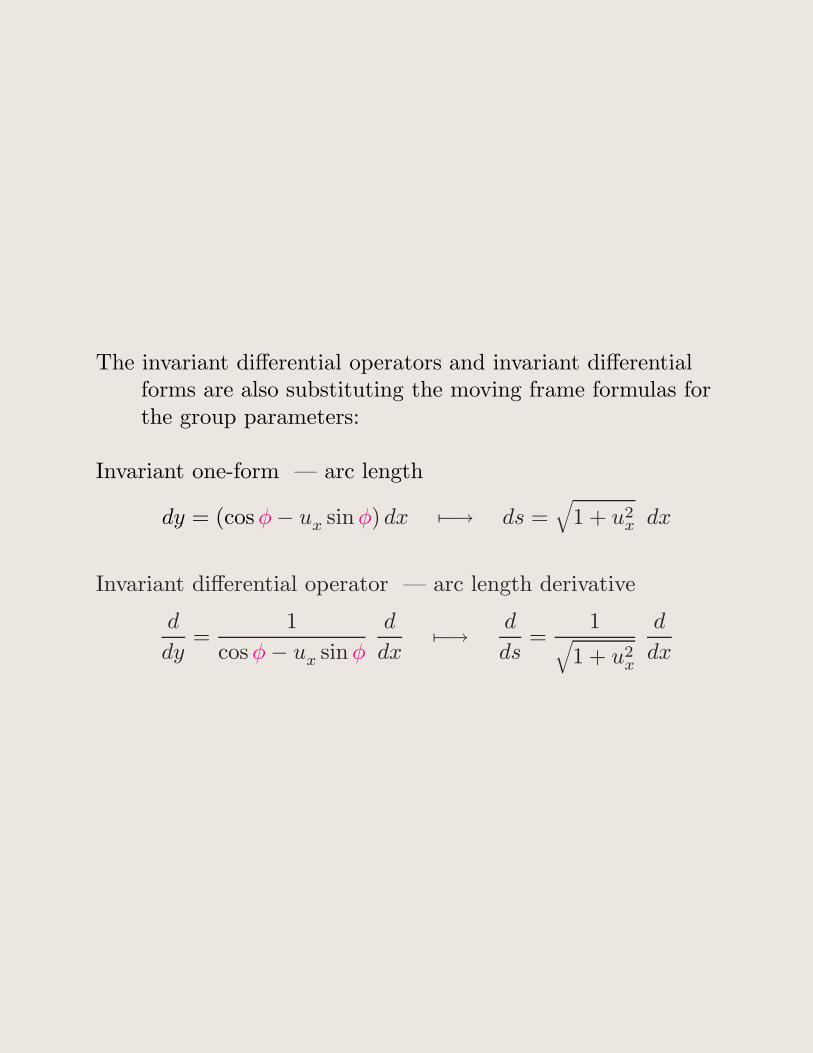
The invariant differential operators and invariant differentialforms are also substituting the moving frame formulas forthe group parameters:
Invariant one-form — arc length
dy = (cosφ− ux sin φ) dx 7−→ ds =√
1 + u2x dx
Invariant differential operator — arc length derivative
d
dy=
1
cosφ− ux sin φ
d
dx7−→
d
ds=
1√
1 + u2x
d
dx
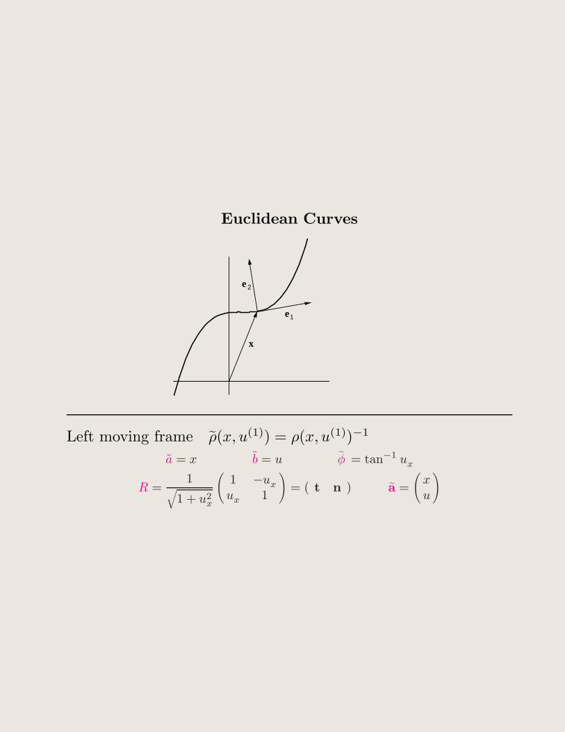
Euclidean Curves
x
e1
e 2
Left moving frame ρ(x, u(1)) = ρ(x, u(1))−1
a = x b = u φ = tan−1 ux
R =1
√1 + u2
x
(1 −ux
ux 1
)= ( t n ) a =
(xu
)
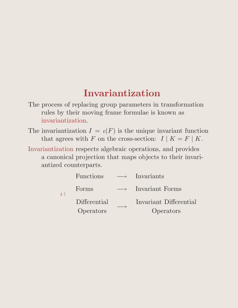
InvariantizationThe process of replacing group parameters in transformation
rules by their moving frame formulae is known asinvariantization.
The invariantization I = ι(F ) is the unique invariant functionthat agrees with F on the cross-section: I | K = F | K.
Invariantization respects algebraic operations, and providesa canonical projection that maps objects to their invari-antized counterparts.
ι :
Functions −→ Invariants
Forms −→ Invariant Forms
Differential
Operators−→
Invariant Differential
Operators
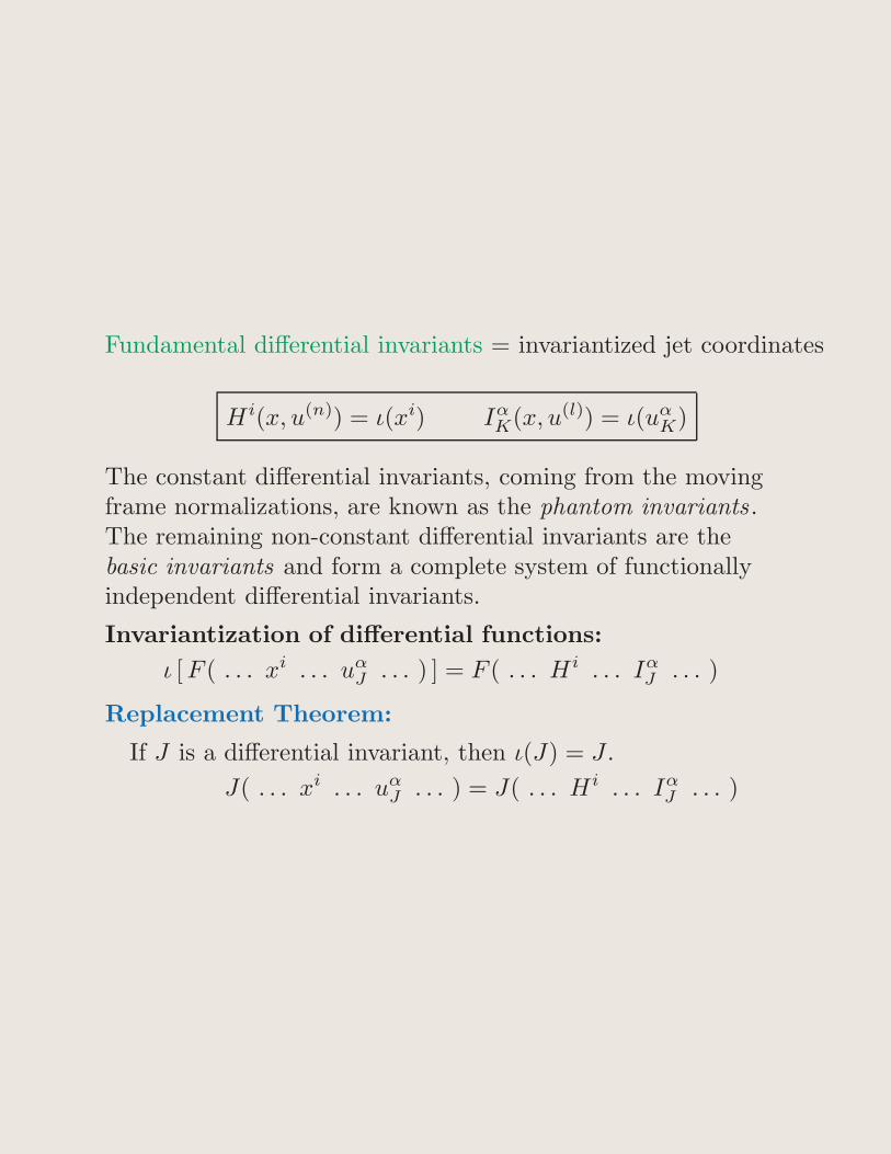
Fundamental differential invariants = invariantized jet coordinates
Hi(x, u(n)) = ι(xi) IαK(x, u(l)) = ι(uα
K)
The constant differential invariants, coming from the movingframe normalizations, are known as the phantom invariants .The remaining non-constant differential invariants are thebasic invariants and form a complete system of functionallyindependent differential invariants.
Invariantization of differential functions:
ι [ F ( . . . xi . . . uαJ . . . ) ] = F ( . . . Hi . . . Iα
J . . . )
Replacement Theorem:
If J is a differential invariant, then ι(J) = J .
J( . . . xi . . . uαJ . . . ) = J( . . . Hi . . . Iα
J . . . )
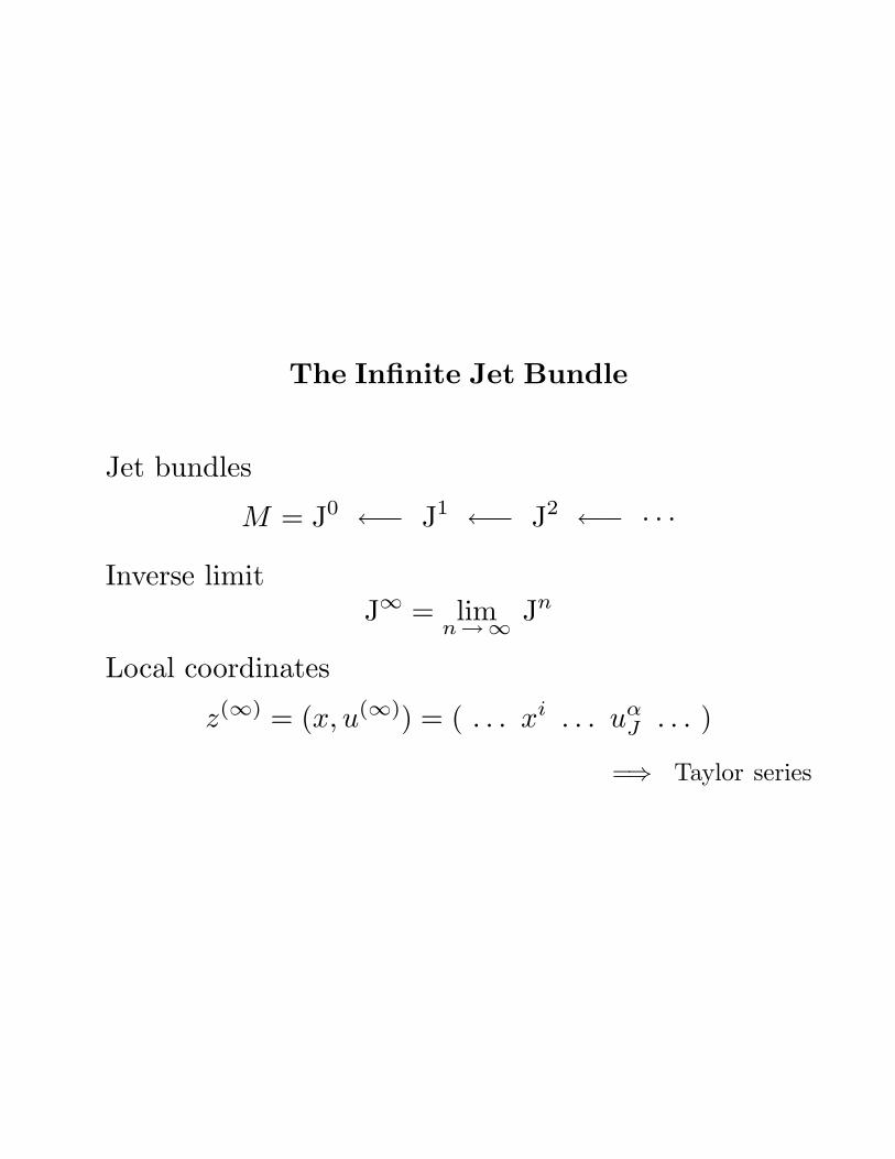
The Infinite Jet Bundle
Jet bundles
M = J0 ←− J1 ←− J2 ←− · · ·
Inverse limitJ∞ = lim
n→∞Jn
Local coordinates
z(∞) = (x, u(∞)) = ( . . . xi . . . uαJ . . . )
=⇒ Taylor series
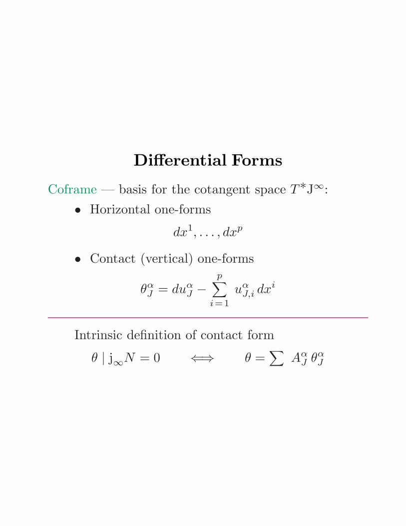
Differential Forms
Coframe — basis for the cotangent space T∗J∞:
• Horizontal one-forms
dx1, . . . , dxp
• Contact (vertical) one-forms
θαJ = duα
J −p∑
i=1
uαJ,i dxi
Intrinsic definition of contact form
θ | j∞
N = 0 ⇐⇒ θ =∑
AαJ θα
J
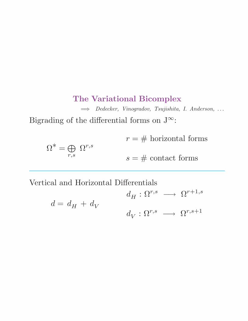
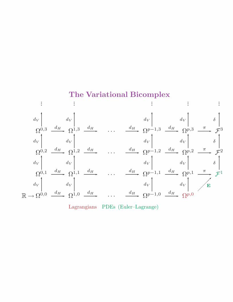
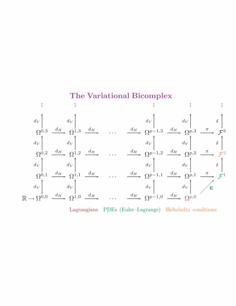
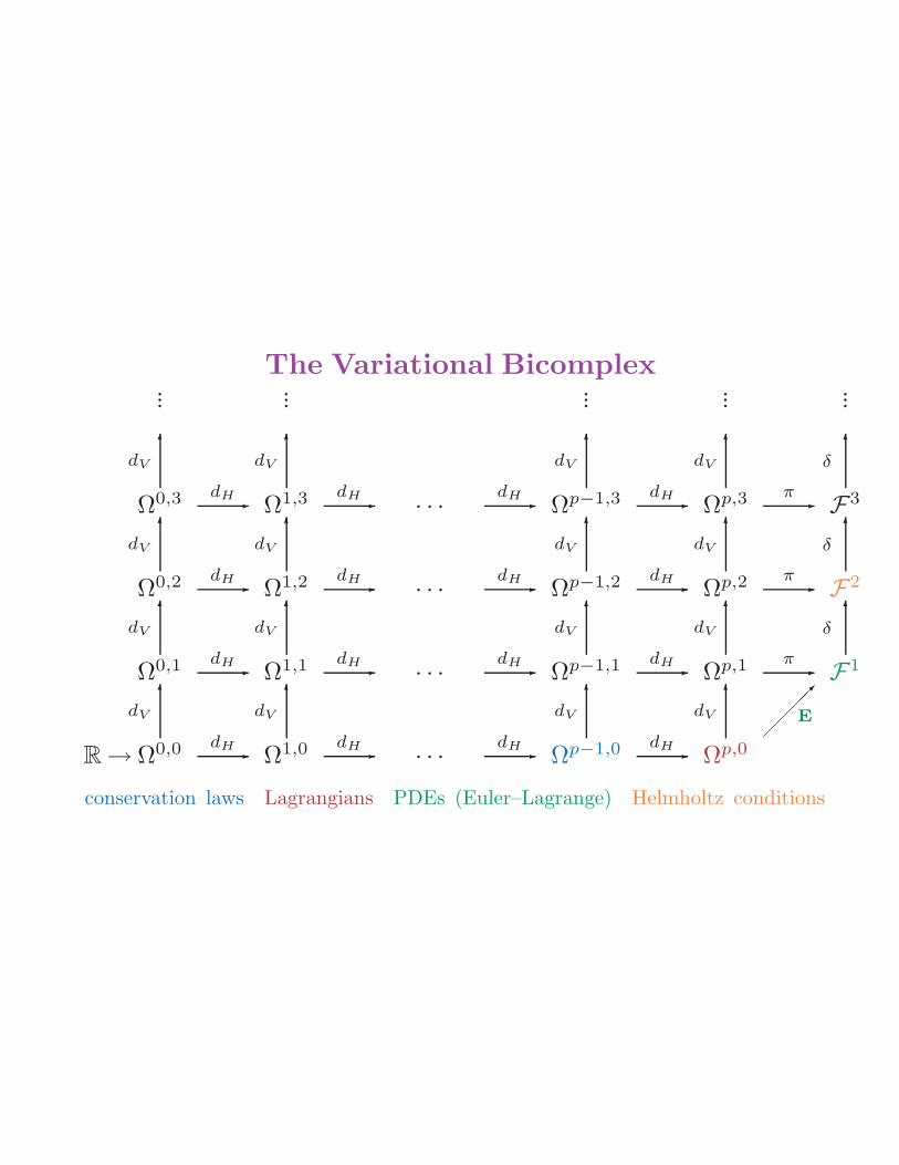
The Variational Bicomplex
=⇒ Dedecker, Vinogradov, Tsujishita, I. Anderson, . . .
Bigrading of the differential forms on J∞:
Ω∗ =M
r,sΩr,s
r = # horizontal forms
s = # contact forms
Vertical and Horizontal Differentials
d = dH + dV
dH : Ωr,s −→ Ωr+1,s
dV : Ωr,s −→ Ωr,s+1
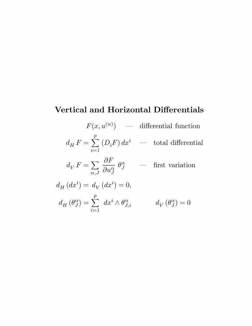
Vertical and Horizontal Differentials
F (x, u(n)) — differential function
dH F =p∑
i=1
(DiF ) dxi — total differential
dV F =∑
α,J
∂F
∂uαJ
θαJ — first variation
dH (dxi) = dV (dxi) = 0,
dH (θαJ ) =
p∑
i=1
dxi ∧ θαJ,i dV (θα
J ) = 0
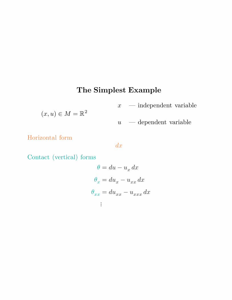
The Simplest Example
(x, u) ∈M = R2
x — independent variable
u — dependent variable
Horizontal formdx
Contact (vertical) forms
θ = du− ux dx
θx = dux − uxx dx
θxx = duxx − uxxx dx
...
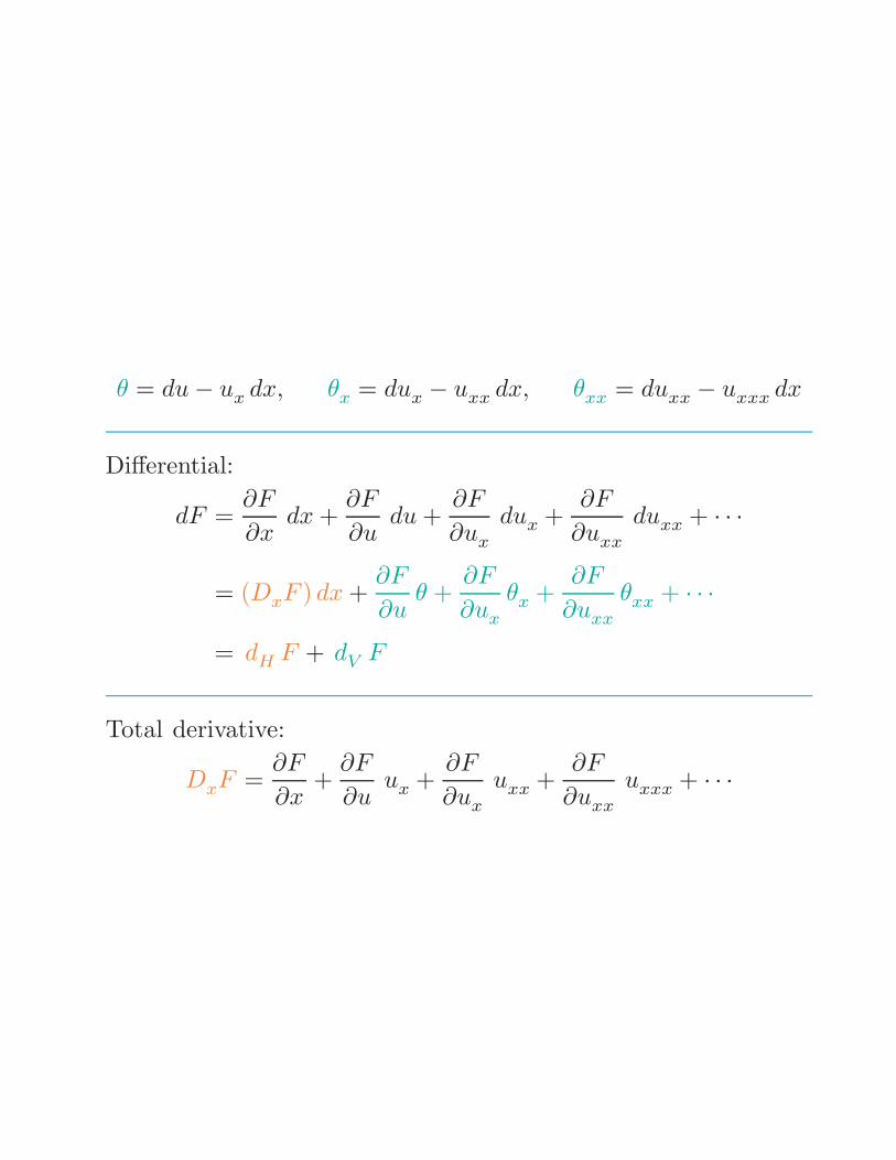
θ = du− ux dx, θx = dux − uxx dx, θxx = duxx − uxxx dx
Differential:
dF =∂F
∂xdx +
∂F
∂udu +
∂F
∂ux
dux +∂F
∂uxx
duxx + · · ·
= (DxF ) dx +∂F
∂uθ +
∂F
∂ux
θx +∂F
∂uxx
θxx + · · ·
= dH F + dV F
Total derivative:
DxF =∂F
∂x+
∂F
∂uux +
∂F
∂ux
uxx +∂F
∂uxx
uxxx + · · ·
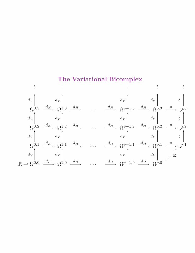
The Variational Bicomplex... ... ... ... ...
dV
6dV
6dV
6dV
6δ
6
Ω0,3 dH- Ω1,3 dH- · · ·dH- Ωp−1,3 dH- Ωp,3 π
- F3
dV
6dV
6dV
6dV
6δ
6
Ω0,2 dH- Ω1,2 dH- · · ·dH- Ωp−1,2 dH- Ωp,2 π
- F2
dV
6dV
6dV
6dV
6δ
6
Ω0,1 dH- Ω1,1 dH- · · ·dH- Ωp−1,1 dH- Ωp,1 π
- F1
dV
6dV
6dV
6dV
6
E
R→ Ω0,0 dH- Ω1,0 dH- · · ·dH- Ωp−1,0 dH- Ωp,0
conservation laws Lagrangians PDEs (Euler–Lagrange) Helmholtz conditions
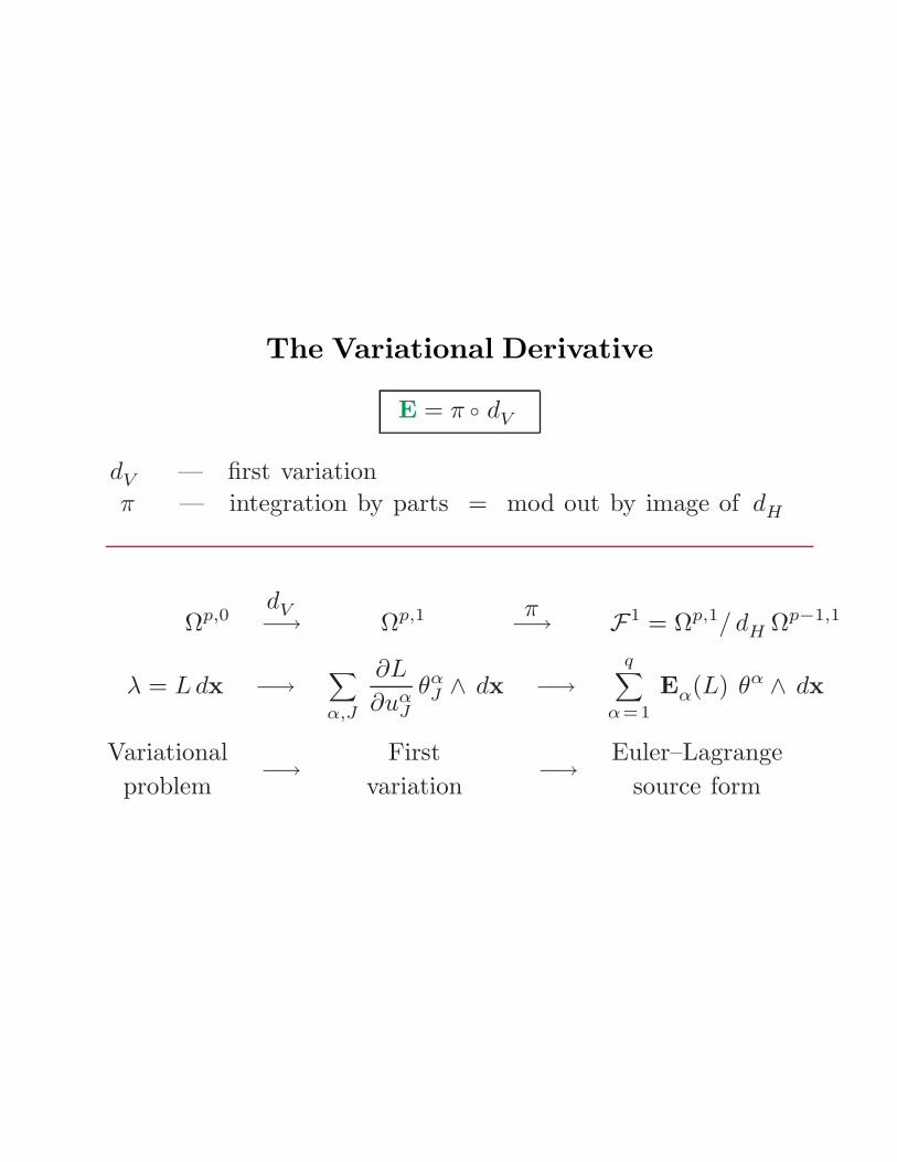
The Variational Derivative
E = π dV
dV — first variation
π — integration by parts = mod out by image of dH
Ωp,0 −→dV
Ωp,1 −→π
F1 = Ωp,1/ dH Ωp−1,1
λ = Ldx −→∑
α,J
∂L
∂uαJ
θαJ ∧ dx −→
q∑
α=1
Eα(L) θα ∧ dx
Variational
problem−→
First
variation−→
Euler–Lagrange
source form
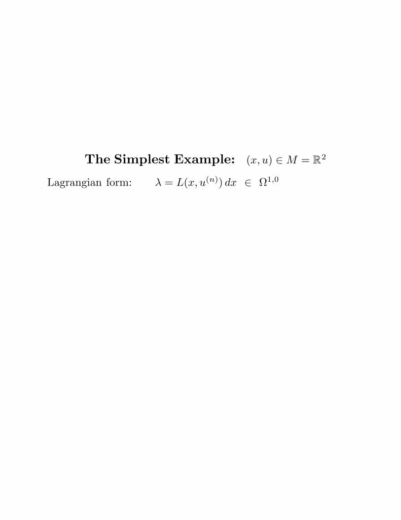
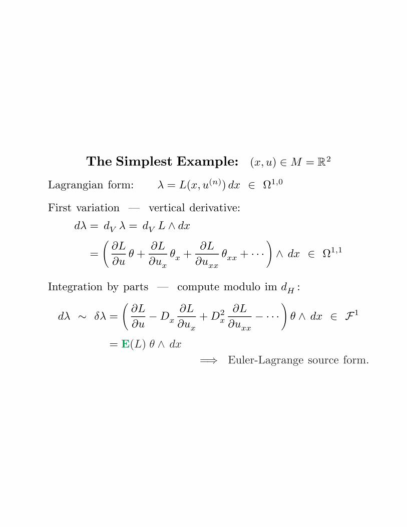
The Simplest Example: (x, u) ∈M = R2
Lagrangian form: λ = L(x, u(n)) dx ∈ Ω1,0
First variation — vertical derivative:
dλ = dV λ = dV L ∧ dx
=
(∂L
∂uθ +
∂L
∂ux
θx +∂L
∂uxx
θxx + · · ·
)∧ dx ∈ Ω1,1
Integration by parts — compute modulo im dH :
dλ ∼ δλ =
(∂L
∂u−Dx
∂L
∂ux
+ D2x
∂L
∂uxx
− · · ·
)θ ∧ dx ∈ F1
= E(L) θ ∧ dx
=⇒ Euler-Lagrange source form.
To analyze invariant variational prob-
lems, invariant conservation laws, etc., we
apply the moving frame invariantization
process to the variational bicomplex:
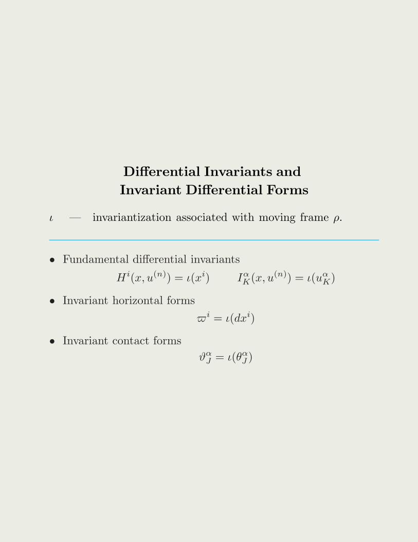
Differential Invariants and
Invariant Differential Forms
ι — invariantization associated with moving frame ρ.
• Fundamental differential invariants
Hi(x, u(n)) = ι(xi) IαK(x, u(n)) = ι(uα
K)
• Invariant horizontal forms
i = ι(dxi)
• Invariant contact forms
ϑαJ = ι(θα
J )
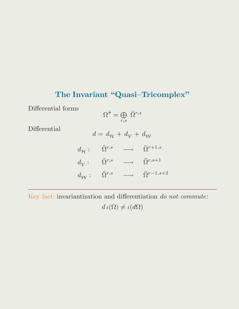
The Invariant “Quasi–Tricomplex”
Differential formsΩ∗ =
M
r,sΩr,s
Differentiald = d
H+ d
V+ d
W
dH
: Ωr,s −→ Ωr+1,s
dV
: Ωr,s −→ Ωr,s+1
dW
: Ωr,s −→ Ωr−1,s+2
Key fact: invariantization and differentiation do not commute:
d ι(Ω) 6= ι(dΩ)
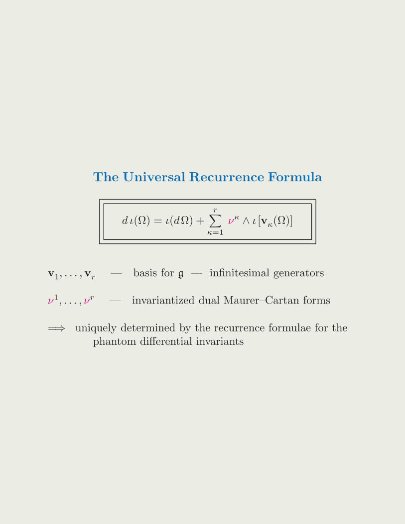
The Universal Recurrence Formula
d ι(Ω) = ι(dΩ) +r∑
κ=1
νκ ∧ ι [vκ(Ω)]
v1, . . . ,vr — basis for g — infinitesimal generators
ν1, . . . , νr — invariantized dual Maurer–Cartan forms
=⇒ uniquely determined by the recurrence formulae for thephantom differential invariants
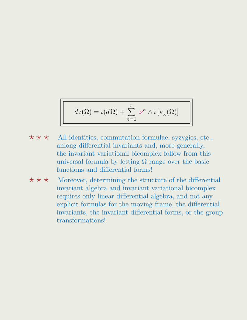
d ι(Ω) = ι(dΩ) +r∑
κ=1
νκ ∧ ι [vκ(Ω)]
⋆ ⋆ ⋆ All identities, commutation formulae, syzygies, etc.,among differential invariants and, more generally,the invariant variational bicomplex follow from thisuniversal formula by letting Ω range over the basicfunctions and differential forms!
⋆ ⋆ ⋆ Moreover, determining the structure of the differentialinvariant algebra and invariant variational bicomplexrequires only linear differential algebra, and not anyexplicit formulas for the moving frame, the differentialinvariants, the invariant differential forms, or the grouptransformations!
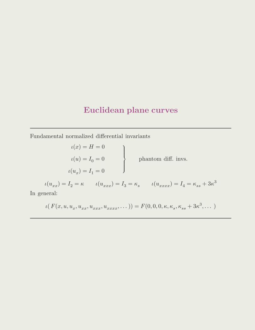
Euclidean plane curves
Fundamental normalized differential invariants
ι(x) = H = 0
ι(u) = I0 = 0
ι(ux) = I1 = 0
phantom diff. invs.
ι(uxx) = I2 = κ ι(uxxx) = I3 = κs ι(uxxxx) = I4 = κss + 3κ3
In general:
ι( F (x, u, ux, uxx, uxxx, uxxxx, . . . )) = F (0, 0, 0, κ, κs, κss + 3κ3, . . . )
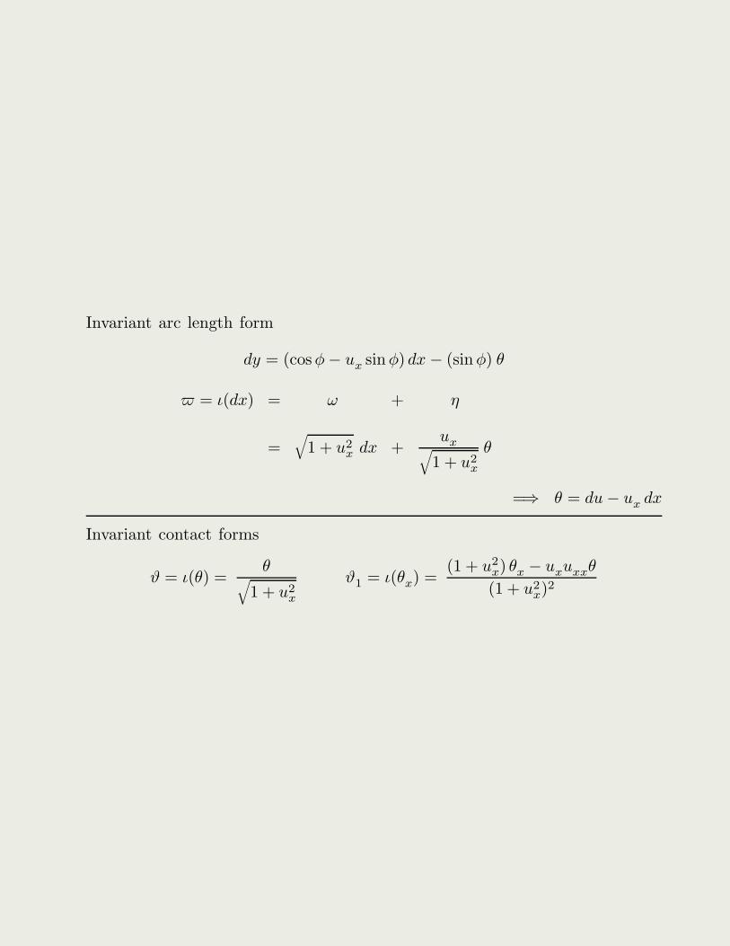
Invariant arc length form
dy = (cosφ− ux sin φ) dx − (sin φ) θ
= ι(dx) = ω + η
=√
1 + u2x dx +
ux√1 + u2
x
θ
=⇒ θ = du− ux dx
Invariant contact forms
ϑ = ι(θ) =θ
√1 + u2
x
ϑ1 = ι(θx) =(1 + u2
x) θx − uxuxxθ
(1 + u2x)2
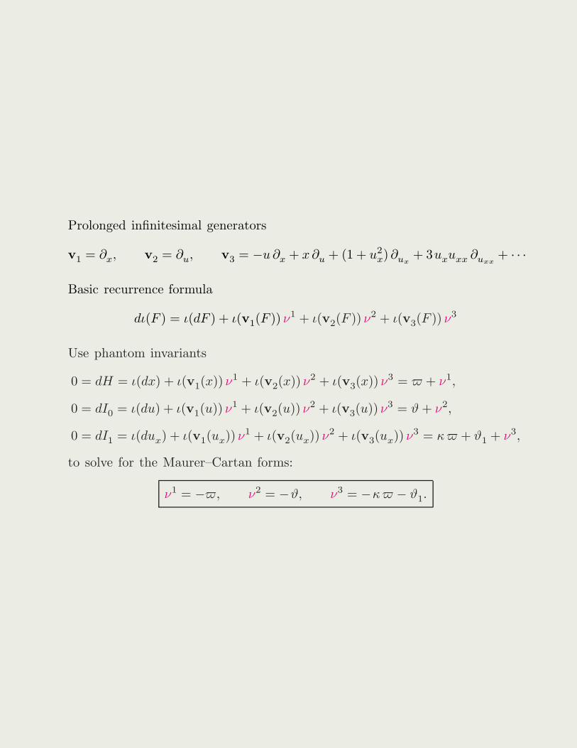
Prolonged infinitesimal generators
v1 = ∂x, v2 = ∂u, v3 = −u ∂x + x∂u + (1 + u2x) ∂ux
+ 3uxuxx ∂uxx+ · · ·
Basic recurrence formula
dι(F ) = ι(dF ) + ι(v1(F )) ν1 + ι(v2(F )) ν2 + ι(v3(F )) ν3
Use phantom invariants
0 = dH = ι(dx) + ι(v1(x)) ν1 + ι(v2(x)) ν2 + ι(v3(x)) ν3 = + ν1,
0 = dI0 = ι(du) + ι(v1(u)) ν1 + ι(v2(u)) ν2 + ι(v3(u)) ν3 = ϑ + ν2,
0 = dI1 = ι(dux) + ι(v1(ux)) ν1 + ι(v2(ux)) ν2 + ι(v3(ux)) ν3 = κ + ϑ1 + ν3,
to solve for the Maurer–Cartan forms:
ν1 = −, ν2 = −ϑ, ν3 = −κ − ϑ1.
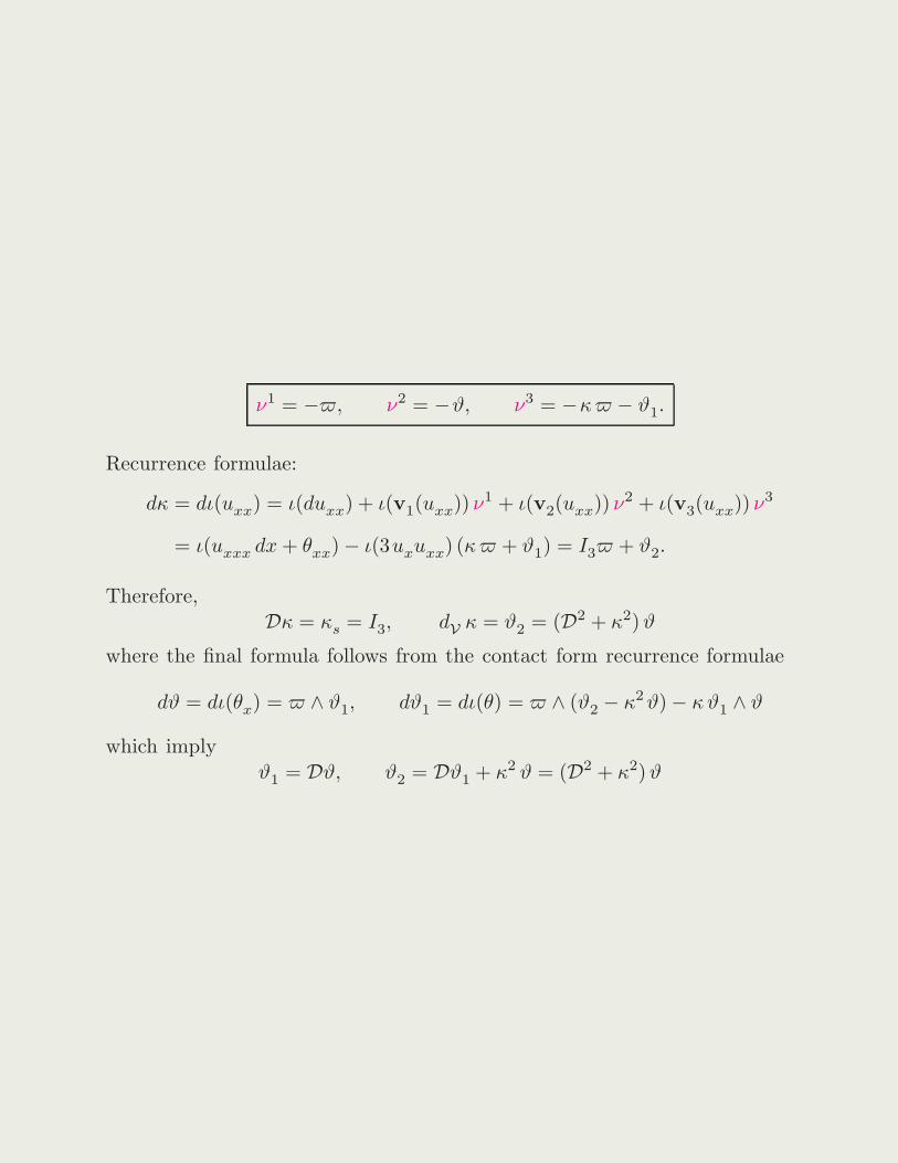
ν1 = −, ν2 = −ϑ, ν3 = −κ − ϑ1.
Recurrence formulae:
dκ = dι(uxx) = ι(duxx) + ι(v1(uxx)) ν1 + ι(v2(uxx)) ν2 + ι(v3(uxx)) ν3
= ι(uxxx dx + θxx)− ι(3uxuxx) (κ + ϑ1) = I3 + ϑ2.
Therefore,Dκ = κs = I3, d
Vκ = ϑ2 = (D2 + κ2)ϑ
where the final formula follows from the contact form recurrence formulae
dϑ = dι(θx) = ∧ ϑ1, dϑ1 = dι(θ) = ∧ (ϑ2 − κ2 ϑ)− κϑ1 ∧ ϑ
which imply
ϑ1 = Dϑ, ϑ2 = Dϑ1 + κ2 ϑ = (D2 + κ2)ϑ
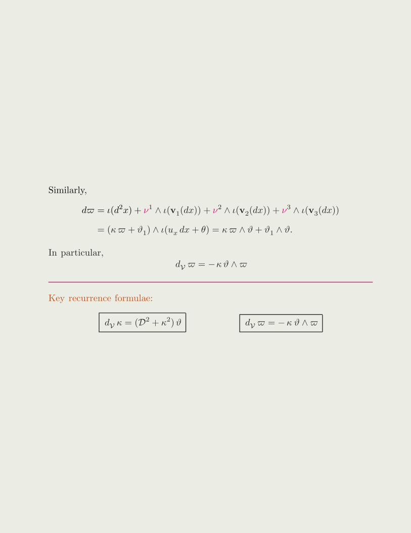
Similarly,
d = ι(d2x) + ν1 ∧ ι(v1(dx)) + ν2 ∧ ι(v2(dx)) + ν3 ∧ ι(v3(dx))
= (κ + ϑ1) ∧ ι(ux dx + θ) = κ ∧ ϑ + ϑ1 ∧ ϑ.
In particular,dV
= −κϑ ∧
Key recurrence formulae:
dV
κ = (D2 + κ2)ϑ dV
= −κ ϑ ∧
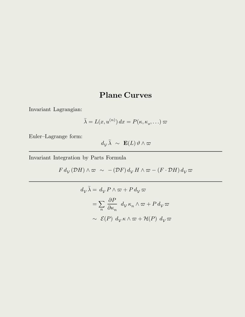
Plane Curves
Invariant Lagrangian:
λ = L(x, u(n)) dx = P (κ, κs, . . .)
Euler–Lagrange form:dV
λ ∼ E(L)ϑ ∧
Invariant Integration by Parts Formula
F dV
(DH) ∧ ∼ − (DF ) dV
H ∧ − (F · DH) dV
dV
λ = dV
P ∧ + P dV
=∑
n
∂P
∂κn
dV
κn ∧ + P dV
∼ E(P ) dV
κ ∧ +H(P ) dV
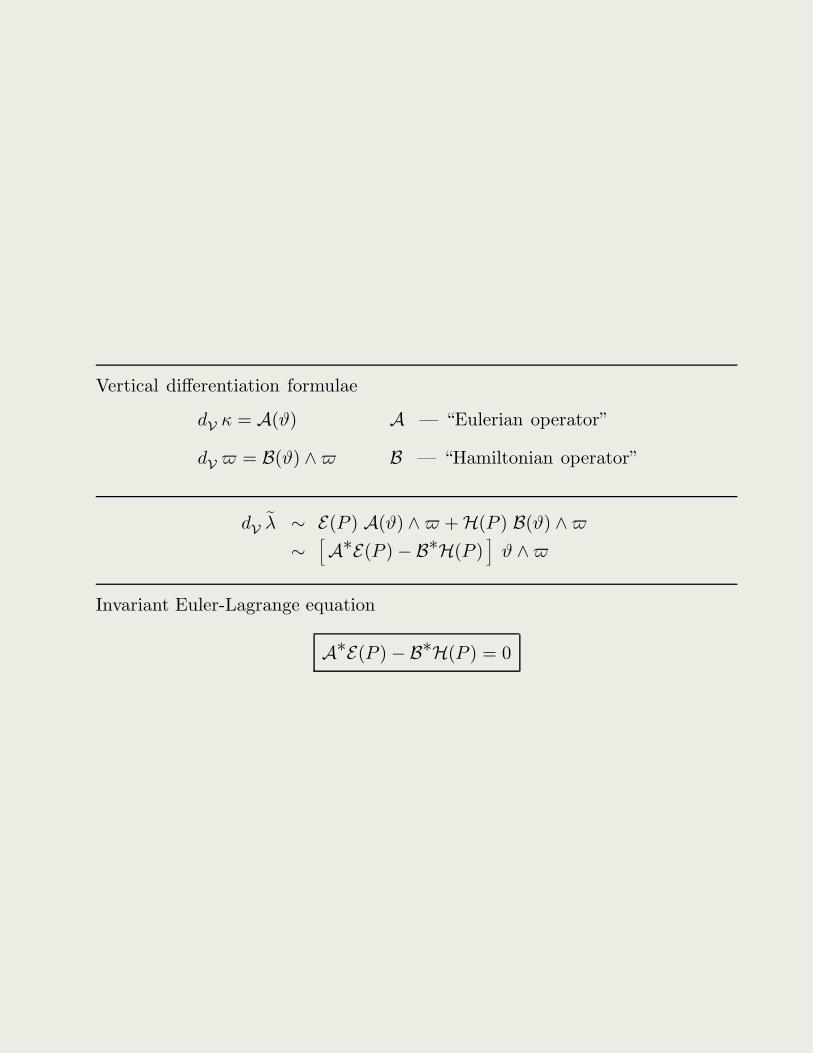
Vertical differentiation formulae
dV
κ = A(ϑ) A — “Eulerian operator”
dV
= B(ϑ) ∧ B — “Hamiltonian operator”
dV
λ ∼ E(P ) A(ϑ) ∧ +H(P ) B(ϑ) ∧
∼[A∗E(P )− B∗H(P )
]ϑ ∧
Invariant Euler-Lagrange equation
A∗E(P )− B∗H(P ) = 0
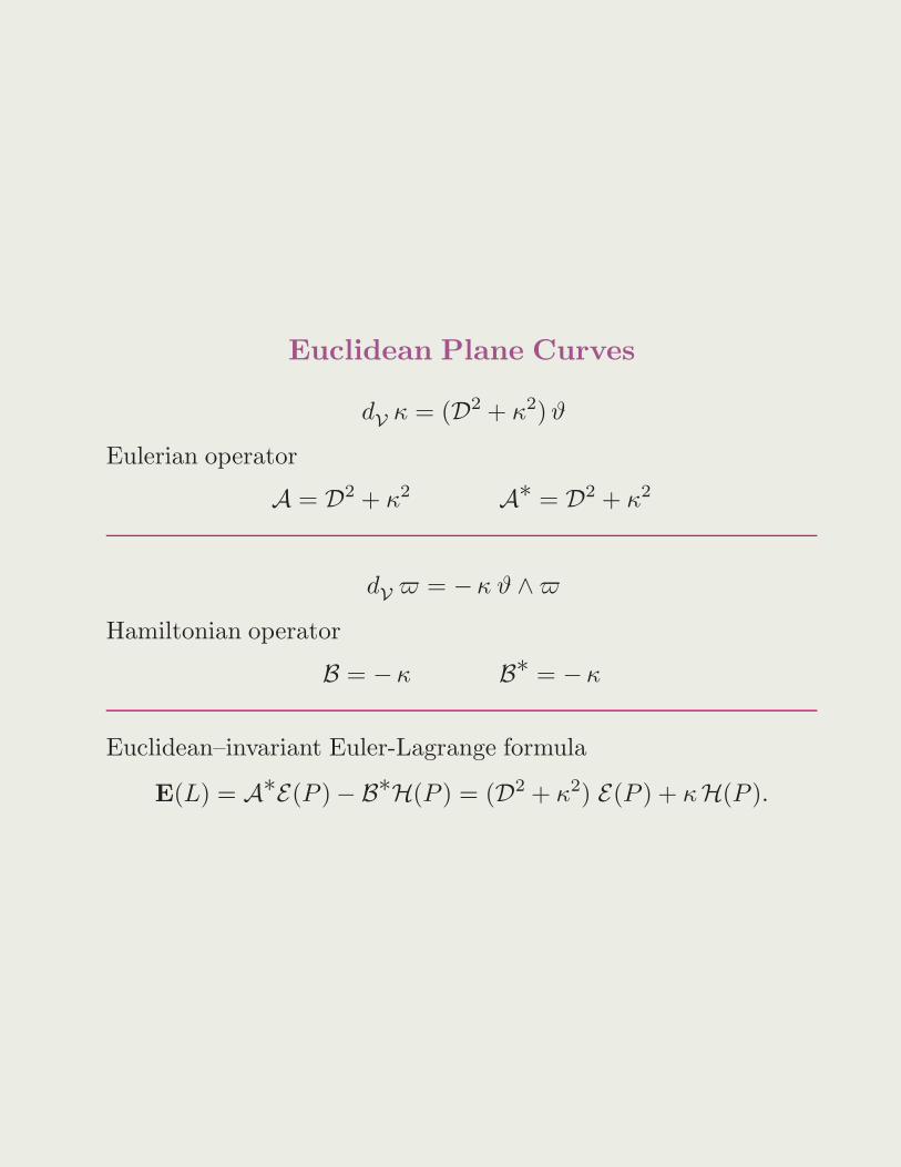
Euclidean Plane Curves
dV
κ = (D2 + κ2)ϑ
Eulerian operator
A = D2 + κ2 A∗ = D2 + κ2
dV
= −κ ϑ ∧
Hamiltonian operator
B = −κ B∗ = −κ
Euclidean–invariant Euler-Lagrange formula
E(L) = A∗E(P )− B∗H(P ) = (D2 + κ2) E(P ) + κH(P ).
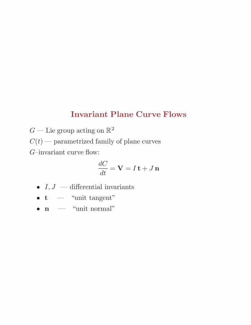
Invariant Plane Curve Flows
G — Lie group acting on R2
C(t) — parametrized family of plane curves
G–invariant curve flow:
dC
dt= V = I t + J n
• I, J — differential invariants
• t — “unit tangent”
• n — “unit normal”
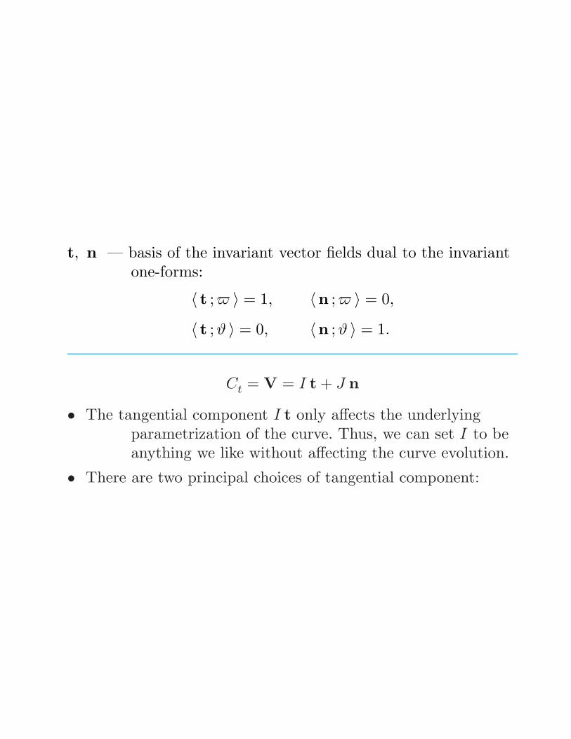
t, n — basis of the invariant vector fields dual to the invariantone-forms:
〈 t ; 〉 = 1, 〈n ; 〉 = 0,
〈 t ;ϑ 〉 = 0, 〈n ;ϑ 〉 = 1.
Ct = V = I t + J n
• The tangential component I t only affects the underlyingparametrization of the curve. Thus, we can set I to beanything we like without affecting the curve evolution.
• There are two principal choices of tangential component:
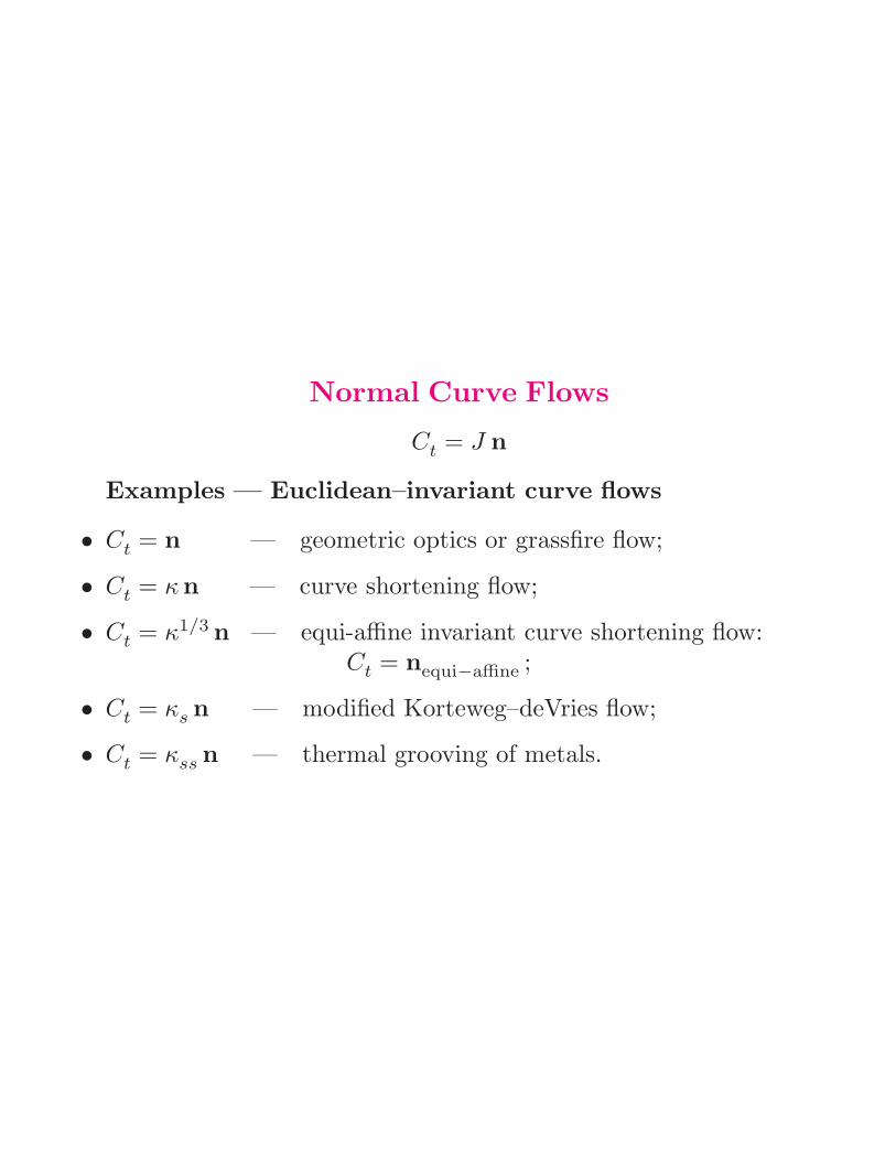
Normal Curve Flows
Ct = J n
Examples — Euclidean–invariant curve flows
• Ct = n — geometric optics or grassfire flow;
• Ct = κn — curve shortening flow;
• Ct = κ1/3 n — equi-affine invariant curve shortening flow:Ct = nequi−affine ;
• Ct = κs n — modified Korteweg–deVries flow;
• Ct = κss n — thermal grooving of metals.
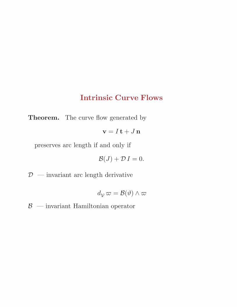
Intrinsic Curve Flows
Theorem. The curve flow generated by
v = I t + J n
preserves arc length if and only if
B(J) +D I = 0.
D — invariant arc length derivative
dV
= B(ϑ) ∧
B — invariant Hamiltonian operator
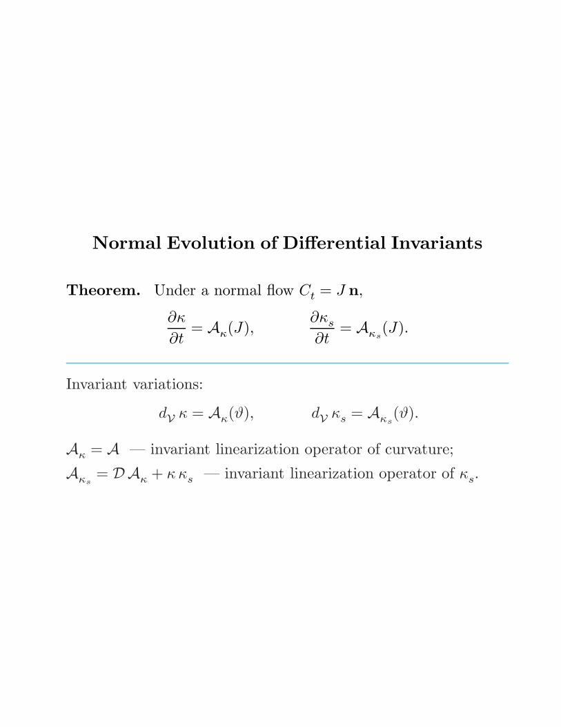
Normal Evolution of Differential Invariants
Theorem. Under a normal flow Ct = J n,
∂κ
∂t= Aκ(J),
∂κs
∂t= Aκs
(J).
Invariant variations:
dV
κ = Aκ(ϑ), dV
κs = Aκs(ϑ).
Aκ = A — invariant linearization operator of curvature;
Aκs= DAκ + κ κs — invariant linearization operator of κs.
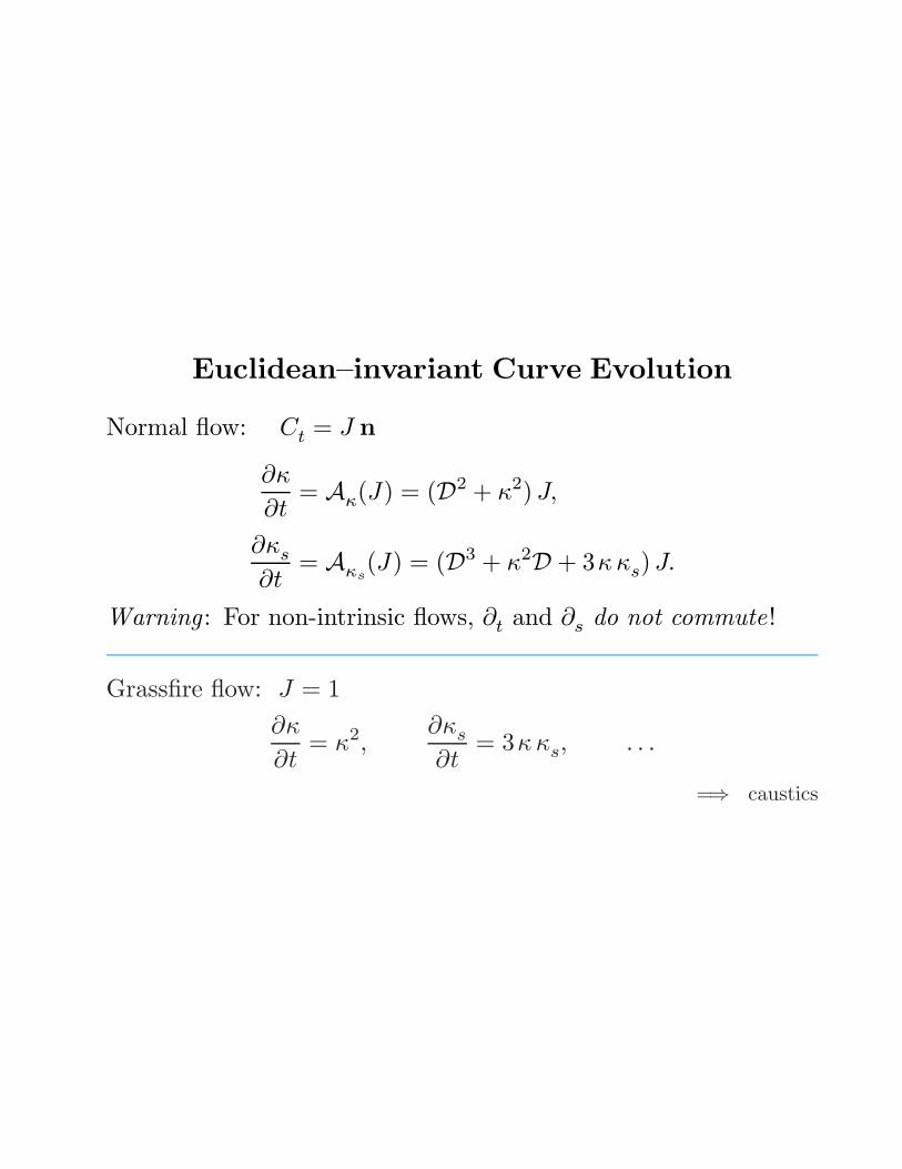
Euclidean–invariant Curve Evolution
Normal flow: Ct = J n
∂κ
∂t= Aκ(J) = (D2 + κ2) J,
∂κs
∂t= Aκs
(J) = (D3 + κ2D + 3κκs)J.
Warning : For non-intrinsic flows, ∂t and ∂s do not commute!
Grassfire flow: J = 1
∂κ
∂t= κ2,
∂κs
∂t= 3κκs, . . .
=⇒ caustics
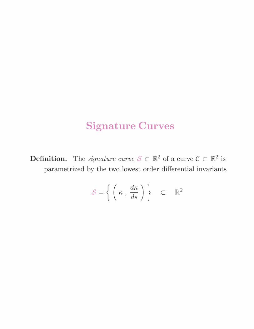
Signature Curves
Definition. The signature curve S ⊂ R2 of a curve C ⊂ R
2 is
parametrized by the two lowest order differential invariants
S =
(κ ,
dκ
ds
) ⊂ R
2
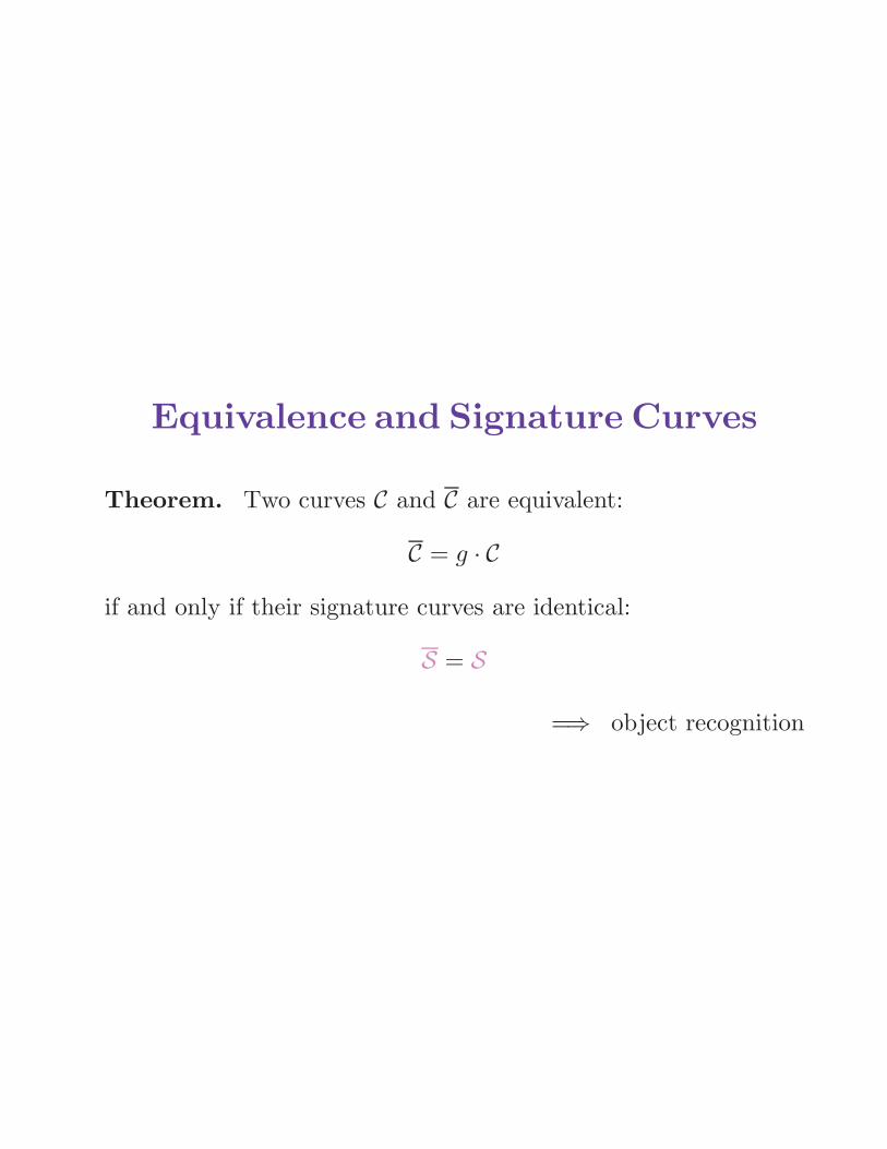
Equivalence and Signature Curves
Theorem. Two curves C and C are equivalent:
C = g · C
if and only if their signature curves are identical:
S = S
=⇒ object recognition
!"" #""
$#"
%""
%#"
&'()*
!"+"# " "+"# "+*!"+"*#
!"+"*
!"+""#
"
"+""#
"+"*
,-./0('12)3'142)&'()*
!"" #""
!#"
#""
##"
$""&'()5
!"+"# " "+"# "+*!"+"*#
!"+"*
!"+""#
"
"+""#
"+"*
,-./0('12)3'142)&'()5
!"+"# " "+"# "+*!"+"*#
!"+"*
!"+""#
"
"+""#
"+"*
36782/2889)"+*:%$%:
!""#""
$""
%""
&"""
'(()*&
!"+", " "+", "+&!"+"&,
!"+"&
!"+"",
"
"+"",
"+"&
-./012345*63475*'(()*&
8"" ,""
9,"
#""
#,"
:32*&
!"+", " "+", "+&!"+"&,
!"+"&
!"+"",
"
"+"",
"+"&
-./012345*63475*:32*&
!"+", " "+", "+&!"+"&,
!"+"&
!"+"",
"
"+"",
"+"&
6;(<505<<=*"+">&!&#
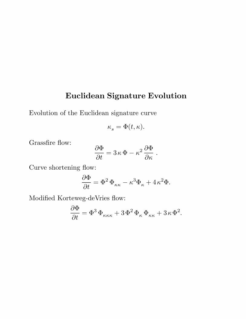
Euclidean Signature Evolution
Evolution of the Euclidean signature curve
κs = Φ(t, κ).
Grassfire flow:∂Φ
∂t= 3κΦ− κ2 ∂Φ
∂κ.
Curve shortening flow:
∂Φ
∂t= Φ2 Φκκ − κ3Φκ + 4κ2Φ.
Modified Korteweg-deVries flow:
∂Φ
∂t= Φ3 Φκκκ + 3Φ2 Φκ Φκκ + 3κΦ2.
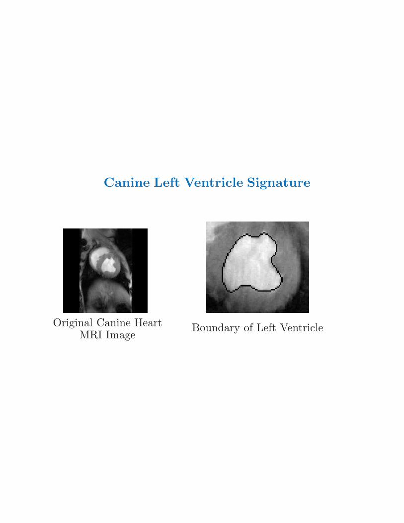
Canine Left Ventricle Signature
Original Canine HeartMRI Image
Boundary of Left Ventricle
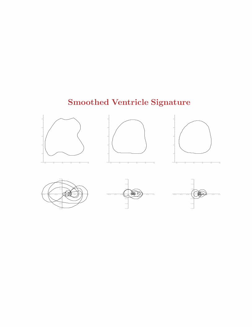
Smoothed Ventricle Signature
10 20 30 40 50 60
20
30
40
50
60
10 20 30 40 50 60
20
30
40
50
60
10 20 30 40 50 60
20
30
40
50
60
-0.15 -0.1 -0.05 0.05 0.1 0.15 0.2
-0.06
-0.04
-0.02
0.02
0.04
0.06
-0.15 -0.1 -0.05 0.05 0.1 0.15 0.2
-0.06
-0.04
-0.02
0.02
0.04
0.06
-0.15 -0.1 -0.05 0.05 0.1 0.15 0.2
-0.06
-0.04
-0.02
0.02
0.04
0.06
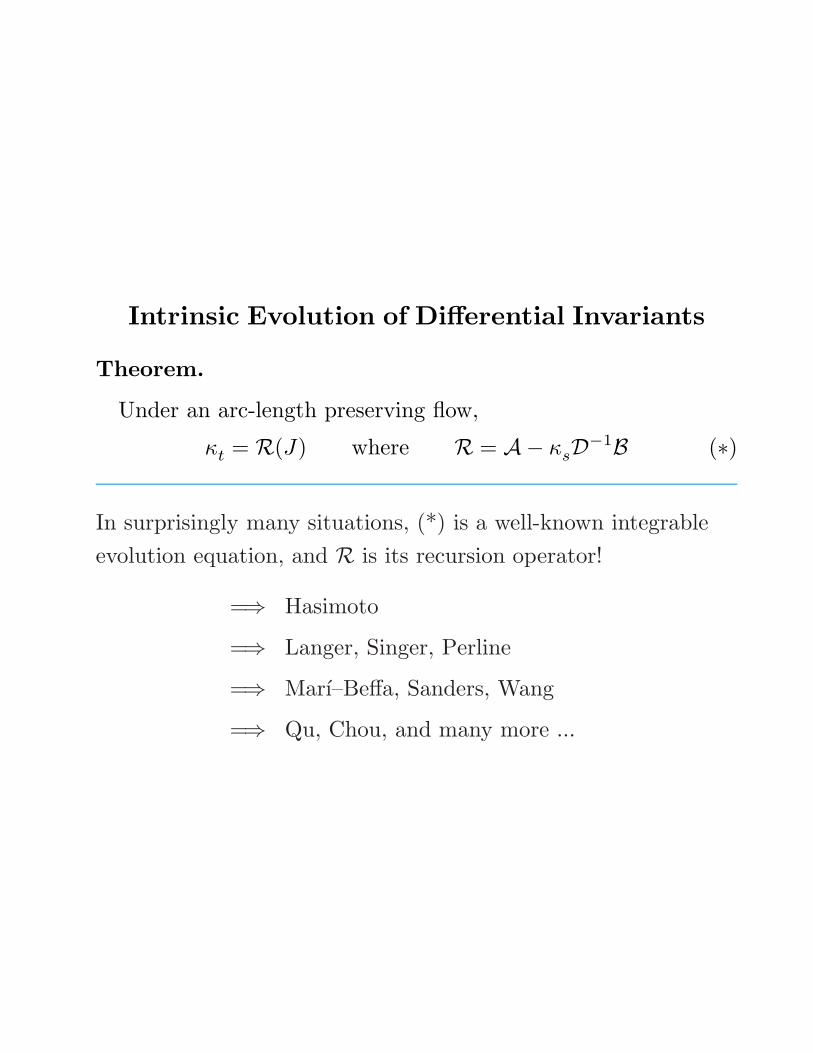
Intrinsic Evolution of Differential Invariants
Theorem.
Under an arc-length preserving flow,
κt = R(J) where R = A− κsD−1B (∗)
In surprisingly many situations, (*) is a well-known integrable
evolution equation, and R is its recursion operator!
=⇒ Hasimoto
=⇒ Langer, Singer, Perline
=⇒ Marı–Beffa, Sanders, Wang
=⇒ Qu, Chou, and many more ...
Euclidean plane curves
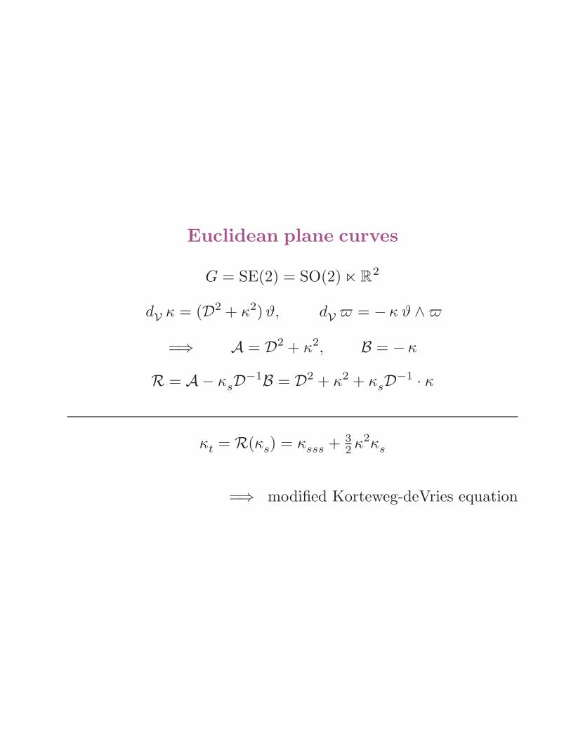
G = SE(2) = SO(2) ⋉ R2
dV
κ = (D2 + κ2) ϑ, dV
= −κ ϑ ∧
=⇒ A = D2 + κ2, B = −κ
R = A− κsD−1B = D2 + κ2 + κsD
−1 · κ
κt = R(κs) = κsss + 32 κ2κs
=⇒ modified Korteweg-deVries equation
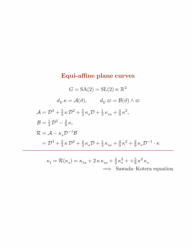
Equi-affine plane curves
G = SA(2) = SL(2) ⋉ R2
dV
κ = A(ϑ), dV
= B(ϑ) ∧
A = D4 + 53 κD2 + 5
3 κsD + 13 κss + 4
9 κ2,
B = 13 D
2 − 29 κ,
R = A− κsD−1B
= D4 + 53 κD2 + 4
3 κsD + 13 κss + 4
9 κ2 + 29 κsD
−1 · κ
κt = R(κs) = κ5s + 2κ κss + 43 κ2
s + +59 κ2 κs
=⇒ Sawada–Kotera equation
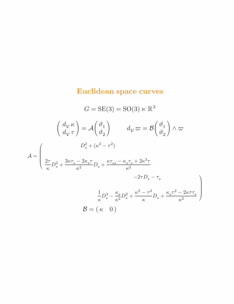
Euclidean space curves
G = SE(3) = SO(3) ⋉ R3
(dV
κdV
τ
)= A
(ϑ1
ϑ2
)dV
= B
(ϑ1
ϑ2
)∧
A =
D2s + (κ2 − τ2)
2τ
κD2
s +3κτs − 2κsτ
κ2Ds +
κτss − κsτs + 2κ3τ
κ2
−2τDs − τs
1
κD3
s −κs
κ2D2
s +κ2 − τ2
κDs +
κsτ2 − 2κττs
κ2
B = ( κ 0 )
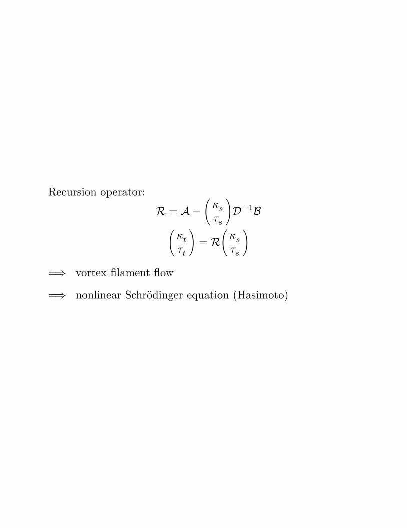
Recursion operator:
R = A−
(κs
τs
)D−1B
(κt
τt
)= R
(κs
τs
)
=⇒ vortex filament flow
=⇒ nonlinear Schrodinger equation (Hasimoto)


![Affine Geometry, Curve Flows, and Invariant Numerical ...Blaschke [6], who was inspired by Klein’s general Erlanger Programm, which provided the foundational link between groups](https://static.documents.pub/doc/80x56/6109f5ace6966a56a1660e43/affine-geometry-curve-flows-and-invariant-numerical-blaschke-6-who-was.jpg)