Submitted to Production and Operations Management manuscript POM-Jun-11-OA-0253 Inventory Rationing for Multiple Class Demand under Continuous Review Qing Ding School of Management, Huazhong University of Science and Technology [email protected]Panos Kouvelis Olin School of Business, Washington University in St. Louis, St. Louis, MO 63130 [email protected]Joseph Milner Rotman School of Management, University of Toronto, 105 St. George Street Toronto, ONT M5S 3E6 Canada [email protected]We consider how a firm should ration inventory to multiple classes in a stochastic demand environment with partial, class-dependent backlogging where the firm incurs a fixed setup cost when ordering from its supplier. We present an infinite-horizon, average cost criterion Markov decision process formulation for the case with zero lead times. We provide an algorithm that determines the optimal rationing policy, and show how to find the optimal base stock reorder policy. Numerical studies indicate that the optimal policy is similar to that given by the equivalent deterministic problem and relies on tracking both the current inventory and the rate that backorder costs are accumulating. Our study of the case of non-zero lead time shows that a heuristic combining the optimal, zero lead time policy with an allocation policy based on a single-period profit management problem is effective. 1. Introduction A common problem in distribution is the determination of which customers to serve when there is a limited supply of inventory. Often customers are characterized by the level of service they expect, either through explicit contracts or implicit in their business relationships. For example, by contract, suppliers may distinguish customers by the price they pay or the distribution channel they use. Alternatively, suppliers may characterize customers by the volume of business they engage in on an annual basis, preferring to provide higher levels of service to their best customers in expectation of furthering the relationship. A similar problem also occurs in production environments where the marginal value of a unit depends on its use. For example Dekker et al. (1998) discuss a case study on inventory control for spare parts in a large petrochemical plant, where parts are installed in equipment of different criticality. Other applications are given in the survey paper by Kleijn and Dekker (1999). The problem faced by the firm is to determine an inventory ordering policy from its supplier as well as a policy for allocating the capacity or inventory to different classes of customers. 1
Transcript
Submitted to Production and Operations Managementmanuscript POM-Jun-11-OA-0253
Inventory Rationing for Multiple Class Demandunder Continuous Review
Qing DingSchool of Management, Huazhong University of Science and Technology [email protected]
Panos KouvelisOlin School of Business, Washington University in St. Louis, St. Louis, MO 63130 [email protected]
Joseph MilnerRotman School of Management, University of Toronto, 105 St. George Street Toronto, ONT M5S 3E6 Canada
We consider how a firm should ration inventory to multiple classes in a stochastic demand environment with
partial, class-dependent backlogging where the firm incurs a fixed setup cost when ordering from its supplier.
We present an infinite-horizon, average cost criterion Markov decision process formulation for the case with
zero lead times. We provide an algorithm that determines the optimal rationing policy, and show how to
find the optimal base stock reorder policy. Numerical studies indicate that the optimal policy is similar to
that given by the equivalent deterministic problem and relies on tracking both the current inventory and
the rate that backorder costs are accumulating. Our study of the case of non-zero lead time shows that a
heuristic combining the optimal, zero lead time policy with an allocation policy based on a single-period
profit management problem is effective.
1. Introduction
A common problem in distribution is the determination of which customers to serve when there
is a limited supply of inventory. Often customers are characterized by the level of service they
expect, either through explicit contracts or implicit in their business relationships. For example, by
contract, suppliers may distinguish customers by the price they pay or the distribution channel they
use. Alternatively, suppliers may characterize customers by the volume of business they engage in on
an annual basis, preferring to provide higher levels of service to their best customers in expectation
of furthering the relationship. A similar problem also occurs in production environments where the
marginal value of a unit depends on its use. For example Dekker et al. (1998) discuss a case study
on inventory control for spare parts in a large petrochemical plant, where parts are installed in
equipment of different criticality. Other applications are given in the survey paper by Kleijn and
Dekker (1999). The problem faced by the firm is to determine an inventory ordering policy from its
supplier as well as a policy for allocating the capacity or inventory to different classes of customers.
1
Ding, Kouvelis, and Milner: Inventory Rationing for Multiple Class Demand2 Article submitted to Production and Operations Management; manuscript no. POM-Jun-11-OA-0253
In this paper we consider a single item, multiple class, continuous time inventory problem with
class-dependent partial backlogging and setup costs. A firm purchases inventory from a supplier,
incurring a fixed setup cost for each order it places. We consider Poisson unit demand (extending
to compound Poisson). For each arrival, the firm must determine whether to serve the demand
from stock, offer to backorder it and fill it from the next supply order, or place an order from
the supplier that, under a zero lead time assumption, will fill the demand. Each demand class
is characterized by a demand rate and a contribution margin per unit filled. Further, customer
classes are distinguished by the likelihood they will wait for demand fulfillment, if they are offered
to be backordered, and the cost per unit time of waiting for fulfillment. That is, there is partial,
class-dependent backordering where the backorder cost is proportional to the time until fulfillment.
We determine the optimal rationing and ordering policy to maximize the expected average profit
per unit time.
This paper contributes to the literature by providing an efficient algorithm to solve the
continuous-time inventory rationing model with setup costs. Previous work has considered (Q,R)
policies or single rationing thresholds based on inventory position and has only considered tracking
the total number of units backlogged. This makes sense in a single-class problem (or two-class
problem where only one class is backordered). However, in a multiple-class problem, the cost to a
firm of backlogging one customer versus another is likely to differ. For example, consider the cost
of backlogging an infrequent customer with low service expectations versus a high value customer
that a firm wishes to retain. Thus, we formulate the problem with the vector of backorders from
each class as a state variable. Further, our objective function generalizes the full backlogging case
to allow probabilistic customer acceptance of backlogging. However we show that we can collapse
the state space so that we only need to track the total backorder cost rate in order to determine the
optimal policy. We solve a dynamic program to maximize the single period profit when an auxiliary
operating cost per unit time is incurred and establish the structure of the optimal policy. We then
show that this solution, for an appropriately chosen operating cost, maximizes the average profit.
In particular we show that a (θi, I0) base-stock policy with class-dependent rationing is optimal
for the partial backlogging, infinite horizon case with an average profit criterion. That is, there
is a class-dependent threshold θi that determines the maximum backorder cost rate the firm will
incur prior to reordering and the firm orders to I0. As such it combines the previous work on
multiple-class rationing without setup costs with the approach to the price sensitive, continuous
time model of Feng and Chen (2003) and Chen and Simchi-Levi (2004a).
In addition, we show that the dynamic rationing policy provides insights into the problem. First,
classes are denied service in the order of the marginal benefit accrued if they wait for delayed
service, multiplied by the odds of their agreeing for such a delay. Thus inventory is protected
Ding, Kouvelis, and Milner: Inventory Rationing for Multiple Class DemandArticle submitted to Production and Operations Management; manuscript no. POM-Jun-11-OA-0253 3
for classes with a greater marginal benefit for immediate service. Further, we show that as the
inventory or total backorder cost rate increases, more classes are served from stock. Also, reorders
are not placed until inventory is depleted and then one must consider the class designation of
the arriving customer. A customer that is likely to wait for fulfillment and whose delay cost is
low, does not trigger a reorder. By delaying the reorder the firm can spread the fixed costs over a
greater number of customers, increasing the average profit. We show that the dynamic rationing
policy performs significantly better than a static policy when there are relatively few high valued
customers or when such customers are willing to wait for service.
In the next section we review the related literature. In Section 3 we present our model. We
then discuss its solution and provide proofs of the optimal policy in Section 4. In Section 5 we
compare the optimal policy to heuristics based on the deterministic policy to gain insight into
how the rationing policy performs. We discuss extensions to the model in Section 6. In particular,
throughout we assume that the firm incurs a class-dependent cost per unit time for all backordered
items. We note in our extensions that a class-dependent fixed cost per unit backordered can also
be accommodated by the model, with only minor changes to the results. We also discuss allowing
non-stationary probability of acceptance of the backorder and non-stationary backorder charges,
and compound Poisson demand. We address the assumption of a zero lead time for delivery from
the supplier in Section 7 by proposing a heuristic solution allowing a single outstanding order
with a positive lead time. The fundamental difficulty in including a positive lead time is that the
decisions on ordering and rationing take place on different time scales. Allowing for a positive
lead time would disrupt the renewal process we use to prove our results in that it would confound
the operational decisions of rationing with the periodic decision of reordering. This difficulty is
consistent with a similar one found in previous work in the (s,S, p) literature such as in Chen and
Simchi-Levi (2004a). We discuss our results in Section 8.
2. Literature Review
The paper links research on optimal rationing of inventory to multiple classes of customers with
work considering joint inventory and pricing policies. Both of these areas may be considered related
to the broader topic of revenue management (see Talluri and van Ryzin (2004) for a comprehensive
treatment of this literature). Topkis (1968) considers the rationing of inventory to multiple demand
classes in a periodic review model where a period is subdivided into several intervals. He shows
a class-dependent threshold, base-stock policy is optimal. Frank et al. (2003) extend the periodic
review problem to a multiple period problem with a deterministic priority class and a stochastic
secondary class. Ayvaz and Huh (2010) study an application of allocating hospital beds to two
classes of patients, one lost-sale and one backlogging. The capacity of each period is identical
Ding, Kouvelis, and Milner: Inventory Rationing for Multiple Class Demand4 Article submitted to Production and Operations Management; manuscript no. POM-Jun-11-OA-0253
on a finite horizon. Perhaps more relevant to the current work are several papers that consider
continuous time models. Nahmias and Demmy (1981) analyze a rationing policy with two-customer
classes and Poisson demand assuming a positive lead time and backorders. They study a (Q,R)
policy with rationing and a single outstanding order to evaluate fill rates for the classes. Moon
and Kang (1998) extend this model to a compound Poisson process demand. Melchiors et al.
(2000) consider a similar problem in a lost sales context. Deshpande et al. (2003) analyze a similar
problem to Nahmias and Demmy (1981) but allow for multiple outstanding orders. They consider
optimizing the (Q,R) inventory parameters and a backorder fulfillment policy to ration inventory.
Arslan et al. (2007) consider a model with multiple demand classes with service-level requirements.
The paper provides an efficient heuristic in a (Q,R) continuous review framework with rationing
to minimize the expected average on-hand inventory level on an infinite horizon.
Additional work has been conducted in production and inventory rationing contexts. Work such
as Ha (1997) considers inventory rationing to multiple classes for a make-to-stock production sys-
tem. Benjaafar and Elhafsi (2006) consider an assemble-to-order system with multiple customer
classes. Benjaafar et al. (2010) has recently studied a make-to-order system with partial backlog-
ging.
Other relevant research has considered the single-item price sensitive demand with setup costs.
Rather than rationing capacity to several classes, the demand rate is varied by changing the price.
Zheng (1991) provides an alternate proof of the optimality of a (s,S) policy as shown by Scarf
(1960), using the renewal reward argument we employ in this paper. Adopting this argument, Chen
and Simchi-Levi (2004c) show the optimality of a (s,S, p) policy where demand is controlled by
pricing in a periodic review model for a finite horizon with additive demand and backlogging. Chen
and Simchi-Levi (2004b) prove a similar result for the infinite-horizon case for both discounted-
profit and average profit. Feng and Chen (2003) and Chen and Simchi-Levi (2004a) show the
optimality of a (s,S, p) policy for the average profit case in a continuous review environment.
Recently, Huh and Janakiraman (2008) have developed an alternate approach for proving (s,S)
policies with demand control. This approach has been used in a context of multiplicative demand
and lost sales by Song et al. (2009).
The paper is also related to Ding et al. (2006) and Ding et al. (2007) which allow for discount-
based, partial backordering. Ding et al. (2006) consider a periodic review problem similar to the
problem studied by Topkis (1968). The authors assume the probability that a customer waits
for delayed demand fulfillment is based on a discount offered. As in Topkis (1968), the period
is divided into multiple stages, allowing updating of demand information and making allocation
decisions. They develop an algorithmic approach to determine the optimal allocation and discounts.
In comparison, Ding et al. (2007) consider a deterministic, multi-class inventory allocation model
Ding, Kouvelis, and Milner: Inventory Rationing for Multiple Class DemandArticle submitted to Production and Operations Management; manuscript no. POM-Jun-11-OA-0253 5
Table 1 Notation
λi Demand rate for class i, λ=∑λi
αi = λi/λri Class-i revenue per unitbi Class-i backorder cost per unit per unit timeγi Probability demand from class i accepts a backorderh Holding cost per unit per unit timeK Setup cost per orderφ Auxiliary cost per unit time incurredI Inventory~B Vector of number of backorders by classB Total backorder cost rate
ΠI, ~B Net profit for a single order starting in I, ~BT I,
~B Operating time for a single orderV I,Bi Profit-to-go in state (I,B) upon arrival of a class-i customer including φyI,Bi Variable indicating if class-i customers are served in state (I,B),
not served, or if an order is placed (1, 0, -1, respectively)
with partial backordering in an infinite horizon, EOQ-like setting. The paper provides closed-form
solutions to that case and insights into the drivers of firm policy. Among these it shows that both
high and low value customers can enjoy higher service rates and lower average delays through
the optimal policy compared with a first-come/first-served policy that offers discounts to retain
customers.
3. Model
We consider the problem faced by a firm that must determine when to purchase inventory from
a supplier and how to allocate the inventory to multiple customer classes in a continuous-review
environment. Customers are alternately served from stock or their demand is backlogged with same
probability. Each class is defined by its expected demand rate, contribution margin, likelihood to
accept a backlog, and backlogging cost.
Let N be the number of customer classes and let subscript i= 1, . . . ,N designate the class. We
assume customers from class-i arrive according to a Poisson process with rate λi and let λ=∑
i λi.
Let the probability an arrival is from class i be αi = λi/λ. Let ri be the revenue per unit, bi be the
backorder cost per unit per unit time, and γi be the probability a customer accepts a backlog. That
is, γibi expresses the expected cost per unit time of delaying a customer (the unit cost times the
probability a customer accepts a backlog), and γiri expresses the expected revenue from serving a
class-i customer from backlog. The constants γi and bi represent the outcome of a policy used to
encourage customers to accept delayed order fulfillment. We assume bi ∈N (the set of non-negative
integers).
Inventory held costs h per unit time. We assume that there is a fixed order setup cost for the firm,
K (typically relates to fixed costs of order generation and transportation), and that there is no lead
Ding, Kouvelis, and Milner: Inventory Rationing for Multiple Class Demand6 Article submitted to Production and Operations Management; manuscript no. POM-Jun-11-OA-0253
time for order fulfillment. The state of the system, s, is defined by the on-hand inventory, I, and the
vector of backlogged demands ~B = B1, . . . ,BN where Bi is the number of backlogged customers
from class i. That is, let s = I, ~B ∈ S =NN+1 be the state of the system. Let B =∑i∈N
biBi be
the total backorder cost rate in state s. Table 1 provides a summary of the notation; additional
notation will be defined as needed.
When a customer arrives, the firm must determine whether to serve the customer from stock,
deny the customer and perhaps serve the customer from backlog (delay the customer), or place an
order and serve the customer immediately from the order (reorder). At an arrival epoch of a class-i
customer at time t, let ai(s) = yi(s), zi(s) be the action in state s= I, ~B where
yi(s) =
1 if a class-i customer is served in state s0 if a class-i customer is delayed in state s−1 if a reorder is placed upon the arrival of a class-i customer in state s
(1)
and zi(s) is the on-hand inventory after a purchase is made in state s. That is, if yi(s) =−1, the
resulting state is s′ = I ′, ~B′ where I ′ = zi(s) and 0 ≤ B′j ≤ Bj for all j ∈ N . (We show below
B′j = 0 for all j (all backorders are filled), and so for simplicity of notation write the action as
ai(s) = yi(s), zi(s) as opposed to clarifying the decision on how to treat the backorders.)
The expected revenue received in state s for decision yi(s) is
r(s, ai(s)) =
ri yi(s) = 1γiri yi(s) = 0ri yi(s) =−1
(2)
and the expected cost rate incurred by the firm from the arrival to state S under decision ai(s) is
Let π be some policy yπ(s), zπ(s). Let Xit>0 be the Poisson arrival process for class-i and
let Xt>0 be the vector of arrival processes for all classes. Let x be realization of Xt>0. Let
σ = I0,B0 be the state of the system at time t = 0. Let Σn(x) be the time of the nth arrival
from all classes and let νt(x) be the number of arrivals from all classes by time t. Define ν0 = 0
(we assume no arrivals at time t= 0). Let sπ,σn (x) be the state of the system at the time of the nth
arrival, given policy π, initial state σ and arrival process realization x∈X.
Then suppressing the dependence of sπ,σn on x, we can define the expected revenue received from
the nth arrival as
rπ,σn (x) = r(sπ,σn , a(sπ,σn ))
and the inventory and backorder cost incurred for t, Σn(x)≤ t <Σn+1(x) as
cπ,σt (x) = c(sπ,σνt , a(sπ,σνt ))
Ding, Kouvelis, and Milner: Inventory Rationing for Multiple Class DemandArticle submitted to Production and Operations Management; manuscript no. POM-Jun-11-OA-0253 7
(note cπ,σt (x) = hI +B for σ= I, ~B,0≤ t <Σn+1(x)).
We define a cycle as the time between placing orders, that is, if for some arrival time Σn,
y(sπ,σn ) =−1, and for some integer m>n,y(sπ,σm ) =−1, and y(sπ,σk ) 6=−1 for all k, n< k <m, then a
cycle starts at Σn and finishes at Σm. We define the first cycle to start at t= 0. Let T π,σM (x)≡Σn(x)
be the time to complete M cycles, where the nth arrival completes the M th cycle.
Let uπ,σM (x) = νTπ,σM
be the number of arrivals at the completion of the M th cycle. Note that
T π,σM (x) is a stopping time so that we can take expectations over all X until time T π,σM (x) and
similarly until the uπ,σM (x)th arrival. Then the expected profit received under policy π over M cycles
with initial state σ is defined as
vπ,σM ≡EX
uπ,σM (x)∑n=1
rπ,σn (x)−∫ T
π,σM
(x)
0
cπ,σt (x)dt−MK
. (4)
The profit expresses the total revenue received over M cycles less the inventory and backorder
costs incurred less the total setup costs over the M cycles. The average reward for policy π given
initial state σ is defined as
hπ,σ ≡ limM→∞
vπ,σME [T π,σM (x)]
(5)
We solve for the policy π∗ that maximizes hπ,σ.
3.1. Discussion of Assumptions
In the formulation we have made the implicit assumption that reorders do not take place between
arrivals. This is without loss of generality. First, because of the Poisson assumption, reorders would
only take place either when a customer arrives, or immediately after that customer is served or
delayed. Observe that if a customer is served, the firm could instead have placed an order and
served the customer from the reorder. Thus serving a customer from stock and then reordering
immediately is equivalent to just reordering. On the other hand, if a customer is delayed, the
firm receives expected revenue γiri which is less than ri, the revenue received from reordering. So
delaying the customer, and then reordering immediately if they choose to stay, has lower expected
value than just reordering.
Similar to other backlogging models, we assume that backlogged customers orders are filled
through a reorder and not from inventory. While there may be instances where a firm would prefer
to fill a backlogged customer earlier than from the next reorder, the benefit in doing so is to lower
the backlog cost, and not increase revenue as the revenue of a backlogged customer has already
been recognized. Thus, a firm would do so only if the backlogging cost, bi, was high. Observe, if bi
were high, the firm would backlog the customer only if there were a small chance of acceptance, γi.
Ding, Kouvelis, and Milner: Inventory Rationing for Multiple Class Demand8 Article submitted to Production and Operations Management; manuscript no. POM-Jun-11-OA-0253
Further, high bi would tend to be associated with high revenue customers, ri, further supporting
the assumption. We note that in the case of high ri, it is unlikely that a customer would have been
backlogged at all. To summarize, it is possible for a firm to prefer to fill a backlog from inventory,
but it would seem unlikely to find itself in such a situation.
It is also possible that the firm may offer a backorder to a customer, hoping that they reject
it. A consequence of the preceding assumption is that if the customer chooses to be backordered,
then it might be beneficial for the firm to subsequently place a new order to fill the backordered
customers, even while holding inventory. To prove the optimality of our policy, and in particular
the non-optimality of ordering while holding inventory, we assume bi < λE[(1− γj)rj] + h for all
customer classes i. That is, the backlogging cost rate for all customers is less than the expected
lost sales cost rate of future demand plus the holding cost. Similar to the preceding argument, the
firm is unlikely to backorder customers if this inequality does not hold, i.e., if bi is high, γi is close
to 1, and ri is high. Thus the assumption is not overly restrictive. However, if it does not hold, the
policy given below would be approximately correct, filling orders from stock instead of by reorder,
ensuring the backorder cost did not increase.
As noted we address several extensions allowing various additional costs, state-dependent param-
eters, and compound Poisson demand in Section 6. We address the assumption of zero lead time
in Section 7.
4. Solution Approach
We approach the problem by first considering a single period version of the problem of maximizing
the expected profit where an additional exogenous operating cost, φ, is charged per unit time.
Assuming an initial inventory we find the optimal allocation policy and initial backorder values
for the single period problem by first considering the problem on a reduced state space tracking
only the total backorder cost rate. We then show the resulting policy also solves the single period
problem on the full state space. Next we find the optimal initial inventory level for the single period
problem. We then show that any optimal policy for the infinite period, average profit maximizing
problem, defines a renewal process. Finally we establish that the policy that maximizes (5) is given
by a policy that maximizes the optimal single period profit for an appropriately chosen value of φ.
4.1. Single Period Problem
Consider the following single period problem. As above, customers arrive from N classes according
to independent Poisson processes with associated parameters λi, ri, bi and γi. Similar to above, for
each arrival the firm must choose whether to serve, delay, or, in this case of a single period, close
the firm. As above let the state s= I, ~B and let yi(s) be the action taken in state s as defined
in (1) though now we redefine yi(s) =−1 to indicate the firm is closed in state s upon the arrival
Ding, Kouvelis, and Milner: Inventory Rationing for Multiple Class DemandArticle submitted to Production and Operations Management; manuscript no. POM-Jun-11-OA-0253 9
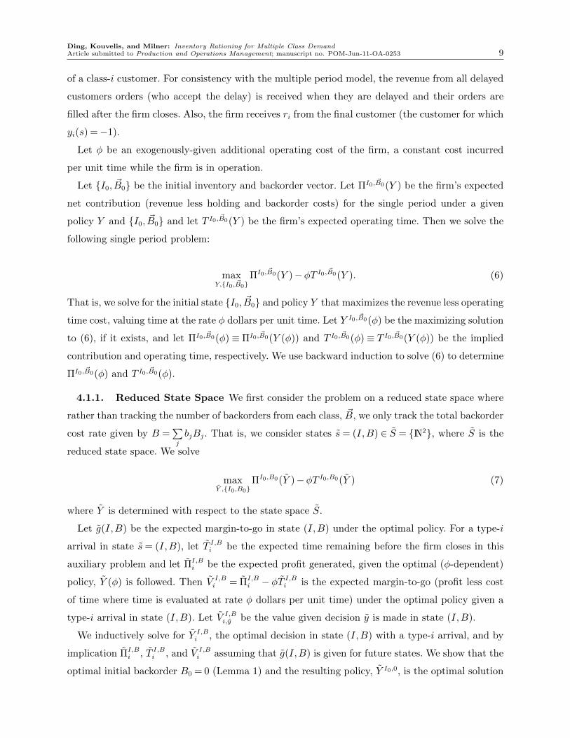
of a class-i customer. For consistency with the multiple period model, the revenue from all delayed
customers orders (who accept the delay) is received when they are delayed and their orders are
filled after the firm closes. Also, the firm receives ri from the final customer (the customer for which
yi(s) =−1).
Let φ be an exogenously-given additional operating cost of the firm, a constant cost incurred
per unit time while the firm is in operation.
Let I0, ~B0 be the initial inventory and backorder vector. Let ΠI0, ~B0(Y ) be the firm’s expected
net contribution (revenue less holding and backorder costs) for the single period under a given
policy Y and I0, ~B0 and let T I0,~B0(Y ) be the firm’s expected operating time. Then we solve the
following single period problem:
maxY,I0, ~B0
ΠI0, ~B0(Y )−φT I0, ~B0(Y ). (6)
That is, we solve for the initial state I0, ~B0 and policy Y that maximizes the revenue less operating
time cost, valuing time at the rate φ dollars per unit time. Let Y I0, ~B0(φ) be the maximizing solution
to (6), if it exists, and let ΠI0, ~B0(φ)≡ ΠI0, ~B0(Y (φ)) and T I0,~B0(φ)≡ T I0, ~B0(Y (φ)) be the implied
contribution and operating time, respectively. We use backward induction to solve (6) to determine
ΠI0, ~B0(φ) and T I0,~B0(φ).
4.1.1. Reduced State Space We first consider the problem on a reduced state space where
rather than tracking the number of backorders from each class, ~B, we only track the total backorder
cost rate given by B =∑j
bjBj. That is, we consider states s= (I,B) ∈ S = N2, where S is the
reduced state space. We solve
maxY ,I0,B0
ΠI0,B0(Y )−φT I0,B0(Y ) (7)
where Y is determined with respect to the state space S.
Let g(I,B) be the expected margin-to-go in state (I,B) under the optimal policy. For a type-i
arrival in state s= (I,B), let T I,Bi be the expected time remaining before the firm closes in this
auxiliary problem and let ΠI,Bi be the expected profit generated, given the optimal (φ-dependent)
policy, Y (φ) is followed. Then V I,Bi = ΠI,B
i − φT I,Bi is the expected margin-to-go (profit less cost
of time where time is evaluated at rate φ dollars per unit time) under the optimal policy given a
type-i arrival in state (I,B). Let V I,Bi,y be the value given decision y is made in state (I,B).
We inductively solve for Y I,Bi , the optimal decision in state (I,B) with a type-i arrival, and by
implication ΠI,Bi , T I,Bi , and V I,B
i assuming that g(I,B) is given for future states. We show that the
optimal initial backorder B0 = 0 (Lemma 1) and the resulting policy, Y I0,0, is the optimal solution
Ding, Kouvelis, and Milner: Inventory Rationing for Multiple Class Demand10 Article submitted to Production and Operations Management; manuscript no. POM-Jun-11-OA-0253
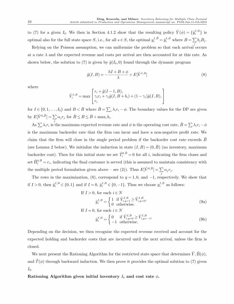
to (7) for a given I0. We then in Section 4.1.2 show that the resulting policy Y (φ) = yI,Bi is
optimal also for the full state space S, i.e., for all s∈ S, the optimal yI,~B
i = yI,Bi where B =∑j
bjBj.
Relying on the Poisson assumption, we can uniformize the problem so that each arrival occurs
at a rate λ and the expected revenue and costs per arrival are then accounted for at this rate. As
shown below, the solution to (7) is given by g(I0,0) found through the dynamic program
∑i λiri−φ. The boundary values for the DP are given
by E[V 0,B] =∑j
αjrj for B ≤B ≤ B+ maxi bi.
As∑λiri is the maximum expected revenue rate and φ is the operating cost rate, B =
∑λiri−φ
is the maximum backorder rate that the firm can incur and have a non-negative profit rate. We
claim that the firm will close in the single period problem if the backorder cost rate exceeds B
(see Lemma 2 below). We initialize the induction in state (I,B) = (0, B) (no inventory, maximum
backorder cost). Then for this initial state we set T 0,Bi = 0 for all i, indicating the firm closes and
set Π0,Bi = ri, indicating the final customer is served (this is assumed to maintain consistency with
the multiple period formulation given above – see (2)). Thus E[V 0,B] =∑j
αjrj.
The rows in the maximization, (8), correspond to y = 1,0, and −1, respectively. We show that
if I > 0, then yI,Bi ∈ 0,1 and if I = 0, yI,Bi ∈ 0,−1. Thus we choose yI,Bi as follows:
If I > 0, for each i∈N
yI,Bi =
1 if V I,B
i,y=1 ≥ VI,Bi,y=0,
0 otherwise.(9a)
If I = 0, for each i∈N
yI,Bi =
0 if V I,B
i,y=0 ≥ VI,Bi,y=−1,
−1 otherwise.(9b)
Depending on the decision, we then recognize the expected revenue received and account for the
expected holding and backorder costs that are incurred until the next arrival, unless the firm is
closed.
We next present the Rationing Algorithm for the restricted state space that determines Y , Π(φ),
and T (φ) through backward induction. We then prove it provides the optimal solution to (7) given
I0.
Rationing Algorithm given initial inventory I0 and cost rate φ.
Ding, Kouvelis, and Milner: Inventory Rationing for Multiple Class DemandArticle submitted to Production and Operations Management; manuscript no. POM-Jun-11-OA-0253 11
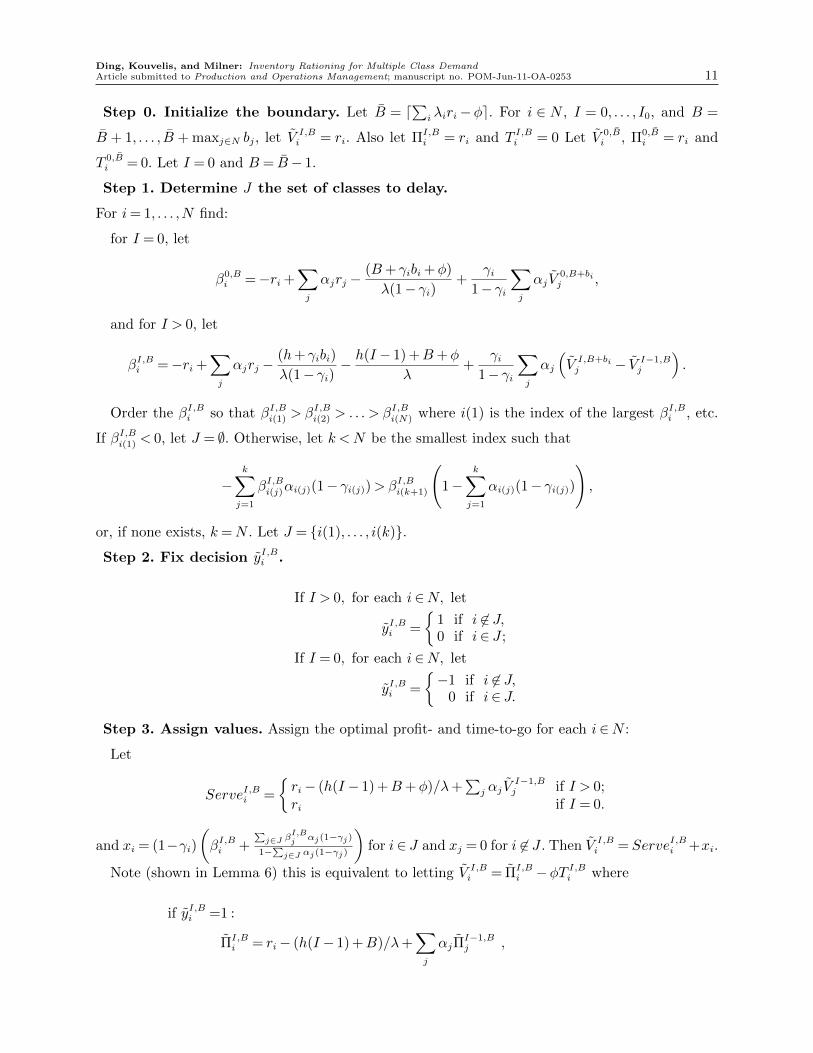
Step 0. Initialize the boundary. Let B = d∑
i λiri−φe. For i ∈ N , I = 0, . . . , I0, and B =
B + 1, . . . , B + maxj∈N bj, let V I,Bi = ri. Also let ΠI,B
i = ri and T I,Bi = 0 Let V 0,Bi , Π0,B
i = ri and
T 0,Bi = 0. Let I = 0 and B = B− 1.
Step 1. Determine J the set of classes to delay.
For i= 1, . . . ,N find:
for I = 0, let
β0,Bi =−ri +
∑j
αjrj −(B+ γibi +φ)
λ(1− γi)+
γi1− γi
∑j
αjV0,B+bij ,
and for I > 0, let
βI,Bi =−ri +∑j
αjrj −(h+ γibi)
λ(1− γi)− h(I − 1) +B+φ
λ+
γi1− γi
∑j
αj
(V I,B+bij − V I−1,B
j
).
Order the βI,Bi so that βI,Bi(1) > βI,Bi(2) > . . . > βI,Bi(N) where i(1) is the index of the largest βI,Bi , etc.
If βI,Bi(1) < 0, let J = ∅. Otherwise, let k <N be the smallest index such that
−k∑j=1
βI,Bi(j)αi(j)(1− γi(j))>βI,Bi(k+1)
(1−
k∑j=1
αi(j)(1− γi(j))
),
or, if none exists, k=N . Let J = i(1), . . . , i(k).
Step 2. Fix decision yI,Bi .
If I > 0, for each i∈N, let
yI,Bi =
1 if i 6∈ J,0 if i∈ J ;
If I = 0, for each i∈N, let
yI,Bi =
−1 if i 6∈ J,
0 if i∈ J.
Step 3. Assign values. Assign the optimal profit- and time-to-go for each i∈N :
Let
ServeI,Bi =
ri− (h(I − 1) +B+φ)/λ+
∑j αjV
I−1,Bj if I > 0;
ri if I = 0.
and xi = (1−γi)(βI,Bi +
∑j∈J β
I,Bj αj(1−γj)
1−∑j∈J αj(1−γj)
)for i∈ J and xj = 0 for i 6∈ J . Then V I,B
i = ServeI,Bi +xi.
Note (shown in Lemma 6) this is equivalent to letting V I,Bi = ΠI,B
i −φT I,Bi where
if yI,Bi =1 :
ΠI,Bi = ri− (h(I − 1) +B)/λ+
∑j
αjΠI−1,Bj ,
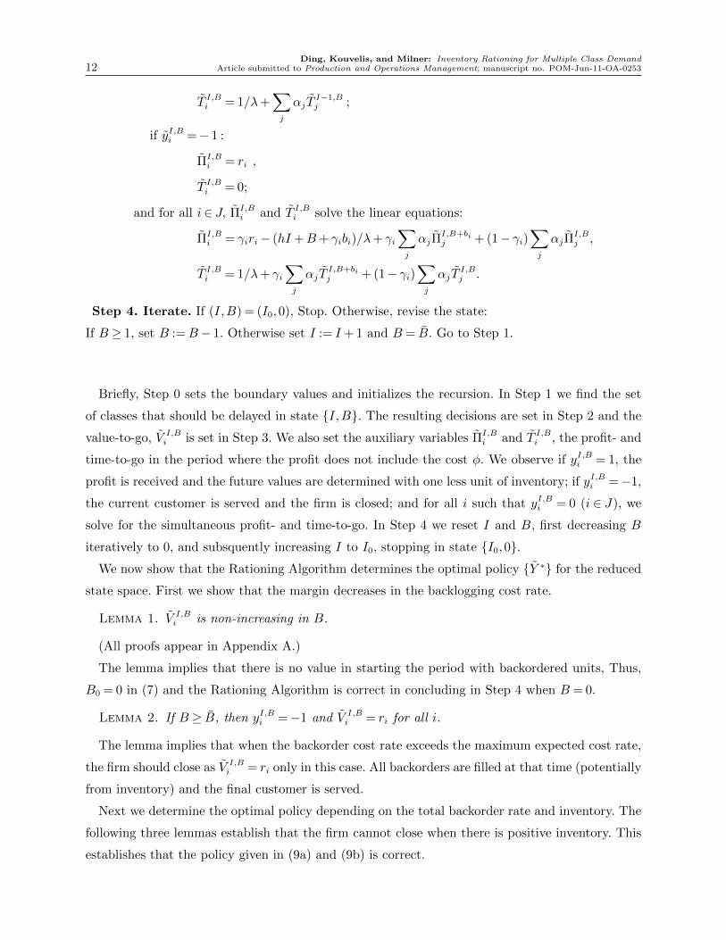
Ding, Kouvelis, and Milner: Inventory Rationing for Multiple Class Demand12 Article submitted to Production and Operations Management; manuscript no. POM-Jun-11-OA-0253
T I,Bi = 1/λ+∑j
αjTI−1,Bj ;
if yI,Bi =− 1 :
ΠI,Bi = ri ,
T I,Bi = 0;
and for all i∈ J, ΠI,Bi and T I,Bi solve the linear equations:
ΠI,Bi = γiri− (hI +B+ γibi)/λ+ γi
∑j
αjΠI,B+bij + (1− γi)
∑j
αjΠI,Bj ,
T I,Bi = 1/λ+ γi∑j
αjTI,B+bij + (1− γi)
∑j
αjTI,Bj .
Step 4. Iterate. If (I,B) = (I0,0), Stop. Otherwise, revise the state:
If B ≥ 1, set B :=B− 1. Otherwise set I := I + 1 and B = B. Go to Step 1.
Briefly, Step 0 sets the boundary values and initializes the recursion. In Step 1 we find the set
of classes that should be delayed in state I,B. The resulting decisions are set in Step 2 and the
value-to-go, V I,Bi is set in Step 3. We also set the auxiliary variables ΠI,B
i and T I,Bi , the profit- and
time-to-go in the period where the profit does not include the cost φ. We observe if yI,Bi = 1, the
profit is received and the future values are determined with one less unit of inventory; if yI,Bi =−1,
the current customer is served and the firm is closed; and for all i such that yI,Bi = 0 (i ∈ J), we
solve for the simultaneous profit- and time-to-go. In Step 4 we reset I and B, first decreasing B
iteratively to 0, and subsquently increasing I to I0, stopping in state I0,0.We now show that the Rationing Algorithm determines the optimal policy Y ∗ for the reduced
state space. First we show that the margin decreases in the backlogging cost rate.
Lemma 1. V I,Bi is non-increasing in B.
(All proofs appear in Appendix A.)
The lemma implies that there is no value in starting the period with backordered units, Thus,
B0 = 0 in (7) and the Rationing Algorithm is correct in concluding in Step 4 when B = 0.
Lemma 2. If B ≥ B, then yI,Bi =−1 and V I,Bi = ri for all i.
The lemma implies that when the backorder cost rate exceeds the maximum expected cost rate,
the firm should close as V I,Bi = ri only in this case. All backorders are filled at that time (potentially
from inventory) and the final customer is served.
Next we determine the optimal policy depending on the total backorder rate and inventory. The
following three lemmas establish that the firm cannot close when there is positive inventory. This
establishes that the policy given in (9a) and (9b) is correct.
Ding, Kouvelis, and Milner: Inventory Rationing for Multiple Class DemandArticle submitted to Production and Operations Management; manuscript no. POM-Jun-11-OA-0253 13
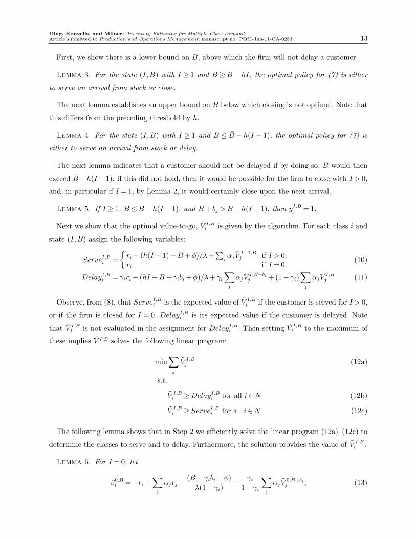
First, we show there is a lower bound on B, above which the firm will not delay a customer.
Lemma 3. For the state (I,B) with I ≥ 1 and B ≥ B − hI, the optimal policy for (7) is either
to serve an arrival from stock or close.
The next lemma establishes an upper bound on B below which closing is not optimal. Note that
this differs from the preceding threshold by h.
Lemma 4. For the state (I,B) with I ≥ 1 and B ≤ B − h(I − 1), the optimal policy for (7) is
either to serve an arrival from stock or delay.
The next lemma indicates that a customer should not be delayed if by doing so, B would then
exceed B−h(I−1). If this did not hold, then it would be possible for the firm to close with I > 0,
and, in particular if I = 1, by Lemma 2, it would certainly close upon the next arrival.
Lemma 5. If I ≥ 1, B ≤ B−h(I − 1), and B+ bj > B−h(I − 1), then yI,Bj = 1.
Next we show that the optimal value-to-go, V I,Bi is given by the algorithm. For each class i and
state (I,B) assign the following variables:
ServeI,Bi =
ri− (h(I − 1) +B+φ)/λ+
∑j αjV
I−1,Bj if I > 0;
ri if I = 0.(10)
DelayI,Bi = γiri− (hI +B+ γibi +φ)/λ+ γi∑j
αjVI,B+bij + (1− γi)
∑j
αjVI,Bj (11)
Observe, from (8), that ServeI,Bi is the expected value of V I,Bi if the customer is served for I > 0,
or if the firm is closed for I = 0. DelayI,Bi is its expected value if the customer is delayed. Note
that V I,Bj is not evaluated in the assignment for DelayI,Bi . Then setting V I,B
i to the maximum of
these implies V I,B solves the following linear program:
min∑j
V I,Bj (12a)
s.t.
V I,Bi ≥DelayI,Bi for all i∈N (12b)
V I,Bi ≥ ServeI,Bi for all i∈N (12c)
The following lemma shows that in Step 2 we efficiently solve the linear program (12a)–(12c) to
determine the classes to serve and to delay. Furthermore, the solution provides the value of V I,Bi .
Lemma 6. For I = 0, let
β0,Bi =−ri +
∑j
αjrj −(B+ γibi +φ)
λ(1− γi)+
γi1− γi
∑j
αjV0,B+bij , (13)
Ding, Kouvelis, and Milner: Inventory Rationing for Multiple Class Demand14 Article submitted to Production and Operations Management; manuscript no. POM-Jun-11-OA-0253
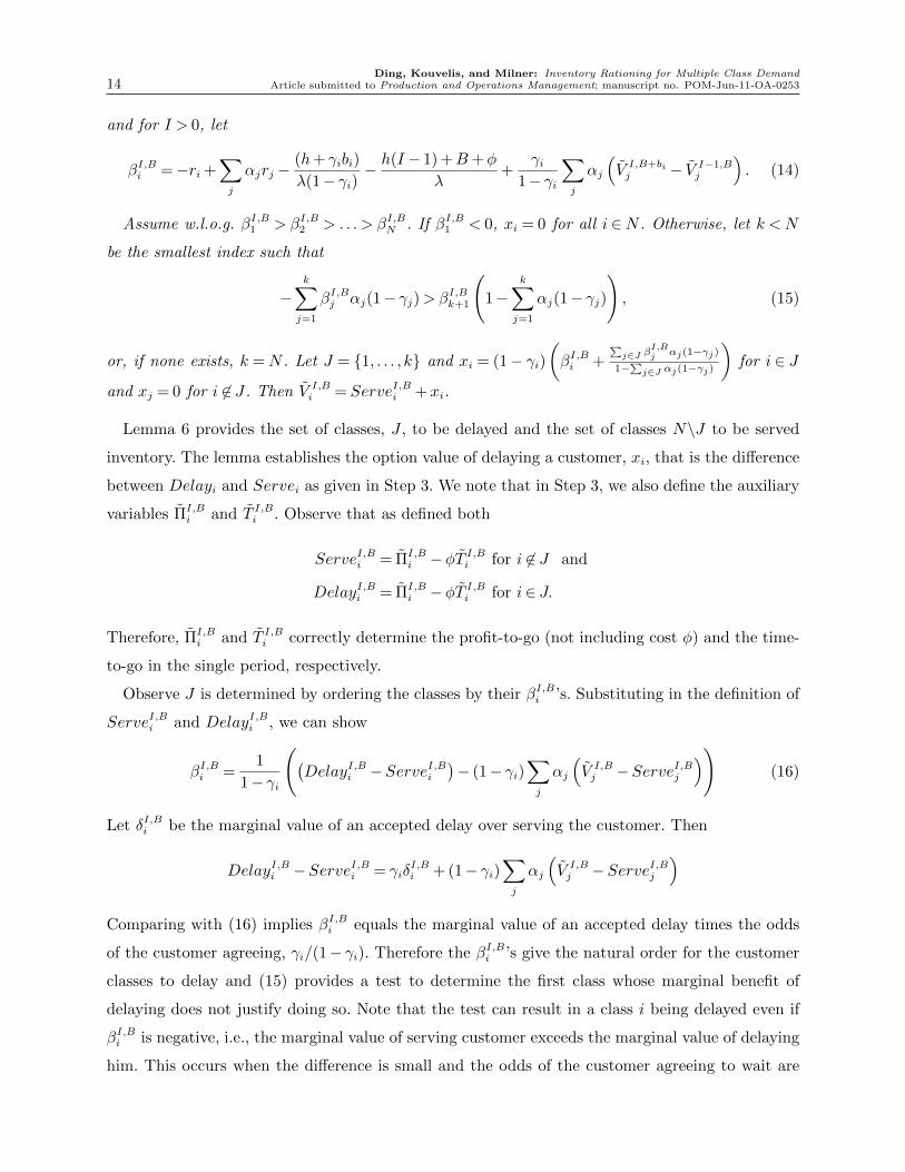
and for I > 0, let
βI,Bi =−ri +∑j
αjrj −(h+ γibi)
λ(1− γi)− h(I − 1) +B+φ
λ+
γi1− γi
∑j
αj
(V I,B+bij − V I−1,B
j
). (14)
Assume w.l.o.g. βI,B1 > βI,B2 > . . . > βI,BN . If βI,B1 < 0, xi = 0 for all i ∈N . Otherwise, let k <N
be the smallest index such that
−k∑j=1
βI,Bj αj(1− γj)>βI,Bk+1
(1−
k∑j=1
αj(1− γj)
), (15)
or, if none exists, k =N . Let J = 1, . . . , k and xi = (1− γi)(βI,Bi +
∑j∈J β
I,Bj αj(1−γj)
1−∑j∈J αj(1−γj)
)for i ∈ J
and xj = 0 for i 6∈ J . Then V I,Bi = ServeI,Bi +xi.
Lemma 6 provides the set of classes, J , to be delayed and the set of classes N\J to be served
inventory. The lemma establishes the option value of delaying a customer, xi, that is the difference
between Delayi and Servei as given in Step 3. We note that in Step 3, we also define the auxiliary
variables ΠI,Bi and T I,Bi . Observe that as defined both
ServeI,Bi = ΠI,Bi −φT I,Bi for i 6∈ J and
DelayI,Bi = ΠI,Bi −φT I,Bi for i∈ J.
Therefore, ΠI,Bi and T I,Bi correctly determine the profit-to-go (not including cost φ) and the time-
to-go in the single period, respectively.
Observe J is determined by ordering the classes by their βI,Bi ’s. Substituting in the definition of
ServeI,Bi and DelayI,Bi , we can show
βI,Bi =1
1− γi
((DelayI,Bi −ServeI,Bi
)− (1− γi)
∑j
αj
(V I,Bj −ServeI,Bj
))(16)
Let δI,Bi be the marginal value of an accepted delay over serving the customer. Then
DelayI,Bi −ServeI,Bi = γiδI,Bi + (1− γi)
∑j
αj
(V I,Bj −ServeI,Bj
)Comparing with (16) implies βI,Bi equals the marginal value of an accepted delay times the odds
of the customer agreeing, γi/(1− γi). Therefore the βI,Bi ’s give the natural order for the customer
classes to delay and (15) provides a test to determine the first class whose marginal benefit of
delaying does not justify doing so. Note that the test can result in a class i being delayed even if
βI,Bi is negative, i.e., the marginal value of serving customer exceeds the marginal value of delaying
him. This occurs when the difference is small and the odds of the customer agreeing to wait are
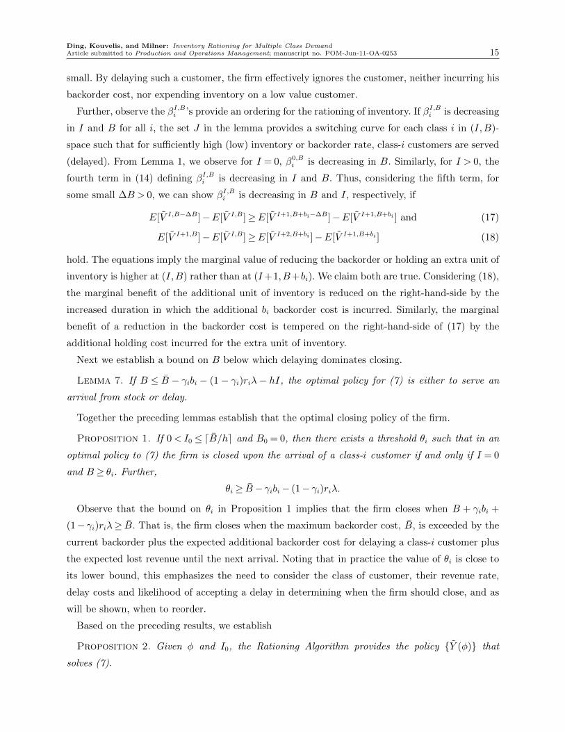
Ding, Kouvelis, and Milner: Inventory Rationing for Multiple Class DemandArticle submitted to Production and Operations Management; manuscript no. POM-Jun-11-OA-0253 15
small. By delaying such a customer, the firm effectively ignores the customer, neither incurring his
backorder cost, nor expending inventory on a low value customer.
Further, observe the βI,Bi ’s provide an ordering for the rationing of inventory. If βI,Bi is decreasing
in I and B for all i, the set J in the lemma provides a switching curve for each class i in (I,B)-
space such that for sufficiently high (low) inventory or backorder rate, class-i customers are served
(delayed). From Lemma 1, we observe for I = 0, β0,Bi is decreasing in B. Similarly, for I > 0, the
fourth term in (14) defining βI,Bi is decreasing in I and B. Thus, considering the fifth term, for
some small ∆B > 0, we can show βI,Bi is decreasing in B and I, respectively, if
E[V I,B−∆B]−E[V I,B]≥E[V I+1,B+bi−∆B]−E[V I+1,B+bi ] and (17)
hold. The equations imply the marginal value of reducing the backorder or holding an extra unit of
inventory is higher at (I,B) rather than at (I+1,B+bi). We claim both are true. Considering (18),
the marginal benefit of the additional unit of inventory is reduced on the right-hand-side by the
increased duration in which the additional bi backorder cost is incurred. Similarly, the marginal
benefit of a reduction in the backorder cost is tempered on the right-hand-side of (17) by the
additional holding cost incurred for the extra unit of inventory.
Next we establish a bound on B below which delaying dominates closing.
Lemma 7. If B ≤ B − γibi − (1− γi)riλ− hI, the optimal policy for (7) is either to serve an
arrival from stock or delay.
Together the preceding lemmas establish that the optimal closing policy of the firm.
Proposition 1. If 0< I0 ≤ dB/he and B0 = 0, then there exists a threshold θi such that in an
optimal policy to (7) the firm is closed upon the arrival of a class-i customer if and only if I = 0
and B ≥ θi. Further,
θi ≥ B− γibi− (1− γi)riλ.
Observe that the bound on θi in Proposition 1 implies that the firm closes when B + γibi +
(1− γi)riλ≥ B. That is, the firm closes when the maximum backorder cost, B, is exceeded by the
current backorder plus the expected additional backorder cost for delaying a class-i customer plus
the expected lost revenue until the next arrival. Noting that in practice the value of θi is close to
its lower bound, this emphasizes the need to consider the class of customer, their revenue rate,
delay costs and likelihood of accepting a delay in determining when the firm should close, and as
will be shown, when to reorder.
Based on the preceding results, we establish
Proposition 2. Given φ and I0, the Rationing Algorithm provides the policy Y (φ) that
solves (7).
Ding, Kouvelis, and Milner: Inventory Rationing for Multiple Class Demand16 Article submitted to Production and Operations Management; manuscript no. POM-Jun-11-OA-0253
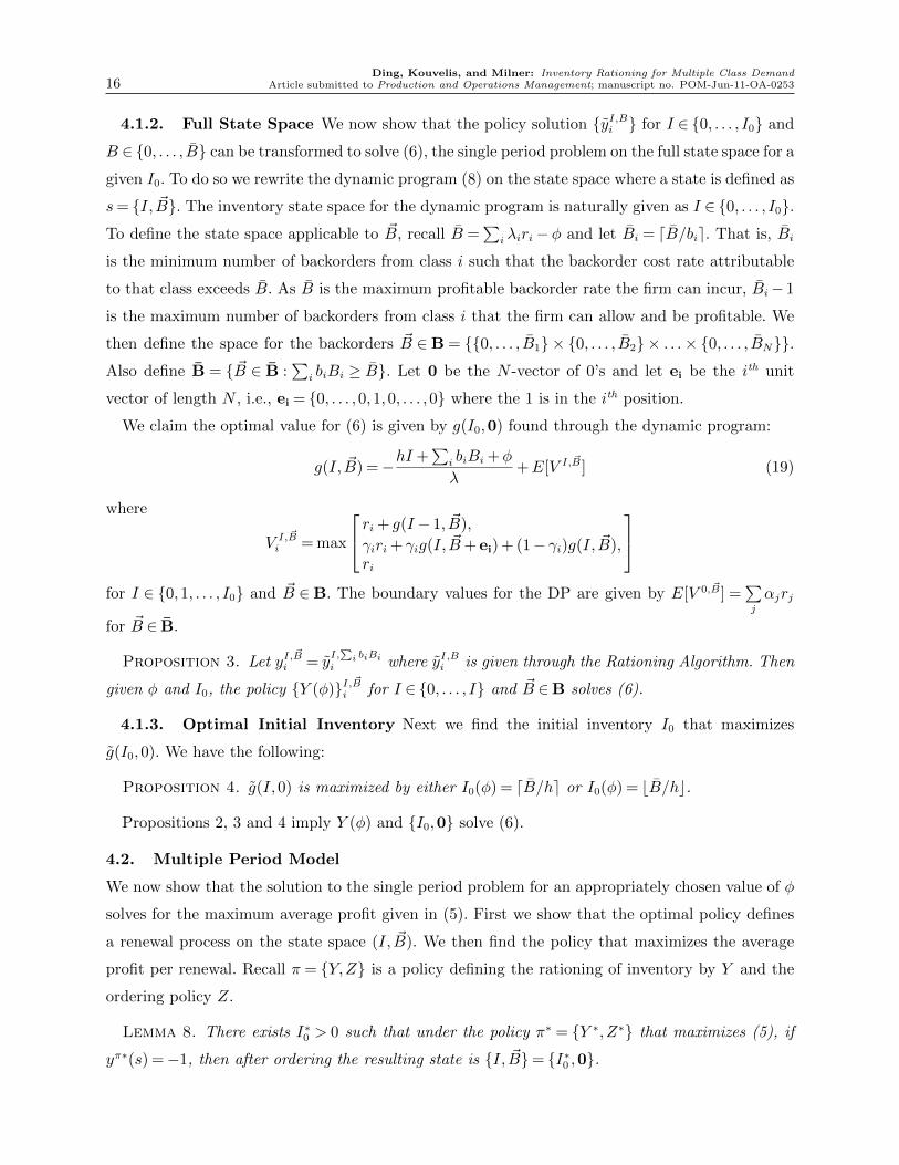
4.1.2. Full State Space We now show that the policy solution yI,Bi for I ∈ 0, . . . , I0 and
B ∈ 0, . . . , B can be transformed to solve (6), the single period problem on the full state space for a
given I0. To do so we rewrite the dynamic program (8) on the state space where a state is defined as
s= I, ~B. The inventory state space for the dynamic program is naturally given as I ∈ 0, . . . , I0.
To define the state space applicable to ~B, recall B =∑
i λiri−φ and let Bi = dB/bie. That is, Bi
is the minimum number of backorders from class i such that the backorder cost rate attributable
to that class exceeds B. As B is the maximum profitable backorder rate the firm can incur, Bi− 1
is the maximum number of backorders from class i that the firm can allow and be profitable. We
then define the space for the backorders ~B ∈B = 0, . . . , B1 × 0, . . . , B2 × . . .× 0, . . . , BN.
Also define B = ~B ∈ B :∑
i biBi ≥ B. Let 0 be the N -vector of 0’s and let ei be the ith unit
vector of length N , i.e., ei = 0, . . . ,0,1,0, . . . ,0 where the 1 is in the ith position.
We claim the optimal value for (6) is given by g(I0,0) found through the dynamic program:
g(I, ~B) =−hI +
∑i biBi +φ
λ+E[V I, ~B] (19)
where
V I, ~Bi = max
ri + g(I − 1, ~B),
γiri + γig(I, ~B+ ei) + (1− γi)g(I, ~B),ri
for I ∈ 0,1, . . . , I0 and ~B ∈B. The boundary values for the DP are given by E[V 0, ~B] =
∑j
αjrj
for ~B ∈ B.
Proposition 3. Let yI,~B
i = yI,∑i biBi
i where yI,Bi is given through the Rationing Algorithm. Then
given φ and I0, the policy Y (φ)I, ~Bi for I ∈ 0, . . . , I and ~B ∈B solves (6).
4.1.3. Optimal Initial Inventory Next we find the initial inventory I0 that maximizes
g(I0,0). We have the following:
Proposition 4. g(I,0) is maximized by either I0(φ) = dB/he or I0(φ) = bB/hc.
Propositions 2, 3 and 4 imply Y (φ) and I0,0 solve (6).
4.2. Multiple Period Model
We now show that the solution to the single period problem for an appropriately chosen value of φ
solves for the maximum average profit given in (5). First we show that the optimal policy defines
a renewal process on the state space (I, ~B). We then find the policy that maximizes the average
profit per renewal. Recall π = Y,Z is a policy defining the rationing of inventory by Y and the
ordering policy Z.
Lemma 8. There exists I∗0 > 0 such that under the policy π∗ = Y ∗,Z∗ that maximizes (5), if
yπ∗(s) =−1, then after ordering the resulting state is I, ~B= I∗0 ,0.
Ding, Kouvelis, and Milner: Inventory Rationing for Multiple Class DemandArticle submitted to Production and Operations Management; manuscript no. POM-Jun-11-OA-0253 17
Let π(φ) = Y (φ),Z(φ) be the φ-dependent policy for the multiple period model where Y (φ)
is the φ-dependent optimal rationing policy given by the Rationing Algorithm and Z(φ) is the
policy that orders up to the (φ-dependent) I0(φ) given in Proposition 4, and clears all backorders
so that ~B = 0 after ordering. In Step 3 of the Rationing Algorithm, we track for I,B, ΠI,Bi , the
profit-to-go without the φ terms, and T I,Bi , the time-to-go, given a class-i arrival. Then following
policy π(φ) in the multiple period model, starting in state σ= I0(φ),0, the expected profit- and
time-to-go until another order is placed are
Π(φ) =E[ΠI0(φ),0i ]−hI0(φ)/λ and (20)
T (φ) =E[TI0(φ),0i ] + 1/λ (21)
where the expectations are taken over the class of the first arrival. For the single period model
the expected reward less operating cost until closing is given by g(I0(φ),0) = Π(φ)−φT (φ). In the
multiple period model, we have the following:
Lemma 9. The expected reward in each renewal cycle under policy π(φ) starting in state σ =
I0(φ),0 is given by
vπ(φ),σ1 ≡E
uπ(φ),σ1 (x)∑n=1
rπ(φ),σn (x)−
∫ Tπ(φ),σ1 (x)
0
cπ,σt (x)dt−K
= Π(φ)−K.
Together Lemmas 8 and 9 imply
Proposition 5. The average reward under policy π(φ) is
hπ(φ) =Π(φ)−KT (φ)
.
Assuming there is a value of φ inducing a policy π(φ) such that Π(φ) > K, we can find the
optimal policy. That is, we observe
Proposition 6. If there exists φ> 0 such that Π(φ)>K, then there exists a unique φ∗ such that
π(φ∗) ≡ Y ∗, I∗0 = Y (φ∗), I0(φ∗) maximizes the average policy reward given an initial state(as
formally defined in (5)) and φ∗ = hπ(φ∗) is the maximum average profit.
Let φ=∑
i λiri. An ε-optimal policy can be found by bisection search on φ ∈ [0, φ], solving the
Rationing Algorithm for f(φ) = hπ(φ) = (Π(φ)−K)/T (φ) and adjusting φ until |f(φ)− φ|< ε for
some small ε > 0. Because I0 and B are both O(φ), there are O(φ2) states (I,B). From Step 1
of the Algorithm, for each state (I,B), we need to determine and sort the βi, for i ∈ N taking
Ding, Kouvelis, and Milner: Inventory Rationing for Multiple Class Demand18 Article submitted to Production and Operations Management; manuscript no. POM-Jun-11-OA-0253
O(N logN) time. The remaining steps take O(N) time. So the total time required for each value
of φ is O(φ2N logN). Thus determining the optimal policy requires O(φ2N logN log (φ/ε)) time.
Note that the state space for the problem tracking the number of backorders from all classes is
O(φN+1).
We can make several comments regarding the optimal policy. By allowing the firm to choose
which customer classes to delay (as opposed to a first-come/first-served policy), the average profit
per unit time, φ∗, is greater than what it would be without rationing. We then observe this has
the effect of decreasing the purchase quantity, I∗0 ≈ (φ−φ∗)/h. Similarly, this also has the effect of
lowering the bound for the point where a new order is placed because θ∗i ≈ φ−φ∗−γibi−(1−γi)riλ.
Thus, the flexibility provided by the ability to ration inventory allows the firm to order less inventory
with fewer backlogs.
5. Comparison to Static and Single Class Policies
In this section we consider two questions: First, in what instances is it valuable to allocate inventory
through a dynamic policy rather than a static one? Second, what is the value of considering the
customer class of an arrival when determining if the firm should place a reorder? These questions are
at the heart of the current paper as they address the need to track the current inventory, backorder
cost rate, and class of each arriving customer as is done in the Rationing Algorithm. To address
these questions we compare the optimal policy and its profit rate to two static heuristics. These
are based on the results of the problem set in a deterministic EOQ-like environment presented in
Ding et al. (2007). We emphasize that we use these heuristics to gain insight into the properties of
the optimal solution and not as a solution technique in and of themselves.
Ding et al. (2007) determine an optimal policy defined by a base stock SDet, a reorder time TDet,
and run-out times tDeti for each class i, prior to which demand from class i is served and after which
it is either backordered or lost, depending on γi. Let yDetit = 1 if t < tDeti and 0 otherwise, and let φDet
be the average profit rate given in the deterministic setting. Then by definition, SDet =∑
j λjtDetj .
The heuristics we consider transform the deterministic policy into a feasible policy for prob-
lem (7). Without loss of generality assume tDet1 > tDet2 > · · ·> tDetN , i.e., class-1 is the highest class.
Suppose we serve class-i customers from stock as long as the inventory on hand exceeds Si−1. That
is, let Si be the protected stock for classes i and higher. Then Si =∑i
j=1 λj(tDetj − tDeti+1) noting
SN = SDet by letting tDetN+1 = 0. Also define S0 = 0.
In the two deterministic heuristics, a reorder is placed when the total effective backorder cost
rate exceeds some deterministic threshold. The total effective backorder rate, Bt is the sum of the
backorder cost rates, bi, for all delayed customers arriving by time t who agree to wait to be served
Ding, Kouvelis, and Milner: Inventory Rationing for Multiple Class DemandArticle submitted to Production and Operations Management; manuscript no. POM-Jun-11-OA-0253 19
from a reorder. The heuristics differ only on the definition of the threshold. From Proposition 1,
we know the optimal threshold
θi ≥ B− γibi− (1− γi)riλ=∑i
(λiri−φ)− γibi− (1− γi)riλ.
Suppose we substitute in φDet for φ and define
θDeti ≡∑i
(λiri−φDet)− γibi− (1− γi)riλ.
The Class-Dependent Heuristic (CDH) serves class-i customers from stock as long as the inventory
on hand exceeds Si−1 and places a reorder to bring the inventory up to SDet when a class-i customer
arrives and the total effective backorder cost rate, Bt ≥ θDeti . The policy is static in that the cut-off
values Si are not determined dynamically and the reorder threshold, θDeti , is defined by the static
profit rate.
To address our second question, we consider a Class-Independent Heuristic (CIH). Under this
policy, a reorder is placed when inventory is depleted and the backorder cost rate is sufficiently
high, exceeding θDet ≡∑
i λi∫ TDet
0(1− yDetit )(γibi)dt. For the CIH we place a reorder to bring the
inventory up to SDet when no inventory remains and the actual total effective backorder cost,
Bt ≥ θDet. Thus, the reorder decision is made independent of the arriving customer class.
We illustrate the difference between the optimal policy and those given by the heuristics through
a two-customer class example. We let r1 = 15, r2 = 10, b1 = 1.5, b2 = 1.0, γ2 = 1, h = 0.5, and
K = 1000. For Test Case-1 we let λ1 = λ2 = 10, and vary the percentage of class-1 customers willing
to wait, γ1, from 0 to 100%. In Test Case-2, we let γ1 = 0 and, while maintaining λ1 + λ2 = 20,
vary λ1 from 0 to 20, illustrating the effect of the customer mix. For each test case we simulated
100,000 time periods.
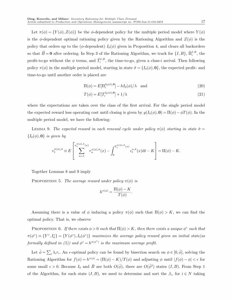
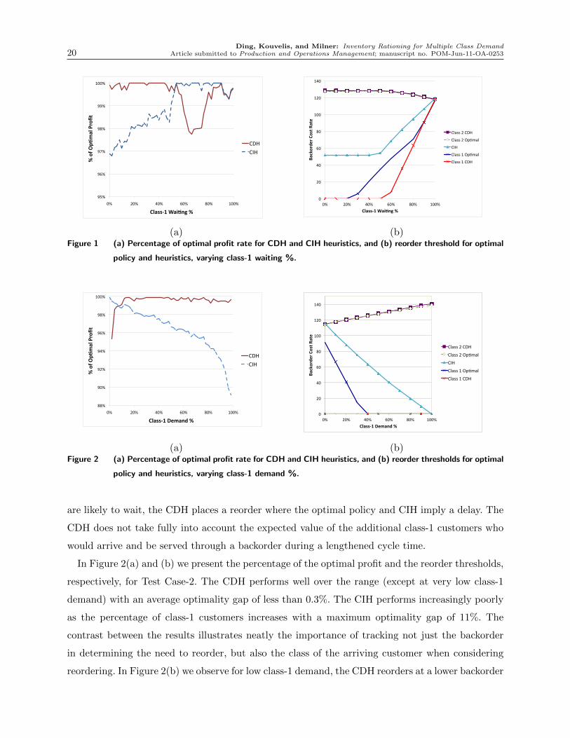
In Figure 1(a) we present the percentage of the optimal average profit achieved by each heuristic
as a function of the percentage of class-1 customers waiting as given by Test Case-1. We observe
that the two heuristics perform adequately, though on differing segments (the optimality gap of
the CDH is about 0.5% on average; the CIH, 1.0%). The performance can be traced to how each
heuristic treats reorders, in particular, those triggered or not by the arrival of a high-value class-1
customer. In Figure 1(b) we present the reorder thresholds as the percentage of class-1 customers
waiting varies for both CIH and CDH heuristics and the optimal policy. We observe the CIH reorder
threshold lies between the optimal ones for classes-1 and -2. When class-1 customers are unlikely to
wait, the reorder point for the CIH is significantly higher than that of the optimal class-1 threshold.
Thus, the CIH does not place an order for a class-1 customer, as it does not differentiate between
classes. In doing so it delays orders and incurs lost revenue from class-1. When class-1 customers
Ding, Kouvelis, and Milner: Inventory Rationing for Multiple Class Demand20 Article submitted to Production and Operations Management; manuscript no. POM-Jun-11-OA-0253
95%
96%
97%
98%
99%
100%
0% 20% 40% 60% 80% 100%
%ofO
p'malProfit
Class‐1Wai'ng%
CDH
CIH
(a)
0
20
40
60
80
100
120
140
0% 20% 40% 60% 80% 100%
Backorde
r Cost R
ate
Class-‐1 Wai3ng %
Class 2 CDH
Class 2 Op1mal
CIH
Class 1 Op1mal
Class 1 CDH
(b)Figure 1 (a) Percentage of optimal profit rate for CDH and CIH heuristics, and (b) reorder threshold for optimal
policy and heuristics, varying class-1 waiting %.
88%
90%
92%
94%
96%
98%
100%
0% 20% 40% 60% 80% 100%
%ofO
p'malProfit
Class‐1Demand%
CDH
CIH
(a)
0
20
40
60
80
100
120
140
0% 20% 40% 60% 80% 100%
Backorde
r Cost R
ate
Class-‐1 Demand %
Class 2 CDH
Class 2 Op1mal
CIH
Class 1 Op1mal
Class 1 CDH
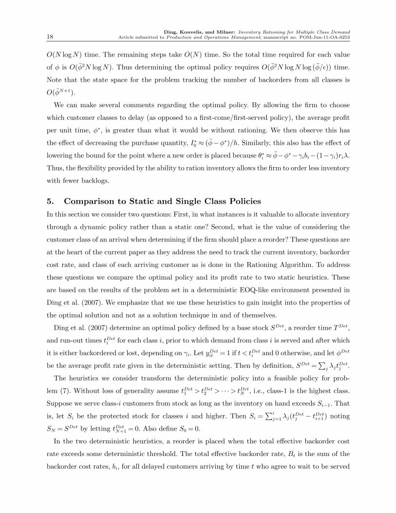
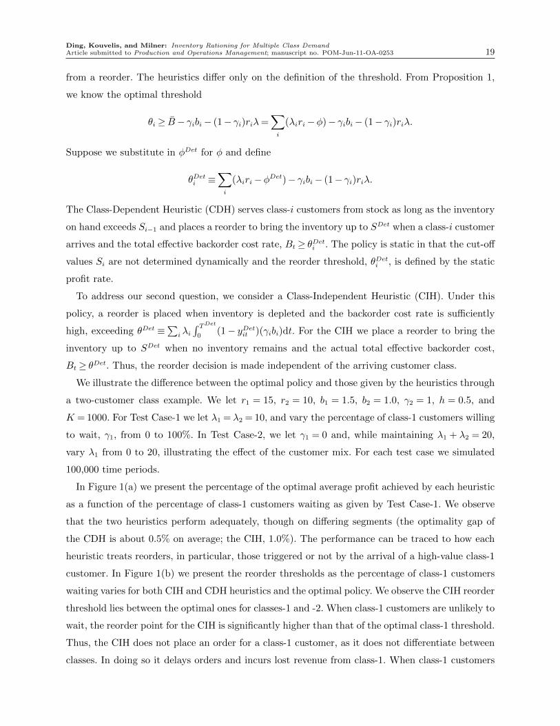
(b)Figure 2 (a) Percentage of optimal profit rate for CDH and CIH heuristics, and (b) reorder thresholds for optimal
policy and heuristics, varying class-1 demand %.
are likely to wait, the CDH places a reorder where the optimal policy and CIH imply a delay. The
CDH does not take fully into account the expected value of the additional class-1 customers who
would arrive and be served through a backorder during a lengthened cycle time.
In Figure 2(a) and (b) we present the percentage of the optimal profit and the reorder thresholds,
respectively, for Test Case-2. The CDH performs well over the range (except at very low class-1
demand) with an average optimality gap of less than 0.3%. The CIH performs increasingly poorly
as the percentage of class-1 customers increases with a maximum optimality gap of 11%. The
contrast between the results illustrates neatly the importance of tracking not just the backorder
in determining the need to reorder, but also the class of the arriving customer when considering
reordering. In Figure 2(b) we observe for low class-1 demand, the CDH reorders at a lower backorder
Ding, Kouvelis, and Milner: Inventory Rationing for Multiple Class DemandArticle submitted to Production and Operations Management; manuscript no. POM-Jun-11-OA-0253 21
cost than the optimal policy, reducing profitability. As the class-1 demand increases, the CIH
approaches the class-1 optimal policy, but differs greatly from the class-2 optimal policy. This
incurs high setup costs when class-2 customers arrive and trigger setups rather than being placed
on backorder.
Taken together, the two test cases show that the optimal policy demonstrates three qualities
held by the static heuristic: (1) It will cut-off provision of supply to the second customer class
prior to cutting off supply to the first; (2) it will reorder sufficient inventory to fill the demand
of any waiting customers plus enough to last through the next cycle; and (3) it will place an
order approximately when the backorder cost rate plus the cost of losing the current customer
exceeds the average operating cost rate. Further, because the ordering policy of the CDH is based
on the expected profit rate, φDet, the optimal profit rate may be close to the profit rate from the
deterministic case and thus φDet may provide a very good starting point for the search for the
On the other hand, we observe that the static CDH can lead to significant losses in two cases:
when class-1 customers are more likely to wait for a delayed service and when class-1 customers
are relatively rare. In both cases, the firm should trade-off the lost revenue from customers that do
not wait with the savings in setup costs and the revenue gains from those customers (class-1 and
-2) that do wait for delayed service. This illustrates the need to dynamically take the future value
of customers arriving during an order cycle into account when making costly reorder decisions.
6. Model Extensions
In our model formulation we let ri represent the revenue per unit. With no change in the model,
ri can also represent the margin per unit (the revenue less cost per unit). In addition, if there is
a per unit lost sale penalty, then ri can represent the margin per unit plus the lost sale penalty.
These all follow from standard inventory theory noting ri represents the relative benefit of serving
a customer over delaying or losing the customer. Also in the model we assume that the firm incurs
a cost per unit time, bi, for backlogging a class-i customer. We can extend the model to also include
a fixed cost per customer backlogged, independent of time. That is, letting di be the fixed cost of
delaying a customer (assuming they accept the delay), the expected costs of delaying a customer is
γi(ri+di)+(hI+B+γibi+φ)/λ+γig(I,B+bi)+(1−γ)g(I,B). All of the lemmas and propositions
hold for this extension, the only change being the lower bound given in Proposition 1 decreases by
γidiλ, i.e., θi ≥ B− γi(bi + diλ)− (1− γi)riλ.
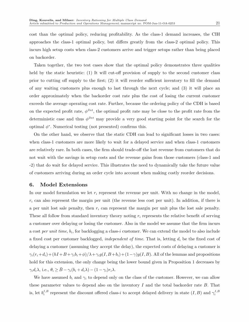
We have assumed bi and γi to depend only on the class of the customer. However, we can allow
these parameter values to depend also on the inventory I and the total backorder rate B. That
is, let bI,Bi represent the discount offered class-i to accept delayed delivery in state (I,B) and γI,Bi
Ding, Kouvelis, and Milner: Inventory Rationing for Multiple Class Demand22 Article submitted to Production and Operations Management; manuscript no. POM-Jun-11-OA-0253
represent the likelihood the offer is accepted. Then all of the theoretical results developed in the
model can be shown to hold for this case as well. Observe that the firm could announce the expected
time until a delayed customer is served, T I,Bi so that γI,Bi could depend on both the discount and
the expected time until a delayed customer is served. Alternatively, the firm could use the values of
T I′,B′
j for future states I ′,B′ and the dynamic program solution to estimate a time until service
that occurs with some high likelihood. Thus customers can make their decision to accept or balk
based on the discount bi and information regarding delay. (See Armony et al. (2009) who discuss
such announcements and customer balking in call center contexts.)
Further, we can allow the firm to optimize over bI,Bi . From Lemma 6 we observe that the expected
total value-to-go for all classes in state (I,B) in the objective function in (12a) is given by
Total ValueI,B ≡∑i∈J
(1− γI,Bi )
(βI,Bi +
∑j∈J β
I,Bj αj(1− γI,Bj )
1−∑
j∈J αj(1− γI,Bj )
)+∑i∈N
Servei
where βI,Bi and J are given in the statement of Lemma 6. Then if γI,Bi were a function of bI,Bi ,
the firm could solve the nonlinear program maxbI,B Total ValueI,B for each state (I,B) where
bI,B = bI,B1 , . . . , bI,BN . A difficulty in solving this nonlinear program is that the set J depends on
βI,Bi . However, we can address the problem using an approximate dynamic programming approach
presented in Appendix B.
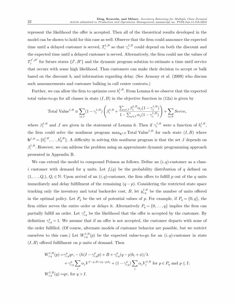
We can extend the model to compound Poisson as follows. Define an (i, q)-customer as a class-
i customer with demand for q units. Let fi(q) be the probability distribution of q defined on
(1, . . . ,Qi), Qi ∈N. Upon arrival of an (i, q)-customer, the firm offers to fulfill p out of the q units
immediately and delay fulfillment of the remaining (q− p). Considering the restricted state space
tracking only the inventory and total backorder cost, B, let yI,Bi,q be the number of units offered
in the optimal policy. Let Pq be the set of potential values of p. For example, if Pq = 0, q, the
firm either serves the entire order or delays it. Alternatively Pq = 0, . . . , q implies the firm can
partially fulfill an order. Let γpi,q be the likelihood that the offer is accepted by the customer. By
definition γqi,q = 1. We assume that if an offer is not accepted, the customer departs with none of
the order fulfilled. (Of course, alternate models of customer behavior are possible, but we restrict
ourselves to this case.) Let W I,Bi,q (p) be the expected value-to-go for an (i, q)-customer in state
(I,B) offered fulfillment on p units of demand. Then
Ding, Kouvelis, and Milner: Inventory Rationing for Multiple Class DemandArticle submitted to Production and Operations Management; manuscript no. POM-Jun-11-OA-0253 23
Then we can replace the linear program (12a)–(12c) with
min∑i,q
V I,Bi,q (22a)
s.t.
V I,Bi,q ≥W
I,Bi,q (p) for all p∈ Pq, q ∈Qi, i∈N (22b)
V I,Bi =
Qi∑q=1
fi(q)VI,Bi,q for all i∈N (22c)
The solution to (22a)–(22c) provides the optimal values of yI,Bi,q . Step 2 of the Rationing Algorithm
must be slightly altered so yI,Bi,q = p if V I,Bi,q = W I,B
i,q (p), and yI,Bi,q = −1 (a reorder is placed) if
V I,Bi,q =W I,B
i,q (q) for q > I. Step 3 of the algorithm must be altered so that the values of ΠI,Bi,q and
T I,Bi,q for serving p out of q units solve the simultaneous linear equations:
ΠI,Bi,q = γpi,qqri−
(h(I − γpi,qp) +B+ γpi,q(q− p)bi
)/λ+ γpi,q
∑j
αjΠI−p,B+(q−p)bij + (1− γpi,q)
∑j
αjΠI,Bj ,
T I,Bi,q = 1/λ+ γpi,q∑j
αjTI−p,B+(q−p)bij + (1− γpi,q)
∑j
αjTI,Bj , for i∈N such that yI,Bi ≥ 0; and
ΠI,Bi,q = qri, T
I,Bi,q = 0 for yI,Bi =−1.
We note the solution given in Lemma 6 still holds. Observe that W I,Bi,q (p) depends on V I,B
i similar
to how DelayI,Bi does. In the compound Poisson case, V I,Bi is given by the linking constraint (22c).
The structure of (22a)–(22c) is the same as (12a)–(12c). This is shown by substituting (22c) into
(22b) and then noting the terms W I,Bi,q (q) give the value-to-go of serving an order, or reordering
if q > I. By defining βI,Bi,q analogous to that in Lemma 6 and ordering them, we can efficiently
determine V I,Bi,q . Letting Q be the maximum value of Qi over all i ∈N , we can solve (22a)–(22c)
in O(NQ logNQ) steps.
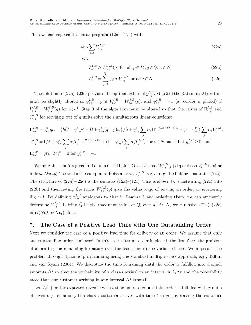
7. The Case of a Positive Lead Time with One Outstanding Order
Next we consider the case of a positive lead time for delivery of an order. We assume that only
one outstanding order is allowed. In this case, after an order is placed, the firm faces the problem
of allocating the remaining inventory over the lead time to the various classes. We approach the
problem through dynamic programming using the standard multiple class approach, e.g., Talluri
and van Ryzin (2004). We discretize the time remaining until the order is fulfilled into a small
amounts ∆t so that the probability of a class-i arrival in an interval is λi∆t and the probability
more than one customer arriving in any interval ∆t is small.
Let Vt(x) be the expected revenue with t time units to go until the order is fulfilled with x units
of inventory remaining. If a class-i customer arrives with time t to go, by serving the customer
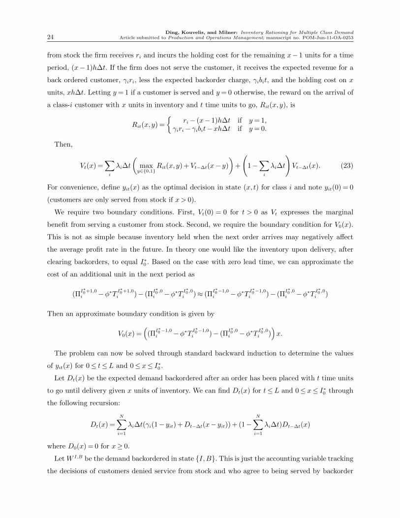
Ding, Kouvelis, and Milner: Inventory Rationing for Multiple Class Demand24 Article submitted to Production and Operations Management; manuscript no. POM-Jun-11-OA-0253
from stock the firm receives ri and incurs the holding cost for the remaining x− 1 units for a time
period, (x− 1)h∆t. If the firm does not serve the customer, it receives the expected revenue for a
back ordered customer, γiri, less the expected backorder charge, γibit, and the holding cost on x
units, xh∆t. Letting y= 1 if a customer is served and y= 0 otherwise, the reward on the arrival of
a class-i customer with x units in inventory and t time units to go, Rit(x, y), is
Rit(x, y) =
ri− (x− 1)h∆t if y= 1,
γiri− γibit−xh∆t if y= 0.
Then,
Vt(x) =∑i
λi∆t
(maxy∈0,1
Rit(x, y) +Vt−∆t(x− y)
)+
(1−
∑i
λi∆t
)Vt−∆t(x). (23)
For convenience, define yit(x) as the optimal decision in state (x, t) for class i and note yit(0) = 0
(customers are only served from stock if x> 0).
We require two boundary conditions. First, Vt(0) = 0 for t > 0 as Vt expresses the marginal
benefit from serving a customer from stock. Second, we require the boundary condition for V0(x).
This is not as simple because inventory held when the next order arrives may negatively affect
the average profit rate in the future. In theory one would like the inventory upon delivery, after
clearing backorders, to equal I∗0 . Based on the case with zero lead time, we can approximate the
cost of an additional unit in the next period as
(ΠI∗0+1,0i −φ∗T I
∗0+1,0i )− (Π
I∗0 ,0i −φ∗T I
∗0 ,0i )≈ (Π
I∗0−1,0i −φ∗T I
∗0−1,0i )− (Π
I∗0 ,0i −φ∗T I
∗0 ,0i )
Then an approximate boundary condition is given by
V0(x) =(
(ΠI∗0−1,0i −φ∗T I
∗0−1,0i )− (Π
I∗0 ,0i −φ∗T I
∗0 ,0i )
)x.
The problem can now be solved through standard backward induction to determine the values
of yit(x) for 0≤ t≤L and 0≤ x≤ I∗0 .
Let Dt(x) be the expected demand backordered after an order has been placed with t time units
to go until delivery given x units of inventory. We can find Dt(x) for t≤L and 0≤ x≤ I∗0 through
the following recursion:
Dt(x) =N∑i=1
λi∆t(γi(1− yit) +Dt−∆t(x− yit)) + (1−N∑i=1
λi∆t)Dt−∆t(x)
where D0(x) = 0 for x≥ 0.
Let W I,B be the demand backordered in state I,B. This is just the accounting variable tracking
the decisions of customers denied service from stock and who agree to being served by backorder
Ding, Kouvelis, and Milner: Inventory Rationing for Multiple Class DemandArticle submitted to Production and Operations Management; manuscript no. POM-Jun-11-OA-0253 25
prior to placing the order with L time units to go. Then at the time an order is placed, the order
quantity required to bring the expected order up to I∗0 is
QI,B = I∗0 +W I,B +DL(I). (24)
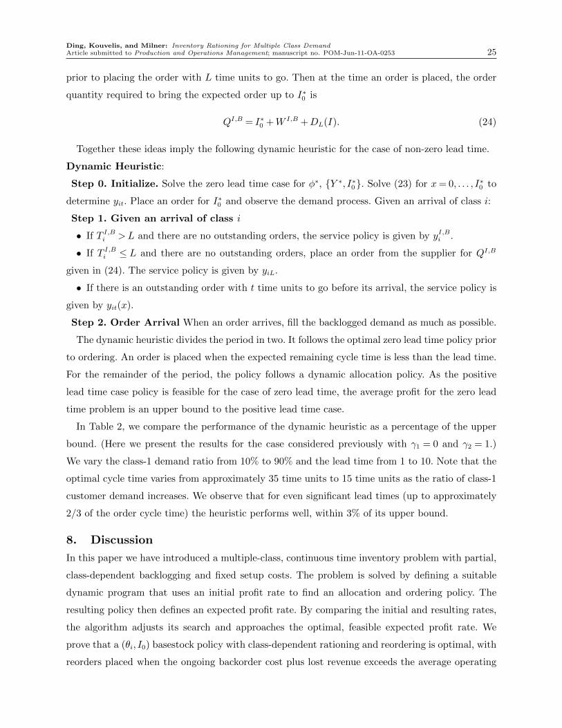
Together these ideas imply the following dynamic heuristic for the case of non-zero lead time.
Dynamic Heuristic:
Step 0. Initialize. Solve the zero lead time case for φ∗, Y ∗, I∗0. Solve (23) for x= 0, . . . , I∗0 to
determine yit. Place an order for I∗0 and observe the demand process. Given an arrival of class i:
Step 1. Given an arrival of class i
• If T I,Bi >L and there are no outstanding orders, the service policy is given by yI,Bi .
• If T I,Bi ≤ L and there are no outstanding orders, place an order from the supplier for QI,B
given in (24). The service policy is given by yiL.
• If there is an outstanding order with t time units to go before its arrival, the service policy is
given by yit(x).
Step 2. Order Arrival When an order arrives, fill the backlogged demand as much as possible.
The dynamic heuristic divides the period in two. It follows the optimal zero lead time policy prior
to ordering. An order is placed when the expected remaining cycle time is less than the lead time.
For the remainder of the period, the policy follows a dynamic allocation policy. As the positive
lead time case policy is feasible for the case of zero lead time, the average profit for the zero lead
time problem is an upper bound to the positive lead time case.
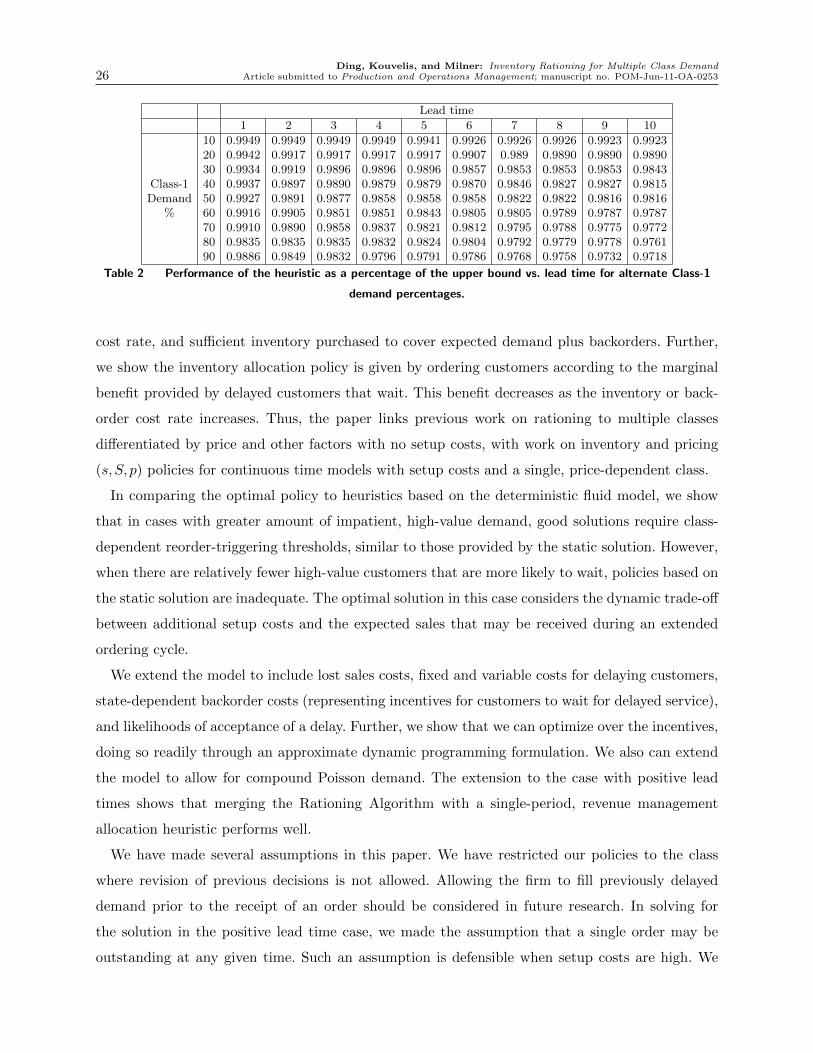
In Table 2, we compare the performance of the dynamic heuristic as a percentage of the upper
bound. (Here we present the results for the case considered previously with γ1 = 0 and γ2 = 1.)
We vary the class-1 demand ratio from 10% to 90% and the lead time from 1 to 10. Note that the
optimal cycle time varies from approximately 35 time units to 15 time units as the ratio of class-1
customer demand increases. We observe that for even significant lead times (up to approximately
2/3 of the order cycle time) the heuristic performs well, within 3% of its upper bound.
8. Discussion
In this paper we have introduced a multiple-class, continuous time inventory problem with partial,
class-dependent backlogging and fixed setup costs. The problem is solved by defining a suitable
dynamic program that uses an initial profit rate to find an allocation and ordering policy. The
resulting policy then defines an expected profit rate. By comparing the initial and resulting rates,
the algorithm adjusts its search and approaches the optimal, feasible expected profit rate. We
prove that a (θi, I0) basestock policy with class-dependent rationing and reordering is optimal, with
reorders placed when the ongoing backorder cost plus lost revenue exceeds the average operating
Ding, Kouvelis, and Milner: Inventory Rationing for Multiple Class Demand26 Article submitted to Production and Operations Management; manuscript no. POM-Jun-11-OA-0253
Table 2 Performance of the heuristic as a percentage of the upper bound vs. lead time for alternate Class-1
demand percentages.
cost rate, and sufficient inventory purchased to cover expected demand plus backorders. Further,
we show the inventory allocation policy is given by ordering customers according to the marginal
benefit provided by delayed customers that wait. This benefit decreases as the inventory or back-
order cost rate increases. Thus, the paper links previous work on rationing to multiple classes
differentiated by price and other factors with no setup costs, with work on inventory and pricing
(s,S, p) policies for continuous time models with setup costs and a single, price-dependent class.
In comparing the optimal policy to heuristics based on the deterministic fluid model, we show
that in cases with greater amount of impatient, high-value demand, good solutions require class-
dependent reorder-triggering thresholds, similar to those provided by the static solution. However,
when there are relatively fewer high-value customers that are more likely to wait, policies based on
the static solution are inadequate. The optimal solution in this case considers the dynamic trade-off
between additional setup costs and the expected sales that may be received during an extended
ordering cycle.
We extend the model to include lost sales costs, fixed and variable costs for delaying customers,
state-dependent backorder costs (representing incentives for customers to wait for delayed service),
and likelihoods of acceptance of a delay. Further, we show that we can optimize over the incentives,
doing so readily through an approximate dynamic programming formulation. We also can extend
the model to allow for compound Poisson demand. The extension to the case with positive lead
times shows that merging the Rationing Algorithm with a single-period, revenue management
allocation heuristic performs well.
We have made several assumptions in this paper. We have restricted our policies to the class
where revision of previous decisions is not allowed. Allowing the firm to fill previously delayed
demand prior to the receipt of an order should be considered in future research. In solving for
the solution in the positive lead time case, we made the assumption that a single order may be
outstanding at any given time. Such an assumption is defensible when setup costs are high. We
Ding, Kouvelis, and Milner: Inventory Rationing for Multiple Class DemandArticle submitted to Production and Operations Management; manuscript no. POM-Jun-11-OA-0253 27
note that the heuristic approach is still very good even as the lead time approaches the cycle time.
Extending the problem to allowing multiple outstanding orders would be useful.
References
Armony, M., N. Shimkin, W. Whitt. 2009. The impact of delay announcements in many-server queues with
abandonment. Operations Research 57(1) 66–81.
Arslan, H., S. C. Graves, T. Roemer. 2007. A single-product inventory model for multiple demand classes.
Management Science 53(9) 1486–1499.
Ayvaz, N., W. T. Huh. 2010. Allocation of hospital beds to different classes of patients: a dynamic-
programming approach. Journal of Revenue and Pricing Management 9 386–398.
Benjaafar, S., M. Elhafsi. 2006. Production and inventory control of a single product assemble-to-order
system with multiple customer classes. Management Science 52(12) 1896–1912.
Benjaafar, S., J.-P. Gayon, S. Tepe. 2010. Optimal control of a production-inventory system with customer
impatience. Operations Research Letters 38(4) 267–272.
Chen, X., D. Simchi-Levi. 2004a. Coordinating inventory control and pricing strategies: The continuous
review model. Operations Research Letters 34 323–332.
Chen, X., D. Simchi-Levi. 2004b. Coordinating inventory control and pricing strategies with random demand
and fixed ordering cost: The finite horizon case. Mathematics of Operations Research 29(3) 698–723.
Chen, X., D. Simchi-Levi. 2004c. Coordinating inventory control and pricing strategies with random demand
and fixed ordering cost: The infinite horizon case. Operations Research 52(6) 887–896.
Dekker, R., M. J. Kleijn, P. J. de Rooij. 1998. A spare parts stocking system based on equipment criticality.
International Journal of Production Economics 56-57 69–77.
Deshpande, V., M. A. Cohen, K. Donohue. 2003. A threshold inventory rationing policy for service-
Ding, Q., P. Kouvelis, J. Milner. 2006. Dynamic pricing through customer discounts for optimizing multi-class
customers demand fulfillment. Operations Research 54(1) 169–183.
Ding, Q., P. Kouvelis, J. Milner. 2007. Dynamic pricing for multiple class deterministic demand fulfillment.
IIE Transactions 39(11) 997–1013.
Feng, Y., F. Y. Chen. 2003. Joint pricing and inventory control with setup costs and demand uncertainty.
Working paper, Department of Systems Engineering and Engineering Management, The Chinese Univ.
of Hong Kong.
Frank, K. C., R. Q. Zhang, I. Duenyas. 2003. Optimal policies for inventory systems with priority demand
classes. Operations Research 51(6) 993–1002.
Ding, Kouvelis, and Milner: Inventory Rationing for Multiple Class Demand28 Article submitted to Production and Operations Management; manuscript no. POM-Jun-11-OA-0253
Ha, A. Y. 1997. Inventory rationing in a make-to-stock production system with several demand classes and
lost sales. Management Science 43(8) 1093–1103.
Huh, W. T., G. Janakiraman. 2008. (s, S) optimality in joint inventory-pricing control: An alternate approach.
Operations Research 56(3) 783–790.
Kleijn, M. J., R. Dekker. 1999. An overview of inventory systems with several demand classes. New Trends
in Distribution Logistics, Lecture Notes in Economics and Mathematical Systems, vol. 480. Springer,
253–265.
Melchiors, P., R. Dekker, M. J. Kleijn. 2000. Inventory rationing in an (s, q) inventory model with lost sales
and two demand classes. Journal of the Operational Research Society 51(1) 111–122.
Moon, I., S. Kang. 1998. Rationing policies for some inventory system. The Journal of the Operational
Research Society 49(5) 509–518.
Nahmias, S., W. S. Demmy. 1981. Operating characteristics of an inventory system with rationing. Man-
agement Science 27 1236–1245.
Ross, S. 1983. Stochastic Processes. Wiley, New York.
Scarf, H. 1960. The optimality of (s, S) policies in dynamic inventory problem. K. Arrow, S. Karlin, P. Suppes,
eds., Mathematical Models in Social Sciences. Stanford University Press.
Song, Y., S. Ray, T. Boyaci. 2009. Optimal dynamic joint inventory-pricing control for multiplicative demand
with fixed order costs and lost sales. Operations Research 57(1) 245–250.
Talluri, K., G. van Ryzin. 2004. The Theory and Practice of Revenue Management . Kluwer, Norwell,
Massachusetts.
Topkis, D. M. 1968. Optimal ordering and rationing policies in a nonstationary dynamic inventory model
with n demand classes. Management Science 15 160–176.
Zheng, Y.-S. 1991. A simple proof for optimality of (s, S) policies in infinite-horizon inventory systems.
Journal of Applied Probability 28(4) 802–810.
Ding, Kouvelis, and Milner: Inventory Rationing for Multiple Class DemandArticle submitted to Production and Operations Management; manuscript no. POM-Jun-11-OA-0253 1
Appendix A - Proofs
Proof of Lemma 1 Let ωI,Bi ∈ Ω represent the optimal policy followed from an arrival epoch
from class i in state (I,B) onward and let ΠI,B−1i (ωI,Bi ) and T I,B−1
i (ωI,Bi ) be the profit to go
and time to order, respectively, if policy ωI,Bi is employed in state (I,B − 1) for class i. Observe
T I,B−1i (ωI,Bi ) = T I,Bi (ωI,Bi )≡ T I,Bi as the same policy is followed. Also, ΠI,B−1
i (ωI,Bi ) = ΠI,Bi + T I,Bi
as the additional backlogging rate unit is carried for T I,Bi time units. Therefore
V I,B−1i − V I,B
i ≥ (ΠI,B−1i (ωI,Bi )−φT I,B−1
i (ωI,Bi ))− (ΠI,Bi −φT I,Bi )
= (ΠI,Bi + T I,Bi −φT I,Bi )− (ΠI,B
i −φT I,Bi )
= T I,Bi ≥ 0.
Proof of Lemma 2 Consider the base case with no inventory, I = 0.
By definition V 0,Bi = max[ri, V
0,Bi,y=0]. Now,
V 0,Bi,y=0 = γiri− 1/λ
(B+ γibi +φ−
(γi∑j
λj(V0,B+bij ) + (1− γi)
∑j
λj(V0,Bj )
) )
≤ ri− 1/λ
(∑j
λjrj + γibi−
(γi∑j
λj(V0,B+bij ) + (1− γi)
∑j
λj(V0,Bj )
) )≤ ri− γibi/λ+ 1/λ(
∑j
λj(V0,Bj − rj)).
The first inequality holds because, by the Lemma’s assumption, B > B, γi < 1, and by definition∑j λjrj = B+φ. The second holds because V 0,B+bi
j ≤ V 0,Bj as any policy optimizing the case with
backorder cost B+ bi is feasible and at lower cost when the backorder cost is B. Thus we have
V 0,Bi,y=0− ri ≤−γibi/λ+
1
λ
(∑j
λj(V0,Bj − rj)
).
Suppose for some set Ψ⊆N , y0,Bj = 0 for j ∈Ψ, and y0,B
j =−1 for j /∈Ψ. Then
∑j∈Ψ
λj(V0,Bj,y=0− rj)≤−
∑j∈Ψ λjγjbj
λ+
∑j∈Ψ λj
λ
∑j
λj(V0,Bj − rj). (25)
Observe that
∑j
λj(V0,Bj − rj) =
∑j∈Ψ
λj(V0,Bj,y=0− rj) +
∑j 6∈Ψ
λj(V0,Bj,y=−1− rj)
=∑j∈Ψ
λj(V0,Bj,y=0− rj) (26)
Ding, Kouvelis, and Milner: Inventory Rationing for Multiple Class Demand2 Article submitted to Production and Operations Management; manuscript no. POM-Jun-11-OA-0253
because for j /∈Ψ, Π0,Bj,y=−1 = rj and T 0,B
j,y=−1 = 0. Therefore substituting (26) into (25) and rearrang-
ing terms we have ∑j 6∈Ψ λj
λ
∑j
λj(V0,Bj − rj)≤−
∑j∈Ψ λjγjbj
λ.
Since the l.h.s. of the inequality is non-negative we have a contradiction. Therefore y0,Bi =−1 for
all i.
Induction: Now assume for some I > 0, V I′−1,Bi = ri for all i and I ′ ≤ I − 1. Consider an arrival
from class i in state (I,B). Observe
V I,Bi,y=1− V
I,Bi,y=−1 =− 1
λ
(φ+h(I − 1) +B−
∑j
λjVI−1,Bj
)
=− 1
λ
(φ+h(I − 1) +B−
∑j
λjrj
)
≤− 1
λ
(φ+
∑j
λjrj −φ−∑j
λjrj
)= 0,
where the second equality holds by the induction assumption and the inequality holds as B ≥ B ≡∑j λjrj −φ. Therefore serving the demand from inventory is suboptimal for all I.
Let Ψ = i such that yI,Bi = 0 and assume w.l.o.g. Ψ = 1, . . . , k for some k≤N . Then for i∈Ψ,
V I,Bi,y=0− ri > 0. Observe i∈Ψ,
V I,Bi,y=0− ri = (γi− 1)ri− (hI +B+ γibi +φ)/λ+ γi
∑j
αjVI,B+bij + (1− γi)
∑j
αjVI,Bj
≤ (γi− 1)ri− (B+φ)/λ+∑j
αjVI,Bj
= (γi− 1)ri−∑j
αjrj +∑j∈Ψ
αjVI,Bj,y=0 +
∑j 6∈Ψ
αjrj
= (γi− 1)ri +∑j∈Ψ
αj(VI,Bj,y=0− rj).
where the inequality follows from Lemma 1. Thus we have
(1−αi)(V I,Bi,y=0− ri
)≤ (γi− 1)ri +
∑j∈Ψ,j 6=i
αj(VI,Bj,y=0− rj) (27)
for all i∈Ψ.
Let
A=
∣∣∣∣∣∣∣∣(1−α1) −α2 . . . −αk−α1 (1−α2) . . . −αk
...−α1 −α2 . . . (1−αk)
∣∣∣∣∣∣∣∣ .
Ding, Kouvelis, and Milner: Inventory Rationing for Multiple Class DemandArticle submitted to Production and Operations Management; manuscript no. POM-Jun-11-OA-0253 3
Also, let βi = (γi− 1)ri, and β = [β1, β2, . . . , βk]′. Then (27) implies Ax≤ β where xi = V I,B
i,y=0− ri.
Observe
A−1 =1
1−∑
i∈Ψαi
∣∣∣∣∣∣∣∣∣∣∣∣
(1−
∑j∈Ψ,j 6=1αj
)α2 . . . αk
α1
(1−
∑j∈Ψ,j 6=2αj
). . . αk
...
α1 α2 . . .(
1−∑
j∈Ψ,j 6=k αj
)
∣∣∣∣∣∣∣∣∣∣∣∣A−1 has all positive entries while β < 0. Therefore x=A−1β < 0. Contradiction. Therefore Ψ = ∅
The first inequality holds by definition of g(I − 1,B) and the second by the assumption of the
lemma.
Ding, Kouvelis, and Milner: Inventory Rationing for Multiple Class Demand4 Article submitted to Production and Operations Management; manuscript no. POM-Jun-11-OA-0253
Proof of Lemma 5 If bj ≤ h, then B > B − h(I − 1)− bj ≥ B − hI. Since B ≤ B − h(I − 1)), by
Lemmas 3 and 4, yI,Bi = 1.
If bj >h, from (28), g(I − 1,B)≥ g(I,B) if∑i
αi
(ri−
hI +B+φ
λ
)+∑i
αi(−(1− γi)ri) =E[γiri]−hI +B+φ
λ< 0.
But B + bj > B − h(I − 1) implies E[γiri] − (hI + B + φ)/λ ≤ (bj − h)/λ − E[(1 − γi)ri] < 0 by
assumption.
So
V I,Bj,y=0 = γjrj + γjg(I,B+ bj) + (1− γj)g(I,B)
≤ rj + g(I,B)
≤ rj + g(I − 1,B)
= V I,Bj,y=1.
Proof of Lemma 6 Let β′I,Bi = γiri− (hI+B+γibi+φ)/λ+γi
∑j αjV
I,B+bij . In the following we
suppress the superscripts (I,B). Linear program (12a)–(12c) may be written as
min∑j
Vj
s.t. Vi ≥ β′i + (1− γi)∑j
αjVj for all i∈N
Vi ≥ Servei for all i∈N.
Then letting xi = Vi−Servei and β′′i = β′i−Servei + (1− γi)∑
j αjServej the LP is equivalent to
min∑j
xj
s.t. xi ≥ β′′i + (1− γi)∑j
αjxj for all i∈N
xi ≥ 0 for all i∈N.
Observe, if γi = 1 then in the solution to the LP x∗i = max[0, β′′i ]. Then substituting in x∗i , we can
eliminate the variable xi and the rows corresponding to i. Thus, we proceed assuming without loss
of generality that γi < 1. Letting
A=
∣∣∣∣∣∣∣∣∣1
1−γ1−α1 −α2 . . . −αN−α1
11−γ2−α2 . . . −αN...
−α1 −α2 . . . 11−γN
−αN
∣∣∣∣∣∣∣∣∣
Ding, Kouvelis, and Milner: Inventory Rationing for Multiple Class DemandArticle submitted to Production and Operations Management; manuscript no. POM-Jun-11-OA-0253 5
and βi = β′′i /(1− γi), we can write the LP as
min∑j
xj s.t. Ax≥ β; x≥ 0. (29)
Substituting in the definition of ServeI,Bi from (10) and simplifying gives (13) and (14). Observe
because 0<αi < 1 and 0≤ γi < 1, the diagonal of A is positive and the remaining entries in each
row are negative. Without loss of generality, we assume the βi are ordered as β1 >β2 > ... > βN .
That x= 0 is optimal if β1 < 0 is immediate. For β1 > 0, let ui be the dual variable associated
with row i in the constraint set in (29). Letting U =∑
i ui, the dual of (29) is
max∑i
uiβi
s.t.
(D)1
1− γiui−αiU ≤ 1 for all i∑
i
ui−U = 0
ui ≥ 0 for all i
Dualizing the constraint∑
i ui−U = 0, the Lagragian dual of (D) is
LD= minη
[maxui,U
∑j
(βj − η)uj + ηU
](30)
s.t.
ui ≤ (1 +αiU)(1− γi)
ui ≥ 0
Observe βi − η < 0 implies ui = 0 and βi − η ≥ 0 implies ui = (1 + αiU)(1− γi). Letting J = j :
βj − η≥ 0 the dual is equivalent to
minη
[maxU≥0
∑j∈J
(βj − η)(1 +αjU)(1− γj) + ηU
]. (31)
Because the term inside the brackets is linear in U , in order that the solution be non-trivial, it
must be that the coefficient of U is 0. That is,
∑j∈J
(αj(βj − η)(1− γj)) + η= 0,
or
η=−∑
j∈J βjαj(1− γj)1−
∑j∈J αj(1− γj)
.
Ding, Kouvelis, and Milner: Inventory Rationing for Multiple Class Demand6 Article submitted to Production and Operations Management; manuscript no. POM-Jun-11-OA-0253
Because the elements of J depend on η and change at the points where η= βj, we need to find the
first k <N where
βk+1(1−k∑j=1
αj(1− γj))<−k∑j=1
βjαj(1− γj).
If none exists then k=N . Noting the independence of the function value on U , (30) implies
LD=∑i∈J
(1− γi)(βi− η)
=∑i∈J
(1− γi)
(βi +
∑j∈J βjαj(1− γj)
1−∑
j∈J αj(1− γj)
)
Let xi = (1− γi)(βi +
∑j∈J βjαj(1−γj)
1−∑j∈J αj(1−γj)
)for j ∈ J and xj = 0 for j 6∈ J . Then we find LD =
∑i xi =∑
j∈J xj and Ax≥ β so x is the optimal solution by the Fundamental Duality Theorem for linear
The first inequality holds by definition of V I,Bj and the second by the assumption of the lemma.
Proof of Proposition 1 I0 ≤ dB/he implies B − h(I0 − 1) ≥ B − h(dB/he − 1) > 0. Therefore,
B0 <B− h(I0− 1) and the first customer is either served or delayed. Then considering an arrival
to some state (I,B), I ≥ 1 and B ≤ B−h(I − 1), by Lemma 5, if I ≥ 1 then B ≤ B−h(I − 1) and
therefore, by Lemma 4, yI,Bi ∈ 0,1. Thus by induction, the firm only closes if I = 0. Finally, by
Lemma 7, if I = 0, the firm only closes if B ≥ θi ≥ B− γibi− (1− γi)riλ.
Proof of Proposition 2 From Lemma 2, we only need to consider B ∈ [0, B]. In Step 0, the
initial case (I,B) = (0, B) establishes that the firm is closed with received revenue ri and the
cycle time remaining is 0. This boundary is also established for B < B ≤ B+ maxi bi on I ∈ [0, I0]
to facilitate the dynamic program. Observe in Step 1 for I > 0, ServeI,Bi = V I,Bi,y=1 and for I = 0,
ServeI,Bi = V I,Bi,y=−1 = ri; and DelayI,Bi = V I,B
i,y=0. Then if V I,B is the solution vector to (12a), then
V I,Bi = ServeI,Bi if ServeI,Bi ≥DelayI,Bi and V I,B
i = DelayI,Bi otherwise. Thus (9a) and (9b) are
satisfied. By Lemma 6 this is the unique solution. Noting ServeI,Bi is given as the value for a
Ding, Kouvelis, and Milner: Inventory Rationing for Multiple Class DemandArticle submitted to Production and Operations Management; manuscript no. POM-Jun-11-OA-0253 7
continuing operation if I > 0 and the terminal value if I = 0, then by Proposition 1, Step 2 specifies
the optimal policy for Y (φ). Step 3 determines the auxiliary values ΠI,Bi and T I,Bi . Note V I,B
i =
ΠI,Bi −φT I,Bi . In Step 4 the algorithm iterates, first over B and subsequently over I. Because the
arrivals are independent, the policy given for each state (i, I,B) is optimal, and by Lemma 1 the
optimal policy for (7) is given by Y starting with I = I0 and B = 0.
Proof of Proposition 3 Base: For all ~B ∈ B, E[V 0, ~B] =∑
j αjrj =E[V 0,B] where B =∑
j bjBj.
Induction: Assume E[V I, ~B] =E[V I,B] for I ≤ I ′ and all ~B such that∑
j bjBj ≥B′ for some I ′ and
B′ such that 0≤ I ′ ≤ I0 and 0≤B′ ≤ B, I ′,B′ 6= I0,0. There are two cases. Case 1: Let I = I ′
and B =B′− 1 (for B′ > 0). Consider some ~B such that∑
j bjBj =B. Then letting yI,~B
i = yI,Bi for
all i∈N , we observe
a. If yI,Bi = 1, V I, ~Bi = ri + g(I − 1, ~B)
= ri−h(I−1)+
∑j bjBj+φ
λ+E[V I−1, ~B]
= ri−h(I−1)+
∑j bjBj+φ
λ+E[V I−1,B]
= V I,Bi ;
b. If yI,Bi =−1 V I, ~Bi = ri = V I,B
i ;
c. If yI,Bi = 0,
V I, ~Bi = γiri + γig(I, ~B+ ei) + (1− γi)g(I, ~B)
= γiri + γi
(−hI′+
∑j bjBj+bj+φ
λ+E[V I, ~B+ei ]
)+ (1− γi)
(−hI+
∑j bjBj+φ
λ+E[V I, ~B]
)= γiri− hI′+B′+γibi+φ
λ+ γiE[V I,B+bi ] + (1− γi)E[V I, ~B].
(32)
The solution to the linear equations (32) for all i such that yI,~B
i = 0 must equal the solution to (8)
given in the Rationing Algorithm as all terms are identical to those solving the cases where yI,Bi = 0
(solved through (12b)). Therefore V I, ~Bi = V I,B
i for all ~B such that∑
j bjBj =B.
Case 2: Let I = I ′ + 1 and B = B′ and consider some ~B such that∑
j bjBj = B. Then the same
argument as in (a)–(c) holds. By induction, on B′ and I ′, Y = yI,Bi maximizes V I0,0i .
Proof of Proposition 4 Let I∗ = B/h so I = dI∗e.
For I ≤ I − 1,
g(I,B)≥−(hI +B+φ
λ
)+∑j
αjrj + g(I − 1,B)
≥ g(I − 1,B)
for B ≤ B. Then by Lemma 1, g(I ,0)≥ g(I,B) for 0≤ I ≤ I − 1 and 0≤B ≤ B.
We next show g(I ,0)≥ g(I,B) for I ≥ I and 0≤B ≤ B. To do so we show by induction E[V I,0]≥
E[V I,B] for I ≥ I and 0≤B ≤ B. First, from Lemma 2, for B ≥ B, E[V I+1,B] =∑
iαiri ≤E[V I,0].
Ding, Kouvelis, and Milner: Inventory Rationing for Multiple Class Demand8 Article submitted to Production and Operations Management; manuscript no. POM-Jun-11-OA-0253
Now assume E[V I+1,B] =∑
iαiri ≤ E[V I,0] for B = B′ + 1,B′ + 2, . . . for some B′, 0 ≤ B′ < B.
Therefore, by induction, E[V I+1,0]≤E[V I,0]. Then repeating these arguments, for I = I+ 2, I+ 3,
. . . establishes E[V I+1,B]≤E[V I,0] for I ≥ I and 0≤B ≤ B. Finally observe this implies
g(I ,0) =−
(hI +φ
λ
)+E[V I,0]
≥−
(hI +φ
λ
)+E[V I,B]
≥−(hI +B+φ
λ
)+E[V I,B]
= g(I,B)
for I ≥ I and 0≤B ≤ B.
Proof of Lemma 8 First observe that the state space to consider for any optimal policy is
finite: By definition I ≥ 0 and B ≥ 0. For the expected revenue rate to exceed the holding cost,
hI ≤ d∑
i λirie. For the expected revenue rate to be greater than the backorder cost B ≤ d∑
i λirie.
Therefore there must be at least one set of recurrent states.
For any state s= I, ~B, let I(s) = I and ~B(s) = ~B. Consider a stationary policy πA. For each
sample path x, let sm(x), m = 1, . . ., be the state immediately after the mth reorder. Assume
~B(sm(x)) 6= 0 for some m. That is, if yπA
(xn) =−1 (an order is placed for the nth arrival under x)
and this is the mth order, then the state at the time of the n+1st arrival is sm(x). Now consider the
Ding, Kouvelis, and Milner: Inventory Rationing for Multiple Class DemandArticle submitted to Production and Operations Management; manuscript no. POM-Jun-11-OA-0253 9
path-dependent set of decisions (labeled πB) that makes the same set of decisions as πA for each
arrival, but does so for each order cycle starting with no backorders, but with the same inventory
as sm(x), m= 1, . . .. Therefore, for a given x, πB follows πA until the first order where πB places an
order to state s1 = I(s1(x)),0 instead of I(s1(x)), ~B(sm). Then until the next order we define
the decision as yπB
i,1 (s) = yπA
i (I(s), ~B(s)+ ~B(s1)). Similarly, for the mth order, πB places an order
so the state is sm = I(sm(x)),0 and we let yπB
i,m(s) = yπA
i (I(s), ~B(s) + ~B(sm)) until the m+ 1st
order is placed.
We show that hπB ,σ, the average profit rate under πB starting in state σ, is greater than hπ
A,σ.
First observe for any M > 0, E[T πB ,σ
M ] = E[T πA,σ
M ] as the mth order is placed for the uπA,σM (x)th
arrival for both πA and πB. Let T πA,σ
0 = 0 and ~B(s0) = 0. Because the backorder cost using πB,∑i bi
~Bi(sm), is less than that of πA in the mth order cycle, the total profit until the M th order for
πB is
vπB ,σ
M =EX
uπA,σM
(x)∑n=1
rπA,σn (x)−
M∑m=1
∫ TπA,σm
TπA,σm−1
(cs,π
A,σt (x)−
∑i
bi ~Bi(sm)
)dt−MK
≤EX
uπA,σM
(x)∑n=1
rπA,σn (x)−
M∑m=1
∫ TπA,σm
TπA,σm−1
cs,πA,σ
t (x)dt−MK
= vπ
A,σM
where the inequality is strict if ~B(sm(x)) 6= 0 for some m≤M . Therefore,
hπB ,σ = lim
M→∞
vπB ,σ
M
E[T π
B ,σM (x)
] > limM→∞
vπA,σ
M
E[T π
A,σM (x)
] = hπA,σ.
Thus, πB is a (possibly path-dependent) policy ordering to s′m(x) = Im,0, m= 1, . . . and has a
higher profit rate than that of πA. Let I = Imx∈X,m=1,..., be the set of Im for all paths x and
all m for policy πB, and let K = |Im|. Let Ik be the kth element of I. Then let πk be the average
cost maximizing policy that always orders up to Ik, filling all backorders. Because πB always
orders up to some I ∈ I, hπB
=∑
kwkhπk for some weights wk ≥ 0,
∑wk = 1. But for some k′,
hπk′
= maxk[hπk ] ≥
∑kwkh
πk ≥ hπA and so for any policy πA, there is a dominating policy πk′.
Because πA was chosen arbitrarily, there must exist I∗0 .
Proof of Lemma 9 Consider a sample path x. Recall revenue rπ(φ),σn (x) is received for customers
n = 1 to n = uπ(φ),σ1 (x) customers. By following Y (φ), for the kth customer in a sample path x
where 1≤ k≤ uπ(φ),σ1 (x), if the state upon arrival is I, ~B, rπ(φ),σ
n (x) = ri if yI,Bi = 1 or yI,Bi =−1,
or rπ(φ),σn (x) = γiri if yI,Bi = 0. Letting the initial state be σ = I0(φ),0 and taking expectations
Ding, Kouvelis, and Milner: Inventory Rationing for Multiple Class Demand10 Article submitted to Production and Operations Management; manuscript no. POM-Jun-11-OA-0253
over all sample paths, the expected revenue defined by (2) equals the revenue terms in Π(φ) as
defined by Step 3 of the rationing algorithm and (20).
Similarly, cπ(φ),σt (x), the operating cost (the holding plus backorder cost) depends only on the
state at each time t between 0 and Tπ(φ),σ1 (x), the time of the first order. If under Y (φ), the
system is in state I, ~B from time t1 to t2, 0 ≤ t1 < t2 ≤ T π(φ),σ1 (x), then the cost incurred is
(t2 − t1)(hI +∑
i biBi). Noting that the expected holding cost until the first order is received,
hI0(φ)/λ, is added to E[ΠI0(φ),0i ], and again taking expectations over all sample paths, the operating
cost defined in (3) equals the operating costs in Π(φ) as defined by Step 3 of the rationing algorithm
and (20). Subtracting the ordering cost, K, gives the result.
Proof of Proposition 5 Lemma 8 implies that under policy π(φ), there is a renewal in state
I0(φ),0 and by Lemma 9, the reward between renewals following π(φ) is given by Π(φ)−K.
The expected time between renewals, T (φ), is defined by Step 3 and (21). By the Renewal Reward
Theorem (see, e.g., Ross (1983), 3.6.1), the average reward is independent of the initial state so
that for any initial state σ,
hπ(φ) = limM→∞
vπ,σME [T π,σM (x)]
=Π(φ)−KT (φ)
.
Proof of Proposition 6 Let φ=∑
i λiri. Let K(φ) = Π(φ)−φT (φ). Observe for 0<φ1 <φ2 < φ,
so that K(φ) is decreasing. Recall Π(φ) is the total profit in a cycle when an exogenous cost
φ is charged per unit time. As φ increases, T (φ), the cycle length decreases. Therefore, Π(φ) is
decreasing in φ. (Formally, from (13), (14), and (15), we observe the number of classes to delay, |J |,is decreasing in φ. Therefore, by Lemma 6 and the assignment of ΠI,B
i in Step 3 of the Rationing
Algorithm, both T (φ) and Π(φ) are decreasing.)
Observe K(0) = Π(0) > K since there exists φ such that Π(φ) > K. Also, K(φ) ≤ 0 since
Π(φ)/T (φ)≤ φ for all 0< φ < φ. Therefore there exists a unique φ∗ such that K(φ∗) =K. Then
letting f(φ) = (Π(φ)−K)/T (φ),
φ∗ =Π(φ∗)−K(φ∗)
T (φ∗)=
Π(φ∗)−KT (φ∗)
= f(φ∗).
so φ∗ is the unique fixed point of f(φ).
Then for any policy Y ′,Z ′, Π(Y ′,Z ′)−φ∗T (Y ′,Z ′)≤Π(φ∗)−φ∗T (φ∗) =K or
Π(Y ′,Z ′)−KT (Y ′,Z ′)
≤ φ∗.
Thus the policy π∗ = Y (φ∗),Z(φ∗) maximizes the average profit rate.
Ding, Kouvelis, and Milner: Inventory Rationing for Multiple Class DemandArticle submitted to Production and Operations Management; manuscript no. POM-Jun-11-OA-0253 1
Appendix B - Approximate Dynamic Program
A difficulty in solving for the rationing and ordering policy of the firm is the partial backlogging
of customers where customers can choose whether to accept an offer of delay or not. This leads to
the linear program (12a)-(12c) in which we simultaneously solve for V I,Bj for all customer classes
j simultaneously for a given I and B. While we are able to solve the LP through Lemma 6, a
simplifying approximation that effectively decomposes the problem by customer class may prove
useful for the extension of the problem where the firm optimizes the discounts offered to the
customers.
Recall that V I,Bi is defined on the positive integer set B ∈ [0, . . . , B] and under the Rationig
Algorithm, upon reaching a state (I,B), we know V I,B′
j for all B <B′ ≤ B. Let V I,xi be an approx-
imating function of V I,Bi defined for x in the interval [B, B]. For example, if V I,B
i is the linear
interpolating approximation, then
V I,xi =
dxe−xdxe− bxc
VI,bxci +
x−bxcdxe− bxc
VI,dxei .
Then we can change Steps 1 and 2 of the Rationing Algorithm by redefining the value-to-go if a
customer is delayed to be
DelayI,Bi = γiri− (hI +B+ γibi +φ)/λ+∑j
αjVI,B+γibij
while ServeI,Bi is as defined in 10. Thus DelayI,Bi now expresses the approximate value of the
expected resulting state of delaying the customer, rather than the expected value for the states
where the customer accepts or rejects the offer. Then rather than solving for the βi’s and ordering
them to find the set J of classes to delay in Step 1, we can simply determine yI,Bi as follows:
For I > 0, for each i∈N,
yI,Bi =
1 if ServeI,Bi ≥DelayI,Bi ,0 otherwise
For I = 0, for each i∈N,
yI,Bi =
−1 if ServeI,Bi ≥DelayI,Bi ,
0 otherwise.
The remainder of the algorithm is unchanged.
Consider now the case where the cost per unit time of backordering a class-i customer in state
(I,B) is state dependent and given by bI,Bi + x where x is an incentive given to the customer to
accept a delay. Then let γI,Bi (x) be the probability that a delay is accepted with incentive x. Then
the approximate value of delaying a customer can be optimized over x, i.e.,
DelayI,Bi = maxxγI,Bi (x)ri−
(hI +B+
(bI,Bi +x
)γI,Bi (x) +φ
)/λ+
∑j
αjVI,B+(bI,Bi +x)γI,Bi (x)
j .
Ding, Kouvelis, and Milner: Inventory Rationing for Multiple Class Demand2 Article submitted to Production and Operations Management; manuscript no. POM-Jun-11-OA-0253
If V I,xj is given by a continuous function in x, then this is a non-linear optimization problem in one
variable. For example, if γI,Bi (x) = ζ+ ξx for some ζ, ξ > 0 and the V I,Bi is the linear interpolating
approximation, then the maximizing value of x can be found by solving for the maximizer of a
quadratic equation, while checking the end points for each interval where values of x are such that
(bI,Bi +x)γI,Bi (x) =B′ for B′ ∈ B,B+ 1, . . . , B.