Journal of Geophysics, 1982, 50, p. 159–170 159

Inverse Problems = Quest for Information

Albert Tarantola and Bernard Valette

Institut de Physique du Globe de Paris, Universite Pierreet Marie Curie, 4 place Jussieu, 75005 Paris, France

Note: The 1982 paper has been rewritten, to produce asearchable PDF file. This text is essentially identical tothe original.

Abstract

We examine the general non-linear inverse problem witha finite number of parameters. In order to permit the in-corporation of any a priori information about parametersand any distribution of data (not only of gaussian type)we propose to formulate the problem not using singlequantities (such as bounds, means, etc.) but using prob-ability density functions for data and parameters. Wealso want our formulation to allow for the incorporationof theoretical errors, i.e. non-exact theoretical relation-ships between data and parameters (due to discretiza-tion, or incomplete theoretical knowledge); to do that ina natural way we propose to define general theoreticalrelationships also as probability density functions. Weshow then that the inverse problem may be formulatedas a problem of combination of information: the experi-mental information about data, the a priori informationabout parameters, and the theoretical information. Withthis approach, the general solution of the non-linear in-verse problem is unique and consistent (solving the sameproblem, with the same data, but with a different systemof parameters does not change the solution).

Key words: Information — Inverse problems — Patternrecognition — Probability

1 Introduction

Inverse problem theory was essentially developed in geo-physics, to deal with largely underdetermined problems.The most important approaches to the solution of thiskind of problem are well known to today’s geophysicists(Backus and Gilbert 1967, 1968, 1970; Keilis-Borok andYanovskaya 1967; Franklin 1970; Backus 1971; Jackson1972; Wiggins 1972; Parker 1975; Rietsch 1977; Sabatier1977).

The minimal constraints necessary for the formulationof an inverse problem are:

1. The formulation must be valid for linear as well asfor strongly non linear problems.

2. The formulation must be valid for overdetermined aswell as for underdetermined problems.

3. The formulation of the problem must be consistentwith respect to a change of variables. (This is not thecase with ordinary approaches: solving an inverseproblem with a given parameter, e.g. a velocity v,leads to a solution v0; solving the same problem withthe same data but with another parameter, e.g. theslowness n = 1/v, leads to a solution n0. There isno natural relation between v0 and n0 in ordinaryapproaches).

4. The formulation must be general enough to allow forgeneral error distributions in the data (which may benot gaussian, asymmetric, multimodal, etc.).

5. The formulation must be general enough to allow forthe formal incorporation of any a priori assumption(positivity constraints, smoothness, etc.).

6. The formulation must be general enough to incor-porate theoretical errors in a natural way. As anexample, in seismology, the theoretical error madeby solving the forward travel time problem is oftenone order of magnitude larger that the experimentalerror of reading the arrival time on a seismogram.A coherent hypocenter computation must take intoaccount experimental as well as theoretical errors.Theoretical errors may be due, for example, to theexistence of some random parameters in the theory,or to theoretical simplifications, or to a wrong pa-rameterization of the problem.

None of the approaches by previous authors satisfiesthis set of constraints. The main task of this paper isto demonstrate that all these constraints may be fulfilledwhen formulating the inverse problem using a simple ex-tension of probability theory and information theory.

To do this we will limit ourselves to the study of sys-tems which can be described with a finite set of param-eters. This limitation is twofold: first, we will only beable to handle quantitative characteristics of systems. Allqualitative aspects are beyond the scope of this paper.The second limitation is that to describe some of thecharacteristics of the systems we should employ functionsrather than discrete parameters, as for example for theoutput of a continuously recording seismograph, or thevelocity of seismic waves as a function of depth. In suchcases we decide to sample the corresponding function.

The problem of adequate sampling is not a trivial one.For example, if the sampling interval of a seismogram isgreater than the correlation length of the noise (seismicnoise, finite pass-band filter, etc.), errors in data may beassumed to be independent; this will not be true whendensifying the sampling. We explicitly assume in thispaper that the discretization has been made carefullyenough, so that densifying the sampling will only neg-ligibly alter the results.

160 Tarantola and Valette: Inverse Problems = Quest for Information

In the next section we will define precisely conceptssuch as parameter, probability density function, infor-mation, and combination of information; in Section 3 wediscuss the concept of null information; in Section 4 wedefine the a priori information on a system; in Section 5we define general theoreticaln relationships between dataand parameters; finally in Section 6 we give the solutionof the inverse problem. In Sections 7–10 we discuss thissolution, we examine particular cases, and give a seismo-logical illustration with actual data.

2 Parameters and Information

Let S be a physical system in a wide sense. By widesense we mean that S consists of a physical systemstrictu senso, plus a family of measuring instruments andtheir outputs. We assume that S is a discrete system orthat it has been discretized (for convenience of descrip-tion or because the mathematical model which describesthe physical system is discrete). In that case S can bedescribed using a finite (perhaps large) set of parametersX = {X1, . . . , Xm}; any set of specific values of this setof parameters will be denoted x = {x1, . . . , xm}. Eachpoint x may be named a model of S . The m-dimensionalspace Em where the parameters X take their values maybe named the model space, or the parameter space.

When a physical system S can be described by a setX of parameters, we say that S is parametrizable.

It should be noted that the parameterization of a sys-tem is not unique. We say that two parameterizationsare equivalent if they are related by a bijection. Let

X = X(X′) X′ = X′(X) (2.1)

be two equivalent parameterizations of S . We emphasizethat equation (2.1) represent a transformation betweenmathematically equivalent parameters and that they donot represent any relationship between physically corre-lated parameters. An example of equivalent parametersis a velocity v and the corresponding slowness defined byn = 1/v. Let us remark that two equivalent parameteri-zations of S can also be seen as two different choices ofsystem of coordinates in Em.

The degree of knowledge that we have about the valuesof the parameters of our system may range from totalknowledge to total ignorance. A first postulate of thispaper is that any state of knowledge on the values of Xcan be described using a measure density function f(x);i.e. a real, positive, locally Lebesgue integrable functionsuch that the positive measure defined by

m(A) =∫A

f(x) dx(A ⊂ Em

)(2.2)

is absolutely continuous with respect to the Lebesguemeasure defined over Em. The quantity m(A) is named

the measure of A. If m(Em) is finite then f(x) can benormalized in such a way that m(Em) = 1; in that casef(x) is named a probability density function, m(A) is thennoted p(A) and is named the probability of A.

All through this paper a measure density function, nonnormalized or non normalizable, will simply be named adensity function.

Of course, the form of f(x) depends on the chosen pa-rameterization. Let X and X′ be two equivalent parame-terizations As ,we want the measurem(A) to be invariant,it is easy to see that there exists a density function f ′(x′),which is related to f(x) by the usual formula:

f ′(x′) = f(x) ·∣∣∣∣ ∂x∂x′

∣∣∣∣ , (2.3)

where the symbol | ∂x∂x′ | stands for the Jacobian of thetransformation. (It never vanishes for equivalent param-eterizations).

Let us define a particular density function µ(x) repre-senting the state of total ignorance (Jaynes 1968; Rietsch1977). Often the state of total ignorance will correspondto a uniform function µ(x) = const., sometimes it willnot, as discussed in Section 3. We will assume

µ(x) 6= 0 (2.4)

everywhere in Em (In fact this means that we restrictthe space of parameters to the region not excluded bythe state of total ignorance).

We should need a density function, rather than a prob-ability density function when we are not able to define theabsolute probability of a subset A, but we can define therelative probabilities of two subsets A and B. The mosttrivial example is when f(x) = const. and the space isnot bounded.

Two density functions which differ only by a multiplica-tive constant will give the same relative probabilities, andall through this paper they will be considered identical:

f(x) ≡ const. f(x) (2.5)

If the state of total ignorance corresponds to a prob-ability density µ(x), then the content of information ofany probability density f(x) is defined by (Shannon 1948)

I(f ;µ) =∫f(x) Log

f(x)µ(x)

dx . (2.6)

This definition has the following properties, which areeasily verified:

a) I is invariant with respect to a change of variables:

I(f ;µ) = I(f ′;µ′) . (2.7)

(In Shannon’s original definition of information forcontinuous variables the term µ(x) in equation 6 ismissing, so that Shannon’s definition is not invari-ant.)

Journal of Geophysics, 1982, 50, p. 159–170 161

b) Information cannot be negative:

I(f ;µ) = 0 (2.8)

c) the information of the state of total ignorance is null:

I(µ;µ) = 0 (2.9)

the reciprocal being also true:

I(f ;µ) = 0 =⇒ f = µ. (2.10)

We will say that each probability density (or, by ex-tension, each density function) fi(x) represents a state ofinformation, which will be noted si.

Let us now set up a problem which appears very oftenunder different aspects. Its general formulation may be:Let X be a set a parameters describing some system S .Let µ(x) be a density function representing the state ofnull information on the system. If we receive two piecesof information on our system, represented by the densityfunctions fi(x) and fj(x), how do we combine fi and fjto obtain a density function f(x) representing the finalstate of information?

We must first state which kind of combination we wish.To do this, let us first recall the way used in classical logicto define the combination of logical propositions. If pi isa logical proposition, one defines its value of truth v(pi)by taking the values 1 or 0 when pi is respectively certainor impossible (true or false). Let pi and pj be two logicalpropositions. It is usual to combine them in order toobtain new propositions, as for example by defining theconjunction of two propositions, pi∧pj(pi and pj), or bydefining the disjunction of two propositions pi ∨ pj (pior pj), and so on. The usual way for defining the resultof these combinations is by establishing their values oftruth. For example, the conjunction pi∧pj is defined by:

v(pi) = 0orv(pj) = 0

⇐⇒ v(pi ∧ pj

)= 0 . (2.11)

For our purposes, we need the definition of the conjunc-tion of two states of information, si ∧ sj . This definitionmust be the generalization to the concept of states of in-formation of the properties of the conjunction of logicalpropositions.

We will see later that this definition will allow the solu-tion of many seemingly different problems, in particularit contains the solution of the general inverse problem asit has been stated in the preceding section.

Let us notef = fi ∧ fj (2.12)

the operation which combines fi and fj (representing twostates of information si and sj) to obtain f (representingthe conjunction s = si ∧ sj). The definition must satisfythe following conditions:

a) fi∧fj must be a density function. In particular, thecontent of information, of fi ∧ fj must be invariantwith respect to a change of parameters, i.e. equation(2.3) must be verified.

b) The operation must be commutative, i.e., for any fiand fj :

fi ∧ fj = fj ∧ fi . (2.13)

c) The operation must be associative; i.e. for any fi,fj and fk:

fi ∧(fj ∧ fk

)=(fi ∧ fj

)∧ fk (2.14)

d) the conjunction of any state of information fi withthe null information µ must give fi, i.e. must notresult in any loss of information:

fi ∧ µ = fi . (2.15)

This equation means that µ is the neutral elementfor the operation.

e) The final condition corresponds to an extension ofthe defining property of the conjunction of logicalpropositions equation (2.11). For any measurableA ⊂ Em∫

A

fi dx = 0

or∫A

fj dx = 0

⇐⇒

∫A

(fi ∧ fj

)dx = 0 , (2.16)

which means that a necessary and sufficient condi-tion for fi ∧ fj to give a null probability to a subsetA is that either fi or fj give a null probability for A.

This last condition implies that the measure engen-dered by fi ∧ fj is absolutely continuous with respect tothe measures engendered by fi and fj respectively. UsingNikodym’s theorem it can be shown (Descombes 1972)that fi ∧ fj may then necessarily be written in the form

fi ∧ fj = fi · fj · Φ(fi, fj

), (2.17)

where Φ(fi, fj) is a locally Lebesgue integrable, positivefunction. This last condition is strong, because it is valideverywhere in Em, in particular where fi or fj are null(otherwise this equation would be trivial).

The simplest choice for Φ(fi, fj) in order to satisfy con-ditions b) and c) is to take it as independent of fi or fj .Condition d) then imposes

Φ(fi, fj

)=

1µ. (2.18)

Condition a) is then automatically verified.

162 Tarantola and Valette: Inverse Problems = Quest for Information

The above discussion suggests then the following defi-nition:

Let si and sj be two states of information representedrespectively by the density functions fi and fj , let µ bea density function representing the state of null informa-tion. By definition, the conjunction of si and sj , denoteds = si ∧ sj is a state of information represented by thedensity function f(x) given by:

f(x) =fi(x) · fj(x)

µ(x). (2.19)

The density function f(x) is not necessarily normalizable,but except in some ad hoc examples, in most actual prob-lems when one (or both) of the density function fi(x) orfj(x) is normalizable, the density function f(x) is alsonormalizable, i.e. it is, in fact, a probability density.

In the following sections we will show that the defini-tion (2.19) allows for a simple solution of general inverseproblems. In the appendix we recall the definition ofmarginal probability densities, we show that the condi-tional p.d.f can be defined as a particular case of conjunc-tion of states of information, and demonstrate the Bayestheorem (which is not used in this work because it is toorestrictive for our purposes).

Let us emphasize that, given two states of informationsi and sj on a system S , the resulting state of informa-tion does not necessarily correspond to the conjunctionsi ∧ sj . The conjunction, as defined above, must be usedto combine two states of information only if these statesof information have been obtained independently, as forexample, for two independent physical measurements ona given set of parameters, or for combining experimentaland theoretical information (see section 6).

Let us conclude this section by the remark that in ouruse of probability calculus we do not use concepts such asrandom, variable, realization of a random variable, truevalue of a parameter, and so on. Our density functionsare interpreted in terms of human knowledge, rather thanin terms of statistical properties of the Earth. Of course,we accept statistics, and we use the language of statisticswhen statistical computations are possible, but this isgenerally not the case in geophysical experiments.

3 The Null Information on a System

As the concept of null information is not straightforward,let us discuss it in some detail and start with some exam-ples. Assume that our problem consists in the location ofan earthquake focus from some set of data. Assume alsothat we are using Cartesian coordinates (X,Y, Z). Thequestion is: which will be the density function µ(x, y, z)which is least informative on the location of the focus?The intuitive answer is that the least informative density

function will be the one that assigns the same probabilitydP to all regions of equal volume dV :

dP = const. dV . (3.1)

Since in Cartesian coordinates dV = dx ·dy ·dz, equation(2.2) gives the solution:

µ(x, y.z) = const. (3.2)

If instead of Cartesian coordinates we use spherical co-ordinates (R,Θ,Φ), the null information density func-tion µ′(r, θ, φ) may be obtained from equation (3.1) writ-ing the elementary volume dV in spherical coordinates,dV = r2 ·sin θ ·dr ·dθ ·dφ or from equation (3.2) by meansof a change of variables. We arrive at

µ(r, θ, φ) = const · r2 · sin θ (3.3)

which is far from a constant function. We see in thisexample that the density function representing the nullinformation need not be constant.

We will now try to solve a less trivial question. Let V =|V| be some velocity. Could the null information densityfunction µ(v) = const.? To those who are tempted toanswer yes, we ask another question. Let N be someslowness (N = 1/V ). Could the null information densityfunction µ′(n) = const.? Obviously, if µ(v) is constant,µ′(n) cannot be, and vice-versa.

To properly define the null information density func-tion µ, we will follow Jaynes (1968), who suggested thatsuitable density functions are obtained under the condi-tion of invariance of form of the function µ under thetransformgroups which leave invariant the equations ofphysics (see also Rietsch, 1977). Clearly, the form of µmust be invariant under a change of space-time originand under a change of space-time scale. To see its conse-quences let O and O be two observers and let (X,Y, Z, T )and (X, Y , Z, T ) be their coordinate system. The factthat observer O has chosen a different space-time originand scale is easily written in Cartesian coordinates:

X = X0 + a ·XY = Y0 + a · Y T = T0 + b · TZ = Z0 + a · Z ,

(3.4)

where a and b are constants. Thus, by the definition ofvelocity:

v =|dr|dt

=a · |dr|b · dt

= c · v , (3.5)

where c = a/b is a new constant. Let µ(v) be the nullinformation density function for O and µ(v) be the oneof O. From equation (3.5) and (2.4) we must have:

µ(v) = µ(v) ·∣∣∣∣dvdv

∣∣∣∣ = c · µ(c · v) . (3.6)

Journal of Geophysics, 1982, 50, p. 159–170 163

The invariance under transformations (3.4) will be real-ized if µ and µ are the same function, that is:

µ(w) = µ(w) (3.7)

for all w.From equations (3.6) and (3.7) it follows

µ(v) = c · µ(c · v) , (3.8)

i.e.µ(v) =

const.v

. (3.9)

This result may appear puzzling to some. Let us askwhich is the form of the null information density functionfor the slowness N = 1/V . We readily find

µ′(n) = µ(v) ·∣∣∣∣ dvdn

∣∣∣∣ =const.n

. (3.10)

We see that the equivalent parameters V and N have nullinformation density function of exactly the same form.In fact, it was in order to warrant this type of symmetrybetween all the powers of a parameter that Jeffreys (1939,1957) suggested assigning to all continuous parameters Xknown to be positive a density function, representing thenull information, of the form const./x .

Some formalisms of inverse problems attempt a defini-tion of some probabilistic properties in parameters space(computation of standard deviations, etc.). We claimthat these kind of problems cannot be consistently posedwithout explicitly stating the null information densityfunction µ.

In most ordinary cases the choice

µ = const. (3.11)

will give reasonable results. Nevertheless we must empha-size that the solution of the same problem using a differ-ent set of parameters will be inconsistent with the choiceof equation (3.11) for representing the state of null infor-mation in the new set of parameters, unless the changeof parameters is linear.

4 Data and A Priori Information

Among the set of parameters X describing a systemS , the parameters describing the outputs of the mea-suring instrument are named data and written D =(D1, . . . , Dr). The rest of the parameters are then namedparameters strictu senso, or, briefly, parameters, andare written P = (P1, . . . , Ps). If a partition of X intoX = (D,P) is made, then any density function on Xmay be equivalently written:

f(x) = f(d,p) . (4.1)

Let us consider a particular geophysical measurement,for example, the act of reading the arrival time of a par-ticular phase on a seismogram. In the simplest case theseismologist puts all the information he has obtained fromhis measurement in the form of a given value, say t, andan “uncertainty”, say σt. In more difficult cases, he mayhesitate between two or more values. What he may do,more generaly, is to define, for each time interval ∆t onthe seismogram, the probability ∆P which he assignsto the arrival time t to be in the interval ∆t. Doingthis, he is putting the information which he obtains fromhis measurement into the form of a probability densityρ(t) = ∆P/∆t. This probability density can be asym-metric, multimodal, etc. Extracting from this probabilitydensity a few estimators, such as mean or variance, wouldcertainly lead to a loss of information, thus we have totake as an elementary datum the probability density ρ(t)itself.

Let us now consider a non-directly measurable param-eter Pα. Some examples of a priori information are:

a) We know only that Pα, is bounded by two valuesa a 5 pα 5 b. We will obviously represent this apriori information by a density function which is nulloutside the interval and which coincides with the nullinformation density function inside the interval.

b) Inequality constraint Pα 5 Pβ : we take a densityfunction null for pα > pβ and equal to the null infor-mation density function for pα 5 pβ .

c) Some parameters Pα+1, Pα+2, . . . , Pβ are spatially(or temporally) distributed, and we know that theirvariation is smooth. Accordingly, we will representthis a priori information by using a joint densityfunction ρ(pα+1, pα+2, . . . , pβ) with the correspond-ing non-null assumed correlations (covariances).

d) We have some diffuse a priori information aboutsome parameters. In that case we will define a pri-ori density function with weak limits and large vari-ances.

e) We have no a priori information at all. This a prioriinformation is then represented by the null informa-tion function µ.

We see then that we may assume the existence of adensity function

ρ(x) = ρ(d,p) (4.2)

named the a priori density function, representing both,the results of measurements and all a priori informationon parameters.

164 Tarantola and Valette: Inverse Problems = Quest for Information

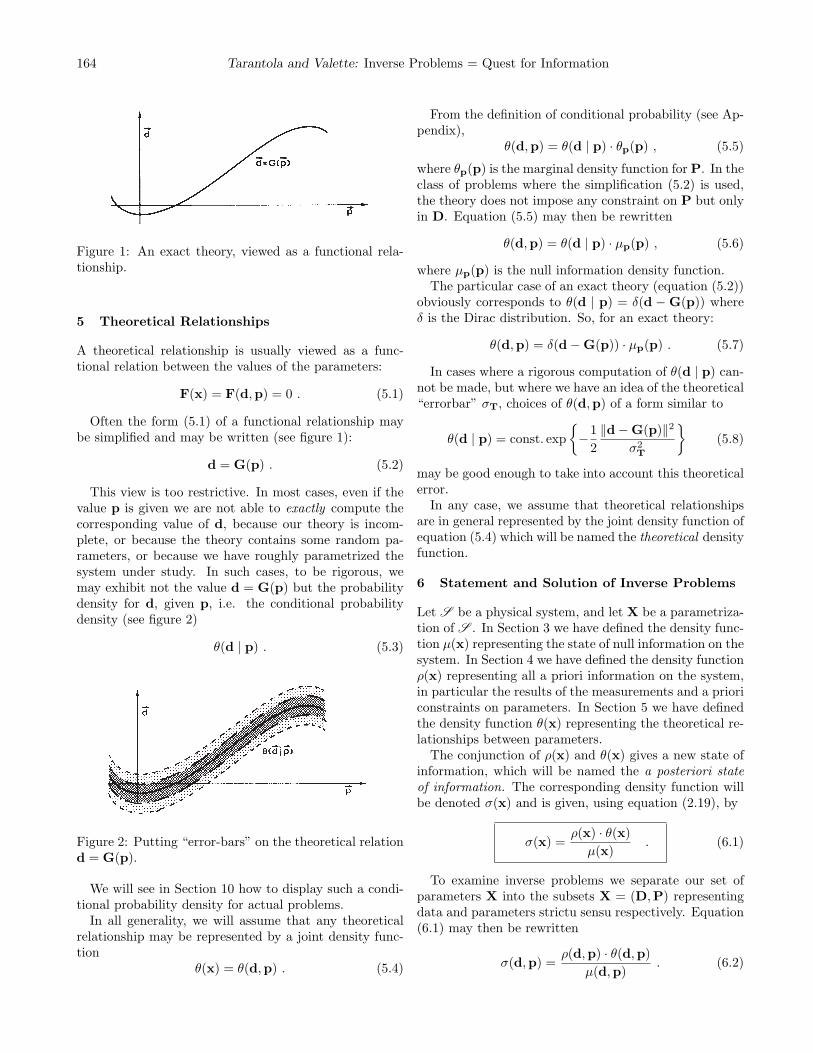
Figure 1: An exact theory, viewed as a functional rela-tionship.

5 Theoretical Relationships

A theoretical relationship is usually viewed as a func-tional relation between the values of the parameters:

F(x) = F(d,p) = 0 . (5.1)

Often the form (5.1) of a functional relationship maybe simplified and may be written (see figure 1):

d = G(p) . (5.2)

This view is too restrictive. In most cases, even if thevalue p is given we are not able to exactly compute thecorresponding value of d, because our theory is incom-plete, or because the theory contains some random pa-rameters, or because we have roughly parametrized thesystem under study. In such cases, to be rigorous, wemay exhibit not the value d = G(p) but the probabilitydensity for d, given p, i.e. the conditional probabilitydensity (see figure 2)

θ(d | p) . (5.3)

Figure 2: Putting “error-bars” on the theoretical relationd = G(p).

We will see in Section 10 how to display such a condi-tional probability density for actual problems.

In all generality, we will assume that any theoreticalrelationship may be represented by a joint density func-tion

θ(x) = θ(d,p) . (5.4)

From the definition of conditional probability (see Ap-pendix),

θ(d,p) = θ(d | p) · θp(p) , (5.5)

where θp(p) is the marginal density function for P. In theclass of problems where the simplification (5.2) is used,the theory does not impose any constraint on P but onlyin D. Equation (5.5) may then be rewritten

θ(d,p) = θ(d | p) · µp(p) , (5.6)

where µp(p) is the null information density function.The particular case of an exact theory (equation (5.2))

obviously corresponds to θ(d | p) = δ(d −G(p)) whereδ is the Dirac distribution. So, for an exact theory:

θ(d,p) = δ(d−G(p)) · µp(p) . (5.7)

In cases where a rigorous computation of θ(d | p) can-not be made, but where we have an idea of the theoretical“errorbar” σT, choices of θ(d,p) of a form similar to

θ(d | p) = const. exp{−1

2‖d−G(p)‖2

σ2T

}(5.8)

may be good enough to take into account this theoreticalerror.

In any case, we assume that theoretical relationshipsare in general represented by the joint density function ofequation (5.4) which will be named the theoretical densityfunction.

6 Statement and Solution of Inverse Problems

Let S be a physical system, and let X be a parametriza-tion of S . In Section 3 we have defined the density func-tion µ(x) representing the state of null information on thesystem. In Section 4 we have defined the density functionρ(x) representing all a priori information on the system,in particular the results of the measurements and a prioriconstraints on parameters. In Section 5 we have definedthe density function θ(x) representing the theoretical re-lationships between parameters.

The conjunction of ρ(x) and θ(x) gives a new state ofinformation, which will be named the a posteriori stateof information. The corresponding density function willbe denoted σ(x) and is given, using equation (2.19), by

σ(x) =ρ(x) · θ(x)µ(x)

. (6.1)

To examine inverse problems we separate our set ofparameters X into the subsets X = (D,P) representingdata and parameters strictu sensu respectively. Equation(6.1) may then be rewritten

σ(d,p) =ρ(d,p) · θ(d,p)

µ(d,p). (6.2)

Journal of Geophysics, 1982, 50, p. 159–170 165

From this equation we may compute the a posteriorimarginal density functions:

σd(d) =∫ρ(d,p) · θ(d,p)

µ(d,p)dp , (6.3)

σp(p) =∫ρ(d,p) · θ(d,p)

µ(d,p)dd . (6.4)

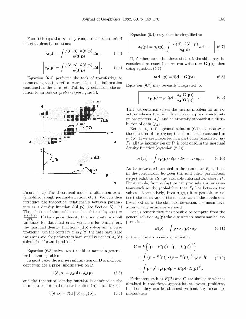
Equation (6.4) performs the task of transferring toparameters, via theoretical correlations, the informationcontained in the data set. This is, by definition, the so-lution to an inverse problem (see figure 3).

Figure 3: a) The theoretical model is often non exact(simplified, rough parameterization, etc.). We can thenintroduce the theoretical relationship between parame-ters as a density function θ(d,p) (see Section 5). b)The solution of the problem is then defined by σ(x) =ρ(x)·θ(x)µ(x) . If the a priori density function contains small

variances for data and great variances for parameters,the marginal density function σp(p) solves an “inverseproblem”. On the contrary, if in ρ(x) the data have largevariances and the parameters have small variances, σd(d)solves the “forward problem.”

Equation (6.3) solves what could be named a general-ized forward problem.

In most cases the a priori information on D is indepen-dent from the a priori information on P,

ρ(d,p) = ρd(d) · ρp(p) (6.5)

and the theoretical density function is obtained in theform of a conditional density function (equation (5.6)):

θ(d,p) = θ(d | p) · µp(p) . (6.6)

Equation (6.4) may then be simplified to

σp(p) = ρp(p) ·∫ρd(d) · θ(d | p)

µd(d)dd . (6.7)

If, furthermore, the theoretical relationship may beconsidered as exact (i.e. we can write d = G(p)), thenusing equation (5.7).

θ(d | p) = δ(d−G(p)) . (6.8)

Equation (6.7) may be easily integrated to:

σp(p) = ρp(p) · ρd(G(p))µd(G(p))

. (6.9)

This last equation solves the inverse problem for an ex-act, non-linear theory with arbitrary a priori constraintson parameters (ρp), and an arbitrary probabilistic distri-bution of data (ρd).

Returning to the general solution (6.4) let us answerthe question of displaying the information contained inσp(p). If we are interested in a particular parameter, sayP1, all the information on P1 is contained in the marginaldensity function (equation (2.5)):

σ1(p1) =∫σp(p) · dp2 · dp3 · . . . · dps . (6.10)

As far as we are interested in the parameter P1 and notin the correlations between this and other parameters,σ1(p1) exhibits all the available information about P1.For example, from σ1(p1) we can precisely answer ques-tions such as the probability that P1 lies between twovalues. Alternatively, from σ1(p1) it is possible to ex-tract the mean value, the median value, the maximum-likelihood value, the standard deviation, the mean devi-ation, or any estimator we need.

Let us remark that it is possible to compute from thegeneral solution σp(p) the a posteriori mathematical ex-pectation:

E(p) =∫

p · σp(p) · dp (6.11)

or the a posteriori covariance matrix:

C = E{(

p− E(p))·(p− E(p)

)T}=∫ (

p− E(p))·(p− E(p)

)Tσp(p)dp

=∫

p · pTσp(p)dp− E(p) · E(p)T .

(6.12)

Estimators such as E(P) and C are similar to what isobtained in traditional approaches to inverse problems,but here they can be obtained without any linear ap-proximation.

166 Tarantola and Valette: Inverse Problems = Quest for Information

7 Existence, Uniqueness, Consistency, Robust-ness, Resolution

In inverse problem theory, it is not always possible toprove the existence or the uniqueness of the solution.With our approach, the existence of the solution is merelythe existence of the a posteriori density function σ(x) ofequation (6.1) and results trivially from the assumptionof the existence of ρ(x) and θ(x). Of course we can obtaina solution σ(x) with some pathologies (non-normalizable,infinite variance, not unique maximum likelihood point,etc.), but the solution is the a posteriori density function,with all the pathologies it may present.

Consistency is warranted because equation (6.1) is con-sistent, i.e. the function σ(x) is a density function. Letus suppose again that we use velocity as a parameter andobtain as solution the density function σ(v), then usingthe same data in the same problem (with the same dis-cretization) but using slowness as parameter we obtainas a solution the density function σ′(n). Since equation(6.1) is consistent, σ′(n) will be related to σ(v) by theusual formula (2.3) σ′(n) = σ(v) · | dvdn |: σ

′(n) and σ(v)represent exactly the same state of information.

In those approaches where all the information con-tained in the data is condensed into the form of centralestimators (mean, median, etc.), the notion of robust-ness must be carefully examined if we suspect that theremay be blunders in the data set (Clearbout and Muir,1973). In our approach, the suspicion of the presenceof blunders in a data set may be introduced using long-tailed density functions in ρd(d), decreasing much moreslowly than gaussian functions as, for example, exponen-tial functions. Our experience shows that with such long-tailed functions, the solution σp(p) is rather insensitiveto one blunder.

The concept of resolution must be considered undertwo different aspects: to what extent a given parameterhas been “resolved” by the data? and what is the “spatialresolution” attained with our data set?

For the first aspect, let us consider a parameter Piwhose value does not influence the values of the data.This means that the theoretical density function θ(d,p)does not depend on Pi. Even in this case we can ob-tain a certain amount of information on this parameter,if the other parameters are resolved by the data, and ifthe a priori density function ρp(p) introduces some corre-lation between parameters. Furthermore, let us assumethat no correlation is introduced by ρp(p) between Piand the other parameters. This is the worst case of non-resolution we can imagine for a parameter. Under theseassumptions equation (6.7) can be written

σp(p) = ρi(Pi) · ρq(q) ·∫ρ(d) · θ(d | q)

µd(d)dd , (7.1)

where q is the vector (p1, . . . , pi−1, pi+1, . . . , ps). After

integration over the set of q, we find (dropping the mul-tiplicative constant):

σi(pi)

= ρi(pi), (7.2)

which means that for a completely unresolved parameter,the a posteriori marginal density function equals the apriori one. The more σi(pi) differs from ρi(pi), the morethe parameter Pi has been resolved by the data set.

The concept of spatial resolution applies to a differentproblem: Assume that Pi, . . . , Pj form a set of parametersspatially (or temporally) distributed as for example whenthe parameters represent the seismic velocities of succes-sive geologic layers (or values from the sampling of somecontinuous geophysical record). Assume that we are notinterested in obtaining the a posteriori density functionfor each parameter, but only the a posteriori mean val-ues, as given by equation (6.11). There are two reasonsfor E(P) to be a smooth vector (i.e. to have small vari-ations between consecutive values E(Pi) and E(Pi+1).The first reason may be the type of data used; it is wellknown for instance that long period surface wave dataonly give a smoothed vision of the Earth. The secondreason for obtaining a smoothed solution may simply bethat we decide a priori to impose such smoothness intro-ducing non null a priori covariances in ρp(p) (see section4).

This question of spatial resolution has been clearlypointed out, and extensively studied by Backus andGilbert (1970). From our point of view, this problemmust be solved by studying the a posteriori correlationsbetween parameters. From equation (6.12):

Cij =∫pi ·pj ·σ

(pi, pj

)·d pi ·d pj−E

(pi)·E(pj). (7.3)

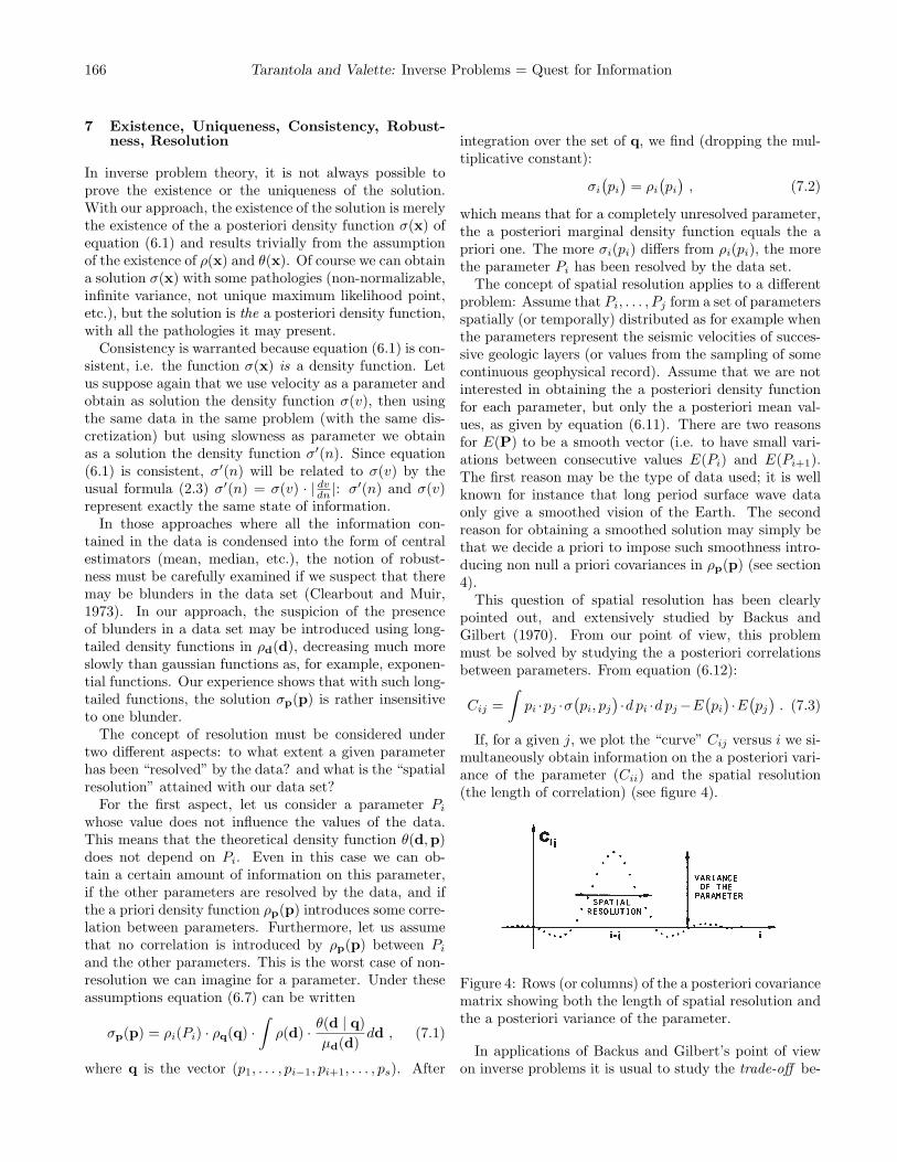
If, for a given j, we plot the “curve” Cij versus i we si-multaneously obtain information on the a posteriori vari-ance of the parameter (Cii) and the spatial resolution(the length of correlation) (see figure 4).

Figure 4: Rows (or columns) of the a posteriori covariancematrix showing both the length of spatial resolution andthe a posteriori variance of the parameter.

In applications of Backus and Gilbert’s point of viewon inverse problems it is usual to study the trade-off be-

Journal of Geophysics, 1982, 50, p. 159–170 167

tween variance and resolution in order to choose the de-sired solution. In our approach, such a trade-off alsoexists: modifying the a priori variances or a priori corre-lations of parameters (in ρ(p)) results in a change of the aposteriori variances and resolutions. But, in our opinion,the a priori information on the values of parameters, ascontained in ρ(p), must not be stated in order to obtaina pleasant solution, but in order to closely correspond tothe actual a priori information.

8 Computational Aspects

For linear problems, all the integrations of section 6 canoften be performed analytically, and the most generalsolution can sometimes be reached easily (see for examplethe next section). Linear procedures may of course beused to obtain adequate approximations for the solutionof weakly nonlinear problems.

For non-linear problems, the solution is less straight-forward. Often the integrations in equation (6.4) or (6.7)can be performed analytically, no matter what the degreeof nonlinearity (see for example section 10). The compu-tation of the density of probability σp(p) at a given pointp then involves mainly the solution of a forward prob-lem. If the number of parameters is small we can thenexplicitly compute the marginal probability density foreach one of the parameters, using agrid in the parameterspace ordinary methods of numerical integration. If thenumber of parameters is great, Monte-Carlo methods ofnumerical integration should be used. The possibility ofconveniently solving non-linear inverse problems will thendepend on the possibility of solving the forward problema large enough number of times. Let us remark that if weare not able to compute the marginal probability densityfor each one of the parameters of interest, we can limitourselves to the computation of mean values and covari-ances (equations (6.11) and (6.12).

In problems where the solution of the forward prob-lem is so costly that either the explicit computation ofthe density of probability in the parameter space andthe computation of mean values and covariances cannotbe performed in a reasonable computer time, we suggestto restrict the problem to the search of the maximumlikelihood point in the parameter space (point at whichthe density of probability is maximum). This computa-tion is often very easy to perform, and classical meth-ods can be used for particular assumptions about theform of the probability densities representing experimen-tal data and a priori assumptions on parameters. Forexample, it is easy to see that with gaussian assump-tions, the search of the maximum likelihood point simplybecomes a classical leastsquares problem (Tarantola andValette, 1982). With exponential assumptions, the searchof the maxima likelihood point becomes a L1-norm prob-

lem (which shows that the exponential assumption givesa result more robust than the gaussian one). With theuse of step functions, the a posteriori probability densityin the parameter space is constant inside a given boundeddomain. The point of this domain the maximizes somefunction of the parameters can be reached using the lin-ear (or non-linear) programming techniques. We see thusthat ordinary methods for solving parameterized inverseproblems can be deduced as particular cases of our ap-proach, and we want to emphasize that such methodsshould only be used when the explicit computation ofthe density of probability in the parameter space or thenon-linear computation of mean values and covarianceswould be too much time consuming.

9 Gaussian Case

Since the gaussian linear problem is widely used, we willshow how the usual formulae may be derived from ourresults.

By gaussian problem we mean that the a priori densityfunction has a gaussian form for all parameters:

ρ(x) = exp{−1

2(x− x0

)T ·C−10 ·

(x− x0

)}, (9.1)

where x0 is the a priori expected value and C0, is the apriori covariance matrix.

By the linear problem we mean that if the theory maybe assumed to be exact, the theoretical relationship be-tween parameters takes the general linear form:

F · x = 0 . (9.2)

On the other hand, if theroretical errors may not be ne-glected, we assume that the theoretical density functionalso has a gaussian form:

θ(x) = exp{−1

2(F · x)T ·C−1

T · (F · x)}, (9.3)

where the covariance matrix CT describes theoretical er-rors (and tends to vanish for an exact theory).

We finally assume that for the parameters chosen, thenull information is represented by a constant function:

µ(x) = const. (9.4)

The a posteriori density function (equation (6.1) is thengiven by:

σ(x) = ρ(x) · θ(x)

= exp{− 1

2

[(x− x0

)T ·C−10 ·

(x− x0

)+ xT · FT ·C−1

T · F · x]} (9.5)

168 Tarantola and Valette: Inverse Problems = Quest for Information

and after some matrix manipulations, (see appendix) weobtain

σ(x) = exp{−1

2(x− x∗

)T ·C−1∗ ·

(x− x∗

)}, (9.6)

where

x∗ = P · x0, (9.7)

C∗ = P ·C0 (9.8)

and

P = I−Q

Q = C0 · FT ·(F ·C0 · FT + CT

)−1 · F .(9.9)

Equation (9.6) shows that the a posteriori density func-tion is gaussian, centered in x∗ and with the covariancematrix C∗.

If theoretical errors may be neglected, i.e. if equation(9.2) holds, we just drop the term CT in equation (9.9)to obtain the corresponding solution.

To compare our results to those published in the lit-erature, let us assume that the separation of X into thesets D and P is made:

x =[dp

]x0 =

[d0

p0

]x∗ =

[d∗

p∗

]C0 =

[Cdd Cdp

Cpd Cpp

].

(9.10)

We also assume that equation (9.2) simplifies to:

F · x = [I−G] ·[dp

]= d−G · p = 0 . (9.11)

Substituting equations (9.10), (9.11) in equations (9.7),(9.8), (9.9) we obtain the solution published by Franklin(1970) for the parametrized problem, which was obtainedusing the classical least squares approach. Our equations(9.7), (9.8), (9.9) are more compact than those of Franklinbecause we use the parameter space Em, and more gen-eral because we allow theoretical errors CT.

Let us emphasize that in traditional approaches x∗, isinterpreted as the best estimator of the “true” solutionand C∗ is interpreted as the covariance matrix of the esti-mator. Our approach demonstrates that the a posterioridensity function is gaussian, and that x∗ and C∗ are, re-spectively, the center and the disnersion of the densityfunction.

The results shown here only apply to the linear leastsquares problem. For the non-linear problem, the readershould refer to Tarantola and Valette (1982).

station x y z t σt1 49.58 9.54 −0.80 13.35 0.022 48.07 7.74 −0.80 13.30 0.023 49.67 4.22 −1.50 13.79 0.024 52.34 14.37 −0.30 13.70 0.025 43.17 5.70 −0.80 13.90 0.026 46.79 17.87 −0.30 14.35 0.027 48.82 −1.87 −0.90 14.20 0.108 33.31 8.72 −0.60 15.41 0.029 23.10 9.54 −0.50 17.09 0.0210 13.24 15.30 −0.40 19.00 0.1011 −2.19 11.41 −1.20 18.73 0.02

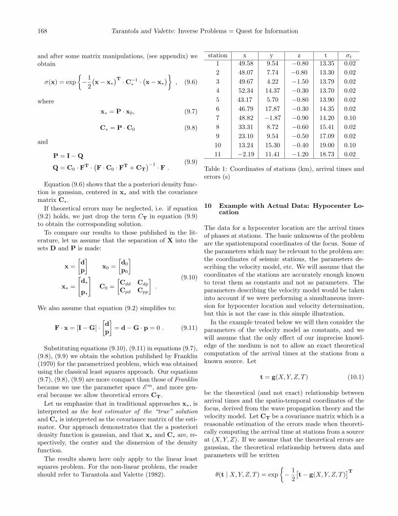
Table 1: Coordinates of stations (km), arrival times anderrors (s)

10 Example with Actual Data: Hypocenter Lo-cation

The data for a hypocenter location are the arrival timesof phases at stations. The basic unknowns of the problemare the spatiotemporal coordinates of the focus. Some ofthe parameters which may be relevant to the problem are:the coordinates of seismic stations, the parameters de-scribing the velocity model, etc. We will assume that thecoordinates of the stations are accurately enough knownto treat them as constants and not as parameters. Theparameters describing the velocity model would be takeninto account if we were performing a simultaneous inver-sion for hypocenter location and velocity determination,but this is not the case in this simple illustration.

In the example treated below we will then consider theparameters of the velocity model as constants, and wewill assume that the only effect of our imprecise knowl-edge of the medium is not to allow an exact theoreticalcomputation of the arrival times at the stations from aknown source. Let

t = g(X,Y, Z, T ) (10.1)

be the theoretical (and not exact) relationship betweenarrival times and the spatio-temporal coordinates of thefocus, derived from the wave propagation theory and thevelocity model. Let CT be a covariance matrix which is areasonable estimation of the errors made when theoreti-cally computing the arrival time at stations from a sourceat (X,Y, Z). If we assume that the theoretical errors aregaussian, the theoretical relationship between data andparameters will be written

θ(t | X,Y, Z, T ) = exp{− 1

2[t− g(X,Y, Z, T )

]T

Journal of Geophysics, 1982, 50, p. 159–170 169

·C−1T ·

[t− g(X,Y, Z, T )

]}, (10.2)

which correspond to equation (5.8).The next simplifying hypothesis is to assume that our

data possess a gaussian structure. Let t0 be their vectorof mean values and Ct, their covariance matrix:

ρ(t) = exp{− 1

2(t− t0

)T ·C−1t ·

(t− t0

)}. (10.3)

As all our data and parameters consist in Cartesianspacetime coordinates, the null information function isconstant and need not be considered (see section 3).

The a posteriori density function for parameters is di-rectly given by equation (6.7) and after analytical inte-gration we obtain (see appendix):

σ(X,Y, Z, T ) = ρ(X,Y, Z, T )·

· exp{− 1

2(t0 − g(X,Y, Z, T )

)T · (Ct + CT

)−1·

·(t0 − g(X,Y, Z, T )

)}. (10.4)

The a posteriori density function (10.4) gives the gen-eral solution for the problem of spatio-temporal hypocen-ter location in the case of gaussian data. We emphasizethat this solution does not contain any “linear approxi-mation”.

We are sometimes interested in the spatial location ofthe quake focus, and not in its temporal location. Thedensity function for the spatial coordinates is obtained,of course, by the marginal density function

σ(X,Y, Z) =∫ +∞

−∞σ(X,Y, Z, T )dT , (10.5)

where we integrate over the range of the origin time T .Classical least squares computations of hypocenter are

based on the maximization of σ(X,Y, Z, T ). It is clearthat if we are only interested in the spatial location wemust maximize σ(X,Y, Z) given by (10.5) instead of max-imizing σ(X,Y, Z, T ). Let us show how the integrationin (10.5) can be performed analytically.

We will assume that while we may sometimes have apriori information about the spatial location of the focus(from tectonic arguments, or from past experience in theregion, etc.) it is generally impossible to have a prioriinformation (independent from the data) about the origintime T . We will thus assume an a priori density functionuniform on T ,

ρ(X,Y, Z, T ) = ρ(T ) · ρ(X,Y, Z) = ρ(X,Y, Z) . (10.6)

The computed arrival time at a station i, gi(X,Y, Z, T )can be written

gi(X,Y, Z, T ) = hi(X,Y, Z) + T , (10.7)

where hi is the travel time between the point (X,Y, Z)and the station i.

With (10.6) and (10.7), equation (10.5) can be inte-grated (see appendix) and gives

σ(X,Y, Z) = K · ρ(X,Y, Z)

· exp{− 1

2[t0 − h(X,Y, Z)

]T·P ·

[t0 − h(X,Y, Z)

]}.

(10.8)

HereP = (Ct + CT)−1 (10.9)

is a“weight matrix”,

pi =∑j

Pij (10.10)

are “weights”, and

K =∑i

pi =∑ij

Pij . (10.11)

Moreover, ti0 is the observed arrival time minus theweighted mean of observed arrival times,

ti0 = ti0 −∑j pjt

j0∑

j pj(10.12)

and hi(X,Y, Z) is the computed travel time minus theweighted mean of computed travel times

hi = hi −∑j pjh

j∑j pj

. (10.13)

(Note that CT may depend on (X,Y, Z) and thereforePij , pi, and K also.)

Equation (10.8) gives the general solution for the spa-tial location of a quake focus in the Gaussian case.

Table 1 shows the observed arrival times and their stan-dard deviation. We have assumed that the theoreticalerrors are of the form :

[CT(X,Y, Z)

]ij

= σ2T · exp

{−1

2D2ij

∆2

}, (10.14)

where Dij is the distance between the station i and thestation j, σT is some theoretical error, and ∆ is the cor-relation length of errors (the wavelength or the length oflateral heterogeneities of the medium). By comparisonof the layered model of velocities for the Western Pyre-nees (Gagnepain et al., 1980) with data from refractionprofiles (Gallart, 1980) we have chosen σT = 0.2 s and∆ = 0.1 km.

170 Tarantola and Valette: Inverse Problems = Quest for Information

We also assumed that no a priori information is knownabout the epicenter, but that we know that the depthof the hypocenter is greater than −0.5 km (the meantopography):

ρ(X,Y, Z) = ρ(Z) =

{1 if Z = −0.5 km

0 if Z < −0.5 km .(10.15)

We have then computed numerically from (10.8) thea posteriori marginal density functions for the epicenterand for the depth:

σ(X,Y ) =∫ +∞

−0.5km

σ(X,Y, Z)dZ, (10.16)

σ(Z) =∫ +∞

−∞dX

∫ +∞

−∞dY σ(X,Y, Z) . (10.17)

The results are shown in figures 5 and 6.

Figure 5: a. and b. Results of the inverse problemof hypocenter computation. a. shows the position ofthe stations and the probability density obtained for theepicentral coordinates. b. shows the computer output.Curves are visual interpolations.

We have also computed mean values and variances.The corresponding results are, in the local frame of fig-ure 5:

E(X) = 51.7 km σX = 1.5 kmE(Y ) = 7.8 km σY = 0.9 kmE(Z) = 5.6 km σZ = 2.1 km .

Figure 6: The probability density for depth. The layeredvelocity model is also shown. Note the existence of asecondary maximum likelihood point.

We wish to make the following remarks about these re-sults.

First, they have been obtained exactly without the useof linear approximations. We have used numerical inte-gration instead of matrix algebra and the computation ofpartial derivatives. The results shown in figures 5 and 6represent the most general knowledge which can be ob-tained for the hypocenter coordinates from the arrivaltimes, from the given velocity model, and from the giventheoretical model (of wave propagation).

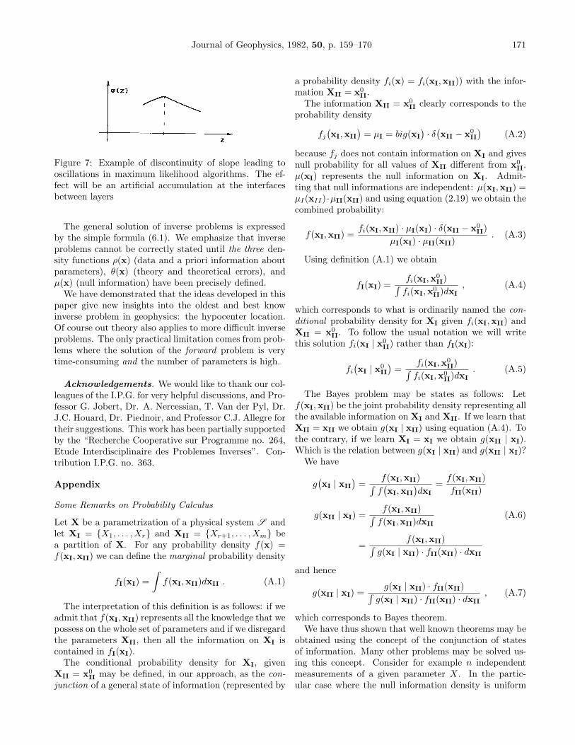
Since the velocity model is discontinuous in Z the aposteriori density functions have discontinuities in slope,as it is clearly seen in figure 6 for σ(Z) To the extent thatthe discontinuities in the velocity model are artificial, thediscontinuities of slope are of course also artificial. Fromfigure 6 it is easy to visualize some of the problems whichmay affect the maximum likelihood approach. If the dis-continuity of slope is similar to the one at 5 km depth,we will have secondary maxima. We can also have a dis-continuity of slope of the type drawn in figure 7. In thatcase, algorithms searching for the maximum likelihoodpoint will oscillate arount the point of slope discontinu-ity, leading to the well-known artificial situation in whichhypocenters accumulate at the interface between layersof constant velocity.

11 Conclusion

Our informational approach to probability calculus allowsus to formulate inverse problems in such a way that allnecessary constraints (see Section 1) are satisfied. Essen-tially, we propose to work with the probability densitiesfor parameters rather than with central estimators, as itis usually done.

Journal of Geophysics, 1982, 50, p. 159–170 171

Figure 7: Example of discontinuity of slope leading tooscillations in maximum likelihood algorithms. The ef-fect will be an artificial accumulation at the interfacesbetween layers

The general solution of inverse problems is expressedby the simple formula (6.1). We emphasize that inverseproblems cannot be correctly stated until the three den-sity functions ρ(x) (data and a priori information aboutparameters), θ(x) (theory and theoretical errors), andµ(x) (null information) have been precisely defined.

We have demonstrated that the ideas developed in thispaper give new insights into the oldest and best knowinverse problem in geophysics: the hypocenter location.Of course out theory also applies to more difficult inverseproblems. The only practical limitation comes from prob-lems where the solution of the forward problem is verytime-consuming and the number of parameters is high.

Acknowledgements. We would like to thank our col-leagues of the I.P.G. for very helpful discussions, and Pro-fessor G. Jobert, Dr. A. Nercessian, T. Van der Pyl, Dr.J.C. Houard, Dr. Piednoir, and Professor C.J. Allegre fortheir suggestions. This work has been partially supportedby the “Recherche Cooperative sur Programme no. 264,Etude Interdisciplinaire des Problemes Inverses”. Con-tribution I.P.G. no. 363.

Appendix

Some Remarks on Probability Calculus

Let X be a parametrization of a physical system S andlet XI = {X1, . . . , Xr} and XII = {Xr+1, . . . , Xm} bea partition of X. For any probability density f(x) =f(xI,xII) we can define the marginal probability density

fI(xI) =∫f(xI,xII)dxII . (A.1)

The interpretation of this definition is as follows: if weadmit that f(xI,xII) represents all the knowledge that wepossess on the whole set of parameters and if we disregardthe parameters XII, then all the information on XI iscontained in fI(xI).

The conditional probability density for XI, givenXII = x0

II may be defined, in our approach, as the con-junction of a general state of information (represented by

a probability density fi(x) = fi(xI,xII)) with the infor-mation XII = x0

II.The information XII = x0

II clearly corresponds to theprobability density

fj(xI,xII

)= µI = big(xI

)· δ(xII − x0

II

)(A.2)

because fj does not contain information on XI and givesnull probability for all values of XII different from x0

II.µ(xI) represents the null information on XI. Admit-ting that null informations are independent: µ(xI,xII) =µI(xII) ·µII(xII) and using equation (2.19) we obtain thecombined probability:

f(xI,xII) =fi(xI,xII) · µI(xI) · δ(xII − x0

II)µI(xI) · µII(xII)

. (A.3)

Using definition (A.1) we obtain

fI(xI) =fi(xI,x0

II)∫fi(xI,x0

II)dxI, (A.4)

which corresponds to what is ordinarily named the con-ditional probability density for XI given fi(xI,xII) andXII = x0

II. To follow the usual notation we will writethis solution fi(xI | x0

II) rather than fI(xI):

fi(xI | x0

II

)=

fi(xI,x0II)∫

fi(xI,x0II)dxI

. (A.5)

The Bayes problem may be states as follows: Letf(xI,xII) be the joint probability density representing allthe available information on XI and XII. If we learn thatXII = xII we obtain g(xI | xII) using equation (A.4). Tothe contrary, if we learn XI = xI we obtain g(xII | xI).Which is the relation between g(xI | xII) and g(xII | xI)?

We have

g(xI | xII

)=

f(xI,xII)∫f(xI,xII

)dxI

=f(xI,xII)fII(xII)

g(xII | xI) =f(xI,xII)∫f(xI,xII)dxII

=f(xI,xII)∫

g(xI | xII) · fII(xII) · dxII

(A.6)

and hence

g(xII | xI) =g(xI | xII) · fII(xII)∫

g(xI | xII) · fII(xII) · dxII, (A.7)

which corresponds to Bayes theorem.We have thus shown that well known theorems may be

obtained using the concept of the conjunction of statesof information. Many other problems may be solved us-ing this concept. Consider for example n independentmeasurements of a given parameter X. In the partic-ular case where the null information density is uniform

172 Tarantola and Valette: Inverse Problems = Quest for Information

(µ(x) = const.), and each measurement gives a gaussianprobability density fi(x) centered at xi and with varianceσ2

fi(x) =1√2πσ

exp{−1

2(x− xi)2

σ2

}, (A.8)

the iteration of equation (2.19) at each new measurementgives

f(x) =1√2πΣ

exp{−1

2(x− x)2

Σ2

}, (A.9)

where

x =Σxin

Σ =σ√n, (A.10)

which are well known results in statistics.

Demonstrations for Section 9

Let us first demonstrate two useful identities. If C1 andC2 are two positive definite matrices respectively of order(n×n) and (m×m), and M an arbitrary (n×m) matrix,then: (

MTC−11 M + C−1

2

)−1MTC−1

1

= C2MT(C1 + MC2MT

)−1,

(A.11)

(MTC−1

1 M + C−12

)−1 = C2 −C2MT

×(C1 + MC2MT

)−1MC2.

(A.12)

The first equation follows from the following obviousidentities

MT + MTC−11 MC2MT

= MTC−11

(C1 + MC2MT

)=(MTC−1

1 M + C−12

)C2MT

(A.13)

since MTC−11 M + C−1

2 and C1 + MC2MT are definitepositive and thus regular matrices.

Furthermore (A.11) leads to

C2 −C2MT(C1 + MC2MT

)−1MC2

= C2 −(MTC−1

1 M + C−12

)−1MTC−1

1 MC2

=(MTC−1

1 M + C−12 )−1

×{(

MTC−11 M + C−1

2

)C2 −MTC−1

1 MC2

}=(MTC−1

1 M + C−12

)−1

(A.14)

which proves (A.12).

Now from equation (9.5) we obtain:

σ(x) = exp{− 1

2

[(x− x0

)TC−1

0

(x− x0

)+ xTFTC−1

T Fx]}

= exp{− 1

2

[xT(C−1

0 + FTC−1T F

)x

− 2xTC−10 x0 + xT

0 C−10 x0

]}(A.15)

then defining:

P = I−C0FT(FC0FT + CT

)−1F, (A.16)

C∗ = PC0, (A.17)

x∗ = Px0. (A.18)

We obtain, using equation (A.12)

C∗ = PC0

= C0 −C0FT(FC0FT + CT

)−1FC0

=(FTC−1

T F + C−10

)−1

(A.19)

andx∗ = Px0 = C∗C−1

0 x0. (A.20)

Thus equation (A.15) becomes:

σ(x) = exp{− 1

2(xTC−1

∗ x− 2xTC−1∗ x∗

+ xT0 C−1∗ x∗

)}= exp

{− 1

2

[(x− x∗

)TC−1∗(x− x∗

)−(x∗ − x0

)TC−1

0 x0

]}.

(A.21)

From (A.18), we deduce:

x∗ − x0 = −C0FT(FC0FT + CT

)−1FC0x0 (A.22)

and then:

σ(x) = exp{− 1

2xT

0 FT(FC0FT + CT

)−1Fx0

}· exp

{− 1

2(x− x∗

)TC−1∗(x− x∗

)}= const. exp

{− 1

2(x− x∗

)TC−1∗(x− x∗

)}(A.23)

which demonstrates equation (9.6).

Journal of Geophysics, 1982, 50, p. 159–170 173

Demonstrations for Section 10

Let us now evaluate the sum:

I =∫

exp

×{− 1

2

[(d− d0

)TC−1

d

(d− d0

)+(d− g(p)

)TC−1

T

(d− g(p)

)]}dd.

(A.24)

The separation of the quadratic terms from the linearterms leads to:

I =∫

exp{− 1

2(dTAd− 2BTd + C

)}dd (A.25)

where:

A = C−1d + C−1

T

BT = dT0 C−1

d + g(p)TC−1T

C = dT0 C−1

d d0 + g(p)TC−1T g(p).

(A.26)

Since A is positive definite there follows:

I =∫

exp{− 1

2

[(d−A−1B

)TA(d−A−1B

)+(C−BTA−1B

)]}dd

= exp{− 1

2(C−BTA−1B

)}×∫

exp{− 1

2(d−A−1B

)TA(d−A−1B

)}dd

= (2π)n/2(det A)−1/2 exp{− 1

2(C−BTA−1B

)}.

(A.27)

By substitution of (A.26) we obtain:

C−BTA−1B

= dT0

(C−1

d −C−1d

(C−1

d + C−1T

)C−1

d

)d0

+ g(p)T(C−1

T −C−1T

(C−1

d + C−1T

)C−1

T

)g(p)

− 2g(p)C−1T

(C−1

d + C−1T

)C−1

d d0.

(A.28)

Thus, by using the two identities ((A.11)-(A.12)) we get:

C−BTA−1B

= d0

(Cd + CT

)−1d0 + g(p)T

(Cd + CT

)−1g(p)

− 2g(p)(Cd + CT

)−1d0

=(d0 − g(p)

)T(Cd + CT

)−1(d0 − g(p)

).

(A.29)

Finally we obtain:

I = (2π)n/2 ·[

det(C−1

d + C−1T

)]−1/2

· exp{− 1

2(d0 − g(p)

)T(Cd + CT

)−1

×(d0 − g(p)

)} (A.30)

which demonstrates equation (10.4).Let us define

P =(Ct + CT

)−1. (A.31)

Using (10.4) and (10.7), the sum (10.5) becomes:

I =∫

exp{− 1

2

∑ij

[t0i − hi − T

]· Pij ·

[t0j − hj − T

]}dT

=∫

exp{− 1

2(dT 2 − 2b T + c

)}dT

(A.32)

where :

a =∑ij

Pij

b =∑ij

Pij ·(t0j − hj

)c =

∑ij

(t0j − hj

)· Pij ·

(t0j − hj

).

(A.33)

This yields :

I =∫

exp

{−1

2

[a

(T − b

a

)2

+(c− b2

a

)]}dT

=(

2πa

)1/2

exp{−1

2

(c− b2

a

)}.

(A.34)

By substitution of a, b and c given in (A.33) in the aboveexpression, we obtain:

I =(

2πΣijPij

)1/2

· exp

{− 1

2

[∑ij

(t0j − hj

)· Pij ·

(t0i − hi

)−

[∑ij Pij · (t0j − hj)]2

ΣijPij

]}(A.35)

174 Tarantola and Valette: Inverse Problems = Quest for Information

which can also be written:

I =

(2π∑ij Pij

)1/2

· exp

{− 1

2

∑ij

[t0i − hi −

∑kl Pkl(t

0l − hl)∑

kl Pkl

]

· Pij ·[t0j − hj −

∑kl Pkl(t

0l − hl)∑

kl Pkl

]}(A.36)

or

I =

(2π∑ij Pij

)1/2

· exp

−12

∑ij

(t0i − hi

)· Pij ·

(t0j − hj

)(A.37)

where

t0i = t0i −∑kl Pkl · t0l∑kl Pkl

hi = hi −∑kl Pkl · hl∑kl Pkl

(A.38)

which is the expression (10.8).

References

Backus, G., Gilbert, F.: Numerical applications of a for-malism for geophysical inverse problems. Geophys.J. R. Astron. soc. 13, 247–276, 1967

Backus, G., Gilbert, F.: The resolving power of grossearth data - Geophys. J. R. Astron. soc. 16, 169–205, 1968

Backus, G., Gilbert, F.: Uniqueness in the inversion ofinaccurate gross earth data. Philos. Trans. R. soc.London 266, 123–192, 1970

Backus, G.: Inference from inadequate and inaccuratedata, Mathematical problems in the Geophysical Sci-ences: Lecture in applied Mathematics, 14, Amer-ican Mathematical Society, Providence, Rhode Is-land, 1971

Clearbout, J.F., Muir, F.: Robust modelling with erraticdata. Geophysics 38, 5, 826–844, 1973

Descombes, R.: Integration. Corollary 6.2, p. 106. Paris:Hermann 1972

Franklin, J.N.: Well posed stochastic extension of illposed linear problems. J. Math. Anal. Applic. 31,682–716, 1970

Gagnepain, J., Modiano, T., Cisternas, A., Ruegg, J.C.,Vadell, M., Hatzfeld, D., Mezcua, J.: Sismicite dela region d’Arette (Pyrenees-Atlantiques) et mecan-ismes au foyer. Ann. Geophys. 36, 499–508, 1980

Gallart, J.: Structure crustale des Pyrenees d’apres lesetudes de sismologie experimentale. Thesis of 3rdcycle. 132 p. Universite Paris VI, 1980

Jackson, D.D.: Interpretation of inaccurate, insufficientand inconsistent data. Geophys. J. R. Astron. soc.28, 97–110, 1972

Jaynes, E.T. : Prior probabilities. I.E.E.E. Transactionson systems, Science and cybernetics. Vol. SSC-4,No. 3, 227–241, 1968

Jeffreys, H.: Theory of probability, Oxford: ClarendonPress 1939

Jeffreys, H. : Scientific Inference, London: CambridgeUniversity Press 1957

Keilis-Borok, V.I., Yanovskaya: Inverse problems in seis-mology, Geophys. J. R. Astron. soc. 13, 223–234,1967

Parker, R.L.: The theory of ideal bodies for gravity inter-pretation. Geophys. J. R. Astron. soc. 42, 315–334,1975

Rietsch, E.: The maximum entropy approach to InverseProblems. J. Geophys. 42, 489–506, 1977

Sabatier, P.C.: On geophysical inverse problems and con-straints. J. Geophys. 43, 115–137, 1977

Shannon, C.E.: A mathematical theory of communica-tion - Bell System Tech. J. 27, 379–423, 1948

Tarantola, A., Valette, B.: Generalized non linear in-verse problems solved using the least squares crite-rion. Rev. Geophys. Space Phys., 19, No. 2, 1982(in press)

Wiggins, R.A.: The general inverse problem: implicationof surface waves and free oscillations for earth struc-ture. Rev. Geophys. Space Phys. 10,251–285, 1972

Received August 21, 1981; Revised version February 1,1982; Accepted February 2, 1982