INVERSIONS OF INTEGRAL OPERATORS AND ELLIPTICBETA INTEGRALS ON ROOT SYSTEMS

VYACHESLAV P. SPIRIDONOV AND S. OLE WARNAAR

Abstract. We prove a novel type of inversion formula for elliptic hypergeo-

metric integrals associated to a pair of root systems. Using the (A,C) inversionformula to invert one of the known C-type elliptic beta integrals, we obtain a

new elliptic beta integral for the root system of type A. Validity of this integral

is established by a different method as well.

Contents

1. Introduction 12. Notation and preliminaries 33. Elliptic beta integrals 44. Inversion formulas. I. The single variable case 64.1. Motivation 64.2. The n = 1 integral inversion 74.3. Proof of Theorem 4.1 95. Inversion formulas. II. The root systems An and Cn 105.1. Main results 105.2. Consequences of Theorems 5.1 and 5.2 135.3. Proof of Theorem 5.2 216. Alternative proof of the new An elliptic beta integral 32References 36

1. Introduction

Beta-type integrals are fundamental objects of applied analysis, with numerousapplications in pure mathematics and mathematical physics. The classical Eulerbeta integral∫ 1

0

tx−1(1− t)y−1dt =Γ(x)Γ(y)Γ(x+ y)

, min{Re(x),Re(y)} > 0,

determines the measure for the Jacobi family of orthogonal polynomials expressedas certain 2F1 hypergeometric functions [3]. Its multi-dimensional extension dueto Selberg [21] plays an important role in harmonic analysis on root systems, the

2000 Mathematics Subject Classification. 33D60, 3367, 33E05.Key words and phrases. Elliptic hypergeometric integrals, beta integrals, elliptic hypergeomet-

ric series.V.P.S. is supported in part by the Russian Foundation for Basic Research (RFBR) grant no.

03-01-00781; S.O.W. is supported by the Australian Research Council.

1

2 VYACHESLAV P. SPIRIDONOV AND S. OLE WARNAAR

theory of special functions of many variables, the theory of random matrices, andso forth.

Important generalizations of beta integrals arise in the theory of basic or q-hypergeometric functions. The Askey–Wilson q-beta integral depends on four in-dependent parameters and a base q, and fixes the orthogonality measure for theAskey–Wilson polynomials, the most general family of classical single-variable or-thogonal polynomials [4]. Closely related to the Askey–Wilson integral is the in-tegral representation for a very-well-poised 8φ7 basic hypergeometric series foundby Nassrallah and Rahman [15]. Through specialization this led Rahman to thediscovery of a one-parameter extension of the Askey–Wilson integral [16]. Finally,several multi-dimensional generalizations of the Askey–Wilson and Rahman inte-grals, including a q-Selberg integral, were found by Gustafson [10, 11, 12]. For sometime, these multi-dimensional q-beta integrals were believed to be the most generalintegrals of beta type.

A new development in the field was initiated by the first author with the discoveryof an elliptic generalization of Rahman’s q-beta integral [22]. This elliptic betaintegral depends on five free parameters and two basic variables — or elliptic moduli— p and q. As a further development two n-dimensional elliptic beta integralsassociated to the Cn root system were proposed by van Diejen and the first author[6, 7]. In the p→ 0 limit these integrals reduce to Gustafson’s Cn q-beta integrals.More elliptic beta integrals, all related to either the An or Cn root systems and allbut one generalizing integrals of Gustafson [11, 12] and Gustafson and Rakha [13],were subsequently given in [26].

Roughly, n-dimensional elliptic beta integrals come in three different types. Mostfundamental are the type-I integrals. These contain 2n + 3 free parameters (aswell as the bases p and q), and one of the An integrals of [24] and one of theCn integrals of [7] are of type I. The first complete proofs were found by Rains[17] who derived them as a consequence of a symmetry transformation for moregeneral elliptic hypergeometric integrals. More elementary proofs using differenceequations were subsequently given in [26]. The elliptic beta integrals of type IIcontain less than 2n + 3 parameters and can be deduced from type I integrals viathe composition of higher-dimensional integrals [7, 10, 12, 13, 24]. The secondCn elliptic beta integral of [7] (see also [6]), depending on six parameters (only 5when n = 1), provides an example of a type II integral. Finally, type III ellipticbeta integrals arise through the computation of n-dimensional determinants withentries composed of one-dimensional integrals [24]. Originally, all of the above betaintegrals were defined for bases p and q inside the unit circle (due to the use of thestandard elliptic gamma function described in the next section). Another class ofelliptic hypergeometric integrals, which are well defined in the larger region |p| < 1,|q| ≤ 1 (by employing a different elliptic gamma function), has been introduced in[24]. We shall not discuss here the corresponding elliptic beta integrals, and referthe reader to [8, 26] for more details.

Further progress on the subject is associated with symmetry transformations ofelliptic hypergeometric integrals. Certain hypergeometric identities are well-knownto be related to the notion of matrix inversions and Bailey pairs. At the level ofhypergeometric series — ordinary, basic or elliptic — the Bailey pair machineryallows for the derivation of infinite sequences of symmetry transformations [1, 2,23, 27, 29]. A formulation of the notion of Bailey pairs for integrals was proposed in

ELLIPTIC BETA INTEGRALS 3

[25] (on the basis of a transformation for univariate elliptic hypergeometric integralsproved in [24]). Using the univariate elliptic beta integral, this led to a binary treeof identities for multiple elliptic hypergeometric integrals. A generalization of theseresults to elliptic hypergeometric integrals labelled by root systems has been one ofthe motivations for the present paper. Indeed, the integral analogues of the matrixinversions underlying the Bailey transform for series are provided by the integralinversions of this paper.

A powerful set of symmetry transformations relating elliptic hypergeometric in-tegrals of various dimensions was introduced by Rains [17]. He proved the latter inan elegant manner by reducing the problem to determinant evaluations on a denseset of parameters. Although some of the Rains transformations can be reproducedwith the help of the Bailey type technique, a complete correspondence betweenthese two sets of identitites has not been established yet.

More specifically, we provide the following new framework for viewing ellipticbeta integrals on root systems. First, we introduce certain multi-dimensional in-tegral transformations with integration kernels determined by the structure of thetype I elliptic beta integrals on the An and Cn root systems. The An and Cnelliptic beta integrals then acquire the new interpretation as examples for whichthese integral transformations can be performed explicitly. Second, we prove twotheorems describing inversions of the corresponding integral operators on a certainclass of functions and conjecture a third inversion formula. These inversion formulasnaturally carry two root system labels, our three results corresponding to the pairs(An,An), (An,Cn) and (Cn,An). Third, using the (An,Cn) inversion formula we‘invert’ the type I Cn beta integral to prove a new type I An elliptic beta integral.It appears that this exact integration formula is new even at the q-hypergeometricand plain hypergeometric levels. Finally, for completeness, we give an alternativeproof of this integral using the method for proving type I integrals developed in[26].

In the univariate case, all three integral inversions coincide and the resultingformula establishes the inversion of the integral Bailey transform of [25]. Also ourmulti-variable integral transformations on root systems can be put into the frame-work of integral Bailey pairs. This will be the topic of a subsequent publicationtogether with a consideration of integral operators associated with the type II el-liptic beta integrals.

2. Notation and preliminaries

Throughout this paper p, q ∈ C such that

(2.1) M := max{|p|, |q|} < 1.

For fixed p and q, and z ∈ C\{0} the elliptic gamma function is defined as [19]

(2.2) Γ(z; p, q) =∞∏

µ,ν=0

1− z−1pµ+1qν+1

1− zpµqν,

and satisfies

Γ(z; p, q) = Γ(z; q, p),(2.3a)

Γ(z; p, q) =1

Γ(pq/z; p, q).(2.3b)

4 VYACHESLAV P. SPIRIDONOV AND S. OLE WARNAAR

Defining the theta function

θ(z; p) = (z, p/z; p)∞,

where

(a; q)∞ =∞∏k=0

(1− aqk) and (a1, . . . , ak; q)n = (a1; q)n · · · (ak; q)n,

it follows that

(2.4) Γ(qz; p, q) = θ(z; p)Γ(z; p, q), Γ(pz; p, q) = θ(z; q)Γ(z; p, q)

and

(2.5) Γ(z; p, q)Γ(z−1; p, q) =1

θ(z; p)θ(z−1; q).

A useful formula needed repeatedly for calculating residues is

(2.6) limz→a

(1− z/a)Γ(z/a; p, q) =1

(p; p)∞(q; q)∞.

For n an integer the elliptic shifted factorial is defined by [28]

(a; q, p)n =Γ(aqn; p, q)Γ(a; p, q)

(this was denoted as θ(a; p; q)n in [6, 7, 24]). When n is non-negative it may alsoby written as

(a; q, p)n =n−1∏j=0

θ(aqj ; p).

For both the elliptic gamma function and the elliptic shifted factorial we employstandard condensed notation, i.e.,

Γ(z1, . . . , zk; p, q) = Γ(z1; p, q) · · ·Γ(zk; p, q)

(a1, . . . , ak; q, p)n = (a1; q, p)n · · · (ak; q, p)n.

Also, we will often suppress the p and q dependence and write Γ(z) = Γ(z; p, q),θ(z) = θ(z; p) and (a)n = (a; q, p)n.

As a final notational point we write the sets {1, . . . , n} and {0, . . . , n− 1} as [n]and Zn, and adopt the convention that µ and ν are non-negative integers.

3. Elliptic beta integrals

The single-variable elliptic beta integral — due to the first author [22] — cor-responds to the following generalization of the celebrated Rahman integral [16](obtained as an important special case of the Nassrallah–Rahman integral [15]).Let t1, . . . , t6 ∈ C such that t1 · · · t6 = pq and

(3.1) max{|t1|, . . . , |t6|} < 1,

and let T denote the positively oriented unit circle. Then

(3.2)1

2π i

∫T

∏6i=1 Γ(tiz, tiz−1)

Γ(z2, z−2)dzz

=2∏

1≤i<j≤6 Γ(titj)(p; p)∞(q; q)∞

.

ELLIPTIC BETA INTEGRALS 5

Defining T = t1 · · · t5, eliminating t6 and using the symmetry (2.3b), this may alsobe put in the form

(3.3)1

2π i

∫T

∏5i=1 Γ(tiz, tiz−1)

Γ(z2, z−2, T z, Tz−1)dzz

=2∏

1≤i<j≤5 Γ(titj)

(p; p)∞(q; q)∞∏5i=1 Γ(Tt−1

i )

from which the Rahman integral follows by letting p (or, equivalently, q) tend to 0.For (3.3) to be valid we must of course replace (3.1) by

max{|t1|, . . . , |t5|, |pq/T |} < 1.

Two multivariable generalizations of (3.2) associated with the root systems oftype A and C will be needed. In order to state these we require some furthernotation. Throughout, n will be a fixed positive integer, z = (z1, . . . , zn) and

dzz

=dz1

z1· · · dzn

zn.

Whenever the variable zn+1 occurs it will be fixed by z1 · · · zn+1 = 1 unless statedotherwise. For reasons of printing economy we also employ the notation f(z±i ) forf(zi, z−1

i ), f(z±i z±j ) for f(z1zj , ziz

−1j , z−1

i zj , z−1i z−1

j ) and so on.The An generalization of (3.2) depends on 2n+4 complex parameters t1, . . . , tn+2

and s1, . . . , sn+2 such that max{|t1|, . . . , |tn+2|, |s1|, . . . , |sn+2|} < 1 and ST = pqfor T = t1 · · · tn+2 and S = s1 · · · sn+2. Hence we effectively have only 2n + 3 freeparameters, making it an elliptic beta integral of type I;

(3.4)1

(2π i)n

∫Tn

n+2∏i=1

n+1∏j=1

Γ(sizj , tiz−1j )

∏1≤i<j≤n+1

1Γ(ziz−1

j , z−1i zj)

dzz

=(n+ 1)!

(p; p)n∞(q; q)n∞

n+2∏i=1

Γ(Ss−1i , T t−1

i )n+2∏i,j=1

Γ(sitj).

As already mentioned in the introduction this integral was conjectured by the firstauthor [24] and subsequently proven by Rains [17, Corollary 4.2] and by the firstauthor [26, Theorem 3].

The type I elliptic beta integral for the root system Cn depends on the parameterst1, . . . , t2n+4 ∈ C such that t1 · · · t2n+4 = pq and max{|t1|, . . . , |t2n+4|} < 1, andcan be stated as

(3.5)1

(2π i)n

∫Tn

n∏j=1

∏2n+4i=1 Γ(tiz±j )

Γ(z±2j )

∏1≤i<j≤n

1Γ(z±i z

±j )

dzz

=2nn!

(p; p)n∞(q; q)n∞

∏1≤i<j≤2n+4

Γ(titj).

This was conjectured by van Diejen and Spiridonov [7, Theorem 4.1] who gavea proof based on a certain vanishing hypothesis and proven in full by Rains [17,Corollary 3.2] and the first author [26, Theorem 2].

In the limit when p tends to 0 the type I An and Cn elliptic beta integrals reduceto multiple integrals of Gustafson [11, Theorems 2.1 and 4.1].

The identification with the An and Cn root systems in the above two integralsis simple. In the case of An the set of roots ∆A is given by ∆A = {εi − εj | i, j ∈[n+ 1], i 6= j} with εi the ith standard unit vector in Rn+1. Setting φi = εi − (ε1 +

6 VYACHESLAV P. SPIRIDONOV AND S. OLE WARNAAR

· · · + εn+1)/(n + 1), we formally put zi = exp(φi). Hence z1 · · · zn+1 = 1, and thepermutation symmetry in the zi, i ∈ [n+1] of the integrand in (3.4) is in accordancewith the An Weyl group, which acts on ∆A by permuting the indices of the εi. Thefactor

∏1≤i<j≤n+1 Γ(ziz−1

j , z−1i zj) in (3.4) is identified with

∏α∈∆A Γ(eα).

In the case of Cn the set of roots is given by ∆C = {±2εi|i ∈ [n]} ∪ {±εi ±εj | 1 ≤ i < j ≤ n} with εi the ith standard unit vector in Rn and the two ±’s in±εi ± εj taken independently. Furthermore, zi = exp(εi), and the hyperoctahedral(i.e., signed permutation) symmetry of the integrand in (3.5) reflects the Cn Weylgroup symmetry of ∆C . The factor

∏ni=1 Γ(z±2

i )∏

1≤i<j≤n Γ(z±i z±j ) in (3.5) is now

identified with∏α∈∆C Γ(eα).

4. Inversion formulas. I. The single variable case

4.1. Motivation. To explain the origin of the inversion formula given in Theo-rem 4.1 below let us take the elliptic beta integral (3.2) and remove the restrictions(3.1). The price to be paid is that the contour T has to be replaced by C, whereC is a contour such that the sequences of poles of the integrand converging to zero(i.e., the poles at z = tip

µqν for i ∈ [6]) lie in the interior of C. When dealingwith one-dimensional contour integrals we always assume the contour C to be apositively oriented Jordan curve such that C = C−1, i.e., such that if z ∈ C thenalso z−1 ∈ C. Consequently, if a point z lies in the interior of C then its reciprocalz−1 lies in the exterior of C. Defining

(4.1) κ =(p; p)∞(q; q)∞

4π i

we thus have

(4.2) κ

∫C

∏6i=1 Γ(tiz±)Γ(z±2)

dzz

=∏

1≤i<j≤6

Γ(titj)

for ti ∈ C such that t1 · · · t6 = pq.Making the substitutions

(4.3) (t1, . . . , t6)→ (t−1w, t−1w−1, ts1, . . . , ts4)

we obtain

κ

∫C

Γ(t−1w±z±)∏4i=1 Γ(tsiz±)

Γ(z±2)dzz

= Γ(t−2)4∏i=1

Γ(siw±)∏

1≤i<j≤4

Γ(t2sisj)

with t2s1 · · · s4 = pq and C a contour that has the poles of the integrand at

(4.4) z = t−1w±pµqν and z = tsipµqν , i ∈ [4]

in its interior. Multiplying both sides by κΓ(tw±x±)/Γ(w±2) and integrating w

along a contour C around

(4.5) w = tx±pµqν and w = sipµqν , i ∈ [4]

ELLIPTIC BETA INTEGRALS 7

we get

κ2

∫C

∫C

Γ(tw±x±, t−1w±z±)∏4i=1 Γ(tsiz±)

Γ(z±2, w±2)dzz

dww

= κΓ(t−2)∏

1≤i<j≤4

Γ(t2sisj)∫C

Γ(tw±x±)∏4i=1 Γ(siw±)

Γ(w±2)dww

= Γ(t±2)4∏i=1

Γ(tsix±).

Here the second equality follows by application of the elliptic beta integral (4.2).Inspection of the left and right-hand sides of the above result reveals that for

(4.6) f(z) =4∏i=1

Γ(tsiz±), t2s1 · · · s4 = pq

the following reproducing double integral holds

(4.7)κ2

Γ(t±2)

∫C

∫C

Γ(tw±x±, t−1w±z±)Γ(z±2, w±2)

f(z)dzz

dww

= f(x)

provided the contours C and C are chosen in accordance with (4.4) and (4.5).

4.2. The n = 1 integral inversion. If we choose |t| < 1 and max{|s1|, . . . , |s4|} <1 then the function f in (4.6) is free of poles for |t| ≤ |z| ≤ |t|−1. Moreover, if wealso take |t| < |x| < |t|−1 then all the points listed in (4.5) have absolute value lessthan one, so that we may choose C to be the unit circle T. But assuming w ∈ T in(4.4) and further demanding that M < |t|2 with M defined in (2.1), it follows thatfor the above choice of parameters all the points listed in (4.4) have absolute valueless than |t| with the exception of z = t−1w±.

These considerations suggest the following generalization of (4.7) to a larger classof functions.

Theorem 4.1. Let p, q, t ∈ C such that M < |t|2 < 1. For fixed w ∈ T letCw denote a contour inside the annulus A = {z ∈ C| |t| − ε < |z| < |t|−1 + ε}for infinitesimally small but positive ε, such that Cw has the points t−1w± in itsinterior. Let f(z) = f(z; t) be a function such that f(z) = f(z−1) and such thatf(z) is holomorphic on A. Then for |t| < |x| < |t|−1 there holds

(4.8) κ2

∫T

(∫Cw

∆(z, w, x; t)f(z)dzz

)dww

= f(x),

where

(4.9) ∆(z, w, x; t) =Γ(tw±x±, t−1w±z±)

Γ(t±2, z±2, w±2).

The poles of the integrand at z = t−1w±pµqν for (µ, ν) 6= (0, 0) are of course alsoin the interior of Cw, but since these all have absolute value less than |t| (thanksto M < |t|2) they do not lie in A.

If one drops the condition that f(z) = f(z−1) then the right hand side of (4.8)should be symmetrized, giving (f(x) + f(x−1)/2 instead of f(x).

8 VYACHESLAV P. SPIRIDONOV AND S. OLE WARNAAR

Since the kernel ∆(z, w, x; t) factorizes as ∆(z, w, x; t) = δ(z, w; t−1)δ(w, x; t)with

δ(z, w; t) =Γ(tw±z±)Γ(t2, z±2)

the identity (4.8) may also be put as the following elliptic integral transform. If

(4.10a) f(w; t) = κ

∫Cw

δ(z, w; t−1)f(z; t)dzz

then

(4.10b) f(x; t) = κ

∫Tδ(w, x; t)f(w; t)

dww

provided all the conditions and definitions of Theorem 4.1 are assumed. The the-orem may thus be formally viewed as the inversion of the integral operator δ(w; t)defined by

δ(w; t)f = κ

∫Cw

δ(z, w; t−1)f(z)dzz.

The external variable w enters the kernel δ(z, w; t) through the term Γ(tw±z±),which reflects only a part of the elliptic beta integral structure (4.2). In this sense,we have a universal integral transformation, playing a central role in the contextof integral Bailey pairs [25]. In particular, after taking the limit p → 0, we ob-tain a q-hypergeometric integral transformation which does not distinguish theAskey-Wilson and Rahman integrals. In this respect, our integral transformationessentially differs from the one introduced in [14] on the basis of the full kernel ofthe Askey-Wilson integral.

An example of a pair (f, f) is given by f of (4.6) and

f(z) =4∏i=1

Γ(siz±)∏

1≤i<j≤4

Γ(t2sisj).

For later comparison we eliminate s4 and apply (2.3b). After normalizing the abovepair of functions we find the new pair

(4.11) f(z) =∏3i=1 Γ(Ss−1

i , tsiz±)

Γ(tSz±)and f(z) =

∏3i=1 Γ(t2Ss−1

i , siz±)

Γ(t2Sz±)

with S = s1s2s3 and max{|s1|, |s2|, |s3|, |t−2S−1pq|} < 1. Writing f(z; t, s) andf(z; t, s) instead of f(z) and f(z), gives

(4.12) f(z; t, s) = f(z−1; t−1, ts) and f(z; t, s) = f(z−1; t−1, ts)

with s = (s1, s2, s3) and ts = (ts1, ts2, ts3). The reason for writing z−1 and not z onthe right is that it is the above form that generalizes to An, see Section 5.2.1. Forthe pair (f, f) of (4.11) we can also deform the respective contours of integrationin (4.10) and more symmetrically write

f(z; t, s) = κ

∫Cw;t−1,s

δ(z, w; t−1)f(z; t, s)dzz

and

f(z; t, s) = κ

∫Cw;t,ts

δ(z, w; t)f(w; t, s)dzz,

ELLIPTIC BETA INTEGRALS 9

with Cw;t,s a contour that has the points t−1w±pµqν , tsipµqν and t−1S−1pµ+1qν+1

in its interior, and where t and s = (s1, s2, s3) can be chosen freely. This can alsobe captured in just a single equation as

f(z; t, s) = κ

∫Cw;t,ts

δ(z, w; t)f(z; t−1, ts)dzz.

4.3. Proof of Theorem 4.1. Consider the integral over z in (4.8) for fixed w ∈ Tsuch that w2 6= 1. By deforming the integration contour from Cw to T the simplepoles at z = t−1w± (tw±) move from the interior (exterior) to the exterior (interior)of the contour of integration. Calculating the respective residues using the f(z) =f(z−1) and ∆(z, w, x; t) = ∆(z−1, w, x; t) symmetries and the limit (2.6), yields

(4.13) κ

∫Cw

∆(z, w, x; t)f(z)dzz

= κ

∫T

∆(z, w, x; t)f(z)dzz

+Γ(tw±x±)

Γ(t2)

(f(t−1w)

Γ(w2, t2w−2)+

f(t−1w−1)Γ(w−2, t2w2)

).

Since 1/Γ(1) = Γ(pq) = 0 both sides vanish identically for w2 = 1 so that the aboveis true for all w ∈ T.

Next, by (4.13),

I(x; t) := κ2

∫T

∫Cw

∆(z, w, x; t)f(z)dzz

dww

= κ2

∫T2

∆(z, w, x; t)f(z)dzz

dww

+ 2κ∫

T

Γ(tw±x±)Γ(t2, w2, t2w−2)

f(t−1w)dww,

where we have made the substitution w → w−1 in the integral over w correspondingto the last term on the right of (4.13).

To proceed we replace w → tz in the single integral on the right and invokeFubini’s theorem to interchange the order of integration in the double integral.Hence

I(x; t) = κ2

∫T2

∆(z, w, x; t)f(z)dww

dzz

+ 2κ∫t−1T

Γ(x±z−1, t2x±z)Γ(t2, z−2, t2z2)

f(z)dzz.

where aT denotes the positively oriented circle of radius |a|. If we deflate t−1T toT the pole at z = x (if 1 < |x| < |t|−1) or z = x−1 (if |t| < |x| < 1) moves from theinterior to the exterior of the integration contour. By the symmetry of f we find

(4.14) I(x; t) = κ2

∫T2

∆(z, w, x; t)f(z)dww

dzz

+ 2κ∫

T

Γ(x±z−1, t2x±z)Γ(t2, z−2, t2z2)

f(z)dzz

+ f(x)

irrespective of whether |t| < |x| < 1 or 1 < |x| < |t|−1.When |x| = 1 we require the Sokhotsky–Plemelj definition of the Cauchy integral

in the case of a pole singularity on the integration contour C:∫C

f(z)z − x

dz =12

∫C+

f(z)z − x

dz +12

∫C−

f(z)z − x

dz,

where f(z) is holomorphic on C, and C± are contours which include/exclude thepoint x ∈ C by an infinitesimally small deformations of C in the vicinity of x. By

10 VYACHESLAV P. SPIRIDONOV AND S. OLE WARNAAR

the x → x−1 symmetry of our integral it thus follows that (4.14) is true for all|t| < |x| < |t|−1.

To complete the proof we need to show that the integrals on the right-hand sideof (4.14) vanish. To achieve this we use that for z ∈ T

(4.15) κ

∫T

∆(z, w, x; t)dww

= κ

∫C

∆(z, w, x; t)dww− Γ(x±z−1, t2x±z)

Γ(t2, z−2, t2z2)− Γ(x±z, t2x±z−1)

Γ(t2, z2, t2z−2),

where C is a contour such that the points w = tx±pµqν and w = t−1z±pµqν lie inits interior. The two ratios of elliptic gamma functions on the right correspond tothe residues of the poles at w = t−1z± and w = tz± which, for |z| = 1 and |t| < 1,lie in the exterior and interior of T, respectively. Note that we again have implicitlyassumed z2 6= 1 in the calculation of the respective residues, but that (4.15) is truefor all z ∈ T.

Since Γ(pq) = 0 it follows from the elliptic beta integral (4.2) with t5t6 = pq thatthe integral on the right vanishes, resulting in

κ

∫T

∆(z, w, x; t)dww

= −Γ(x±z−1, t2x±z)Γ(t2, z−2, t2z2)

− Γ(x±z, t2x±z−1)Γ(t2, z2, t2z−2)

.

Substituting this in the first term on the right of (4.14) and making a z → z−1

variable change establishes the desired cancellation of integrals in (4.14), therebyestablishing the theorem.

5. Inversion formulas. II. The root systems An and Cn

5.1. Main results. To state our multi-dimensional inversion theorems we firstextend the (what will be referred to as A1 or C1) symmetry f(z) = f(z−1) tofunctions of n variables. Let g be a symmetric function of n+ 1 independent vari-ables. Then a function f(z) = f(z1, . . . , zn) := g(z1, . . . , zn+1) is said to have An

symmetry. (Recall our convention that z1 · · · zn+1 = 1.) Similarly, we say thatf(z) = f(z1, . . . , zn) has Cn symmetry if f is symmetric under signed permuta-tions. That is, f(z) = f(w(z)) for w ∈ Sn and f(z1, . . . , zn) = f(zσ1

1 , . . . , zσnn )where each σi ∈ {−1, 1}. For example f has A2 symmetry if f(z1, z2) = f(z2, z1)and f(z1, z2) = f(z1, z3) = f(z1, z

−11 z−1

2 ), and f has C2 symmetry if f(z1, z2) =f(z2, z1) and f(z1, z2) = f(z1, z

−12 ). The integrands of the integrals (3.4) and (3.5)

provide examples of functions that are An or Cn symmetric.Below we will also use the root system analogues of κ of equation (4.1);

(5.1) κA =(p; p)n∞(q; q)n∞(2π i)n(n+ 1)!

and κC =(p; p)n∞(q; q)n∞

(2π i)n2nn!.

Finally, we need to discuss a somewhat technically involved issue. The n = 1inversion formula (4.8) features the integration contour Cw which is a deformation ofthe contour T such that the poles of the integrand at t−1w±pµqν are in the interiorof Cw. Now the An beta integral (3.4) is computed by iteratively integrating overthe n components of z. Let us choose to integrate zn first then zn−1 and so on.When doing the zi integral the integrand will have poles which are independentof z1, . . . , zi−1 and poles which depend on these variables through their productZi−1 := z1 · · · zi−1. For example, when doing the zn integral over T we need to

ELLIPTIC BETA INTEGRALS 11

compute the residues of the poles at zn = tipµqν and zn+1 = s−1

i p−µq−ν , i.e., atzn = sip

µqνZ−1n−1. Just as in the n = 1 case we wish to utilize the An beta integral in

which (t1, . . . , tn+1) is substituted by (t−1w1, . . . , t−1wn+1) with wi ∈ T. (Compare

this with (4.3).) Hence we need to again analytically continue the integral (3.4) byappropriately deforming the integration contours. Because of the above-discussedpoles depending on the remaining integration variables this deformation — whichwill be denoted by Cnw — cannot be of the form C1 × C2 × · · · × Cn with each ofthe one-dimensional contours Ci independent of z. Rather what we get is that Cndepends on t and w as well as on Zn−1. Then Cn−1 will depend on t, w, and Zn−2

and so on. Of course, this is all assuming the above order of integrating out thecomponents of z, but, evidently, all ordering are in fact equivalent.

We would like an efficient description of the deformed contours that is indepen-dent of the chosen order of integration and that reflects the An symmetry present inthe problem. However, since we want to avoid the complexities of genuine higher-dimensional residue calculus, we adopt a convention that Cnw does not explicitlydescribe each of the one-dimensional contours composing it. Rather, we encodeCnw by indicating which poles of the integrand are to be taken in the interior andexterior at each stage of the iterative computation of the integral over z.

Let p, q, t ∈ C such that M < |t|n+1 < 1 and denote

(5.2) A = {z ∈ Cn| |zj | < |t|−1 + ε, j ∈ [n+ 1]}for infinitesimally small but positive ε. Let f be an An symmetric function holo-morphic on A and let the generalization of the kernel (4.9) to the root system pair(An,An) be given by

(5.3) ∆(A ,A )(z, w, x; t)

=

∏n+1i,j=1 Γ(twixj , t−1w−1

i z−1j )

Γ(tn+1, t−n−1)∏

1≤i<j≤n+1 Γ(ziz−1j , z−1

i zj , wiw−1j , w−1

i wj).

Then for w ∈ Tn we write

(5.4)∫Cnw

∆(A ,A )(z, w, x; t)f(z)dzz,

where — by abuse of notation — we write ‘Cnw ⊂ A’ as the ‘deformation of the(oriented) n-torus Tn’ such that for all i ∈ [n+ 1]

(5.5) zj = t−1w−1i

{lies in the interior of Cnw if j ∈ [n]lies in the exterior of Cnw if j = n+ 1.

More precisely, we consider Cnw as an iteratively defined n-dimensional struc-ture encoding which poles of the integrand are to be taken in the interior/exteriorat each stage of the iterative integration over z. That is, if we again fix theorder of integration as before then, when integrating over zj , the poles (thesewill occur regardless of which components of z are already integrated out) atzj = t−1w−1

i pµqν are all in the interior of Cj because (i) for (µ, ν) 6= (0, 0) wehave |t−1w−1

i pµqν | < |t|−1M < |t|n, but for z ∈ A each zj is bounded (in ab-solute value) from below by |t|n, (ii) for (µ, ν) = (0, 0) we have to satisfy (5.5).The poles at zj = tn−j+1wi1 · · ·win−j+1p

−µq−νZ−1j−1 (corresponding to the pole

zn+1 = t−1w−1i pµqν with zn, . . . , zj+1 integrated out) will be in the exterior of

Cj because (i) for (µ, ν) 6= (0, 0) we have |tn−j+1wi1 · · ·win−j+1p−µq−νZ−1

j−1| >

12 VYACHESLAV P. SPIRIDONOV AND S. OLE WARNAAR

|tn−j+1Z−1j−1|M−1 > |t−jZ−1

j−1| > |t|−1 (by (5.2)) and Cnw ⊂ A), but for z ∈ A,|zj | < |t|−1, (ii) for (µ, ν) = (0, 0) we have to satisfy (5.5). Of course, because fis holomorphic on A its poles are either trivially in the interior or exterior of eachcontour Cj .

The most rigorous definition of the integration domain Cnw ⊂ A is obtained byconsidering it as a deformation of Tn allowing for an analytical continuation of theintegral ∫

Tn

∏n+1i,j=1 Γ(tiz−1

j )∏1≤i<j≤n+1 Γ(ziz−1

j , z−1i zj)

f(z)dz

z

from the restricted values of parameters |ti| < 1, i ∈ [n + 1], to the region ti =t−1w−1

i with |t| < 1 and |wi| = 1, w1 · · ·wn+1 = 1. Clearly, this defines thez-dependent part of the integral (5.4). However, for making our computationsefficient we will not reformulate our results in this coordinate independent way butcharacterize Cnw by locations of the appropriate poles.

With a trivial modification of the above notation we can now formulate two gen-eralizations of (4.8) corresponding to the root system pairs (An,An) and (An,Cn).In the next section we shall also formulate a conjecture for the pair (Cn,An).

Theorem 5.1 ((A,A) inversion formula). Let q, p, t ∈ C such that M < |t|n+1 <1 and let A be defined as in (5.2). For fixed w ∈ Tn let Cnw ⊂ A denote a deformationof the (oriented) n-torus Tn such that (5.5) holds for all i ∈ [n + 1]. Let f be anAn symmetric function holomorphic on A. Then for x ∈ Cn such that |xj | < |t|−1

for all j ∈ [n+ 1] and

(5.6) |xj | > 1 for j ∈ [n],

there holds

(5.7) (κA )2

∫Tn

(∫Cnw

∆(A ,A )(z, w, x; t)f(z)dzz

)dww

= f(x),

where ∆(A ,A )(z, w, x; t) is given in (5.3).

Because of the An symmetry in x of (5.7) the condition (5.6) can of course bereplaced by the condition that all but one of |x1|, . . . , |xn+1| exceeds one. In fact,we have strong evidence that the condition (5.6) is not necessary. However, theproof of the theorem becomes significantly more complicated if (5.6) is droppedand in the absence of (5.6) we have only been able to complete the proof for n ≤ 2.

Theorem 5.2 ((A,C) inversion formula). Let p, q, t ∈ C such that M < |t|n+1 <1 and let A be defined as in (5.2). Let Cwn ⊂ A be a deformation of Tn such thatfor all i ∈ [n]

(5.8) zj = t−1w±i

{lies in the interior of Cnw if j ∈ [n]lies in the exterior of Cnw if j = n+ 1.

Let f be an An symmetric function holomorphic on A. Then for x ∈ Cn such that|xj | < |t|−1 for all j ∈ [n+ 1] and such that (5.6) holds, we have

(5.9) κA κC

∫Tn

(∫Cnw

∆(A ,C )(z, w, x; t)f(z)dzz

)dww

= f(x).

ELLIPTIC BETA INTEGRALS 13

where

(5.10) ∆(A ,C )(z, w, x; t) =

∏ni=1

∏n+1j=1 Γ(tw±i xj , t

−1w±i z−1j )∏n

i=1 Γ(w±2i )

∏1≤i<j≤n Γ(w±i w

±j )

× 1∏1≤i<j≤n+1 Γ(ziz−1

j , z−1i zj , t2zizj , t−2z−1

i z−1j )

.

Again the condition (5.6) is probably unnecessary, but without it our proof ofTheorem 5.2 requires some rather intricate modifications for n ≥ 3.

If one drops the condition that f is an An symmetric function then it is immediatefrom the An symmetry of the left-hand side that f(x) on the right of (5.7) and (5.9)should be replaced by the An symmetric

1(n+ 1)!

∑w∈Sn+1

g(xw1 , . . . , xwn+1),

where g(x1, . . . , xn+1) = f(x1, . . . , xn).The proofs of the two inversion theorems are very similar, the only significant

difference being that (5.7) requires the An elliptic beta integral and (5.9) the Cnelliptic beta integral to establish the vanishing of certain unwanted terms arisingin the expansion of the integral over Cnw as a sum of integrals over Tn, . . . ,T,T0.We therefore content ourselves with only presenting the details of the proof ofTheorem 5.2.

First, however, let us state the root systems analogues of some of the equationsof Section 4.2. This will lead us to discover a new elliptic beta integral for the rootsystem An. Loosely speaking this new integral may be viewed as the inverse of theCn beta integral (3.5) with respect to the kernel ∆(A ,C ).

5.2. Consequences of Theorems 5.1 and 5.2.

5.2.1. Integral identities. Introducing

(5.11) ∇A (z, w; t) =

∏n+1i,j=1 Γ(tw−1

i z−1j )

Γ(tn+1)∏

1≤i<j≤n+1 Γ(ziz−1j , z−1

i zj),

the kernel ∆(A ,A )(z, w, x; t) may be factored as

∆(A ,A )(z, w, x; t) = ∇A (z, w; t−1)∇A (w−1, x−1; t),

with w−1 = (w−11 , . . . , w−1

n ) and x−1 = (x−11 , . . . , x−1

n ).Defining the elliptic integral transform

fA (w; t) = κA

∫Cnw

∇A (z, w; t−1)fA (z; t)dzz

the claim of Theorem 5.1 is equivalent to the inverse transformation

fA (x; t) = κA

∫Tn∇A (w−1, x−1; t)fA (w; t)

dww.

14 VYACHESLAV P. SPIRIDONOV AND S. OLE WARNAAR

From the An elliptic beta integral one readily obtains the following example ofa pair (fA , fA ):

fA (z) =n+2∏i=1

Γ(Ss−1i )

n+1∏j=1

∏n+2i=1 Γ(tsizj)Γ(tSzj)

fA (z) =n+2∏i=1

Γ(tn+1Ss−1i )

n+1∏j=1

∏n+2i=1 Γ(siz−1

j )

Γ(tn+1Sz−1j )

,

with S = s1 · · · sn+2 and max{|s1|, . . . , |sn+2|, |t−n−1S−1pq|} < 1. Here the condi-tions on the si ensure that fA (z) is holomorphic on A as follows from a reasoningsimilar to the one presented immediately after Theorem 4.1. We also remark thatfA and fA are again related by the simple symmetry (4.12) provided we now takes = (s1, . . . , sn+2).

Next we turn our attention to Theorem 5.2 and define

δC (w, x; t) =

∏ni=1

∏n+1j=1 Γ(tw±i xj)∏n

i=1 Γ(w±2i )

∏1≤i<j≤n Γ(w±i w

±j )

and

δA (z, w; t) =

∏ni=1

∏n+1j=1 Γ(tw±i z

−1j )∏

1≤i<j≤n+1 Γ(ziz−1j , z−1

i zj , t−2zizj , t2z−1i z−1

j ),

so that

(5.12) ∆(A ,C )(z, w, x; t) = δA (z, w; t−1)δC (w, x; t).

Then, according to Theorem 5.2, if

(5.13a) fC (w; t) = κA

∫Cnw

δA (z, w; t−1)fA (z; t)dzz

then

(5.13b) fA (x; t) = κC

∫TnδC (w, x; t)fC (w; t)

dww.

We note that for n = 1 this simplifies to (4.10a) and (4.10b) up to factors of Γ(t±2).Let us now choose fC (w; t) as

(5.14a) fC (w; t) =n∏i=1

n+3∏j=1

Γ(w±i sj)

with max{|s1|, . . . , |sn+3|} < 1 and tn+1s1 · · · sn+3 = pq. Provided that

max{|x1|, . . . , |xn+1|} < |t|−1

we can evaluate the integral (5.13b) by the Cn elliptic beta integral (3.5) withtj → txj for j ∈ [n+ 1] and tj+n+1 → sj for j ∈ [n+ 3], to find

(5.14b) fA (x; t) =n+1∏i=1

n+3∏j=1

Γ(txisj)∏

1≤i<j≤n+1

Γ(t2xixj)∏

1≤i<j≤n+3

Γ(sisj).

ELLIPTIC BETA INTEGRALS 15

Substituting this in (5.13a) and observing that fA satisfies the conditions imposedby the theorem, we obtain the new elliptic beta integral

κA

∫Cnw

n+1∏j=1

∏ni=1 Γ(t−1w±i z

−1j )

∏n+3i=1 Γ(tsizj)∏

1≤i<j≤n+1 Γ(ziz−1j , z−1

i zj , t−2z−1i z−1

j )dzz

=n∏i=1

n+3∏j=1

Γ(sjw±i )∏

1≤i<j≤n+3

1Γ(sisj)

.

By appropriately deforming the contour of integration this may be analyticallycontinued to |t| > 1. Then replacing t→ t−1 and wi → ti and zi → z−1

i , the resultcan be written as an integral over Tn;

κA

∫Tn

n+1∏j=1

∏ni=1 Γ(tt±i zj)

∏n+3i=1 Γ(t−1siz

−1j )∏

1≤i<j≤n+1 Γ(ziz−1j , z−1

i zj , t2zizj)dzz

=n∏i=1

n+3∏j=1

Γ(t±i sj)∏

1≤i<j≤n+3

1Γ(sisj)

for s1 · · · sn+3 = tn+1pq and max{|t|, |tt±1 |, . . . , |tt±n |, |t−1s1|, . . . , |t−1sn+3|} < 1.Alternatively, we may choose to replace ti → t−1ti and si → tsi and then eliminatet2 using t2 = pqS−1 with S = s1 · · · sn+3. By (2.3b) this results in our next theorem.

Theorem 5.3. Let t1, . . . , tn, s1, . . . , sn+3 ∈ C and S = s1 · · · sn+3. For

(5.15) max{|t1|, . . . , |tn|, |s1|, . . . , |sn+3|, |pqS−1t−11 |, . . . , |pqS−1t−1

n |} < 1

there holds

1(2π i)n

∫Tn

n+1∏j=1

∏ni=1 Γ(tizj)

∏n+3i=1 Γ(siz−1

j )∏ni=1 Γ(Stiz−1

j )

∏1≤i<j≤n+1

Γ(Sz−1i z−1

j )

Γ(ziz−1j , z−1

i zj)dzz

=(n+ 1)!

(p; p)n∞(q; q)n∞

n∏i=1

n+3∏j=1

Γ(tisj)Γ(Stis−1

j )

∏1≤i<j≤n+3

Γ(Ss−1i s−1

j ).

We will give an independent proof of this new An elliptic beta integral in Sec-tion 6. Somewhat surprising, even when p tends to zero the corresponding betaintegral is new;

1(2π i)n

∫Tn

n+1∏j=1

∏ni=1(Stiz−1

j ; q)∞∏ni=1(tizj ; q)∞

∏n+3i=1 (siz−1

j ; q)∞

∏1≤i<j≤n+1

(ziz−1j , z−1

i zj ; q)∞(Sz−1

i z−1j ; q)∞

dzz

=(n+ 1)!(q; q)n∞

n∏i=1

n+3∏j=1

(Stis−1j ; q)∞

(tisj ; q)∞

∏1≤i<j≤n+3

1(Ss−1

i s−1j ; q)∞

for max{|t1|, . . . , |tn|, |s1|, . . . , |sn+3|} < 1. When sn+3 tends to zero this reducesto a limiting case of Gustafson’s SU(n) q-beta integral [11, Theorem 2.1].

Formally the further limit q → 1− can be taken by replacing zj → quj , tj → qaj

and sj → qbj and choosing q = exp(−π/α) for α positive and real. The integralcan then be conveniently expressed in terms of the q-Gamma function

Γq(x) = (1− q)1−x (q; q)∞(qx; q)∞

.

16 VYACHESLAV P. SPIRIDONOV AND S. OLE WARNAAR

ByΓ(x) = lim

q→1−Γq(x),

with Γ(x) the classical gamma function, the limit when α tends to infinity is readilyobtained.

Theorem 5.4. Let a1, . . . , an, b1, . . . , bn+3 ∈ C and B = b1 + · · ·+ bn+3 such that

min{Re(a1), . . . ,Re(an),Re(b1), . . . ,Re(bn+3)} > 0.

Denote by Γ(x) the classical instead of elliptic gamma function. Then

1(2π i)n

∫ i∞

−i∞. . .

∫ i∞

−i∞

n+1∏j=1

∏ni=1 Γ(ai + uj)

∏n+3i=1 Γ(bi − uj)∏n

i=1 Γ(B + ai − uj)

×∏

1≤i<j≤n+1

Γ(B − ui − uj)Γ(ui − uj , uj − ui)

du1 · · · dun

= (n+ 1)!n∏i=1

n+3∏j=1

Γ(ai + bj)Γ(B + ai − bj)

∏1≤i<j≤n+3

Γ(B − bi − bj)

with u1 + · · ·+ un+1 = 0.

In the large bn+3 limit this coincides with the large αn limit of [11, Theorem5.1]. A more rigorous justification of Theorem 5.4 can be given using the techniqueof Section 6.

The above discussion of the new elliptic beta integral suggests that Theorem 5.2should have the following companion.

Conjecture 5.1 ((C,A) inversion formula). Let p, q, t ∈ C such that M <|t|n+1 < 1. For fixed w ∈ Tn let Cw denote a contour inside the annulus A = {z ∈C| |t|− ε < |z| < |t|−1 + ε} for infinitesimally small but positive ε, such that Cw hasthe points t−1wj for j ∈ [n+1] in its interior, and set Cnw = Cw×· · ·×Cw. For f aCn symmetric function holomorphic on An, and x ∈ Cn such that |t| < |xj | < |t|−1,we have

(5.16) κA κC

∫Tn

(∫Cnw

∆(C ,A )(z, w, x; t)f(z)dzz

)dww

= f(x),

where

∆(C ,A )(z, w, x; t) =

∏ni=1

∏n+1j=1 Γ(tx±i w

−1j , t−1z±i wj)∏n

i=1 Γ(z±2i )

∏1≤i<j≤n Γ(z±i z

±j )

× 1∏1≤i<j≤n+1 Γ(wiw−1

j , w−1i wj , t−2wiwj , t2w

−1i w−1

j ).

Note that∆(C ,A )(z, w, x; t) = δC (z, w; t−1)δA (w, x; t)

to be compared with (5.12). Hence, if this conjecture were true then

(5.17a) fA (w; t) = κC

∫Cnw

δC (z, w; t−1)fC (z; t)dzz

ELLIPTIC BETA INTEGRALS 17

would imply

(5.17b) fC (x; t) = κA

∫TnδA (w, x; t)fA (w; t)

dww

which is the image of (5.13) under the interchange of the root systems A and C. Ifwe take

(5.18a) fC (z; t) =n∏i=1

n+3∏j=1

Γ(tsjz±i )

for max{|s1|, . . . , |sn+3|} < 1 and t2s1 · · · sn+3 = pq, then the integral (5.17a) canbe calculated using a deformation of the Cn elliptic beta integral (3.5), and

(5.18b) fA (w; t) =n+1∏i=1

n+3∏j=1

Γ(wisj)∏

1≤i<j≤n+1

Γ(t−2wiwj)∏

1≤i<j≤n+3

Γ(t2sisj).

Substituting this in (5.17b) once more yields the integral of Theorem 5.3 (up tosimple changes of variables).

Eliminating sn+3 in the functions listed in (5.14) and (5.18), and making the sdependence explicit, we get the formal symmetry relations

fC (z; t, s) = fC (z; t−1, ts) and fA (z; t, s) = fA (z; t−1, ts)

where s = (s1, . . . , sn+2) and ts = (ts1, . . . , tsn+2).As already mentioned at the end of Section 5.1, the proofs of Theorems 5.1 and

5.2 hinge on the vanishing of certain unwanted elliptic hypergeometric integrals.Key to this are specializations of the the An and Cn elliptic beta integrals. If asimilar approach is taken with respect to Conjecture 5.1 one encounters unwantedintegrals for which the vanishing condition is not evident.

5.2.2. Series identities. Using residue calculus one can reduce elliptic beta integralsto summation identities for elliptic hypergeometric series, see e.g., [6, 24] for exam-ples of this procedure. Below we will give the main steps of such a calculation forthe elliptic beta integral of Theorem 5.3.

First let us write the integral in question in the form

(5.19) κA

∫Tnρ(z; s, t)

dzz

= 1,

with integration kernel ρ(z; s, t) for s ∈ Cn+3 and t ∈ Cn given by

(5.20) ρ(z; s, t) =n+1∏j=1

∏ni=1 Γ(tizj)

∏n+3i=1 Γ(siz−1

j )∏ni=1 Γ(Stiz−1

j )

∏1≤i<j≤n+1

Γ(Sz−1i z−1

j )

Γ(ziz−1j , z−1

i zj)

×n∏i=1

n+3∏j=1

Γ(Stis−1j )

Γ(tisj)

∏1≤i<j≤n+3

1Γ(Ss−1

i s−1j )

.

The following poles of ρ(z; s, t) lie in the interior of Tn:

z−1n+1 = tip

µqν i ∈ [n]

zj = sipµqν i ∈ [n+ 3], j ∈ [n](5.21)

z−1n+1 = S−1t−1

i pµ+1qν+1 i ∈ [n]

zizj = Spµqν 1 ≤ i < j ≤ n.

18 VYACHESLAV P. SPIRIDONOV AND S. OLE WARNAAR

Now we replace (5.15) by

max{|t1|, . . . , |tn|, |sn+1|, . . . , |sn+3|,|pqS−1t−1

1 |, . . . , |pqS−1t−1n |} < 1 < min{|s1|, . . . , |sn|}.

Accordingly, we deform Tn to Cn such that the set of poles in the interior of Cn isagain given by (5.21). Then, obviously,

(5.22) κA

∫Cn

ρ(z; s, t)dzz

= 1.

Next the integral over Cn is expanded as a sum over integrals over Tn−m (for thedetails of such an expansion, see Section 5.3). Let Ni be a fixed non-negative integerand assume that 1 < |siqNi | < |q|−1 for i ∈ [n] and |p| < min{|s1|−1, . . . , |sn|−1}.Then the only poles of the integrand crossing the contour in its deformation fromCn to Tn are the poles at zj = siq

λi for λi ∈ ZNi+1, i ∈ [n] and j ∈ [n + 1], andthe expansion takes the form

(5.23)∫Cn

ρ(z; s, t)dzz

=n∑

m=0

∑λ(m)

∫Tn−m

ρλ(m)(z(n−m); s, t)dz(n−m)

z(n−m),

with z(i) = (z1, . . . , zi), λ(i) = (λ1, . . . , λi) ∈ Zi, and where the sum over λ(m)

is subject to the restriction that 0 ≤ λi ≤ Ni for all i ∈ [m]. The functionρλ(m)(z(n−m); s, t) is obtained from ρλ(0)(z(n); s, t) = ρ(z; s, t) by computing therelevant residues. For the present purposes we only need the explicit form of thekernel for m = n. Writing λ for λ(n) and ρλ(z(0); s, t) as ρλ(s, t), it is given by

ρλ(s, t) = (2π i)n(n+ 1)! Resz1=s1qλ1

(· · ·(

Reszn=snqλn

(ρ(z; s, t)z

))· · ·)

=1κA

n∏i=1

(Γ(S′−1ti, SS

′s−1i )

Γ(S′−1s−1i , SS′ti)

n+3∏j=n+1

Γ(Stis−1j , s−1

i sj)

Γ(Ss−1i s−1

j , tisj)

)

×n∏i=1

θ(S′siqλi+|λ|)θ(S′si)

∏1≤i<j≤n

θ(qλi−λjsis−1j )

θ(sis−1j )

1(qS−1sisj)λi+λj

×n+3∏j=1

(S′sj)|λ|∏ni=1(qsis−1

j )λi

n∏i,j=1

(sitj , qS−1sit−1j )λi

×n∏i=1

(SS′s−1i )|λ|−λi q

iλi

(SS′ti, qS′t−1i )|λ|

for S′ = s1 · · · sn and |λ| = λ1 + · · ·+λn. The other kernels arise as m-fold residuesand their explicit form is quite involved. In the remainder we will only use the factthat ρλ(m)(z(n−m); s, t) contains the factor

∏n−mi=1 1/Γ(tisi).

The next step in the computation is to let ti tend to q−Nis−1i in (5.23) for all

i ∈ [n]. Since for m 6= n the factor∏n−mi=1 1/Γ(tisi) vanishes in this limit, the only

contribution to the sum over m comes from the term m = n. For later referencewe state this explicitly;

(5.24) κA limti→q−Nis−1

i

∀ i∈[n]

∫Cn

ρ(z; s, t)dzz

= κA limti→q−Nis−1

i

∀ i∈[n]

∑λ

ρλ(s, t),

ELLIPTIC BETA INTEGRALS 19

with λi ranging from 0 to Ni in the sum on the right. Thanks to (5.22) the left-handside is equal to 1, leading to the following elliptic hypergeometric series identity.

Theorem 5.5. For S = s1 · · · sn+3, S′ = s1 · · · sn we have

∑λ

n∏i=1

θ(S′siqλi+|λ|)θ(S′si)

∏1≤i<j≤n

θ(qλi−λjsis−1j )

θ(sis−1j )

1(qS−1sisj)λi+λj

×n+3∏j=1

(S′sj)|λ|∏ni=1(qsis−1

j )λi

n∏i,j=1

(q−Njsis−1j , qNj+1S−1sisj)λi

×n∏i=1

(SS′s−1i )|λ|−λi q

iλi

(q−NiSS′s−1i , qNi+1S′si)|λ|

=n∏i=1

((qS′si)Ni

(qS−1S′−1si)Ni

n+3∏j=n+1

(qS−1sisj)Ni(qsis−1

j )Ni

),

where the sum is over λ = (λ1, . . . , λn) such that 0 ≤ λi ≤ Ni for all i ∈ [n].

The above result is equivalent to the sum proven by Rosengren in [18, Corollary6.3], which is an elliptic version of the Schlosser’s Dn Jackson sum [20, Theorem5.6]. In view of our derivation it appears more appropriate to associate Theorem 5.5with the root system An.

An alternative way to modify (5.15) is to take(5.25)

max{|s1|, . . . , |sn+3|, |pqS−1t−11 |, . . . , |pqS−1t−1

n |} < 1 < min{|t1|, . . . , |tn|}.

Again deforming Tn to Cn so as to let (5.21) be the set of poles in the interiorof Cn we once more get an integral identity of the form (5.22). Assuming that|p| < min{|t1|−1, . . . , |tn|−1} and 1 < |tiqNi | < |q|−1 for i ∈ [n], the poles crossingthe contour in its deformation from Cn back to Tn now correspond to the poles atzj = t−1

i q−λi for λi ∈ {0, . . . , Ni}, i ∈ [n] and j ∈ [n+ 1]. Appropriately redefiningthe integration kernels the expansion (5.23) still takes place. In particular, this

20 VYACHESLAV P. SPIRIDONOV AND S. OLE WARNAAR

time

ρλ(s, t) = (2π i)n(−1)n(n+ 1)!

× Resz1=t−11 q−λ1

(· · ·(

Reszn=t−1n q−λn

(ρ(z; s, t)z

))· · ·)

=1κA

n∏i=1

1Γ(T−1t−1

i )

n+3∏j=1

(Γ(T−1sj)

n∏i=1

Γ(Stis−1j ))

×∏

1≤i≤j≤n

1Γ(Stitj)

∏1≤i<j≤n+3

1Γ(Ss−1

i s−1j )

×n∏i=1

θ(Ttiqλi+|λ|)θ(Tti)

∏1≤i<j≤n

θ(qλi−λj tit−1j )

θ(tit−1j )

(Stitj)λi+λj

×n+3∏j=1

∏ni=1(tisj)λi

(qTs−1j )|λ|

n∏i,j=1

1(qtit−1

j , Stitj)λi

×n∏i=1

(Tti, qTS−1t−1i )|λ| qiλi

(qTS−1t−1i )|λ|−λi

for T = t1 · · · tn. Letting si tend to q−Nit−1i for i ∈ [n] we once again find that

all but the m = n term vanishes in the sum over m in (5.23). After the identifi-cation of (sn+1, sn+2, sn+3) with (b1, b2, b3) this yields the following companion toTheorem 5.5.

Theorem 5.6. For T = t1 · · · tn and A = qTb−11 b−1

2 b−13 we have∑

λ

n∏i=1

θ(Ttiqλi+|λ|)θ(Tti)

∏1≤i<j≤n

θ(qλi−λj tit−1j )

θ(tit−1j )

(q1−|N |A−1titj)λi+λj

×n∏

i,j=1

(q−Nj tit−1j )λi

(qtit−1j , q1−|N |A−1titj)λi

3∏j=1

∏ni=1(tibj)λi

(qTb−1j )|λ|

×n∏i=1

(Tti, q|N |ATt−1i )|λ| qiλi

(qNi+1Tti)|λ|(q|N |ATt−1i )|λ|−λi

=n∏

i,j=1

(At−1i t−1

j )|N |−Ni(At−1

i t−1j )|N |

∏1≤i<j≤n

(At−1i t−1

j )|N |(At−1

i t−1j )|N |−Ni−Nj

×n∏i=1

3∏j=1

(At−1i bj)|N |

(At−1i bj)|N |−Ni

n∏i=1

(qT ti)Ni3∏j=1

1(qTb−1

j )|N |,

where the sum is over all λ = (λ1, . . . , λn) such that 0 ≤ λi ≤ Ni for each i ∈ [n],and N = N1 + · · ·+Nn.

The above result corresponds to the elliptic analogue of Bhatnagar’s Dn sum-mation [5], and can be transformed into the identity of Theorem 5.5 by changingthe summation indices from λi to Ni − λi for all i ∈ [n]. Actually, the describedresidue calculus with the simplest choices Ni = 0 (i.e., when there remains only onetrivial term in the sum of Theorem 5.6) will be used in Section 6 in the alternative

ELLIPTIC BETA INTEGRALS 21

proof of Theorem 5.3. The full sums of Theorems 5.5 and 5.6 then follow from theapplication of general residue calculus.

5.3. Proof of Theorem 5.2. We begin by introducing some notation and defi-nitions. For a ∈ Zn+1 let Z0 = 1, Za = z1 · · · za, W 0 = 1, W a = wn−a+1 · · ·wn,z(a) = (z1, . . . , za) and w(a) = (w1, . . . , wa). Note that Zn = z−1

n+1, Wn = w−1n+1,

z(n) = z and w(n) = w. Dropping the superscript (A ,C ) in ∆(z, w, x; t) we recur-sively define

∆(z(n−a), w, x; t) = Reszn−a+1=t−1wn−a+1

∆(z(n−a+1), w, x; t)zn−a+1

(5.26a)

= −Reszn−a+1=taW

−1a Z−1

n−a

∆(z(n−a+1), w, x; t)zn−a+1

.(5.26b)

for a ∈ [n]. The equality of the two expressions on the right easily follows fromthe An symmetry of ∆(z, w, x; t) in the z-variables. Indeed, the above recur-sions imply that ∆(z(n−a), w, x; t) = ∆(σ(z(n−a)), w, x; t) for σ ∈ Sn−a and that∆(z(n−a), w, x; t) is invariant under the variable change zi → taW

−1

a Z−1n−a (and

hence Zn−a → taW−1

a z−1i ) for arbitrary fixed i ∈ [n − a]. These two symme-

tries of course generate a group of dimension (n − a + 1)! isomorphic to Sn−a+1,and for a = 0 correspond to the An symmetry of ∆(z, w, x; t). By the Cn sym-metry of ∆(z, w, x; t) in the w-variables it also follows that ∆(z(n−a), w, x; t) hasCn−a symmetry in the variables (w1, . . . , wn−a) and Ca symmetry in the variables(wn−a+1, . . . , wn). Hence for k ∈ [n− a+ 1] and σ ∈ {−1, 1}

(5.27) Reszn−a+1=t−1wσk

∆(z(n−a+1), w, x; t)zn−a+1

= −Reszn−a+1=taw−σk W

−1a−1Z

−1n−a

∆(z(n−a+1), w, x; t)zn−a+1

= ∆(z(n−a), w, x; t)|wn−a+1↔wσk .

Using (2.6) and induction, the explicit form for ∆(z(n−a), w, x; t) is easily foundto be

∆(z(n−a), w, x; t) =1

(p; p)a∞(q; q)a∞

∏ni=1

∏n+1j=1 Γ(tw±i xj)∏n

i=1 Γ(w±2i )

∏1≤i<j≤n Γ(w±i w

±j )

(5.28)

×n∏

i=n−a+1

[Γ(w−2

i )n−a∏j=1

Γ(w−1i w±j )

] ∏n−a+1≤i<j≤n

Γ(w−1i w−1

j )Γ(wiwj)

×n−a+1∏j=1

∏n−ai=1 Γ(t−1w±i z

−1j )]∏n

i=n−a+1 Γ(tw±i zj)

×∏

1≤i<j≤n−a+1

1Γ(ziz−1

j , z−1i zj , t2zizj , t−2z−1

i z−1j )

,

where, to keep the expression from spilling over, we have set zn−a+1 := taW−1

a Z−1n−a.

Note that this also makes all of the claimed symmetries of ∆(z(n−a), w, x; t) mani-fest.

22 VYACHESLAV P. SPIRIDONOV AND S. OLE WARNAAR

After these preliminaries we can state our first intermediate result. Let

(5.29) I(x; t) :=∫

Tn

∫Cnw

∆(z, w, x; t)f(z)dzz

dww.

Proposition 5.1. There holds

(5.30) I(x; t) =n∑a=0

(4π i)a(n

a

)(n+ 1)!

(n− a+ 1)!

∫Tn

∫Tn−a

∆(z(n−a), w, x; t)

× f(z(n−a), t−1wn−a+1, . . . , t−1wn)

dz(n−a)

z(n−a)

dww.

We break up the proof into two lemmas, the first of which requires some morenotation. Write A of (5.2) as An and, more generally, define An−a for a ∈ Zn+1 as

(5.31) An−a = {z ∈ Cn−a| |t|n − ε < |zj | < |t|−1 + ε, j ∈ [n− a],

and |Z−1n−a| < |t|−a−1 + ε}

for infinitesimally small but positive ε. For a = 0 the condition |t|n − ε < |zj |becomes superfluous and we recover (5.2). We will sometimes somewhat looselysay that zj = u is not in An−a when we really mean that z(n−a) = (z1, . . . , zn−a)with zj = u is not in An−a. Since, |Z−1

n−a−1| = |Z−1n−a||zn−a| ≤ |t|−a−2 + ε we have

the filtration A0 ⊂ A1 ⊂ · · · ⊂ An−a, so that f(z(n−a), t−1wn−a+1, . . . , t−1wn) is

holomorphic on An−a.We must also generalize the definition of Cnw given in Theorem 5.2. To simplify

notations we drop the explicit w dependence of Cnw and write Cnw as Cn0 , with 0 anew label (not related to the w-variables). More generally we define Cn−am ⊂ An−afor m ∈ Zn and a ∈ Zm+1 as deformations of Tn−a such that for fixed w ∈ Cn−aand i ∈ [n− a],

zj = t−1w±i lies in the interior of Cn−am for j ∈ {m− a+ 1, . . . , n− a}(5.32a)

zj = t−1w±i lies in the exterior of Cn−am for j ∈ [m− a](5.32b)

Z−1n−a = t−a−1w±i W a lies in the exterior of Cn−am .(5.32c)

For m = a = 0 this definition simplifies to (5.8). If Cn−am and Cn−am both satisfy(5.32) they will be referred to as homotopic.

Finally, we introduce the shorthand notation

F(z(n−a), w) := ∆(z(n−a), w, x; t)f(z(n−a), t−1wn−a+1, . . . , t−1wn),

where the x and t dependence of F have been suppressed.

Lemma 5.1. For m ∈ Zn

(5.33) I(x; t) =m∑a=0

(4π i)a(m

a

)n!

(n− a)!

∫Tn

∫Cn−am

F(z(n−a), w)dz(n−a)

z(n−a)

dww.

Proof. We prove this by induction on m. Since for m = 0 we recover definition(5.29) of I(x; t), we only need to establish the induction step. Writing the expressionon the right of (5.33) for fixed m as Im(x; t), the problem is to show that Im(x; t) =Im+1(x; t) for m ∈ Zn−1.

Since

(5.34) ∆(z(n−a), w, x; t) = 0 if wi = wj for 1 ≤ i < j ≤ n− a,

ELLIPTIC BETA INTEGRALS 23

we may without loss of generality assume that all components of w(n−a) are distinctwhen considering the z(n−a)-integration for fixed w.

In the integral over z(n−a) we deform Cn−am to Bn−am ⊂ An−a such that

zj = t−1w±i lies in the interior of Bn−am for j ∈ {m− a+ 1, . . . , n− a− 1}zj = t−1w±i lies in the exterior of Bn−am for j ∈ [m− a] ∪ {n− a}

Z−1n−a = t−a−1w±i W a lies in the exterior of Bn−am .

To see how this deformation changes the integral over z(n−a) we need to investigatethe location of the poles of the integrand. From (2.2) and (5.28) it follows that∆(z(n−a), w, x; t) has poles at

zj = t−1w±i pµqν for i, j ∈ [n− a]

Z−1n−a = t−a−1w±i W ap

µqν for i ∈ [n− a]

zj = t−1w±i pµ+1qν+1 for i ∈ {n− a+ 1, . . . , n}, j ∈ [n− a]

Z−1n−a = t−a−1w±i W ap

µ+1qν+1 for i ∈ {n− a+ 1, . . . , n}.

We note in particular that the terms in the last line of (5.28) do not imply anypoles for ∆(z(n−a), w, x; t) thanks to the reflection equation (2.5). Of the poleslisted above only those corresponding to the first two lines with (µ, ν) = (0, 0) arein An−a, i.e., the poles at zj = t−1w±i for i, j ∈ [n− a] and at Z−1

n−a = t−a−1w±i W a

for i ∈ [n− a]. Indeed, for (µ, ν) 6= (0, 0), all of the above zj satisfy (since w ∈ Tn)|zj | ≤ |t|−1M < |t|n, incompatible with (5.31). Likewise, for (µ, ν) 6= (0, 0), theabove listed poles for Z−1

n−a satisfy |Z−1n−a| ≤ |t|−a−1M < |t|n−a. But from (5.31)

we have |zj | < |t|−1 for all j ∈ [n− a] which implies that |Z−1n−a| > |t|n−a.

Comparing the definitions Cn−am and Bn−am we thus see that the only differ-ence between the integral over the former and the latter is that the poles atzn−a = t−1w±k for k ∈ [n − a] have moved to the exterior of Bn−am To compen-sate for this discrepancy we need to calculate the residues (denoted by Rk,±) ofthe integrand at zn−a = t−1w±k and integrate this over Bn−a−1

m;k,± ⊂ An−a−1. HereBn−a−1m;k,± corresponds to “Cn−am restricted to zn−a = t−1w±k .” That is, for fixed

w ∈ Tn−a and i ∈ [n− a− 1], i 6= k,

zj = t−1w±i lies in the interior of Bn−a−1m;k,σ

for j ∈ {m− a+ 1, . . . , n− a− 1}zj = t−1w±i lies in the exterior of Bn−a−1

m;k,σ for j ∈ [m− a]

Z−1n−a−1 = t−a−2w±i w

σkW ap

µqν lies in the exterior of Bn−a−1m;k,σ .

The exclusion of i = k is justified by the fact that Rk,σ is free of poles at the abovewhen i = k thanks to (5.34). By (5.27) with a → a + 1 and the fact that f isholomorphic on An−a we get

Im(x; t) =m∑a=0

(4π i)a(m

a

)n!

(n− a)!

[∫Tn

∫Bn−am

F(z(n−a), w)dz(n−a)

z(n−a)

dww

+ 2π in−a∑k=1

∑σ∈{±1}

∫Tn

∫Bn−a−1m;k,σ

F(z(n−a−1), w)|wn−a↔wσkdz(n−a−1)

z(n−a−1)

dww

].

24 VYACHESLAV P. SPIRIDONOV AND S. OLE WARNAAR

We now change integration variables in both terms inside the square brackets. Inthe first term we substitute zn−a ↔ zm−a+1 and in the second term (or ratherits summand for fixed σ) we substitute wσk ↔ wn−a. Using the permutationsymmetry of f and noting that Bn−am |zn−a↔zm−a+1 is homotopic to Cn−am+1 andBn−a−1m;k,σ |wk↔wn−a = Bn−a−1

m;n−a,1 is homotopic to Cn−a−1m+1 , this yields

Im(x; t) =m∑a=0

(4π i)a(m

a

)n!

(n− a)!

[∫Tn

∫Cn−am+1

F(z(n−a), w)dz(n−a)

z(n−a)

dww

+ (4π i)(n− a)∫

Tn

∫Cn−a−1m+1

F(z(n−a−1), w)dz(n−a−1)

z(n−a−1)

dww

].

Finally changing the summation index a→ a− 1 in the sum corresponding to thesecond term inside the square brackets, and using the standard binomial recursionleads to the desired Im(x; t) = Im+1(x; t). �

From Lemma 5.1 with m = n− 1 it follows that

I(x; t) =n−1∑a=0

(4π i)a(n− 1a

)n!

(n− a)!

∫Tn

∫Cn−a

F(z(n−a), w)dz(n−a)

z(n−a)

dww,

where the label n− 1 of Cn−an−1 has been dropped, having served its purpose.The second lemma needed to prove Proposition 5.1 should thus read as follows.

Lemma 5.2. There holds

(5.35)n−1∑a=0

(4π i)a(n− 1a

)n!

(n− a)!

∫Tn

∫Cn−a

F(z(n−a), w)dz(n−a)

z(n−a)

dww

=n∑a=0

(4π i)a(n

a

)(n+ 1)!

(n− a+ 1)!

∫Tn

∫Tn−a

F(z(n−a), w)dz(n−a)

z(n−a)

dww.

Proof. The only difference between the two integrals over z(n−a) in (5.35) is thatCn−a — given by (5.32) with m = n − 1 — has the poles of the the integrand atzn−a = t−1w±k for k ∈ [n− a] in its interior and the poles at Z−1

n−a = t−a−1w±kW a

for k ∈ [n− a] (i.e., zn−a = ta+1w±kW−1

a Z−1n−a−1) in its exterior, whereas Tn−a has

the latter in its interior and the former in its exterior. Hence, applying (5.27) and

f(z(n−a−1), ta+1w−σk W−1

a Z−1n−a−1, t

−1wn−a+1, . . . , t−1wn)

= f(z(n−a−1), t−1wσk , t−1wn−a+1, . . . , t

−1wn)

ELLIPTIC BETA INTEGRALS 25

as follows from the An symmetry of f , we get

∫Tn

∫Cn−a

F(z(n−a), w)dz(n−a)

z(n−a)

dww→∫

Tn

∫Tn−a

F(z(n−a), w)dz(n−a)

z(n−a)

dww

+ 4π in−a∑k=1

∑σ∈{±1}

∫Tn

∫Tn−a−1

F(z(n−a−1), w)|wn−a↔wσkdz(n−a−1)

z(n−a−1)

dww

=∫

Tn

∫Tn−a

F(z(n−a), w)dz(n−a)

z(n−a)

dww

+ 8π i(n− a)∫

Tn

∫Tn−a−1

F(z(n−a−1), w)dz(n−a−1)

z(n−a−1)

dww.

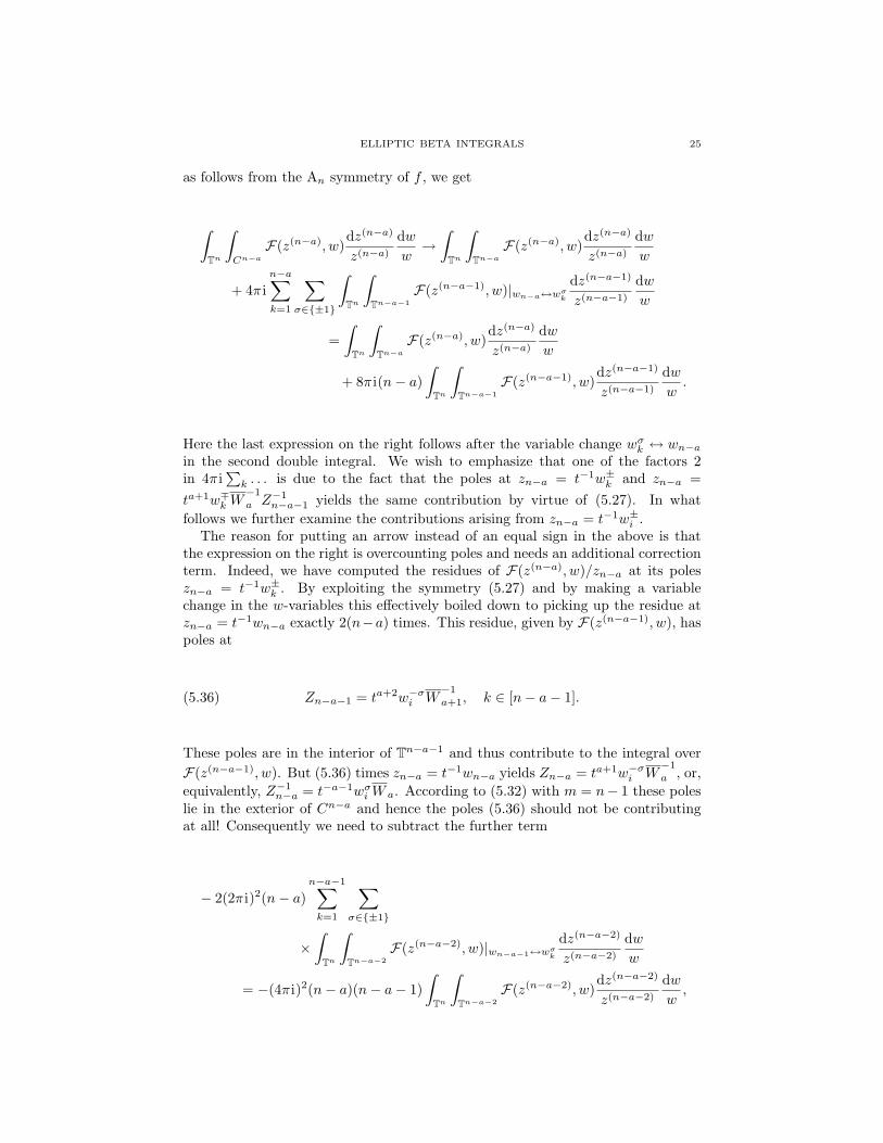
Here the last expression on the right follows after the variable change wσk ↔ wn−ain the second double integral. We wish to emphasize that one of the factors 2in 4π i

∑k . . . is due to the fact that the poles at zn−a = t−1w±k and zn−a =

ta+1w∓kW−1

a Z−1n−a−1 yields the same contribution by virtue of (5.27). In what

follows we further examine the contributions arising from zn−a = t−1w±i .The reason for putting an arrow instead of an equal sign in the above is that

the expression on the right is overcounting poles and needs an additional correctionterm. Indeed, we have computed the residues of F(z(n−a), w)/zn−a at its poleszn−a = t−1w±k . By exploiting the symmetry (5.27) and by making a variablechange in the w-variables this effectively boiled down to picking up the residue atzn−a = t−1wn−a exactly 2(n−a) times. This residue, given by F(z(n−a−1), w), haspoles at

(5.36) Zn−a−1 = ta+2w−σi W−1

a+1, k ∈ [n− a− 1].

These poles are in the interior of Tn−a−1 and thus contribute to the integral overF(z(n−a−1), w). But (5.36) times zn−a = t−1wn−a yields Zn−a = ta+1w−σi W

−1

a , or,equivalently, Z−1

n−a = t−a−1wσiW a. According to (5.32) with m = n− 1 these poleslie in the exterior of Cn−a and hence the poles (5.36) should not be contributingat all! Consequently we need to subtract the further term

− 2(2π i)2(n− a)n−a−1∑k=1

∑σ∈{±1}

×∫

Tn

∫Tn−a−2

F(z(n−a−2), w)|wn−a−1↔wσkdz(n−a−2)

z(n−a−2)

dww

= −(4π i)2(n− a)(n− a− 1)∫

Tn

∫Tn−a−2

F(z(n−a−2), w)dz(n−a−2)

z(n−a−2)

dww,

26 VYACHESLAV P. SPIRIDONOV AND S. OLE WARNAAR

where we have used the second equality in (5.27) with a → a + 2, and the An

symmetry of f . Therefore∫Tn

∫Cn−a

F(z(n−a), w)dz(n−a)

z(n−a)

dww

=∫

Tn

∫Tn−a

F(z(n−a), w)dz(n−a)

z(n−a)

dww

+ 2(4π i)(n− a)∫

Tn

∫Tn−a−1

F(z(n−a−1), w)dz(n−a−1)

z(n−a−1)

dww

+ (4π i)2(n− a)(n− a− 1)∫

Tn

∫Tn−a−2

F(z(n−a−2), w)dz(n−a−2)

z(n−a−2)

dww.

Substituting this in the left-hand side of (5.35), shifting a→ a− 1 and a→ a− 2in the sums corresponding to the integrals over Tn−a−1 and Tn−a−2 and using thebinomial identity(

n− 1a

)+ 2(n− 1a− 1

)+(n− 1a− 2

)=(n+ 1a

)=

n+ 1n− a+ 1

(n

a

)yields the wanted right-hand side of (5.35), completing the proof. �

In the integral on the right-hand side of (5.30) we make the variable changeszi → zi+a for i ∈ [n−a] followed by t−1wn−a+i → zi for i ∈ [a]. By the permutationsymmetry of f this gives

(5.37) I(x; t) =n∑a=0

(4π i)a(n

a

)(n+ 1)!

(n− a+ 1)!

×∫

Tn−a

∫(t−1T)a×Tn−a

∆(z, w(n−a), x; t)f(z)dzz

dw(n−a)

w(n−a),

with

∆(z, w(n−a), x; t) := ∆((za+1, . . . , zn), (w1, . . . , wn−a, tz1, . . . , tza), x; t)

given by the somewhat unwieldy expression

∆(z, w(n−a), x; t) =1

(p; p)a∞(q; q)a∞

∏1≤i<j≤n−a

1Γ(w±i w

±j )

(5.38)

×a∏j=1

∏n+1i=1 Γ(t2xizj , xiz−1

j )

Γ(t2z2j )∏n+1i=a+1 Γ(ziz−1

j , t2zizj)

×n−a∏i=1

∏n+1j=1 Γ(tw±i xj)

∏n+1j=a+1 Γ(t−1w±i z

−1j )

Γ(w±2i )

∏aj=1 Γ(tw±i zj)

×∏

1≤i<j≤a

1Γ(ziz−1

j , z−1i zj , t2zizj , t2zizj)

×∏

a+1≤i<j≤n+1

1Γ(ziz−1

j , z−1i zj , t2zizj , t−2z−1

i z−1j )

.

It is easily checked that the only poles of ∆(z, w(n−a), x; t) in the zj-plane locatedon the annulus 1 < |zj | < |t|−1 for j ∈ [a] are given by zj = xi for i ∈ [n].For example, the pole at zn+1 = t−1w±i p

µqν corresponds to a pole in the zj-plane (j ∈ [a]) at zj = tw±i (

∏nk=1;k 6=j zk)−1p−µq−ν with absolute value |zj | =

|t|a|p|−µ|q|−ν . For (µ, ν) = (0, 0) this implies |zj | < 1 and for (µ, ν) 6= (0, 0) this

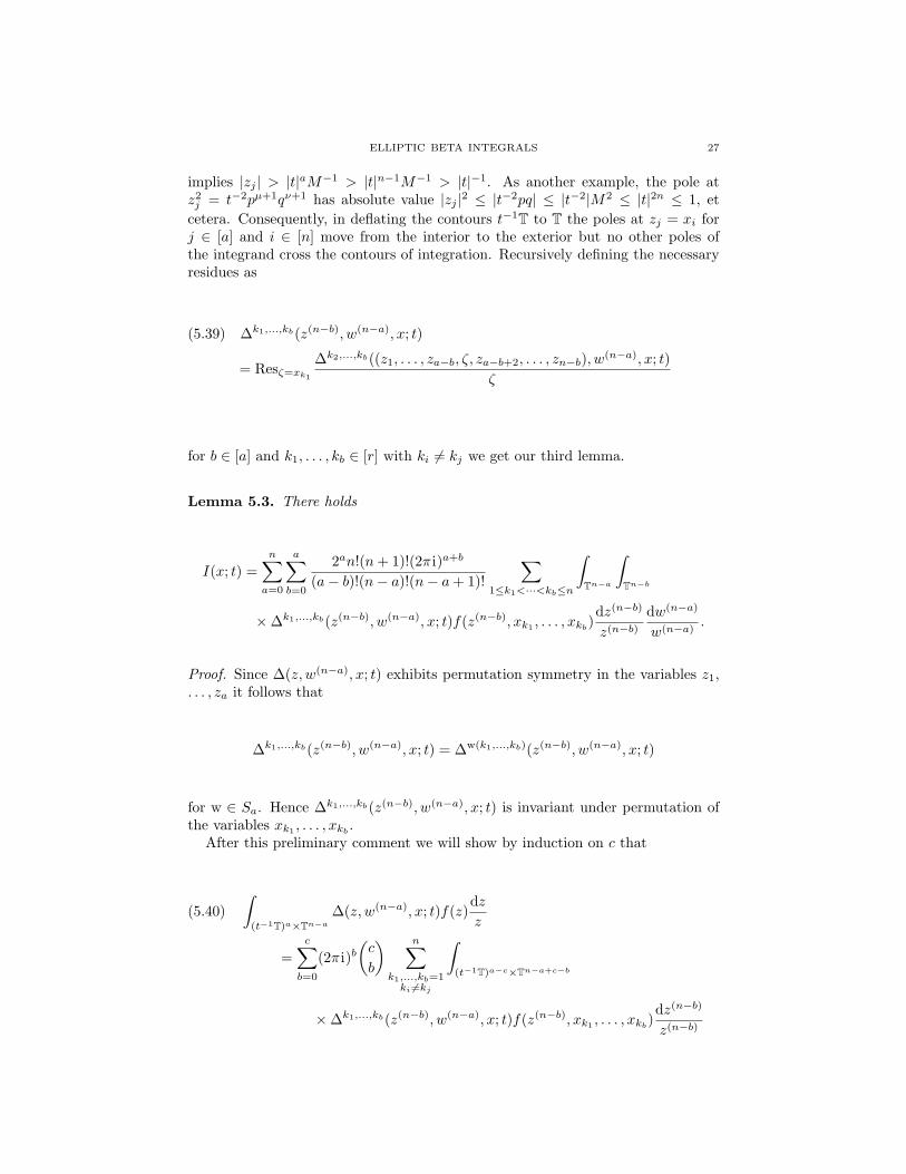
ELLIPTIC BETA INTEGRALS 27

implies |zj | > |t|aM−1 > |t|n−1M−1 > |t|−1. As another example, the pole atz2j = t−2pµ+1qν+1 has absolute value |zj |2 ≤ |t−2pq| ≤ |t−2|M2 ≤ |t|2n ≤ 1, et

cetera. Consequently, in deflating the contours t−1T to T the poles at zj = xi forj ∈ [a] and i ∈ [n] move from the interior to the exterior but no other poles ofthe integrand cross the contours of integration. Recursively defining the necessaryresidues as

(5.39) ∆k1,...,kb(z(n−b), w(n−a), x; t)

= Resζ=xk1∆k2,...,kb((z1, . . . , za−b, ζ, za−b+2, . . . , zn−b), w(n−a), x; t)

ζ

for b ∈ [a] and k1, . . . , kb ∈ [r] with ki 6= kj we get our third lemma.

Lemma 5.3. There holds

I(x; t) =n∑a=0

a∑b=0

2an!(n+ 1)!(2π i)a+b

(a− b)!(n− a)!(n− a+ 1)!

∑1≤k1<···<kb≤n

∫Tn−a

∫Tn−b

×∆k1,...,kb(z(n−b), w(n−a), x; t)f(z(n−b), xk1 , . . . , xkb)dz(n−b)

z(n−b)dw(n−a)

w(n−a).

Proof. Since ∆(z, w(n−a), x; t) exhibits permutation symmetry in the variables z1,. . . , za it follows that

∆k1,...,kb(z(n−b), w(n−a), x; t) = ∆w(k1,...,kb)(z(n−b), w(n−a), x; t)

for w ∈ Sa. Hence ∆k1,...,kb(z(n−b), w(n−a), x; t) is invariant under permutation ofthe variables xk1 , . . . , xkb .

After this preliminary comment we will show by induction on c that

(5.40)∫

(t−1T)a×Tn−a∆(z, w(n−a), x; t)f(z)

dzz

=c∑b=0

(2π i)b(c

b

) n∑k1,...,kb=1ki 6=kj

∫(t−1T)a−c×Tn−a+c−b

×∆k1,...,kb(z(n−b), w(n−a), x; t)f(z(n−b), xk1 , . . . , xkb)dz(n−b)

z(n−b)

28 VYACHESLAV P. SPIRIDONOV AND S. OLE WARNAAR

for c ∈ Za+1. Since this is trivially true for c = 0 we only need to establish theinduction step. Let L(a, c) denote the left hand side of (5.40). Then

L(a, c) =c∑b=0

(2π i)b(c

b

) n∑k1,...,kb=1ki 6=kj

∫(t−1T)a−c−1×Tn−a+c−b+1

×∆k1,...,kb(z(n−b), w(n−a), x; t)f(z(n−b), xk1 , . . . , xkb)dz(n−b)

z(n−b)

+c∑b=0

(2π i)b+1

(c

b

) n∑k0,k1,...,kb=1

ki 6=kj

∫(t−1T)a−c−1×Tn−a+c−b

×∆k0,...,kb(z(n−b−1), w(n−a), x; t)f(z(n−b−1), xk0 , . . . , xkb)dz(n−b−1)

z(n−b−1).

In the seccond sum we shift the summation index b → b + 1 and relabel the ki aski+1. By the standard binomial recurrence we then find that L(a, c) = L(a, c + 1)as desired.

To now obtain the expansion of Lemma 5.3 we choose c = a in (5.40) and usethe permutation symmetry of the integrand in the xki to justify the simplification

n∑k1,...,kb=1ki 6=kj

(. . . )→ b!∑

1≤k1<···<kb≤n

(. . . ).

Substituting the resulting expression in (5.37) completes the proof. �

By changing the order of the sums as well as the order of the integrals, theidentity of Lemma 5.3 can be rewritten as

I(x; t) =n∑b=0

∑1≤k1<···<kb≤n

n∑a=b

2an!(n+ 1)!(2π i)a+b

(a− b)!(n− a)!(n− a+ 1)!

×∫

Tn−b

[∫Tn−a

∆k1,...,kb(z(n−b), w(n−a), x; t)dw(n−a)

w(n−a)

]× f(z(n−b), xk1 , . . . , xkb)

dz(n−b)

z(n−b) .

In what may well be considered the second part of the proof of Theorem 5.2 wewill prove the following proposition.

Proposition 5.2. For b ∈ Zn and fixed 1 ≤ k1 < · · · < kb ≤ n we have

(5.41)n∑a=b

(4π i)a

(n− a+ 1)!

(n− bn− a

)∫Tn−b

[∫Tn−a

∆k1,...,kb(z(n−b), w(n−a), x; t)dw(n−a)

w(n−a)

]

× f(z(n−b), xk1 , . . . , xkb)dz(n−b)

z(n−b) = 0.

From this result it follows that the only non-vanishing contribution to I(x; t)comes from b = a = n and (k1, . . . , kn) = (1, . . . , n). As we shall see shortly,

(5.42) ∆(z(0), w(0), x; t) := ∆1,...,n(z(0), w(0), x; t) =1

(p; p)2n∞ (q; q)2n

∞,

ELLIPTIC BETA INTEGRALS 29

leading to κA κC I(x; t) = f(x) as claimed by the theorem.

Proof of Proposition 5.2. It is sufficient to prove the proposition for (k1, . . . , kb) =(1, . . . , b). Other choices of the ki (for fixed b) simply follow by a relabelling ofthe xi variables. The advantage of this particular choice of ki is that many of theexpressions below significantly simplify.

The first ingredient needed for the proof is the actual computation of

∆(z(n−b), w(n−a), x; t) := ∆1,...,b(z(n−b), w(n−a), x; t).

From definition (5.39), and the equations (5.38) and (2.6) it is not hard to showthat

∆(z(n−b), w(n−a), x; t) =1

(p; p)a+b∞ (q; q)a+b

∞

∏1≤i<j≤n−a

1Γ(w±i w

±j )

×b∏i=1

∏n+1j=b+1 Γ(x−1

i xj , t2xixj)∏n−b+1

j=1 Γ(x−1i zj , t2xizj)

a−b∏j=1

∏n+1i=b+1 Γ(t2xizj , xiz−1

j )

Γ(t2z2j )∏n−b+1i=a−b+1 Γ(ziz−1

j , t2zizj)

×n−a∏i=1

∏n+1j=b+1 Γ(tw±i xj)

∏n−b+1j=a−b+1 Γ(t−1w±i z

−1j )

Γ(w±2i )

∏a−bj=1 Γ(tw±i zj)

×∏

1≤i<j≤a−b

1Γ(ziz−1

j , z−1i zj , t2zizj , t2zizj)

×∏

a−b+1≤i<j≤n−b+1

1Γ(ziz−1

j , z−1i zj , t2zizj , t−2z−1

i z−1j )

,

where, given z(n−b),

(5.43) zn−b+1 := X−1b Z−1

n−b,

i.e., z1 · · · zn−b+1 = X−1b = x−1

1 · · ·x−1b . For b = n this implies z1 = X−1

n = xn+1

so that ∆(z(0), w(0), x; t) is given by (5.42).In the Cn elliptic elliptic beta integral (3.5) we deform Tn to Cn = C × · · · × C

with C = C−1 ⊂ C the usual positively oriented Jordan curve, such that the pointstip

µqν for i ∈ [2n + 4] are in the interior of C. With Tn replaced by such Cn

the integral (3.5) holds for all t1, . . . , t2n+4 subject only to t1 · · · t2n+4 = pq. Thenchoosing t1 · · · t2n+2 = 1 and t2n+3t2n+4 = pq and using (2.3b) and Γ(pq) = 0, weget ∫

Cn

n∏j=1

∏2n+2i=1 Γ(tiz±j )

Γ(z±2j )

∏1≤i<j≤n

1Γ(z±i z

±j )

dzz

= 0,

where Cn = C × · · · × C such that C has the points tipµqµ for i ∈ [2n + 2] in itsinterior. Replacing z by w, n by n − b, and ti → txi+b, ti+n−b+1 → t−1z−1

i fori ∈ [n− b+ 1], with zn−b+1 defined by (5.43) to ensure that

1 = t1 · · · t2n+2 → xb+1 · · ·xn+1z−11 · · · z

−1n−b+1

= xb+1 · · ·xn+1Xb = x1 · · ·xn+1 = 1,

yields, ∫Cn−b

∆(z(n−b), w(n−b), x; t)dw(n−b)

w(n−b) = 0

30 VYACHESLAV P. SPIRIDONOV AND S. OLE WARNAAR

for b ∈ Zn. Here Cn−b = C × · · · × C such that C has the points txi+bpµqν andt−1z−1

i pµqν for i ∈ [n− b+ 1] in its interior. Obviously, we then also have

(5.44)∫

Tn−b

∫Cn−b

∆(z(n−b), w(n−b), x; t)f(z(n−b), x(b))dw(n−b)

w(n−b)dz(n−b)

z(n−b) = 0,

to be compared with (5.41).Deforming Cn−b to Tn−b by successively deforming the 1-dimensional contours

C to T, the poles of the integrand at t−1z−1i (tzi) for i ∈ [n − b + 1] move from

the interior (exterior) of C to the exterior (interior) of T, but no other poles crossthe contours of integration. The function ∆(z(n−b), w(n−a), x; t) has been obtainedfrom ∆(z, w, x; t) by computing residues corresponding to poles in the z-variables,see (5.26) and (5.39). Presently we are at a stage of the calculation that requires thecomputation of residues with respect to the above-listed poles in the w-variables.Amazingly, this does not lead to a further generalization of ∆(z, w, x; t). Indeed,the following truly remarkable relation holds for a ∈ {b, . . . , n}:

(5.45) Reswn−a=t−1z−1a−b+1

∆(z(n−b), w(n−a), x; t)wn−a

= −Reswn−a=tza−b+1

∆(z(n−b), w(n−a), x; t)wn−a

= ∆(z(n−b), w(n−a−1), x; t).

Moreover, since ∆(z(n−b), w(n−a), x; t) exhibits permutation symmetry in the vari-ables za−b+1, . . . , zn−b+1 we also have

(5.46) Reswn−a=t−1z−1j

∆(z(n−b), w(n−a), x; t)wn−a

= −Reswn−a=tzj

∆(z(n−b), w(n−a), x; t)wn−a

= ∆(z(n−b), w(n−a−1), x; t)|za−b+1↔zj

for j ∈ {a− b+ 1, . . . , n− b+ 1}. These results imply our next lemma.

Lemma 5.4. For b ∈ Zn there holds

n∑a=b

(4π i)a

(n− a)!

(n− bn− a

)[∫Tn−b

+1

n− a+ 1

a−b∑c=1

∫Tc−1×(X−1

b T)×Tn−b−c

]

×∫

Tn−a∆(z(n−b), w(n−a), x; t)f(z(n−b), x(b))

dw(n−a)

w(n−a)

dz(n−b)

z(n−b) = 0.

Before proving the lemma we complete the proof of Proposition 5.2.If we can show that for all c ∈ [a − b] no poles of the integrand in the zc-plane

cross the contour of integration when X−1b T is inflated to T then the identity of

Lemma 5.4 simplifies to

n∑a=b

(4π i)a

(n− a+ 1)!

(n− bn− a

)∫Tn−b

∫Tn−a

∆(z(n−b), w(n−a), x; t)

× f(z(n−b), x(b))dw(n−a)

w(n−a)

dz(n−b)

z(n−b) = 0,

ELLIPTIC BETA INTEGRALS 31

where we divided out an overall factor (n − b + 1). Since this is (5.41) with(k1, . . . , kb) = (1, . . . , b) we are done with the proof of Proposition 5.2 if we canshow that ∆(z(n−b), w(n−a), x; t) is free of poles in the annulus |Xb|−1 ≤ |zj | ≤ 1 forj ∈ [a− b]. Since ∆(z(n−b), w(n−a), x; t) has permutation symmetry in the variablesz1, . . . , za−b, it is enough to check this condition for j = a−b. The rest is a matter ofcase-checking, where it should be noted that, since b ≤ n−1, |t|n−1 ≤ |t|b < |Xb|−1.For example, the pole at za−b = t−2x−1

i+bp−µq−ν (for i ∈ [n − b + 1]) has absolute

value |za−b| > |t|−1 > 1 for i 6= n − b + 1 and absolute value |za−b| > |t|−n−2 > 1for i = n − b + 1. The pole at za−b = xip

µqν (for i = b + 1, . . . , n + 1) hasabsolute value |za−b| > |t|−1 > 1 if (µ, ν) = (0, 0) and i 6= n + 1, has absolutevalue |za−b| = |xn+1| < |Xb|−1 if (µ, ν) = (0, 0) and i = n + 1, has absolute value|za−b| < |t|−1M < |t|n−1 < |Xb|−1 if (µ, ν) 6= (0, 0) and i 6= n+ 1, and has absolutevalue |za−b| < M < |t|n < |Xb|−1 if (µ, ν) 6= (0, 0) and i = n+ 1. �

Proof of Lemma 5.4. We will show by induction on d that for b ∈ Zn and d ∈{b, . . . , n} there holds

Lb,d :=d∑a=b

(4π i)a

(d− a)!

(n− bn− a

)[∫Tn−b

+1

n− a+ 1

a−b∑c=1

∫Tc−1×(X−1

b T)×Tn−b−c

]

×∫

Td−a×Cn−da

∆(z(n−b), w(n−a), x; t)f(z(n−b), x(b))dw(n−a)

w(n−a)

dz(n−b)

z(n−b) = 0.

Here Cn−da = Ca × · · · × Ca with Ca a contour that has the points

txi+bpµqν for i ∈ [n− b+ 1],(5.47a)

t−1z−1i+a−bp

µqν for i ∈ [n− a+ 1],(5.47b)

t−1zipµ+1qν+1 for i ∈ [a− b],(5.47c)

in its interior. Since for d = b we recover (5.44) it suffices to establish that Lb,d =(d− b+ 1)Lb,d+1 for d ∈ {b, . . . , n− 1}.

Without loss of generality we may assume that |t|2n+1 < |Ca| < |t|−2n−1. Thisis compatible with the fact that the points listed in (5.47a) and (5.47b) must liein the interior of Ca, and guarantees that the points listed in (5.47c) lie in itsinterior. When integrating over w(n−a) for fixed z(n−b) we may also assume thatza−b+1, . . . , zn−b+1 are all distinct.

We now deform Cn−da to Cn−d−1a × T. The poles of ∆(z(n−b), w(n−a), x; t) in

the wn−a-plane coincide with the points listed in (5.47) and their reciprocals. Theusual inspection of their moduli shows that under the assumption that |xi| < |t|−1,the only poles crossing the contour are those corresponding to wn−a = t−1z−1

k+a−bfor k ∈ [n− a+ 1]. Hence, by (5.45) and (5.46),

Ia,d(z(n−b), x; t) :=∫

Td−a×Cn−da

∆(z(n−b), w(n−a), x; t)dw(n−a)

w(n−a)

(5.48)

= Ia,d+1(z(n−b), x; t)

+ 4π in−b+1∑k=a−b+1

∫Td−a×Cn−d−1

a;k

∆(z(n−b), w(n−a−1), x; t)|za−b+1↔zkdw(n−a−1)

w(n−a−1).

32 VYACHESLAV P. SPIRIDONOV AND S. OLE WARNAAR

Here the integration variables wd−a+1 and wn−a in the first integral on the righthave been permuted in order to simplify Td−a ×Cn−d−1

a ×T to Td−a+1 ×Cn−d−1a ,

leading to Ia,d+1. Furthermore, Cn−d−1a;k = Ca;k × · · · × Ca;k with Ca;k a contour

that has the points listed in (5.47) in its interior be it that in (5.47b) and (5.47c)the respective conditions i 6= k and i = k need to be added. This latter conditionis automatically satisfied if we demand that |t|2n+1 < |Ca;k| < |t|−2n−1 which alsoimplies that Ca;a−b+1 may be identified with Ca+1 so that Cn−d−1

a;a−b+1 = Cn−d−1a+1 .

Next consider

Ja,b,d :=∫

Tn−bIa,d(z(n−b), x; t)f(z(n−b), x(b))

dz(n−b)

z(n−b)(5.49a)

and

Ka,b,c,d :=∫

Tc−1×(X−1b T)×Tn−b−c

Ia,d(z(n−b), x; t)f(z(n−b), x(b))dz(n−b)

z(n−b) .(5.49b)

We will compute these integrals using (5.48), starting with Ja,b,d. By permutingthe integration variables zk and za−b+1 for k ∈ {a − b + 1, . . . , n − b}, and byusing the permutation symmetry of f , the sum over k in (5.48) (with the termk = n− b+ 1 excluded) simply gives rise to (n− a) times Ja+1,b,d+1. The last termin the sum is to be treated somewhat differently. Recalling the definition of zn−b+1

in (5.43) we make the variable change za−b+1 ↔ zn−b+1 = Z−1n−bX

−1b in the integral

corresponding to this remaining term. By the An symmetry of f this leaves theintegrand unchanged. Consequently,

(5.50) Ja,b,d = Ja,b,d+1 + 4π i(n− a)Ja+1,b,d+1 + 4π iKa+1,b,a−b+1,d+1.

We carry out exactly the same variables changes to compute Ka,b,c,d for c ∈ [a− b].Note that since c ≤ a − b these changes do not interfere with the structure ofthe contours of (5.49b). The only notable difference will be that when permutingza−b+1 ↔ zn−b+1 = Z−1

n−bX−1b corresponding to the last term in the sum over

k in (5.48), the za−b+1 contour of integration will not change from T to X−1b T

as before, but will remain just T. Indeed, when za−b+1 → X−1b Z−1

n−b we find|za−b+1| → |X−1

b Z−1n−b| = 1 since |zc| = |X−1

b |. Therefore

(5.51) Ka,b,c,d = Ka,b,c,d+1 + 4π i(n− a+ 1)Ka+1,b,c,d+1.

The remainder of the proof is elementary. By definition,

Lb,d =d∑a=b

(4π i)a

(d− a)!

(n− bn− a

)[Ja,b,d +

1n− a+ 1

a−b∑c=1

Ka,b,c,d

].

Substituting (5.50) and (5.51) and shifting the summation index from a to a − 1in all terms of the summand that carry the subscript a + 1 yields Lb,d = (d − b +1)Lb,d+1. �

6. Alternative proof of the new An elliptic beta integral

The proof of Theorem 5.3 presented in this section adopts and refines a techniquefor proving elliptic beta integrals via q-difference equations that was recently devel-oped in [26]. We note that this method is different from the q-difference approachof Gustafson [11]. The latter employs q-difference equations depending solely onthe “external” parameters in beta integrals (like the ti and si in (3.4) and (3.5))

ELLIPTIC BETA INTEGRALS 33

and not on the integration variables themselves. Although Gustafson’s method canalso be applied to the integral of Theorem 5.3 by virtue of the fact that both sidesof the integral identity satisfy

n+1∑i=1

θ(q−1Ss−1i s−1

n+2)θ(Ss−1

n+2s−1n+3)

n+1∏j=1j 6=i

θ(q−1s−1j sn+3)

θ(sis−1j )

× I(s1, . . . , si−1, qsi, si+1, . . . , sn+2, q−1sn+3) = I(s1, . . . , sn+3),

the proof would require a non-trivial vanishing hypothesis similar to those formu-lated in [7].

After these preliminary remarks we turn our attention to the actual proof ofTheorem 5.3. We begin by noting that the kernel ρ(z; s, t) defined in (5.20) satisfiesa q-difference equation involving the integration variables. For v = (v1, . . . , vn) ∈Cn and a ∈ C let πi,a(v) = (v1, . . . , vi−1, avi, vi+1, . . . , vn).

Lemma 6.1. We have

(6.1) ρ(z; s, t)− ρ(z; s, π1,q(t)) =n∑i=1

[gi(z; s, t)− gi(πi,q−1(z); s, t)

],

where gi(z; s, t) = ρ(z; s, t)fi(z; s, t) and

(6.2) fi(z; s, t) = t1zn+1θ(St21)n∏j=1

θ(t1zj)θ(zjz−1

n+1, Stjz−1n+1)

n∏j=2

θ(tjzi, q−1Stjz−1i )

θ(q−1tjzn+1)

×n+3∏j=1

θ(sjz−1n+1)

θ(t1sj)

n∏j=1j 6=i

θ(q−1z−1j zn+1, Sz

−1j z−1

n+1)

θ(ziz−1j , q−1Sz−1

i z−1j )

.

Proof. From (2.4) and θ(x) = −x θ(x−1) it readily follows that

ρ(z; s, π1,q(t))ρ(z; s, t)

=n+1∏i=1

θ(t1zi)θ(St1z−1

i )

n+3∏j=1

θ(St1s−1j )

θ(t1sj)

and

ρ(πi,q−1(z); s, t)ρ(z; s, t)

= −ziθ(q−2ziz

−1n+1)

qzn+1θ(z−1i zn+1)

n∏j=1

θ(tjzn+1, q−1Stjz

−1n+1)

θ(q−1tjzi, Stjz−1i )

×n+3∏j=1

θ(sjz−1i )

θ(q−1sjz−1n+1)

n∏j=1j 6=i

θ(q−1ziz−1j , q−1zjz

−1n+1, Sz

−1i z−1

j )

θ(z−1i zj , z

−1j zn+1, q−1Sz−1

j z−1n+1)

.

34 VYACHESLAV P. SPIRIDONOV AND S. OLE WARNAAR

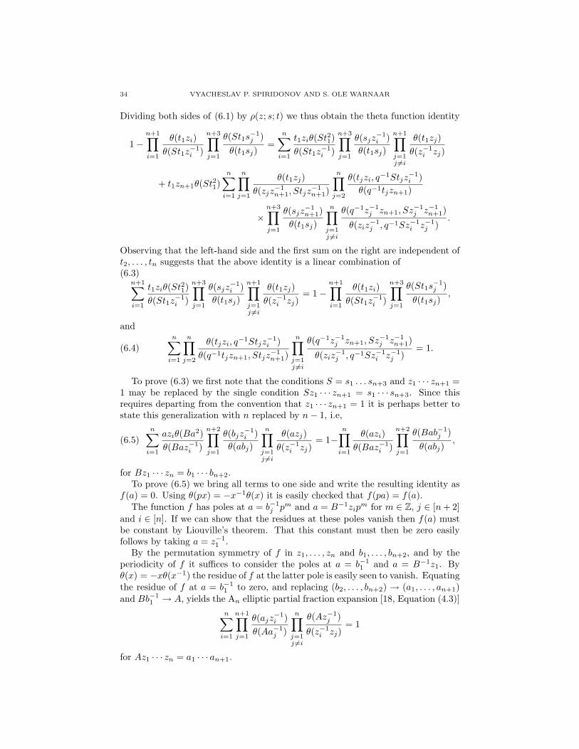
Dividing both sides of (6.1) by ρ(z; s; t) we thus obtain the theta function identity

1−n+1∏i=1

θ(t1zi)θ(St1z−1

i )

n+3∏j=1

θ(St1s−1j )

θ(t1sj)=

n∑i=1

t1ziθ(St21)θ(St1z−1

i )

n+3∏j=1

θ(sjz−1i )

θ(t1sj)

n+1∏j=1j 6=i

θ(t1zj)θ(z−1

i zj)

+ t1zn+1θ(St21)n∑i=1

n∏j=1

θ(t1zj)θ(zjz−1

n+1, Stjz−1n+1)

n∏j=2

θ(tjzi, q−1Stjz−1i )

θ(q−1tjzn+1)

×n+3∏j=1

θ(sjz−1n+1)

θ(t1sj)

n∏j=1j 6=i

θ(q−1z−1j zn+1, Sz

−1j z−1

n+1)

θ(ziz−1j , q−1Sz−1

i z−1j )

.

Observing that the left-hand side and the first sum on the right are independent oft2, . . . , tn suggests that the above identity is a linear combination of(6.3)

n+1∑i=1

t1ziθ(St21)θ(St1z−1

i )

n+3∏j=1

θ(sjz−1i )

θ(t1sj)

n+1∏j=1j 6=i

θ(t1zj)θ(z−1

i zj)= 1−

n+1∏i=1

θ(t1zi)θ(St1z−1

i )

n+3∏j=1

θ(St1s−1j )

θ(t1sj),

and

(6.4)n∑i=1

n∏j=2

θ(tjzi, q−1Stjz−1i )

θ(q−1tjzn+1, Stjz−1n+1)

n∏j=1j 6=i

θ(q−1z−1j zn+1, Sz

−1j z−1

n+1)

θ(ziz−1j , q−1Sz−1

i z−1j )

= 1.

To prove (6.3) we first note that the conditions S = s1 . . . sn+3 and z1 · · · zn+1 =1 may be replaced by the single condition Sz1 · · · zn+1 = s1 · · · sn+3. Since thisrequires departing from the convention that z1 · · · zn+1 = 1 it is perhaps better tostate this generalization with n replaced by n− 1, i.e,

(6.5)n∑i=1

aziθ(Ba2)θ(Baz−1

i )

n+2∏j=1

θ(bjz−1i )

θ(abj)

n∏j=1j 6=i

θ(azj)θ(z−1

i zj)= 1−

n∏i=1

θ(azi)θ(Baz−1

i )

n+2∏j=1

θ(Bab−1j )

θ(abj),

for Bz1 · · · zn = b1 · · · bn+2.To prove (6.5) we bring all terms to one side and write the resulting identity as

f(a) = 0. Using θ(px) = −x−1θ(x) it is easily checked that f(pa) = f(a).The function f has poles at a = b−1

j pm and a = B−1zipm for m ∈ Z, j ∈ [n+ 2]

and i ∈ [n]. If we can show that the residues at these poles vanish then f(a) mustbe constant by Liouville’s theorem. That this constant must then be zero easilyfollows by taking a = z−1

1 .By the permutation symmetry of f in z1, . . . , zn and b1, . . . , bn+2, and by the

periodicity of f it suffices to consider the poles at a = b−11 and a = B−1z1. By

θ(x) = −xθ(x−1) the residue of f at the latter pole is easily seen to vanish. Equatingthe residue of f at a = b−1

1 to zero, and replacing (b2, . . . , bn+2) → (a1, . . . , an+1)and Bb−1

1 → A, yields the An elliptic partial fraction expansion [18, Equation (4.3)]n∑i=1

n+1∏j=1

θ(ajz−1i )

θ(Aa−1j )

n∏j=1j 6=i

θ(Az−1j )

θ(z−1i zj)

= 1

for Az1 · · · zn = a1 · · · an+1.

ELLIPTIC BETA INTEGRALS 35

The task of proving (6.4) is even simpler. From [9, Lemma 4.14] we have theelliptic partial fraction expansion

n∑i=1

n−1∏j=1

θ(bjzi, bjz−1i )

θ(abj , a−1bj)

n∏j=1j 6=i

θ(azj , a−1zj)θ(z−1

i zj , zizj)= 1.

Making the substitutions

zi → q−1/2S1/2z−1i , bj → q−1/2S1/2tj , a→ q−1/2S−1/2zn+1

results in (6.4). �

By integrating the identity of Lemma 6.1 over Tn and by rescaling some of theintegration variables, we obtain

(6.6) I(s, t)− I(s, π1,q(t)) = κAn∑i=1

(∫Tn−∫

Ti−1×(q−1T)×Tn−i

)gi(z; s, t)

dzz,

where I(s, t) denotes the integral on the left of (5.19). A careful inspection learnsthat gi(z; s, t) has poles in the zi-plane at

zi =

Sz−1

j pµqν−1

Stjp−µ−1q−ν−2+δj,1

t−1j p−µq−ν−1

sjpµqν

, zn+1 =

Sz−1

j pµqν+1 j ∈ [n]/{i}Stjp

−µ−1q−ν j ∈ [n]t−1j p−µq1−ν−δj,1 j ∈ [n]sjp

µqν+1 j ∈ [n+ 3],

where zn+1 = a stands for z−1i = az1 · · · zi−1zi+1 · · · zn. Imposing the conditions

(which are stronger than (5.15))

(6.7) max{|t1|, |q−1t2|, . . . , |q−1tn|, |s1|, . . . , |sn+3|,|pS−1t−1

1 |, . . . , |pS−1t−1n |, |q−1S|} < 1

it follows that none of the listed poles of gi lies on the annulus 1 ≤ |zi| ≤ |q|−1.Consequently, when (6.7) holds the right-hand side of (6.6) vanishes and

(6.8) I(s, t) = I(s, π1,q(t)).

Expanding I(s, t) in a Taylor series in p we have

(6.9) I(s, t; q, p) =∞∑j=0

Ij(s, t; q)pj ,

with Ij(s, t; q) holomorphic in s and t for

max{|t1|, . . . , |tn|, |s1|, . . . , |sn+3|} < 1.

(The remaining conditions of (5.15) involving the parameter p ensure convergenceof the series (6.9), but, obviously, bear no relation to the analyticity of Ij(s, t; q).)

Thanks to (6.8) we have the termwise q-difference Ij(s, t; q) = Ij(s, π1,q(t)) when

max{|t1|, |q−1t2|, . . . , |q−1tn|, |s1|, . . . , |sn+3|, |q−1S|} < 1.

Since this may be iterated and since the limiting point t1 = 0 of the sequencet1, t1q, t1q

2, . . . lies inside the domain of analyticity of Ij(s, t), we conclude that

36 VYACHESLAV P. SPIRIDONOV AND S. OLE WARNAAR

Ij(s, t) is independent of t1. Lifting this to I(s, t) and exploiting the symmetry inthe ti it follows that I(s, t) is independent of t for

max{|q−1t1|, . . . , |q−1tn|, |s1|, . . . , |sn+3|, |pS−1t−11 |, . . . , |pS−1t−1

n |, |q−1S|} < 1

and thus, by analytic continuation, for (5.15).In order to compute I(s, t) = I(s) we repeat the reasoning of Section 5.2 and

note that when (5.15) is replaced by (5.25) then I(s) is given by the integral on theleft of (5.22). We also know that this integral does not depend on t and hence, by(5.24),

I(s) = limti→s−1

i

∀ i∈[n]

I(s) = κA limti→s−1

i

∀ i∈[n]

∑λ

ρλ(s, t).

The expression on the right equals to 1 thanks to the trivial fact that for Ni = 0we have λ = 0 and the conditions ti = s−1

i yield κA ρ0(s, t) = 1. As a final remark,we note that application of the full residue calculus with Ni 6= 0 to our An integralresults in Theorems 5.5 and 5.6. Therefore, the considerations of the present sectionprovide an alternative proof of the corresponding sums as well.

References

1. G. E. Andrews, Multiple series Rogers–Ramanujan type identities, Pacific J. Math. 114

(1984), 267–283. 1

2. G. E. Andrews, Bailey’s transform, lemma, chains and tree, Special Functions 2000: CurrentPerspective and Future Directions (Kluwer Academic Publishers, Dordrecht, 2001), pp. 1–22.

1

3. G. E. Andrews, R. Askey, and R. Roy, Special Functions, Encyclopedia of Math. Appl. 71,Cambridge Univ. Press, Cambridge, 1999. 1

4. R. Askey and J. Wilson, Some basic hypergeometric orthogonal polynomials that generalize

Jacobi polynomials, Mem. Amer. Math. Soc. 54 (1985), no. 319. 15. G. Bhatnagar, Dn basic hypergeometric series, Ramanujan J. 3 (1999), 175–203. 5.2.2

6. J. F. van Diejen and V. P. Spiridonov, An elliptic Macdonald–Morris conjecture and multiple

modular hypergeometric sums, Math. Res. Lett. 7 (2000), 729–746. 1, 2, 5.2.27. J. F. van Diejen and V. P. Spiridonov, Elliptic Selberg integrals, Internat. Math. Res. Notices

20 (2001), 1083–1110. 1, 2, 3, 68. J. F. van Diejen and V. P. Spiridonov, Unit circle elliptic beta integrals, Ramanujan J. 10

(2005), 187–204. 1

9. R. A. Gustafson, Multilateral summation theorems for ordinary and basic hypergeometricseries in U(n), SIAM J. Math. Anal. 18 (1987), 1576–1596. 6

10. R. A. Gustafson, A generalization of Selberg’s beta integral, Bull. Amer. Math. Soc. (N.S.) 22

(1990), 97–105. 111. R. A. Gustafson, Some q-beta and Mellin–Barnes integrals with many parameters associated

to the classical groups, SIAM J. Math. Anal. 23 (1992), 525–551. 1, 3, 5.2.1, 5.2.1, 6

12. R. A. Gustafson, Some q-beta integrals on SU(n) and Sp(n) that generalize the Askey-Wilsonand Nassrallah-Rahman integrals, SIAM J. Math. Anal. 25 (1994), 441–449. 1

13. R. A. Gustafson and M. A. Rakha, q-Beta integrals and multivariate basic hypergeometric

series associated to root systems of type Am, Ann. Comb. 4 (2000), 347–373. 114. V. B. Kuznetsov and E. K. Sklyanin, Separation of variables and integral relations for special

functions, Ramanujan J. 3 (1999), 5–35. 4.215. B. Nassrallah and M. Rahman, Projection formulas, a reproducing kernel and a generating

function for q-Wilson polynomials, SIAM J. Math. Anal. 16 (1985), 186–197. 1, 3

ELLIPTIC BETA INTEGRALS 37

16. M. Rahman, An integral representation of a 10ϕ9 and continuous bi-orthogonal 10ϕ9 rational

functions, Canad. J. Math. 38 (1986), 605–618. 1, 3

17. E. M. Rains, Transformations of elliptic hypergeometric integrals, Ann. of Math. (2) 171(2010), 169–243. 1, 3, 3

18. H. Rosengren, Elliptic hypergeometric series on root systems, Adv. Math. 181 (2004), 417–

447. 5.2.2, 619. S. N. M. Ruijsenaars, First order analytic difference equations and integrable quantum sys-

tems, J. Math. Phys. 38 (1997), 1069–1146. 2

20. M. Schlosser, Multidimensional matrix inversions and Ar and Dr basic hypergeometric series,Ramanujan J. 1 (1997), 243–274. 5.2.2

21. A. Selberg, Bemerkninger om et multipelt integral, Norske Mat. Tidsskr. 26 (1944), 71–78. 1

22. V. P. Spiridonov, On the elliptic beta function, Russian Math. Surveys 56 (2001), 185–186.1, 3

23. V. P. Spiridonov, An elliptic incarnation of the Bailey chain, Int. Math. Res. Notices. 37(2002), 1945–1977. 1

24. V. P. Spiridonov, Theta hypergeometric integrals, Algebra i Analiz 15 (2003), 161–215 (St.

Petersburg Math. J. 15 (2004), 929–967). 1, 2, 3, 5.2.225. V. P. Spiridonov, A Bailey tree for integrals, Theor. Math. Phys. 139 (2004), 536–541. 1, 4.2

26. V. P. Spiridonov, Short proofs of the elliptic beta integrals, Ramanujan J. 13 (2007), 265–283.

1, 3, 3, 627. S. O. Warnaar, 50 Years of Bailey’s lemma, Algebraic Combinatorics and Applications

(Springer, Berlin, 2001), pp. 333–347. 1

28. S. O. Warnaar, Summation and transformation formulas for elliptic hypergeometric series,Constr. Approx. 18 (2002), 479–502. 2

29. S. O. Warnaar, Extensions of the well-poised and elliptic well-poised Bailey lemma, Indag.

Math. (N.S.) 14 (2003), 571–588. 1

Bogoliubov Laboratory of Theoretical Physics, JINR, Dubna, Moscow Region 141980,

Russia and Max–Planck–Institut fur Mathematik, Vivatsgasse 7, D-53111, Bonn, Ger-

many

Department of Mathematics and Statistics, The University of Melbourne, VIC 3010,

Australia