Congressional Budget Office

Investigating Monte Carlo Variation in a Dynamic Microsimulation Model

Presentation to the Fifth World Congress of the International Microsimulation Association (IMA)

September 2, 2015

Michael Simpson

Principal Analyst, Health, Retirement, and Long-Term Analysis Division

1 CO NGRES S IO NA L BUDGE T O F F IC E

Dynamic Microsimulation

■ Microsimulation: a simulation model that operates on individual units (people, firms, vehicles . . .).

■ Dynamic: moving forward in time, with each period based on the outcome of the last.

■ CBO’s long term model, CBOLT, is a dynamic microsimulation model for the United States with individual demographic, labor, and Old-Age, Survivors, and Disability Insurance (OASDI) processes combined with a Solow growth model.

2 CO NGRES S IO NA L BUDGE T O F F IC E

Random Numbers in Dynamic Microsimulation

■ Random numbers are used to determine individuals’ outcomes in at least one, but often many more, model processes.

■ In each process, a modeled probability is compared with a random number to determine the process’s outcome for each individual simulated.

■ Processes based on random numbers and probabilities are called stochastic.

3 CO NGRES S IO NA L BUDGE T O F F IC E

Stochastic Processes in CBOLT

■ Emigration

■ Marriage

■ Divorce

■ Fertility

■ Health status

■ Mortality

■ Educational attainment

■ Labor force participation

■ Earnings

■ Disability incidence

■ Disability recovery

■ Retirement (claiming)

4 CO NGRES S IO NA L BUDGE T O F F IC E

Monte Carlo Variation and Error

■ Outcomes of stochastic processes vary and depend on the random numbers that are drawn.

■ Because different sets of random numbers produce different outcomes, microsimulation models exhibit variation that depends only on the draw of random numbers.

■ That variation, which is called Monte Carlo variation, can lead to problems in the interpretation and presentation of microsimulation results.

5 CO NGRES S IO NA L BUDGE T O F F IC E

Example: Fertility

■ There are 2.256 million 25-year-old women in the United States, and they have a 9.4 percent average probability of having a child.

■ For this example, assume a 1/1000 sample, so there are 2,256 representative individuals (women) in the model.

■ In a nonmicro model, the number of children born would be the number of women in the group times the group probability.

■ In a simple microsimulation, a random number is drawn for each individual, and a child is assigned to that individual if the random number is lower than the individual’s probability of having a child.

6 CO NGRES S IO NA L BUDGE T O F F IC E

Distribution of Number of Children After 1,000 Runs of a Simple Microsimulation

■ In a nonmicro model: 2,256 women × 9.4 percent = 212 children

0

5

10

15

20

25

30

35

40

170 180 190 200 210 220 230 240 250Number of Children

Number of Simulations

7 CO NGRES S IO NA L BUDGE T O F F IC E

Small Changes Matter in a Dynamic Microsimulation

■ In a dynamic model, outcomes each year are based on the model’s outcomes for the prior year.

■ Changes propagate in later years in many ways.

– Larger birth cohorts go on to have more children (on average).

– Larger birth cohorts mean more workers, greater economic output, and eventually more Social Security spending.

– Labor supply differs for mothers with children at home, which leads to different hours, earnings, and output.

– Probabilities are a function of the state of the model, so different earnings, wages, etc. mean that individuals’ outcomes will change even when the same random numbers are used.

8 CO NGRES S IO NA L BUDGE T O F F IC E

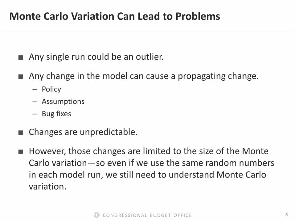
Monte Carlo Variation Can Lead to Problems

■ Any single run could be an outlier.

■ Any change in the model can cause a propagating change.

– Policy

– Assumptions

– Bug fixes

■ Changes are unpredictable.

■ However, those changes are limited to the size of the Monte Carlo variation—so even if we use the same random numbers in each model run, we still need to understand Monte Carlo variation.

9 CO NGRES S IO NA L BUDGE T O F F IC E

How Large Is the Monte Carlo Variation (and the Error)?

■ Cannot be computed mathematically

■ Determined empirically by Monte Carlo simulation using varying random numbers

■ Different for different outcomes

■ Generally small in comparison with the outcomes, but often not small in comparison with a proposed policy change

10 CO NGRES S IO NA L BUDGE T O F F IC E

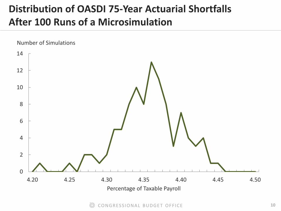
Distribution of OASDI 75-Year Actuarial Shortfalls After 100 Runs of a Microsimulation

0

2

4

6

8

10

12

14

4.20 4.25 4.30 4.35 4.40 4.45 4.50

Percentage of Taxable Payroll

Number of Simulations

11 CO NGRES S IO NA L BUDGE T O F F IC E

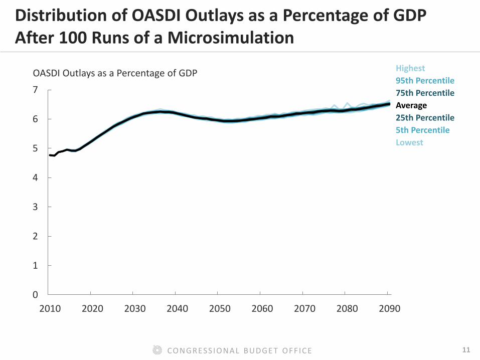
Distribution of OASDI Outlays as a Percentage of GDP After 100 Runs of a Microsimulation

0

1

2

3

4

5

6

7

2010 2020 2030 2040 2050 2060 2070 2080 2090

OASDI Outlays as a Percentage of GDP

Lowest

Highest

5th Percentile

95th Percentile

75th Percentile

25th Percentile

Average

12 CO NGRES S IO NA L BUDGE T O F F IC E

Distribution of OASDI Outlays as a Percentage of GDP After 100 Runs of a Microsimulation: A Closer Look

4.7

4.9

5.1

5.3

5.5

5.7

5.9

6.1

6.3

6.5

6.7

2010 2020 2030 2040 2050 2060 2070 2080 2090

OASDI Outlays as a Percentage of GDP

Lowest

Highest

5th Percentile

95th Percentile

75th Percentile

25th Percentile

Average

13 CO NGRES S IO NA L BUDGE T O F F IC E

Distribution of Differences From the Average in OASDI Outlays as a Percentage of GDP After 100 Runs of a Microsimulation

-2

-1

0

1

2

3

4

5

2010 2020 2030 2040 2050 2060 2070 2080 2090

Percentage Difference From Average of 100 Runs

Lowest

Highest

5th Percentile

95th Percentile

75th Percentile

25th Percentile

14 CO NGRES S IO NA L BUDGE T O F F IC E

-2

-1

0

1

2

3

4

5

6

7

2010 2020 2030 2040 2050 2060 2070 2080 2090

Effect on OASDI Outlays as a Percentage of GDP From a Change of One Death in 2015, Single Run

■ Perturb the model a tiny amount—in this case, by just a single death in 2015 out of more than 2700 representative deaths—and changes propagate in later years.

Percent

Base Case

Change of One Death

Percentage Difference

15 CO NGRES S IO NA L BUDGE T O F F IC E

-2

-1

0

1

2

3

4

5

6

7

2010 2020 2030 2040 2050 2060 2070 2080 2090

Effect on OASDI Outlays as a Percentage of GDP From a Change of One Death in 2015

■ The changes are the same size as the Monte Carlo variation.

Percent Base Case (Single run)

Change of One Death (Single run)

5th Percentile of the Monte Carlo Distribution (100 runs)

95th Percentile of the Monte Carlo Distribution (100 runs)

Single Run

Percentage Difference

16 CO NGRES S IO NA L BUDGE T O F F IC E

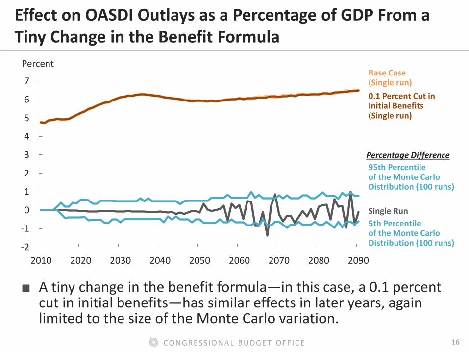
Effect on OASDI Outlays as a Percentage of GDP From a Tiny Change in the Benefit Formula

■ A tiny change in the benefit formula—in this case, a 0.1 percent cut in initial benefits—has similar effects in later years, again limited to the size of the Monte Carlo variation.

-2

-1

0

1

2

3

4

5

6

7

2010 2020 2030 2040 2050 2060 2070 2080 2090

Percent Base Case (Single run)

0.1 Percent Cut in Initial Benefits (Single run)

5th Percentile of the Monte Carlo Distribution (100 runs)

95th Percentile of the Monte Carlo Distribution (100 runs)

Single Run

Percentage Difference

17 CO NGRES S IO NA L BUDGE T O F F IC E

What Can Be Done? What Have We Done?

■ Increase sample size

■ Use targets from macro models to guide the microsimulation

■ Pick a baseline run that has important values close to the center of the Monte Carlo distribution

■ Average among many simulations that use different random numbers

18 CO NGRES S IO NA L BUDGE T O F F IC E

Increase Sample Size

■ Increases memory requirements and computational time

■ The additional data necessary may not be available

19 CO NGRES S IO NA L BUDGE T O F F IC E

Use Targets From Macro Models to Guide the Microsimulation

■ Uses random numbers combined with modeled probabilities to rank individuals; then selects the highest-ranked individuals until a macro-derived target is reached

■ Typically used to keep the simulation on track over longer periods of time

■ Does not eliminate Monte Carlo variation! Because characteristics vary among the individuals in the model, the random numbers still matter to outcomes

■ Used in CBOLT for various processes, such as the mortality-process example shown earlier

20 CO NGRES S IO NA L BUDGE T O F F IC E

Pick a Baseline Run That Has Important Values Close to the Center of the Monte Carlo Distribution

■ Easy to do if the model is built to select one of the Monte Carlo runs

■ Avoids a very likely move back toward the center of distribution with perturbation of the model if the baseline run were to be an outlier

21 CO NGRES S IO NA L BUDGE T O F F IC E

Distribution of OASDI 75-Year Actuarial Shortfalls After 100 Runs of a Microsimulation

0

2

4

6

8

10

12

14

4.20 4.25 4.30 4.35 4.40 4.45 4.50

Percentage of Taxable Payroll

Number of Simulations

Selected Single-Run Baseline

22 CO NGRES S IO NA L BUDGE T O F F IC E

Average Among Many Simulations That Use Different Random Numbers

■ May be used when more precision is needed

■ Effective in reducing error

■ No increased memory or additional data needed

■ Increases computing time

■ Need to determine reasonable number of runs, which is a trade-off between error and the time that the modeling takes

23 CO NGRES S IO NA L BUDGE T O F F IC E

Effect on OASDI Outlays as a Percentage of GDP From a Change of One Death in 2015

■ Change one death in 2015, and costs can differ by +/- 1 percent.

-2

-1

0

1

2

3

4

5

6

7

2010 2020 2030 2040 2050 2060 2070 2080 2090

Base Case (Single run)

Change of One Death (Single run)

5th Percentile of the Monte Carlo Distribution (100 runs)

95th Percentile of the Monte Carlo Distribution (100 runs)

Single Run

Percent

Percentage Difference

24 CO NGRES S IO NA L BUDGE T O F F IC E

Effect on OASDI Outlays as a Percentage of GDP From a Change of One Death in 2015, Averaging Among Runs

■ Change one death in 2015, but do 30 Monte Carlo runs; variation is reduced greatly.

-2

-1

0

1

2

3

4

5

6

7

2010 2020 2030 2040 2050 2060 2070 2080 2090

Base Case (Average of 30 runs)

Change of One Death (Average of 30 runs)

5th Percentile of the Monte Carlo Distribution (100 runs)

95th Percentile of the Monte Carlo Distribution (100 runs)

Average of 30 Runs

Percent

Percentage Difference

25 CO NGRES S IO NA L BUDGE T O F F IC E

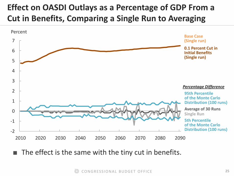
Effect on OASDI Outlays as a Percentage of GDP From a Cut in Benefits, Comparing a Single Run to Averaging

■ The effect is the same with the tiny cut in benefits.

-2

-1

0

1

2

3

4

5

6

7

2010 2020 2030 2040 2050 2060 2070 2080 2090

Base Case (Single run)

0.1 Percent Cut in Initial Benefits (Single run)

5th Percentile of the Monte Carlo Distribution (100 runs)

95th Percentile of the Monte Carlo Distribution (100 runs)

Average of 30 Runs

Percent

Single Run

Percentage Difference

26 CO NGRES S IO NA L BUDGE T O F F IC E

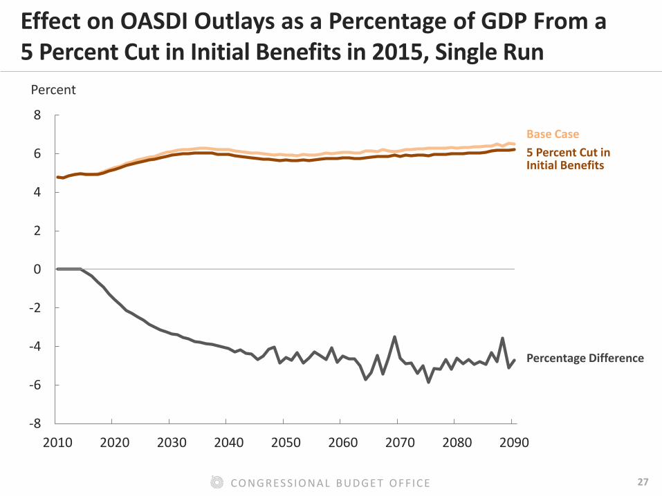
Example: A 5 Percent Cut in Initial OASDI Benefits, Single Run

■ The path of changes has a lot of noise even after the effect of the policy is fully phased in.

■ When the effect is fully phased in, annual changes could be 3.5 percent to 6 percent, depending on the year.

27 CO NGRES S IO NA L BUDGE T O F F IC E

Effect on OASDI Outlays as a Percentage of GDP From a 5 Percent Cut in Initial Benefits in 2015, Single Run

-8

-6

-4

-2

0

2

4

6

8

2010 2020 2030 2040 2050 2060 2070 2080 2090

Percent

Base Case

5 Percent Cut in Initial Benefits

Percentage Difference

28 CO NGRES S IO NA L BUDGE T O F F IC E

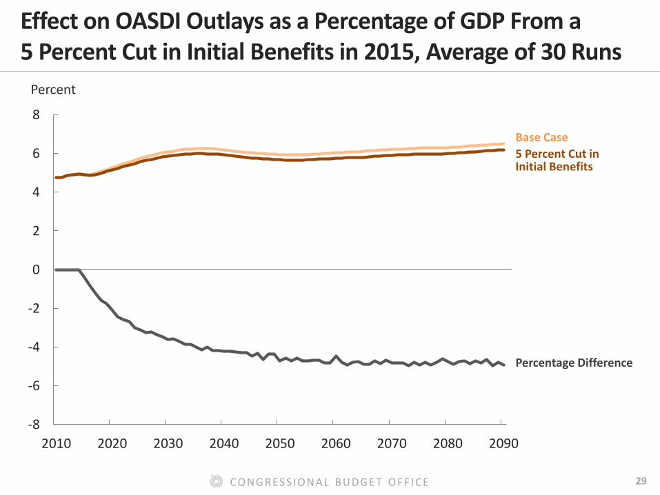
Example: A 5 Percent Cut in Initial OASDI Benefits, Average of 30 Runs

■ The paths of outlays as a percentage of GDP are smoother, and the path of changes is much smoother, varying only from about 4.7 percent to 4.9 percent once the effect is fully phased in.

■ Noise is a function of the number of runs; more could be used.

29 CO NGRES S IO NA L BUDGE T O F F IC E

Effect on OASDI Outlays as a Percentage of GDP From a 5 Percent Cut in Initial Benefits in 2015, Average of 30 Runs

-8

-6

-4

-2

0

2

4

6

8

2010 2020 2030 2040 2050 2060 2070 2080 2090

Percent

Base Case

5 Percent Cut in Initial Benefits

Percentage Difference

30 CO NGRES S IO NA L BUDGE T O F F IC E

Example: A 5 Percent Cut in Initial OASDI Benefits, Effects on the Actuarial Shortfall

■ Center of distributions improves the shortfall by 0.7 percentage points of taxable payroll (16 percent)

■ Estimate of improvement could be skewed if single runs are used and outcomes are outliers

– “Outside” outliers would show an improvement of 0.9 percentage points (20 percent)

– “Inside” outliers would show an improvement of 0.4 percentage points (10 percent)

31 CO NGRES S IO NA L BUDGE T O F F IC E

Distribution of OASDI 75-Year Actuarial Shortfalls in the Base Case and With a 5 Percent Cut in Initial Benefits

0.00

0.05

0.10

0.15

0.20

0.25

3.5 3.6 3.7 3.8 3.9 4.0 4.1 4.2 4.3 4.4 4.5

Percentage of Taxable Payroll

Frequency

With a 5 Percent Cut in Initial Benefits

(30 Runs)

Base Case (100 runs)

32 CO NGRES S IO NA L BUDGE T O F F IC E

Conclusion

■ Monte Carlo variation exists in all microsimulations.

■ Minute changes to policy or the model create propagating changes; these changes are essentially Monte Carlo variation.

■ Both triggers of variation can cloud outcomes.

■ Techniques exist to minimize the negative effects.

■ Knowing the distribution of Monte Carlo variation for outcomes of interest helps determine the appropriate technique.