1 Investigating Rationality in Wage-Setting Sonia R. Bhalotra University of Cambridge & University of Bristol, UK Abstract This paper investigates the efficiency wage hypothesis and derives a tractable expression for the profit loss incurred by deviations from the efficiency wage. The extent of the wage deviation can be inferred from production function parameters. The resulting profit loss is shown to depend upon the curvature of the effort function and the employment and wage elasticities of output. If the profit loss is small then near rationality may be claimed even if the hypothesis of rationality is statistically rejected. An application to Indian manufacturing is presented, which suggests that rationality cannot be rejected and that the profit function is remarkably flat around the optimum. This is consistent with positive effort returns to increasing the wage beyond its efficient level. Keywords: efficiency wages, near-rationality, panel data, India. JEL classification: J41, C23, O15 Contact Address: Department of Applied Economics University of Cambridge Sidgwick Avenue, Cambridge CB3 9DE, UK Email: [email protected]Telephone: +44 1223 335255
Transcript
1
Investigating Rationality in Wage-Setting
Sonia R. Bhalotra
University of Cambridge & University of Bristol, UK
Abstract
This paper investigates the efficiency wage hypothesis and derives a tractable expression for the
profit loss incurred by deviations from the efficiency wage. The extent of the wage deviation can
be inferred from production function parameters. The resulting profit loss is shown to depend upon
the curvature of the effort function and the employment and wage elasticities of output. If the
profit loss is small then near rationality may be claimed even if the hypothesis of rationality is
statistically rejected. An application to Indian manufacturing is presented, which suggests that
rationality cannot be rejected and that the profit function is remarkably flat around the optimum.
This is consistent with positive effort returns to increasing the wage beyond its efficient level.
Keywords: efficiency wages, near-rationality, panel data, India.
This paper is concerned with testing rationality and the weaker condition of near-rationality
in an environment in which worker effort is a function of the wage. Deviations of the wage from its
efficient level are regarded as consistent with near-rationality if the profit losses incurred as a result
are small. There is no rigorous definition of “small” just as there is no particular guide to choosing a
statistical significance level. However, one may think of small profit losses as comparable to
information or transactions costs that firms may have to incur to adjust to the efficient point.
Alternatively, the firm may pay more than the efficiency wage in order to avoid the costs that a
dissatisfied union may impose. Rent-sharing may be encouraged in efficiency wage environments
since increasing the wage beyond its optimal level yields positive, if diminishing, effort returns.
When effort depends on the wage, then firms can increase output in the short run either by
increasing employment or by increasing the wage. The wage bill is symmetric in these alternatives.
Therefore, at the optimal or efficiency wage, the wage elasticity of output equals the employment
elasticity of output. If the data do not support this condition, we conclude that firms are not exercising
rationality in wage setting2. It is then worth investigating whether the data satisfy the weaker
condition of near rationality. On the other hand, if rationality cannot be statistically rejected, it is not
strictly necessary to investigate near rationality. However, it may nevertheless be useful as a means of
confirming the “statistical metric” with an “economic metric”. The difference in the point estimates
of the output elasticities of the wage and employment can be cast in terms of the implied deviation of
the wage from its optimal level. Profit loss can then be calculated as a function of the wage deviation,
1 This paper has benefited greatly from the comments of David Demery, Nigel Duck, Ian Jewitt, JohnMuellbauer and, not least, Steve Nickell.
3
the employment elasticity of output, and the curvature of the effort function. It is interesting to find
out whether the profit loss is big or small, be it of second-order.
These questions are investigated using a panel of data for Indian manufacturing. The Indian
labour market does not appear to be competitive (see Section 5), and investigation of the efficiency
wage hypothesis seems the natural route to investigating profit maximising behaviour. The natural
alternative hypothesis is that wages paid in the primary sector exceed the optimal wage on account of
the influence of unions and government. We obtain GMM estimates of a production function that
includes wage-dependent effort. Careful attention is paid to potential biases arising from
heterogeneity, endogeneity and measurement error, and the results are subjected to various robustness
checks. The literature concerned with industrialised economies proposes that efficiency wages are
paid to recruit, retain and motivate workers, and effort is usually taken to be a function of the relative
wage. In a low-income country, an alternative reason for firms to offer wages in excess of market-
clearing is that this might enable greater effort for physical reasons. In this case, effort is a function of
the consumption wage. The model in this paper is specified so as to permit both the recruit-retain-
motivate and the enable possibilities.
Section 2 describes existing research on the subject, delineating the contributions of this
paper. Section 3 sets out the basic theory and the optimality condition, while Section 4 derives
conditions that obtain in the neighbourhood of the optimum. Section 5 develops the Indian context.
Section 6 develops an empirical specification and describes the data and issues arising in estimation.
The estimates are discussed in Section 7. In Section 8, profit losses arising from deviations from the
efficiency wage are calibrated for alternative values of the parameter describing the curvature of the
effort-wage function. Section 9 concludes.
2 Rationality is used in this paper to refer to profit maximising behaviour given a technology in whicheffort is wage dependent.
4
2. Existing Work And Contributions
Although the efficiency wage hypothesis has a long history (see Dunlop, 1988), empirical
investigations of it are still rather scarce. A fairly recent crop of studies documents persistent inter-
industry wage differentials that are only marginally narrowed once controls for worker and job traits
are introduced (e.g., Dickens and Katz 1987, Krueger and Summers, 1987). While such evidence is
consistent with the efficiency wage hypothesis it does not, on its own, persuade the sceptic that
efficiency wages are paid since competition and rent-sharing cannot be ruled out as alternative
explanations. Other studies have sought to establish a positive correlation of high wages with
measures of performance such as quits, absenteeism, or job satisfaction (see Katz 1986, Katz and
Summers 1989). While these have the advantage of possibly discriminating between alternative
efficiency wage models, they depend upon the availability of data on quits, satisfaction, etc. This
paper takes the more direct approach of testing the optimality condition that derives from profit-
maximising behaviour when the production function includes wage-dependent effort. Wadhwani and
Wall (1991) and Levine (1992) take a similar approach, using company data for the UK and the US
respectively. There are differences in methodology between the three studies. This paper augments a
small body of evidence based on direct testing, and an even smaller body of evidence providing
results for a developing country.
The paper does not stop with a statistical test of rationality but investigates the latitude
available to near-rational behaviour in terms of deviating from the efficiency wage. This is expected
to deliver a better handle on the degree to which any data sample supports the optimality condition
than can be had from statistical testing alone. The idea of near rationality is discussed by Akerlof and
Yellen (1985a, 1985b). Akerlof (1979) investigates this, showing that considerable deviations from
optimal money holdings are associated with trivial costs. In a similar spirit, Cochrane (1989) shows
that deviations from the rule for intertemporal allocation of consumption implied by the permanent
income hypothesis result in very small losses in utility. There does not appear to have been any
5
attempt to investigate near rationality in an efficiency wage setting. This paper sets out a structure for
doing this and provides some empirical results for a sample of Indian industries.
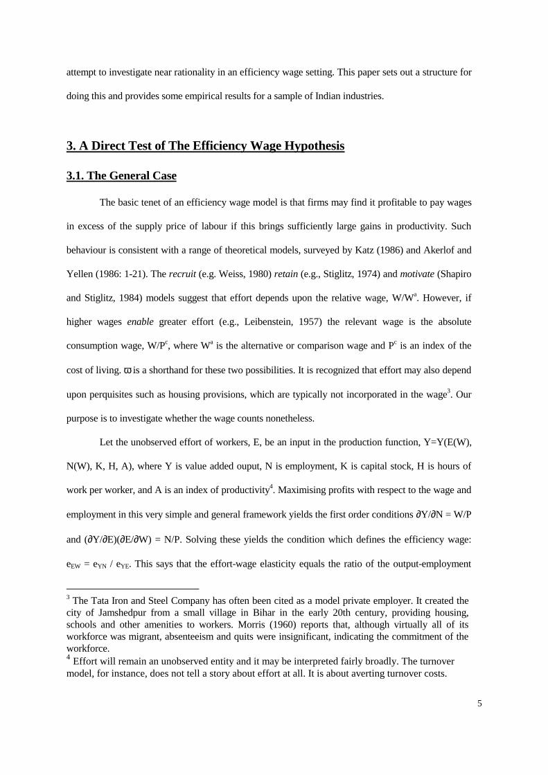
3. A Direct Test of The Efficiency Wage Hypothesis
3.1. The General Case
The basic tenet of an efficiency wage model is that firms may find it profitable to pay wages
in excess of the supply price of labour if this brings sufficiently large gains in productivity. Such
behaviour is consistent with a range of theoretical models, surveyed by Katz (1986) and Akerlof and
Yellen (1986: 1-21). The recruit (e.g. Weiss, 1980) retain (e.g., Stiglitz, 1974) and motivate (Shapiro
and Stiglitz, 1984) models suggest that effort depends upon the relative wage, W/Wa. However, if
higher wages enable greater effort (e.g., Leibenstein, 1957) the relevant wage is the absolute
consumption wage, W/Pc, where Wa is the alternative or comparison wage and Pc is an index of the
cost of living. ω is a shorthand for these two possibilities. It is recognized that effort may also depend
upon perquisites such as housing provisions, which are typically not incorporated in the wage3. Our
purpose is to investigate whether the wage counts nonetheless.
Let the unobserved effort of workers, E, be an input in the production function, Y=Y(E(W),
N(W), K, H, A), where Y is value added ouput, N is employment, K is capital stock, H is hours of
work per worker, and A is an index of productivity4. Maximising profits with respect to the wage and
employment in this very simple and general framework yields the first order conditions ∂Y/∂N = W/P
and (∂Y/∂E)(∂E/∂W) = N/P. Solving these yields the condition which defines the efficiency wage:
eEW = eYN / eYE. This says that the effort-wage elasticity equals the ratio of the output-employment
3 The Tata Iron and Steel Company has often been cited as a model private employer. It created thecity of Jamshedpur from a small village in Bihar in the early 20th century, providing housing,schools and other amenities to workers. Morris (1960) reports that, although virtually all of itsworkforce was migrant, absenteeism and quits were insignificant, indicating the commitment of theworkforce.4 Effort will remain an unobserved entity and it may be interpreted fairly broadly. The turnovermodel, for instance, does not tell a story about effort at all. It is about averting turnover costs.
6
elasticity to the output-effort elasticity. Neither eEW nor eYE is observable but rearranging gives eYE
eEW = eYN, or
eYW = eYN (1)
The elasticities in (1) are estimable. If the elasticity of output with respect to the wage equals its
elasticity with respect to employment, then the firm is paying the efficiency wage. This wage pays for
itself. The intuition is straightforward. Since the wage bill is symmetric in W and N, the equilibrium
must have the property that the marginal increase in N is as productive as the marginal increase in W.
If wage bargaining coexists with efficiency wage considerations, we may expect that the agreed wage
exceeds the pure efficiency wage. In that case, eYW < eYN, or the wage does not quite pay for itself.
Notice that the Solow condition, eEW = 1, is a special case of eEW = eYN / eYE that arises if and only if
effort is specified as labour-augmenting (i.e., eYN = eYE).
3.2. A Theoretical Structure
It is useful to impose some structure on the effort and production functions for purposes of
the analysis in Section 4. Let the production function incorporating effort be
Y = A Kβ Hµ Nα[E(ω)]α ν (2)
where ν is an i.i.d. productivity shock that is assumed to be uncorrelated with changes in A, N, K and
H. Departing from the tendency to assume that hours is labour-augmenting (Abramovitz (1950),
Solow (1957)), we do not restrict µ to equal α. In fact, since additional hours are expected to increase
capital utilization while additional workers may be knocking elbows over the same capital stock, it is
expected that µ>α (consistent with Feldstein (1967) and Craine (1973)). On the other hand, effort is
specified as a perfect substitute for employment. While this does not affect the optimality condition,
it simplifies the ensuing profit loss calculations. Let
E = -θ + ωδ ; 0 < δ <1 (3)
However, like the rest of the literature, we think of the saving in turnover costs as similar to an
7
E'(ω)>0 and E''(ω)<0, or there are positive but decreasing returns to increasing the wage. Now to
avoid clutter, A, K and H are suppressed because they do not depend upon the wage5. The function
we work with is
Y = Nα [-θ + ωδ]α (4)
A negative intercept is specified in the effort function so as to rule out the possibility of non-negative
effort at a zero wage. If θ≤0, then the zero wage is the efficiency wage6.
If π = PY-WHN, then hourly profit is π/Η = (P/H)Y-WN. Henceforth, P will refer implicitly
to (P/H) and π to π/Η. This is unrestrictive since P and H are treated as constants. The first order
conditions for profit maximisation are
∂π/∂N = 0 ⇒ αY/N - W/P = 0 (5)
∂π/∂W = 0 ⇒ P∂Y/∂W- N = 0 (6)
Define
γ ≡ ∂lnY/∂lnW = W/Y (∂Y/∂W) (7)
Together (5), (6) and (7) imply the optimality condition,
γ = WN/PY = α (8)
increase in unobservable effort.5 While it is clear that A and K do not depend upon the wage, the suggested independence of H needsjustification. Recall that hours here refers to actual as opposed to official hours. We suspect thatvariation in actual hours is substantially driven by forces such as the unavailability of crucialimported inputs or the rationing of power supplies by the government (Bhalotra (1995) presents someevidence to this effect). These tend to be outside the control of the individual firm or industry.6 It is straightforward to demonstrate this. Without any loss of generality, let ω=(W/Pc). Now if θ=0,then π = [PNα ωαδ - PcωN] = [PNα(1-δ) (ωN)αδ - Pc(ωN)]. From this, it is clear that π can be madearbitrarily large by making N large while keeping ωN (costs) constant. In other words, the optimum isat N=∞, W=0. Now let θ>0. Then π = [PNα (θ + ωδ)α - PcωN] ≥ [PNαθα - PcωN] and, as before, it isclear that profits can be expanded infinitely by raising employment, keeping the wage close to zero.Also see Akerlof (1982).
8
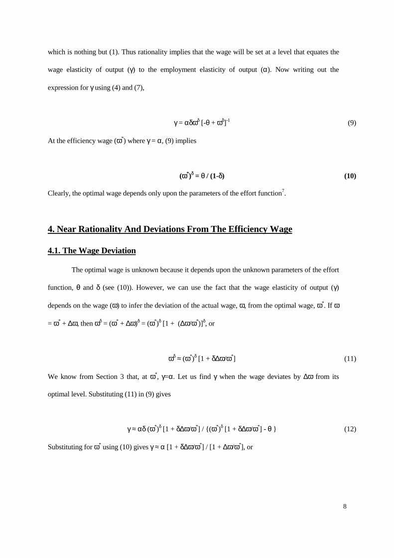
which is nothing but (1). Thus rationality implies that the wage will be set at a level that equates the
wage elasticity of output (γ) to the employment elasticity of output (α). Now writing out the
expression for γ using (4) and (7),
γ = αδωδ [-θ + ωδ]-1 (9)
At the efficiency wage (ω*) where γ = α, (9) implies
(ω*)δ = θ / (1-δ) (10)
Clearly, the optimal wage depends only upon the parameters of the effort function7.
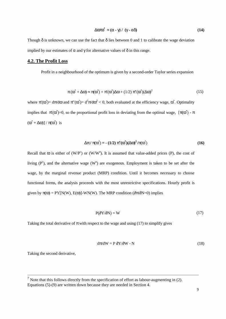
4. Near Rationality And Deviations From The Efficiency Wage
4.1. The Wage Deviation
The optimal wage is unknown because it depends upon the unknown parameters of the effort
function, θ and δ (see (10)). However, we can use the fact that the wage elasticity of output (γ)
depends on the wage (ω) to infer the deviation of the actual wage, ω, from the optimal wage, ω*. If ω
= ω* + ∆ω, then ωδ = (ω* + ∆ω)δ = (ω*)δ [1 + (∆ω/ω*)]δ, or
ωδ ≈ (ω*)δ [1 + δ∆ω/ω*] (11)
We know from Section 3 that, at ω*, γ=α. Let us find γ when the wage deviates by ∆ω from its
where π′(ω*)= dπ/dω and π′′(ω*)= d2π/dω2 < 0, both evaluated at the efficiency wage, ω*. Optimality
implies that π′(ω*)=0, so the proportional profit loss in deviating from the optimal wage, [π(ω*) - π
(ω* + ∆ω)] / π(ω*) is
∆π / π(ω*) = - (1/2) π″(ω*)(∆ω)2 /π(ω*) (16)
Recall that ω is either of (W/Pc) or (W/Wa). It is assumed that value-added prices (P), the cost of
living (Pc), and the alternative wage (Wa) are exogenous. Employment is taken to be set after the
wage, by the marginal revenue product (MRP) condition. Until it becomes necessary to choose
functional forms, the analysis proceeds with the most unrestrictive specifications. Hourly profit is
given by π(ω) = PY[N(W), E(ω)]-WN(W). The MRP condition (∂π/∂N=0) implies
P(∂Y/∂N) = W (17)
Taking the total derivative of π with respect to the wage and using (17) to simplify gives
dπ/dW = P ∂Y/∂W - N (18)
Taking the second derivative,
7 Note that this follows directly from the specification of effort as labour-augmenting in (2).Equations (5)-(9) are written down because they are needed in Section 4.
where we have used the fact (see (8)) that π(W*) = PY*-W*N* = PY*(1-α). With (14), the wage-
deviation term in (30) can be eliminated if one wants an expression for profit loss in terms of α, γ and
δ instead of in terms of α, δ and a wage deviation.
8 Recall that a given percentage increase in employment has the same effect on costs (the wagebill) asthe same percentage increase in the wage so that, at the efficiency wage, the output produced bymarginal changes in employment and the wage is equal (Section 3).
12
5. The Indian Context
The efficiency wage hypothesis predicts involuntary unemployment, labour market
segmentation, and inter-industry wage-differentials, all of which are strikingly evident in the Indian
economy. In 1987/88, 6% of males and 8.5% of females in urban India were unemployed for the most
part of the preceding year (Sarvekshana, 1990). In the absence of state-provided unemployment
benefits, one might expect that reservation wages are low and unemployment amongst the poor is
involuntary. The primary-secondary sector dualism highlighted by Doeringer and Piore (1971) is
particularly striking in low-income countries. For instance, primary sector wages in India are, on
average, more than twice secondary sector wages (Rs. 42 vs. Rs. 17 per day for urban males:
Sarvekshana (1990)). Within the primary sector, apparently permanent inter-industry wage
differentials suggest that, consistent with the efficiency wage model, technological factors play a role
in wage determination. For instance, in registered manufacturing (or equivalently, the factory sector),
nominal earnings in Transport Equipment were four and a half times those in Tobacco & Beverages
during 1979-1987. This might reflect, amongst other things, a tendency for output in the former
industry to be more sensitive to effort than in the latter industry. The industry wage differences
display no tendency to convergence. The weighted standard deviation of the log of industry wages is
46%, a far greater spread than observed in other countries, for example, the US (24%), the UK
(14%), Sweden (8%) and Mexico (15%) (see Krueger and Summers, 1987)). India is a big country,
and the substantial variation in human capital across its states might be thought to explain this
dispersion to a large extent. However, the within-state dispersion of industry wages is also very large,
ranging from 30% in Rajasthan to 83% in Kerala. The year-by-year rank correlations of the industry
wage structure are about 0.95 on average. Adjusting for location and for regional price variation does
not make wage dispersion much smaller and the ranks hardly change at all (see Bhalotra, 1995).
Productivity and other industry-specific variables are significant in factory wage determination (e.g.,
Bhalotra, 1995). Moreover, an analysis of regional unemployment rates in India indicates support for
a queueing model (Bhalotra, 1996a), which suggests that the observed wage differentials denote a
13
utility differential. They do not appear to be the compensating differentials that fall neatly within the
scope of perfectly competitive models of the labour market.
Investigation of the efficiency wage hypothesis in the Indian context is topical. There is a
widespread view that the Indian factory worker earns “too much”, both with regard to the pay
differential between factory and non-factory sector workers, and with regard to the prospects for
factory employment growth (e.g., Lucas 1988, World Bank 1989). This view gathered momentum in
the 1980s, when product wages in factories accelerated and factory employment declined. Its
adherents demand policy reforms that curb union power and revoke job security legislation. Indeed,
these demands are currently central to the controversy over India's new economic policies which, so
far, have concentrated on product market deregulation. Unions and job protection are thought to
nurture wage push and, thereby, to conflict with the objective of encouraging private enterprise9. It
has not been recognized, in this context, that private manufacturers might have volunteered wage
increases and that this is consistent with profit maximization on their part. Nor has it been appreciated
that wage-induced effort might have contributed to the remarkable increase in the rate of total factor
productivity growth in the 1980s. Deshpande (1992, p.91) appears to be an exception. In a comment
on analyses of the productivity turnaround in India, he admits the possibility that rising consumption
wages improved nutrition and morale. But, he says, “these logical possibilities are rarely entertained
for want of attempts at empirical verification”.
9 Note that traditional models of the development process have also tended to assume that wagedetermination in the registered sector is `institutional' (eg., Lewis 1954, Harris and Todaro, 1970).
14
6. An Empirical Specification
6.1. Data and Variables
For reasonably small changes in the wage, the production function (2) can be approximated
by a loglinear equation in which α and γ are estimable parameters (see Appendix 1).
The data used are a panel of 18 two-digit industries disaggregated by their location across the
15 major Indian states and observed annually during 1979-87 (see the Data Appendix). Availability
of the regional dimension is an advantage as it permits the comparison wage and the cost of living to
be defined at the state level. It also permits controls for industry-region fixed effects on productivity.
Regional variance in productivity can be especially large in developing countries, for example, on
account of their limited infrastructural development and relatively slow diffusion of skills. Firm-level
data were not available for Indian manufacturing. However, if we are willing to assume constant
returns to scale and common capital-labour ratios across firms then it is straightforward to
demonstrate that the aggregation implicit in specifying an industry-level production function is
valid10. Using subscripts i, s and t for industry, state and year, the estimated equation is
where τt are time dummies denoting productivity growth common to the industry-state units
including, for example, the effects of changes in the competitiveness of the manufacturing sector. ais
are unobserved time-invariant efficiency effects and εist is stochastic.
The book value of capital stock (Kist) is adjusted to get gross stock at replacement cost.
Employment (Nist) refers to production workers and supervisory staff. The ratio of production to non-
production workers is 2:1. In the absence of skill-disaggregated data, this ratio was included in the
production function as a proxy for skill. It emerged with a completely insignificant coefficient. So as
to streamline the discussion, it is not discussed any further. Value added (Yist) is available in nominal
15
terms and is deflated by the wholesale price index for industry output (Pit). Single-deflation in this
manner may bias the estimated parameters if the ratio of input to output prices experienced
considerable industry-time variation in the period of the study. However, Bhalotra (1996b)
investigates controls for input prices and finds no change in the estimates. Nevertheless, as a check on
the robustness of our results to the omission of any industry-time varying variables including material
prices and labour quality, we shall report estimates of a production function that includes industry-
time dummies (τit) (Section 7.3). Actual hours worked per worker (Hist) is a utilization variable that
averages overtime and “undertime” across workers and over time. Thus overtime or multiple shifts
per worker may result in actual hours exceeding official hours, whereas input shortages may result in
actual hours falling below official hours. Of course actual time worked is precisely what is desired in
a production function11.
The wage (ωist) refers, in different specifications, to the consumption wage and the relative
wage. In both cases, the numerator is earnings per hour of actual work. Deflating this by a regional
cost of living index (Pcst) gives the consumption wage. Pcst is defined uniquely for the category of
industrial workers for every Indian state. To obtain a relative wage, we divide by Wst, the state
average of the factory wage. If the reference group or the relevant alternatives of factory workers lie
outside the factory sector, incomes in the rural and urban informal sectors might better represent the
alternative wage, Wa. In the absence of time-variant data on these variables, it is hoped that they will
be adequately proxied by Wst. This is defensible if the sectoral wage structure in a state is fairly rigid.
Alternatively, the time dummies (τt) and fixed effects (ais) in the model will together control for state-
specific variables (xst) to a first-order approximation, xst = as + tt + εst. If the approximation is good, εst
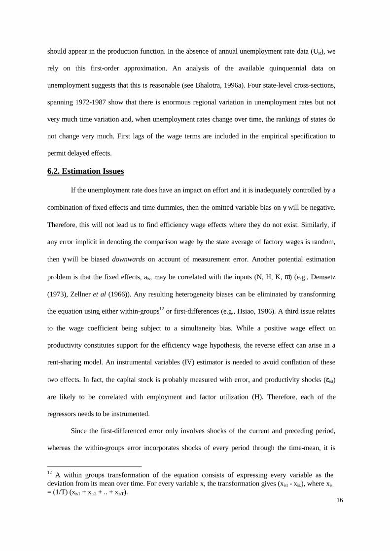
is random. If effort is stimulated not only by the wage but also by unemployment, then unemployment
10 See Bhalotra (1996b), which also investigates the pooling restrictions implicit in specifyingcommon slopes in the production function. It appears that pooling cannot be rejected though it mustbe said that relatively large standard errors on the GMM estimates create a bias towards this result.11 Muellbauer (1984) argues that finding an appropriate measure of utilization dominates the otherclassical problems arising in production function estimation, namely of aggregation andidentification. He proposes a variable that controls for actual hours and demonstrates that it makes asignificant contribution in the production function for British manufacturing.
16
should appear in the production function. In the absence of annual unemployment rate data (Ust), we
rely on this first-order approximation. An analysis of the available quinquennial data on
unemployment suggests that this is reasonable (see Bhalotra, 1996a). Four state-level cross-sections,
spanning 1972-1987 show that there is enormous regional variation in unemployment rates but not
very much time variation and, when unemployment rates change over time, the rankings of states do
not change very much. First lags of the wage terms are included in the empirical specification to
permit delayed effects.
6.2. Estimation Issues
If the unemployment rate does have an impact on effort and it is inadequately controlled by a
combination of fixed effects and time dummies, then the omitted variable bias on γ will be negative.
Therefore, this will not lead us to find efficiency wage effects where they do not exist. Similarly, if
any error implicit in denoting the comparison wage by the state average of factory wages is random,
then γ will be biased downwards on account of measurement error. Another potential estimation
problem is that the fixed effects, ais, may be correlated with the inputs (N, H, K, ω) (e.g., Demsetz
(1973), Zellner et al (1966)). Any resulting heterogeneity biases can be eliminated by transforming
the equation using either within-groups12 or first-differences (e.g., Hsiao, 1986). A third issue relates
to the wage coefficient being subject to a simultaneity bias. While a positive wage effect on
productivity constitutes support for the efficiency wage hypothesis, the reverse effect can arise in a
rent-sharing model. An instrumental variables (IV) estimator is needed to avoid conflation of these
two effects. In fact, the capital stock is probably measured with error, and productivity shocks (εist)
are likely to be correlated with employment and factor utilization (H). Therefore, each of the
regressors needs to be instrumented.
Since the first-differenced error only involves shocks of the current and preceding period,
whereas the within-groups error incorporates shocks of every period through the time-mean, it is
12 A within groups transformation of the equation consists of expressing every variable as thedeviation from its mean over time. For every variable x, the transformation gives (xist - xis.), where xis.
= (1/T) (xis1 + xis2 + .. + xisT).
17
easier to find instruments for a first-difference estimator, which is therefore preferred. Finally, there
is the question of consistency, given that the panel has a short time series. For these reasons, the
generalized method of moments (GMM) estimator proposed by Arellano and Bond (1991) is used.
This performs instrumental variables estimation on a first-differenced equation and produces
consistent estimates even on short panels. The instruments are the second and more remote lags of the
endogenous variables, which are valid under the assumption that the levels error is serially
uncorrelated, which is subject to testing. If the levels error is MA(1), then instruments dated t-2 are
invalid but instruments dated t-3, t-4, and earlier, are still valid. Simulations conducted by Arellano
and Bond indicate that use of remote lags, or additional moment restrictions, brings significant
efficiency gains. Two tests of instrument validity are provided with the GMM estimates. Serial
correlation(2) is a test for the absence of second-order serial correlation in the differenced residuals.
The test statistic is distributed as standard normal under the null of no serial correlation. Sargan is a
test for overidentifying restrictions. This is asymptotically distributed as chi-squared under the null of
instrument validity, with as many degrees of freedom as overidentifying restrictions.
7. Results: Do Indian Factories Pay Efficiency Wages?
7.1. Alternative Estimators
Table 1 explores alternative estimators of a production function that incorporates the relative
wage13. Since production function estimation is an important but difficult problem, the alternative
estimates are considered in some detail. Time dummies (θt) are included in every specification and
Wald tests (χ2k) show them to be jointly significant (k is the number of estimated coefficients). All
reported standard errors are heteroskedasticity-consistent. The first and second lags of the wage were
not significant and so they were not retained. WG in column 2 differs from OLS-levels in column 1 in
13 Since the specifications in Table 1 are only exploratory, only the final specifications are shown forthe consumer wage model, and these are in Table 2. Corresponding estimates of production functionswithout any wage term are presented in Bhalotra (1996b), where the alternative estimators arediscussed in more detail.
18
controlling for fixed efficiency effects at the industry-state level (ais). Comparison across these
columns demonstrates that the levels-OLS estimate of every parameter carries a substantial
heterogeneity bias. The within groups (WG, column 2) and first-difference (FD, column 3) estimates
are fairly similar, the slightly smaller estimates of β and µ in the latter case being consistent with
measurement error in K and H and with the resulting bias being larger under FD than under the WG
transformation (e.g., Griliches and Hausman, 1986). Griliches and Hausman (1986) show how the
WG and FD estimates can be combined to provide consistent estimates in the presence of
measurement error. Let x=x* + u, where x is the observed value of x*, u is measurement error, T is the
The corrected estimates are shown in column 4. However, if the WG and FD estimates are subject to
endogeneity bias in addition to measurement error bias, then this approach will not recover the true
coefficients. Therefore an instrumental variables estimator is used. Column 5 presents GMM
estimates which rely on the second to the fourth lags of lnNist, lnKist, lnHist, (lnWist - lnWst) and lnPcst
as instruments. Since there is no evidence of second-order serial correlation in the differenced
residuals, these instruments are not invalid (also see Sargan statistics in Table 1). The results suggest
that productivity shocks are positively correlated with employment and negatively correlated with
capital, hours and the wage. Note that the wage coefficient behaves rather similarly to the hours
coefficient as it responds to corrections for different sorts of bias. Column 6 presents the two-step
estimates which use the residuals from the one-step estimates in column 5 to create the asymptotically
optimal weighting matrix in the presence of heteroskedasticity. While the two-step estimates are
asymptotically more efficient, they appear to have spuriously small standard errors in small samples
(Arellano and Bond, 1991). Indeed, standard errors on our two-step coefficients are about a third of
those on the one-step coefficients. Therefore the estimates in column 5 are preferred. In view of the
discussion in Section 6.2, we are only concerned with its size in the GMM models.
19
7.2. Investigating Restrictions
Table 2 reports one-step GMM estimates for the relative wage (lnWist-lnWst) and the
consumer wage (lnWist-lnPcst) models. Wald tests of restrictions are reported in Notes to the Table.
Column 1 in each panel shows the unrestricted estimates corresponding to column 5 in Table 1. In the
other columns, constant returns to scale are imposed since this is data consistent and is a clean way of
dealing with measurement error in K, the effects of which are not guaranteed to be taken care of using
lags of K as instruments. Columns 2 impose the additional restriction, common in the literature, that
the coefficient on hours equals that on employment. The relevant α is then the coefficient on total
person-hours. An advantage of this specification is that a test of the efficiency wage condition (γ=α)
is robust to the problem that firms varying employment incur adjustment costs. While this provides a
useful check on the model, we prefer the estimates in columns 3 where the coefficient on hours is
restricted to equal unity. The Wald tests of the alternative restrictions on hours greatly favour the µ=1
restriction. Scaling output by hours is also theoretically appealing since, when a worker puts in an
additional hour, capital services, fuel and other inputs will typically be utilised for the additional
hour. Both restrictions buy us greater efficiency which is fairly important with GMM estimates.
7.3. Testing the Efficiency Wage Hypothesis
Across a range of estimators and, irrespective of restrictions, the wage has a significantly
positive effect on productivity. In every GMM model in Table 2, the efficiency wage condition,
α=γ, cannot be rejected (t-statistics in Table 2). There is thus fairly compelling evidence that
efficiency wages are paid and that these pay for themselves. For further discussion, we shall take
columns 3 as the preferred model.
With regard to the significance of the relative wage, it is worth recalling that the evidence
presented here pertains to the factory sector, which is the primary or `formal' manufacturing sector. It
includes all of the relatively big firms, in which moral hazard and other information problems are
likely to be relatively severe. In addition, these tend to be relatively capital and technology intensive
20
firms, the output of which may be more sensitive to effort variations than is the case in very small
firms. It is the tendency for such enterprises to select themselves into the primary or formal sector
labour market that gives rise to formal-informal sector wage dualism (Akerlof, 1982). Significance of
the consumption wage supports the “enable” hypothesis. Although the average production worker in
the Indian factory has crossed the subsistence level of income, food still claims almost two-thirds of
the family budget (Chatterji, 1989). Increments to their wages might therefore be associated with
visible increases in well-being. For example, the worker might consume higher quality foods, or
avoid a long commute to work14. Bhalotra (1997) discusses the relevance of the alternative efficiency
wage models to the Indian setting.
7.3. Robustness
We have already investigated robustness of the positive wage effect on productivity to
alternative estimators and alternative data-consistent restrictions on the production function
parameters. The (k-n)2 term implied by both a Taylor series approximation to a CES technology, and
the Translog function under CRS is insignificant on this data sample, as are lags of the regressors (see
Bhalotra, 1996b). Therefore, in this sample, the Cobb-Douglas model provides a reasonable
approximation to the actual technology. By virtue of controlling for actual hours, the specification
distinguishes the output effects of observed worker effort (or utilization) from those of unobserved
effort. Having time dummies rather than a trend affords a flexible characterization of aggregate
productivity growth. As mentioned earlier, the GMM estimates are expected to be clear of biases
arising from unobserved heterogeneity, endogeneity, and measurement error. Taking care of
endogeneity of the wage is particularly important since it eliminates any concern with the efficiency
wage effect being conflated with a rent-sharing effect working in the opposite direction15. Note also
14 Myers (1958:49-50) cites company officials in Indian industry in 1954 as saying that the Indianworker would be as efficient as any, were it not for poor nutrition and bad living conditions at homeand unsympathetic supervisors at work. Living standards of factory workers have improved since1954. Whether the real consumption wage had any impact on productivity in the 1980s meritsinvestigation.15 In the long run, industry productivity growth may be expected to be passed on to the widerpopulation as lower product prices. In developed countries, this typically implies a rise in the
21
that our measure of output is real value added. In studies that use the nominal output of firms, a
positive wage-productivity correlation can arise from rent sharing whence an increase in prices and
wages following an increase in market share (e.g., Levine, 1992).
However, interpretation of a positive wage coefficient in the production function as an
efficiency wage effect is still subject to the criticism that the positive wage effect arises from
inadequate controls for skill shifts. If there are industry-specific changes in skill-composition over
time, then industries that are raising skill levels will probably exhibit increases in wages and
productivity even in the absence of an efficiency wage mechanism. So as to control comprehensively
for skill shifts, the production function is re-estimated with a full set of interaction terms between
industry and time dummies (λiτ t). The 136 additional terms are included on the strength of the
regional variation in the data. Relative to columns 3 of Table 2, the employment coefficient increases
by one standard error and the relative wage coefficient falls by less than a standard error. In the
alternative specification with the consumer wage, both the employment and the wage coefficients
increase, but both changes are insignificant. Since GMM estimates of the model with industry-time
dummies are not very precisely determined, the model was also estimated by within groups. The
changes in the wage and employment coefficients were even smaller. Therefore it appears unlikely
that the wage effect is proxying a skill effect.
There is no reason for either of the output-effort or the effort-wage functions to be common
across sectors but suitable disaggregate data are unavailable. To investigate this matter, we estimate a
model with industry-specific wage coefficients. Since 17 additional terms need to be instrumened,
GMM is very inefficient. Within-groups estimates produce a significant positive wage effect in half
of the eighteen industries in the sample16. It would be interesting to explain the industry differences in
consumer wage and so it could account for reverse causality in the absence of insider wage push.However, in agrarian economies like India, the consumer price index is largely determined byagricultural prices, making this connection more tenuous. Therefore, a productivity impact on wagesrelies upon rent-sharing or efficiency wage models.16 In the specification with the relative wage, these are Chemicals, Basic metals, Machinery, Non-metallic minerals, Petroleum and rubber, Paper and publishing, Tobacco and beverages, Textile
22
terms, for example, of differences in the sensitivity of output to variations in effort, firm size and
monitoring costs, location and regional unemployment, or union power. This is beyond the scope of
the present study but provides an interesting avenue for research with more disaggregate data.
So far, worker effort has been permitted to depend either on the relative wage or on the
consumer wage. A third possibility, the adaptation hypothesis, is that effort depends on current
income relative to past income (see Goodman (1974), Akerlof (1982)). This is proxied here by ∆(wist-
pcst), and it turns out to be insignificant. Finally, the production function is estimated with the nominal
wage (wist), the alternative wage (wst) and the consumer price index (pstc) appearing as three
independent terms. The point of this exercise is to determine the “natural” denominator for the
nominal wage. The nominal wage acquires a significant coefficient (t=2.1) of 0.55. The coefficient on
wst is exactly equal and opposite in sign but it is insignificant. The coefficient on the index, pstc, is
significant but it is much larger than on wist. These results do not have an unambiguous interpretation.
In conclusion, there is robust evidence that efficiency wages are paid and that these pay for
themselves. In different specifications, the data support both the relative wage and the consumer
wage. The profit-maximising condition, that α and γ are identical, cannot be statistically rejected.
8. Investigation of Near Rationality in Wage-Setting
Given that we cannot reject rationality, it is not strictly necessary to investigate near
rationality. The methods outlined may be more fruitfully applied to a data set that does reject the null
of rationality, and this section may be regarded as merely illustrative17. Since the point estimates of α
and γ are their most likely values, we use the fact that they are not identical to investigate the
curvature of the profit-wage function. Estimates used here are those in columns 3 of Table 2.
products, and “Other” (the residual industry). In the model with the consumer wage, a positiveefficiency effect is found in the same set of industries with the exception of Basic Metals. 17 Note that, if the two-step GMM estimates are favoured over the one-step estimates, then we canreject the null of equality of α and γ. However, since simulations suggest that the two-step GMMestimates are spuriously well-determined in small samples, and since this is the “conservative”strategy in this context, we have chosen to concentrate on the one-step estimates.
23
Illustrative Wage Deviations
Using (30), we compute the profit loss that would arise if the wage were to deviate by 1, 2, 5
and 10 per cent. The relative wage and the consumer wage models produce the same result since the
estimate of α is basically the same in the two models (Table 2). We do not know δ but do know that
0<δ<118. In fact, (14) implies the smaller range, 0<δ<(γ/α)19. The results in Table 3 and Figure 1
show that the profit function is very flat in the neighbourhood of the optimum. A deviation of 1% in
the wage results in no more than 0.002-0.006% of optimal profit being lost, and a 10% deviation in
the wage results in a profit loss in the region of 0.2-0.6%. These are trivial losses by most standards.
Notice that, for a given wage deviation, profit loss is decreasing in δ (see (30)). Intuitively, the larger
is δ, the greater is the effort-return to increasing the wage, and this mitigates the profit lost from
paying too much.
Wage Deviations Implied by the Data
Table 4 presents estimates of profit loss based on imputing rather than assuming the
percentage deviation of the wage from its optimum. The results are plotted in Figures 2a and 2b for
the relative wage and the consumer wage respectively. Equation (14) shows that ∆ω/ω* can be
inferred from the point estimates of α and γ if, as before, we assume different values for δ. In our
sample γ<α and it is evident from (14) that the wage deviation is positive or firms tend to pay more
than the efficiency wage. A natural scenario consistent with this is one in which unions are involved
in wage-setting. The wage deviation, and therefore the profit loss, is increasing in δ.
The results make two striking points. First, the α and γ estimated on our data, while
statistically insignificantly different from one another, are consistent with fairly large wage
deviations. Thus the wage deviates by at least 14% in the relative wage model and at least 23% in the
18 This is a strict inequality. If δ=0 then effort is not wage dependent. If δ=1 then the effort-wagerelation is linear but the more plausible situation is that there are decreasing effort returns toincreasing the wage or that the relation is concave to the origin.19 Suppose 1>δ>(γ/α). Simple rearrangement shows that this implies (-1)>(α-γ)/(γ-αδ)>(-∞) or, by(14), (-1)>∆ω/ω*>(-∞). The first inequality in this expression implies ω<0, which is absurd. Atδ=(γ/α), ∆ω/ω*=∞.
24
consumer wage model. Second, the profit losses are relatively small. To be more precise, one needs
to define what one considers as small. Like significance levels that, by convention, may lie between
1% and 10%, we might suppose that profit losses upto 10% are “small”20. Then our estimates for the
relative wage model are consistent with near rationality. However, the consumer wage model may
appear to violate near rationality if δ is larger than about 0.45. In this case we have the apparently
counter-intuitive result that, while rationality is not statistically rejected, near rationality, which relies
upon a different metric is. However, it is important to note that the exercise resulting in Table 4
involves the point estimates of α and γ which we know to be uncertain, and that the profit loss
calculations grow unreliable as the wage deviations grow larger since they rely upon a Taylor series
approximation of second-order21.
The following conclusions emerge. While the relevant elasticities (α=0.57, γ=0.50 when
ω=W/Wa or α=0.58, γ=0.47 when ω=W/Pc) are statistically not significantly different, their point
estimates imply that firms pay wages considerably higher than the efficient wage. This is useful
information with which to complement the standard statistical metric applied to testing the
predictions of economic models. Using UK company data, Wadhwani and Wall (1991) find α=0.65,
γ=0.39 and reject α=γ in favour of α<γ, which is consistent with union bargaining leading to wages
higher than the efficiency wage. In contrast, Levine (1992) finds, on U.S. company data, that α=0.27,
γ=0.46. The point estimates suggest that companies pay less than the efficiency wage but the data
cannot reject α=γ. Clearly, point estimates may diverge considerably more than they do on the Indian
data and yet be statistically consistent with the notion that firms are operating at an optimum.
20 This is just for expositional convenience. The reader can, of course, reinterpret Table 4 using anyalternative definition of “small”. As mentioned in the Introduction, a “small” loss may correspond insize to transactions or information costs or other costs (like those imposed by unions) associated withmoving to the optimum. Alternatively, they may be the sorts of losses that firms incur on account of“everyday” mistakes, or else losses that firms in competitive environments can survive.21 While this digresses from the main concern of the paper, it may be worth pointing out that a deviationin the wage from its optimal level implies a deviation in employment of the opposite sign. There hasbeen considerable concern in India regarding the slow growth in manufacturing employment (seeBhalotra, 1997).
25
The second result from our analysis is that the profit function is remarkably flat. It suggests
that, even though wage increases beyond the efficient wage do not pay for themselves, they stimulate
enough effort to mitigate the resulting profit loss. Thus in environments where effort is a positive
function of the wage, the profit-wage function will be flatter than otherwise. This makes some sense
of the fact that such large deviations are sustained. It might seem surprising that firms can sustain any
loss in profit loss without, for instance, incurring takeover (e.g. Cochrane, 1989). However, Indian
manufacturing in the 1980s was sufficiently protected from competition to make it possible for firms
to live with some degree of slack.
9. Conclusions
We cannot reject the hypothesis that efficiency wages are paid in Indian factories. The wage
effects are sizeable, the elasticities being about 0.5. In independent specifications, effort appears to be
stimulated by increases in the relative wage and in the absolute consumption wage. Significance of
the relative wage affords support for the “recruit-retain-motivate” class of models which is consistent
with informational deficiencies in the relatively large and capital intensive firms in the factory sector.
Significance of the consumption wage supports the “enable” hypothesis.
The profit function is remarkably flat in the neighbourhood of the optimum. A deviation of as
much as 10% from the efficiency wage results in a profit loss of, at most, 0.6%. The wage deviations
implied by our estimates of the production function parameters are a good bit larger than 10% but the
resulting profit loss is relatively small. This suggests two things. First, that, on average, Indian
factories do pay more than the efficiency wage, possibly on account of union intervention in wage-
setting. Second, this deviation from the optimum does not cost them very much, presumably because
positive productivity gains from increasing the wage beyond its efficient level compensate the profit
loss to some degree. Thus, near rational behaviour in a pure efficiency wage model is
indistinguishable from rational behaviour in a model in which efficiency wage considerations and
union wage bargaining coexist.
26
The popular view that factory wages incorporate substantial rents arising from imperfect
competition in product markets and extracted through union and government intervention is
undermined. While unions may have some influence on wage-setting, curbing union power is not
guaranteed to generate lower wages and higher employment in factories; and it would seem to be
technology rather than unionism that separates the informal from the formal manufacturing sector.
These results would, of course, be more convincing if they emerged from investigation of
firm-level data. This was not available. In general, firm data for developing countries are still scarce.
Were the necessary detail available, it would also be interesting to investigate efficiency wage setting
in public versus privately owned firms, in union versus non-union firms and in large versus small
firms. Further work is also desirable on the question of why efficiency wages are needed to elicit
effort. Important questions of the health and nutrition standards of workers at the one hand, and of job
security on the other are potentially tied in with an understanding of this: Do firms need to pay
efficiency wages because workers are unable to work hard unless they are paid uncompetitively high
wages, or because they all shirkers in the knowledge that their jobs are secure?
References
Abramowitz, M. (1950), Resources and output trends in the US since 1870, American Economic Review,Papers and Proceedings, 46: 5-23.
Aggarwal, A. (1991), Estimates of fixed capital stock in registered manufacturing sector in India, Indian Institute of Management Working Paper No. 937, Ahmedabad.
Akerlof, G. (1979), Irving Fisher on his head: The consequences of constant threshold-target monitoring of money holdings, Quarterly Journal of Economics, 93, May: 169-187.
Akerlof, G. (1982), Labor contracts as partial gift exchange, Quarterly Journal of Economics, 97(4): 543-69.
Akerlof, G. and J. Yellen (1985a), A near rational model of the business cycle with wage and price inertia, Quarterly Journal of Economics, 100, Supplement: 824-838.
Akerlof, G. and J. Yellen (1985b), Can small deviations from rationality make significant differences to economic equilibria?, American Economic Review, 75, September: 708-720.
Akerlof, G. and Yellen, J. (1986), Efficiency Wage Models of the Labour Market, Cambridge: Cambridge University Press.
Arellano, M. and Bond, S. (1991), Some tests of specification for panel data: Monte Carlo evidence and an application to employment equations, Review of Economic Studies, 58: 277-297.
Annual Survey of Industries (1979-87), Summary results for the factory sector, New Delhi: Central Statistical Organization.
27
Bhalotra, Sonia (1995), Wage determination, Chapter 3, Four Essays on the Urban Labour Market inIndia, DPhil. thesis, University of Oxford.
Bhalotra, Sonia (1996a), The spatial unemployment-wage relation revisited: An investigation of interstate urban unemployment rate differentials in India, Discussion paper 96/409, Department of Economics, University of Bristol.
Bhalotra, Sonia (1996b), Changes in utilisation and productivity in a deregulating economy, mimeograph, Department of Economics, University of Bristol.
Bhalotra, Sonia (1997), Near rationality and the efficiency wage, Manuscript, Department of Economics, University of Bristol.
Bhalotra, Sonia (1998), The puzzle of jobless growth in Indian manufacturing, forthcoming in the Oxford Bulletin of Economics and Statistics, February.
Chandok, H.L. and The Policy Group (1990), India Data Base: Annual Time Series data in 2 volumes, New Delhi: Living Media India Ltd.
Chatterji R. (1989), The Behaviour of Industrial Prices in India, New Delhi: Oxford University Press.Cochrane, J. (1989), The sensitivity of tests of the intertemporal allocation of consumption to near-
rational alternatives, American Economic Review, 79 (3), June: 319-337.Craine, R. (1973), On the service flow from labour, Review of Economic Studies, 40: 39-46.Demsetz, H. (1973), Industry structure, market rivalry and public policy, Journal of Law and
Economics, 16: 1-10.Deshpande, L.K. (1992), Institutional interventions in the labour market in Bombay's manufacturing
sector, in T.S. Papola and G. Rodgers (eds.), Labour Institutions and Economic Developmentin India, Research Series 97, International Institute for Labour Studies, ILO, Geneva.
Dickens, W. and Katz, L. (1987), Inter-industry wage differences and industry characteristics, inDoeringer, P. and M. Piore (1971), Internal Labour Markets and Manpower Analysis.
Dunlop, J. (1988), Labour markets and wage determination: Then and now, in B. Kaufman (ed.), How Labour Markets Work, Lexington, MA: DC Heath.
Feldstein, M. (1967), Specification of the labour input in the aggregate production function, Review of Economic Studies, 34: 375-86.
Goodman, P.S. (1974), An examination of referents used in the evaluation of pay, Organizational Behaviour and Human Performance, 12: 170-195.
Griliches, Z. and Hausman, G. (1986), Errors in variables in panel data, Journal of Econometrics, 31: 93-118.Harris, J. and Todaro, M. (1970), Migration, unemployment and development: A two-sector analysis,
American Economic Review, 60: 126-42.Hsiao, C. (1986), The Analysis of Panel Data, Cambridge: Cambridge University Press.Katz, L. (1986), Efficiency wage theories: A partial evaluation, in S.Fischer (ed.), NBER
Macroeconomics Annual, Cambridge, MA: MIT Press.Katz, L. and Summers, L. (1989), Industry rents: Evidence and implications, Brookings Papers on
Economic Activity: Microeconomics 1989, 209-275.Krueger, Alan and Summers, L. (1987), Reflections on the inter-industry wage structure, in K. Lang
and J. Leonard (eds.), Unemployment and the structure of labour markets, Oxford:Blackwell.Leibenstein, H. (1957), Economic Backwardness and Economic Growth, New York: John Wiley and
Son.Levine, D. (1992), Can wage increases pay for themselves? Tests with a production function,
Economic Journal, 102(414): 1102-1115.Lewis, W.A. (1954), Economic development with unlimited supplies of labour, Manchester School,
22: 139-191.
28
Lucas, R.E.B. (1988), India's industrial policy, in R.E.B. Lucas and G. Papanek (eds.), The Indian Economy: Recent Developments and Future Prospects, New Delhi: Oxford University Press.
Morris, Morris D. (1960), The labour market in India, in W.E. Moore and A.S. Feldman (eds.), Labour Commitment and Social Change in Developing Areas, New York: Social Science Research Council.
Muellbauer, J. (1984), Aggregate production functions and productivity measurement: A new look, CEPR Discussion Paper no. 34, London School of Economics.
Myers, C.A. (1958), Labour Problems in the Industrialization of India, Cambridge, Mass.: Harvard University Press.
Sarvekshana (1990), Journal of the National Sample Survey Organization, Central Statistical Organization, New Delhi: Ministry of Planning, September.
Shapiro, C. and Stiglitz, J. (1984), Equilibrium unemployment as a worker discipline device, American Economic Review, 74: 433-444.
Stiglitz, J. (1974), Alternative theories of wage determination and unemployment in LDCs: The labour turnover model, Quarterly Journal of Economics, 88: 194-227.
Sundaram, K. and Tendulkar, S. (1988), An approximation to the size structure of Indian manufacturing industry, in K.B. Suri (ed.), Small Scale Enterprises in Industrial Development: The Indian Experience, New Delhi: Sage Publications.
Wadhwani, S. and Wall, M. (1991), A direct test of the efficiency wage model, Oxford Economic Papers: 529-547.
Weiss, A. (1980), Job queues and layoffs in labour markets with flexible wages, Journal of Political Economy, 88: 526-538.
World Bank (1989), India: Poverty, Employment and Social Services, A World Bank Country Study, Chapter 4, Washington D.C.: The World Bank.
Zellner, A., Kmenta, J. and Dreze, J. (1966), Specification and estimation of Cobb-Douglas production models, Econometrica, 34: 784-95.
TABLES IN ATTACHED FILE
29
Appendix 1
Approximate Log Linearisation of the Production Function
A logarithmic transform of the production function in (4) is
y = αlnN + αln [-θ + ωδ] (1)
Since (1) is nonlinear, the following approximation is used. Let ω = ω0 + ∆ω, where ω0 is any wage
around which there is a small deviation, ∆ω, in the sample. Substituting for ω in (1) gives, to first-
Since αln[-θ + (ω0)δ] is a constant, and ln (1+z) ≈ z for small z, this implies
y = constant + αlnN + αδ(ω0)δ-1(∆ω)[-θ + (ω0)δ]-1 (4)
But αδ(ω0)δ[-θ + ωδ]-1 = γ (see (9)). Substituting in (4),
y = constant + αlnN + γ(∆ω/ω0) (5)
Using z ≈ ln(1+z) where z=(∆ω/ω0) and ω = ω0+ ∆ω, (5) implies y=constant + αlnN + γ log (ω/ω0).
Since γlog ω0 goes into the constant,
y = constant + αlnN + γ log ω (6)
This establishes that, for reasonably small changes in the wage, the production function can be
approximated by a loglinear equation in which α and γ are estimable parameters.
30
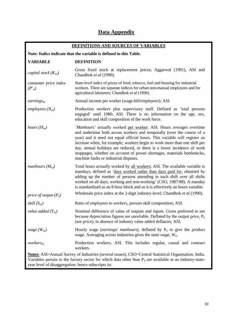
Data Appendix
DEFINITIONS AND SOURCES OF VARIABLES
Note: Italics indicate that the variable is defined in this Table.
VARIABLE DEFINITION
capital stock (Kist)Gross fixed stock at replacement prices; Aggarwal (1991), ASI andChandhok et al (1990).
consumer price index(Pc
st)State-level index of prices of food, tobacco, fuel and housing for industrialworkers. There are separate indices for urban non-manual employees and foragricultural labourers; Chandhok et al (1990).
earningsist Annual income per worker (wage-bill/employees); ASI.
employees (Nist) Production workers plus supervisory staff. Defined as `total personsengaged’ until 1980; ASI. There is no information on the age, sex,education and skill composition of the work force.
hours (Hist) `Manhours’ actually worked per worker; ASI. Hours averages overtimeand undertime both across workers and temporally (over the course of ayear) and it need not equal official hours. This variable will register anincrease when, for example, workers begin to work more than one shift perday, annual holidays are reduced, or there is a lower incidence of workstoppages, whether on account of power shortages, materials bottlenecks,machine faults or industrial disputes.
manhours (Mist) Total hours actually worked by all workers; ASI. The available variable ismandays, defined as `days worked rather than days paid for, obtained byadding up the number of persons attending in each shift over all shiftsworked on all days, working and non-working’ (CSO, 1987/88). A mandayis standardized as an 8 hour block and so it is effectively an hours variable.
price of output (Pit)Wholesale price index at the 2-digit industry-level; Chandhok et al (1990).
skill (Sist) Ratio of employees to workers, proxies skill composition; ASI.
value added (Yist) Nominal difference of value of outputs and inputs. Gross preferred to netbecause depreciation figures are unreliable. Deflated by the output price, Pit
(see price), in absence of industry value added deflators; ASI.
wage (Wist) Hourly wage (earnings/ manhours), deflated by Pit to give the productwage. Averaging across industries gives the state wage, Wst.
workersist Production workers; ASI. This includes regular, casual and contractworkers.
Notes: ASI=Annual Survey of Industries (several issues), CSO=Central Statistical Organisation, India.Variables pertain to the factory sector for which data other than Pit are available at an industry-state-year level of disaggregation: hence subscripts ist.
31
Notes On The Data
1. The Data
The data are an industry-state panel covering the years 1979-87. Observations whichrecorded negative value added were deleted, resulting in an unbalanced panel. The 15 states in thesample are Andhra Pradesh, Bihar, Gujarat, Haryana, Karnataka, Kerala, Madhya Pradesh,Maharashtra, Orissa, Punjab, Rajasthan, Tamil Nadu, Uttar Pradesh, West Bengal, and Delhi. The 18two-digit industries are listed in Section 5 of this Appendix. The data are obtained from an annualpublication of the Central Statistical Organisation of the Government of India called “Annual Surveyof Industries: Summary Results for the Factory Sector”, which appears with about a four year lag.
2. Size Structure of Manufacturing in India
The factory sector is synonymous with the registered or formal or organized manufacturingsector. It includes all enterprises with at least 10 employees with power-operated machines or at least20 without. It comprises the census sector and the sample sector, the names arising from the mannerin which the Annual Survey of Industries (ASI) surveys them. The census sector comprises the largerfactories, with at least 50 workers with power or at least 100 without, and smaller factories are in thesample sector. Non-factory manufacturing establishments fall into the unregistered manufacturingsector, on which there are no consistently available statistics. It is estimated that, in 1974/75, theshare of the factory sector in urban manufacturing was 55% in terms of employment and 84% interms of value added. In the same year, its employment share in total (rural+urban) manufacturingwas 28% and its value added share, 74% (Sundaram and Tendulkar, 1988).
3. Measurement Of Employment And Hours
In its questionairre, the Annual Survey of Industries (ASI) asks factories to record (i)working days and (ii) mandays worked. Since a day is 8 hours, days and hours are interchangeableand these variables are defined in Table 1 as hours and manhours respectively. The ASI thenderives employment as the ratio of the latter to the former. In its published statistics, the ASIreports (a) number of workers (employment) and (b) mandays worked. We then derive workingdays (what we have called hours) as the ratio of (b) to (a).
By virtue of being derived from mandays worked, the ASI measure of employment seemsparticularly well suited to picking up casual employment. Suppose that a factory has 20 regularemployees, who work 300 (actual) days and 3 casual employees who work only 100 days, during apeak season. Then working days=300, mandays worked=20x300 + 3x100=6300. The derivedmeasure of employment is 6300/300=21. Notice that since mandays worked is net of absenteeism,so is employment. In other words, if, on average, 1 in 10 regular workers was absent on any day or,equivalently, regular workers were absent 1 in 10 days, then mandays worked by a workforce of 20regulars would be 20x270=5400 and employment would be 5400/300=18. Thus absenteeismaffects mandays worked and employment but not working days. The employment and hours dataseem unusually well-designed to measure the actual labour input, net of all forms of “waste”(absenteeism or unanticipated factory closure) and inclusive of intensive work patterns.
4. Capital Stock Adjustment
32
The ASI reports the book value of capital stock (Kist) which is net stock at historic costs butwe want gross fixed stock at replacement cost. We want gross and not net fixed capital because thedepreciation figures reported in the ASI are the rates allowed by the income tax authorities and areseldom representative of true capital consumption (eg., Banerji 1975, p.18). Working capital isexcluded on the considerations that (a) the relation between output and working capital is lessinfluenced by technological factors than is that between output and fixed capital and (b) thecomposition of working capital is such that it is difficult to arrive at a suitable deflator (see Goldar,1983). Aggarwal (1991) has constructed the gross stock at replacement cost (K*
it) for 3-digit industrygroups using the perpetual inventory method with three asset types individually deflated and withreference to a benchmark for 1960-61. I have aggregated the 3-digit data to the 2-digit level. The 3-digit data typically accounted for at least 75% (and more often than not, 90%) of unadjusted capital inthe 2-digit sector and the total was blown up proportionately. Where Aggarwal’s 3-digit samplecovered too small a fraction of the 2-digit industry, only partial adjustment of the book value waspossible. In these cases, the book value data were deflated by the wholesale price index for machineryand equipment (reported in Chandhok et al, 1990). Aggarwal’s estimates cover the period 1973-1986.To obtain adjusted estimates for 1987, the series for each industry was extrapolated using the ratio ofunadjusted to adjusted stock. Relying upon the ratios that obtain in the book value data, the adjusted2-digit industry capital stocks were disbursed by location across the major states. The fact that thepanel used is short is probably an advantage since inflation and technical progress make correctmeasurement of capital services more difficult for long time series (Feldstein, 1967). It may be arguedthat it is incorrect to use fully adjusted capital for some industries and partially adjusted capital forothers. However, the two series are very nearly linear trends with insignificantly different growthrates. Levels differences between the series are taken care of by industry-state fixed effects in theestimated models. As these procedures are far from satisfactory, an instrumental variables estimator isused to ameliorate the effects of any measurement error in the adjusted capital stock series.