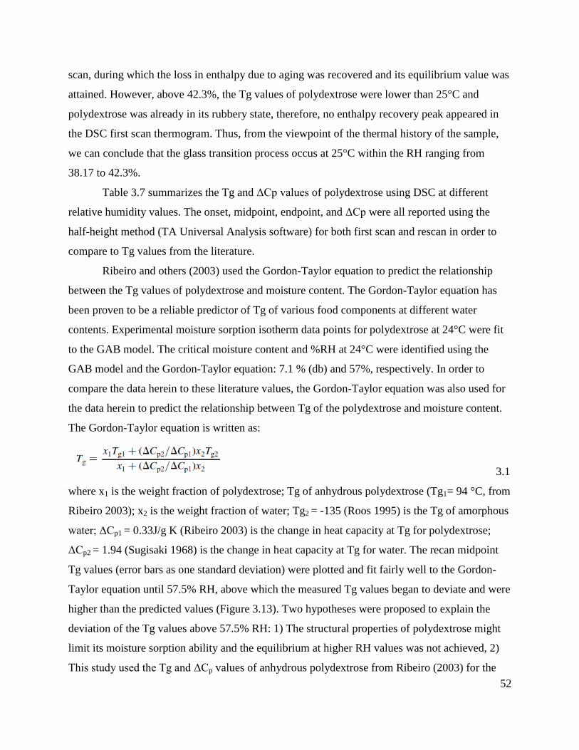
Page 1
INVESTIGATING THE GLASSY TO RUBBERY TRANSITION OF POLYDEXTROSE AND
CORN FLAKES USING AUTOMATIC WATER VAPOR SORPTION INSTRUMENTS, DSC,
AND TEXTURE ANALYSIS
BY
QINGRUISI LI
THESIS
Submitted in partial fulfillment of the requirements
for the degree of Master of Science in Food Science and Human Nutrition
in the Graduate College of the
University of Illinois at Urbana-Champaign, 2010
Urbana, Illinois
Adviser:
Professor Shelly J. Schmidt
Page 2
ii
ABSTRACT
The aim of this study was to investigate the usefulness of automated sorption isotherm
methods for determining the glassy to rubbery transition in a model amorphous food material,
polydextrose. The automated sorption isotherms were obtained from 20 to 40°C at 5°C intervals
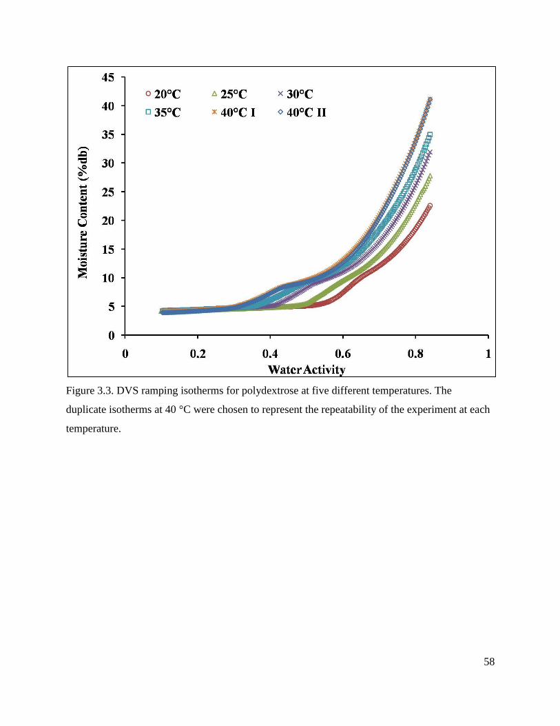
using dynamic vapor sorption (DVS). The DVS ramping isotherm was obtained at a linearly
increasing relative humidity (RH), 2%RH/hr, from 10 to 85%RH. The DVS equilibrium
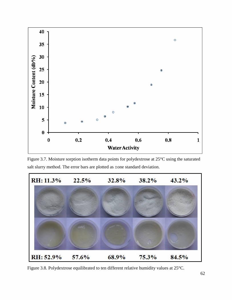
isotherm was obtained at twelve RH values using a dm/dt criterion of 0.0005%. The traditional
saturated salt slurry isotherm was obtained at 25°C using ten saturated salt slurries, with RH
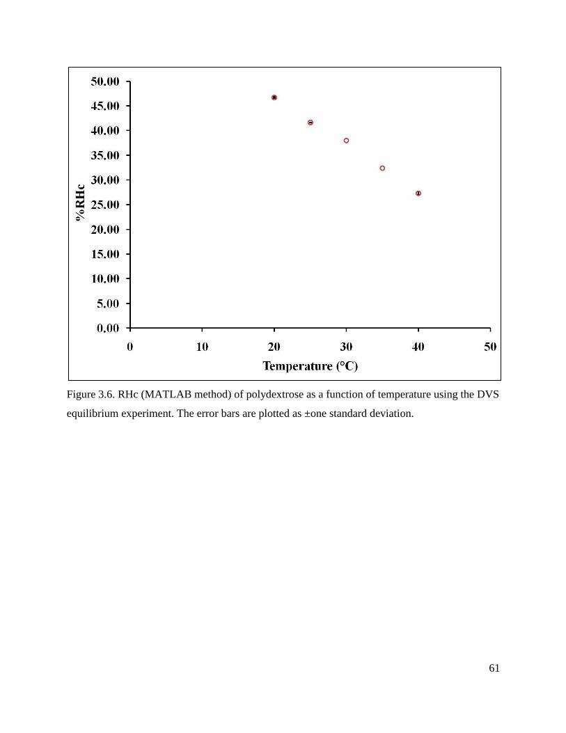
values ranging from 11.3 to 84.3%. The RHc was defined as the %RH that exhibited the fastest
change in slope determined by the maximum of the second derivative of the isotherm curve. The
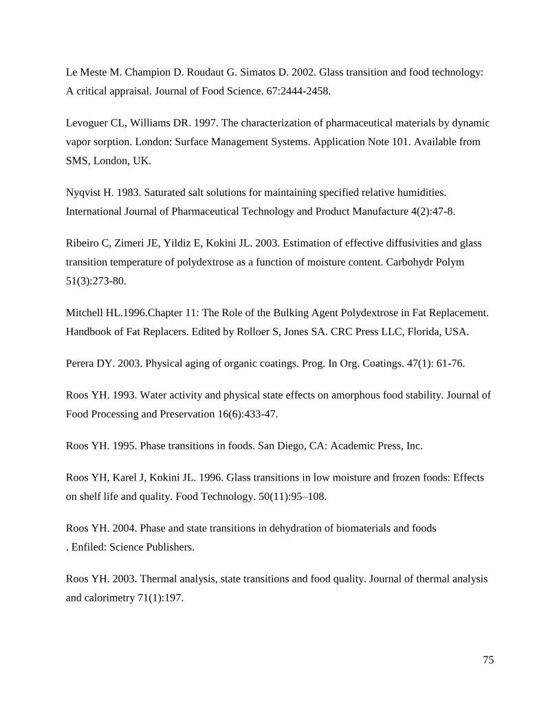
RHc and temperature values were plotted in a state diagram and compared to the differential
scanning calorimetry (DSC) glass transition temperature (Tg) values. As predicted from theory,
RHc values decreased as temperature increased. As plotted on the state diagram, the RHc values
were similar to the DSC Tg values. At the same temperature, the RHc order for the isotherms
was traditional < DVS equilibrium < DVS ramping, with the RHc values depending on the time
the material was exposed to the different RH conditions.
Since the automated sorption isotherm methods showed promise for being a practical tool
to determine the location of the glassy to rubbery transition for polydextrose, the model was
applied to a complex amorphous food system, corn flakes. In addition, textural analysis was
conducted in order to relate the mechanical properties of corn flakes to the glassy to rubbery
transition results from the thermal method and the automated sorption isotherm methods. The
results from corn flakes showed that the AquaSorp dynamic dewpoint (DDI) and DVS ramping
isotherms represented the non-equilibrated isotherm whereas the DVS equilibrium and saturated
salt slurry isotherms represented the equilibrated isotherm. The difference between the isotherms
was most likely associated with the very dense laminated corn flake matrix and the time-
dependent nature of the sorption process. The results from the textural analysis performed at
ambient temperature (25°C) and the saturated salt slurry method were similar, indicating the
glassy to rubbery transition for corn flakes at 25°C occurred at a relative humidity of
37.75±0.64%. The DVS equilibrium method coupled with textural analysis might be a useful
tool to replace the traditional saturated salt slurry method to routinely determine the location of
the glassy to rubbery transition for complex food systems.
Page 3
iii
ACKNOWLEDGEMENTS
I would like to acknowledge and thank my adviser, Dr. Shelly Schmidt. During my two years
study at University of Illinois, I have experienced the excitement of discovering positive results
as well as some difficulties and Dr. Schmidt is the person who always gives me generous
guidance and encouragement. She is patient and supportive in both conducting this project and
helping me make life-changing decisions. I will always remember her theory of research as ―re-
search‖ and have the passion about science research. I have learned so much from her and this
project would never happen without her.
I would also like to thank my committee members, Dr. Nicki Engeseth and Dr. Kent Rausch for
their time and assistance in reviewing my thesis and for their encouragement during my studies.
In addition, I would like to acknowledge Dr. Youngsoo Lee for teaching me texture analysis.
Finally, I would like to thank Dr. Bohn for her guidance and support and the opportunity to being
her teaching assistant. I would like to thank my present and past lab mates, Joo Won, Xiaoda,
Vina, Sarah, and Yiou for their friendship, help and encouragement. Last but not least, I would
like to thank my family for their unconditional love to support me throughout this wonderful
journey.
Page 4
iv
TABLE OF CONTENTS
CHAPTER 1 INTRODUCTION .........................................................................................1
1.1 Rationale and significance .......................................................................................1
1.2 Objectives ................................................................................................................2
1.3 References ................................................................................................................2
CHAPTER 2 LITERATURE REVIEW ..............................................................................3
2.1 Water in foods ..........................................................................................................3
2.1.1 Water activity ..................................................................................................3
2.1.2 Moisture effects on materials ..........................................................................4
2.2 Moisture sorption isotherms ....................................................................................5
2.2.1 Types of isotherms .......................................................................................5
2.2.2 Isotherm prediction models..........................................................................7
2.2.3 Sorption isotherm experimental determination ............................................8
2.2.3.1 Saturated salt slurry method.............................................................8
2.2.3.2 Humidity generating instruments ...................................................10
2.2.3.2.1 Dynamic Vapor Sorption (DVS) instrument ...................10
2.2.3.2.2 AquaSorp Isotherm Generator .........................................12
2.2.3.3 Comparison between saturated salt slurry and humidity
generating methods ........................................................................14
2.3 Glass transition.......................................................................................................15
2.3.1 Physical and mechanical properties of the glass transition ........................15
2.3.2 Critical water activity, moisture content, and the glass transition .............16
2.3.3 Factors that affect the glass transition ........................................................17
2.3.3.1 Water plasticization and antiplasticization ....................................17
2.3.3.2 Molecular weight ...........................................................................19
2.3.4 Applied methods of measuring the glass transition process ......................19
2.4 Mechanical properties ............................................................................................21
2.5 Figures and tables ..................................................................................................23
2.6 References ..............................................................................................................32
CHAPTER 3 DETERMINATION OF THE CRITICAL RELATIVE HUMIDITY
(RHc) FOR POLYDEXTROSE USING A HUMIDITY
GENERATING INSTRUMENT .................................................................39
3.1 Abstract ..................................................................................................................39
3.2 Introduction ............................................................................................................40
3.3 Materials and methods ...........................................................................................43
3.3.1 Materials ....................................................................................................43
3.3.2 Critical relative humidity determined using DVS .....................................43
3.3.2.1 DVS calibration, probe check, and sample ....................................43
3.3.2.3 Ramping sorption isotherm determined using DVS ......................44
3.3.2.3 Equilibrium sorption isotherm determined using DVS .................45
3.3.3 Critical relative humidity determined using saturated salt slurry method ....46
3.3.4 Determination of glass transition temperatures using DSC ..........................47
Page 5
v
3.4 Results and discussion ..........................................................................................48
3.4.1 Critical relative humidity values as a function of temperature using DVS
ramping method ............................................................................................48
3.4.2 Critical relative humidity values as a function of temperature using DVS
equilibrium method .......................................................................................49
3.4.3 Critical relative humidity values from saturated salt slurry method .............50
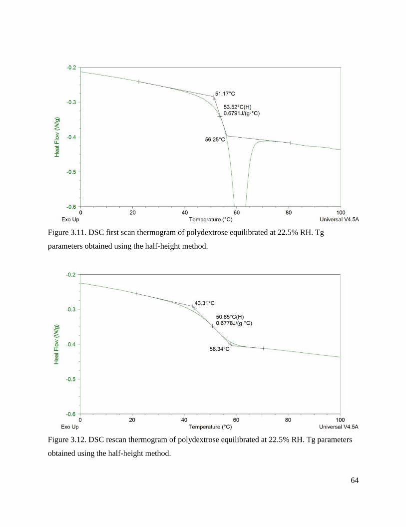
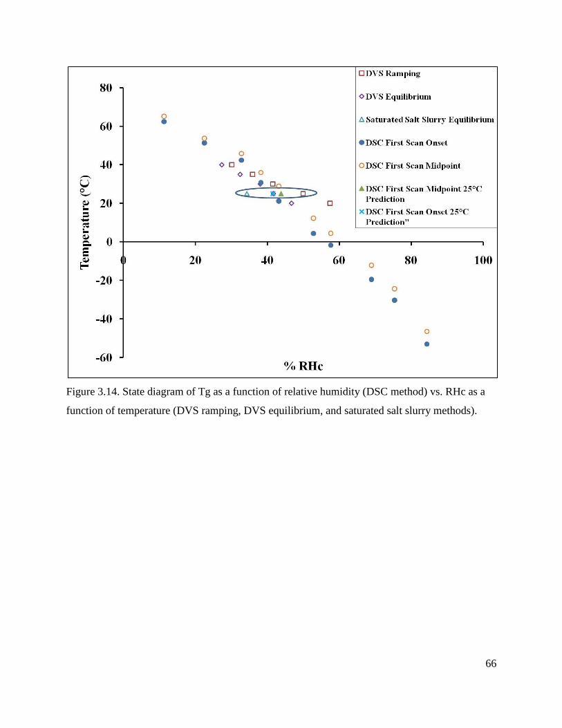
3.4.4 Determination of glass transition using DSC................................................51
3.4.5 Comparison of the relationship between RHc and Tg using different
methods .........................................................................................................53
3.5 Conclusions ...........................................................................................................55
3.7 Figures and tables .................................................................................................56
3.6 References .............................................................................................................73
CHAPTER 4 CHARACTERIZATION OF THE SORPTION BEHAVIOR OF CORN
FLAKES USING HUMIDITY GENERATING INSTRUMENTS,
DIFFERENTIAL SCANNING CALORIMETRY (DSC), AND
TEXTURAL ANALYSIS ............................................................................77
4.1 Abstract ..................................................................................................................77
4.2 Introduction ............................................................................................................78
4.3 Materials and methods ...........................................................................................85
4.3.1 Materials ....................................................................................................85
4.3.2 Critical relative humidity determination ....................................................85
4.3.2.1 DVS ramping and equilibrium methods ...........................................85
4.3.2.2 AquaSorp dynamic dewpoint isotherm (DDI) method .....................87
4.3.2.3 Saturated Salt Slurries method..........................................................87
4.3.3 Determination of glass transition temperatures using DSC .......................88
4.3.4 Textural analysis ........................................................................................89
4.4 Results and discussion ...........................................................................................90
4.4.1 Critical relative humidity (RHc) values as a function of temperature
from DVS ramping method .......................................................................90
4.4.2 RHc values as a function of temperature from DVS equilibrium method .90
4.4.3 RHc values as a function of temperature from DDI method .....................92
4.4.4 RHc values from saturated salt slurry method ...........................................92
4.4.5 Determination of glass transition using DSC.............................................93
4.4.6 Effect of increasing % RH on hardness and energy input .........................95
4.4.7 Comparison of the relationship among thermal method, humidity
generating methods, and textural analysis .................................................96
4.5 Conclusions ............................................................................................................99
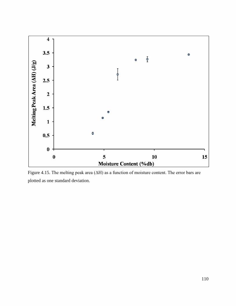
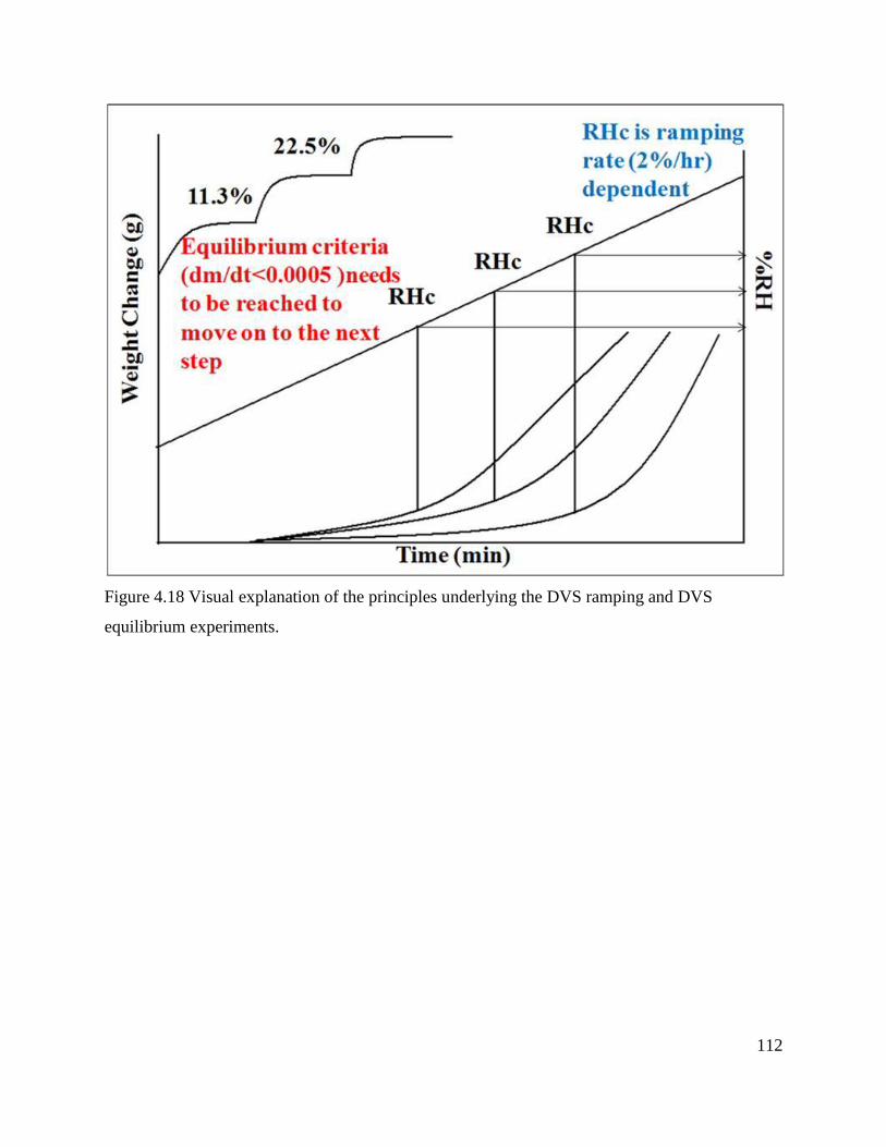
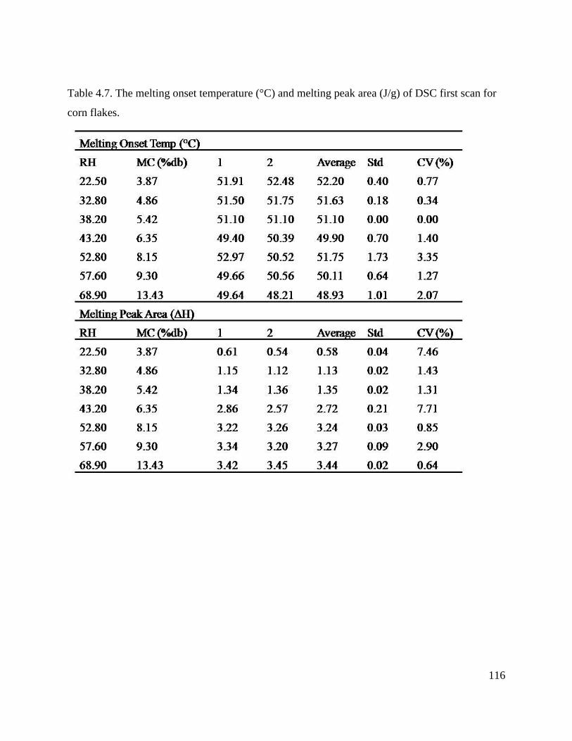
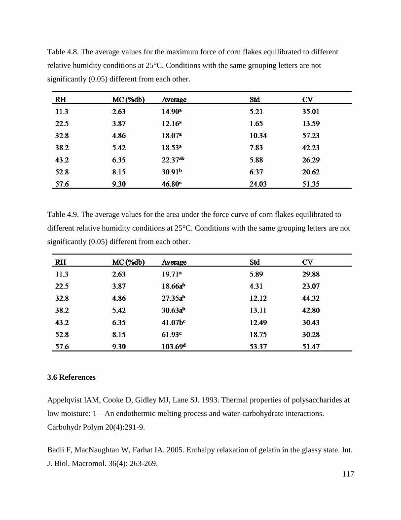
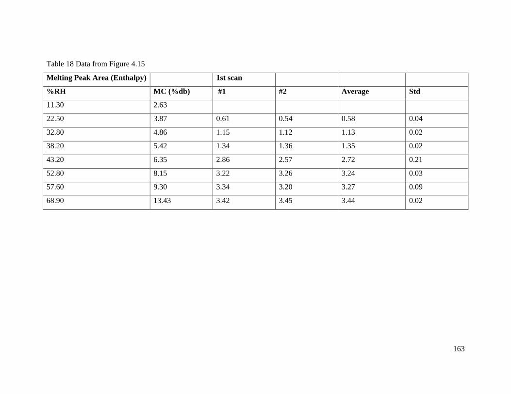
4.6 Figures and tables ................................................................................................100
4.7 References ............................................................................................................117
APPENDIX. ...............................................................................................................121
Page 6
1
CHAPTER 1 INTRODUCTION
1.1 Rationale and significance
The introduction of the food polymer science (FPS) approach to study food ingredients
and systems, pioneered by Slade and Levine (e.g., 1987 and 1991), has revolutionized the topic
of moisture management in food systems and has been the impetus for numerous research studies
exploring the FPS approach for the assessment of food quality, stability, and safety. One of the
key elements of the FPS approach is the glass transition and its relationship to the processibility,
product properties, quality, stability, and safety of food systems. When the material transforms
from the glassy to the rubbery state, the molecules become mobile, which can alter food structure
and microstructure, crystallization, rates of diffusion, stabilization of microbial cells and spores,
and chemical and biochemical reactions.
The glassy to rubbery transition in amorphous materials can be described either by a glass
transition temperature (Tg) at a specified moisture content or a critical relative humidity (RHc) at
a specified temperature. Traditionally, thermal methods, such as differential scanning
calorimetry (DSC), are used to determine the glassy to rubbery transition. However, two major
disadvantages of using DSC for measuring Tg are: 1) low sensitivity and 2) the possible
occurrence of multiple thermal events (e.g., starch gelatinization, protein denaturation) that may
overlap or interfere with determination of the glass transition. Besides standard thermal methods,
the glass transition process can also be detected by changing the relative humidity at a constant
temperature. Since the water sorption isotherm is already a vital requirement of food safety and
quality assurance, it would be highly desirable if a direct, practical means of determining the Tg
from water vapor sorption behavior of complex amorphous food materials could be established.
Newly developed automated sorption isotherm instruments have the advantages of high
resolution data capacity and short experimental times compared to the saturated salt slurry
method. Studies have been done to prove the ability of automated sorption isotherm instruments
to detect the glassy to rubbery transition (Burnett and others 2004; Yuan 2009) for amorphous
food materials. However, no published research was found using automated sorption isotherm
instruments at various temperatures compared to the saturated salt slurry method and the thermal
method for the purpose of investigating the glassy to rubbery transition. Thus, polydextrose was
used to investigate the hypothesis that newly developed automated sorption isotherm methods,
Page 7
2
coupled with the saturated salt slurry method, can be used to detect the glassy to rubbery
transition. Corn flakes will be chosen as a model complex food system to further investigate the
hypothesis whether newly developed automated sorption isotherm instruments can be utilized as
a tool to routinely determine the glassy to rubbery transition.
1.2 Objectives
The major objectives of this research were to: 1) investigate the usefulness of automated
sorption isotherm methods for determining the glassy to rubbery transition in a model amorphous
food material, polydextrose, and 2) apply the model to a complex amorphous food system, corn
flakes, and relate the mechanical properties of corn flakes to the glassy to rubbery transition
results from the thermal method and the automated sorption isotherm methods.
1.3 References
Burnett DJ, Thielmann F, Booth J. 2004. Determining the critical relative humidity for moisture-
induced phase transitions. Int J Pharm 287(1-2):123.
Slade L, Levine S. 1987. Recent advances in starch retrogradation. In Industrial Polysaccharides
– The Impact of Biotechnology and Advanced Methodologies. SS Stivala, V. Crescenzi, and
ICM Dea, Eds, Gordon and Breach Science Publishers, New York, p. 387-430.
Slade L, Levine H. 1991. Beyond water activity: recent advances based on an alternative
approach to the assessment of food quality and safety. Crit Rev Food Sci Nutr 30(2-3):115.
Yuan X. 2009. Investigation of the relationship between the critical relative humidity and the
glassy to rubbery transition in polydextrose. [Thesis]. Urbana, IL: University of Illinois at
Urbana-Champaign.
Page 8
3
CHAPTER 2. LITERATURE REVIEW
2.1 Water in foods
Water is the most abundant, unique, and necessary substance on the face of earth
(Schmidt 2004). It is the only substance on the planet that commonly exists in all three physical
states: solid, liquid, and gas. Water influences the chemical and microbial stability, physical
properties, (i.e., texture and appearance, phase transitions), and sensory properties of foods. All
of the factors mentioned above determine the quality and safety of foods.
2.1.1 Water activity
The concept of substance ―activity‖ was derived by Gilbert N. Lewis (1907) from the
laws of equilibrium thermodynamics and was described in detail by Lewis and Randell (1923)
(Schmidt 2004). Each component has a chemical potential (µ), which represents the free energy
added to the system per mole of the compound. In a food system, the chemical potential of water
can be expressed in the following equation:
2.1
Where is the chemical potential of pure water in a standard state, R is the universal gas
constant, T is temperature, and aw is the activity of water. Because the chemical potentials of
water distributed in two phases must be equal, the aw of a food can be measured by the partial
vapor pressure of water above the food (p) divided by the vapor pressure of pure water (po) at the
same temperature and atmospheric pressure (Scott 1957):
2.2
Thus, the aw of a food can be expressed a percent relative humidity (%RH) divided by
100. There are two main assumptions underlying the definition of aw: 1) the food system must be
in thermodynamic equilibrium, 2) the temperature and atmospheric pressure must be constant
(Schmidt 2004). Most food systems, which experience physical, chemical, microbiological
changes over time, are non-equilibrium systems. However, the concept of aw has been proven to
be an extremely useful and practical tool in both the food industry and in food science research
(Franks 1991). Unlike total moisture content, which does not indicate the water availability
associated with biological, chemical, and physical reactions, aw can be used as an empirical
Page 9
4
parameter to correlate with microbial growth and chemical reactions rates (Fennema 1996,
Christen 2000).
There are a variety of techniques that can be used to measure aw, including vapor pressure
manometer, hygroscopicity of salts, hygrometric instruments (i.e., resistance, capacitance, and
dew point), and isotherm and isopiestic methods (Schmidt 2004).
2.1.2 Moisture effects on materials
There are five major mechanisms for water-solid interactions in solid food materials:
adsorption of water vapor on to the surface, crystal hydrate formation, deliquescence, capillary
condensation, and absorption of water vapor into the bulk structure. Solid food materials can
generally be divided into two categories: crystalline solids and amorphous solids.
For the crystalline solids, there are three major mechanisms of water-solid interactions:
adsorption of water vapor on to the solid air-interface, crystal hydrate formation, and
deliquescence (Ahlneck and Zografi 1990). If the material contains microvoid spaces, capillary
condensation will occur, which is the fourth mechanism. Capillary condensation can be partially
explained by the ―ink-bottle theory‖ (McBai 1935; Rao and Das 1968). It is also one of the
theories for the explanation of hysteresis. Crystal hydrates are characterized by the penetration of
water molecules into the crystal lattice and hydrogen bonded to certain groups with a specific
stoichiometry (Byrn 1982). Crystalline solids posses close packing and a high degree of order
and, thus, adsorb only a small amount of moisture onto the surface of the crystalline structure
until reaching the deliquescence point, defined as the critical relative humidity (RH0). RH0 is
unique to each crystalline material and is a function of temperature (Van Campen 1983).
For amorphous solids, there are two major mechanisms of water-solid interactions:
adsorption of water vapor on to the surface and absorption of water vapor into the bulk
structureIn general, amorphous solids are in a thermodynamically pseudo-stable state compared
to the crystalline solids and are lacking in molecular order (Barbosa-Canovas 2007). The amount
of moisture sorbed by amorphous solids is typically greater than crystalline solids below their
critical RH0 (Kontny and Zografi 1995). In contrast to adsorption, where the amount of water
taken up depends on the available surface area, water uptake by amorphous materials is
predominantly determined by the total mass of amorphous content (Ahlneck and Zografi 1990).
Amorphous solids, depending on their water activity and temperature, can exist in two states: the
Page 10
5
glassy state and the rubbery state. Properties of solids change when they transition from the
glassy state to the rubbery state. We define this process as the glass transition process, which can
be achieved by increasing temperature, relative humidity, or both. It is important for processing
and storage of amorphous materials to determine the critical condition, such as temperature and
relatively humidity, where the glass transition occurs (Burnett 2004). Different properties of the
two states can also influence sorption isotherms (Barbosa-Canovas 2007). There are a variety of
amorphous food products in the industry, such as breakfast cereal and spray dried powders. The
shelf stability and textural properties of amorphous food products can be greatly affected by their
physical state, water mobility, and water-solid interactions.
2.2 Moisture sorption isotherms
Moisture sorption isotherms illustrate the steady-state amount of water held by the food
solids as a function of aw or %RH at constant temperature (Labuza 1968). Moisture vapor
sorption by foods depends on many factors, including chemical composition, physical-chemical
state of the ingredients, and physical structure (Barbosa-Canovas 2007). It is a valuable tool for
the food industry because aw can be predicted at a given moisture content to control water
migration and increase stability.
2.2.1 Types of isotherms
Each food exhibits a unique set of sorption isotherms at different temperatures (Fellows
2000), but most sorption isotherms have a characteristic sigmoidal shape, similar to that shown
in Figure 2.1 (Fennema 1996). Region I (aw<0.25) represents monolayer water which is strongly
sorbed, unfreezable, and not easily removed by drying. The water in this region interacts most
strongly with the solids and is least mobile. The Brunauer-Emmet-Teller (BET) monolayer
moisture content is located at the end of Region I, which is considered to be a monolayer of
water bound to specific polar sites on the dry solids. Region II (0.25<aw<0.75) represents water
sorbed (both adsorption and absorption can occur in this region) in multilayers within foods and
solutions of soluble components. It is still slightly less mobile than bulk water. As water is added
in the vicinity of the low-moisture end of Region II, it exerts a significant plasticizing action on
solutes, lowers their glass transition temperatures and causes incipient swelling of the solid
matrix (Yu 2007). The third region is bulk or ―free‖ water, which is freezable and is easily
Page 11
6
removed by drying. It is also available for microbial growth and enzyme activity. Region III
water is referred to as bulk-phase water.
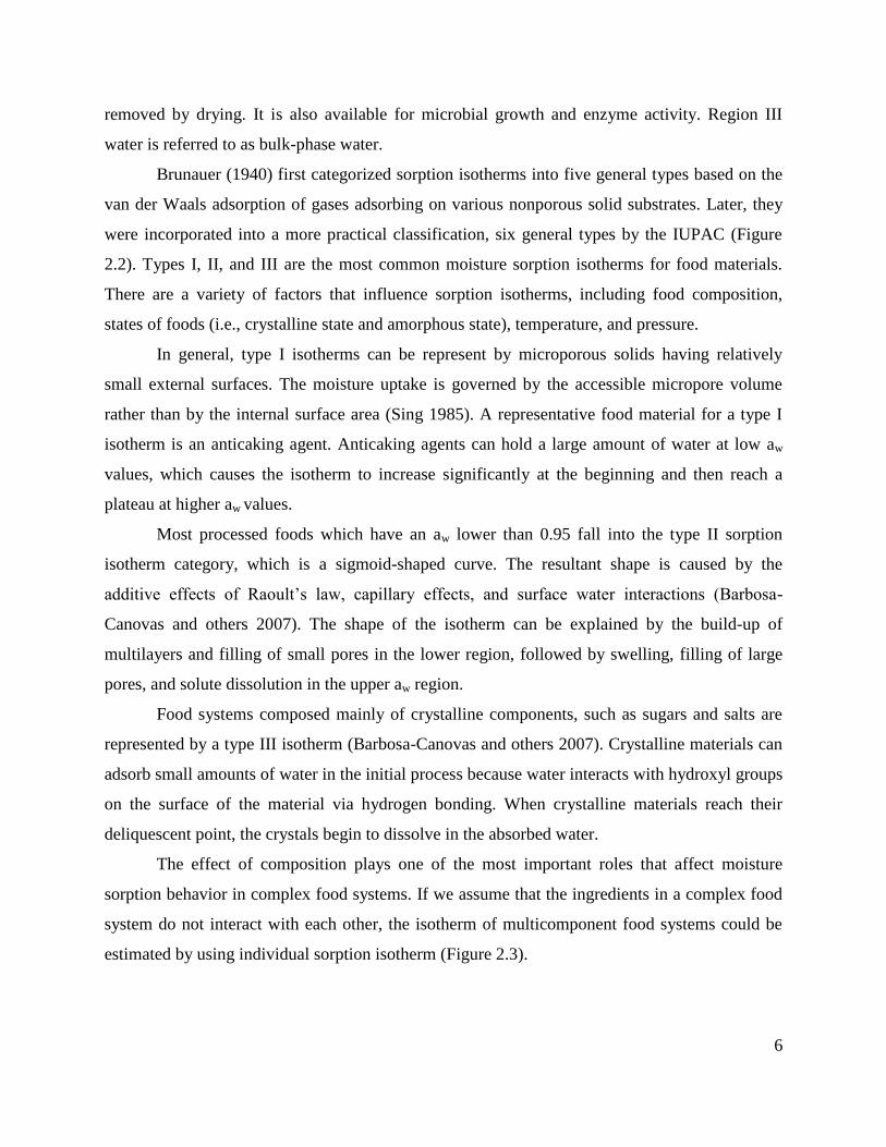
Brunauer (1940) first categorized sorption isotherms into five general types based on the
van der Waals adsorption of gases adsorbing on various nonporous solid substrates. Later, they
were incorporated into a more practical classification, six general types by the IUPAC (Figure
2.2). Types I, II, and III are the most common moisture sorption isotherms for food materials.
There are a variety of factors that influence sorption isotherms, including food composition,
states of foods (i.e., crystalline state and amorphous state), temperature, and pressure.
In general, type I isotherms can be represent by microporous solids having relatively
small external surfaces. The moisture uptake is governed by the accessible micropore volume
rather than by the internal surface area (Sing 1985). A representative food material for a type I
isotherm is an anticaking agent. Anticaking agents can hold a large amount of water at low aw
values, which causes the isotherm to increase significantly at the beginning and then reach a
plateau at higher aw values.
Most processed foods which have an aw lower than 0.95 fall into the type II sorption
isotherm category, which is a sigmoid-shaped curve. The resultant shape is caused by the
additive effects of Raoult’s law, capillary effects, and surface water interactions (Barbosa-
Canovas and others 2007). The shape of the isotherm can be explained by the build-up of
multilayers and filling of small pores in the lower region, followed by swelling, filling of large
pores, and solute dissolution in the upper aw region.
Food systems composed mainly of crystalline components, such as sugars and salts are
represented by a type III isotherm (Barbosa-Canovas and others 2007). Crystalline materials can
adsorb small amounts of water in the initial process because water interacts with hydroxyl groups
on the surface of the material via hydrogen bonding. When crystalline materials reach their
deliquescent point, the crystals begin to dissolve in the absorbed water.
The effect of composition plays one of the most important roles that affect moisture
sorption behavior in complex food systems. If we assume that the ingredients in a complex food
system do not interact with each other, the isotherm of multicomponent food systems could be
estimated by using individual sorption isotherm (Figure 2.3).
Page 12
7
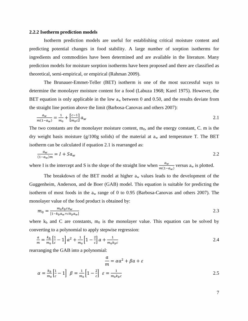
2.2.2 Isotherm prediction models
Isotherm prediction models are useful for establishing critical moisture content and
predicting potential changes in food stability. A large number of sorption isotherms for
ingredients and commodities have been determined and are available in the literature. Many
prediction models for moisture sorption isotherms have been proposed and there are classified as
theoretical, semi-empirical, or empirical (Rahman 2009).
The Brunauer-Emmet-Teller (BET) isotherm is one of the most successful ways to
determine the monolayer moisture content for a food (Labuza 1968; Karel 1975). However, the
BET equation is only applicable in the low aw between 0 and 0.50, and the results deviate from
the straight line portion above the limit (Barbosa-Canovas and others 2007):
2.1
The two constants are the monolayer moisture content, m0, and the energy constant, C. m is the
dry weight basis moisture (g/100g solids) of the material at aw and temperature T. The BET
isotherm can be calculated if equation 2.1 is rearranged as:
2.2
where I is the intercept and S is the slope of the straight line when
versus aw is plotted.
The breakdown of the BET model at higher aw values leads to the development of the
Guggenheim, Anderson, and de Boer (GAB) model. This equation is suitable for predicting the
isotherm of most foods in the aw range of 0 to 0.95 (Barbosa-Canovas and others 2007). The
monolayer value of the food product is obtained by:
2.3
where kb and C are constants, m0 is the monolayer value. This equation can be solved by
converting to a polynomial to apply stepwise regression:
2.4
rearranging the GAB into a polynomial:
2.5
Page 13
8
Finally Kb, m0, and C can be solved by using the binomial equation. The GAB model is
similar to the BET equation with the assumption of localized physical adsorption in multilayers
with no lateral interactions (Barbosa-Canovas and others 2007).
Although the BET and GAB models are apparently useful in explaining various stability
mechanisms, they are not always compatible with the other moisture sorption phenomenon,
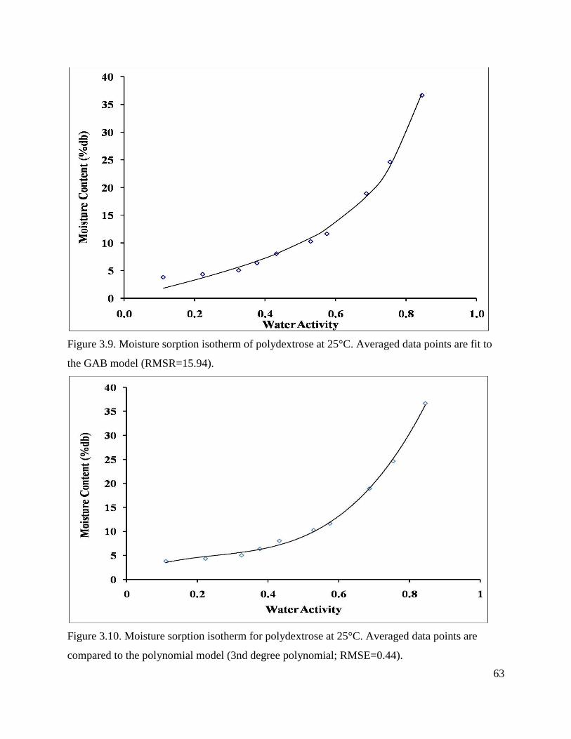
which might be supported by empirical equations. The polynomial equation describing sorption
isotherms was proposed by Alam and Shove (1973), also termed the Double Log Polynomial
(DLP) by Decagon Devices (2007):
2.6
Although the m versus aw data are used to determine the parameter constants in the polynomial
model and they fit, the model constants do not have any theoretical meaning; however, it is
useful modeling tool.
2.2.3 Sorption isotherm experimental determination
The moisture sorption isotherm of a food is obtained from the equilibrium moisture
contents determined at several aw values at constant temperature. Food sorption isotherms are
widely used in food processing, especially in drying, mixing, packaging, and for controlling
spoilage by microorganisms (Lewicki 2003; Kitic 1986). Barbosa-Canovas and others (2007)
summarized the determination of moisture sorption isotherm into two ways: 1) food samples that
are either dried (absorption), hydrated (desorption), or native (working) are placed in controlled
humidity chambers at constant temperature and the weight is measured until equilibrium (e.g.,
saturated salt slurry method and humidity generating instruments); 2) a series of samples with
varied moisture contents are established by adding or removing moisture, and then, aw and water
content are measured (e.g., fast isotherm method).
2.2.3.1 Saturated salt slurry method
The saturated salt slurry method has been traditionally used to adjust the humidity of the
air in order to establish a required humidity value in a sealed container. At a constant
temperature, the solubility of a saturated salt slurry remains constant, which gives the chamber
the ability to maintain a constant relative humidity. Thus, food samples will be brought to
equilibrium with the surrounding environment of known water activity (Lewicki 2003) within
Page 14
9
days or months, depending on the sample structure, the movement of surrounding air, the sample
size, the pressure of the air inside the chamber, the chamber size, and the initial aw of the food
sample. Greenspan (1977) studied 28 saturated salt slurries, which encompassed a range of
relative humidity values from 3% to 98%, at seven temperatures ranging from 10 to 40°C at an
increment of 5°C. In order to obtain a representative isotherm, an appropriate series of saturated
salts should be selected to cover the desired isotherm range (Greenspan 1977).
When making a saturated salt slurry, the researcher should be careful and cautious to
reduce the variation (Labuza 1984). The solution should be a slurry with excess crystals present
to cover the entire bottom of the container using pure salt and water. The excessive crystals can
act as a buffer to dissolve into the solution for absorbing moisture when the aw of food samples is
higher than the relative humidity of the chamber, or precipitate crystals from the solution for
providing moisture when the aw of food samples is lower than the relative humidity of the
chamber. Eventually, the sample will reach the aw of the saturated salt. The slurry should be
made at or above the temperature at which the isotherm is to be carried out because the solubility
of many salts increase significantly with temperature and the excess salt may not be sufficient
(Labuza 1984). In addition, some salts are potentially toxic if they contaminate the food being
humidified. The researcher should be extremely cautious in selecting the salt regarding of
sensory testing to prevent possible food poisoning, flavor deterioration, and lipid oxidation
(Labuza 1984, Yu 2007).
The saturated salt slurry method has the advantage of generating accurate aw values as a
function of temperature, as well as providing the sample the opportunity to reach its true
equilibrium due to relatively long equilibration times. In addition, many samples can be
equilibrated to desire relative humidity at once with a relatively low initial cost. However,
Lewicki (2003) showed that the disturbance of equilibrium can be caused by reopening the
desiccators. The disadvantages of saturated salt slurry method using desiccators have been
summarized (Levoguer 1997): 1) the lengthy period of time it takes the product to achieve
equilibrium, 2) the difficulty of obtaining accurate measurements due to exposure of the sample
to an environment which often has a different relative humidity, 3) the requirement of using large
sample sizes to obtain a measurement, and 4) it is time-consuming and labor intensive.
Page 15
10
2.2.3.2 Humidity generating instruments
Compared to the saturated salt slurry method, newly developed humidity generating
instruments have the ability to generate sorption isotherms in a relatively short period of time
due to the dynamic environment, and they are automated. Some commercialized humidity
generating instruments are (Mermelstein, 2009): Dynamic Vapor Sorption instrument (Surface
Management Systems, London, UK), IGA-Sorp (Hiden Analytical, Warrington, England), VTI
and Q5000SA (TA Instruments, Delaware, USA), Cisorp Water Sorption Analyzer (CI
Electronics Ltd, Salisbury, UK), SPS Moisture Sorption Analyzers (Project Messtechnk, Ulm,
Germany), Hydrosorb™ 1000 Water Vapor Sorption Analyzer (Quantachrome Instruments,
Boynton Beach, FL), and AquaSorp Isotherm Generator (Decagon Devices Inc., Pullam, WA).
The DVS instrument and AquaSorp Isotherm Generator have been used in various
research studies (Buckton and others 1995; Mackin and others 2002; Bohn and others 2005;
Burnett and others 2006; Schmidt and Lee 2009; Schmidt and Lee 2009; Spackman and Schmidt
2009; Yuan 2009) and were chosen for this study since they are the main instruments used in the
Schmidt Lab.
2.2.3.2.1 Dynamic Vapor Sorption (DVS) instrument
The DVS Intrinsic is the latest dynamic gravimetric water sorption analyzer from Surface
Measurement Systems (London, UK). The instrument was specifically designed to meet the
needs of the small to mid-sized laboratories and plants and combines ease of use with a low
capital investment and maintenance burden (Surface Measurement Systems website). It is a fully
automated humidity generating instrument via control from a dedicated laptop computer and
utilizes the same principle as the DVS1000/DVS2000, which was developed in 1994 by Surface
Management Systems (London, UK). The instrument is designed to accurately measure the
sample weight change as it absorbs/desorbs moisture from air with a known relative humidity at
a constant temperature. Selected relative humidity values are generated by mixing accurate
amounts of selected dry and saturated air or nitrogen flows using sensitive mass flow controllers.
The system has a relative humidity sensor to verify its humidity generating performance and a
temperature probe. The sample mass reading is measured by an ultra-sensitive microbalance,
which reflects the vapor sorption behavior of the sample. A constant flow rate of dry nitrogen
gas and a head temperature (40 °C) are used to prevent potential microbalance vapor
Page 16
11
condensation. The microbalance can measure a mass change of up to 150 mg without the need of
a counterweight with a resolution of ±0.1µg. The instrument has the capacity to perform in a
temperature ranging from 20 to 40 °C.
The DVS instrument has been utilized to study the sorption behavior of amorphous and
crystalline materials. Buckton and others (1995) studied the absorption/desorption properties of
mixtures of amorphous lactose and crystalline α-lactose monohydrate. The experiments carried
out by DVS instruments showed a higher weight gain due to absorption into the amorphous
region followed by weight loss because of recrystallization in the first sorption process. On
desorption, the residual water indicated the transformation of amorphous material into
monohydrate form, which can be utilized as an approximate quantification of the original
amorphous content of the sample. Yu and others (2007) investigated the moisture sorption
behavior of amorphous sucrose using DVS instrument and found that moisture-induced
crystallization onset time decreased as %RH increased. In addition, crystalline content of
amorphous sucrose had a significant impact on the pseudo-sorption isotherm. As crystalline
content increases, the equilibrium moisture content at the same relative humidity decreased.
Besides crystalline content, the induction times for crystallization indicated a strong relationship
with both temperature and humidity (Burnett and others 2006).
For comparison, other techniques have been applied and have shown good agreement
with the DVS instrument. Burnett and others (2004) studied the glass transition and
crystallization processes in amorphous or partially amorphous materials at various temperatures
and ramping rates using DVS instrument. The results were verified using inverse gas
chromatography (IGC) and proved that the DVS instrument could be used for determining the
critical storage and processing relative humidity for spray-dried lactose and salbutamol sulfate.
Mackin and others (2002) illustrated that both the DVS and microcalorimeter were able to detect
the amorphous content of a benzyl ether derivative. Results from the DVS and microcalorimeter
showed an excellent agreement. Bohn and others (2005) studied the flavor release of an artificial
cherry duratrome at various relative humidity values using the DVS techniques and fast gas
chromatography-flame ionization detection.
Page 17
12
2.2.3.2.2 AquaSorp Isotherm Generator
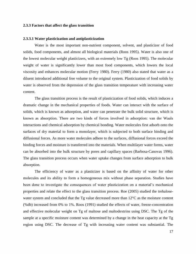
The AquaSorp Isotherm Generator (Figure 2.5) is an automatic moisture sorption
isotherm generator which rapidly creates detailed adsorption and desorption isotherm curves
(AquaSorp Users Manual, 2007), which are called Dynamic Dewpoint Isotherms. The sample
can be wetted by saturated wet air or dried by flowing dry air from a desiccant tube. Moisture
content is measured by tracking the weight change using a high precision magnetic force balance
and aw is determined using a chilled-mirror dewpoint senor. A water reservoir is used to ensure
humidity saturation and minimize temperature fluctuations. The specifications of AquaSorp are
given in Table 2.1.
The AquaSorp must be thermally equilibrated to a desired test temperature before
initiating a new test. The instrument temperature is set to 25°C as default and a temperature other
than 25°C will need additional equilibration time. Since the AquaSorp uses the chilled mirror
dewpoint technique, which is a primary measurement method of relative humidity, no calibration
is necessary; however, frequent linear offset verification should be performed to ensure the
accuracy of the instrument. Linear offset can be checked by using a salt solution and distilled
water. Verification standards are specially prepared salt solutions which have a specific molality
and water activity that is constant and accurately measurable (AquaSorp Users Manual, 2007).
Decagon recommends that the AquaSorp should be checked with a high and low salt standard,
preferably the NaCl and LiCl standards. The salt solution aw values, as a function of temperature,
are listed in Table 2.2.
The AquaSorp generates isotherms with numerous data points (>usually greater than 75
for a full isotherm) and faster than other isotherm methods because it does not require the sample
to equilibrate to a known humidity value. Instead, aw and moisture content are measured during
the wetting or drying process. For desorption isotherms, dry air from a desiccant tube flows
across the sample to carry moisture away. For absorption isotherm, saturated air generated from
the water reservoir flow across the sample. After a short period of time, airflow is stopped and a
snapshot of the sorption process is taken by directly measuring the aw and weight. The
advantages of this method are short waiting time, high data resolution, low supply cost (only
water and desiccant are needed). However, isotherms generated by the AquaSorp method might
be different from the saturated salt slurry isotherms or other humidity generating instrument
Page 18
13
isotherms, such as DVS isotherms, because it does not require the sample to equilibrate to the
environment.
According to AquaSorp Manual (2007), for samples with fast vapor diffusion rates,
penetration by water vapor in to the whole sample is rapid and the isotherm from the AquaSorp
method is comparable to other methods. For samples with slow vapor diffusion rates, the
moisture has not had time to be completely adsorbed by the sample, or desorbed from the sample,
so that the instrument only measures the appearance of vapor equilibrium in the headspace
during aw analysis. As a result, the AquaSorp method may report lower moisture contents during
adsorption and higher moisture contents during desorption at the same water activity on an
isotherm curve than isotherms constructed using other methods. A better agreement might be
achieved by reducing the sample size and lowering the wet or dry air flow rate to allow more
moisture penetration into slow diffusing samples.
Yuan (2009) studied the effect of AquaSorp flow rates on the critical relative humidity
(RHc), that is, the RH that induces the glassy to rubbery transition. The higher flow rates yielded
higher RHc values, which indicated that the bulk aw was not able to keep up with the surface aw
and the system was not in an equilibrium state. A linear extrapolation was conducted on the RHc
values between flow rates 50 and 150 ml/min to obtain the RHc0 values at a flow rate of zero.
Schmidt and Lee (2009) compared the Dynamic Dewpoint isotherms to saturated salt slurry
isotherms for five materials – dent corn starch, isolated soy protein, microcrystalline cellulose,
crystalline sucrose, and corn flakes. The results showed that Dewpoint isotherms exhibited
similar sorption behavior to the saturated salt slurry isotherms, except for corn flakes, which
generated a low moisture content between 0.4 and 0.7 aw. They attributed the difference in the
isotherms to the slow diffusion of water into the very dense laminated corn flake matrix. Shands
and Labuza (2009) also studied the isotherm differences among the Dewpoint isotherm method,
the dynamic gravimetric method (DVS), and the static gravimetric (traditional saturated salt) by
selecting samples that represent isotherm types 1, 2, and 3. They found that the Dewpoint
method when applied to type 1 and type 3 materials generated an isotherm comparable to
traditional methods. The result was similar to Schmidt and Lee (2009) that the Dewpoint method
when applied to type 2 materials, corn flakes, typically generated isotherms with lower moisture
sorption in the mid to low water activity region as compared to the dynamic gravimetric and
static gravimetric method. In addition, they reported that grinding the corn flakes increased the
Page 19
14
surface area available for sorption and decreased the distance for diffusion, which produced a
higher moisture sorption and was comparable to isotherms from the gravimetric methods.
Spackman and Schmidt (2009) also used the dynamic dew point isotherm method as a tool
coupled with textural analysis to analyze the water sorption behavior of sugar gum pastes.
2.2.3.3 Comparison between saturated salt slurry and humidity generating methods
The main advantages of the newly developed humidity generating instruments, such as
the DVS and AquaSorp Isotherm Generator, compared to the saturated salt slurry method are: 1)
smaller sample size and faster equilibration time, 2) near continuous collection of data points, 3)
automated system which has an %RH and temperature controlled environment (Yu 2007).
With the noticeable advantages of DVS technology, some researchers evaluated the speed
of experiments and the accuracy of isotherms generated using the DVS technology compared to
the saturated salt slurry method. Teoh and others (2001) compared the isotherm of cornmeal
using the DVS2000 to the Proximity Equilibration Cell (PEC) method (Lang and others 1981),
which is similar to the saturated salt slurry method but uses a small chamber to decrease
equilibration time. They concluded that the DVS technology can produce rapid isotherms and
provide an isotherm matching traditional results in a fraction of the time. Using a small sample
size and a flow of humidified air as opposed to static equilibration, equilibration times for the
DVS are radically reduced to as short as 1 day, depending upon how many aw points are
specified and selected for equilibration criteria, whereas the PEC method might take up to 22
days depending on the sorption behavior of the food materials.
Arlabosse and others (2003) compared the differences between the saturated salt slurry
methods and the DVS based on the apparent diffusion coefficient. Isotherms generated by these
two method showed good agreement if the apparent diffusion coefficient was higher than
10-9
m2/s. With an apparent diffusion coefficient higher than 10
-9m
2/s, water was mainly adsorbed
at the surface of the material and diffusion inside was negligible. The effect of the dynamic
environment was minimized because of the relative easiness of the diffusion process. However,
with a low apparent diffusion coefficient, it was difficult to reach thermodynamic equilibrium in
the saturated salts method because of the static environment. Thus, when internal diffusion
controls moisture sorption, the DVS method was a better choice for reaching the thermodynamic
equilibrium. However, this research study did not consider the factor of time when comparing
Page 20
15
the two methods. Although the DVS has the advantage of a dynamic environment, the saturated
salt slurry method allows a much longer period of time for the material to reach equilibrium
regardless the difference of diffusion coefficients. Yu (2007) obtained isotherms of various food
ingredients (dent corn starch, isolated soy protein, microcrystalline cellulose, crystalline sucrose,
and corn flakes) using five methods, DVS1000, DVS2000, desiccator, PEC, and the fast
isotherm method. Very good agreement was found among the DVS1000, DVS2000, desiccator,
and PEC methods.
Shands and Labuza (2009) studied the isotherm differences among Dewpoint isotherm
method, dynamic gravimetric method (DVS), and static gravimetric (traditional saturated salt) by
selecting samples which represent isotherm types 1, 2, and 3. They found that the Dewpoint
method when applied to type 1 and type 3 materials generated an isotherm comparable to
traditional methods. However, when applied to type 2 materials, such as breakfast cereals, it
showed a lower moisture sorption in the mid to low aw region compared to traditional methods.
The difference was attributed to slow diffusion rates and was improved by increasing the surface
area by decreasing particle size via grinding.
The saturated salt slurry and the newly developed humidity generating technology are the
two main types of method used to obtain sorption isotherm measurements (Yu 2007). However,
the choice of one method rather than another one to determine a sorption isotherm is still not
very easy (Arlabosse and others 2003). There are many factors to be considered, such as DVS
equilibrium criteria (dm/dt), equilibration time, diffusion coefficient, capital investment, and
material structure and porosity. Investigating more food products with the consideration of these
critical factors will test the reliability of the new technology while addressing the potential
problems in the traditional method.
2.3 Glass Transition
2.3.1 Physical and mechanical properties of the glass transition
Amorphous food materials are in a non-equilibrium state, which can be greatly affected
during processing and storage (Troy 1930; White 1966; Levine 1986; Roos 1991). An
amorphous material can either exist in the glassy state or in the rubbery state, which depends on
its composition, temperature, and time. The term glass transition temperature refers to the
Page 21
16
temperature at which the glassy material starts to soften and flow. Typical properties of glassy
materials are brittleness and transparency. Their molecular motions are restricted to vibrations
and short-range rotational motions (Sperling 1986). Thus, amorphous food materials can be
considered relatively stable in the solid glassy state. As temperature or relative humidity
increases, materials transform from the glassy state to the rubbery state, which indicates the
change in molecular mobility and in mechanical and electric properties (Slade and Levine 1991).
Typical changes in amorphous food materials above the Tg include stickiness, collapse, and
crystallization, as well as chemical changes, such as enzymatic reactions and oxidation. Low
moisture contents and temperatures below Tg are required for stability of amorphous foods
(Slade and Levine 1991).
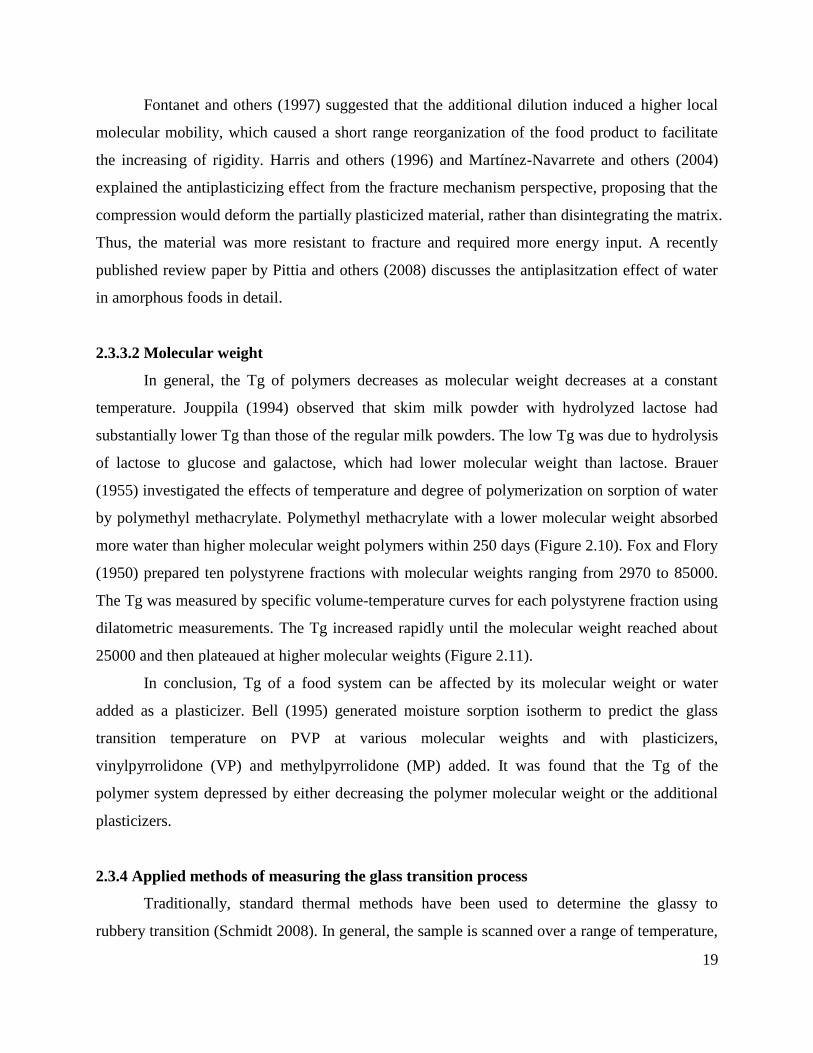
2.3.2 Critical water activity, moisture content, and the glass transition
Critical aw and moisture content can be considered as those depressing Tg to the
environmental temperature (Roos 1993). The BET monolayer value is always believed to be the
critical water content, below which dehydrated foods are most stable (Labuza 1970). However,
the critical moisture contents obtained by Roos (1993) differed significantly from the BET
monolayer values. Studies (Levine and Slade 1988; Roos and Karal 1991; Slade and Levine
1991) indicate that stickiness, collapse, and crystallization of amorphous materials occur at
temperatures above Tg. Thus, critical aw or moisture content (mc) at which the glass transition
occurs may be a better parameter to predict stability and storage conditions of amorphous
materials. A state diagram can be plotted, which reflects the relationship between Tg and
moisture content (or water activity) (Figure 2.6). For example, when Tg is equal to 25°C, the
critical aw and mc for maltodextrin (DE-4-7) are 0.7 and 11.2%, respectively. If the aw of
maltodextrin (M040) is higher than 0.7 at 25°C, Tg will be depressed to below the ambient
temperature, which affects chemical and physical stability of the material. The state diagram is a
valuable tool to manipulate both Tg and material behavior under various storage conditions
(Roos 1993). Roos (1994) also related milk powder stability to Tg and the corresponding critical
values for water content and aw in the state diagram.
Page 22
17
2.3.3 Factors that affect the glass transition
2.3.3.1 Water plasticization and antiplasticization
Water is the most important non-nutrient component, solvent, and plasticizer of food
solids, food components, and almost all biological materials (Roos 1995). Water is also one of
the lowest molecular weight plasticizers, with an extremely low Tg (Roos 1995). The molecular
weight of water is significantly lower than most food components, which lowers the local
viscosity and enhances molecular motion (Ferry 1980). Ferry (1980) also stated that water as a
diluent introduced additional free volume to the original system. Plasticization of food solids by
water is observed from the depression of the glass transition temperature with increasing water
content.
The glass transition process is the result of plasticization of food solids, which induces a
dramatic change in the mechanical properties of foods. Water can interact with the surface of
solids, which is known as adsorption, and water can penetrate the bulk solid structure, which is
known as absorption. There are two kinds of forces involved in adsorption: van der Waals
interactions and chemical adsorption by chemical bonding. Water molecules first adsorb onto the
surfaces of dry material to form a monolayer, which is subjected to both surface binding and
diffusional forces. As more water molecules adhere to the surfaces, diffusional forces exceed the
binding forces and moisture is transferred into the materials. When multilayer water forms, water
can be absorbed into the bulk structure by pores and capillary spaces (Barbosa-Canovas 1996).
The glass transition process occurs when water uptake changes from surface adsorption to bulk
absorption.
The efficiency of water as a plasticizer is based on the affinity of water for other
molecules and its ability to form a homogeneous mix without phase separation. Studies have
been done to investigate the consequences of water plasticization on a material’s mechanical
properties and relate the effect to the glass transition process. Roe (2005) studied the trehalose-
water system and concluded that the Tg value decreased more than 12°C as the moisture content
(%db) increased from 0% to 1%. Roos (1991) studied the effects of water, freeze-concentration
and effective molecular weight on Tg of maltose and maltodextrins using DSC. The Tg of the
sample at a specific moisture content was determined by a change in the heat capacity at the Tg
region using DSC. The decrease of Tg with increasing water content was substantial. The
Page 23
18
decrease of Tg was most significant as moisture content increased from 0 to 5 gH2O/100g dry
matter. Another study conducted by Ellis (1988) found that increasing the water content by 1%
for polyamides may induce a 15-20°C reduction in Tg while comparable concentrations of
organic diluents, such as amorphous Nylon blends, decrease the Tg only about 5 °C.
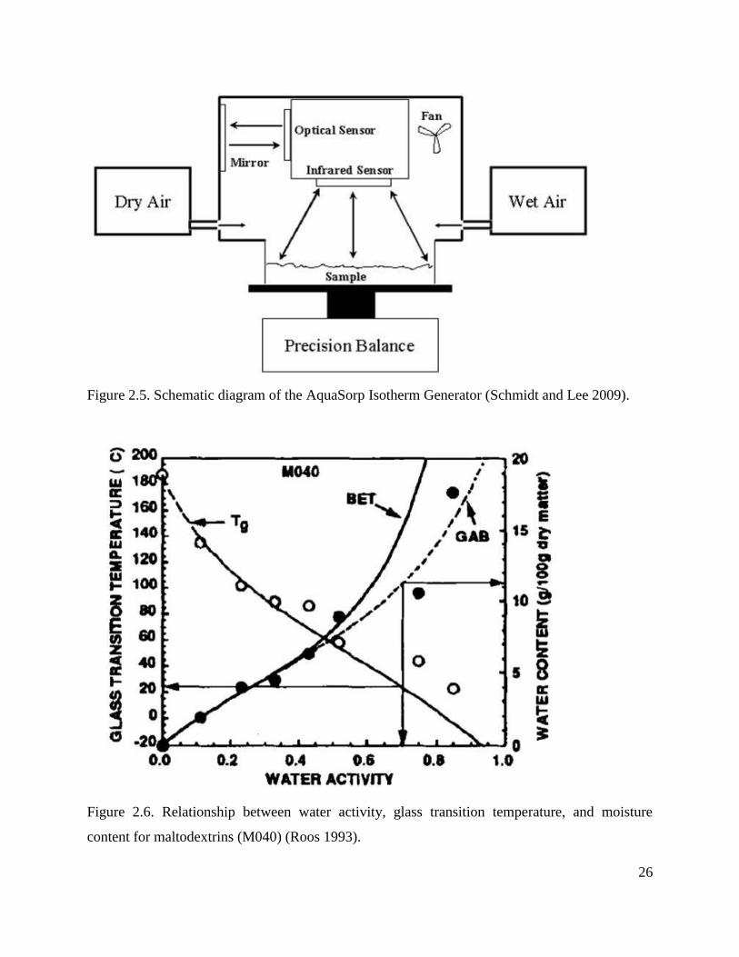
Oksanen and Zografi (1990) analyzed water vapor absorption isotherms of poly
(vinylpyrrolidone) at various temperatures along with the measurement of Tg as a function of
water content. They observed that the amount of water vapor absorbed at a particular relative
humidity increased with decreasing temperatures (Figure 2.7). They suggested that sufficient
water uptake (moisture content), which can be designated by the upward inflection of the
isotherm, was needed to be taken up to cause Tg to be less than the experimental temperature and
cause the polymer to transform into a rubbery state. At a higher temperature, less water is
required to plasticize the sample at the same water activity because of the higher molecular
mobility.
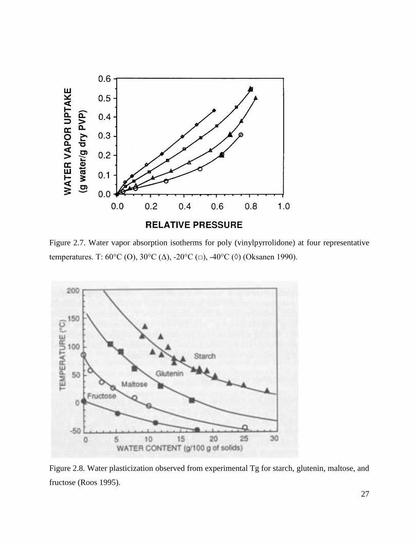
The effect of water on Tg of food components with various molecular weights is shown
in Figure 2.8 (Roos 1995). Starch and glutenin with relatively high molecular weights have
higher Tg at low moisture content than maltose and fructose with lower molecular weights. Since
the anhydrous Tg of fructose is fairly low and easy to depress below 0°C, the experimental
condition should be controlled when using low molecular weight carbohydrates with high
moisture content at room temperature.
However, water can exhibit an antiplasticizing effect. Instrumental and sensory
measurements have shown for many products that in a limited humidity range, where water
keeps its ability to decrease Tg, rigidity increases with increasing aw (Roudaut and others 1998;
Li and others 1998; Attenburrow and others 1992; Konopacka and others 2002; Spackman and
Schmidt 2009). Vrentas and others (1988) described this abnormal phenomenon as an
antiplasticizing effect: the addition of diluents, such as water, to the system delays the
movements of the polymer which is opposite to the one expected from a plasticization. For
example, the hardness of extruded bread was evaluated by sensory panelists and there was a
slight increase of stiffness intensity between 6% and 10% water (Roudaut and others 1998),
which suggests that the stiffening of the sample detected instrumentally is perceptible by the
consumer. Spackman and Schmidt (2009) also observed a significant increase in hardness
followed by a decrease at higher relative humidity in sugar gum pastes (Figure 2.9).
Page 24
19
Fontanet and others (1997) suggested that the additional dilution induced a higher local
molecular mobility, which caused a short range reorganization of the food product to facilitate
the increasing of rigidity. Harris and others (1996) and Martínez-Navarrete and others (2004)
explained the antiplasticizing effect from the fracture mechanism perspective, proposing that the
compression would deform the partially plasticized material, rather than disintegrating the matrix.
Thus, the material was more resistant to fracture and required more energy input. A recently
published review paper by Pittia and others (2008) discusses the antiplasitzation effect of water
in amorphous foods in detail.
2.3.3.2 Molecular weight
In general, the Tg of polymers decreases as molecular weight decreases at a constant
temperature. Jouppila (1994) observed that skim milk powder with hydrolyzed lactose had
substantially lower Tg than those of the regular milk powders. The low Tg was due to hydrolysis
of lactose to glucose and galactose, which had lower molecular weight than lactose. Brauer
(1955) investigated the effects of temperature and degree of polymerization on sorption of water
by polymethyl methacrylate. Polymethyl methacrylate with a lower molecular weight absorbed
more water than higher molecular weight polymers within 250 days (Figure 2.10). Fox and Flory
(1950) prepared ten polystyrene fractions with molecular weights ranging from 2970 to 85000.
The Tg was measured by specific volume-temperature curves for each polystyrene fraction using
dilatometric measurements. The Tg increased rapidly until the molecular weight reached about
25000 and then plateaued at higher molecular weights (Figure 2.11).
In conclusion, Tg of a food system can be affected by its molecular weight or water
added as a plasticizer. Bell (1995) generated moisture sorption isotherm to predict the glass
transition temperature on PVP at various molecular weights and with plasticizers,
vinylpyrrolidone (VP) and methylpyrrolidone (MP) added. It was found that the Tg of the
polymer system depressed by either decreasing the polymer molecular weight or the additional
plasticizers.
2.3.4 Applied methods of measuring the glass transition process
Traditionally, standard thermal methods have been used to determine the glassy to
rubbery transition (Schmidt 2008). In general, the sample is scanned over a range of temperature,
Page 25
20
while keeping the moisture content/water activity of the sample constant, resulting in the
determination of the glass transition temperature of the sample (Schmidt 2008). Currently, the
two most popular methods for determining the glass transition temperature are differential
scanning calorimetry (DSC) and mechanical spectroscopy (or dynamic mechanical thermal
analysis DMTA) (Le Meste and others 2002). These two techniques can produce significantly
different values based on different structural units, analysis methods, and definitions of Tg
(Kalichevsky and others 1992; Biliaderis and others 1999). DSC measures temperature of a
sample and a reference as a function of temperature. The phase transition causes the difference in
the energy supplied, which is recorded in a thermogram (Roos 1995). Applications of DSC in the
determination of phase transitions in foods include such changes as crystallization and melting of
water, lipids, and other food components, protein denaturation, and gelatinization and
retrogradation of starch. Samples are usually sealed in pans in order to maintain a constant water
content since water has an enormous effect on transition temperatures (Roos 1995).
Determination of glass transition temperature is challenging for food systems because of
their chemical and microstructural complexity (Le Meste and others 2002). DSC is often not
applicable for analyzing the Tg of complex food systems because of the possible occurrence of
multiple simultaneous thermal events, which might overlap with the glass transition. Since the
water sorption isotherm is already a vital requirement of food safety and quality assessment, it
would be highly desirable if a direct, practical means of determining the Tg from water vapor
sorption behavior of complex amorphous food materials could be established (Schmidt 2008).
Recently developed humidity generating instruments, such as the dynamic vapor sorption (DVS)
instrument, can determine the Tg from another angle, by keeping the temperature of the sample
constant but increasing/decreasing the sample aw. As a result, the glass transition process occurs
at a critical water activity (awc) or relative humidity (RHc) at a constant temperature. The RHc can
be extrapolated or calculated from the isotherm at a constant temperature. The corresponding
critical values for moisture content and aw at the glass transition temperature are showed in the
state diagram (Figure 2.12). Burnett and others (2004) developed a ramping method using the
DVS to determine the RHc values that induces the glass transition process at selected
temperatures. The glass transition RHc was measured at the intersection between surface
adsorption and absorption into the bulk structure (Figure 2.13). The results obtained from the
DVS ramping experiments were compared to values obtained from IGC experiment. The
Page 26
21
discrepancies may be understood by the following factors (Burnett and others 2004): 1) the
sample water activity cannot catch up with the change of relative humidity in DVS, especially
with a higher ramping rate, which leads to higher glass transition values, 2) IGC experiments
were done at defined, equilibrated temperatures while the DVS values used a temperature ramp
and any slight humidity change might alter the Tg by several degrees, 3) comparison depends on
the definition of Tg in the DSC curve: onset, midpoint, and endpoint.
2.4 Mechanical Properties
Mechanical properties of foods are important to their behavior in processing, storage,
distribution, and consumption. The physical state of food solids is one of the most important
factors that affect the mechanical properties of low-moisture and frozen foods in which small
changes in temperature or water content may significantly affect the physical state due to the
phase transition (Roos 1995). Thus, appropriate equipment should be selected to evaluate the
tolerance of mechanical stress during manufacturing, storage, and consumption.
Stiffness can be used as a general term to refer to the response of food materials to an
external stress. Changes in stiffness occur over the glass transition process, which describes the
changes in mechanical properties as a function of temperature, moisture content or water activity.
The stiffness-temperature-moisture relationship of biomaterials around their glass transition can
be related and analyzed using mathematical models (Peleg 1993). Figure 2.14 shows the stiffness
versus temperature relationship of an amorphous glucose glass as well as the stiffness versus
moisture relationship of wheat grains when fitting to an empirical model. These models
demonstrated that water at a constant temperature has an effect on mechanical properties similar
to that caused by an increase in temperature at constant water content. Water content or
temperature had a significant effect on stiffness, which decreased with increasing water content
or temperature, especially at or around the glass transition region (Peleg 1993).
As temperature or aw of the food materials changes, the mechanical properties will be
reflected by the textural changes of breakfast cereals, the tendency of powders to agglomerate,
and even the viability of microbial spores (Peleg 1993). Furthermore, mechanical properties of
amorphous foods, such as food powders and cereal foods, are very important in defining various
quality parameters, including flowability properties, stickiness, and stiffness. Modeling the
mechanical properties or stiffness as a function of temperature and water content provides a
Page 27
22
valuable tool for estimating changes, which may occur during exposure to abusing
environmental conditions (Roos 1995). Various studies have investigated the crispiness of low-
moisture foods and related mechanical properties to their water content and temperature. Some
common approaches involved both instrumental and sensory analysis (Rouduat and Le Meste
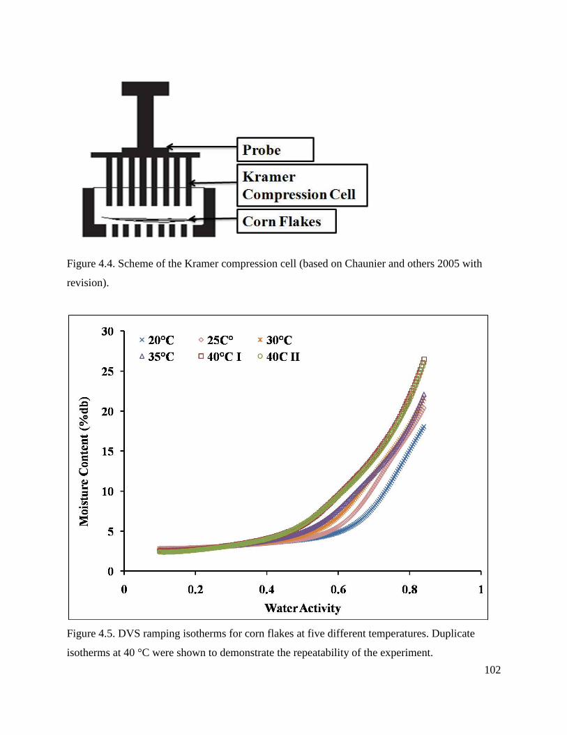
1998; Suwonsichon and Peleg 1998; Chaunier and others 2005; Chaunier and others 2007).
Rouduat and Le Meste (1998) studied the texture properties of crispy breads using compression
test, acoustic measurements and sensory analysis. They proposed that the effect of water
plasticization on brittle character, on crispness by sensory test, and on intensity of the sound
emitted at fracture by acoustic measurements were due to the onset of molecular motions
preceding and accompanying the glass transition. Sauvageot and Blond (1991) also studied the
crispness of three breakfast cereals by sensory and mechanical analysis. Crispness was plotted
against aw and the critical water activity values were obtained. They found a good correlation
between the results of the sensory methods and instrumental penetration test corresponding to the
critical water activity value. However, the research did not clarify the reasons for the dramatic
decrease crispness within a fairly narrow water activity range, which might be explained by the
occurrence of the glass transition.
It should be noted that both instrumental textural and sensory tests only investigate the
crunchiness, crispness, and hardness of the material on the macroscopic level. The stability and
quality of amorphous food powders, such as polydextrose, can also be greatly affected by the
fluctuation of temperature and water content. However, the hardness and viscosity of food
powders are difficult to determine by sensory tests and direct textural analysis. Thus, probing
from another angle, we proposed to investigate the mechanical properties of food powders from
the microscopic level, such as force measurements using atomic force microscopy (AFM) (Butt
and others 2005). An examination of force curves can prove useful in determining adhesion and
hardness characteristics of samples. The examples in Figure 2.15 represent some of the general
variations in force curves. Price and others (2002) used the AFM probe technique to investigate
the effect of relative humidity on the adhesion properties of pharmaceutical powder surfaces. The
results showed that the adhesion interactions increased significantly with each incremental rise in
humidity. Hooton and others (2004) further observed that the particle adhesion as a function of
humidity is highly affected by surface chemistry and asperity geometry difference by using the
AFM technique.
Page 28
23
Thus, investigating the mechanical properties of low-moisture amorphous food materials
would be useful for estimating the physical state and phase transitions, especially incorporated
with the analysis of the sorption behavior of the food.
2.5 Figures and tables
Figure 2.1. Generalized moisture sorption isotherm divided into three regions based on water
properties (Fennema 1996).
Page 29
24
Figure 2.2. The IUPAC classification for adsorption isotherms (from Donohue, 2004)
Figure 2.3. Weight average isotherms are used for multicomponent food systems (from Labuza,
1984.).
Page 30
25
Figure 2.4. Schematic diagram of the DVS Intrinsic (from DVS Intrinsic Operation Manual,
Version 1.0, SMS).
Page 31
26
Figure 2.5. Schematic diagram of the AquaSorp Isotherm Generator (Schmidt and Lee 2009).
Figure 2.6. Relationship between water activity, glass transition temperature, and moisture
content for maltodextrins (M040) (Roos 1993).
Page 32
27
Figure 2.7. Water vapor absorption isotherms for poly (vinylpyrrolidone) at four representative
temperatures. T: 60°C (O), 30°C (Δ), -20°C (□), -40°C (◊) (Oksanen 1990).
Figure 2.8. Water plasticization observed from experimental Tg for starch, glutenin, maltose, and
fructose (Roos 1995).
Page 33
28
Figure 2.9. DVS and DDI water vapor sorption isotherms and effect of increasing %RH on the
hardness of the four gum paste materials stored at 25°C (Spackman and Schmidt 2009).
Figure 2.10. Effect of molecular weight on sorption and desorption of water by polymethyl
methacrylate (Brauer 1955).
Page 34
29
Figure 2.11. Tg of polystyrene fractions vs. molecular weight (upper curve) and vs. M-1
(lower
curve) (Fox and Flory 1950).
Figure 2.12. The effect of temperature and %moisture content or aw on the glassy to rubbery
transition process (Schmidt 2008).
Page 35
30
Figure 2.13. Relative humidity ramping experiment (6.0% RH/hr) for spray-dried lactose sample
at 25°C. Solid line shows the net change in mass while the dotted line shows the RH profile
(Burnett 2004).
Figure 2.14. Stiffness versus temperature and moisture content relationships of amorphous
glucose and wheat grains (Peleg 1993).
Page 36
31
Figure 2.15. General examples of force curves from AFM (Basic SPM Training Course).
Table 2.1. Specifications of the AquaSorp Isotherm Generator.
Page 37
32
Table 2.2. Salt solution aw values used for AquaSorp calibration obtained from Decagon Devices
(Pullman, WA).
2.6 References
Ahlneck C, Zografi G. 1990. Molecular basis of moisture effects on the physical and chemical
stability of drugs in the solid state. International Journal of Pharmaceutics. 62: 87-95.
Alam A, Shove GC. 1973. Hygroscopicity and thermal properties of soybeans. Transactions of
the American Society of Agrigultural Engineers. 16: 707-709.
Attenburrow GE, Davies AP, Goodband RM, Ingman SJ. 1992. The fracture behavior of starch
and gluten in the glassy state. J Cereal Sci. 16:1-12.
Barbosa-Cánovas GV, Vega-Mercado H. 1996. Physical, chemical, and microbiological
characteristics of dehydrated foods. International Thompson Publishing, New York, USA, pgs,
29-99.
Barbosa-Canovas GV, Fontana AJ, Schmidt SJ, Labuza TP. 2007 Water activity in foods.
Blackwell Publishing Professional, Iowa, USA.
Basic SPM training course. 2000. Digital Instruments Veeco, Inc. Available from AFM training
sessions offered by materials research laboratory, University of Illinois at Urbana-Champaign.
Biliaderis CG, Lazaridou A, Arvanitoyannis I. 1999. Glass transition and physical properties of
polyol-plasticized pullulan-starch blends at low moisture. Carbohydrate Polymers. 40:29-47.
Page 38
33
Brauer GM, Sweeney WT. 1955. Sorption of water by polymethyl methacrylate. Modern Plastics
32(9):138.
Brunauer S, Deming LS, Deming WE, Teller E. 1940. On a theory of the van der Waals
adsorption of gases. Journal of the American Chemical Society 62(7):1723-6.
Burnett DJ, Thielmann F, Booth J. 2004. Determining the critical relative humidity for moisture-
induced phase transitions. International Journal of Pharmaceutics (287):123-33.
Butt JH, Cappella B, Kappl M. 2005. Force measurements with the atomic force microscope:
technique, interpretation and applications. Surface Science Reports. 59: 1-152.
Byrn S. 1982. Solid State Chemistry of Drugs. Academic Press, New York. pp: 7-10.
Chang YP, Cheah PB, Seow CC. 2000. Plasticizing-antiplasticizing effect of water on tapioca
starch films in the glassy state. J Food Sci. 65(3):445-451.
Chaunier L, Courcoux P, Valle GD, Lourdin D. 2005 Physical and sensory evaluation of
cornflakes crispness. Journal of Texture Studies. 36: 93-118.
Chaunier L, Valle GD, Lourdin D.2007 Relationships between texture, mechanical properties
and structure of cornflakes. Food Research International. 40: 493-503.
Chen T, Flower A, Toner M. 2000. Literature review: supplemented phase diagram of the
trehalose-water binary mixture. Cryobiology. 40: 277-282.
Christen GL. 2000. A rapid method to determine the sorption isotherms of peanuts. J. Agric. Eng.
Res. 75:401-408.
Decagon Devices. 2007. AquaSorp Operator's Manual. 2nd ed. Pullman, WA: Deagon Devices,
Inc.
Donohue, M. 2004 New classification of adsorption isotherms.
http://www.nigelworks.com/mdd/PDFs/NewClass.pdf (Accessed at Jan 9, 2010).
Page 39
34
Ellis TS. 1988. Moisture-induced plasticization of amorphous polyamides and their blends.
Journal of Applied Polymer Science. 36: 451-466.
Franks F. 1991. Water activity: a credible measure of food safety and quality. Trends Food Sci.
Technol. 2:68–72.
Fellows, J. 2000. Food processing technology. Woodhead Publishing Limited, Cambridge,
England.
Fennema OR. 1996. Food Chemistry. Marcel Dekker, Inc., New York, USA
Ferry JD. 1980. Viscoelastic Properties of Polymers. 3nd ed. John Wiley& Sons, New York.
Fontanet I, Davidou S, Dacremont C, Le Meste M. 1997. Effect of water on the mechanical
behavior of extruded flat bread. J Cereal Sci. 25:303-311.
Fox TG, And Flory PJ. 1950. Second-order transition temperatures and related properties of
polystyrene. I. influence of molecular weight. Journal of Applied Physics. 21: 581-591.
Harris M, Peleg M. 1996. Patterns of textural changes in brittle cellular foods caused by moisture
sorption. Cereal Chem. 73: 225-231.
Hooton JC, German CS, Allen S, Davies MC, Roberts CJ, Tendler SJB, Williams PM. 2004. An
atomic force microscopy study of the effect of nanoscale contact geometry and surface chemistry
on the adhesion of pharmaceutical particles. Pharmaceutical Research. 21(6): 953-961.
Jouppila K, Roos YH. 1994. Glassy transitions and crystallization in milk powders. Journal of
Dairy Science (77):2907-15.
Kalichevsky MT, Jaroskiewicz EM, Ablett S, Blanshard JMV, Lillford PJ. 1992. The glass
transition of amylopectin measured by DSC, DMTA and NMR. Carbohydrate Polymers. 18:77-
88.
Page 40
35
Karel, M. 1975. Physicao-chemical modifications of the state of water in foods: A speculative
survey. In: Water Relations of Foods, Duckworth, RB. London: Academic Press.
Konopacka D, Plocharsky W, Beveridge T. 2002. Water sorption and crispness of fat-free apple
chips. J Food Sci. 67(1):87-92.
Kontny MJ, Zografi G. 1995. Sorption of water by solids. Marcel Dekker Inc., New York, pgs,
387-418.
Labuza, TP. 1968. Sorption phenomena in food. Food Technology. 22(3):15.
Labuza TP, Tannenbaum SR, Karel M. 1970. Water content and stability of low-moisture and
intermediate moisture foods. Food Technology. 24(5): 543-550.
Le Meste M, Champion D, Roudaut G, Simatos D. 2002. Glass transition and food technology:
A critical appraisal. Journal of Food Science. 67:2444-2458.
Levine H, Slade L. 1986. A polymer physical-chemical approach to the study of commercial
starch hydrolysis products (SHPs). Carbohydrates and Polymers. 6:213-244.
Levine H, Slade L. 1988. Water as a plasticizer: Physico-chemical aspects of low-moisture
polymer systems. In: F. Franks, editor. Water Science Reviews 3: Water Dynamics. Cambridge,
UK: Cambridge University Press. p 79-185.
Levoguer CL, Williams DR. 1997. The characterization of pharmaceutical materials by dynamic
vapor sorption. London: Surface Management Systems. Application Note 101. Available from
SMS, London, UK.
Lewis GN. 1907. Outlines of a new system of thermodynamic chemistry. Proceedings of the
American Academy of Arts and Sciences, 43(7): 259-293.
Lewis GN, Randall M. 1923. Thermodynamics and the Free Energy of Chemical Substances.
McGraw-Hill, New York.
Page 41
36
Li Y, Kloeppel KM, Hsieh F. 1998. Texture of glassy corn cakes as function of moisture content.
J Food Sci. 63(5):869-872.
Lillie MA. 1990. The effects of hydration on the dynamic mechanical properties of elastin.
Biopolymers 29(8-9):1147.
Martínez-Navarrete N, Moraga G, Talens P, Chiralt A. 2004. Water sorption and the
plasticization effect in wafers. International Journal of Food Science and Technology. 39(5):
555–562.
McBai JW. 1935. An explanation of hysteresis in the hydration –dehydration of gels. Journal of
the American Chmical Society. 57: 699.
Oksanen CA, Zografi G. 1990. The relationship between the glassy transition temperature and
water vapor absorption by poly(vinylpyrrolidone). Pharmaceutical Research 7(6):654-7.
Peleg M. 1994. A model of mechanical changes in biomaterials at and around their glass
transition. Biotechnol Prog 10(4):385.
Peleg M. 1993. Mapping the stiffness-temperature-moisture relationship of solid biomaterials at
and around their glass transition. Rheologica acta 32(6):575.
Pittia P, Sacchetti G. 2008. Antiplasitzation effect of water in amorphous foods: A review. Food
Chemistry. 106: 1417–1427.
Price R, Young PM. Edge S. Staniforth JN. 2002. The influence of relative humidity on
particulate interactions in carrier-based dry powder inhaler formulations. International Journal of
Pharmaceutics. 246: 47-59.
Rahman MS. 2009. Food properties handbook. Boca Raton, FL: CRC Press.
Rao SK, Das B. 1968. Varietal differences in gelatin, egg albumin, and casein in relation to
adsorption-desorption hysteresis with water. Journal of Physical Chmistry. 72: 1233.
Page 42
37
Roe KD, Labuza TP. 2005. Glass Transition and crystallization of amorphous trehalose-sucrose
mixtures. International Journal of Food Properties. 8: 559-574.
Roos Y, Karel M. 1991. Plasticizing effect of water on thermal behavior and crystallization of
amorphous food models. J. Food Sci. 56: 38.
Roos YH. 1993. Water activity and physical state effects on amorphous food stability. Journal of
Food Processing and Preservation 16(6):433-47.
Roos YH. 1995. Phase transitions in foods. San Diego, CA: Academic Press, Inc.
Roudaut G, Dacremont C, Le Meste M. 1998. Influence of water on the crispness of cereal based
foods: acoustic, mechanical, and sensory studies. J Texture Stud. 29:199-213.
Sauvageot F, Blond G. 1991. Effect of water activity on crispness of breakfast cereals. Journal of
Texture Study. 22: 423-442.
Schmidt SJ. 2004. Water and solids mobility in foods. Advances in Food and Nutrition Research,
Academic Press, London, UK, vol. 48, pgs, 1-101.
Schmidt SJ. 2008. Determining the critical water activity at which the glassy to rubbery
transition occurs in amorphous food materials using recently developed dynamic water sorption
technology. Midwest Advanced Food Manufacturing Alliance (MAFMA) Grants
Scott WJ. 1957. Water relations of food spoilage organisms. Advances in Food Research 7:83-
127.
Sing KSW, Haul RAW, Pierotti RA, Siemieniewska T. 1985. Reporting physisorption data for
gas/solid systems with special reference to the determination of surface area and porosity. Pure
& Appl. Chem. 57(4): 603-619.
Slade L, Levine H. 1991. Beyond water activity: Recent advances based on an alternative
approach to the assessment of food quality and safety. Critical Reviews in Food Science and
Nutrition. 30: 115-360.
Page 43
38
Spackman CW, Schmidt SJ. 2009. Characterizing the physical state and textural stability o sugar
gum pastes. Food Chemistry. 119 (2): 490-499.
Sperling LH. 1986. Introduction to Physical Polymer Science. Wiley, New York.
Surface Measurement Systems online [Internet]. London, UK: SMS 2008 [Accessed 2010 Mar
17]. Available from: http://www.thesorptionsolution.com/Products_DVS_Intrinsic.php.
Suwonsichon T, Peleg M. 1998. Instrumental and sensory detection of simultaneous brittleness
loss and moisture toughening in three puffed cereals. Journal of Texture Studies. 29: 255-274.
Thiel PA, Madey TE. 1983. The interaction of water with solid surfaces: fundamental aspects.
Surface Sci. Rep. &: 1381-1388.
Troy HC, Sharp PF. 1930. α and β lactose in some milk products. Journal of Dairy Science. 12:
140.
Van Campen L, Amidon GL, Zografi G. 1983. Moisture sorption kinetics for water-soluble
substances: theoretical considerations of heat transport control. Journal of Pharmaceutical
Sciences 72(12): 1381-8.
Vrentas JS, Duda JL, Ling H. 1988. Antiplasticization and volumetric behavior in glassy
polymers. Macromol. 21:1470-1475.
White GW, Cakebread SH. 1966. The glassy sate in certain sugar-containing food products.
Journal of Food Technology. 1:73-81.
Yu X. 2007a. Investigation of moisture sorption properties of food materials using saturated salt
solution and humidity generating techniques. [dissertation]. Urbana, IL: University of Illinois at
Urbana-Champaign.
Yu X, Kappes SM, Bello-Perez LA, Schmidt SJ. 2007b. Investigating the moisture sorption
behavior of amorphous sucrose using a dynamic humidity generating instrument. Journal of
Food Science. 73 (1): 25-35.
Page 44
39
CHAPTER 3.DETERMINATION OF THE CRITICAL RELATIVE HUMIDITY (RHc)
FOR POLYDEXTROSE USING A HUMIDITY GENERATING INSTRUMENT
3.1 Abstract
The rubbery to glassy transition in amorphous materials can be described either by a glass
transition temperature (Tg) at a specified moisture content or a critical relative humidity (RHc) at
a specified temperature. Newly developed automated sorption isotherm instruments have the
advantages of high data resolution capacity and short experimental times compared to the
traditional saturated salt slurry method. Studies have shown the ability of automated sorption
isotherm instruments to detect the glassy to rubbery transition (Burnett 2004; Yuan 2009).
However, there was no research using a dynamic vapor sorption (DVS) instrument using
different methods at various temperatures compared to the traditional method for the purpose of
investigating the glassy to rubbery transition. The objectives of this research were to: 1)
determine the RHc for amorphous polydextrose at various temperatures using the DVS ramping
and equilibrium methods and the conventional isotherm method, and 2) compare the RHc results
to the Tg values obtained via differential scanning calorimetry (DSC). The automated adsorption
isotherms were obtained from 20 to 40°C at 5°C intervals using the DVS. The DVS ramping
isotherm was obtained at a linearly increasing relative humidity (RH), 2%RH/hr, from 10 to
85%RH. The DVS equilibrium isotherm was obtained at twelve RH values using a dm/dt
criterion of 0.0005%. The conventional saturated salt slurry isotherm was obtained at 25°C using
ten saturated salt slurries, with RH values ranging from 11.3 to 84.3%. The RHc was identified
as the %RH that exhibited the fastest change in slope determined by the maximum in the second
derivative of the isotherm curve. The RHc and temperature values were plotted in a state diagram
and compared to DSC Tg values obtained at ten RH values from 11.3% to 84.3%. As predicted
from theory, RHc values decreased as temperature increased. As plotted on the state diagram,
RHc values were similar to the DSC Tg values. At the same temperature, the RHc order for the
isotherms was conventional < DVS equilibrium < DVS ramping, with the RHc values depending
on the time the material was exposed to the different RH conditions. This research showed that
the DVS instrument to be useful for routine determination of the glassy to rubbery transition in
amorphous food materials.
Page 45
40
3.2 Introduction
The introduction of the food polymer science (FPS) approach to study food ingredients
and systems, pioneered by Slade and Levine (e.g., 1987 and 1991), has revolutionized the topic
of moisture management in food systems and has been the impetus for numerous research studies
exploring the FPS approach for the assessment of food quality, stability, and safety (e.g., Roos
and Karel 1991; Roe and Labuza 2005). One of the key elements of the FPS approach is the
glass transition and its relationship to the processibility, product properties, quality, stability, and
safety of food systems. The glass transition can be defined as a transformation of a supercooled
liquid (rubbery state) to a highly viscous (>1012
Pa·s), solid-like glass (Barbosa-Canovas and
Others 2007). When the material transforms from the rubbery to the glassy state, the molecules
become mobile, gaining rotational and translational mobility (Barbosa-Canovas and others 2007).
Therefore, the glass transition can alter food structure and microstructure, crystallization, rates of
diffusion, stabilization of microbial cells and spores, and chemical and biochemical reactions
(Roos 1995; Chirife and Buera 1996; Le Meste and others 2002).
Traditionally, thermal methods, such as differential scanning calorimetry (DSC), are used
to determine the glassy to rubbery transition, where the sample is scanned over a range of
temperatures, while keeping the moisture content constant, resulting in the determination of the
Tg of the sample. Determination of the Tg using a thermal method is especially challenging for
food ingredients and systems because of their chemical and microstructural complexity (Le
Meste and others 2002). Two major disadvantages of using DSC for measuring Tg are: 1) low
sensitivity and 2) possible occurrence of multiple thermal events (e.g., starch gelatinization,
protein denaturation) that may overlap or interfere with the glass transition.
Besides standard thermal methods, the glass transition process can also be detected by
changing the relative humidity at a constant temperature. Since the water sorption isotherm is
already a vital requirement of food safety and quality assurance, it would be highly desirable if a
direct, practical means of determining the Tg from water vapor sorption behavior of complex
amorphous food materials could be established (Schmidt 2008). Oksanen and Zografi (1990)
analyzed water vapor absorption isotherms of poly (vinylpyrrolidone) using the saturated salt
slurry method at various temperatures along with the measurement of Tg as a function of water
content by DSC. They suggested that sufficient water uptake (moisture content), which was
Page 46
41
located in the upward inflection of the isotherm, was considered to cause Tg to be less than the
experimental temperature and cause the polymer to transition into the rubbery state.
The saturated salt slurry method can be used to generate isotherms, in which the upward
curve indicates the glassy to rubbery transition at a constant temperature. The saturated salt
slurry method has the advantage of generating accurate water activity values by providing the
sample the opportunity to reach its equilibrium moisture content due to relatively long
experimental times. However, Levoguer (1997) summarized four major disadvantages of using
the saturated salt slurry method: 1) the long period of time it takes the product to achieve
equilibrium, 2) the difficulty of obtaining accurate measurements due to exposure of the sample
to an environment which often has a different relative humidity, 3) the requirement of using large
sample sizes to obtain a measurement, and 4) the time-consuming and labor intensive nature of
the method. In addition to these disadvantages summarized by Levoguer (1997), the saturated
salt slurry method only generates a limited number of data points, which obstructs the precise
detection of the upward curve induced by the glass transition process.
In order to overcome the disadvantages of the saturated salt slurry method, recently
developed humidity generating instruments, such as the dynamic vapor sorption (DVS)
instrument and the AquaSorp humidity generator, can determine the Tg, by keeping the
temperature of the sample constant while increasing the sample water activity (or relative
humidity), similar to the saturated salt slurry method but with nearly continuous data point
collection. As a result, the glass transition process occurs at a critical water activity (awc) or
relative humidity (RHc) at a constant temperature. The RHc can be extrapolated or calculated
from the isotherm at a constant temperature. Thus, the RHc values can be obtained from the
isotherm as a function of temperature, similar to Tg values being obtained as a function of
moisture content (or water activity) using a thermal method. The corresponding critical values
for moisture content and aw at the glass transition temperature are shown in the state diagram
(Figure 3.1). Burnett and others (2004) developed a ramping method using the DVS to determine
the RHc value, which induces the glass transition process at specific temperatures. For spray-
dried lactose, at low RH values (below 30% RH), water uptake was relatively low and moisture
uptake in this region was dominated by surface adsorption. Above 40% RH there was a sharp
increase in moisture sorption, most likely due to bulk absorption dominating the sorption process.
The RHc that induces the glass transition at the experimental temperature was measured as the
Page 47
42
extrapolated intersection between surface adsorption of water vapor and absorption of water
vapor into the bulk structure. The results obtained from DVS ramping experiments were
compared to Tg values obtained from IGC and the literature DSC experiments. Burnett and
others (2004) concluded that considering the different approaches and the uncertainties in
measuring the Tg by three methods, the small differences in the DVS, DSC, and IGC values are
not surprising. The DVS values represent the onset of the glassy to rubbery transition and the
IGC values represented the middle of the glassy to rubbery transition.
Yuan (2009) investigated the relationship between the glassy to rubbery transition using
thermal methods, such as DSC and modulated differential scanning calorimetry (MDSC) and the
AquaSorp humidity generating instrument and concluded that RHc values obtained from the
AquaSorp instrument were indicative of the glassy to rubbery transition. However, none of these
studies investigated the difference between the automated isotherm RHc and the conventional
saturated salt slurry RHc, which allows the sample to reach steady-state equilibrium.
Polydextrose was chosen as a model material for this research because it does not
participate in moisture induced recrystallization (Ribeiro and others 2003). It is a non-crystalline
material due to the highly branched, random bonds of α and β linkages resulted from the thermal
polymerization of D-glucose (Tale and Lyle 2006). The polydextrose used in this study has a
minimum purity of 90%. Other components include dextrose (4% max), sorbitol (2% max) and
levoglucosan (4% max) (Tale and Lyle 2006). Sorbitol and citric acid can be present as a
plasticizer and catalyst in the polymerization reaction.
Polydextrose is a multifunctional food ingredient that can be used as a humectant,
texturizer, thickener, stabilizer, and cryoprotectant (Mitchell 1996). For example, solutions of
polydextrose have a higher viscosity than sucrose or sorbitol solutions at equivalent
concentrations and temperatures, which enables polydextrose to provide the desirable mouth feel
and textural qualities when replacing sugars and fats. It is odorless and has no sweetness and an
energy value of only 1 Kcal/g (Mitchell 1996). Since polydextrose is not sweet, it may be used in
savory applications as a humectant to control the water activity of a product and hence help to
increase shelf life (Mitchell 1996). Unlike the polyols, polydextrose takes part in the Maillard
reaction with amino acids, similar to reducing sugars, allowing the characteristic flavors of
caramel and toffee to develop (Mitchell 1996).
Page 48
43
Polydextrose was used to validate the hypothesis that newly developed automated
sorption isotherm methods, including ramping and equilibrium isotherms, using DVS, coupled
with the saturated salt slurry method, were associated with the glassy to rubbery transition
obtained by DSC where samples were pre-equilibrated to different relative humidity values. The
specific objectives of this study were to 1) determine the RHc for amorphous polydextrose at
various temperatures using the DVS ramping and equilibrium methods and the traditional
isotherm method, and 2) compare the RHc results to the Tg values obtained via differential
scanning calorimetry (DSC).
3.3 Materials and Methods
3.3.1 Materials
Polydextrose (STA-LITE® III) was provided by Tate & Lyle (Decatur, IL). The
physicochemical properties of the polydextrose used in this study are summarized in Table 3.1.
The sample was sealed in its original container using parafilm in between each use and stored
under room conditions. Polydextrose moisture contents via vacuum oven drying at 30 in Hg and
60°C for 24 hours, and aw values, via an AquaLab Series 4 aw meter (Decagon Devices Inc.,
Pullman, WA) were measured throughout the duration of the study. The average moisture
content was 4.48% ± 0.09% (%wb) and the average aw value was 0.286±0.036. The slight
variation in these values were attributed to fluctuations in the ambient relative humidity.
3.3.2 Critical relative humidity determined using DVS
3.3.2.1 DVS calibration, probe check, and sample
A Dynamic Vapor Sorption (DVS) Intrinsic system (Surface Measurement System,
London, UK) was used to obtain isotherms from 20 to 40°C at 5°C intervals. The DVS
instrument was calibrated using three saturated salt slurries: LiCl, MgCl2, and NaCl at each
temperature every 6 months. The calibration was based upon the principle that the vapor pressure
above a saturated salt slurry in equilibrium with its surroundings should be constant at a
particular temperature. The salt solution %RH values, as a function of temperature, are listed in
Table 3.2.
Page 49
44
A relative humidity probe check was done before each run if the temperature was
changed in order to verify the relative humidity sensor and temperature probe performance. The
probe check aligned the probe sensor %RH with the target %RH. The procedure was done at ten
relative humidity values ranging from 10 to 90% at 10% RH intervals and at 95%, with a stage
time of 30 minutes each.
The DVS sample pan was cleaned before use by first rinsing with distilled water and then
ethanol. The pan was dried in a dust-free environment. A polonium strip was placed in the DVS
chamber to remove static electricity.
3.3.2.2 Ramping sorption isotherm determined using DVS
A 13 mm quartz round-bottom pan (50 mg) was used for all experiments. The sample pan
was removed from the microbalance to pre-weigh the sample (approximately 10 mg) on an
analytical balance to prevent overloading the balance. The sample was place in the DVS at a
constant temperature where it was initially dried in a 200 sccm (standard cubic centimeters)
stream of 10%RH nitrogen gas for 400 min in order to establish an initial sample equilibrium aw
value of 0.10. The sample was then exposed to a linearly increasing relative humidity from 10%
RH to 85% RH using a ramping rate of 2%RH/h. The same experiment was performed at 20°C,
25°C, 30°C, 35°C, and 40°C.
Weight change was converted to moisture content (%db) by calculating the amount of
water in grams in the initial sample and adding or subtracting (relative humidity dependant)
moisture based on the weight change measured by the DVS. The total amount of water in grams
was then divided by the grams of polydextrose in the initial sample to calculate the moisture
content on a % dry basis. Since each DVS ramping experiment yields a unique set of isotherm
values, the data points cannot be averaged. For clarity, only one isotherm was plotted at each
temperature for the DVS ramping method, except duplicate isotherms were shown at 40 °C to
demonstrate the repeatability of the experiment. The RHc values were obtained by three analysis
methods: the linear extrapolation method, the optimized MATLAB second derivative algorithm
developed by Yuan (2009), and the Savitzky-Golay method, a least square method (Savitzky and
Golay 1964).
Sorption isotherms often exhibit a critical turning point where the isotherm curve deviates
from the initial flat region and begins to take up more water, where water uptake changes from
Page 50
45
surface adsorption to bulk absorption. Traditionally, the turning point was determined by fitting
two straight lines before and after the critical points and determining their intersection point
(Burnett and others 2004). However, the selection of the data points for generating the straight
line is often arbitrary, which increases the uncertainty of the analysis.
In calculus, the second derivative is the derivative of the derivative of a function.
Generally speaking, the second derivative measures how the rate of the change of a quantity is
changing. Thus, the maximum of the second derivative exhibits the largest change in slope,
which was selected to represent the RHc. Both the MATLAB (The MathWorks, Inc., U.S.,
Version 7.6.0.324) second derivative algorithm and the Savitzky-Golay method use the concept
of the second derivative in order to determine the RHc value. The Savitzky-Golay method
smoothes the derivatives by a least-squared technique. A polynomial is fitted through a data
interval of (2m+1) points and a value is calculated as the middle interval. This procedure is
repeated until the entire data set has been smoothed. However, the Savitzky-Golay method was
only developed for equally spaced data points and is thus not applicable for cases having
unequally spaced data.
The MATLAB second derivative method was developed by Yuan (2009) and was
utilized to determine the RHc of each isotherm. The smoothing spline method was chosen for the
MATLAB second derivative algorithm. According to Yuan (2009), the first derivative was
calculated and then fitted by the smoothing spline function. The derivative of the fitting of the
first derivative was then calculated at locations every 0.001 unit apart of the total range, which
resulted in an overall second derivative of the original isotherm data with a resolution of
0.001.The maximum of the second derivative value was determined as the RHc value of the
isotherm.
The RHc values from the DVS ramping experiment obtained by these three methods
were analyzed using a complete randomized design at five temperatures using SAS (Statistical
Analysis System, Version 9.2). LSD (least significant difference) was used as a criterion to
differentiate these three methods at each temperature.
3.3.2.3 Equilibrium sorption isotherm determined using DVS
The polydextrose sample (~10mg) was measured into the quartz pan. The experiment
was done at 20°C, 25°C, 30°C, 35°C, and 40°C. Samples were first exposed to 10% relative
Page 51
46
humidity nitrogen gas flow (200 sccm) for 400 min to establish an initial sample equilibrium aw
value of 0.10, followed by exposure to twelve target relative humidity values selected to cover
the entire water activity range of the isotherm. Some of the target relative humidity values were
selected to be the same as the relative humidity values that could be generated by the saturated
salt slurries for comparison purposes. These ten salt slurries are listed in Table 3.3. The twelve
target relative humidity values were 11.3%, 22.5%, 32.8%, 38.0%, 43.2%, 48.0%, 53.0%, 57.6%,
63.0%, 68.9%, 75.3% and 84.3%. A dm/dt criterion of 0.0005% with a minimum stage time of
10 minutes and maximum wait time of 2000 minutes were utilized. Experiments were done in
duplicate. Dry nitrogen flow was set at 200 sccm (standard cubic centimeter per minute) during
the experiments. The data were exported to the DVS Standard Analysis Suite v6.0, which was
embedded in the Add-In function in Microsoft Excel. The last ten data points at each stage were
averaged and used to calculate the moisture content (db%) at each relative humidity, using the
initial moisture content previously determined by the vacuum oven drying method. The RHc of
each isotherm was obtained using the MATLAB second derivative method (Figure 3.2). The
linear extrapolation and the Savitzky-Golay methods were not applicable because of the limited
number of experimental data points.
3.3.3 Critical relative humidity determined using saturated salt slurry method
In order to cover the entire %RH range, 10 salts were chosen to obtain the equilibrium
isotherm at 25°C (Table 3.3). Saturated salt slurries were made by adding an excess amount of
salt into deionized water. The slurry was heated (~50°C) and stirred on a heating plate with for
approximately two hours, and cooled to room temperature. The slurry should cover the entire
bottom of an airtight and water proof plastic container (commercially known as ―Lock & Lock,‖
Heritage Mint Ltd, Scottsdale, AZ). The extra salt crystals at the bottom are critical as a buffer to
control the relative humidity. About 2 grams of ―as is‖ sample in plastic pans was weighted and
transferred to the container containing a saturated salt slurry. Duplicate samples were used for
each relative humidity. Containers were kept at 25°C in an Equatherm Incubator (Curtin
Matheson Scientific Inc., Houston, TX). Samples were weighed at 7-day intervals until each
sample weight changed less than ±10mg/g dry weight between two successive weightings. The
equilibrium moisture content was calculated using the initial weight, the initial moisture content,
and the equilibrium weight. Each sample was calculated individually for the equilibrium
Page 52
47
moisture content and the isotherm was plotted against relative humidity values by averaging the
duplicate moisture contents. The RHc of each isotherm was also obtained using the MATLAB
second derivative method. The linear extrapolation and the Savitzky-Golay methods were not
applicable because of the limited number of experimental data points.
Statistical analysis was not carried out between the isotherm methods since the DVS
ramping experiment did not yield an isotherm that was comparable to the DVS equilibrium and
traditional equilibrium isotherms because the equilibrium methods yield discrete aw values,
whereas the DVS ramping method yielded nearly continuous, non-equilibrium, aw values with a
unique set of aw values for each run. Only one isotherm was plotted at each temperature for the
DVS ramping method, except duplicate isotherms were shown at 40 °C to demonstrate the
repeatability of the experiment. For DVS equilibrium and traditional equilibrium experiments,
averaged data points were used to generate the isotherms.
3.3.4 Determination of glass transition temperatures using DSC
The glass transition temperatures of the equilibrated samples were determined using a
Q2000 Differential Scanning Calorimetry (DSC) (TA Instrument, New Castle, DE), equipped
with an RCS90 refrigerated cooling system. Dry nitrogen (S.J. Smith Co, Urbana, IL), at a flow
rate of 50 ml/min, was used as the purge gas. Temperature and enthalpy were calibrated using
indium and heat capacity was calibrated using sapphire. Equilibrated samples were taken for
DSC experiment from the air tight containers used for obtaining the equilibrium isotherm.
Samples were transferred to DSC aluminum hermetic pans (TA Instrument, New Castle, DE)
and placed back in the same relative humidity container for an additional week in order to
minimize the effect of atmospheric conditions during DSC sample preparation. Duplicate
samples were prepared (~10 mg) for each relative humidity. After one week, the equilibrated
DSC pans were sealed with internal and hermetic lids immediately after transferring out of the
―Lock & Lock‖ containers. The internal lids (upside down crimped lids) were used to decrease
void spaces in the sample and increase the contact between the sample and the bottom of the
DSC pan in order to maximize heat transfer. Samples were cooled as quickly as possible to -
50°C and scanned at 10°C/min from -50°C to 120°C (DSC first scan). The same procedure was
repeated for DSC rescans at the same heating rate. The half height method was used to determine
Page 53
48
the onset, midpoint, endpoint Tg, and heat capacity (∆Cp) for both first scan and rescan
(Universal Analysis software, Version 4.5A, TA Instrument, New Castle, DE).
3.4 Results and discussion
3.4.1 Critical relative humidity values as a function of temperature using DVS ramping
method
At each temperature, the isotherms exhibited a similar characteristic increase, where the
moisture content increased quickly over a small aw range (Figure 3.3). This characteristic
increase in moisture content, which was represented by the initial upward curve on the isotherm,
is indicative of the glassy to rubbery transition. As temperature increased, the transition occurred
at a lower aw (Figure 3.3). The sample gained higher molecular mobility with elevated
temperature so that less water was required to induce the glass transition process. The RHc
values were obtained using three analysis methods: the linear extrapolation method, the
Savitzky-Golay method (1964), and the optimized MATLAB second derivative algorithm (Table
3.4).
The standard deviations from these three methods were all less than 0.5 and none of the
coefficients of variation (CV) were larger than 1%. The coefficient of variation is useful because
the standard deviation of data must always be understood in the context of the mean of the data.
The ANOVA results showed there were significant differences (p<0.05) among the three
methods at most temperatures except at 30°C. LSD (least significant difference) was used as a
criterion to differentiate whether these three methods were significantly different at each
temperature. At 20°C, 25°C, and 35°C, LSD indicated that RHc values from the linear
extrapolation method were significantly different from both the MATLAB and the Savitzky-
Golay methods as a group. There were no significant differences in the RHc values between the
MATLAB and Savitzky-Golay methods. At 40 °C, all three methods were significantly different
from each other. Yuan (2009) compared the RHc values obtained using the AquaSorp Isotherm
Generator using these three RHc analysis methods at 25°C. The analysis of variance (ANOVA)
showed no significant differences among the three methods.
Yuan (2009) suggested that under the assumption of equal spacing of data points, the
Savitzky-Golay differentiation method might substitute for the MATLAB method for simplicity.
Page 54
49
The Savitzky-Golay differentiation method has the advantage of utilizing Excel and does not
require MATLAB programming. The statistical analysis results were different between this study
and Yuan (2009) because Yuan (2009) only conducted the ANOVA at 25°C and this study
analyzed the three methods at 5 temperatures. In addition, this study has two replicates from
different methods at each temperature, whereas Yuan (2009) has seven replicates from the
different methods only at 25°C. The statistical analysis from this study also illustrated the
uncertainty of the linear extrapolation method because of arbitrary selection of data points for
analysis. The RHc values from MATLAB method as a function of temperature were plotted in a
state diagram (Figure 3.4).
3.4.2 Critical relative humidity values as a function of temperature using DVS equilibrium
method
As temperature increased, the curve exhibited a similar dramatic change to the DVS
ramping method (Figure 3.5). However, the change was not apparent at temperatures greater than
30°C (Table 3.5). The coefficients of variation were less than 0.5%. The RHc values at 30, 35,
and 40°C, were similar and hypothesized to be due to the limited number of data points in the
low aw region (0.1 to 0.4), which did not provide the MATLAB method with sufficient data to
differentiate the glassy to rubbery transition in this temperature range. In order to differentiate
the RHc values for temperatures between 30 to 40°C, additional data points need to be collected.
Thus, the DVS equilibrium experiment was performed at 30, 35, and 40°C for the low aw range
from 0.1 to 0.432 at an interval about 2%RH. The data points collected from the low aw range
filled in the gap between the original data points and provided the MATLAB method with
sufficient data to differentiate the glassy to rubbery transition. An example of the original data
points with the data collected from the low aw range is shown in Figure 3.5 for temperature at
40°C. The corrected RHc values for polydextrose as a function of temperature are shown in the
state diagram in Figure 3.6.
In food science literature (e.g., Labuza 1984; Barbosa-Canovas and others 2008), the
effect of temperature on the sorption isotherms is generally described as follows: water activity
increases as temperature increases at a constant moisture content. This behavior is observed in
the DVS equilibrium isotherms at low aw values (below the RHc values). The sorption
mechanism at these low aw values is dominated by surface adsorption so that at a constant
Page 55
50
moisture content the aw value needed to reach the same moisture content would increase as
temperature increases. However, at higher RH values, the trend begins to invert: at constant
moisture content the aw value decreases as temperature increases. The sample is able to absorb
significantly more water at higher temperatures, which is an indication of bulk absorption; where
the inversion point from adsorption to absorption depends on the temperatures of the equilibrium
isotherm. Berlin and other (1969) investigated the effect of temperature on water vapor sorption
by dried milk powders and the same inversion point was observed. The RH value at the inversion
point indicates the change of the dominance of sorption behavior from the surface adsorption to
the bulk absorption mechanism. The bulk and surface sorption behavior occurs simultaneously
across the entire aw range. However, surface adsorption is the main mechanism below the RHc
and bulk absorption is the main mechanism above the RHc. Thus, the change of the sorption
behavior is also an indicator of the initiation of the glassy to rubbery state transition.
3.4.3 Critical relative humidity values from saturated salt slurry method
Polydextrose samples were equilibrated to ten relative humidity values for approximately
4 weeks at 25°C. The saturated salt slurry equilibrium isotherm is shown in Figure 3.7. The
completed glass transition process can be observed directly from Figure 3.8, falling between 43.2%
to 52.9% RH. The RHc value, obtained using the MATLAB method, was 34.25%. The RHc
value obtained by MATLAB method was different from the relative humidity region by visual
observation, which indicates that there is a potential textural property changes at a lower aw
values.
The DVS equilibrium isotherm data points were fitted to two models: the GAB model (de
Boer 1953 and Guggenheim 1966) and the Polynomial model (Alam and Shove 1973). The GAB
model is widely accepted as the most useful for representing experimental data and
characterizing isotherms across the water activity range of 0 to 0.95 for most foods of practical
interest (Barbosa-Canovas and others 2007). The Polynomial model (n=3) is an empirical model,
purely depending on mathematical fitting and has been shown to fit even better than the GAB
when characterizing complex isotherms (AquaSorp Users Manual 2007). Figures 3.9 and 3.10
show the isotherm fitted to the GAB and Polynomial models, respectively. Equations and
averaged parameters for these two models are given in Table 3.6. Root mean squared error
(RMSE) was used to determine how well the models fit the experimental data (Hossain and
Page 56
51
others 2001). The RMSE predicts the difference between the actual observations and the values
predicted by the model. Although there is no limitation to define how well the model fits the data
using RMSE values, a low RMSE value represents a more accurate estimate and less variance
between the model and experimental data. The RMSE for the polynomial model was 0.44, which
is much lower than the RMSE for the GAB model (15.94). Thus, the polynomial model was
chosen as the model to predict the moisture content (%db) at which the glass transition process
occurs at 25°C.
3.4.4 Determination of glass transition using DSC
The glass transition temperature values were obtained using DSC after the polydextrose samples
were equilibrated to twelve different relative humidity values. The first scan DSC (Figure 3.11)
exhibited an endothermic peak due to physical aging concurrent with the glass transition curve
(Wungtanagorn and Schmidt 2001). Physical aging is a general phenomenon involving the
spontaneous relaxation process of a material that occurs in its glassy state due to its non-
equilibrium state after processing (Perera 2003). In a DSC thermogram, the result of relaxation
enthalpy can be observed as an enthalpy recovery peak, which is an endothermic process,
absorbing the energy loss from relaxation to form a more mobile system. The thermal history of
polydextrose was erased during first scan (Ribeiro and others 2003) so that the enthalpy recovery
peak did not appear in the rescan (Figure 3.12). Thus, reheating through the glass transition
region changed the thermal history of the sample and the rescan represented a different state of
the sample depending on the heating and cooling rate (Cernosková and others 2001). Yuan (2009)
supported this argument by analyzing Tg of polydextrose using MDSC, DSC first scan, and DSC
rescan, suggesting that the DSC first scan can be used to obtain the Tg values of amorphous food
materials as an alternative to the long MDSC experiments.
The enthalpy recovery peak disappeared when the relative humidity was higher than
42.3%. The polydextrose samples at various relative humidity were stored at 25°C. Enthalpy
relaxation, or physical aging, of glassy materials can only occur below the Tg in order to rearrage
the polymer structures to an energetically more favorable conformation (Thiewes and others
1997). Thus, the enthalpy recovery peak was also an indicator of the occurrence of the glass
transition at 25°C. Below 42.3% RH, the Tg values of polydextrose were higher than 25°C so
that physical aging occurred over time. This resulted in an endothermic event in the DSC first
Page 57
52
scan, during which the loss in enthalpy due to aging was recovered and its equilibrium value was
attained. However, above 42.3%, the Tg values of polydextrose were lower than 25°C and
polydextrose was already in its rubbery state, therefore, no enthalpy recovery peak appeared in
the DSC first scan thermogram. Thus, from the viewpoint of the thermal history of the sample,
we can conclude that the glass transition process occus at 25°C within the RH ranging from
38.17 to 42.3%.
Table 3.7 summarizes the Tg and ΔCp values of polydextrose using DSC at different
relative humidity values. The onset, midpoint, endpoint, and ΔCp were all reported using the
half-height method (TA Universal Analysis software) for both first scan and rescan in order to
compare to Tg values from the literature.
Ribeiro and others (2003) used the Gordon-Taylor equation to predict the relationship
between the Tg values of polydextrose and moisture content. The Gordon-Taylor equation has
been proven to be a reliable predictor of Tg of various food components at different water
contents. Experimental moisture sorption isotherm data points for polydextrose at 24°C were fit
to the GAB model. The critical moisture content and %RH at 24°C were identified using the
GAB model and the Gordon-Taylor equation: 7.1 % (db) and 57%, respectively. In order to
compare the data herein to these literature values, the Gordon-Taylor equation was also used for
the data herein to predict the relationship between Tg of the polydextrose and moisture content.
The Gordon-Taylor equation is written as:
3.1
where x1 is the weight fraction of polydextrose; Tg of anhydrous polydextrose (Tg1= 94 °C, from
Ribeiro 2003); x2 is the weight fraction of water; Tg2 = -135 (Roos 1995) is the Tg of amorphous
water; ΔCp1 = 0.33J/g K (Ribeiro 2003) is the change in heat capacity at Tg for polydextrose;
ΔCp2 = 1.94 (Sugisaki 1968) is the change in heat capacity at Tg for water. The recan midpoint
Tg values (error bars as one standard deviation) were plotted and fit fairly well to the Gordon-
Taylor equation until 57.5% RH, above which the measured Tg values began to deviate and were
higher than the predicted values (Figure 3.13). Two hypotheses were proposed to explain the
deviation of the Tg values above 57.5% RH: 1) The structural properties of polydextrose might
limit its moisture sorption ability and the equilibrium at higher RH values was not achieved, 2)
This study used the Tg and ΔCp values of anhydrous polydextrose from Ribeiro (2003) for the
Page 58
53
Gordon-Taylor fitting. The values might be slightly different from our polydextrose samples.
Since the polydextrose samples were equilibrated in an incubator at 25°C and models (GAB and
Polynomial model) of water activity were based on the data points generated at this specific
temperature, the critical moisture content and %RH were identified by assuming the Tg was
25°C. The results obtained herein and the literature values are given in Table 3.10. The RHc
values based on the GAB and Polynomial isotherm models were different from the literature
value due to the difference of the isotherm data points and the parameters used for Gordon-
Taylor equation.
3.4.5 Comparison of the relationship between RHc and Tg using different methods
A state diagram was plotted (Figure 3.14) to illustrate the relationship between the DSC
Tg (onset and midpoint) and the RHc values obtained using the different sorption methods –
DVS ramping, DVS equilibrium, and saturated salt slurry methods. In general, as temperature
increased RHc values decreased and as relative humidity increased Tg values decreased. The
DVS ramping method resulted in the most linear correlation between temperature and relative
humidity. The principle of the DVS ramping experiment was to automatically increase the
relative humidity in the instrument by a certain rate (2% RH/h) and assume the sample reached
this programmed ramping relative humidity. Depending on the diffusion property of the food
material, the sample might not be able to keep up with the relative humidity rate change so that
the RHc would be overestimated. Burnett (2004) studied the RHc for glass transition and
crystallization processed in spray-dried lactose and salbutamol sulfate samples using DVS. For
the spray-dried lactose, the DVS ramping experiments were performed at 2, 4, 6, 8, and 10%
RH/h at 25°C and the RHc values had a linear relationship (R2= 0.979) with the ramping rates.
For the spray-dried salbutamol sulfate, the same experiment was performed at 2, 5, and
10%RH/h from 5°C to 40°C at an interval of 10°C and there was a linear relationship between
the RHc values and ramping rates at different temperatures as well.
The DVS equilibrium method utilized the dm/dt criterion, where the sample weight
change must be lower than the dm/dt criterion in order to progress to the next %RH value. The
DVS equilibrium RHc values were lower than the DVS ramping experiment RHc values at
temperatures below 30°C (Figure 3.14), indicating the non-equilibrated nature of the DVS
ramping experiment. The RHc values at 30, 35, and 40°C, were similar and hypothesized to be
Page 59
54
due to the limited number of data points in the low aw region (0.1 to 0.4), which did not provide
the MATLAB method with sufficient data to differentiate the location of the glassy to rubbery
transition in this temperature range.
The traditional saturated salt slurry method resulted in the lowest RHc value at 25°C
(Figure 3.14), among the three isotherm methods. Polydextrose is a randomly linked polymer of
glucose that contains sorbitol end groups and an occasional citric acid moiety attached by an
ester linkage (Mitchell 1996). The structural properties of polydextrose might limit its moisture
sorption ability. At the same temperature (25°C), the RHc order for the isotherms was traditional
saturated salt slurry (34.25%) < DVS equilibrium (41.65%) < DVS (49.90%), with the RHc
value depending on the time the materials was exposed to the different RH conditions. The
traditional saturated salt slurry method measured the true equilibrium RHc value, however, it
was also the most time-consuming experiment, taking several days to complete each isotherm.
The onset and midpoint Tg values from the DSC first scan, at various relative humidity
values, were compared with the other three humidity generating methods. Considering the two
very different approaches, Tg as a function of relative humidity compared to RHc as a function
of temperature, the values were relatively close, especially at temperatures from 20°C to 30°C.
Yuan (2009) compared the relationship of Tg and RHc on a state diagram by using DSC, MDSC,
and AquaSorp Isotherm Generator, and drew the same conclusion. Thus, automated sorption
isotherm instruments may be useful for routine determination of the glassy to rubbery transition
in amorphous food materials.
When looking specifically at the RHc at 25°C using different methods from this study as
well as the literature and relating them to the physical appearance of polydextrose at each
relative humidity, values were located from 32.8% to 57.6% (Figure 3.15). The comparison of
the RHc values of polydextrose at 25°C between thermal method and humidity generating
methods for this study are summarized in Table 3.11. Based on visual and tactical inspection, the
saturated salt slurry method had the lowest RHc, where the physical appearance of the
polydextrose samples changed from a flowable powder to a clumpy powder. The RHc values
from the DVS equilibrium, including this study and Yuan (2009) were located in a range from
38.2% to 43.2%. In Figure 3.14, the RH range from 38.2% to 43.2%, which is close to the RH
for the DSC onset Tg at 25°C. The RHc value for the DSC onset Tg at 25°C was not obtained
because of the unavailable parameters for the Gordon-Taylor Tg fitting model. The RHc values
Page 60
55
from the DVS ramping, DSC midpoint, DDI (Yuan 2009), and MDSC midpoint (Yuan 2009)
were in the area where the appearance of the polydextrose changed from its glassy state to
rubbery state. The value from the DSC rescan midpoint (Ribeiro 2003) was the highest. The
discrepancy between the RHc values herein and Ribeiro (2003) was due to the difference in the
isotherm data points and the parameters used for Gordon-Taylor equation. At 25°C, although the
traditional saturated salt slurry method measured the true equilibrium RHc value, the RHc values
from the DVS equilibrium experiment were the closest to the values from the DSC Tg midpoint,
DSC Tg onset, and MDSC midpoint (Yuan 2009). These results suggested that the DVS
equilibrium method has the advantage of predicting the glassy to rubbery transition of
amorphous low moisture food materials, considering both efficiency and accuracy.
3.5 Conclusions
This research involved using a recently developed automated sorption isotherm
instrument to determine the critical relative humidity (RHc) at which the glassy to rubbery
transition occurs in polydextrose. Using a state diagram, the RHc values were compared to the
DSC Tg values and found to be similar, especially considering the difference between the two
methods: thermal versus water sorption. The DVS ramping method showed a clear linear
relationship between the temperature and RHc values, however, the relationship only represented
the ramping rate as a function of weight change instead of the actual sample water activity.
Compared to the DSC, the DVS equilibrium method can be used to obtain similar results without
changing the materiel thermal history and has the potential to be applied to complex food
systems. Thus, the automated isotherm method shows promise for being a practical tool for the
food industry for predicting the quality and stability attributes of amorphous food materials by
being able to routinely determine the location of the glassy to rubbery transition.
Page 61
56
3.6 Figures and tables
Figure 3.1. The effect of temperature and %moisture content or aw on the glassy to rubbery
transition process (Schmidt 2008).
Page 62
57
Figure 3.2. Example plot of the determination of RHc value using MATLAB second derivative
method on DVS equilibrium data with a dm/dt criterion of 0.0005% at 20°C.
Page 63
58
Figure 3.3. DVS ramping isotherms for polydextrose at five different temperatures. The
duplicate isotherms at 40 °C were chosen to represent the repeatability of the experiment at each
temperature.
Page 64
59
Figure 3.4 RHc values (MATLAB method) for polydextrose as a function of temperature
obtained using the DVS ramping experiment. The error bars are plotted as ±one standard
deviation.
Page 65
60
Figure 3.5. DVS equilibrium isotherms for polydextrose as a function of temperature.
Page 66
61
Figure 3.6. RHc (MATLAB method) of polydextrose as a function of temperature using the DVS
equilibrium experiment. The error bars are plotted as ±one standard deviation.
Page 67
62
Figure 3.7. Moisture sorption isotherm data points for polydextrose at 25°C using the saturated
salt slurry method. The error bars are plotted as ±one standard deviation.
Figure 3.8. Polydextrose equilibrated to ten different relative humidity values at 25°C.
Page 68
63
Figure 3.9. Moisture sorption isotherm of polydextrose at 25°C. Averaged data points are fit to
the GAB model (RMSR=15.94).
Figure 3.10. Moisture sorption isotherm for polydextrose at 25°C. Averaged data points are
compared to the polynomial model (3nd degree polynomial; RMSE=0.44).
Page 69
64
Figure 3.11. DSC first scan thermogram of polydextrose equilibrated at 22.5% RH. Tg
parameters obtained using the half-height method.
Figure 3.12. DSC rescan thermogram of polydextrose equilibrated at 22.5% RH. Tg parameters
obtained using the half-height method.
Page 70
65
Figure 3.13. Tg of polydextrose as a function of moisture content, compared to the Gordon-
Taylor equation. The error bars are plotted as ±one standard deviation (RMSE=10.85).
Page 71
66
Figure 3.14. State diagram of Tg as a function of relative humidity (DSC method) vs. RHc as a
function of temperature (DVS ramping, DVS equilibrium, and saturated salt slurry methods).
Page 72
67
Figure 3.15. Polydextrose equilibrated to different %RH values at 25°C. The %RHc at 25°C
from the DVS ramping, DVS equilibrium, saturated salt slurry, and DSC methods were
compared to the physical appearance.
Page 73
68
Table 3.1. The physical and chemical properties of Polydextrose (STA-LITE® III) used in this
study (Tate and Lyle STA-LITE® III Polydextrose Specification Sheet, 2007).
Table 3.2. %RH values of saturated salt solutions from 20 to 40°C (Greenspan 1977).
Page 74
69
Table 3.3. Percent relative humidity values of selected saturated salt solutions at 25°C (Nyqvist
1983).
Table 3.4. RHc values, standard deviation, and % coefficient of variation (CV) as a function of
temperature using the DVS ramping experiment of polydextrose. At each temperature, methods
designated with the same letter are not significantly different at = 0.05.
Page 75
70
Table 3.5. RHc values (MATLAB method) as a function of temperature using the DVS
equilibrium experiment.
Table 3.6. Comparison of the GAB and Polynomial models of the moisture sorption isotherm
date for polydextrose at 25°C.
Page 76
71
Table 3.7. Tg onset, midpoint, endpoint, and ΔCp values of polydextrose determined by DSC
first scan and rescan at different relative humidity values.
Page 77
72
Table 3.8. Comparison of Tg values obtained from the research herein compared to literature
values at specific aw values.
Table 3.9. Comparison of the experimental DSC parameters and sample manufactures.
Page 78
73
Table 3.10. Comparison of the %RHc and moisture content of polydextrose at ambient
temperature from the research herein and the literature.
Table 3.11. Comparison of the thermal and humidity generating methods %RHc values obtained
herein for polydextrose at 25°C.
3.6 References
Alam A, Shove GC. 1973. Hygroscopicity and thermal properties of soybeans. Transactions of
the American Society of Agricultural Engineers. 16: 707-709.
Angell CA. 1983. Supercooled water. Annu Rev Phys Chem 34(1):593.
Barbosa-Canovas GV, Fontana AJ, and Others. 2007 Water activity in foods. Blackwell
Publishing Professional, Iowa, USA.
Bell LN, Touma DE. 1996. Glass transition temperatures determined using a temperature-cycling
differential scanning calorimetry. Journal of Food Science 61(4):807-810, 828.
Page 79
74
Berlin E, Anderson A, Pallansch MJ. 1970. Effect of temperature on water vapor sorption by
dried milk powders. Journal of Dairy Science. 53 (2): 146-149.
Bronlund J, Paterson T. 2004. Moisture sorption isotherms for crystalline, amorphous and
predominantly crystalline lactose powders. Int Dairy J 14(3):247-54.
Burnett DJ, Thielmann F, Booth J. 2004. Determining the critical relative humidity for moisture-
induced phase transitions. Int J Pharm 287(1-2):123.
Cernosková E, Cernosek Z, Holubová J, Frumar M. 2001. Structural relaxation near the glass
transition temperature. J Non Cryst Solids 284(1-3):73-8.
Chinachoti P. 1994. Probing molecular and structural thermal events in cereal-based products.
Thermochimica Acta 246(2):357-69.
Chirife J, Buera MD. 1996. Water activity, water glass dynamics, and the control of
microbiological growth in foods. Crit Rev Food Sci Nutr 36(5):465.
de Boer JH. 1953. The Dynamic Character of Adsorption. Clarendon Press, Oxford.
Decagon Devices. 2007. AquaSorp Operator's Manual. 2nd ed. Pullman, WA: Deagon Devices,
Inc.
Downton GE. 1982. Mechanism of stickiness in hygroscopic, amorphous powders. Industrial
engineering chemistry fundamentals 21(4):447.
Guggenheim EA. 1966. Application of Statistical Mechanics. Clarendon Press, Oxford.
Hossain MD, Bala BK, Hossain MA, Mondol MRA. 2001. Sorption isotherm and heat of
sorption of pineapple. Journal of Food Engineering. 48: 103-107.
Kou Y. 1999. Mobility and Stability Characterization of Model Food Systems Using NMR, DSC,
and Conidia Germination Techniques. J Food Sci 64(6):950.
Page 80
75
Le Meste M. Champion D. Roudaut G. Simatos D. 2002. Glass transition and food technology:
A critical appraisal. Journal of Food Science. 67:2444-2458.
Levoguer CL, Williams DR. 1997. The characterization of pharmaceutical materials by dynamic
vapor sorption. London: Surface Management Systems. Application Note 101. Available from
SMS, London, UK.
Nyqvist H. 1983. Saturated salt solutions for maintaining specified relative humidities.
International Journal of Pharmaceutical Technology and Product Manufacture 4(2):47-8.
Ribeiro C, Zimeri JE, Yildiz E, Kokini JL. 2003. Estimation of effective diffusivities and glass
transition temperature of polydextrose as a function of moisture content. Carbohydr Polym
51(3):273-80.
Mitchell HL.1996.Chapter 11: The Role of the Bulking Agent Polydextrose in Fat Replacement.
Handbook of Fat Replacers. Edited by Rolloer S, Jones SA. CRC Press LLC, Florida, USA.
Perera DY. 2003. Physical aging of organic coatings. Prog. In Org. Coatings. 47(1): 61-76.
Roos YH. 1993. Water activity and physical state effects on amorphous food stability. Journal of
Food Processing and Preservation 16(6):433-47.
Roos YH. 1995. Phase transitions in foods. San Diego, CA: Academic Press, Inc.
Roos YH, Karel J, Kokini JL. 1996. Glass transitions in low moisture and frozen foods: Effects
on shelf life and quality. Food Technology. 50(11):95–108.
Roos YH. 2004. Phase and state transitions in dehydration of biomaterials and foods
. Enfiled: Science Publishers.
Roos YH. 2003. Thermal analysis, state transitions and food quality. Journal of thermal analysis
and calorimetry 71(1):197.
Page 81
76
Savitzky A, Golay MJE. 1964. Smoothing and differentiation of data by simplified least squares
procedures. Analytical Chemistry 36(8):1627-39.
Schmidt SJ. 2008. Determining the critical water activity at which the glassy to rubbery
transition occurs in amorphous food materials using recently developed dynamic water sorption
technology. Midwest Advanced Food Manufacturing Alliance (MAFMA) Grants.
Slade L and Levine S. 1987. Recent advances in starch retrogradation. In Industrial
Polysaccharides – The Impact of Biotechnology and Advanced Methodologies. SS Stivala, V.
Crescenzi, and ICM Dea, Eds, Gordon and Breach Science Publishers, New York, p. 387-430.
Slade L, Levine H. 1991. Beyond water activity: recent advances based on an alternative
approach to the assessment of food quality and safety. Crit Rev Food Sci Nutr 30(2-3):115.
Sugisaki M. 1968. Calorimetric study of the glassy state. IV. Heat capacities of glassy water and
cubic ice. Bull Chem Soc Jpn 41(11):2591.
Tale and Lyle STA-LITE®
III Polydextrose Specification Sheet. 2006. Tale and Lyle, Decatur,
IL.
White GW, Cakebread SH. 1966. The glassy state in certain sugar-containing food products.
Journal of Food Technology 173-81.
Wungtanagorn R, Schmidt SJ. 2001. Phenomenological study of enthalpy relaxation of
amorphous glucose, fructose, and their mixture. Thermochimica Acta 369(1-2):95-116.
Yuan X. 2009. Investigation of the relationship between the critical relative humidity and the
glassy to rubbery transition in polydextrose. [Thesis]. Urbana, IL: University of Illinois at
Urbana-Champaign.
Page 82
77
CHAPTER 4. CHARACTERIZATION OF THE SORPTION BEHAVIOR OF CORN
FLAKES USING HUMIDITY GENERATING INSTRUMENTS, DIFFERENTIAL
SCANNING CALORIMETRY (DSC), AND TEXTURAL ANALYSIS
4.1 Abstract
Determination of the glassy to rubbery transition of complex food systems is challenging
using traditional thermal methods, such as differential scanning calorimetry (DSC), for several
reasons: 1) DSC is not a very sensitive Tg method, 2) Tg may occur over a broad temperature
range, making it difficult to detect, 3) the simultaneous occurrence of thermal events might
overlap with the detection of the glass transition process. Recently developed humidity
generating instruments, such as the dynamic vapor sorption (DVS) instrument and the AquaSorp
Isotherm Generator, can determine the Tg, by keeping the temperature of the sample constant
and increasing the sample water activity or relative humidity, similar to the saturated salt slurry
method, but with nearly continuous data point collection (Burnett 2004; Yuan 2009). As a result,
the glass transition process occurs at a critical water activity (awc) or relative humidity (RHc) at a
constant temperature. However, none of the previous studies have applied the newly developed
humidity generating instruments to complex amorphous food systems at different temperatures
and studied the difference between the automated isotherm RHc and the traditional saturated salt
slurry RHc. Thus, the objectives of this study were to: 1) determine the RHc for corn flakes at
various temperatures using the DVS, AquaSorp Isotherm Generator, and the traditional isotherm
method, 2) compare the RHc results to Tg values obtained using DSC, 3) relate the mechanical
properties of corn flakes to the RHc and DSC Tg results. The results showed that the RHc values
from the DVS equilibrium method were lower than the RHc values from the DVS ramping and
the AquaSorp dynamic dewpoint isotherm (DDI) methods, indicating the non-equilibrium nature
of these two humidity generating methods. However, the RHc values from the DVS equilibrium
method were highly variable due to the limited number of data points in the low aw region (0.1 to
0.4), which did not provide the MATLAB method with sufficient data to differentiate the glassy
to rubbery transition in the temperature range from 25 to 40C. The DSC first scan thermograms
from 22.5 to 68.9% RH exhibited an endothermic peak ranging from about 50 to 70°C. As the
moisture content increased, the onset temperature of the endothermic peak only changed by 3°C
and the ΔH (change in enthalpy) increased by 2.86J/g. The results from the textural analysis
Page 83
78
performed at ambient temperature (25°C) and the saturated salt slurry method were very similar,
indicating the glassy to rubbery transition for corn flakes at 25°C occurs at a relative humidity of
37.75±0.64%.
4.2 Introduction
Crunchy cereals and snacks are popular products in many countries. They owe much of
their popularity to the pleasant sensation caused by their disintegration in the month (Peleg 1998).
The physical state, water mobility, and water-solid interactions affect storage stability, textural,
and functional properties of food (Farroni and others 2008). The brittleness of a low moisture
product often can be described as crispy and crunchy, which are sensations related to the fracture
properties of food materials; they are the most important characteristics that define customer
preferences in snacks (Farroni and others 2008). Low moisture food systems can lose their
desired crispy texture during storage or upon opening the package by gaining moisture from the
atmosphere and becoming stale or undesirable to the consumer (Payne and Labuza 2005a). The
substantial decrease in crispness intensity has been related to both the glass transition and to the
brittle-ductile transition. Some studies have concluded that the change in crispness intensity
occurs at or around the glass transition (Tg)(Le Meste and others 1996; Roudaut and others
1998). However, another theory explaining the loss of crispness has suggested the brittle-ductile
transition temperature (Tb) instead of Tg (Payne and Labuza 2005b). Payne and Labuza (2005a)
investigated the relationship between Tg and Tb in the reduction of crispness intensity as a
function of moisture content and temperature. The results showed that there was no significant
difference between Tg and Tb. These transition temperatures values were a few degrees different
and were closely correlated to each other. The following discussion details the development of
crispness analysis and its relationship to the glass transition process.
Katz and Labuza (1981) investigated the effect of water activity (aw) on the sensory
crispness and mechanical deformation of snack food products, including potato chips, popcorn,
puffed corn curls, and saltines. The data showed that physical and sensory changes occurred
together in a macroscopic scale as a function of aw. The critical aw was defined as the aw where
the crispness intensity became unacceptable from a sensory standpoint, which generally fell into
the aw range from 0.35 to 0.50.
Page 84
79
Sauvageot and Blond (1991) also studied the crispness of three breakfast cereals using
both sensory and mechanical analysis. Crispness was plotted against aw and the critical water
activity values were determined as the intersection between two straight lines using visual
adjustment. The critical aw values from sensory analysis were confirmed by an instrumental
penetration test: a slight decrease of sensory crispness intensity occurred between aw values from
0 to 0.50, after which there was a very rapid decrease. However, the researchers struggled with
the definition of critical aw and did not clarify the reasons for the dramatic decrease in crispness
within a fairly narrow water activity range, which might be explained by the occurrence of the
glass transition. Based on the published data from Sauvageot and Blond (1991), Peleg (1994)
developed a mathematical model to explain the crunchiness/crispness loss in breakfast cereals as
a function of aw. He defined the critical aw as the inflection point of the curve in the aw region
(Figure 4.1).
Roudaut and others (1998) proposed that the effect of water on the brittle character of
cereal-based foods was due to the onset of molecular motions preceding or accompanying the
glass transition. A decrease of the apparent rigidity and fracture stress, due to the plasticizing
effect of water, is observed from 3 to 9% water content in crispy breads. There was an apparent
hardening effect from 9% to 11%, defining as antiplasticization. Beyond 11%, the apparent
stiffness modulus decreased and the softening effect of water became dominant. The brittle-
ductile transition is clearly visible and characterized by a disappearance of acoustic emission
above 11% and the sensory test showed the same trend as the instrumental intensity of the sound.
Besides relating the glass transition process to mechanical and sensory tests, traditionally,
thermal methods have been used to determine the glassy to rubbery transition, where, generally,
the sample is scanned over a range of temperatures, while keeping the moisture content (or water
activity), of the sample constant, resulting in the determination of the glass transition temperature
(Tg) of the sample. Of the thermal methods available, the most often used to determine the Tg is
differential scanning calorimetry (DSC).
For example, DSC is a powerful tool used to investigate the thermal properties and phase
transition of starch (Roos 1995). Zhong and Sun (2004) studied the thermal characterization and
phase behavior of cornstarch by DSC, including crystallization of water, melting of ice, glass
transition of starch, gelatinization of starch, melting of starch crystals, and melting of the
amylase-lipid complexes. The Tg of cornstarch decreased as moisture content increased. The
Page 85
80
glass transition was not detectable for cornstarch with 29.5% MC (db) or greater because the Tg
was below room temperature and the transition overlapped with the ice melting transition on the
DSC curve. The gelatinized cornstarch had a higher glass transition temperature than the native
cornstarch. Zhong and Sun (2004) reported that the midpoint Tg for the first DSC scan of native
cornstarch and gelatinized cornstarch with a moisture content 11.9% MC (db) was located at
60°C and 100°C, respectively.
Determination of the glassy to rubbery transition of complex food systems is challenging
using DSC for several reasons: 1) DSC is not a very sensitive Tg method, 2) Tg may occur over
a broad temperature range, making it is difficult to detect, 3) the simultaneous occurrence of
thermal events might overlap with the detection of the glass transition process. In the literature, a
sub-Tg endotherm is often observed before the glass transition in the thermal analysis of starch
systems (Kalichevsky and others 1992; Shogren 1992; Appelqvist and others 1993; Yuan and
Thompson 1994). The temperature location of the endotherm is independent of the moisture
content, and not immediately regained in the rescan in DSC (Gonzalez and others 2010).
Although the origin of the sub-Tg endotherm is still controversial, it has been attributed to: 1)
enthalpy relaxation and 2) water hydroxyl group interactions.
Materials tend toward a low energy state, which is achieved by releasing energy to attain
a more equilibrated state. If the flakes were stored below its Tg for sufficient time, a more
ordered ―close to equilibrium‖ state will be reached and this process has been defined as physical
aging, structural relaxation and annealing (Huchinson 1995; Giovambattista and others 2005).
Physical aging is a general phenomenon involving the spontaneous relaxation process of a
material that occurs in its glassy state due to its non-equilibrium state after processing (Perera
2003). In a DSC thermogram, the result of relaxation enthalpy can be observed by the enthalpy
recovery peak, which is an endothermic process, absorbing the energy loss from relaxation to
form a more mobile system. The enthalpy relaxation process is dependent on aging time and
moisture content of the material (Badii and others 2005; Livings and others 1997; Kilburn and
others 2005).
Thiewes and others (1997) demonstrated that the sub-Tg endotherm in DSC scans of
amorphous and native potato starch was due to enthalpy relaxation, which occurred below the Tg.
The sub-Tg endotherm was sometimes superimposed on the glass transition. According to
Biliaderis and others (1986) and Thiewes and others (1997), the absence of a clearly visible glass
Page 86
81
transition in native starch is due to four possible factors: (1) amorphous chains are surrounded by
crystalline domains; (2) physical crosslinks inhibit the movements of the amorphous chain
segments; (3) the presence of intercrystalline phases that do not shown normal thermal behavior;
and (4) the glass transition appears to be obscured by the sub-Tg endotherm. In order to reveal
the Tg of native potato starch at 16% moisture content, DSC rescan, after erasing the thermal
history of the sample by the first scan, was used and showed a clearly visible glass transition
with an onset temperature of 80°C.
Yuan and Thompson (1994) support the water-carbohydrate interaction theory using
amorphous waxy maize starch. Their key experiment involved a two-step procedure: 1) aging of
amorphous waxy maize starch at constant moisture content (5-14% dry weight basis MC), and 2)
drying the starch to 2% moisture at constant temperature. The sub-T endotherm appeared after
equilibrating to higher MC, but disappeared after the drying treatment. However, physical aging
should not be affected by subsequent drying. The disappearance of the endothermic peak after
replacing the hydroxyl groups in the waxy starch structure by complete acetylation suggested
that hydroxyl groups played a role in the formation of the peak. Gidley and others (1993) have
suggested that the endothermic peak observed in many polysaccharides reflects the disruption of
the hydrogen-bonded network involving water and polysaccharides.
Sauvageot and Blond (1991) attempted to relate the relationship between crispness
intensity and aw using DSC for breakfast cereal at different relative humidity values (from 11%
to 84%) and found that the scans showed a peak between 50 to 70°C. When aw or water content
increased, the location of this peak did not move, which has the characteristics of sub-Tg
endotherm. Although the study did not relate the peak with sub-Tg endotherm, Sauvageot and
Blond (1991) suggested that the peak could be due to the effect of water on the melting of
retrograded amylopectin or denaturation of protein and the curve did not show a clear
relationship between crispness intensity and aw.
Corn flakes are a complex food system, containing starch, protein, sugar, high fructose
corn syrup, and sugar (Ingredient list, Kellogg’s Corn Flakes product labeling), which makes the
thermal analysis challenging. Gonzalez and others (2010) described the corn flake making
process as follows. The raw corn flaking grits are cooked, dried, tempered and then compressed
between two rotating rolls into flakes. The flakes are then immediately toasted in a jet-zone oven,
where flakes are exposed to high temperatures for a short time for the removal of moisture which
Page 87
82
cause the flakes to transition from glassy to the rubbery state. After toasting, the flakes are
cooled rapidly to room temperature, which transitioned the flakes back to the glassy state. The
flakes have not been given sufficient time to relax to form a more ordered state due to the rapid
transformation. If the flakes were stored below their Tg for a sufficient time, a more ordered
―close to equilibrium‖ state will be reached and this process has been termed physical aging,
structural relaxation, and annealing (Huchinson 1995; Giovambattista and others 2005).
Farroni and others (2008) studied the effect of water on thermal transitions, mechanical
properties, and molecular mobility in common and sugar coated corn flakes. Figure 4.2 shows
the Tg for common corn flakes at different relative humidity values (from 11% to 84%) with
force at maximum deformation. In sugar coated samples, Tg was not detectable because it
overlapped with other thermal events, such as the sub-Tg endotheric peak or caramelization
reaction. At a moisture content of about 15% (db), the compression force reached a maximum
for common corn flakes. At lower moisture contents, water acted as an antiplasticizer, which
made the matrix more compact and increased its resistance to deformation. At moisture contents
higher than 15% (db), water plasticizing effect was dominated and the mechanical resistance
decreased dramatically. The Tg of common corn flakes at 15% (db) moisture content was about
the same temperature for the mechanical experiment (ambient temperature), which confirmed at
25°C the glassy to rubbery transition for common corn flakes occurred at 15% (db) moisture
content.
Chaunier and others (2007) also investigated the relationships between texture,
mechanical properties, and structure of cornflakes. Instead of relating brittleness to Tg and water
plasticization, they concluded that the texture of corn flakes was greatly influenced by the
mechanical properties of their constitutive materials and processing methods. The material
morphology suggested that the protein distribution and its adhesion to amorphous starch govern
its mechanical properties, and finally the texture of corn petals.
For a complex food system, the plasticization can affect different mechanical properties
in different ways, depending on its composition, microstructure, structure and geometric factors
(Peleg 1998). Thus, an increase in the mobility of starch or protein molecule induced by the
presence of water might not have the same effect on a baked product and an extruded product.
Kloeppel and Hsieh (1998) investigated the crispness of a non-extruded food system,
corn cakes, as a function of the glass transition temperature and moisture content. Relationships
Page 88
83
were found among the glass transition temperature, moisture content and cake texture. The
research found that the initial loss of crispness occurred when the glass transition temperatures
were about 60°C higher than the texture testing temperature and the total loss of crispness
resulted when the glass transition temperature were about 45°C higher than the texture testing
temperature. The BET monolayer moisture content proved to be a reliable indicator of the initial
loss of crispness. Results suggest that the loss of crispness in corn cakes was not caused by the
glass transition process; however, water plasticization effects might be important to the texture
change of the corn cakes within the glassy state.
The discussion above suggests that the determination of the Tg is especially challenging
for food systems because of their chemical and microstructural complexity (Le Meste and others
2002). Two major disadvantages of using DSC for measuring Tg are: 1) low sensitivity and 2)
possible occurs of multiple thermal events (e.g., starch gelatinization, protein denaturation) that
may overlap or interfere with the glass transition.
The plasticizing effect of water can decrease the mechanical resistance of cereal-based
products and reduce Tg. Since the water sorption isotherm is already a vital requirement of food
safety and quality assessment, it would be highly desirable if a direct, practical means of
determining the Tg from water vapor sorption behavior of complex amorphous food materials
could be established. Recently developed humidity generating instruments, such as the dynamic
vapor sorption (DVS) instrument and AquaSorp Isotherm Generator, can determine the Tg from
another viewpoint, by keeping the temperature of the sample constant, but increasing the sample
water activity or relative humidity, similar to the saturated salt slurry method but with nearly
unlimited collection of data points. As a result, the glass transition process occurs at a critical
water activity (awc) or relative humidity (RHc) at a constant temperature. Thus, the RHc values
can be obtained from the isotherm as a function of temperature, similar to Tg values being
obtained as a function of moisture content or water activity using a thermal method. The
corresponding critical values for moisture content and aw at the glass transition temperature are
shown in the state diagram (Figure 4.3).
Burnett and others (2004) developed a ramping method using the DVS to determine the
RHc and applied it to spray-dried lactose at 25°C and spray-dried salbutamol sulfate at 5, 15, 25,
35, and 45°C. At low RH values (below 30% RH), the water uptake for spray-dried lactose was
relatively low and the moisture uptake in this region was dominated by surface adsorption.
Page 89
84
Above 40% RH there was a sharp increase in moisture sorption due to bulk absorption
dominating the sorption mechanism using linear extrapolation. The glass transition RHc was
measured between surface adsorption and absorption into the bulk structure. Yuan (2009)
investigated the relationship between the glassy to rubbery transition for polydextrose using
thermal methods (DSC and MDSC) and AquaSorp dynamic dewpoint isotherm (DDI) method. A
state diagram of %RHc from humidity generating instrument and Tg values from thermal
methods was constructed. The temperatures corresponding to the DDI RHc values were a few
degrees higher than the MDSC Tg values at the same %RH on the state diagram, which is
explained by the non-equilibrium nature of DDI. The midpoint of glass transition was predicted
by DDI RHc and the onset of the glass transition was predicted by DVS equilibrium RHc. Thus,
Yuan (2009) concluded that RHc values obtained from AquaSorp were indicative of the glassy to
rubbery transition and the automatic water vapor sorption isotherm method may be useful for
routinely predicting the glassy to rubbery transition of complex food materials in the food
industry.
However, none of studies have applied the newly developed humidity generating
instruments to complex amorphous food systems and studied the difference between the
automated isotherm RHc and the traditional saturated salt slurry RHc for complex food systems,
which allows the sample to reach steady-state equilibrium. In addition, since mechanical analysis
is well recognized for its relevance in assessing texture characteristics of solid foods, the
relationship between the glassy to rubbery transition and texture stability will also be
investigated, which will assist in the understanding of the mobility of a complex food system as a
whole picture. Thus, corn flakes was chosen as a model complex food system to further
investigate the hypothesis that RHc obtained by newly developed automated humidity generating
instrument, such as DVS and AquaSorp , coupled with saturated salt slurry method, would be
utilized as a tool to determine the glassy to rubbery transition and associated with Tg obtained by
DSC. The objectives of this study were to: 1) determine the RHc for corn flakes at various
temperatures using the DVS, AquaSorp Isotherm Generator, and the traditional isotherm method,
2) compare the RHc results to the Tg values obtained via DSC, 3) relate the mechanical
properties of corn flakes to the RHc and DSC Tg results.
Page 90
85
4.3 Materials and Methods
4.3.1 Materials
Commercial corn flakes were used (Kellogg’s Company, Battle Creek, MI). The sample
was kept in its original package between uses and stored under room conditions. The corn flake
moisture contents via vacuum oven drying at 30 in Hg and 60°C for 24 hours, and aw values, via
an AquaLab Series 4 aw meter (Decagon Devices Inc., Pullman, WA) were measured throughout
the duration of the study. The average moisture content was 3.28 ± 0.07% (%wb) and the
average aw value was 0.29±0.08. The variation in these values were attributed to fluctuations in
the ambient relative humidity.
4.3.2 Critical relative humidity determination
Statistical comparison was not carried out between the isotherm methods since the DVS
ramping and DDI methods do not yield an isotherm that is comparable to the DVS equilibrium
and traditional equilibrium isotherms, since the equilibrium methods yield discrete aw points
whereas the DVS ramping and DDI method yield nearly continuous aw points with a unique set
of aw values for each run. Since each DVS ramping and DDI experiment yield a unique set of
isotherm values, the data points cannot be averaged. For clarity, only one isotherm at each
temperature was plotted and duplicate isotherms at 40°C were selected to demonstrate the
repeatability of the experiments. For the DVS equilibrium and traditional equilibrium
experiments, averaged data points were used to generate the isotherms.
4.3.2.1 DVS ramping and equilibrium methods
For the DVS ramping experiment, a 13 mm quartz round-bottom pan (50 mg) was used.
The sample pan was removed from the microbalance to pre-weigh the sample (approximately
~10 mg) on an analytical balance to prevent overloading the balance. Original flakes were first
ground using a mortar and pestle. The ground material was sieved over two U.S. standard testing
sieves (W.S. Tyler, Inc.), No. 30 and 35, in order to control the particle size within 500 to 600
micrometers. The sample was place in the DVS instrument under a controlled temperature where
it was initially dried in a 200 sccm (standard cubic centimeters) stream of 10%RH nitrogen gas
for 400 min in order to establish an initial sample equilibrium aw value of 0.10. The sample was
Page 91
86
then exposed to a linearly increasing relative humidity from 10% RH to 85% RH using a
ramping rate of 2%RH/h. The same experiment was done at 20°C, 25°C, 30°C, 35°C, and 40°C.
The RHc values were obtained using the Savitzky-Golay method (Savitzky and Golay
1964). Sorption isotherms often exhibit a critical turning point where the isotherm curve deviates
from the initial flat region and begins to take up more water, where water uptake changes from
surface adsorption to bulk absorption. The Savitzky-Golay method employs the concept of the
second derivative, which represents the maximum change in sthe lope of the isotherm to locate
the RHc values. A polynomial is fitted through a data interval of (2m+1) points and a value is
calculated as the middle interval. This procedure is repeated until the entire data set has been
smoothed. However, the Savitzky-Golay method is only developed based on equally spaced data,
which is not applicable for data with unequal spacing data.
For the DVS equilibrium experiment, the ground corn flakes with a particle size ranging
from 500 to 600 micrometers (~10mg) were measured in the quartz pan. The experiment was
done at 20°C, 25°C, 30°C, 35°C, and 40°C. Samples were first exposed to 10% relative humidity
to allow equilibration to 0.10 aw., followed by exposure to twelve target relative humidity values
selected to cover the entire water activity range of the isotherm. Some of the target relative
humidity values were selected to be the same as the relative humidity that could be generated
using saturated salt slurries for comparison purposes. These ten salt slurries are listed in Table
4.1. The twelve target relative humidity values were 11.3%, 22.5%, 32.8%, 38.0%, 43.2%,
48.0%, 53.0%, 57.6%, 63.0%, 68.9%, 75.3% and 84.3%. A dm/dt criterion of 0.0005% with a
minimum stage time of 10 minutes and maximum wait time of 2000 minutes was utilized.
Experiments were done in duplicate. Dry nitrogen was set at 200 sccm (standard cubic
centimeter per minute) during the experiments. The data were exported to the DVS Standard
Analysis Suite v6.0 which was embedded in the Add-In function in Microsoft Excel. The last ten
data points at each stage were averaged and utilized to calculate the moisture content (db%) at
each relative humidity, using the initial moisture content previously determined by vacuum oven
drying method.
The RHc of each DVS equilibrium isotherm was obtained using the MATLAB second
derivative method developed by Yuan (2009). The smoothing spline method was chosen for the
MATLAB second derivative algorithm. According to Yuan (2009), the first derivative was
calculated and then fitted by the smoothing spline function. The derivative of the fitting of the
Page 92
87
first derivative was then calculated at locations very 0.001 unit apart, which resulted in an overall
second derivative of the original isotherm data with a resolution of 0.001.The maximum of the
second derivative value was determined as the RHc value of the isotherm. The Savitzky-Golay
method was not applicable because of the limited number of unequally spread experimental data
points. The average value, standard deviation, and coefficient of variance (%CV) of the RHc
values were calculated. The coefficient of variance is defined as the ratio of the standard
deviation to the mean, which is useful because the standard deviation of data must always be
understood in the context of the mean of the data.
4.3.2.2 AquaSorp dynamic dewpoint isotherm (DDI) method
Corn flakes (about 1 g) were hand-crushed into smaller pieces in order to cover the
bottom without exceeding half height of the sample pan. The average sample size was less than 5
mm in diameter. Duplicate runs were performed at 5 temperatures from 20 to 40°C with a 5°C
interval. For experimental temperatures other than 25°, sample and cup were pre-equilibrated
with parafilm covered on a temperature equilibration plate (Aqua Therm Digital Electronic
Chilling/Heating Plate, Decagon Devices, Pullman, WA) to the desired temperature prior to the
experiment. The instrument was allowed to air-out for 24 hours in between each test to prevent
potential condensation issues. A flow rate of 80 ml/min was and samples were first dried to 0.10
aw. The absorption procedure was performed from 0.10 to 0.85 aw. Weight change was converted
into moisture content (%db) using the SorpTrac software (Decagon Devices, Pullman, WA,
Version 1.14), utilizing the most recently determined initial moisture content. The initial
moisture content was determined by vacuum oven drying (vacuum 30 in mercury) at 60°C for 24
hours. The RHc values were determined using the Savitzky-Golay method (Savitzky and Golay
1964).
4.3.2.3 Saturated Salt Slurries method
In order to cover the entire %RH range, 10 salts were chosen to obtain the equilibrium
isotherm at 25°C (Table 3.2). Saturated salt slurries were made by adding an excess amount of
salt into deionized water. The slurry was heated (~50°C) and stirred on a heating plate with
stirring function for about two hours, and cooled down to room temperature. The slurry should
cover the entire bottom of the container (airtight and water proof plastic containers commercially
Page 93
88
known as ―Lock & Lock,‖ Heritage Mint Ltd, Scottsdale, AZ). The extra salt crystals at the
bottom are critical as a buffer to control the relative humidity. About 2 grams of ―as is‖ sample
in plastic pans was weighted and transferred to the ―Lock & Lock‖ container with the saturated
salt slurry. Duplicate samples were used for each relative humidity. Containers were kept at 25°C
in an Equatherm Incubator (Curtin Matheson Scientific Inc., Houston, TX). Samples were
weighed at 7-day intervals until each sample weight changed less than ±2mg/g dry weight
between two successive weightings for about four weeks. The equilibrium moisture content was
calculated using the initial weight, the initial moisture content, and the equilibrium weight. Each
sample was calculated individually for the equilibrium moisture content and the isotherm was
plotted against relative humidity values by averaging the duplicate moisture contents. The RHc
of each isotherm was also obtained using the MATLAB second derivative method. The linear
extrapolation and the Savitzky-Golay methods were not applicable because of the limited
number of unequally spread experimental data points.
4.3.3 Determination of glass transition temperatures using DSC
The glass transition temperatures of the equilibrated samples were determined using a
Q2000 Differential Scanning Calorimetry (DSC) (TA Instrument, New Castle, DE) with a
refrigerated cooling system (RCS90). Dry nitrogen (S.J. Smith Co, Urbana, IL), at a flow rate of
50 ml/min, was used as the purge gas. Temperature and enthalpy were calibrated using indium
and heat capacity was calibrated using sapphire. Equilibrated samples were taken for DSC
experiment from the ―Lock & Lock‖ containers used for obtaining the equilibrium isotherm.
Samples were transferred to DSC aluminum hermetic pans (TA Instrument, New Castle, DE)
and placed back to the same relative humidity container for an additional week in order to
minimize the effect of atmospheric conditions during DSC sample preparation. Duplicate
samples were prepared (~10 mg) for each relative humidity. After one week, the equilibrated
DSC pans were sealed with internal and hermetic lid immediately after transferring out of the
―Lock & Lock‖ containers. Internal lids (upside down crimped lids) were used to decrease void
spaces in the sample and optimize the contact between the sample and the bottom of the DSC
pan to maximize heat transfer. Samples were cooled as quickly as possible to -50°C and scanned
at 10°C/min from -50°C to 120°C (DSC first scan). The same procedure was repeated for DSC
rescans at the same heating rate. If the endothermic peak is considered as where the glassy to
Page 94
89
rubbery transition occurs, the half height method was used to determine the onset, midpoint,
endpoint Tg, and heat capacity (∆Cp) for both first scan (Universal Analysis software, TA
Instrument, New Castle, DE). If the endothermic peak is considered as where the melting of
ungelatinized, retrograded starch or lipids occur, the integrate peak sigmoid tangent method was
used to determine the onset melting temperature (Tm) and the change of enthalpy (ΔH)
(Universal Analysis software, TA Instrument, New Castle, DE).
4.3.4 Texture analysis
Sample compression tests were performed with the universal TA.XT2 Texture Analyzer
(Scarsdale, NY, USA) on corn flakes that were pre-equilibrated to ten relative humidity values
(Figure 4.4). A Kramer compression cell (27mm x 27mm x 27mm) was used to crush one piece
of pre-selected flake laid in a 5 mm thick bed at a time. The upper mobile probe is made of 5
parallel 3 mm thick vertical metal blades, which had 3 mm space in between.
The universal TA.XT2 Texture Analyzer has a 5 kg load cell capacity, which is sensitive
and compatible for small sample size (TA.XT2 Texture Analyzer User Guide, Stable Micro
Systems, England). Force calibration (5kg) and probe height (45mm) calibrations are performed
before the test. The test mode was directly set to measure force in compression. The probe was
programmed to travel at a pre-test speed of 2.0 mm/s before reaching the sample. When the
probe detected a trigger force which was larger than 10 g, it produced a downward (compression)
force upon the sample at a test speed of 1.0 mm/s for a distance of 10 mm.
Samples were equilibrated in the ―Lock & Lock‖ containers each containing a different
saturated salt slurry for about 4 weeks until the weight change was less than 2 mg/g dry weight.
Corn flakes were removed from the ―Lock & Lock‖ container immediately before the test to
minimize the effect of environmental conditions. Multiple tests, 7 to 9 depending on the
availability of the equilibrated sample at different relative humidity, were measured for each
relative humidity condition to eliminate the possible errors introduced by the non-homogeneous
property of corn flakes. Hardness (Newton) was measured by the maximum force of the force
curve and total energy input (Newton*Sec) was measured by the area under the force curve,
where increasing area indicated increasing energy input to break the sample.
Page 95
90
The textural analysis data at different relative humidity were statistically analyzed using a
complete randomized design by SAS (Statistical Analysis System). LSD (least significant
difference) was used as a criterion to differentiate the significant level (0.05) in the group.
4.4 Results and discussion
4.4.1 Critical relative humidity (RHc) values as a function of temperature from DVS
ramping method
DVS ramping isotherms for corn flakes are shown in Figure 4.5 at temperatures from
20C to 40C at 5C intervals. At each temperature, the isotherms exhibited a similar
characteristic increase, where the moisture content increased quickly over a small aw range. This
characteristic increase in moisture content, which was represented by the initial upward curve on
the isotherm, is indicative of the glassy to rubbery transition. As temperature increased, the
transition occurred at a lower aw (Figure 4.5). The sample gained higher molecular mobility with
elevated temperature so that less water was required to induce the glass transition process. The
RHc values were obtained using the Savitzky-Golay method (Table 4.2). The Savitzky-Golay
differentiation method has the advantages of utilizing Excel and does not require programming.
The standard deviations were all less than 2 and the coefficient of variance (CV) was less than 2%
for all the temperatures. The RHc values were plotted as a function of temperature and are shown
in the state diagram (Figure 4.6).
4.4.2 RHc values as a function of temperature from DVS equilibrium method
Conk flake DVS equilibrium isotherms are shown in Figure 4.7. The isotherms at
different temperature exhibited a similar change, which indicated the glassy to rubbery transition.
In general, a higher transition aw can be observed at 20C, comparing to the isotherms for the rest
of the temperatures which mostly overlapp with each other. The RHc values from different
temperatures were obtained using the MATLAB method developed by Yuan (2009) (Table 4.3).
The large variation in the RHc values was hypothesized to be due to the limited number of data
points in the low aw region (0.1 to 0.4), which did not provide the MATLAB method with
sufficient data to differentiate the glassy to rubbery transition in the temperature range from 25 to
40C.
Page 96
91
In the food science literature (Labuza 1984; Barbosa-Canovas and others 2008), the
effect of temperature on the sorption isotherms is generally described as follows: water activity
increases as temperature increases at a constant moisture content. This behavior is observed in
the DVS equilibrium isotherms at low aw values, such as below 22.5%RH (below the RHc
values). In this low aw region, the sorption mechanism is dominated by surface adsorption so that
at a constant moisture content the aw value needed to reach the same moisture content would
increase as temperature increases. However, at higher RH values (above 22.5%RH), this trend
begins to invert: at constant moisture content the aw value decreases as temperature increases.
The sample is able to absorb significantly more water at higher temperatures, which is indicative
of water vapor absorption into the bulk. The inversion point depends on the temperatures of the
equilibrium isotherm. The RH value at the inversion point indicates the change in the dominance
of sorption behavior from surface adsorption to bulk absorption. The bulk and surface sorption
behavior ocurrs simultaneously across the entire aw range. However, surface adsorption is the
main mechanism below the RHc and bulk absorption is the main mechanism above the RHc.
The Savitzky-Golay differentiation method could be used to obtain the RHc values with
additional data points. In order to generate more data points for the equilibrium isotherm, the
GAB and polynomial models were fit to the data. Figures 4.8 and 4.9 represent an example of the
DVS equilibrium isotherm with the GAB and polynomial models, respectively, at 20°C. The root
mean squared error (RMSE) was calculated and used to determine how well the models fit the
experimental data (Hossain and others 2001). The RMSE represents the difference between the
actual observations and the response predicted by the model. Although there is no limitation to
define how well the model fits the data using RMSE values, a low RMSE value represents more
accurate estimate and less variance between the model and experimental data. The RMSE for the
polynomial model was 0.17, which is much lower than the RMSE for the GAB model (9.87).
Thus, the GAB model curve did not fully represent the sorption behavior of the DVS equilibrium
isotherm data. In general, the GAB model is most compatible with foods in the category of the
type II sorption isotherm. However, the corn flake DVS equilibrium isotherm has the
characteristics of type III sorption isotherm, which might be supported by empirical equations,
such as the polynomial model. Since the polynomial model has a low RMSE, it was chosen as
the model to predict the moisture content (%db) when the glass transition process occurs at 20°C.
Page 97
92
However, the additional data points generated from the polynomial model could not be analyzed
by the Savitzky-Golay differentiation method.The generic equation for polynomial model is:
4.1
the first derivative of m is the function
4.2
The second derivative of m is the derivative of function m’, namely
4.3
Since the second derivative of polynomial equation is a linear regression, the Savitzky-
Golay method could not locate the RHc values using the maximum second derivative value
because the rate of changes in slope is a constant value. Thus, the RHc values for DVS
equilibrium isotherm cannot be completely studied because of the limited experimental data
points and the limitation of analysis methods. In order to utilize the MATLAB method, we
would need to obtain more experimental DVS data points in the low aw range.
4.4.3 RHc values as a function of temperature from DDI method
Figure 4.10 shows the DDI isotherms of corn flakes at temperatures from 20°C to 40°C
using saturated air at 80ml/min flow rate. The isotherms at different temperatures exhibited a
critical turning point where the isotherm curve deviated from the initial flat region and began to
take up more water, where water uptake changes from surface adsorption to bulk absorption,
which is indicative of the glassy to rubbery transition. However, temperature did not affect the
critical turning point of DDI isotherms significantly (Figure 4.10). The RHc values at each
temperature were obtained using the Savitzky-Golay method (Table 4.4)
4.4.4 RHc values from saturated salt slurry method
Corn flakes samples were equilibrated to different relative humidity saturated salt slurries
for approximately 4 weeks at 25°C (Figure 4.11). The glassy to rubbery transition cannot be
observed by the appearance of the equilibrated samples. The saturated salt slurry equilibrium
isotherm is shown in Figure 4.12 with error bars representing one standard deviation. The
average RHc value was 37.3% using the MATLAB second derivative method. Date points from
the equilibrium isotherm were fit to the GAB model parameters (m0, k, and c1) in Figure 4.12 in
order to compare to the literature values. Farroni and others (2008) equilibrated common corn
Page 98
93
flakes to five different relative humidity conditions in the range between 11% to 84% and water
sorption data were fitted to the GAB equation. Yu (2007) also studied the sorption behavior of
corn flakes in the relative humidity range between 6% and 97% using traditional saturated salt
slurry methods and new humidity generating instruments. The GAB parameters for corn flakes at
25°C from the literature and this study are summarized in Table 4.5.
4.4.5 Determination of glass transition using DSC
An apparent endothermic peak was observed in the DSC first scan for the equilibrated
corn flakes samples. In the literature, the endothermic peak is often defined as a sub-Tg
endotherm in the thermal analysis of starch systems (Kalichevsky and others 1992; Shogren
1992; Appelqvist and others 1993; Yuan and Thompson 1994), which is independent of the
moisture content, and not immediately regained in the rescan in DSC (Gonzalez and others 2010).
Two major disadvantages of using DSC for measuring Tg are: 1) low sensitivity and 2) possible
occurs of multiple thermal events (e.g., starch gelatinization, protein denaturation) that may
overlap or interfere with the glass transition. We have two hypotheses in order to explain the
origin of the controversial endothermic peak occurred in corn flakes DSC first scan: 1) physical
aging, 2) melting of ungelatinized, retrograded starch, or the melting of lipids. Experimental data
were analyzed and suggestions for future experiments were recommended to support the
hypotheses.
If we consider the endothermic peak as where the glass transition process occurred and
the endothermic peak, which is the result of enthalpy relaxation, overlapped the glass transition
curve, the midpoint DSC first scan ―Tg values‖ using the half height manual analysis method are
shown in Table 4.6 and a state diagram was plotted (Figure 4.13) in order to visualize the
relationship between the ―Tg values‖ and moisture contents (%db). Moisture content was used
instead of water activity or relative humidity in order to compare the results of this study to
literature values. As the moisture content increased, the ―Tg values‖ changed from 66.17°C to
52.91°C, however, the area under the peak increased as moisture content increased (Figure 4.14).
This result suggests that the endothermic peak did not overlap the glass transition curve.
However, it has the characteristics of the result of physical aging. Two possible experiments can
be conducted in order to investigate if the endothermic peak is a result of physical aging.
Page 99
94
First, the DSC experiment at different heating rates can be performed to see if the peak is
heating rate dependent. If the peak is the result of aging or relaxation towards equilibrium, the
endothermic peak will shift to higher onset temperatures with higher heating rates. Second, a
MDSC experiment can be performed (1°C/min heating rate with a 150 sec period from 5°C to
100°C on a heat-cool-heat order and an amplitude of ±2°C at the same modulation conditions) to
see what signal contains the endothermic peak. If the peak is seen mostly in the non-reversing
signal, the peak may be the result of physical aging in the amorphous structure. If it is seen
mostly in the reversing signal it is most likely associated with melting. One reason that the
endothermic peak may not be due to physical aging is that it is observed in the DSC first scan
thermograms that were equilibrated to relative humidity values above the corn flake Tg. For
example, the corn flakes are rubbery at 57.6% RH (via physical touching), but still exhibit the
endothermic peak). The endothermic peak due to physical aging should only occur in samples
aged below Tg, not in sample aged above Tg (see Chapter 3).
If we consider the endothermic peak as a melting peak (e.g., due to ungelatinized or
retrograded starch or lipids), the melting onset temperature (°C) and melting peak area (J/g) are
given in Table 4.7. At 11.3%RH, melting peak area was too small to be recognized by the
analysis program so that the values were not able to be included in Table 4.7. The melting onset
temperature only decreased by approximately 3°C from 52°C to 49°C for RH values ranging
from 22.5% to 68.9%. The melting peak area, which represented the energy taken up during the
endothermic reaction, increased as relative humidity increased (Figure 4.15). The degree of
starch gelatinization increases as the moisture content of the food system increases. If the
endothermic peak is the result of the melting of ungelatinized or retrograded starch, the results
match our hypothesis because more energy is needed for higher degree of starch gelatinization.
In order to confirm the hypothesis, the same experiments for testing whether the endothermic
peak is a result of physical aging can be conducted. For the DSC experiment, if the endothermic
peak is the melting of ungelatinized or retrograded starch or lipid, the onset temperature should
not change much with heating rate. For the MDSC experiment, if it is the melting peak, the peak
will show up in the reversing signal. In addition, the crystallation of gelatinized starch after the
heating process might be observed during the slow cooling section.
One reason that the endothermic peak may not be due to melting of ungelatinized or
retrograded starch is that the melting of ungelatinized starch at low water contents usually occurs
Page 100
95
at much higher temperatures or not at all. For example, Zhong and others (2005) reported that the
melting temperature of the native cornstarch was about 180°C at moisture content of 11.9%
(%wb). One reason that the endothermic peak may not be due to melting of retrograded starch is
it should be very difficult for starch, a rather large molecule, to recrystallize below its Tg value.
4.4.6 Effect of increasing % RH on hardness and energy input
Equilibrated corn flake samples were selected for textural analysis at ambient
temperature (25°C). The average values for the maximum force representing the hardness and
the area under the force representing the total energy input were analyzed. Results are
summarized in Table 4.8 and 4.9 for relative humidity values from 11.3% to 57.6%. Samples
equilibrated at relative humidity higher than 57.6% were not included because the samples were
too ductile and the Kramer cell probe could not break through them without exceeding the 5 kg
capacity. The %RH as a function of the mechanical property parameters are plotted in Figures
4.16 and 4.17. We can clearly observe a relationship between the %RH and mechanical
parameters: as the %RH increased, the hardness and total energy input decreased slightly from
11.3% to 22.5% and then increased afterward. The statistical results from LSD groupings
showed that the hardness and the total energy used to break the corn flakes began to increase
significantly from 38.2% RH. At 57.6%RH, the mechanical properties were significantly
different from the rest of the equilibrated samples. The mechanical analysis indicated that the
texture of corn flakes started to change after 38.2% to until 57.6% at ambient temperature. The
beginning RH at 38.2% of the textural change of corn flakes corresponds to the RHc value 37.3%
at 25°C from the saturated salt slurry isotherm. Thus, the result from textural analysis can be
used to predict the glass to rubbery transition of amorphous food material.
Roudaut and others (1998) proposed that the effect of water on the brittle character of
cereal-based foods was due to the onset of molecular motions preceding or accompanying the
glass transition. A decrease of the apparent rigidity and fracture stress, due to a plasticizing effect
of water, is observed from 3 to 9% moisture content (%db) in crispy breads. There was an
apparent hardening effect from 9% to 11%, defining as antiplasticization. Beyond 11%, the
apparent stiffness modulus decreased and the softening effect of water became dominant. The
brittle-ductile transition is clearly visible and was characterized by a disappearance of acoustic
emission above 11% and the sensory test showed the same trend as the instrumental intensity of
Page 101
96
the sound. The observation from Roudaut and others (1998) is comparable to this study with
slightly differences. In this study, a decrease of hardness and total energy input due to a
plasticizing effect of water was observed from 2 to 4% moisture content (%db). The textural
profile changed from brittle to ductile was observed from about 4% to 9% (db). Corn flake
samples have moisture content (%db) higher than 9.3% was not measured in this study because
the Kramer probe could not break through these rubbery flakes.
4.4.7 Comparison of the relationship among thermal method, humidity generating methods,
and textural analysis
The DVS ramping experiment had the most linear correlation between temperature and
relative humidity. The principle of the DVS ramping experiment was to automatically increase
the relative humidity in the instrument by a certain rate (2%RH/hr) and assume that the sample
kept pace with the ramping relative humidity. Depending on the diffusion property of the food
material, the sample might not catch up with the relative humidity rate change so that the
measured RHc would be overestimated. The DVS ramping isotherm actually represents the
ramping rate as a function of weight change instead of the actual sample water activity. On the
other hand, the DVS equilibrium method utilized the dm/dt criterion instead of the ramping rate
scanning method, in which weight change of the sample must be lower than the dm/dt criterion
in order to progress to the next step (Figure 4.18). Thus, the DVS equilibrium method measures
the sample weight at the equilibrium state and in general the dramatic change, which was
represented by the upward curve on isotherm, indicated the glassy to rubbery transition for the
DVS equilibrium increased at a lower aw than the DVS ramping method at the same temperature.
However, the RHc values from the DVS equilibrium method were highly variable , which was
hypothesized to be due to the limited number of data points in the low aw region (0.1 to 0.4),
which did not provide the MATLAB method with sufficient data to differentiate the glassy to
rubbery transition in the temperature range from 25 to 40C. Thus, the RHc values for the DVS
equilibrium isotherm cannot be completely studied because of the limited experimental data
points and the limitation of analysis methods. Additional data points in the low aw region need to
be obtained.
For the DDI method, isotherms at different temperatures exhibited a critical turning point
where the isotherm curve deviated from the initial flat region and began to take up more water,
Page 102
97
which was indicative of the glassy to rubbery transition. However, the critical turning point of
DDI isotherms was not affected by the temperature. The AquaSorp uses different principle to
generate the isotherms. Instead of equilibrating the sample to a known humidity value, water
activity and weight change (converted to moisture content) are measured during the wetting or
drying process. However, isotherms from the AquaSorp method might be different from the
saturated salt slurry isotherms or other humidity generating instrument isotherms, such as DVS
equilibrium isotherms, because the AquaSorp does not require the sample to come to equilibrium.
Especially for samples with slow vapor diffusion rates, the moisture might not have enough time
to completely diffuse into the sample so that the instrument only measures the appearance of
vapor equilibrium in the headspace during water activity analysis. As a result, the AquaSorp
method may have a higher aw at the same moisture content on an isotherm curve than isotherms
constructed using other methods.
According to the AquaSorp manual (2007), a better agreement might be achieved by
reducing the sample size and lowering the wet or dry air flow rate to allow more moisture
penetration into slow diffusing samples. Yuan (2009) studied the effect of flow rate using
AquaSorp on the critical relative humidity (RHc) for polydextrose, which induces the glassy to
rubbery transition. The higher flow rates yielded higher RHc values, which indicated that the bulk
aw was not able to keep up with the surface aw and the system was not in equilibration. The linear
extrapolation was conducted on RHc values between flow rates 50 and 150 ml/min to obtain the
RHc0 values at zero flow rate. However, the DDI isotherms for polydextrose were affected by
the temperature: as temperature increased the isotherm deviated at a lower aw from the initial flat
region, which is different from the corn flakes DDI results.
Schmidt and Lee (2009) compared the Dynamic Dewpoint isotherms to saturated salt
slurry isotherms for five materials: dent corn starch, isolated soy protein, microcrystalline
cellulose, crystalline sucrose, and corn flakes. The results showed that DDI isotherms exhibited
similar sorption behavior to the saturated salt slurry isotherms, except for corn flakes. They
attributed the difference to the slow diffusion of water into the very dense laminated corn flake
matrix. Shands and Labuza (2009) also studied the isotherm differences among DDI method,
dynamic gravimetric method (DVS), and static gravimetric (traditional saturated salt) by
selecting samples which represent isotherm types 1, 2, and 3. They found that the DDI when
applied to type 1 and type 3 materials generated an isotherm comparable to traditional methods.
Page 103
98
However, the DDI when applied to corn flakes typically generated isotherms with lower
moisture sorption in the mid to low water activity region as compared to the dynamic gravimetric
and static gravimetric method. In addition, they reported that grinding the corn flakes increased
the surface area available for sorption and decreased the distance for diffusion, which produced a
higher moisture sorption and was comparable to isotherms from the gravimetric methods.
However, they (Schmidt and Lee 2009; Shands and Labuza 2009) did not study the effect of
temperature on the sorption behavior of corn flakes. Thus, the slow diffusion of water into the
corn flake matrix limited the advantage of DDI method and the effect of temperature on corn
flakes still needs to be further studied.
Besides using humidity generating instruments, the sorption behavior of corn flakes was
also analyzed using DSC in order to investigate the Tg values using thermal method. The result
showed that the endothermic peak was not indicative of the glass transition process because the
Tg values is a function of moisture content. The observed endothermic peak from the DSC first
scan did not cover the temperature range from the humidity generating instruments. Thus,
comparisons could not be drawn from the thermal analysis and newly developed isotherm
methods. We have two hypotheses in order to explain the origin of the controversial endothermic
peak: 1) physical aging, 2) melting of non-gelatinized or retrograded starch.
The results from the textural analysis performed at ambient temperature (25°C) indicated
that the hardness and the total energy used to break the corn flakes started to increase
significantly from relative humidity at 38.2%, which is very close to the average RHc value 37.3%
from saturated salt slurry method (25°C) and confirmed that glassy to rubbery transition for corn
flakes at 25°C occurs at relative humidity from 37.75±0.64%. The textural analysis indicated that
corn flake equilibrated to RH higher than 57.6% should have already transitioned to the rubbery
state. Thus, physical aging should not occur at corn flake sample equilibrated at 57.6% and
68.9%RH because physical aging is a phenomenon involving the spontaneous relaxation process
of a material that occurs in the glassy state due to its non-equilibrium state after processing
(Perera 2003). However, the endothermic peaks were observed in DSC first scan thermogram at
57.6% and 68.9%RH. Thus, the textural analysis results proved that the origin of endothermic
peak was not due to physical aging.
Isotherms from the different isotherm methods at 25°C, including the DVS ramping,
DVS equilibrium, DDI, and saturated salt slurry, are shown in Figure 4.19. The difference in the
Page 104
99
isotherms is attributed to slow diffusion of water into (absorption) the very dense laminated corn
flake matrix, which shows up as the difference between the rapidly obtained DDI method and the
more slowly obtained saturated salt slurry method (Schmidt and Lee 2009). The DDI and DVS
ramping isotherms represents the non-equilibrated isotherm whereas the DVS equilibrium and
saturated salt slurry isotherms represents the equilibrated isotherm. The location of the gap
between the non-equilibrated and equilibrated isotherms is most likely associated with an aw
dependent permeability of the very dense laminated corn flake matrix, where the large width of
the gap is attributed to the time-dependent nature of the sorption process (Schmidt and Lee 2009).
Increasing the surface permeability or decreasing the path length of diffusion should decrease the
gap between the isotherms. The difference between the DDI isotherm and DVS ramping
isotherm supports the statement. For example, the sample size from the DVS ramping isotherm
(500-600 micrometers) is smaller than the sample size from the DDI isotherm (diameter about 5
mm). At the same aw value, the DVS ramping isotherm had a higher moisture content than the
DDI isotherm. The DVS ramping isotherm also transitioned from surface adsorption to bulk
absorption at a lower aw value comparing to the DDI isotherm.
4.5 Conclusions
This research used recently developed automated sorption isotherm instruments to
determine the critical relative humidity (RHc) at which the glassy to rubbery transition occurred
in complex food systems. The DVS ramping method showed a clear linear relationship between
the temperature and RHc values, however, the relationship only represented the ramping rate as a
function of weight change instead of the actual sample water activity. There was no clear
relationship between temperature and RHc values for DVS equilibrium method and DDI method.
An apparent endothermic peak was observed in DSC first scan for equilibrated corn flakes
samples, which was independent of the moisture content and was not observed in the rescan in
DSC. Future research is required to identify the origin of the endothermic peak. The results from
textural analysis performed at ambient temperature (25°C) and saturated salt slurry method were
very close, indicating the glassy to rubbery transition for corn flakes at 25°C occurs at relative
humidity from 37.75±0.64%. In conclusion, the DDI and DVS ramping isotherms represented
the non-equilibrated isotherm whereas the DVS equilibrium and saturated salt slurry isotherms
represented the equilibrated isotherm. The difference between the isotherms was most likely
Page 105
100
associated with the very dense laminated corn flake matrix and the time-dependent nature of the
sorption process. The DVS equilibrium method coupled with textural analysis might be a useful
tool to replace the traditional saturated salt slurry method to routinely determine the location of
the glassy to rubbery transition for complex food systems.
4.6 Figures and tables
Figure 4.1. Schematic diagram of a generic plasticization curve of a crunchy cereal (Peleg 1994).
Page 106
101
Figure 4.2. Force at maximum deformation for common corn flakes (triangle) and sugar-coated
corn flakes, and onset Tg for common corn flakes at different water contents. Symbols represent
experimental values. Solid lines are the results of spline fit indicating the tendency of data points.
The error bars represents standard deviations (Farroni and others 2008).
Figure 4.3. The effect of temperature and %moisture content or aw on the glassy to rubbery
transition process (Schmidt 2008).
Page 107
102
Figure 4.4. Scheme of the Kramer compression cell (based on Chaunier and others 2005 with
revision).
Figure 4.5. DVS ramping isotherms for corn flakes at five different temperatures. Duplicate
isotherms at 40 °C were shown to demonstrate the repeatability of the experiment.
Page 108
103
Figure 4.6. RHc of corn flakes as a function of temperature from DVS ramping method. The
error bars are plotted as one standard deviation.
Page 109
104
Figure 4.7. DVS equilibrium isotherms for corn flakes as a function of temperature.
Page 110
105
Figure 4.8. An example of the DVS equilibrium isotherm at 20°C. Averaged data points are fit to
the GAB model.
Figure 4.9. An example of the DVS equilibrium isotherm at 20°C. Averaged data points are
compared to the polynomial model (n=3).
Page 111
106
Figure 4.10. DDI isotherms for corn flakes as a function of temperature.
Figure 4.11. Corn flakes equilibrated at different relative humidity values at 25°C.
Page 112
107
Figure 4.12. Saturated salt slurry equilibrium isotherm of corn flakes at 25°C with the GAB
fitting. The error bars are plotted as one standard deviation.
Page 113
108
Figure 4.13. State Diagram of ―Tg‖ as a function of relative humidity. The error bars are plotted
as one standard deviation.
Page 114
109
Figure 4.14. Endothermic peak of the DSC thermogram at different relative humidity values.
Page 115
110
Figure 4.15. The melting peak area (ΔH) as a function of moisture content. The error bars are
plotted as one standard deviation.
Page 116
111
Figure 4.16. The average values of maximum force as a function of the %RH values at 25°C.
The error bars are plotted as one standard deviation.
Figure 4.17. The average values of the area under the force curve as a function of the %RH
values at 25°C. The error bars are plotted as one standard deviation.
Page 117
112
Figure 4.18 Visual explanation of the principles underlying the DVS ramping and DVS
equilibrium experiments.
Page 118
113
Figure 4.19. The DVS ramping, DVS equilibrium, DDI, saturated salt slurry isotherms for corn
flakes at 25°C. The data points cannot be averaged for the DVS ramping and DDI experiments
because they yield a unique set of isotherm values. For DVS equilibrium and saturated salt slurry
experiments, averaged data points were plotted. The mechanical analysis indicated that the
textural of corn flakes started to change after 38.2% to until 57.6% at 25°C.
Page 119
114
Table 4.1. Percent relative humidity values of selected saturated salt solutions (Nyqvist 1983).
Table 4.2. RHc values, standard deviation, and % coefficient of variance (CV) as a function of
temperature from DVS ramping experiment.
Table 4.3. RHc values as a function of temperature from the DVS equilibrium experiment.
Page 120
115
Table 4.4. RHc values as a function of temperature from DDI experiment.
Table 4.5. GAB fitting parameters from literatures and this study.
Table 4.6. Midpoint ―Tg‖of corn flakes determined by DSC at different relative humidity values.
Page 121
116
Table 4.7. The melting onset temperature (°C) and melting peak area (J/g) of DSC first scan for
corn flakes.
Page 122
117
Table 4.8. The average values for the maximum force of corn flakes equilibrated to different
relative humidity conditions at 25°C. Conditions with the same grouping letters are not
significantly (0.05) different from each other.
Table 4.9. The average values for the area under the force curve of corn flakes equilibrated to
different relative humidity conditions at 25°C. Conditions with the same grouping letters are not
significantly (0.05) different from each other.
3.6 References
Appelqvist IAM, Cooke D, Gidley MJ, Lane SJ. 1993. Thermal properties of polysaccharides at
low moisture: 1—An endothermic melting process and water-carbohydrate interactions.
Carbohydr Polym 20(4):291-9.
Badii F, MacNaughtan W, Farhat IA. 2005. Enthalpy relaxation of gelatin in the glassy state. Int.
J. Biol. Macromol. 36(4): 263-269.
Page 123
118
Burnett DJ, Thielmann F, Booth J. 2004. Determining the critical relative humidity for moisture-
induced phase transitions. Int J Pharm 287(1-2):123.
Biliaderis CG, Page CM, Maurice TJ, Juliano BO. 1986. Thermal characterization of rice
starches: a polymeric approach to phase transitions of granular starch. J. Agric. Food Chem. 34:
6-14.
Chanvrier H, Valle GD, Lourdin D. 2006. Mechanical behaviour of corn flour and starch–zein
based materials in the glassy state: A matrix–particle interpretation. Carbohydr Polym 65(3):346-
56.
Decagon Devices. 2007. AquaSorp Operator's Manual. 2nd ed. Pullman, WA: Deagon Devices,
Inc.
Duizer L. 2001. A review of acoustic research for studying the sensory perception of crisp,
crunchy and crackly textures. Trends Food Sci Technol 12(1):17-24.
Farroni AE, Matiacevich SB, Guerrero S, Alzamora S, Buera MP. 2008. Multi-level Approach
for the analysis of water effects in corn flakes. J. Agric. Food chem. 56: 6447-6453.
Gidley MJ, Cooke D, Ward-Smith S. (1993). Low moisture polysaccharide system: thermal and
spectroscopic aspects. The Glassy State in Foods. Nottingham University Press, Loughborough,
UK.
Giovambattista N, Angell CA, Sciortino F, Stanley HE. 2005. Structural relaxation in the glass
transition region of water. Phys.Rev. E.72(1): 13.
Gonzalez DC, Khalef N, Wright K, Okos MR, Hamake BR, Campanella OH. 2010. Physical
aging of processed fragment biopolymers. Accepted manuscript.
Hutchinson JM. 1995. Physical aging of polymers. Prog. Polym. Sci. 20(4): 703-760.
Kalichevsky MT, Jaroszkiewicz EM, Ablett S, Blanshard JMV, Lillford PJ. 1992. The glass
transition of amylopectin measured by DSC, DMTA and NMR. Carbohydr Polym 18(2):77-88.
Page 124
119
Katz EE, Labuza TP. 1981. Effect of water activity on the sensory crispness and mechanical
deformation of snack food products. Journal of Food Science 46:403-9.
Kilburn D, Claude J, Schweizer T, Alam A, Ubbink J. 2005. Carbohydrate polymers in
amorphous states: an integrated thermodynamic and nanostructural investigation.
Biomacromolecules. 6(2): 864-879.
Le Meste M, Roudaut G, Davidou S. 1996. Thermomechanical properties of glassy cereal foods.
J. Thermal Analysis. 47: 1361–1375.
Livings SJ, Breach C, Donald AM, Smith AC. 1997. Physical ageing of wheat flour-based
confectionary wafers. Carb. Poly. 34(4): 347-355.
Nyqvist H. 1983. Saturated salt solutions for maintaining specified relative humidities.
Payne CR, Labuza TP. 2005a. Correlating perceived crispness intensity to physical changes in an
amorphous snack food. Drying Technology. 23: 887-905.
Payne CR, Labuza TP. 2005b. The brittle-ductile transition of an amorphous food systems.
Drying Technology. 23: 871-886.
Peleg M. 1998. Chapter 11: Mechanical properties of dry brittle cereal products. The Properties
of Water in Foods. Edited by David S. Reid. Thomson Science, London, UK.
Perera DY. 2003. Physical ageing of organic coatings. Prog. In Org. Coatings. 47(1): 61-76.
Roos YH. 1995. Phase transitions in foods. San Diego, CA: Academic Press, Inc.
Roudaut G, Dacremont C, Le Meste M. 1998. Influence of water on the crispness of cereal based
foods: acoustic, mechanical, and sensory studies. J Texture Stud. 29:199-213.
Sauvageot F. Blond G. 1991. Effect of water activity on crispness of breakfast cereals. Journal of
Texture Study. 22: 423-442.
Page 125
120
Savitzky A, Golay MJE. 1964. Smoothing and differentiation of data by simplified least squares
procedures. Analytical Chemistry 36(8):1627-39.
Schmidt SJ, Lee JW. 2009. Comparison of water vapor sorption isotherms obtained using the
new dynamic dewpoint isotherm method to the standard saturated salt slurry method. Food
Chemistry Submitted.
Shands J, Labuza TP. 2009. Comparison of the dynamic dewpoint isotherm method to the static
and dynamic gravimetric methods for the generation of moisture sorption isotherms. IFT annual
meeting poster. Anaheim, CA.
Shogren RL. 1992. Effect of moisture content on the melting and subsequent physical aging of
cornstarch. Carbohydr Polym 19(2):83-90.
Stable Micro Systems. 1993. TA.XT2 Texture Analyzer Operating Manual. Version 5.11.
England: Texture Technologies Corp (TTC).
Thiewes HJ, Steeneken PAM. 1997. The glass transition and the sub-Tg endotherm of
amorphous and native potato starch at low moisture content. Carbohydr Polym 32(2):123-30.
Yu X. 2007. Investigation of moisture sorption properties of food materials using saturated salt
solution and humidity generating techniques. [dissertation]. Urbana, IL: University of Illinois at
Urbana-Champaign.
Yuan RC, Thompson DB. 1994. Sub-Tg thermal properties of amorphous waxy starch and its
derivatives. Carbohydr Polym 25(1):1-6.
Yuan X. 2009. Investigation of the relationship between the critical relative humidity and the
glassy to rubbery transition in polydextrose. [Thesis]. Urbana, IL: University of Illinois at
Urbana-Champaign.
Zhong Z, Sun XS. 2005. Thermal characterization and phase behavior of cornstarch studied by
differential scanning calorimetry. J Food Eng 69(4):453-9.
Page 126
121
APPENDIX
Table 1 Data from Figure 3.3
20C 25C 30C 35C 40C I 40C II
aw
MC
(%db) aw
MC
(%db) aw
MC
(%db) aw
MC
(%db) aw
MC
(%db) aw
MC
(%db)
0.1000 4.3177 0.1000 4.2011 0.1000 4.2309 0.1000 4.2091 0.1000 4.1135 0.1000 3.9347
0.1034 4.3195 0.1001 4.1991 0.1033 4.2309 0.1034 4.2113 0.1034 4.1135 0.1034 3.9327
0.1067 4.3222 0.1034 4.1991 0.1067 4.2319 0.1067 4.2113 0.1067 4.1228 0.1067 3.9347
0.1100 4.3186 0.1067 4.2021 0.1100 4.2360 0.1100 4.2188 0.1100 4.1269 0.1100 3.9386
0.1134 4.3195 0.1101 4.1972 0.1133 4.2401 0.1134 4.2253 0.1134 4.1290 0.1134 3.9444
0.1167 4.3231 0.1134 4.2079 0.1167 4.2463 0.1167 4.2274 0.1167 4.1352 0.1167 3.9502
0.1200 4.3266 0.1167 4.2099 0.1200 4.2534 0.1200 4.2328 0.1200 4.1393 0.1200 3.9580
0.1234 4.3320 0.1201 4.2138 0.1233 4.2585 0.1234 4.2414 0.1234 4.1476 0.1234 3.9658
0.1267 4.3355 0.1234 4.2197 0.1267 4.2636 0.1267 4.2555 0.1267 4.1569 0.1267 3.9746
0.1300 4.3409 0.1267 4.2236 0.1300 4.2749 0.1300 4.2641 0.1300 4.1641 0.1300 3.9833
0.1334 4.3462 0.1301 4.2285 0.1334 4.2770 0.1334 4.2716 0.1334 4.1734 0.1334 3.9921
0.1367 4.3516 0.1334 4.2353 0.1367 4.2862 0.1367 4.2824 0.1367 4.1827 0.1367 4.0018
0.1400 4.3587 0.1367 4.2402 0.1400 4.2933 0.1401 4.2856 0.1401 4.1930 0.1400 4.0135
0.1434 4.3649 0.1401 4.2480 0.1434 4.2933 0.1434 4.2975 0.1434 4.2023 0.1434 4.0242
0.1467 4.3703 0.1434 4.2519 0.1467 4.3005 0.1467 4.3072 0.1467 4.2116 0.1467 4.0330
0.1500 4.3756 0.1468 4.2568 0.1500 4.3066 0.1501 4.3158 0.1501 4.2219 0.1500 4.0447
0.1534 4.3800 0.1501 4.2646 0.1534 4.3138 0.1534 4.3255 0.1534 4.2322 0.1534 4.0554
Page 127
122
Table 1 Cont.
0.1567 4.3881 0.1534 4.2734 0.1567 4.3240 0.1567 4.3341 0.1567 4.2436 0.1567 4.0681
0.1600 4.3943 0.1568 4.2793 0.1600 4.3312 0.1601 4.3427 0.1601 4.2559 0.1600 4.0788
0.1634 4.4005 0.1601 4.2861 0.1634 4.3404 0.1634 4.3524 0.1634 4.2663 0.1634 4.0895
0.1667 4.4076 0.1634 4.2930 0.1667 4.3476 0.1667 4.3621 0.1667 4.2776 0.1667 4.1012
0.1700 4.4139 0.1668 4.2969 0.1700 4.3537 0.1701 4.3718 0.1701 4.2879 0.1700 4.1128
0.1734 4.4201 0.1701 4.3027 0.1734 4.3629 0.1734 4.3815 0.1734 4.3013 0.1734 4.1245
0.1767 4.4272 0.1734 4.3115 0.1767 4.3701 0.1767 4.3912 0.1767 4.3117 0.1767 4.1362
0.1800 4.4335 0.1768 4.3184 0.1800 4.3793 0.1801 4.3998 0.1801 4.3240 0.1800 4.1489
0.1834 4.4406 0.1801 4.3223 0.1834 4.3864 0.1834 4.4106 0.1834 4.3354 0.1834 4.1605
0.1867 4.4450 0.1834 4.3242 0.1867 4.3946 0.1867 4.4214 0.1867 4.3488 0.1867 4.1742
0.1900 4.4530 0.1868 4.3321 0.1900 4.4049 0.1901 4.4257 0.1901 4.3612 0.1900 4.1859
0.1934 4.4602 0.1901 4.3408 0.1934 4.4131 0.1934 4.4343 0.1934 4.3725 0.1934 4.1985
0.1967 4.4655 0.1934 4.3496 0.1967 4.4223 0.1967 4.4451 0.1967 4.3849 0.1967 4.2112
0.2001 4.4708 0.1968 4.3575 0.2000 4.4325 0.2001 4.4569 0.2001 4.3963 0.2000 4.2238
0.2034 4.4771 0.2001 4.3633 0.2034 4.4397 0.2034 4.4666 0.2034 4.4097 0.2034 4.2365
0.2067 4.4824 0.2034 4.3711 0.2067 4.4499 0.2067 4.4763 0.2067 4.4231 0.2067 4.2491
0.2101 4.4886 0.2068 4.3799 0.2100 4.4581 0.2101 4.4871 0.2101 4.4376 0.2100 4.2618
0.2134 4.4967 0.2101 4.3878 0.2134 4.4663 0.2134 4.5054 0.2134 4.4489 0.2134 4.2764
0.2167 4.5038 0.2134 4.3956 0.2167 4.4755 0.2167 4.5151 0.2167 4.4623 0.2167 4.2881
0.2201 4.5109 0.2168 4.4034 0.2200 4.4826 0.2201 4.5259 0.2201 4.4768 0.2200 4.3007
Page 128
123
Table 1 Cont.
0.2234 4.5153 0.2201 4.4102 0.2234 4.4908 0.2234 4.5367 0.2234 4.4902 0.2234 4.3144
0.2267 4.5198 0.2234 4.4190 0.2267 4.5011 0.2267 4.5474 0.2267 4.5036 0.2267 4.3280
0.2301 4.5251 0.2268 4.4269 0.2300 4.5103 0.2301 4.5571 0.2301 4.5180 0.2301 4.3416
0.2334 4.5314 0.2301 4.4357 0.2334 4.5185 0.2334 4.5679 0.2334 4.5304 0.2334 4.3562
0.2367 4.5367 0.2334 4.4435 0.2367 4.5266 0.2367 4.5787 0.2367 4.5438 0.2367 4.3708
0.2401 4.5421 0.2368 4.4484 0.2400 4.5359 0.2401 4.5895 0.2401 4.5573 0.2401 4.3835
0.2434 4.5474 0.2401 4.4562 0.2434 4.5430 0.2434 4.5992 0.2434 4.5717 0.2434 4.3991
0.2467 4.5563 0.2435 4.4650 0.2467 4.5533 0.2467 4.6099 0.2467 4.5862 0.2467 4.4137
0.2501 4.5652 0.2468 4.4699 0.2500 4.5625 0.2501 4.6207 0.2501 4.6016 0.2501 4.4283
0.2534 4.5714 0.2501 4.4777 0.2534 4.5717 0.2534 4.6315 0.2534 4.6171 0.2534 4.4439
0.2567 4.5785 0.2535 4.4845 0.2567 4.5799 0.2567 4.6423 0.2568 4.6316 0.2567 4.4604
0.2601 4.5830 0.2568 4.4943 0.2600 4.5901 0.2601 4.6530 0.2601 4.6491 0.2601 4.4760
0.2634 4.5901 0.2601 4.5002 0.2634 4.5983 0.2634 4.6649 0.2634 4.6656 0.2634 4.4925
0.2667 4.5963 0.2635 4.5080 0.2667 4.6075 0.2667 4.6767 0.2668 4.6832 0.2667 4.5110
0.2701 4.6026 0.2668 4.5168 0.2700 4.6177 0.2701 4.6875 0.2701 4.7017 0.2701 4.5295
0.2734 4.6079 0.2701 4.5246 0.2734 4.6269 0.2734 4.6983 0.2734 4.7203 0.2734 4.5490
0.2767 4.6150 0.2735 4.5295 0.2767 4.6351 0.2767 4.7101 0.2768 4.7409 0.2767 4.5685
0.2801 4.6222 0.2768 4.5373 0.2800 4.6443 0.2801 4.7209 0.2801 4.7626 0.2801 4.5909
0.2834 4.6293 0.2801 4.5461 0.2834 4.6535 0.2834 4.7317 0.2834 4.7864 0.2834 4.6133
0.2867 4.6337 0.2835 4.5520 0.2867 4.6617 0.2867 4.7435 0.2868 4.8101 0.2867 4.6395
Page 129
124
Table 1 Cont.
0.2901 4.6373 0.2868 4.5598 0.2900 4.6720 0.2901 4.7554 0.2901 4.8379 0.2901 4.6668
0.2934 4.6426 0.2901 4.5656 0.2934 4.6822 0.2934 4.7672 0.2934 4.8699 0.2934 4.6960
0.2967 4.6471 0.2935 4.5735 0.2967 4.6904 0.2967 4.7791 0.2968 4.9050 0.2967 4.7320
0.3001 4.6489 0.2968 4.5793 0.3000 4.6996 0.3001 4.7920 0.3001 4.9442 0.3001 4.7720
0.3034 4.6524 0.3001 4.5881 0.3034 4.7078 0.3034 4.8028 0.3034 4.9917 0.3034 4.8177
0.3067 4.6560 0.3035 4.5979 0.3067 4.7180 0.3067 4.8157 0.3068 5.0443 0.3067 4.8713
0.3101 4.6595 0.3068 4.6047 0.3100 4.7272 0.3101 4.8297 0.3101 5.1032 0.3101 4.9297
0.3134 4.6649 0.3101 4.6145 0.3134 4.7354 0.3134 4.8427 0.3134 5.1620 0.3134 4.9900
0.3167 4.6702 0.3135 4.6214 0.3167 4.7456 0.3167 4.8567 0.3168 5.2260 0.3167 5.0543
0.3201 4.6765 0.3168 4.6282 0.3200 4.7538 0.3201 4.8718 0.3201 5.2899 0.3201 5.1224
0.3234 4.6809 0.3201 4.6370 0.3234 4.7641 0.3234 4.8868 0.3234 5.3580 0.3234 5.1896
0.3267 4.6854 0.3235 4.6448 0.3267 4.7743 0.3267 4.9008 0.3268 5.4251 0.3267 5.2578
0.3301 4.6907 0.3268 4.6507 0.3300 4.7835 0.3301 4.9170 0.3301 5.4963 0.3301 5.3288
0.3334 4.6952 0.3301 4.6575 0.3334 4.7907 0.3334 4.9332 0.3334 5.5686 0.3334 5.4048
0.3367 4.7005 0.3335 4.6663 0.3367 4.8009 0.3367 4.9504 0.3368 5.6439 0.3367 5.4807
0.3401 4.7049 0.3368 4.6741 0.3400 4.8091 0.3401 4.9687 0.3401 5.7192 0.3401 5.5606
0.3434 4.7085 0.3402 4.6829 0.3434 4.8193 0.3434 4.9784 0.3434 5.7935 0.3434 5.6375
0.3467 4.7121 0.3435 4.6917 0.3467 4.8306 0.3467 5.0107 0.3468 5.8781 0.3467 5.7183
0.3501 4.7165 0.3468 4.6976 0.3501 4.8429 0.3501 5.0366 0.3501 5.9586 0.3501 5.8030
0.3534 4.7219 0.3502 4.7054 0.3534 4.8551 0.3534 5.0754 0.3534 6.0443 0.3534 5.8906
Page 130
125
Table 1 Cont.
0.3567 4.7290 0.3535 4.7113 0.3567 4.8664 0.3567 5.0991 0.3568 6.1310 0.3567 5.9792
0.3601 4.7343 0.3568 4.7162 0.3601 4.8777 0.3601 5.1422 0.3601 6.2187 0.3601 6.0736
0.3634 4.7397 0.3602 4.7240 0.3634 4.8950 0.3634 5.1982 0.3634 6.3074 0.3634 6.1593
0.3668 4.7468 0.3635 4.7328 0.3667 4.9196 0.3667 5.2672 0.3668 6.4003 0.3667 6.2528
0.3701 4.7512 0.3668 4.7396 0.3701 4.9319 0.3701 5.3544 0.3701 6.4942 0.3701 6.3492
0.3734 4.7575 0.3702 4.7504 0.3734 4.9452 0.3734 5.4309 0.3735 6.5881 0.3734 6.4485
0.3768 4.7637 0.3735 4.7582 0.3767 4.9595 0.3767 5.5171 0.3768 6.6861 0.3767 6.5449
0.3801 4.7708 0.3768 4.7680 0.3801 4.9749 0.3801 5.5979 0.3801 6.7976 0.3801 6.6471
0.3834 4.7797 0.3802 4.7768 0.3834 4.9871 0.3834 5.6906 0.3835 6.8997 0.3834 6.7513
0.3868 4.7895 0.3835 4.7875 0.3867 5.0056 0.3867 5.7671 0.3868 6.9648 0.3867 6.8554
0.3901 4.7957 0.3868 4.7992 0.3901 5.0209 0.3901 5.8608 0.3901 7.0721 0.3901 6.9713
0.3934 4.8002 0.3902 4.8080 0.3934 5.0393 0.3934 5.9513 0.3935 7.2135 0.3934 7.0745
0.3968 4.8367 0.3935 4.8198 0.3967 5.0608 0.3968 6.0419 0.3968 7.3187 0.3967 7.1826
0.4001 4.8349 0.3968 4.8305 0.4001 5.0792 0.4001 6.1356 0.4001 7.4291 0.4001 7.2916
0.4034 4.8572 0.4002 4.8403 0.4034 5.1048 0.4034 6.2358 0.4035 7.5406 0.4034 7.4065
0.4068 4.8652 0.4035 4.8530 0.4067 5.1345 0.4068 6.3123 0.4068 7.6520 0.4067 7.5194
0.4101 4.8696 0.4068 4.8598 0.4101 5.1724 0.4101 6.4093 0.4101 7.7573 0.4101 7.6285
0.4134 4.8750 0.4102 4.8696 0.4134 5.2174 0.4134 6.5127 0.4135 7.8646 0.4134 7.7385
0.4168 4.8839 0.4135 4.8813 0.4167 5.3034 0.4168 6.6064 0.4168 7.9771 0.4168 7.8495
0.4201 4.8874 0.4169 4.8911 0.4201 5.3975 0.4201 6.7088 0.4201 8.0792 0.4201 7.9517
Page 131
126
Table 1 Cont.
0.4234 4.8963 0.4202 4.9048 0.4234 5.5009 0.4234 6.8187 0.4235 8.1773 0.4234 8.0530
0.4268 4.9034 0.4235 4.9165 0.4267 5.6185 0.4268 6.9232 0.4268 8.2691 0.4268 8.1484
0.4301 4.9088 0.4269 4.9302 0.4301 5.7291 0.4301 7.0299 0.4301 8.3517 0.4301 8.2350
0.4334 4.9168 0.4302 4.9429 0.4334 5.8324 0.4334 7.1419 0.4335 8.4311 0.4334 8.3149
0.4368 4.9239 0.4335 4.9556 0.4367 5.9399 0.4368 7.2507 0.4368 8.4961 0.4368 8.3879
0.4401 4.9293 0.4369 4.9732 0.4401 6.0483 0.4401 7.3650 0.4401 8.5581 0.4401 8.4512
0.4434 4.9346 0.4402 4.9967 0.4434 6.1630 0.4434 7.4781 0.4435 8.6210 0.4434 8.5105
0.4468 4.9408 0.4435 5.0172 0.4467 6.2755 0.4468 7.5944 0.4468 8.6757 0.4468 8.5621
0.4501 4.9515 0.4469 5.0328 0.4501 6.3860 0.4501 7.7130 0.4501 8.7294 0.4501 8.6118
0.4534 4.9586 0.4502 5.0533 0.4534 6.4945 0.4534 7.8315 0.4535 8.7810 0.4534 8.6595
0.4568 4.9711 0.4535 5.0661 0.4567 6.6091 0.4568 7.9478 0.4568 8.8295 0.4568 8.7043
0.4601 4.9809 0.4569 5.0817 0.4601 6.7289 0.4601 8.0718 0.4601 8.8800 0.4601 8.7491
0.4634 4.9898 0.4602 5.1071 0.4634 6.8527 0.4634 8.1849 0.4635 8.9316 0.4634 8.7929
0.4668 4.9978 0.4635 5.1306 0.4667 6.9796 0.4668 8.3023 0.4668 8.9832 0.4668 8.8347
0.4701 5.0058 0.4669 5.1511 0.4701 7.1055 0.4701 8.4144 0.4702 9.0327 0.4701 8.8795
0.4734 5.0147 0.4702 5.1765 0.4734 7.2323 0.4734 8.5264 0.4735 9.0905 0.4734 8.9224
0.4768 5.0245 0.4735 5.1990 0.4767 7.3623 0.4801 8.7387 0.4768 9.1432 0.4768 8.9681
0.4801 5.0334 0.4769 5.2283 0.4801 7.4933 0.4768 8.6342 0.4802 9.1989 0.4801 9.0158
0.4834 5.0450 0.4802 5.2596 0.4834 7.6253 0.4834 8.8378 0.4835 9.2598 0.4834 9.0645
0.4868 5.0548 0.4835 5.3016 0.4867 7.7604 0.4868 8.9326 0.4868 9.3145 0.4868 9.1122
Page 132
127
Table 1 Cont.
0.4898 5.0637 0.4869 5.3358 0.4897 7.8822 0.4898 9.0113 0.4898 9.3692 0.4898 9.1590
0.4931 5.0770 0.4899 5.3788 0.4931 8.0152 0.4931 9.1546 0.4932 9.4280 0.4931 9.2135
0.4964 5.0895 0.4932 5.4277 0.4964 8.1462 0.4964 9.2095 0.4965 9.4909 0.4964 9.2690
0.4998 5.1046 0.4965 5.4824 0.4997 8.2762 0.4998 9.2817 0.4998 9.5549 0.4998 9.3284
0.5031 5.1197 0.4999 5.5479 0.5031 8.4041 0.5031 9.3561 0.5032 9.6220 0.5031 9.3907
0.5064 5.1358 0.5032 5.6378 0.5064 8.5279 0.5064 9.4304 0.5065 9.6952 0.5064 9.4540
0.5098 5.1536 0.5065 5.7649 0.5097 8.6456 0.5098 9.4972 0.5098 9.7603 0.5098 9.5192
0.5131 5.1723 0.5099 5.9095 0.5131 8.7622 0.5131 9.6211 0.5132 9.8335 0.5131 9.5883
0.5164 5.1945 0.5132 6.0454 0.5164 8.8717 0.5164 9.7192 0.5165 9.9099 0.5164 9.6594
0.5198 5.2177 0.5165 6.1685 0.5197 8.9689 0.5198 9.7903 0.5198 9.9883 0.5198 9.7334
0.5231 5.2453 0.5199 6.2985 0.5231 9.0651 0.5231 9.8549 0.5232 10.0719 0.5231 9.8113
0.5264 5.2755 0.5232 6.4285 0.5264 9.1562 0.5264 9.9303 0.5265 10.1534 0.5264 9.8940
0.5298 5.3093 0.5265 6.5565 0.5297 9.2453 0.5298 10.0015 0.5298 10.2411 0.5298 9.9787
0.5331 5.3458 0.5299 6.6885 0.5331 9.3312 0.5331 10.0683 0.5332 10.3340 0.5331 10.0673
0.5364 5.3868 0.5332 6.8175 0.5364 9.4121 0.5364 10.1512 0.5365 10.4300 0.5364 10.1588
0.5398 5.4340 0.5365 6.9504 0.5397 9.4919 0.5398 10.2277 0.5398 10.5311 0.5398 10.2533
0.5431 5.4847 0.5399 7.0833 0.5431 9.5696 0.5431 10.3074 0.5432 10.6343 0.5431 10.3506
0.5465 5.5408 0.5432 7.2202 0.5464 9.6515 0.5465 10.3904 0.5465 10.7427 0.5464 10.4529
0.5498 5.6022 0.5465 7.3619 0.5497 9.7221 0.5498 10.4648 0.5498 10.8520 0.5498 10.5580
0.5531 5.6690 0.5499 7.5026 0.5531 9.7979 0.5531 10.5563 0.5532 10.9686 0.5531 10.6661
Page 133
128
Table 1 Cont.
0.5565 5.7428 0.5532 7.6463 0.5564 9.8746 0.5565 10.6501 0.5565 11.0873 0.5564 10.7790
0.5598 5.8229 0.5565 7.7909 0.5597 9.9534 0.5598 10.7406 0.5598 11.2101 0.5598 10.8988
0.5631 5.9111 0.5599 7.9375 0.5631 10.0332 0.5631 10.8397 0.5632 11.3360 0.5631 11.0195
0.5665 6.0268 0.5632 8.0754 0.5664 10.1130 0.5665 10.9388 0.5665 11.4691 0.5664 11.1441
0.5698 6.1274 0.5665 8.2220 0.5697 10.1949 0.5698 11.0401 0.5698 11.6074 0.5698 11.2726
0.5731 6.2377 0.5699 8.3627 0.5731 10.2809 0.5731 11.1479 0.5732 11.7519 0.5731 11.4060
0.5765 6.3579 0.5732 8.5083 0.5764 10.3679 0.5765 11.2556 0.5765 11.8994 0.5764 11.5433
0.5798 6.4852 0.5765 8.6412 0.5797 10.4559 0.5798 11.3644 0.5799 12.0522 0.5798 11.6854
0.5831 6.6223 0.5799 8.7771 0.5831 10.5469 0.5831 11.4797 0.5832 12.2121 0.5831 11.8324
0.5865 6.7665 0.5832 8.9110 0.5864 10.6411 0.5865 11.6015 0.5865 12.3762 0.5864 11.9853
0.5898 6.9178 0.5865 9.0429 0.5897 10.7363 0.5898 11.7264 0.5899 12.5444 0.5898 12.1401
0.5931 7.0789 0.5899 9.1739 0.5931 10.8355 0.5931 11.8547 0.5932 12.7157 0.5931 12.3027
0.5965 7.2445 0.5932 9.3049 0.5964 10.9378 0.5965 11.9872 0.5965 12.8901 0.5964 12.4672
0.5998 7.4172 0.5965 9.4329 0.5997 11.0443 0.5998 12.1229 0.5999 13.0676 0.5998 12.6386
0.6031 7.5934 0.5999 9.5570 0.6031 11.1538 0.6031 12.2641 0.6032 13.2502 0.6031 12.8138
0.6065 7.7759 0.6032 9.6812 0.6064 11.2674 0.6065 12.4095 0.6065 13.4360 0.6064 12.9959
0.6098 7.9521 0.6065 9.8043 0.6097 11.3840 0.6098 12.5593 0.6099 13.6259 0.6098 13.1809
0.6131 8.1400 0.6099 9.9255 0.6131 11.5058 0.6131 12.7123 0.6132 13.8199 0.6131 13.3727
0.6165 8.3278 0.6132 10.0467 0.6164 11.6317 0.6165 12.8707 0.6165 14.0201 0.6164 13.5732
0.6198 8.5156 0.6165 10.1659 0.6198 11.7596 0.6198 13.0345 0.6199 14.2254 0.6198 13.7757
Page 134
129
Table 1 Cont.
0.6231 8.7265 0.6199 10.2861 0.6231 11.8926 0.6231 13.2015 0.6232 14.4328 0.6231 13.9821
0.6265 8.9001 0.6232 10.4073 0.6264 12.0287 0.6265 13.3738 0.6265 14.6464 0.6265 14.1963
0.6298 9.0790 0.6265 10.5324 0.6298 12.1699 0.6298 13.5495 0.6299 14.8662 0.6298 14.4163
0.6331 9.2526 0.6299 10.6585 0.6331 12.3142 0.6331 13.7316 0.6332 15.0891 0.6331 14.6393
0.6365 9.4235 0.6332 10.7885 0.6364 12.4626 0.6365 13.9190 0.6365 15.3193 0.6365 14.8681
0.6398 9.5909 0.6365 10.9205 0.6398 12.6171 0.6398 14.1119 0.6399 15.5545 0.6398 15.1027
0.6431 9.7502 0.6399 11.0534 0.6431 12.7747 0.6431 14.3091 0.6432 15.7940 0.6431 15.3413
0.6465 9.9042 0.6432 11.1892 0.6464 12.9385 0.6465 14.5116 0.6465 16.0406 0.6465 15.5856
0.6498 10.0519 0.6465 11.3280 0.6498 13.1043 0.6498 14.7185 0.6499 16.2934 0.6498 15.8407
0.6531 10.1961 0.6499 11.4717 0.6531 13.3007 0.6531 14.9275 0.6532 16.5514 0.6531 16.0958
0.6565 10.3314 0.6532 11.6193 0.6564 13.4880 0.6565 15.1441 0.6565 16.8135 0.6565 16.3587
0.6598 10.4650 0.6565 11.7717 0.6598 13.6650 0.6598 15.3660 0.6599 17.0859 0.6598 16.6293
0.6631 10.5976 0.6599 11.9262 0.6631 13.8451 0.6631 15.5923 0.6632 17.3625 0.6631 16.9068
0.6665 10.7258 0.6632 12.0865 0.6664 14.0324 0.6665 15.8240 0.6665 17.6452 0.6665 17.1911
0.6698 10.8593 0.6665 12.2516 0.6698 14.2258 0.6698 16.0588 0.6699 17.9383 0.6698 17.4832
0.6731 10.9839 0.6699 12.4197 0.6731 14.4274 0.6731 16.2991 0.6732 18.2365 0.6731 17.7830
0.6765 11.1121 0.6732 12.5927 0.6764 14.6311 0.6765 16.5404 0.6765 18.5420 0.6765 18.0887
0.6798 11.2421 0.6765 12.7706 0.6798 14.8409 0.6798 16.7872 0.6799 18.8505 0.6798 18.3983
0.6831 11.3720 0.6799 12.9495 0.6831 15.0527 0.6831 17.0393 0.6832 19.1704 0.6831 18.7167
0.6865 11.5046 0.6832 13.1352 0.6864 15.2727 0.6865 17.2968 0.6865 19.4945 0.6865 19.0428
Page 135
130
Table 1 Cont.
0.6898 11.6408 0.6865 13.3238 0.6898 15.4978 0.6898 17.5565 0.6899 19.8236 0.6898 19.3739
0.6931 11.7788 0.6899 13.5183 0.6931 15.7271 0.6931 17.8183 0.6932 20.1580 0.6931 19.7166
0.6965 11.9194 0.6932 13.7167 0.6964 15.9614 0.6965 18.0833 0.6966 20.4996 0.6965 20.0641
0.6998 12.0636 0.6965 13.9171 0.6998 16.1998 0.6998 18.3516 0.6999 20.8442 0.6998 20.4185
0.7031 12.2105 0.6999 14.1233 0.7031 16.4454 0.7031 18.6221 0.7032 21.1961 0.7031 20.7768
0.7065 12.3618 0.7032 14.3354 0.7064 16.6972 0.7065 18.8957 0.7066 21.5573 0.7065 21.1429
0.7098 12.5265 0.7065 14.5494 0.7098 16.9530 0.7098 19.1748 0.7099 21.9226 0.7098 21.5128
0.7131 12.6841 0.7099 14.7703 0.7131 17.2129 0.7132 19.4614 0.7132 22.2951 0.7131 21.8906
0.7165 12.8443 0.7132 14.9961 0.7164 17.4800 0.7165 19.7491 0.7166 22.6738 0.7165 22.2732
0.7198 13.0161 0.7165 15.2297 0.7198 17.7512 0.7198 20.0389 0.7199 23.0608 0.7198 22.6617
0.7231 13.1772 0.7199 15.4652 0.7231 18.0306 0.7232 20.3406 0.7232 23.4529 0.7231 23.0521
0.7265 13.3525 0.7232 15.7056 0.7264 18.3141 0.7265 20.6412 0.7266 23.8502 0.7265 23.4513
0.7298 13.5324 0.7265 15.9529 0.7298 18.6037 0.7298 20.9461 0.7299 24.2537 0.7298 23.8582
0.7331 13.7175 0.7299 16.2070 0.7331 18.8974 0.7332 21.2564 0.7332 24.6665 0.7331 24.2701
0.7365 13.9080 0.7332 16.4631 0.7364 19.1972 0.7365 21.5721 0.7366 25.0782 0.7365 24.6809
0.7398 14.1038 0.7365 16.7289 0.7398 19.5052 0.7398 21.8910 0.7399 25.4962 0.7398 25.1005
0.7431 14.3041 0.7399 17.0006 0.7431 19.8143 0.7432 22.2143 0.7432 25.9193 0.7431 25.5279
0.7465 14.5106 0.7432 17.2772 0.7464 20.1315 0.7465 22.5450 0.7466 26.3434 0.7465 25.9602
0.7498 14.7225 0.7465 17.5568 0.7498 20.4549 0.7498 22.8801 0.7499 26.7737 0.7498 26.3983
0.7531 14.9379 0.7499 17.8461 0.7531 20.7834 0.7532 23.2249 0.7532 27.2081 0.7531 26.8403
Page 136
131
Table 1 Cont.
0.7565 15.1595 0.7532 18.1393 0.7564 21.1190 0.7565 23.5794 0.7566 27.6467 0.7565 27.2872
0.7598 15.3856 0.7565 18.4393 0.7598 21.4618 0.7598 23.9414 0.7599 28.0925 0.7598 27.7399
0.7631 15.6161 0.7599 18.7443 0.7631 21.8077 0.7632 24.3120 0.7632 28.5435 0.7631 28.1975
0.7665 15.8502 0.7632 19.0551 0.7664 22.1608 0.7665 24.6902 0.7666 28.9996 0.7665 28.6600
0.7698 16.0897 0.7665 19.3688 0.7698 22.5220 0.7698 25.0716 0.7699 29.4598 0.7698 29.1273
0.7731 16.3380 0.7699 19.6923 0.7731 22.8904 0.7732 25.4606 0.7732 29.9242 0.7731 29.6005
0.7765 16.5882 0.7732 20.0197 0.7764 23.2660 0.7765 25.8560 0.7766 30.3958 0.7765 30.0853
0.7798 16.8418 0.7765 20.3569 0.7798 23.6456 0.7798 26.2590 0.7799 30.8725 0.7798 30.5789
0.7831 17.1044 0.7799 20.6990 0.7831 24.0335 0.7832 26.6684 0.7832 31.3555 0.7831 31.0793
0.7865 17.3724 0.7832 21.0479 0.7864 24.4285 0.7865 27.0832 0.7866 31.8467 0.7865 31.5885
0.7898 17.6456 0.7865 21.4037 0.7898 24.8317 0.7898 27.5045 0.7899 32.3492 0.7898 32.1075
0.7931 17.9260 0.7899 21.7682 0.7931 25.2400 0.7932 27.9322 0.7932 32.8528 0.7931 32.6361
0.7965 18.2118 0.7932 22.1406 0.7964 25.6585 0.7965 28.3675 0.7966 33.3677 0.7965 33.1687
0.7998 18.5064 0.7965 22.5208 0.7998 26.0853 0.7998 28.8093 0.7999 33.8961 0.7998 33.7090
0.8031 18.8073 0.7999 22.9088 0.8031 26.5202 0.8032 29.2629 0.8032 34.4358 0.8031 34.2630
0.8065 19.1143 0.8032 23.3037 0.8064 26.9653 0.8065 29.7262 0.8066 34.9868 0.8065 34.8228
0.8098 19.4277 0.8065 23.7073 0.8098 27.4156 0.8098 30.1960 0.8099 35.5492 0.8098 35.4001
0.8131 19.7481 0.8099 24.1207 0.8131 27.8741 0.8132 30.6776 0.8133 36.1199 0.8131 35.9853
0.8165 20.0757 0.8132 24.5488 0.8164 28.3468 0.8165 31.1753 0.8166 36.7019 0.8165 36.5792
0.8198 20.4095 0.8165 24.9779 0.8198 28.8278 0.8198 31.6871 0.8199 37.2963 0.8198 37.1876
Page 137
132
Table 1 Cont.
0.8231 20.7504 0.8199 25.2701 0.8231 29.3200 0.8232 32.2065 0.8233 37.9072 0.8231 37.8069
0.8265 21.0976 0.8232 25.5623 0.8264 29.8205 0.8265 32.7366 0.8266 38.5274 0.8265 38.4368
0.8298 21.4536 0.8265 26.0051 0.8298 30.3280 0.8298 33.2796 0.8299 39.1661 0.8298 39.0832
0.8331 21.8168 0.8299 26.4420 0.8331 30.8448 0.8332 33.8312 0.8333 39.8152 0.8332 39.7404
0.8365 22.1880 0.8332 26.8896 0.8364 31.3667 0.8365 34.3937 0.8366 40.4808 0.8365 40.4015
0.8398 22.5663 0.8365 27.3421 0.8398 31.8958 0.8398 34.9690 0.8399 41.1588 0.8398 41.0703
Table 2 Data from Figure 3.4
Temp (°C) RHc (%) MATLAB method
1 2 Ave Std
20 57.50 57.30 57.40 0.14
25 50.00 49.80 49.90 0.14
30 41.30 41.70 41.50 0.28
35 36.00 35.80 35.90 0.14
40 30.10 30.10 30.10 0.00
Page 138
133
Table 3 Data from Figure 3.5
20C 25C 30C
aw MC
(%db)
MC
(%db) Ave aw
MC
(%db)
MC
(%db) Ave aw
MC
(%db)
MC
(%db) Ave
0.1000 4.5753 4.3058 4.4406 0.1000 4.3231 4.3279 4.3255 0.1000 4.0996 3.9854 4.0425
0.1130 4.5837 4.3039 4.4438 0.1130 4.3355 4.3416 4.3386 0.1130 4.1206 4.0081 4.0644
0.2250 4.7568 4.4821 4.6195 0.2250 4.5332 4.5867 4.5600 0.2250 4.4512 4.3533 4.4022
0.3280 4.9176 4.6423 4.7800 0.3280 4.7155 4.7923 4.7539 0.3280 4.7716 4.7198 4.7457
0.3800 5.0140 4.7514 4.8827 0.3800 4.8507 4.9276 4.8891 0.3800 6.1888 5.9917 6.0903
0.4320 5.1106 4.8709 4.9908 0.4320 5.0650 5.1923 5.1287 0.4320 7.8914 7.6932 7.7923
0.4800 5.5525 5.0752 5.3138 0.4800 8.0795 8.5340 8.3067 0.4800 9.6145 9.4487 9.5316
0.5300 9.0556 8.3943 8.7250 0.5300 9.8214 10.3254 10.0734 0.5300 11.1095 10.7494 10.9295
0.5760 11.2791 10.5120 10.8956 0.5760 11.5252 11.8869 11.7060 0.5760 13.4639 12.7792 13.1215
0.6300 14.4026 14.0086 14.2056 0.6300 14.7904 15.2514 15.0209 0.6300 16.4020 16.2141 16.3080
0.6890 19.1302 18.8306 18.9804 0.6890 19.0580 19.5303 19.2942 0.6890 20.3660 20.2443 20.3052
0.7530 24.5094 24.2273 24.3684 0.7530 24.6245 25.2093 24.9169 0.7530 25.8787 25.9331 25.9059
0.8430 34.9272 34.4681 34.6976 0.8430 36.0739 36.4974 36.2856 0.8430 38.3791 38.5022 38.4407
35C 40C
aw MC
(%db)
MC
(%db) Ave aw
MC
(%db)
MC
(%db) Ave
0.1000 3.8597 3.8613 3.8605 0.1000 3.7704 3.7361 3.7533
0.1130 3.8799 3.8868 3.8834 0.1130 3.7943 3.7605 3.7774
Page 139
134
Table 3 Cont.
0.2250 4.2384 4.2861 4.2623 0.2250 4.2514 4.2337 4.2426
0.3280 5.1722 4.9535 5.0629 0.3280 5.6758 5.8172 5.7465
0.3800 6.3328 6.2374 6.2851 0.3800 7.2362 7.2521 7.2442
0.4320 8.0912 7.8154 7.9533 0.4320 8.6007 8.6128 8.6068
0.4800 9.4038 9.2562 9.3300 0.4800 10.0070 9.9204 9.9637
0.5300 10.5543 10.3289 10.4416 0.5300 12.5925 12.4577 12.5251
0.5760 13.1185 12.5495 12.8340 0.5760 14.9506 14.9589 14.9547
0.6300 16.0480 15.7605 15.9043 0.6300 18.2275 18.4131 18.3203
0.6890 19.8758 19.6058 19.7408 0.6890 22.6575 22.9070 22.7822
0.7530 25.1020 24.7641 24.9330 0.7530 29.0557 29.4319 29.2438
0.8430 38.3957 38.1941 38.2949 0.8430 44.8569 45.0690 44.9630
Table 4 Data from Figure 3.6
Temp (°C) RHc (%) MATLAB Method
1 2 Ave Std
20 46.60 46.80 46.70 0.14
25 41.70 41.60 41.65 0.07
30 34.90 35.10 35.00 0.14
35 35.00 35.20 35.10 0.14
40 34.90 35.10 35.00 0.14
Page 140
135
Table 5 Data from Figure 3.7
aw MC (%db)
1 2 Ave Std
0.1110 3.8070 3.8079 3.8074 0.0006
0.2230 4.3502 4.3339 4.3421 0.0115
0.3250 5.0487 5.0610 5.0548 0.0087
0.3770 6.2337 6.5034 6.3686 0.1907
0.4320 8.0508 8.0353 8.0431 0.0109
0.5290 10.3439 10.1889 10.2664 0.1096
0.5750 11.6646 11.6104 11.6375 0.0383
0.6870 18.7210 19.1157 18.9183 0.2791
0.7540 24.4775 24.7766 24.6270 0.2115
0.8450 36.6633 36.6560 36.6597 0.0052
Page 141
136
Table 6 Data from Figure 3.9
Saturated salt slurry
Isotherm with GAB
calculation
Water activity
GAB sq diff mo 7.6667
0.111 3.8074 1.8164 3.9643 C1 2.2486
0.223 4.3421 3.7090 0.4007 k 0.9609
0.325 5.0548 5.6321 0.3333 m = moisture content
0.377 6.3686 6.7425 0.1398 aw = water activity
0.432 8.0431 8.0581 0.0002 mo = monolayer
moisture
0.529 10.2664 10.9022 0.4042 C1 & k = constants
0.575 11.6375 12.5954 0.9176
0.687 18.9183 18.3541 0.3183
0.754 24.6270 23.8024 0.6800
0.845 36.6597 36.9586 0.0893
Root Mean Square
Error Calculation
Water activity MC (%db) GAB MC (GABmc-mc)^2
0.111 3.8074 1.8164 2.9082
0.223 4.3421 3.7090 12.1525 MSE
Page 142
137
Table 6 Cont.
0.325 5.0548 5.6321 28.1658 254.1545
0.377 6.3686 6.7425 40.5196
0.432 8.0431 8.0581 58.1574 RMSE
0.529 10.2664 10.9022 107.6031 15.9422
0.575 11.6375 12.5954 144.4903
0.687 18.9183 18.3541 312.1281
0.754 24.6270 23.8024 531.2286
0.845 36.6597 36.9586 1304.1913
Page 143
138
Table 7 Data from Figure 3.10
Root Mean Square Error Calculation for Polynomial Fitting
MC (db) aw GAB MC (GABmc-mc)^2
3.807407 0.111 3.526 7.93E-02
4.342081 0.223 4.770 1.83E-01 MSE
5.054808 0.325 5.643 3.46E-01 1.90E-01
6.368574 0.377 6.262 1.14E-02
8.043065 0.432 7.201 7.09E-01 RMSE
10.26641 0.529 9.949 1.00E-01 0.44
11.6375 0.575 11.905 7.18E-02
18.91834 0.687 18.996 5.96E-03
24.62702 0.754 25.156 2.80E-01
36.65969 0.845 36.317 1.18E-01
Page 144
139
Table 8 Data from Figure 3.13
MC (%db) Midpoint(°C) Root Mean Square Error
Average Std Gordon-Taylor MC (GTmc-mc)^2
3.81 65.10 0.05 2.46 245.90 1.82
4.34 53.71 0.26 36.27 3626.90 1019.33 MSE
5.05 45.75 0.45 4.54 453.69 0.27 117.72
6.37 35.90 0.19 5.79 578.65 0.34
8.04 28.80 0.13 6.86 686.04 1.40 RMSE
10.27 12.22 0.18 9.45 944.51 0.67 10.85
11.64 4.39 0.49 10.94 1093.85 0.49
18.92 -12.16 0.95 14.71 1470.52 17.75
24.63 -24.41 1.08 18.13 1813.35 42.17
36.66 -46.53 0.65 27.02 2701.64 92.99
Page 145
140
Table 9 Data from Figure 3.14
DVS
Ramping
DVS
Equilibrium
Saturated
Salt Slurry
DSC First
Scan Onset
Prediction
DSC First Scan
Midpoint
Prediction
Temp (°C) Temp (°C) RHc (%) Temp (°C) RHc (%) Temp (°C) RHc (%) Temp (°C) RHc (%)
20 57.40 20 46.70 25 34.3 25 41.56% 25 43.82%
25 49.90 25 41.65
30 41.50 30 35.00
35 35.90 35 35.10
40 30.10 40 35.00
DSC First
Scan Onset
DSC First
Scan Midpoint
RH Average Average
11.30% 62.38 11.30% 65.10
22.50% 51.37 22.50% 53.71
32.80% 42.32 32.80% 45.75
38.20% 30.70 38.20% 35.90
43.20% 21.16 43.20% 28.80
52.80% 4.35 52.80% 12.22
57.60% -1.80 57.60% 4.39
68.90% -19.53 68.90% -12.16
75.30% -30.32 75.30% -24.41
84.30% -53.12 84.30% -46.53
Page 146
141
Table 10 Data from Figure 4.5
20C 25C 30C 35C 40C I 40C II
aw MC
(%db) aw
MC
(%db) aw
MC
(%db) aw
MC
(%db) aw
MC
(%db) aw
MC
(%db)
0.1000 2.8367 0.1000 2.8612 0.1000 2.7057 0.1000 2.6394 0.1000 2.5259 0.1000 2.4061
0.1033 2.8317 0.1034 2.8574 0.1034 2.7012 0.1002 2.6296 0.1001 2.5163 0.1001 2.3970
0.1067 2.8317 0.1067 2.8545 0.1067 2.6994 0.1036 2.6248 0.1034 2.5096 0.1034 2.3889
0.1100 2.8317 0.1100 2.8516 0.1100 2.6985 0.1069 2.6218 0.1067 2.5058 0.1067 2.3839
0.1133 2.8317 0.1134 2.8506 0.1134 2.6967 0.1102 2.6209 0.1101 2.5029 0.1101 2.3819
0.1167 2.8337 0.1167 2.8497 0.1167 2.6976 0.1136 2.6199 0.1134 2.5020 0.1134 2.3819
0.1200 2.8337 0.1200 2.8497 0.1200 2.6985 0.1169 2.6218 0.1167 2.5020 0.1167 2.3829
0.1233 2.8548 0.1234 2.8497 0.1234 2.6985 0.1202 2.6238 0.1201 2.5039 0.1201 2.3839
0.1267 2.8568 0.1267 2.8497 0.1267 2.7012 0.1236 2.6277 0.1234 2.5096 0.1234 2.3869
0.1300 2.8568 0.1300 2.8526 0.1300 2.7030 0.1269 2.6277 0.1267 2.5116 0.1267 2.3899
0.1333 2.8578 0.1334 2.8545 0.1334 2.7048 0.1302 2.6306 0.1301 2.5154 0.1301 2.3960
0.1367 2.8588 0.1367 2.8564 0.1367 2.7066 0.1336 2.6345 0.1334 2.5202 0.1334 2.4030
0.1400 2.8608 0.1400 2.8593 0.1400 2.7075 0.1369 2.6384 0.1368 2.5250 0.1367 2.4081
0.1433 2.8638 0.1434 2.8612 0.1434 2.7111 0.1402 2.6433 0.1401 2.5326 0.1401 2.4151
0.1467 2.8658 0.1467 2.8641 0.1467 2.7156 0.1436 2.6482 0.1434 2.5384 0.1434 2.4232
0.1500 2.8688 0.1500 2.8679 0.1500 2.7201 0.1469 2.6550 0.1468 2.5479 0.1467 2.4322
0.1533 2.8708 0.1534 2.8708 0.1534 2.7246 0.1502 2.6599 0.1501 2.5565 0.1501 2.4403
Page 147
142
Table 10 Cont.
0.1567 2.8738 0.1567 2.8746 0.1567 2.7282 0.1536 2.6667 0.1534 2.5632 0.1534 2.4514
0.1600 2.8768 0.1600 2.8794 0.1600 2.7354 0.1569 2.6725 0.1568 2.5718 0.1567 2.4604
0.1633 2.8818 0.1634 2.8842 0.1634 2.7426 0.1602 2.6803 0.1601 2.5805 0.1601 2.4715
0.1667 2.8848 0.1667 2.8881 0.1667 2.7480 0.1636 2.6891 0.1634 2.5900 0.1634 2.4816
0.1700 2.8908 0.1700 2.8929 0.1700 2.7561 0.1669 2.6969 0.1668 2.6006 0.1667 2.4936
0.1733 2.8948 0.1734 2.8977 0.1734 2.7624 0.1702 2.7047 0.1701 2.6101 0.1701 2.5057
0.1767 2.9008 0.1767 2.9015 0.1767 2.7714 0.1736 2.7145 0.1735 2.6216 0.1734 2.5178
0.1800 2.9049 0.1800 2.9063 0.1800 2.7786 0.1769 2.7232 0.1768 2.6321 0.1767 2.5319
0.1833 2.9109 0.1834 2.9121 0.1834 2.7876 0.1802 2.7310 0.1801 2.6446 0.1801 2.5440
0.1867 2.9179 0.1867 2.9169 0.1867 2.7939 0.1836 2.7398 0.1835 2.6561 0.1834 2.5581
0.1900 2.9239 0.1900 2.9217 0.1900 2.8020 0.1869 2.7505 0.1868 2.6685 0.1868 2.5732
0.1934 2.9309 0.1934 2.9274 0.1934 2.8128 0.1902 2.7622 0.1901 2.6809 0.1901 2.5873
0.1967 2.9379 0.1967 2.9342 0.1967 2.8236 0.1936 2.7749 0.1935 2.6943 0.1934 2.6014
0.2000 2.9429 0.2000 2.9399 0.2000 2.8326 0.1969 2.7866 0.1968 2.7077 0.1968 2.6165
0.2034 2.9489 0.2034 2.9457 0.2034 2.8425 0.2002 2.7973 0.2001 2.7202 0.2001 2.6316
0.2067 2.9539 0.2067 2.9514 0.2067 2.8524 0.2036 2.8071 0.2035 2.7345 0.2034 2.6477
0.2100 2.9599 0.2100 2.9582 0.2100 2.8623 0.2069 2.8178 0.2068 2.7479 0.2068 2.6638
0.2134 2.9669 0.2134 2.9639 0.2134 2.8722 0.2102 2.8246 0.2102 2.7623 0.2101 2.6789
0.2167 2.9740 0.2167 2.9716 0.2167 2.8839 0.2136 2.8334 0.2135 2.7776 0.2134 2.6960
0.2200 2.9800 0.2200 2.9774 0.2200 2.8920 0.2169 2.8480 0.2168 2.7920 0.2168 2.7111
Page 148
143
Table 10 Cont.
0.2234 2.9870 0.2234 2.9850 0.2234 2.9010 0.2202 2.8627 0.2202 2.8063 0.2201 2.7282
0.2267 2.9940 0.2267 2.9918 0.2267 2.9127 0.2236 2.8744 0.2235 2.8216 0.2234 2.7433
0.2300 3.0010 0.2300 2.9985 0.2301 2.9235 0.2269 2.8871 0.2268 2.8369 0.2268 2.7625
0.2334 3.0080 0.2334 3.0062 0.2334 2.9325 0.2302 2.9007 0.2302 2.8532 0.2301 2.7796
0.2367 3.0150 0.2367 3.0129 0.2367 2.9433 0.2336 2.9124 0.2335 2.8695 0.2334 2.7967
0.2400 3.0210 0.2400 3.0196 0.2401 2.9541 0.2369 2.9251 0.2368 2.8857 0.2368 2.8128
0.2434 3.0270 0.2434 3.0263 0.2434 2.9658 0.2402 2.9378 0.2402 2.9011 0.2401 2.8309
0.2467 3.0120 0.2467 3.0340 0.2467 2.9766 0.2436 2.9504 0.2435 2.9183 0.2434 2.8500
0.2500 3.0210 0.2500 3.0407 0.2501 2.9874 0.2469 2.9651 0.2468 2.9346 0.2468 2.8732
0.2534 3.0290 0.2534 3.0484 0.2534 3.0000 0.2502 2.9787 0.2502 2.9518 0.2501 2.8913
0.2567 3.0371 0.2567 3.0561 0.2567 3.0108 0.2536 2.9924 0.2535 2.9690 0.2534 2.9074
0.2600 3.0461 0.2600 3.0647 0.2601 3.0234 0.2569 3.0070 0.2569 2.9862 0.2568 2.9215
0.2634 3.0551 0.2634 3.0743 0.2634 3.0396 0.2602 3.0216 0.2602 3.0044 0.2601 2.9417
0.2667 3.0631 0.2667 3.0830 0.2667 3.0504 0.2636 3.0362 0.2635 3.0226 0.2635 2.9588
0.2700 3.0711 0.2700 3.0887 0.2701 3.0630 0.2669 3.0499 0.2669 3.0408 0.2668 2.9779
0.2734 3.0791 0.2734 3.0935 0.2734 3.0765 0.2703 3.0704 0.2702 3.0590 0.2701 2.9980
0.2767 3.0881 0.2767 3.1022 0.2767 3.0882 0.2736 3.0850 0.2735 3.0772 0.2735 3.0152
0.2800 3.0972 0.2800 3.1098 0.2801 3.1017 0.2769 3.1006 0.2769 3.1001 0.2768 3.0373
0.2834 3.1062 0.2834 3.1156 0.2834 3.1153 0.2803 3.1133 0.2802 3.1193 0.2801 3.0554
0.2867 3.1142 0.2867 3.1233 0.2867 3.1252 0.2836 3.1279 0.2835 3.1384 0.2835 3.0756
Page 149
144
Table 10 Cont.
0.2900 3.1232 0.2900 3.1319 0.2901 3.1378 0.2869 3.1474 0.2869 3.1566 0.2868 3.0947
0.2934 3.1272 0.2934 3.1415 0.2934 3.1522 0.2903 3.1591 0.2902 3.1767 0.2901 3.1168
0.2967 3.1362 0.2967 3.1521 0.2967 3.1657 0.2936 3.1757 0.2936 3.1939 0.2935 3.1380
0.3000 3.1442 0.3000 3.1626 0.3001 3.1783 0.2969 3.1932 0.2969 3.2140 0.2968 3.1642
0.3034 3.1542 0.3034 3.1732 0.3034 3.1918 0.3003 3.2108 0.3002 3.2351 0.3001 3.1883
0.3067 3.1603 0.3067 3.1818 0.3067 3.2053 0.3036 3.2283 0.3036 3.2580 0.3035 3.2145
0.3100 3.1683 0.3101 3.1905 0.3101 3.2170 0.3069 3.2429 0.3069 3.2772 0.3068 3.2377
0.3134 3.1713 0.3134 3.2039 0.3134 3.2314 0.3103 3.2605 0.3102 3.3001 0.3101 3.2578
0.3167 3.1793 0.3167 3.2164 0.3167 3.2449 0.3136 3.2751 0.3136 3.3231 0.3135 3.2779
0.3200 3.1803 0.3201 3.2289 0.3201 3.2566 0.3169 3.2897 0.3169 3.3451 0.3168 3.3011
0.3234 3.2163 0.3234 3.2394 0.3234 3.2719 0.3203 3.3083 0.3202 3.3700 0.3201 3.3273
0.3267 3.2424 0.3267 3.2519 0.3267 3.2845 0.3236 3.3258 0.3236 3.3930 0.3235 3.3504
0.3300 3.2554 0.3301 3.2596 0.3301 3.2989 0.3269 3.3424 0.3269 3.4169 0.3268 3.3786
0.3334 3.2714 0.3334 3.2692 0.3334 3.3124 0.3303 3.3619 0.3302 3.4418 0.3301 3.4018
0.3367 3.2885 0.3367 3.2826 0.3367 3.3259 0.3336 3.3814 0.3336 3.4657 0.3335 3.4219
0.3400 3.3065 0.3401 3.2961 0.3401 3.3394 0.3369 3.3999 0.3369 3.4982 0.3368 3.4471
0.3434 3.3175 0.3434 3.3028 0.3434 3.3538 0.3403 3.4175 0.3403 3.5202 0.3401 3.4753
0.3467 3.3245 0.3467 3.3095 0.3467 3.3682 0.3436 3.4370 0.3436 3.5461 0.3435 3.5034
0.3500 3.3476 0.3501 3.3220 0.3501 3.3826 0.3469 3.4545 0.3469 3.5719 0.3468 3.5276
0.3534 3.3606 0.3534 3.3335 0.3534 3.3979 0.3503 3.4740 0.3503 3.5987 0.3502 3.5538
Page 150
145
Table 10 Cont.
0.3567 3.3726 0.3567 3.3450 0.3567 3.4114 0.3536 3.4945 0.3536 3.6255 0.3535 3.5810
0.3600 3.3796 0.3601 3.3575 0.3601 3.4267 0.3569 3.5159 0.3569 3.6523 0.3568 3.6071
0.3634 3.3916 0.3634 3.3710 0.3634 3.4411 0.3603 3.5452 0.3603 3.6801 0.3602 3.6363
0.3667 3.4026 0.3667 3.3825 0.3667 3.4573 0.3636 3.5627 0.3636 3.7088 0.3635 3.6655
0.3700 3.4117 0.3701 3.3959 0.3701 3.4726 0.3669 3.5813 0.3669 3.7365 0.3668 3.6937
0.3734 3.4227 0.3734 3.4074 0.3734 3.4879 0.3703 3.5988 0.3703 3.7662 0.3702 3.7259
0.3767 3.4327 0.3767 3.4190 0.3767 3.5050 0.3736 3.6193 0.3736 3.7968 0.3735 3.7592
0.3800 3.4437 0.3801 3.4305 0.3801 3.5222 0.3769 3.6388 0.3769 3.8275 0.3768 3.7884
0.3834 3.4527 0.3834 3.4430 0.3834 3.5366 0.3803 3.6612 0.3803 3.8590 0.3802 3.8206
0.3867 3.4627 0.3867 3.4554 0.3867 3.5537 0.3836 3.6836 0.3836 3.8887 0.3835 3.8568
0.3900 3.4798 0.3901 3.4718 0.3901 3.5699 0.3869 3.7041 0.3869 3.9212 0.3868 3.8931
0.3934 3.4868 0.3934 3.4842 0.3934 3.5870 0.3903 3.7295 0.3903 3.9576 0.3902 3.9253
0.3967 3.4988 0.3967 3.4977 0.3967 3.6041 0.3936 3.7519 0.3936 3.9892 0.3935 3.9615
0.4000 3.5088 0.4001 3.5140 0.4001 3.6212 0.3969 3.7782 0.3970 4.0256 0.3968 3.9948
0.4034 3.5198 0.4034 3.5274 0.4034 3.6392 0.4003 3.8036 0.4003 4.0619 0.4002 4.0340
0.4067 3.5268 0.4067 3.5399 0.4068 3.6572 0.4036 3.8240 0.4036 4.0992 0.4035 4.0703
0.4100 3.5399 0.4101 3.5543 0.4101 3.6752 0.4069 3.8474 0.4070 4.1375 0.4068 4.1115
0.4134 3.5499 0.4134 3.5678 0.4134 3.6941 0.4103 3.8738 0.4103 4.1777 0.4102 4.1558
0.4167 3.5649 0.4167 3.5822 0.4168 3.7130 0.4136 3.8981 0.4136 4.2179 0.4135 4.1991
0.4200 3.5769 0.4201 3.5966 0.4201 3.7328 0.4169 3.9245 0.4170 4.2581 0.4168 4.2414
Page 151
146
Table 10 Cont.
0.4234 3.5909 0.4234 3.6090 0.4234 3.7526 0.4203 3.9527 0.4203 4.3021 0.4202 4.2857
0.4267 3.6040 0.4267 3.6244 0.4268 3.7724 0.4236 3.9849 0.4236 4.3452 0.4235 4.3300
0.4300 3.6170 0.4301 3.6407 0.4301 3.7940 0.4269 4.0103 0.4270 4.3883 0.4269 4.3773
0.4334 3.6310 0.4334 3.6570 0.4334 3.8156 0.4303 4.0385 0.4303 4.4352 0.4302 4.4247
0.4367 3.6460 0.4367 3.6714 0.4368 3.8399 0.4336 4.0697 0.4337 4.4840 0.4335 4.4790
0.4400 3.6631 0.4401 3.6887 0.4401 3.8624 0.4370 4.0990 0.4370 4.5299 0.4369 4.5273
0.4434 3.6781 0.4434 3.7002 0.4434 3.8858 0.4403 4.1302 0.4403 4.5806 0.4402 4.5837
0.4467 3.6911 0.4467 3.7166 0.4468 3.9110 0.4436 4.1624 0.4437 4.6294 0.4435 4.6361
0.4500 3.7031 0.4501 3.7319 0.4501 3.9372 0.4470 4.1955 0.4470 4.6811 0.4469 4.6925
0.4534 3.7161 0.4534 3.7540 0.4534 3.9633 0.4503 4.2306 0.4503 4.7337 0.4502 4.7509
0.4567 3.7282 0.4567 3.7684 0.4568 3.9912 0.4536 4.2667 0.4537 4.7883 0.4535 4.8103
0.4600 3.7422 0.4601 3.7847 0.4601 4.0182 0.4570 4.3047 0.4570 4.8457 0.4569 4.8737
0.4634 3.7542 0.4634 3.8020 0.4634 4.0479 0.4603 4.3437 0.4603 4.9041 0.4602 4.9371
0.4667 3.7692 0.4668 3.8183 0.4668 4.0776 0.4636 4.3827 0.4637 4.9625 0.4635 5.0005
0.4700 3.7813 0.4701 3.8356 0.4701 4.1091 0.4670 4.4247 0.4670 5.0285 0.4669 5.0710
0.4734 3.7953 0.4734 3.8538 0.4734 4.1415 0.4703 4.4656 0.4703 5.0917 0.4702 5.1375
0.4767 3.8083 0.4768 3.8721 0.4768 4.1757 0.4736 4.5095 0.4737 5.1577 0.4735 5.2079
0.4800 3.8223 0.4801 3.8922 0.4801 4.2117 0.4770 4.5553 0.4770 5.2228 0.4769 5.2814
0.4834 3.8393 0.4834 3.9124 0.4834 4.2486 0.4803 4.6002 0.4804 5.2936 0.4802 5.3539
0.4867 3.8574 0.4868 3.9326 0.4868 4.2864 0.4836 4.6479 0.4837 5.3673 0.4835 5.4314
Page 152
147
Table 10 Cont.
0.4897 3.8724 0.4898 3.9518 0.4898 4.3206 0.4870 4.6957 0.4870 5.4448 0.4869 5.5120
0.4930 3.8894 0.4931 3.9748 0.4931 4.3603 0.4900 4.7425 0.4900 5.5156 0.4899 5.5865
0.4964 3.9065 0.4964 3.9988 0.4964 4.4017 0.4933 4.7952 0.4934 5.5998 0.4932 5.6700
0.4997 3.9075 0.4998 4.0257 0.4998 4.4440 0.4966 4.8498 0.4967 5.6802 0.4965 5.7566
0.5030 3.9375 0.5031 4.0516 0.5031 4.4890 0.5000 4.9073 0.5000 5.7644 0.4999 5.8472
0.5064 3.9535 0.5064 4.0785 0.5064 4.5349 0.5033 4.9648 0.5034 5.8534 0.5032 5.9368
0.5097 3.9716 0.5098 4.1082 0.5098 4.5835 0.5066 5.0243 0.5067 5.9453 0.5066 6.0305
0.5130 3.9906 0.5131 4.1399 0.5131 4.6330 0.5100 5.0847 0.5100 6.0391 0.5099 6.1322
0.5164 4.0126 0.5164 4.1726 0.5164 4.6834 0.5133 5.1481 0.5134 6.1367 0.5132 6.2298
0.5197 4.0357 0.5198 4.2042 0.5198 4.7374 0.5166 5.2134 0.5167 6.2391 0.5166 6.3285
0.5230 4.0587 0.5231 4.2378 0.5231 4.7933 0.5200 5.2807 0.5201 6.3396 0.5199 6.4312
0.5264 4.0787 0.5264 4.2714 0.5264 4.8491 0.5233 5.3500 0.5234 6.4458 0.5232 6.5389
0.5297 4.1038 0.5298 4.3089 0.5298 4.9085 0.5266 5.4221 0.5267 6.5569 0.5266 6.6446
0.5330 4.1268 0.5331 4.3473 0.5331 4.9697 0.5300 5.4962 0.5301 6.6717 0.5299 6.7533
0.5364 4.1488 0.5364 4.3866 0.5364 5.0327 0.5333 5.5732 0.5334 6.7894 0.5332 6.8661
0.5397 4.1759 0.5398 4.4289 0.5398 5.0984 0.5366 5.6532 0.5367 6.9062 0.5366 6.9789
0.5430 4.2039 0.5431 4.4730 0.5431 5.1659 0.5400 5.7341 0.5401 7.0258 0.5399 7.0957
0.5464 4.2330 0.5464 4.5182 0.5464 5.2371 0.5433 5.8189 0.5434 7.1473 0.5432 7.2124
0.5497 4.2620 0.5498 4.5662 0.5498 5.3109 0.5466 5.9057 0.5467 7.2756 0.5466 7.3343
0.5530 4.2931 0.5531 4.6151 0.5531 5.3874 0.5500 5.9954 0.5501 7.4048 0.5499 7.4561
Page 153
148
Table 10 Cont.
0.5564 4.3241 0.5564 4.6679 0.5564 5.4666 0.5533 6.0890 0.5534 7.5368 0.5532 7.5799
0.5597 4.3572 0.5598 4.7207 0.5598 5.5503 0.5566 6.1836 0.5567 7.6699 0.5566 7.7048
0.5630 4.3912 0.5631 4.7754 0.5631 5.6377 0.5600 6.2830 0.5601 7.8038 0.5599 7.8316
0.5664 4.4263 0.5664 4.8350 0.5664 5.7286 0.5633 6.3844 0.5634 7.9397 0.5632 7.9585
0.5697 4.4633 0.5698 4.8983 0.5698 5.8231 0.5666 6.4888 0.5668 8.0747 0.5666 8.0904
0.5730 4.5004 0.5731 4.9627 0.5731 5.9203 0.5700 6.5960 0.5701 8.2125 0.5699 8.2212
0.5764 4.5405 0.5764 5.0289 0.5764 6.0230 0.5733 6.7072 0.5734 8.3522 0.5733 8.3541
0.5797 4.5815 0.5798 5.0999 0.5798 6.1283 0.5766 6.8222 0.5768 8.4948 0.5766 8.4870
0.5830 4.6236 0.5831 5.1719 0.5831 6.2372 0.5800 6.9392 0.5801 8.6374 0.5799 8.6229
0.5864 4.6687 0.5864 5.2497 0.5864 6.3497 0.5833 7.0582 0.5834 8.7810 0.5833 8.7579
0.5897 4.7158 0.5898 5.3332 0.5898 6.4668 0.5866 7.1801 0.5868 8.9245 0.5866 8.8938
0.5930 4.7638 0.5931 5.4187 0.5931 6.5883 0.5900 7.3058 0.5901 9.0700 0.5899 9.0317
0.5964 4.8139 0.5964 5.5089 0.5964 6.7134 0.5933 7.4345 0.5934 9.2154 0.5933 9.1706
0.5997 4.8610 0.5998 5.6001 0.5998 6.8430 0.5966 7.5662 0.5968 9.3619 0.5966 9.3076
0.6030 4.9141 0.6031 5.6980 0.6031 6.9754 0.6000 7.6997 0.6001 9.5064 0.5999 9.4425
0.6064 4.9712 0.6064 5.7998 0.6065 7.1131 0.6033 7.8353 0.6035 9.6509 0.6033 9.5784
0.6097 5.0313 0.6098 5.9044 0.6098 7.2544 0.6066 7.9747 0.6068 9.7963 0.6066 9.7133
0.6130 5.0944 0.6131 6.0129 0.6131 7.4021 0.6100 8.1161 0.6101 9.9418 0.6099 9.8512
0.6164 5.1595 0.6164 6.1281 0.6165 7.5488 0.6133 8.2584 0.6135 10.0902 0.6133 9.9902
0.6197 5.2296 0.6198 6.2481 0.6198 7.7019 0.6166 8.4047 0.6168 10.2366 0.6166 10.1291
Page 154
149
Table 10 Cont.
0.6230 5.3017 0.6231 6.3729 0.6231 7.8603 0.6200 8.5500 0.6201 10.3887 0.6199 10.2690
0.6264 5.3758 0.6264 6.5006 0.6265 8.0241 0.6233 8.6982 0.6235 10.5371 0.6233 10.4100
0.6297 5.4529 0.6298 6.6331 0.6298 8.1916 0.6266 8.8493 0.6268 10.6854 0.6266 10.5519
0.6331 5.5331 0.6331 6.7723 0.6331 8.3617 0.6300 8.9995 0.6301 10.8318 0.6299 10.6939
0.6364 5.6172 0.6364 6.9144 0.6365 8.5346 0.6333 9.1516 0.6335 10.9850 0.6333 10.8379
0.6397 5.7053 0.6398 7.0651 0.6398 8.7110 0.6366 9.3066 0.6368 11.1304 0.6366 10.9818
0.6431 5.7975 0.6431 7.2196 0.6431 8.8910 0.6400 9.4606 0.6402 11.2788 0.6400 11.1319
0.6464 5.8936 0.6464 7.3800 0.6465 9.0720 0.6433 9.6147 0.6435 11.4309 0.6433 11.2788
0.6497 5.9918 0.6498 7.5460 0.6498 9.2574 0.6467 9.7687 0.6468 11.5831 0.6466 11.4289
0.6531 6.0960 0.6531 7.7169 0.6531 9.4438 0.6500 9.9218 0.6502 11.7381 0.6500 11.5789
0.6564 6.2041 0.6564 7.8936 0.6565 9.6328 0.6533 10.0759 0.6535 11.9142 0.6533 11.7309
0.6597 6.3163 0.6598 8.0769 0.6598 9.8219 0.6567 10.2290 0.6568 12.0654 0.6566 11.8849
0.6631 6.4345 0.6631 8.2632 0.6631 10.0136 0.6600 10.3830 0.6602 12.2243 0.6600 12.0410
0.6664 6.5557 0.6664 8.4552 0.6665 10.2063 0.6633 10.5361 0.6635 12.3860 0.6633 12.1980
0.6697 6.6809 0.6698 8.6520 0.6698 10.4007 0.6667 10.6872 0.6668 12.5506 0.6666 12.3581
0.6731 6.8131 0.6731 8.8536 0.6731 10.5951 0.6700 10.8393 0.6702 12.7191 0.6700 12.5222
0.6764 6.9503 0.6764 9.0581 0.6765 10.7914 0.6733 10.9904 0.6735 12.8885 0.6733 12.6873
0.6797 7.0936 0.6798 9.2683 0.6798 10.9858 0.6767 11.1425 0.6769 13.0607 0.6766 12.8545
0.6831 7.2408 0.6831 9.4824 0.6831 11.1803 0.6800 11.2956 0.6802 13.2349 0.6800 13.0246
0.6864 7.3930 0.6865 9.7013 0.6865 11.3747 0.6833 11.4487 0.6835 13.4110 0.6833 13.1968
Page 155
150
Table 10 Cont.
0.6897 7.5503 0.6898 9.9230 0.6898 11.5701 0.6867 11.6018 0.6869 13.5890 0.6866 13.3719
0.6931 7.7146 0.6931 10.1467 0.6931 11.7645 0.6900 11.7558 0.6902 13.7708 0.6900 13.5481
0.6964 7.8818 0.6965 10.3723 0.6965 11.9581 0.6933 11.9109 0.6935 13.9555 0.6933 13.7273
0.6997 8.0561 0.6998 10.6017 0.6998 12.1489 0.6967 12.0659 0.6969 14.1422 0.6967 13.9086
0.7031 8.2364 0.7031 10.8341 0.7031 12.3398 0.7000 12.2229 0.7002 14.3297 0.7000 14.0918
0.7064 8.4227 0.7065 11.0664 0.7065 12.5288 0.7033 12.3808 0.7036 14.5345 0.7033 14.2781
0.7097 8.6140 0.7098 11.3006 0.7098 12.7188 0.7067 12.5436 0.7069 14.7221 0.7067 14.4663
0.7131 8.8103 0.7131 11.5349 0.7131 12.9078 0.7100 12.7075 0.7102 14.9145 0.7100 14.6556
0.7164 9.0126 0.7165 11.7710 0.7165 13.0968 0.7133 12.8703 0.7136 15.1107 0.7133 14.8509
0.7197 9.2190 0.7198 12.0082 0.7198 13.2850 0.7167 13.0360 0.7169 15.3107 0.7167 15.0503
0.7231 9.4303 0.7231 12.2434 0.7231 13.4740 0.7200 13.2057 0.7202 15.5136 0.7200 15.2516
0.7264 9.6467 0.7265 12.4766 0.7265 13.6622 0.7233 13.3812 0.7236 15.7260 0.7233 15.4560
0.7297 9.8650 0.7298 12.7090 0.7298 13.8494 0.7267 13.5577 0.7269 15.9404 0.7267 15.6614
0.7331 10.0894 0.7331 12.9432 0.7331 14.0376 0.7300 13.7380 0.7302 16.1567 0.7300 15.8688
0.7364 10.3187 0.7365 13.1755 0.7365 14.2266 0.7333 13.9058 0.7336 16.3758 0.7333 16.0812
0.7397 10.5521 0.7398 13.4069 0.7398 14.4157 0.7367 14.0803 0.7369 16.5959 0.7367 16.3017
0.7431 10.7885 0.7431 13.6363 0.7431 14.6065 0.7400 14.2529 0.7403 16.8199 0.7400 16.5353
0.7464 11.0259 0.7465 13.8648 0.7465 14.7992 0.7433 14.4313 0.7436 17.0486 0.7433 16.7729
0.7497 11.2793 0.7498 14.0914 0.7498 14.9936 0.7467 14.6146 0.7469 17.2821 0.7467 17.0125
0.7531 11.5257 0.7531 14.3131 0.7531 15.1899 0.7500 14.8028 0.7503 17.5195 0.7500 17.2551
Page 156
151
Table 10 Cont.
0.7564 11.7751 0.7565 14.5349 0.7565 15.3879 0.7533 15.0007 0.7536 17.7625 0.7533 17.4998
0.7597 12.0225 0.7598 14.7557 0.7598 15.5886 0.7567 15.2045 0.7569 18.0094 0.7567 17.7464
0.7631 12.2729 0.7631 14.9765 0.7631 15.7912 0.7600 15.4151 0.7603 18.2592 0.7600 17.9971
0.7664 12.5263 0.7665 15.1925 0.7665 15.9955 0.7633 15.6286 0.7636 18.5138 0.7634 18.2538
0.7697 12.7787 0.7698 15.4104 0.7698 16.2044 0.7667 15.8470 0.7669 18.7722 0.7667 18.5096
0.7731 13.0321 0.7731 15.6255 0.7731 16.4150 0.7700 16.0703 0.7703 19.0478 0.7700 18.7733
0.7764 13.2865 0.7765 15.8415 0.7765 16.6293 0.7733 16.3004 0.7736 19.3493 0.7734 19.0422
0.7797 13.5409 0.7798 16.0575 0.7798 16.8499 0.7767 16.5354 0.7770 19.6584 0.7767 19.3190
0.7831 13.7943 0.7831 16.2754 0.7831 17.0713 0.7800 16.7743 0.7803 19.9589 0.7800 19.5979
0.7864 14.0487 0.7865 16.4962 0.7865 17.2973 0.7833 17.0122 0.7836 20.2651 0.7834 19.8818
0.7897 14.3081 0.7898 16.7160 0.7898 17.5313 0.7867 17.2530 0.7870 20.5790 0.7867 20.1748
0.7931 14.5615 0.7931 16.9369 0.7931 17.7672 0.7900 17.4997 0.7903 20.9025 0.7900 20.4768
0.7964 14.8149 0.7965 17.1615 0.7965 18.0048 0.7933 17.7512 0.7937 21.2221 0.7934 20.7849
0.7997 15.0733 0.7998 17.3871 0.7998 18.2461 0.7967 18.0116 0.7970 21.5475 0.7967 21.1051
0.8031 15.3318 0.8031 17.6146 0.8032 18.4900 0.8000 18.2807 0.8003 21.8777 0.8000 21.4313
0.8064 15.5842 0.8065 17.8489 0.8065 18.7403 0.8034 18.5566 0.8037 22.2136 0.8034 21.7655
0.8097 15.8456 0.8098 18.0860 0.8098 19.0221 0.8067 18.8403 0.8070 22.5591 0.8067 22.1078
0.8131 16.0930 0.8131 18.3269 0.8132 19.2786 0.8100 19.1309 0.8103 22.9132 0.8100 22.4592
0.8164 16.3484 0.8165 18.5698 0.8165 19.5424 0.8134 19.4273 0.8137 23.2788 0.8134 22.8186
0.8197 16.5878 0.8198 18.8175 0.8198 19.8134 0.8167 19.7315 0.8170 23.6520 0.8167 23.1861
Page 157
152
Table 10 Cont.
0.8231 16.8412 0.8231 19.0710 0.8232 20.0924 0.8200 20.0445 0.8203 24.0329 0.8200 23.5616
0.8264 17.0896 0.8265 19.3282 0.8265 20.3616 0.8234 20.3643 0.8237 24.4195 0.8234 23.9442
0.8297 17.3390 0.8298 19.5942 0.8298 20.6542 0.8267 20.6919 0.8270 24.8081 0.8267 24.3338
0.8331 17.5804 0.8331 19.8630 0.8332 20.9476 0.8300 21.0263 0.8304 25.2072 0.8301 24.7365
0.8364 17.8328 0.8365 20.1356 0.8365 21.2528 0.8334 21.3705 0.8337 25.6225 0.8334 25.1443
0.8397 18.0832 0.8398 20.4121 0.8398 21.5679 0.8367 21.7225 0.8370 26.0465 0.8367 25.5631
0.8400 22.0862 0.8404 26.4704 0.8401 25.9880
Table 11 Data from Figure 4.6
Temp (°C) RHc (%) Savitzky-Golay Method
1 2 Average Std
20 67.98 69.64 68.81 1.17
25 64.31 65.31 64.81 0.71
30 60.98 60.31 60.65 0.47
35 57.00 56.31 56.66 0.49
40 51.67 51.66 51.67 0.01
Page 158
153
Table 12 Data from Figure 4.7
20C 25C 30C
aw MC (%db) MC (%db) Ave aw MC (%db) MC (%db) aw MC (%db) MC (%db)
0.1000 3.2705 3.1317 3.2011 0.1000 2.8702 3.0286 2.9494 0.1000 3.1036 3.0413 3.0725
0.1130 3.2758 3.1346 3.2052 0.1130 2.8854 3.0298 2.9576 0.1130 3.0793 3.0409 3.0601
0.2250 3.4497 3.3643 3.4070 0.2250 3.4085 3.3689 3.3887 0.2250 3.5030 3.4401 3.4716
0.3280 3.9646 3.7856 3.8751 0.3280 4.2801 4.4730 4.3765 0.3280 4.3643 4.2696 4.3170
0.3800 4.5878 4.3151 4.4515 0.3800 4.8523 5.0591 4.9557 0.3800 5.1334 4.7669 4.9501
0.4320 4.7445 5.0714 4.9080 0.4320 5.3776 5.6438 5.5107 0.4320 5.8522 5.3815 5.6168
0.4800 6.2601 5.8039 6.0320 0.4800 6.3761 6.5223 6.4492 0.4800 6.6432 6.2831 6.4631
0.5300 7.2595 6.9880 7.1237 0.5300 7.4195 7.6883 7.5539 0.5300 7.7702 7.1614 7.4658
0.5760 8.6238 8.4999 8.5618 0.5760 8.5461 8.9230 8.7346 0.5760 8.9964 8.5535 8.7750
0.6300 10.6142 10.1477 10.3809 0.6300 10.3149 10.7048 10.5099 0.6300 10.6304 10.1697 10.4001
0.6890 13.0681 12.5903 12.8292 0.6890 12.4727 12.8734 12.6730 0.6890 12.9744 12.7360 12.8552
0.7530 16.1833 15.6277 15.9055 0.7530 15.4064 15.8434 15.6249 0.7530 15.9208 15.7899 15.8553
0.8430 22.3651 21.4837 21.9244 0.8430 21.5039 22.3916 21.9477 0.8430 23.3867 22.9321 23.1594
35C 40C
aw MC (%db) MC (%db) aw MC (%db) MC (%db)
0.1000 2.8226 2.7993 2.8110 0.1000 2.5008 2.4777 2.4893
0.1130 2.8337 2.8112 2.8225 0.1130 2.5268 2.4970 2.5119
0.2250 3.5054 3.4073 3.4563 0.2250 3.3082 3.4455 3.3769
0.3280 4.2719 4.4239 4.3479 0.3280 4.4682 4.6301 4.5492
Page 159
154
Table 12 Cont.
0.3800 4.9363 4.9612 4.9488 0.3800 5.0145 5.0680 5.0413
0.4320 5.9842 5.9302 5.9572 0.4320 5.7279 5.6383 5.6831
0.4800 6.8607 6.7929 6.8268 0.4800 6.6118 6.3890 6.5004
0.5300 8.0789 7.9114 7.9952 0.5300 7.6537 7.5424 7.5980
0.5760 9.4406 9.1127 9.2766 0.5760 8.7838 8.5932 8.6885
0.6300 11.2688 10.8771 11.0729 0.6300 10.3648 10.1518 10.2583
0.6890 13.7676 13.3554 13.5615 0.6890 12.4180 12.2386 12.3283
0.7530 17.4575 16.8785 17.1680 0.7530 15.4389 15.1800 15.3094
0.8430 25.5147 24.3708 24.9428 0.8430 24.2005 22.8880 23.5443
Page 160
155
Table 13 Data from Figure 4.8
Saturated salt slurry
Isotherm with GAB
calculation
Water activity MC (%db) GAB sq diff
0.1 3.2705 1.9680 1.6966 mo 4.2966
0.113 3.2758 2.1571 1.2516 C1 6.5564
0.225 3.4497 3.5573 0.0116 k 0.9711
0.328 3.9646 4.7537 0.6227 m = moisture content
0.38 4.5878 5.4010 0.6612 aw = water activity
0.432 4.7445 6.1120 1.8701 mo = monolayer
moisture
0.48 6.2601 6.8514 0.3496 C1 & k = constants
0.53 7.2595 7.7403 0.2311
0.576 8.6238 8.7051 0.0066
0.63 10.6142 10.0916 0.2731
0.689 13.0681 12.0741 0.9881
0.753 16.1833 15.1391 1.0903
0.843 22.3651 22.9190 0.3068
Root Mean Square
Error Calculation
Page 161
156
Table 12 Cont.
Water activity MC (%db) GAB MC (GABmc-mc)^2
0.1 3.2705 1.9680 3.4894
0.113 3.2758 2.1571 4.1783 MSE
0.225 3.4497 3.5573 11.1045 97.3289
0.328 3.9646 4.7537 19.5868
0.38 4.5878 5.4010 25.2102 RMSE
0.432 4.7445 6.1120 32.2626 9.8655
0.48 6.2601 6.8514 40.5943
0.53 7.2595 7.7403 51.9880
0.576 8.6238 8.7051 66.0822
0.63 10.6142 10.0916 89.5223
0.689 13.0681 12.0741 129.6194
0.753 16.1833 15.1391 206.9609
0.843 22.3651 22.9190 487.3483
Page 162
157
Table 14 Data from Figure 4.9
Root Mean Square Error
Calculation for Polynomial Fitting
MC (%db) aw GAB MC (GABmc-mc)^2
3.2705 0.1000 3.2925 0.0005
3.2758 0.1130 3.2904 0.0002 MSE
3.4497 0.2250 3.4173 0.0010 0.0283
3.9646 0.3280 3.9674 0.0000
4.5878 0.3800 4.4901 0.0096 RMSE
4.7445 0.4320 5.2225 0.2285 0.1681
6.2601 0.4800 6.1143 0.0213
7.2595 0.5300 7.2932 0.0011
8.6238 0.5760 8.6289 0.0000
10.6142 0.6300 10.5368 0.0060
13.0681 0.6890 13.0838 0.0002
16.1833 0.7530 16.4492 0.0707
22.3651 0.8430 22.3625 0.0000
Page 163
158
Table 15 Data from Figure 4.10
20C 25C 30C 35C 40C I 40C II
aw MC
(%db) aw
MC
(%db) aw
MC
(%db) aw
MC
(%db) aw
MC
(%db) aw
MC
(%db)
0.10 2.97 0.14 2.95 0.13 2.67 0.13 2.98 0.11 2.87 0.13 3.00
0.13 3.01 0.17 2.99 0.17 2.71 0.16 3.02 0.12 2.88 0.16 3.06
0.14 3.03 0.20 3.02 0.20 2.74 0.19 3.07 0.13 2.91 0.19 3.10
0.16 3.04 0.22 3.04 0.23 2.80 0.21 3.10 0.16 2.94 0.22 3.14
0.17 3.06 0.24 3.07 0.25 2.82 0.23 3.13 0.17 2.98 0.24 3.20
0.18 3.06 0.26 3.10 0.28 2.85 0.25 3.19 0.19 3.02 0.26 3.24
0.20 3.09 0.28 3.11 0.30 2.89 0.27 3.21 0.21 3.05 0.28 3.26
0.21 3.12 0.29 3.13 0.32 2.91 0.29 3.26 0.23 3.09 0.29 3.34
0.22 3.13 0.31 3.16 0.34 2.93 0.30 3.31 0.24 3.10 0.31 3.39
0.23 3.16 0.32 3.18 0.35 2.96 0.32 3.34 0.26 3.14 0.32 3.43
0.24 3.17 0.34 3.22 0.37 2.99 0.33 3.38 0.25 3.15 0.33 3.48
0.25 3.19 0.35 3.23 0.38 3.03 0.34 3.44 0.30 3.24 0.35 3.51
0.26 3.18 0.36 3.27 0.39 3.06 0.35 3.48 0.29 3.25 0.36 3.56
0.28 3.20 0.37 3.29 0.40 3.09 0.36 3.54 0.35 3.37 0.38 3.60
0.29 3.22 0.39 3.30 0.42 3.11 0.37 3.57 0.34 3.38 0.39 3.65
0.30 3.26 0.40 3.32 0.43 3.15 0.39 3.62 0.39 3.51 0.42 3.75
0.31 3.27 0.41 3.35 0.44 3.19 0.39 3.69 0.38 3.54 0.41 3.82
0.32 3.29 0.42 3.38 0.45 3.22 0.41 3.76 0.44 3.69 0.47 4.03
Page 164
159
Table 15 Cont.
0.33 3.29 0.44 3.42 0.46 3.26 0.41 3.80 0.43 3.77 0.46 4.09
0.35 3.34 0.44 3.43 0.47 3.32 0.45 3.92 0.48 3.96 0.50 4.33
0.35 3.34 0.47 3.50 0.48 3.35 0.44 3.98 0.47 4.03 0.50 4.42
0.39 3.43 0.47 3.54 0.50 3.43 0.49 4.23 0.52 4.38 0.54 4.80
0.38 3.45 0.52 3.67 0.50 3.46 0.48 4.30 0.53 4.55 0.54 4.92
0.43 3.57 0.51 3.74 0.54 3.61 0.52 4.59 0.55 4.72 0.58 5.50
0.43 3.60 0.55 3.96 0.53 3.68 0.52 4.70 0.55 4.89 0.58 5.73
0.48 3.72 0.55 4.02 0.57 3.92 0.56 5.14 0.57 5.19 0.61 6.70
0.47 3.76 0.59 4.32 0.58 4.04 0.56 5.31 0.58 5.37 0.62 7.05
0.52 3.87 0.59 4.44 0.59 4.25 0.58 5.67 0.59 5.61 0.63 7.54
0.51 3.96 0.61 4.72 0.60 4.39 0.59 5.98 0.60 5.82 0.64 8.07
0.55 4.21 0.62 4.86 0.61 4.66 0.60 6.41 0.61 6.21 0.66 8.83
0.55 4.31 0.63 5.09 0.62 4.87 0.62 6.79 0.62 6.60 0.67 9.43
0.59 4.65 0.64 5.36 0.63 5.13 0.62 7.16 0.63 7.03 0.68 10.16
0.59 4.77 0.65 5.76 0.65 5.46 0.64 7.70 0.64 7.57 0.69 10.83
0.62 5.31 0.66 6.13 0.65 5.77 0.64 8.21 0.65 8.02 0.70 11.51
0.62 5.58 0.67 6.66 0.67 6.26 0.66 8.80 0.66 8.73 0.71 12.11
0.64 5.96 0.68 7.16 0.67 6.74 0.67 9.40 0.66 9.18 0.72 13.00
0.64 6.35 0.69 7.87 0.69 7.49 0.68 10.07 0.68 10.27 0.74 13.67
0.66 6.79 0.70 8.58 0.70 8.08 0.69 10.79 0.70 11.13 0.74 14.27
0.67 7.16 0.71 9.45 0.71 8.82 0.70 11.49 0.72 11.99 0.76 15.13
Page 165
160
Table 15 Cont.
0.67 7.74 0.72 10.29 0.72 9.50 0.71 12.17 0.73 12.56 0.77 15.83
0.69 8.49 0.73 11.16 0.73 10.43 0.72 12.88 0.74 13.15 0.78 16.41
0.70 9.27 0.74 12.10 0.74 11.24 0.74 13.74 0.75 13.88 0.79 17.26
0.71 10.04 0.76 13.26 0.75 11.98 0.75 14.41 0.76 14.44 0.80 18.09
0.72 10.94 0.77 14.06 0.76 12.81 0.76 15.20 0.77 15.08 0.82 18.90
0.73 11.82 0.78 15.03 0.77 13.72 0.77 15.94 0.77 15.69 0.82 19.62
0.74 12.68 0.79 16.02 0.79 14.54 0.78 16.66 0.79 16.51 0.83 20.70
0.75 13.57 0.81 16.86 0.80 15.30 0.79 17.38 0.80 17.23 0.84 21.68
0.76 14.40 0.81 17.56 0.81 16.24 0.80 18.13 0.81 17.96 0.86 22.54
0.78 15.28 0.82 18.61 0.82 17.09 0.81 19.09 0.82 18.79
0.79 16.10 0.83 19.53 0.83 17.92 0.82 20.02 0.83 19.81
0.80 16.84 0.85 20.62 0.84 18.70 0.83 20.97 0.84 20.55
0.81 17.55 0.86 21.52 0.85 19.86 0.84 21.91 0.85 21.38
0.82 18.62 0.86 20.95 0.85 23.14 0.86 22.32
0.83 19.49 0.86 24.30
0.84 20.41
0.85 21.25
Page 166
161
Table 16 Data from Figure 4.12
Saturated salt slurry
Isotherm with GAB
calculation
Water activity MC (%db) GAB sq diff
0.1130 2.6328 2.0052 0.3940 mo 5.4427
0.2250 3.8660 3.6023 0.0696 C1 4.2866
0.3280 4.8567 5.0287 0.0296 k 0.9134
0.3817 5.4208 5.8199 0.1593 m = moisture content
0.4320 6.3502 6.6209 0.0733 aw = water activity
0.5289 8.1516 8.4268 0.0758 mo = monolayer
moisture
0.5760 9.3014 9.4919 0.0363 C1 & k = constants
0.6890 13.4255 12.9112 0.2645
0.7530 16.0659 15.7657 0.0901
0.8450 22.1181 22.3185 0.0402
Root Mean Square
Error Calculation
Water activity MC (%db) GAB MC (GABmc-mc)^2
0.1130 2.6328 2.0052 3.5802
0.2250 3.8660 3.6023 11.4060 MSE
Page 167
162
Table 17 Cont.
0.3280 4.8567 5.0287 22.0964 108.2705
0.3817 5.4208 5.8199 29.5744
0.4320 6.3502 6.6209 38.3023 RMSE
0.5289 8.1516 8.4268 62.3775 10.4053
0.5760 9.3014 9.4919 79.4929
0.6890 13.4255 12.9112 149.3816
0.7530 16.0659 15.7657 225.3824
0.8450 22.1181 22.3185 461.1112
Table 17 Data from Figure 4.13
DSC midpoint
%RH MC (%db) 1st scan Average Std
1 2
11.30 2.63 66.04 66.28 66.16 0.17
22.50 3.87 61.45 61.11 61.28 0.24
32.80 4.86 56.11 56.62 56.37 0.36
38.20 5.42 56.19 55.77 55.98 0.30
43.20 6.35 54.11 55.32 54.72 0.86
52.80 8.15 52.86 53.12 52.99 0.18
57.60 9.30 53.35 52.46 52.91 0.63
68.90 13.43 50.98 50.03 50.51 0.67
Page 168
163
Table 18 Data from Figure 4.15
Melting Peak Area (Enthalpy) 1st scan
%RH MC (%db) #1 #2 Average Std
11.30 2.63
22.50 3.87 0.61 0.54 0.58 0.04
32.80 4.86 1.15 1.12 1.13 0.02
38.20 5.42 1.34 1.36 1.35 0.02
43.20 6.35 2.86 2.57 2.72 0.21
52.80 8.15 3.22 3.26 3.24 0.03
57.60 9.30 3.34 3.20 3.27 0.09
68.90 13.43 3.42 3.45 3.44 0.02
Page 169
164
Table 19 Data from Figure 4.16
Force (N)
%RH MC (%db) Average Std
11.3 2.63 14.90 5.21
22.5 3.87 12.16 1.65
32.8 4.86 18.07 10.34
38.2 5.42 18.53 7.83
43.2 6.35 22.37 5.88
52.8 8.15 30.91 6.37
57.6 9.30 46.80 24.03
Table 20 Data from Figure 4.17
Area (N.S)
%RH MC (%db) Average Std
11.3 2.63 19.71 5.89
22.5 3.87 18.66 4.31
32.8 4.86 27.35 12.12
38.2 5.42 30.63 13.11
43.2 6.35 41.07 12.49
52.8 8.15 61.93 18.75
57.6 9.30 103.69 53.37
Page 170
165
Table 21 Data from Figure 4.19
DVS
Ramping
DVS
Equilibrium
Saturated
Salt
Slurry
DDI
25C
25C 25C 25C
aw MC
%db aw
MC
%db aw
MC
%db aw
MC
%db aw
MC
%db aw
MC
%db aw
MC
%db aw
MC
%db
0.10 2.86 0.27 3.09 0.44 3.69 0.61 5.90 0.78 16.06 0.10 2.95 0.11 2.63 0.14 2.95
0.10 2.86 0.27 3.09 0.44 3.70 0.61 6.01 0.78 16.28 0.11 2.96 0.23 3.87 0.17 2.99
0.11 2.85 0.28 3.10 0.45 3.72 0.62 6.13 0.79 16.50 0.23 3.39 0.33 4.86 0.20 3.02
0.11 2.85 0.28 3.11 0.45 3.73 0.62 6.25 0.79 16.72 0.33 4.38 0.38 5.42 0.22 3.04
0.11 2.85 0.28 3.12 0.45 3.75 0.62 6.37 0.79 16.94 0.38 4.96 0.43 6.35 0.24 3.07
0.12 2.85 0.29 3.12 0.46 3.77 0.63 6.50 0.80 17.16 0.43 5.51 0.53 8.15 0.26 3.10
0.12 2.85 0.29 3.13 0.46 3.78 0.63 6.63 0.80 17.39 0.48 6.45 0.58 9.30 0.28 3.11
0.12 2.85 0.29 3.14 0.46 3.80 0.63 6.77 0.80 17.61 0.53 7.55 0.69 13.43 0.29 3.13
0.13 2.85 0.30 3.15 0.47 3.82 0.64 6.91 0.81 17.85 0.58 8.73 0.75 16.07 0.31 3.16
0.13 2.85 0.30 3.16 0.47 3.84 0.64 7.07 0.81 18.09 0.63 10.51 0.85 22.12 0.32 3.18
0.13 2.85 0.30 3.17 0.47 3.85 0.64 7.22 0.81 18.33 0.69 12.67 0.34 3.22
0.14 2.86 0.31 3.18 0.48 3.87 0.65 7.38 0.82 18.57 0.75 15.62 0.35 3.23
0.14 2.86 0.31 3.19 0.48 3.89 0.65 7.55 0.82 18.82 0.84 21.95 0.36 3.27
0.14 2.86 0.31 3.20 0.48 3.91 0.65 7.72 0.82 19.07 0.37 3.29
0.15 2.86 0.32 3.22 0.49 3.93 0.66 7.89 0.83 19.33 0.39 3.30
Page 171
166
Table 21 Cont.
0.15 2.87 0.32 3.23 0.49 3.95 0.66 8.08 0.83 19.59 0.40 3.32
0.15 2.87 0.32 3.24 0.49 3.97 0.66 8.26 0.83 19.86 0.41 3.35
0.16 2.87 0.33 3.25 0.50 4.00 0.67 8.46 0.84 20.14 0.42 3.38
0.16 2.88 0.33 3.26 0.50 4.03 0.67 8.65 0.84 20.41 0.44 3.42
0.16 2.88 0.33 3.27 0.50 4.05 0.67 8.85 0.44 3.43
0.17 2.89 0.34 3.28 0.51 4.08 0.68 9.06 0.47 3.50
0.17 2.89 0.34 3.30 0.51 4.11 0.68 9.27 0.47 3.54
0.17 2.90 0.34 3.30 0.51 4.14 0.68 9.48 0.52 3.67
0.18 2.90 0.35 3.31 0.52 4.17 0.69 9.70 0.51 3.74
0.18 2.91 0.35 3.32 0.52 4.20 0.69 9.92 0.55 3.96
0.18 2.91 0.35 3.33 0.52 4.24 0.69 10.15 0.55 4.02
0.19 2.92 0.36 3.35 0.53 4.27 0.70 10.37 0.59 4.32
0.19 2.92 0.36 3.36 0.53 4.31 0.70 10.60 0.59 4.44
0.19 2.93 0.36 3.37 0.53 4.35 0.70 10.83 0.61 4.72
0.20 2.93 0.37 3.38 0.54 4.39 0.71 11.07 0.62 4.86
0.20 2.94 0.37 3.40 0.54 4.43 0.71 11.30 0.63 5.09
0.20 2.95 0.37 3.41 0.54 4.47 0.71 11.53 0.64 5.36
0.21 2.95 0.38 3.42 0.55 4.52 0.72 11.77 0.65 5.76
0.21 2.96 0.38 3.43 0.55 4.57 0.72 12.01 0.66 6.13
0.21 2.96 0.38 3.44 0.55 4.62 0.72 12.24 0.67 6.66
0.22 2.97 0.39 3.46 0.56 4.67 0.73 12.48 0.68 7.16
Page 172
167
Table 21 Cont.
0.22 2.98 0.39 3.47 0.56 4.72 0.73 12.71 0.69 7.87
0.22 2.99 0.39 3.48 0.56 4.78 0.73 12.94 0.70 8.58
0.23 2.99 0.40 3.50 0.57 4.83 0.74 13.18 0.71 9.45
0.23 3.00 0.40 3.51 0.57 4.90 0.74 13.41 0.72 10.29
0.23 3.01 0.40 3.53 0.57 4.96 0.74 13.64 0.73 11.16
0.24 3.01 0.41 3.54 0.58 5.03 0.75 13.86 0.74 12.10
0.24 3.02 0.41 3.55 0.58 5.10 0.75 14.09 0.76 13.26
0.24 3.03 0.41 3.57 0.58 5.17 0.75 14.31 0.77 14.06
0.25 3.03 0.42 3.58 0.59 5.25 0.76 14.53 0.78 15.03
0.25 3.04 0.42 3.60 0.59 5.33 0.76 14.76 0.79 16.02
0.25 3.05 0.42 3.61 0.59 5.42 0.76 14.98 0.81 16.86
0.26 3.06 0.43 3.62 0.60 5.51 0.77 15.19 0.81 17.56
0.26 3.06 0.43 3.64 0.60 5.60 0.77 15.41 0.82 18.61
0.26 3.07 0.43 3.66 0.60 5.70 0.77 15.63 0.83 19.53
0.27 3.08 0.44 3.67 0.61 5.80 0.78 15.84 0.85 20.62
0.86 21.52