INVESTIGATION OF CORRELATIONS AND PREDICTION OF …

INVESTIGATION OF CORRELATIONS AND PREDICTION OF EXCESS MOLAR VOLUME USING DIFFERENT EQUATIONS OF STATE

A Thesis

Submitted to the College of Engineering

of Nahrain University in Partial Fulfillment

of the Requirements for the Degree of

Master of Science

In

Chemical Engineering

by

Fatma Dhief Ali

(B. Sc. In Chemical Engineering 2005)

Rabiaa I 1430

March 2009

I

Abstract

Prediction and correlation of accurate value of excess molar volume VE

are of great interest for adequate design of industrial process and for theoritical

purpose. In order to obtain accurate VE values attention has been turned to

calculate it from Equation Of State (EOS). It is to be noted that these equations

of state were developed primarity for calculating vapour-liquid equilibirum and

that the present use is some what outside their usual application. To overcome

this problem efforts are directed to modify or improve EOS and EOS mixing and

combining rules.

In this study three types of cubic equation of state are used to calculate VE,

they are Soave Redlich Kwong (SRK-EOS), Peng-Robinson (PR-EOS), and

Peng-Robinson-Stryjek-Vera (PRSV-EOS), the overall average absolute percent

deviations (AAD%) for 14 binary mixture with 158 experimental VE data point

with no adjustable parameter are: for SRK-EOS 32.0919, for PR-EOS 20.6048,

and for PRSV-EOS 18.3203.

Five mixing rule are applied on different groups systems with different

polarity inorder to predict VE using CEOS with acceptable accuracy.

Conventional mixing rules with one adjustable parameters (kij) which is

introduced in the attraction term of an EOS, the AAD% reduced to: 9.0096,

4.6060, and 3.3630 for SRK-EOS, PR-EOS, and PRSV-EOS respectively.

Quadratic mixing rules are used to cancel out the deviation from real covolume

parameter of an EOS "b" value due to the assumption of spherical shape of

molecules and when used an adjustable parameter hij, the AAD% are reduced :

for SRK-EOS to 4.5594, for PR-EOS to 2.6759, and PRSV-EOS to 1.9972.

Adachi and Sugie mixing rules increases the accuracy of VE results

II

obtained from an EOS by having binary adjustable parameters Lij and mij in

attraction term of an EOS. The AAD% are reduced for SRK-EOS, PR-EOS and

PRSV-EOS to 3.1374, 2.1170, and 1.6020 respectively .In this work Adachi and

Sugie mixing rules modified by using three adjustable parameters Lij, mij, and hij

in attraction and repulsion terms "a" and "b" this gives more accurate results,

without using any interaction parameter, the AAD% are: for SRK-EOS is

1.3318, for PR-EOS is 0.9786, and for PRSV is 0.8357.

Another tried method to extend the applicability of CEOS by using Peng-

Robinson Stryjek Vera EOS (which in all cases gives better accuracy than the

other two EOS equations), with a new correlation method by using Excess Gibbs

free energy (GE ) with Huron-Vidal method.This method links EOS parameter

"a" and "b" to Gibbs free energy, the AAD% is 13.6593. In this work the Huron-

Vidal method is improved by using an adjustable parameter hij. This

modification are done inorder to make this method more suitable for VE ,the

AAD% is reduced to 1.5487.

The final applied method gives very acceptable results for binary mixtures.

This work tried to predict the VE data for ternary systems from its binaries with

their adjustable parameters. The AAD% for ternary systems when applied all

tried mixing rules on them various are as follows: (1) using PRSV-EOS with no

adjustable parameter AAD% is 18.0718 (2) using conventional mixing rules

AAD% is 6.0137 (3) using quadratic mixing rules AAD% is 4.1003 (4) using

Adachi and Sugie mixing rules AAD% is 3.1728 (5) using modified Adachi and

Sugie in this work AAD% is 1.7701 (6) using Huron-Vidal method AAD% is

11.6824 (7) using modified Huron-Vidal method in this work ِِ AAD% is 3.8966.

III

CONTENTS

Abstract

I

Contents

III

Notations

V

List of Tables

VIII

List of Figures

XII

Chapter One: Introduction

1

Chapter Two: Literature Review

2.1 Law of Corresponding state 4 2.2 Acentric Factor 5 2.3 Intermolecular Forces 6 2.4 Excess Volume 7 2.5 Property Change of Mixing 7 2.6 Ideal Solution 8 2.7 Methods of Calculation Molar Excess Volume by Means Of Equation of State

9

2.8 VE Calculation Improvement 10 2.9 Equation State 10 2.10 Classification of Equation of State 12 2.11 Cubic Equation of State 13 2.11.1 Soave Redlich Kwong Equation of State(SRK- EOS)

14

2.11.1.1 SRK-EOS Parameters 15 2.11.2 Peng-Robinson Equation of State (PR-EOS) 16 2.11.2.1 PR-EOS Parameters 17 2.11.3 SRK and PR Equation of State and Improved Points 18 2.11.4 Peng-Robinson-Stryjek-Vera Equation 18 2.11.4.1 PRSV Parameters 19 2.12 Application of Cubic Equation of State to Mixture 19 2.13 Introduction of Mixing and Combining Rules to Improve VE calculation

21

IV

2.13.1 Conventional One-Binary-Parameter Form 21 2.13.2 Quadratic Two-Binary-Parameters Form 22 2.13.3 Adachi-Sugie Type Two-Binary-Parameters Form 23 2.13.4 Huron and Vidal Mixing Rules (HV-Mixing Rules)

24

Chapter Three: Investigation and development of the correlation and Prediction of excess molar volumes for Binary and Ternary Systems

3.1 Why Selecting The Redlich Kwong (RK) EOS Family 26 3.2 Selecting of an EOS for Excess Molar Volumes calculation and prediction

27

3.3 Applying Different Mixing Rules on the Selected EOS 29 3.4 Prediction of excess molar volume from Activity coefficient Model

39

3.5 Prediction of VE for ternary systems from experimental data of binary systems that constitute the ternary systems

41

Chapter Four: Discussion

49

Chapter Five: Conclusions and Recommendations for Future Work

5.1 Conclusions 68 5.2 Recommendations for Future Work

71

References

72

Appendcies Appendix A Tables of Modification Results in this Work A-1 Appendix B MATLAB Programming B-1

V

Notations

Symbols

Notations

= Equation of state attraction term parameter

= Corresponding coefficient

A,B = Equation of state parameters

= Equation of state covolume term parameter

F = Fugacity (Pa)

G = Gibbs energy (J mol -1)

=NRTL parameter

Hij = Covolume term adjustable parameter

= Equation of state interaction parameter

= Binary Adachi-Sugie interaction parameters

= Binary Adachi-Sugie interaction parameters

= Molecular weight kg mol-1

Ni = Number of moles of component i

P = Pressure (Pa)

R = Gas constant ( J mol-1 K-1)

T = Temperature (K)

V = Molar volume (m3 mol-1)

= mole fraction

Z = Compressibility factor

Zc = critical compressibility factor

w = Acentric factor

γ = Activity

VI

= Density

= NTRL parameter

Superscripts

E = excess thermodynamic properties

Id = value of an ideal solution

L = liquid phase

V = vapor phase

° = Standard state

Subscripts

C = value for the critical state

Cal. = Calculated

exp. = experimental

R = reduced value

∞ = value at infinite dilution

VII

Abbreviations

AAD = Average Absolute Deviation

AS = Adachi-Sugie

CEOS = Cubic Equation of State

EOS = Equation Of State

NRTL =Non Random Two Liquid

OF = Objective Function

PR = Peng Robinson

PRSV = Peng Robinson Stryjek Vera

RK = Redlick- Kwong

SRK = Soave Redlick- Kwong

VLE = Vapor Liquid Equilibrium

VIII

List of Tables

Table

Title Page

(3-1) Percentage of average absolute deviations of excess molar volume by using different EOS, with kij=0

28

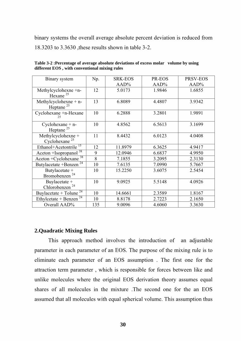
(3-2) Percentage of average absolute deviations of excess molar volume by using different EOS , with conventional mixing rules

30

(3-3) Percentage of average absolute deviations of excess molar volume by using different EOS , with quadratic mixing rules

31

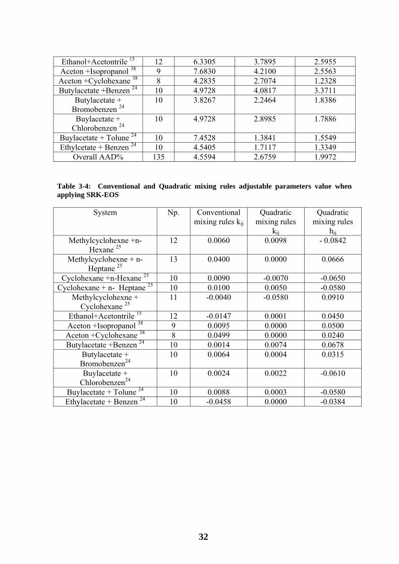
(3-4) Conventional and Quadratic mixing rules adjustable parameters value when applying SRK-EOS

32

(3-5) Conventional and Quadratic mixing rules adjustable parameters value when applying PR-EOS

33

(3-6) Conventional and Quadratic mixing rules adjustable parameters value when applying PRSV-EOS to binary systems

33

(3-7)

(3-8)

(3-9)

Adachi –Sugie mixing rules constants by SRK-EOS to binary systems Adachi –Sugie mixing rules constants by PR-EOS to binary systems Adachi –Sugie mixing rules constants by PRSV-EOS to binary systems

35

35

36

(3-10) Comparison between Adachi-Sugie method of calculating excess molar volume and Modified this method in this work using SRK-EOS

37

IX

(3-11)

(3-12) (3-13)

Modified Adachi –Sugie mixing rules constants by applying PRSV-EOS to Binary systems Modified Adachi –Sugie mixing rules constants by applying PR-EOS to Binary systems Modified Adachi –Sugie mixing rules constants by applying PRSV-EOS to binary systems

37

38

(3-14)

(3-15)

(3-16)

(3-17)

(3-18)

(3-19)

(3-20)

(3-21)

Percentage of average absolute deviations of excess molar volume by using Huron Vidal Method by PRSV-EOS to Binary Systems with the constants The results of ternary system Methylcyclohexane(1) +Cyclohexane(2)+n-Hexane(3) without using adjustable parameter kij=0 The results of ternary system Methylcyclohexane(1) +Cyclohexane(2)+n-Hexane(3) when applying conventional mixing rules The results of ternary system Methylcyclohexane(1) +Cyclohexane(2)+n-Hexane(3) when applying quadratic mixing rules The results of ternary system Methylcyclohexane(1) +Cyclohexane(2)+n-Hexane(3) when applying Adachi-Sugie mixing rules The results of ternary system Methylcyclohexane(1) +Cyclohexane(2)+n-Hexane(3) when applying modified Adachi-Sugie mixing rules in this work The results of ternary system Methylcyclohexane(1) +Cyclohexane(2)+n-Hexane(3) when applying Huron Vidal method The results of ternary system Methylcyclohexane(1) +Cyclohexane(2)+n-Hexane(3) when applying modified Huron Vidal method in this work

37

42

42

42

43

43

43

44

X

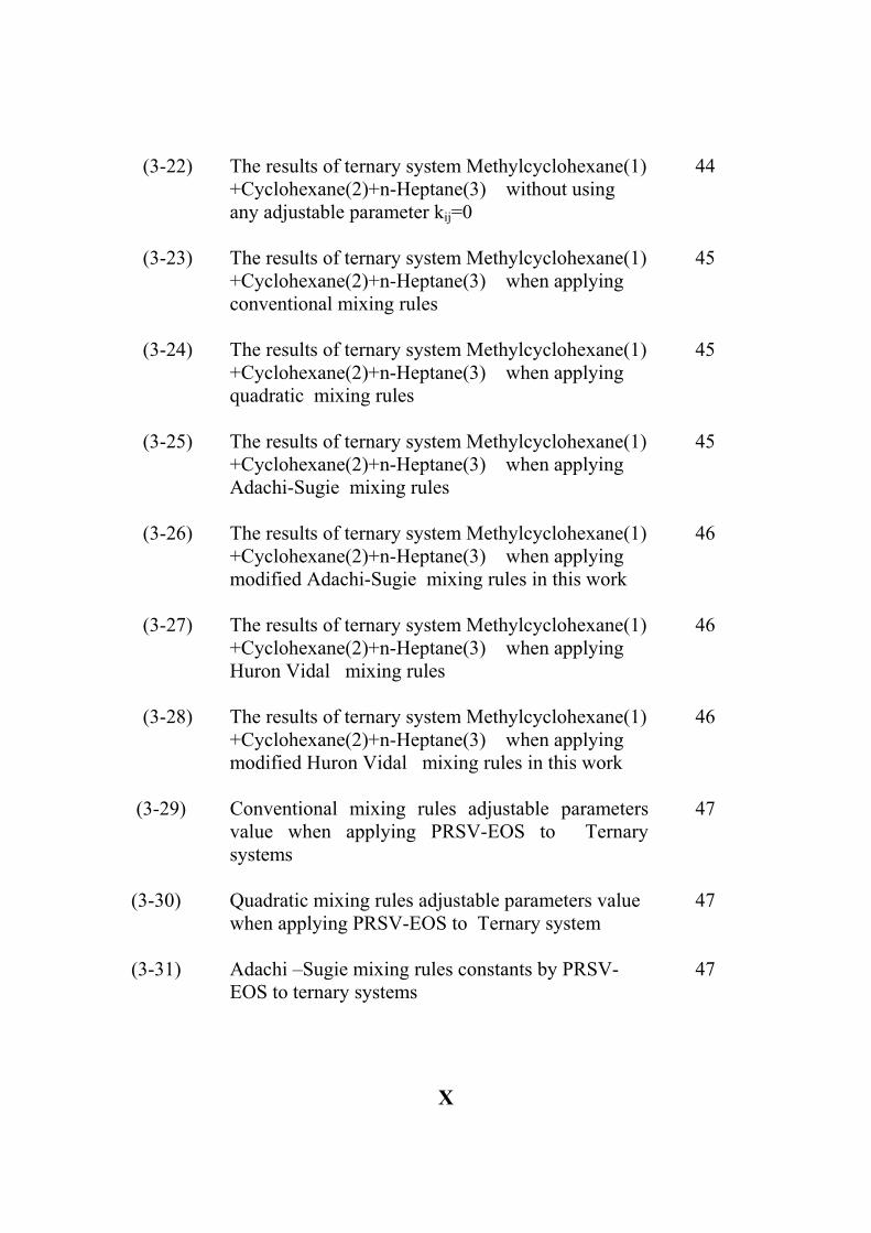
(3-22)

(3-23)

(3-24)

(3-25)

(3-26)

(3-27)

(3-28)

The results of ternary system Methylcyclohexane(1) +Cyclohexane(2)+n-Heptane(3) without using any adjustable parameter kij=0 The results of ternary system Methylcyclohexane(1) +Cyclohexane(2)+n-Heptane(3) when applying conventional mixing rules The results of ternary system Methylcyclohexane(1) +Cyclohexane(2)+n-Heptane(3) when applying quadratic mixing rules The results of ternary system Methylcyclohexane(1) +Cyclohexane(2)+n-Heptane(3) when applying Adachi-Sugie mixing rules The results of ternary system Methylcyclohexane(1) +Cyclohexane(2)+n-Heptane(3) when applying modified Adachi-Sugie mixing rules in this work The results of ternary system Methylcyclohexane(1) +Cyclohexane(2)+n-Heptane(3) when applying Huron Vidal mixing rules The results of ternary system Methylcyclohexane(1) +Cyclohexane(2)+n-Heptane(3) when applying modified Huron Vidal mixing rules in this work

44

45

45

45

46

46

46

(3-29) Conventional mixing rules adjustable parameters value when applying PRSV-EOS to Ternary systems

47

(3-30) Quadratic mixing rules adjustable parameters value when applying PRSV-EOS to Ternary system

47

(3-31) Adachi –Sugie mixing rules constants by PRSV-EOS to ternary systems

47

XI

(3-32) Modified Adachi –Sugie mixing rule constants by applying PRSV-EOS to Ternary systems

47

(3-33) Huron – Vidal Method constant by applying PRSV-EOS to Ternary Systems

48

(3-34) Percentage of average absolute deviations of exces molar volume by using PRSV- EOS for ternary systems

48

(3-35) Percentage of average absolute deviations of excess molar volume by using PRSV-EOS for ternary systems with Huron-Vidal method

48

(4-1) Application of conventional, quadratic, Adachi-Sugie and its modified mixing rules on SRK-EOS for binary systems

54

(4-2) Application of conventional, quadratic, Adachi-Sugie and its modified mixing rules on PR-EOS for binary systems

55

(4-3) Application of conventional, quadratic, Adachi-Sugie and its modified mixing rules on PRSV-EOS for binary systems

55

(4-4) Application of Huron-Vidal method on PRSV-EOS for binary systems

58

(4-5) Application of conventional, quadratic, Adachi-Sugie and its modified mixing rules on PRSV-EOS for ternary systems

59

(4-6) Application of Huron-Vidal method for predictionof excess volume of ternary systems using PRSV-EOS

60

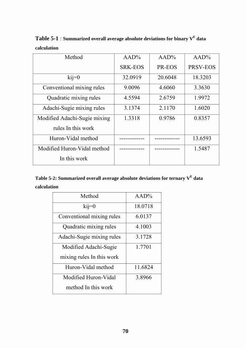
(5-1) Summarized overall average absolute deviations for binary VE data calculation

70

(5-2) Summarized overall average absolute deviations for ternary VE data calculation

70

XII

List of Figures

Figure

Title Page

(2-1) Derivation of (m) relation 15 (4-1) Excess volume of n-Heptane n-Hexane system 57

(4-2) Excess volume of Methylcyclohexane n –Hexane system

60

(4-3) Excess volume of Methylcyclohexane n –Heptane system

61

(4-4) Excess volume of Cyclohexane n –Hexane system 61

(4-5) Excess volume of Cyclohexane n-Heptane system 62

(4-6) Excess volume of Methylcyclohexane Cyclohexane system

62

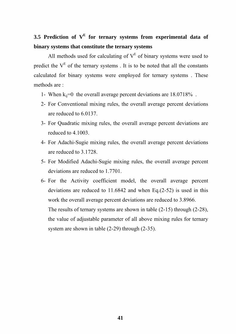
(4-7) Excess volume of Ethanol Acetontrile system 63

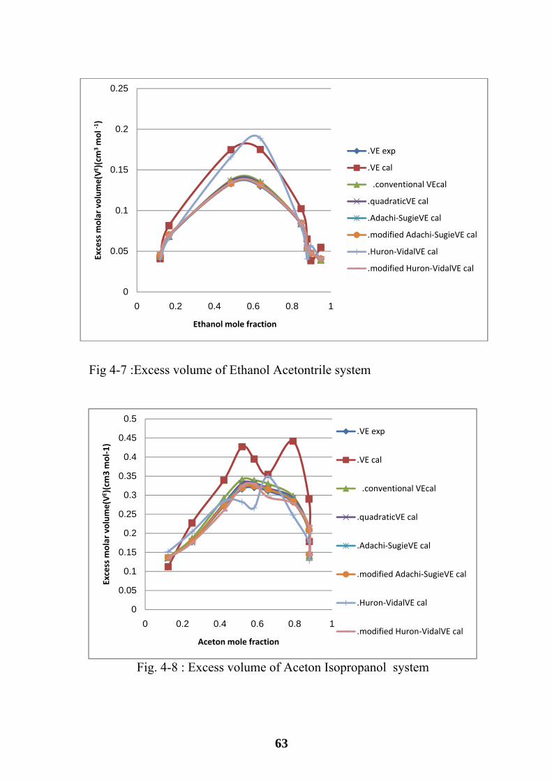
(4-8) Excess volume of Aceton Isopropanol system 63

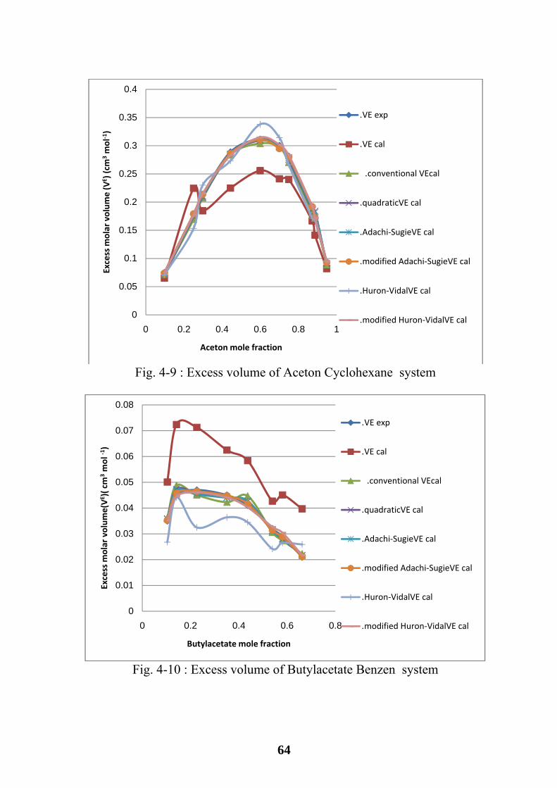
(4-9) Excess volume of Aceton Cyclohexane system 64

(4-10) Excess volume of Butylacetate Benzen system 64

(4-11) Excess volume of Butylacetate Bromobenzen system

65

(4-12) Excess volume of Butylacetate Chlorobenzen system

65

(4-13) Excess volume of Butylacetate Tolune system 66 (4-14) Excess volume of Ethylacetate Benzen system 66

1

Chapter One

Introduction

Excess thermodynamic properties of mixtures correspond to the

differences between the real and the ideal mixing properties, at the same

conditions such as temperature, pressure, composition[1]. The excess thermodynamic property of a binary mixture have gained

much importance in recent years in connection with theories of liquid

mixtures. The excess properties are due to the molecular interactions. They

may be helpful in predicting various physical properties, which are important

in equipment design, engineering and science[2,9]. Excess molar volumes have been measured experimentally by using

the vibrating-tube densimeter and the flow calorimeter device and since it is

difficult to get accurate measurements, researchers tried to find another

suitable way. The researchers tried to calculate molar excess volume (VE) by

making a mathematical model, which fits the experimental data. This

mathematical model is not supported with any theoretical basis. With

development of computers and computer programs, the use of analytical

expression interpolate and even predict thermodynamic information has

become of increasing importance for process design and for modeling of

process operation [17,43].

Because of the long time needed to perform the experimental

measurement of data, their accurate prediction arises to be necessary

objective. In the last few years a considerable efforts have been developed in

order to compile and store the available data in literature d. Despite this work

and the wide literature sources, it is not always possible to obtain proper

values (P-V-T) and the relation between these properties is known as an

2

Equation Of State (EOS). The application of common equations of state for

prediction the excess molar volume, as well as other properties of mixtures

demonstrated that a satisfactory prediction could be obtained also in

multicomponent mixtures by means of mixing rules, where only critical

properties, acentic factor, and other properties values are necessary [23].

The capability of cubic equations of state in correlating excess molar

volume (VE) of non-electrolyte liquid of binary mixture was reported by

several researcher. Djordjevic have shown the satisfactory results for the

calculation of VE of polar and non polar mixtures can be obtained by means

of the one-fluid theory of van der Waals with a single interaction

parameter[11]. In an attempt to improve the correlation of the data for some

non-ideal mixtures, Adachi and Sugie proposed two binary interaction

parameters by using modified conventional mixing rules coupled with van der

Waals (VDW) with Soave(SRK), Peng-Robinson (PR) and Peng-Robinson

Stryjek-Vera(PRSV) [2].

Similarly , Djordjevic and Serbanovic coupled two binary interaction

parameters of the Margules and van laar-type mixing rules with Soave, Peng-

Robinson and Peng-Robinson Stryjek-Vera EOS [12].

The modern development of combining cubic equation of state (CEOS)

with Gibbs free energy models (GE), known as CEOS/GE models, presents a

quite effective method for correlating VLE data of non-ideal systems [16].

Particularly, the HV-NRTL mixing rule coupled with Peng-Robinson

Stryjek-Vera EOS were preliminarily introduced to the analysis of

asymmetric non-polar and polar mixtures. Very satisfactory results are

obtained by means of PRSV-HV-NRTL models parameters are generated

from the experimental VE data [11].

3

The aim of this work is:

1. To evaluate various methods available to correlate and predict excess

molar volume for binary and ternary systems using an equation of state

with suitable mixing rules.

2. To study the effect of the type of equation of state and mixing rules on

the accuracy of correlation and prediction of excess molar volumes for

binary and ternary systems.

3. To predict the excess molar volume for ternary systems based on the

properties of binary systems.

4

Chapter Two

Literature Review

2.1 Law of Corresponding states This law expresses the generalization that the property which is

dependent on intermolecular forces which are related to the critical properties

in the same characteristic way for all compounds. It is the single most

important basis for the development of correlations and estimation methods.

Van der Waals showed that it is theoretically valid for all substances whose

P-V-T properties could be expressed by a two- constant EOS. It is similarly

valid if the intermolecular potential function requires only two parameters.

The relation of pressure to volume at constant temperature is different

for different substances, but if P-V-T is related to the corresponding critical

properties, the function connecting the reduced properties becomes the same

for each substance. Critical temperature, pressure, and volume represent three

widely used pure component constants[5].

The properties (T ,P ,and V) which are measured at the critical point is

called critical temperature, critical pressure and critical volume respectively

and the critical point is the point at which both liquid and gas phase are

coexisting and appears as only one phase. From the law of corresponding

state the compressibility factor at this point is the critical compressibility

factor ( Z [40].

The reduced property is commonly expressed as a function of critical

property:-

Pr= ; Vr= ; Tr= (2-1)

5

An important application of the law of corresponding states is the correlation

of P-V-T using the compressibility factor(Z).

(2-2) ) Z= ,

Which is called law of corresponding states of two parameters. But since

critical compressibility factor (Zc) for many non polar substance is almost

constant near 0.27, so it is assumed for these groups as function of the Tr , Pr

only [1,5].

For highly polar fluids composed of the large molecules the values of

Zc for most hydrocarbons range from 0.2 to 0.3. thus gives a reason for

necessity of using critical compressibility factor (Zc) as additional parameter.

So the law of corresponding states will be of three parameters which is :-

Z= , , (2-3)

However the more common correlation uses the acentric factor (w) as

the third parameter, so

Z= , , (2-4)

For polar compounds and because of their polarity (bonding polarity)

and shape of the molecules the law of corresponding states of three

parameters is not satisfactory, so the law of corresponding states of four

parameters is introduced [22].

Z= , , , (2-5)

2.2 Acentric Factor Pitzar introduces acentric factor in 1955 in order to extend the

applicability of the theorem of corresponding state to normal fluids.

The acentric factor is defined as:

W= -log ( . 1.00 (2- 6)

6

Where P is the reduced saturated vapor pressure at reduced temperature

( =0.7 ). This form is chosen to make w=0 for simple fluids like ( Ar ,Kr

,and Xe) with simple spherical molecules. Hence acentric factor is a factor

that measures deviation of the simple intermolecular potential function from

those values of some substances. However , it should be noted that T =0.7 is

close to the normal boiling point of most substances, thus the particular

choice of T =0.7 adopted by Pitzar not only provides numerical simplicity

because log P =1.0 for simple fluids but also convenience because vapor-

pressure data are most commonly available at pressure near atmospheric [41].

2.3 Intermolecular forces Thermodynamic properties of any pure substance are determined by

intermolecular forces which operate between the molecules of that substance.

Similarly , thermodynamic properties of a mixture depend on intermolecular

forces, which operate between the molecules of the mixture. The case of a

mixture ,however, is necessarily more complicated because consideration

must be given not only to interaction between molecules belonging to the

same component ,but also to interaction between dissimilar molecules. In

order to interpret and correlate thermodynamic properties of solution, it is

therefore necessary to have some understanding of the nature of

intermolecular forces.

The understanding of intermolecular forces is far from complete and

that quantitative results have been obtained for only simple and idealized

models of real matter so, we can use our knowledge of intermolecular forces

only in an approximation manner to interpret and generalized phase-

equilibrium data.

When a molecule is in the approximate of another, forces of attraction

and repulsion strongly influence its behavior. If there were no forces of

7

attraction, gases would not condense to form liquids and soilds, and in the

absence of repulsive forces, condense matter would not show resistance to

compression.

There are many different types of intermolecular forces, these forces

are:-

1. Electrostatic forces between charged particles (ions) and between

permanent dipoles, quadrupoles and multipoles.

2. Induction forces between a permanent dipoles or quadrupole and

induced dipole.

3. Forces of attraction (dispersion forces) and repulsion between non-

polar molecules.

4. Specific (chemical) forces leading to association and complex

formation, i.e. to the formation of loose chemical bonds of which

hydrogen bonds are perhaps the best example [37].

2.4 Excess Volume Excess volume is the thermodynamic property of a solution which is

in excess of those of an ideal solution at the same condition of T, P, and x.

For an ideal mixture all excess volume function are zero. (2-7)

Where V is the molar volume of an ideal solution [37].

2.5 Property Change of Mixing Property change of mixing ,defined as:

M ∑ (2-8)

Where M is any property.

For volume:

∆ ∑ (2-9)

∆

8

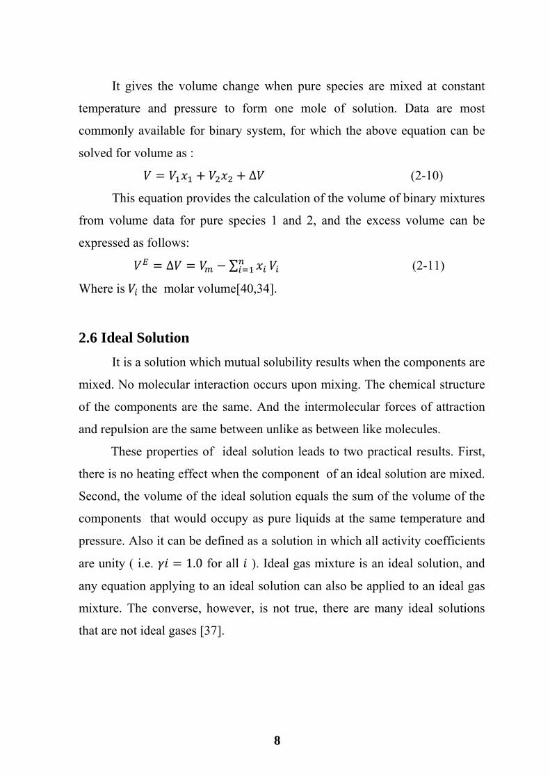
It gives the volume change when pure species are mixed at constant

temperature and pressure to form one mole of solution. Data are most

commonly available for binary system, for which the above equation can be

solved for volume as :

∆ (2-10)

This equation provides the calculation of the volume of binary mixtures

from volume data for pure species 1 and 2, and the excess volume can be

expressed as follows:

∆ ∑ (2-11)

Where is the molar volume[40,34].

2.6 Ideal Solution It is a solution which mutual solubility results when the components are

mixed. No molecular interaction occurs upon mixing. The chemical structure

of the components are the same. And the intermolecular forces of attraction

and repulsion are the same between unlike as between like molecules.

These properties of ideal solution leads to two practical results. First,

there is no heating effect when the component of an ideal solution are mixed.

Second, the volume of the ideal solution equals the sum of the volume of the

components that would occupy as pure liquids at the same temperature and

pressure. Also it can be defined as a solution in which all activity coefficients

are unity ( i.e. 1.0 for all ). Ideal gas mixture is an ideal solution, and

any equation applying to an ideal solution can also be applied to an ideal gas

mixture. The converse, however, is not true, there are many ideal solutions

that are not ideal gases [37].

9

Since the formation of ideal solution results is no change in molecular

energies or volumes, we can write an equation for the volume of an ideal

solution as follows:-

∑ (2-12)

Where is the volume of pure species ( ) at the mixture temperature and

pressure [40].

2.7 Methods of Calculation Molar Excess Volume by Means of

Equation of State Molar Excess Volume can be measured experimentally by using

Suitable densimeter and calorimeter because of difficulties and the error

which are associated with the experiment authors turned attention to calculate

by using EOS.

The calculation of the thermodynamic properties (especially molar

excess molar volume) of mixture have been investigated by using different

methods, these method are :-

1. The Basic Method For binary mixture at constant temperature T and pressure P, the

excess molar volume is calculated by the following equation:- ∑ (2-13)

The molar volume of the mixture and the molar volume of the

components are calculated by using corresponding models of EOS [6,11].

2. The Least Square Method The excess molar volume can be calculated by the following equation:-

1 ∑ 1 2 (2-14)

The values of coefficient are listed in tables for different mixtures [13].

10

3. Redlich-Kister Method The experimental results obtained from the density measurement

are calculated from the following equation: (2-15)

Where , designate ,respectively ,the mole fraction, the density and

the molecular weight, the results obtained from this equation are fitted to the

Redlich- Kister equation.

1 ∑ 1 2 (2-16)

The corresponding coefficient is given in tables for different mixture [2].

2.8 VE Calculation Improvement The main procedure to improve the results from EOS is to improve the

mixing rules. They generally give satisfactory results, but suffer from

common weakness: they fail to describe asymmetric mixture, namely

mixtures constituted by molecules differing very much in size and shape, but

especially in intermolecular force. As a consequence the parameters in the

combining rules lose their physical significance. To overcome these problems, many researchers have turned their

attention towards the development of new mixing rules. All these attempts

can be roughly classified in two categories an empirical mixing rules and

statistical mechanics mixing rules [11].

2.9 Equation of State In the thermodynamic ,an equation of state is a relation between state

variables. More specifically, an equation of state is a thermodynamic equation

describing the state of matter under a given set of physical condition. It is a

constitutive equation which provides a mathematical relationship between two

11

or more state functions associated with the matter, such as its temperature,

pressure, and volume [4]. In the last few years, the interest related to theoretical and

semiempirical work based on equation of state for prediction of excess molar

volume, partial excess molar and partial molar volumes, saturated molar

volumes, vapor-liquid equilibrium or excess molar enthalpies has increased.

This fact is due to its high simplicity as theoretical model, relative accuracy,

low information requirements, and wide versatility in operation conditions

[33].

The most prominent use of an equation of state is to predict the state of

gases and liquids. One of the simplest equation of state for this purpose is the

ideal gas low, which is roughly accurate for gases at low pressure and high

temperature. However, this equation becomes increasingly inaccurate at

higher pressures and low temperature, and fails to predict condensation from a

gas to a liquid. Therefore, a number of much more accurate equations of state

have been developed for gases and liquids. At present, there is no single

equation of state that accurately predicts the propertied of all substances under

all conditions [4].

Many equations of state have been proposed and each year additional

ones appear in the technical literature, but almost of all them are essentially

empirical in nature. A few (e.g. the equation of van der Waals ) has at least

some theoretical basis, but all empirical equations of state for a pure gas have

at least only approximate physical significance. It is very difficult (and

frequently impossible) to justify mixing rules for expressing the constants of

the mixture in terms of the constants of the pure components which comprise

the mixture. As a result, such relationship introduces further arbitrary

empirical equations of state one set of mixing rules may work for. One or

several mixtures but work poorly for others.

12

The constants which appear in a gas or liquid phase equation of state

reflect the non-ideality of the gas and liquid, the fact that there is a need for

any constants at all follows from the existence of intermolecular forces.

Therefore, to establish the composition dependence of the constant (i.e.

mixing rules), it is important that the constants in an equation of state have a

clear physical significance. For reliable results, it is desirable to have a

theoretically meaningful equation of state in order that mixture properties may

be related to pure – component properties with a minimum of

arbitrariness[37].

2.10 Classification of Equation of State The need for accurate prediction of the thermodynamic properties of

many fluids and mixtures has led to the development of a rich diversity of

equations of state with different degrees of empiricism, predictive capability

and mathematical form. Before processing with the discussion of specific

equations of state it is useful to make some general classifications into which

they may fall.

The main types of EOS may be classified conveniently according to

their mathematical form as follows:-

Standard P-V-T forms:

This type of EOS may be written for pure fluids

As

, or , (2-17)

While for mixture of 'n' components, there are a further 'n-1'

independent composition variables. Sub-classifications may be introduced

according to the structure of the function or :

13

Ι. Truncated virial equation in which P is given by a polynomial in 1/ with

temperature and composition dependent coefficients.

Π. Cubic equations in which P is given by a cubic function of containing

two parameters which are functions of composition and possibly also of

temperature.

ΠΙ.Complex empirical equation which represent P by some combination of

polynomial and other terms[30].

2.11 Cubic Equation of State Engineers must often perform complex phase – equilibria calculations

to model systems typically found in the refining and chemical industries.

Cubic equations of state (CEOS) are currently the equation of state considered

most applicable for such calculations. This article focuses on the enhancement

made to the CEOS that are considered industry-wide standards and points out

the strengths and limitations of these CEOS and their mixing rules [21]. For an accurate description of the PVT behavior of fluids over wide

ranges of temperature and pressure, an EOS required. Such an equation must

be sufficiently general to apply to liquids as well as gases and vapors.

The first practical cubic EOS was proposed by J.D. van der Waals in

1873.

(2-18)

Here 'a' and 'b' are positive constants where 'b' is related to the size of the

hard sphere while 'a' can be regarded as measured of the intermolecular

attraction force [42].

For correlation and prediction of excess molar volume for binary and

ternary mixtures the following well-known cubic equations of state were

used :

14

2.11.1 Soave Redlich Kwong Equation Of State (SRK-EOS) Soave in (1972)successfully developed a generalized alpha function

" " for cubic equation of state which made the parameter ' ' function of

reduced temperature ( , and accentic factor (w) [i.e. , , ].

Soave calculated the values of " " at a series of temperature for a

number of pure hydrocarbons, using the equality of vapor and liquid

fugacities along the saturation curve. The fugacity of each component in a

mixture is identical in all phases at equilibrium. This is equally true for a

single component system having vapor and liquid phases at equilibrium.

In this case,

(2-19)

This equation is valid at any point on the saturation curve, where the vapor

and liquid coexist in equilibrium.

Soave calculated the values of " " over a temperature range of

0.4 to 1.0 for a number of light hydrocarbons and found that . was a

liner function of . with a negative slope for each fluid studied Fig.1-1

shows this relation and it is represented by the following equation

. . (2-20)

Because 1.0 at 1.0, by definition where

(2-21)

So ,Eq.(2-20) may be written as follows

. 1 1 . (2-22)

To obtain the value of 'm' it was calculated for a series of " " values from 0

to 0.5 with an interval of 0.05, and then correlated as a quadratic function of

" ", as follows [41,48].

=0.48 1.574 0.176 (2-23)

15

So, Soave replaced / . of Redlich Kwong equation by and the,

equation of state became as:

(2-24)

Eq.(2-24) in polynomial form in Z factor is

0 (2-25)

Fig. 1-1 : Derivation of (m) relation 1

2.11.1.1 SRK-EOS Parameters: Soave predicated a new method for determining the new equation

parameters as follows:[41]

1 1 . (2-26)

And since 0.48 1.574 0.176 (2-27)

0.42748 (2-28)

And since (2-29)

The second parameters was calculated as follows:

16

0.08664 (2-30)

(2-31)

(2-32)

2.11.2 Peng-Robinson Equation of State (PR-EOS) Peng-Robinson (PR) proposed an equation of the form:

(2-33)

Rearranging Equation (2-33) in cubic form in terms of V gives

3 0 (2-34)

In PR-EOS "a" is also of " " and " " function is:

. 1 1 . (2-35)

Where "k" is a constant that has been correlated against the acentric factor.

The resulting k equation is

0.37464 1.54226 0.26992 (2-36)

Both Soave and Peng-Robinson equations are excellent in predicting the

vapor pressure. This important capability terms from the remarkably good

expressions for " " Eq. (2-23) for Soave modification, and Eq.(2-36) for

Peng-Robinson equation, rather than from the formulation of the EOS. But

the form of EOS does effect the predicting of molar volumes in the dense

phase region, where PR equation, although not as accurate as desired, shows a

mark improvement over the Soave equation [52].

The Peng-Robinson equation was developed in 1976 in order to satisfy

the following goals:

17

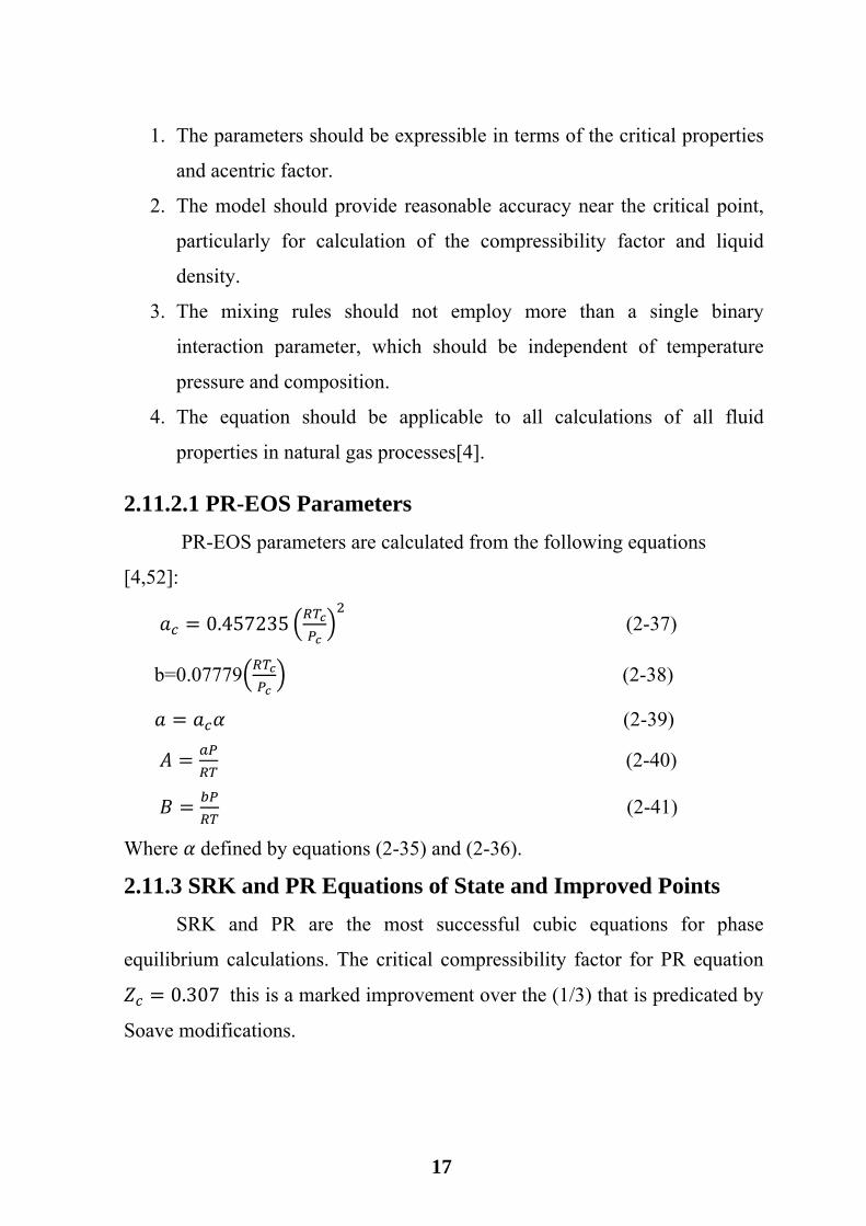
1. The parameters should be expressible in terms of the critical properties

and acentric factor.

2. The model should provide reasonable accuracy near the critical point,

particularly for calculation of the compressibility factor and liquid

density.

3. The mixing rules should not employ more than a single binary

interaction parameter, which should be independent of temperature

pressure and composition.

4. The equation should be applicable to all calculations of all fluid

properties in natural gas processes[4].

2.11.2.1 PR-EOS Parameters PR-EOS parameters are calculated from the following equations

[4,52]:

0.457235 (2-37)

b=0.07779 (2-38)

(2-39)

(2-40)

(2-41)

Where defined by equations (2-35) and (2-36).

2.11.3 SRK and PR Equations of State and Improved Points SRK and PR are the most successful cubic equations for phase

equilibrium calculations. The critical compressibility factor for PR equation

0.307 this is a marked improvement over the (1/3) that is predicated by

Soave modifications.

18

However, the value is still far from the actual critical compressibility

factor of real fluids except for Hydrogen and Helium. On the other hand the

failure point of both Soave and Peng-Robinson equation is the assumption of

a particular (fixed) value of the critical compressibility factor and, as a result,

the predicated densities of the saturated liquids and the predicated critical

volumes differ considerably from their experimental values especially for

substances whose critical compressibilities are significantly different from the

values assumed by these equations [12,52].

2.11.4 Peng-Robinson-Stryjek-Vera Equation In this work a complete overview the results that can be obtained with

a modified Peng-Robinson equation of state, called the PRSV equation is

represented . Although in many represents the modifications introduced in the

PRSV (Stryjek and Vera.1986) follow ideas of previous workers in the details

are significant enough to produce a definite improvement with respect to

other versions of cubic equation of state. Vapor-liquid equilibria of many

binary systems are well represented with standard one-binary parameter

mixing rules. The cases for which the use of two binary parameters is required

are indentified. These cases will be treated with more detail in PRSV

equation[3,44].

Peng-Robinson Stryjek-Vera(PRSV)EOS[3]:

3 2

0 (2-42)

PRSV-EOS has the potential to predict more accurately the phase

behavior of hydrocarbon systems, particularly for system composed of

dissimilar components, and it can also be extended to handle non-ideal

system with accuracies that rival traditional activity coefficient models. The

19

only compromise is increased computational time and the additional

interaction parameter that is required for the equation[52].

2.11.4.1 PRSV Parameters 0.077796 ⁄ (2-43)

0.457235 ⁄ (2-44)

1 1 . (2-45)

1 . 0.7 (2-46)

0.378893 1.4897153 0.17131848

0.0196554 (2-47)

was considered to be a function of the acentric factor and being an

adjustable parameter characteristic of each pure compounds given by Stryjek

and Vera [6,43,44,46].

2.12 Application of Cubic Equation of State to Mixtures Up to now, mixture properties usually predicted by a cubic EOS

together with appropriate mixing rules. The most important use of EOS is

perhaps as thermodynamic property generators in chemical process

simulators. Current simulator architectures are moving away from the

traditional sequential modular to equation-oriented and simultaneous modular.

Equation of state that yield simple analytical expression and deveratives for

thermodynamic properties are desirable. For both theoretical and practical

points of view, mixing rules are most useful when they:

1. are simple,

2. avoid excessive use of parameters,

3. require a light computational load for mixtures with many compounds,

4. are reduced to the classical mixing rulers for simple mixtures,

20

5. perform well for asymmetric non-polar mixtures, and

6. obay the quadratic dependency on composition of the second virial

coefficient at low density limits.

Many modifications and improvements of the van der Waals type

equations of state appear in the literature. These modifications incorporate

new parameters to the equation and/or modify the classical mixing rules[12].

There are two basic concepts in the developing of mixing rules which

are :

1. Empirical Mixing Rules Mixing rules play a fundamental role in extending an equation of state

to mixture properties calculations, and the results obtained will depend, to a

higher extent, on the selection mode. Consequently, the study of combination

of different forms of mixing rules, and the applicability to the mixtures,

related to the nature of the components, arises to be essential [19]. The basic concept in developing a mixing rules is to use an equation

giving satisfactory results in modeling the fluid state, and then to extend it to

high pressure calculations, and the vapor phases. Most models successfully

describing the liquid phase are based on local composition concept: they are

flexible enough to describe the complex behavior exhibited by system

containing polar compounds. Suffice it to say that it can quantitatively

describe mixtures where non-randomness is involved.

The first attempts to introduce the local composition concept in EOS

were empirical : Heyen[19] and Vidal[51].Although their approaches

represented a significant advance in modeling complex mixture phase

equilibria , they suffer from several shortcomings . The parameters have no

physical significance and do not depend on density [29].

21

2. Statistical Mixing Rules Local composition can also be derived from statistical thermodynamic

and examined by using computer generator data for model fluids. In spite of success of some researchers in describing mixtures of real

fluids, the rigorous statistical mechanics treatment of complex system for

which excess Gibbs free energy ( models have customarily been used is

not near ,on the other hand, empiricism should be introduced at some point in

the development. This theoretical approach, however, will be very useful in

developing more theoretical based function relationships for treatment of real

fluids [5,29].

2.13 Introduction of Mixing and Combining Rules to Improve

VE calculation The introduction of new mixing and combining rules is very important

in order to improve EOS mixing rules and as a result improve VE calculated

results. Many researchers and authors introduce different forms of

mixing and combining rules as presented in the following sub-

section.

2.13.1 Conventional One-Binary-Parameter Form In order to examine the effect of the number of binary interaction

parameters, present in this type of mixing rules, and of their position in

various parameters, several forms of van der Waals mixing rules were tested.

The energy parameters , present in the original two parameter van der

Waals one-fluid mixing rules( vdW1), which is a quadratic dependence

on composition, can be expressed by the following equation:

∑ ∑ (2-48)

22

Where , the cross interaction coefficient , has the form

. 1 (2-49)

In this equation , and are the parameters of pure component ,

whereas denotes the binary interaction parameter or adjustable parameter

is a binary constant, small compared to unity, characterizing the

interaction between molecules 'i' and 'j' . For most non-polar systems kij is

essential independent of composition . Interaction parameter can be positive

or negative, but it is seldom gives quantitative good results. The

parameter is especially significant for system containing chemically

dissimilar components. However, even for systems of chemically similar

components , different from zero as a result of difference in molecular

shapes and size [14] .

This adjustable parameter tries to decreases the error that might be

associated with EOS and shifts the results to higher degree of accuracy.

The covolume parameter b is given by the linear composition

dependence in the form

∑ (2-50)

The conventional one binary parameter combining rule in all case

produce not so accurate results for calculation. Such rules may be used for

low density components and regular solution, such as approximate similar

components in hydrocarbon mixtures . In presence of polar compounds they

must be improved by introducing empirical correction terms [16].

2.13.2 Quadratic Two – Binary –Parameter Form The second modification to mixing rules in order to apply to mixture is

required in the presence of dissimilar hydrocarbon mixtures which are greatly

differ in their structure and the case of presence polar compounds .

Conventional mixing rules are no more adequate . A high degree of flexibility

23

must be given , for instance by an extension of the linear law of covolume

parameter ′ ′ to a quadratic rule , and the introduction of a second empirical

binary constant : ∑ ∑ (2-51)

The cross interaction parameter is defined by the following equation:-

1 (2-52)

Where is a second binary interaction parameter used to terminate the

error associated with similarity assumption of mixture components shape and

size.

Such rules, although theoretically well supported and completely

adequate for binary systems , yet fail when applied to multicomponent

mixture . It is likely more complicated rules , involving ternary and higher

order terms have to be considered , but it is an impractical route , awing to the

extremely large number of terms and long computation times involved

[16,34].

2.13.3 Adachi– Sugie Type Two– Binary–Parameter Form In order to increase the results accuracy obtained from any EOS used

adjustable parameters which are proposed by Y. Adachi and H. Sugie may be

applied.With a linear mixing rule for a covolume parameter ′ ′ of a cubic

EOS, the calculation of thermodynamic property depends on cohesion

parameter ′ ′ only at specific temperature, pressure, and mole fraction (x).

Any thermodynamic property calculation is strongly depending on the binary

interaction parameters of the modified conventional mixing rules expressed as ∑ ∑ (2-48)

. 1 (2-49)

(2-53)

24

Where and are binary interaction parameters , are mole fractions

of component 'i' and 'j' respectively [16].

2.13.4 Huron and Vidal Mixing Rules (HV- Mixing Rules)

It is well known that a good reproduction of the VE behavior

of mixture containing polar components can be obtained only with parameter

mixing rule with a high degree of flexibility , i.e. containing a sufficient

number (at least two) of adjustable binary parameters [50]. Very recently some mixing rules combining free energy model (GE)

and equation of state (EOS) have been successfully applied to very complex

system of diversified nature covering wide ranges of temperature and pressure

. Among of these models the so – called EOS/GE that has been used for the

correlation and prediction of VE and other thermodynamic properties . These

models have been widely studied and an extensive analysis for their

applicability has been reviewed in several excellent articles . EOS mixing rules , based on local composition concepts for excess Gibbs

energy , were introduced by Huron and Vidal which opened away to rich

field of the liquid state theories [22] .

The Huron and Vidal mixing rules is successful in combination with a

model of Non Random Two Liquids equation (NRTL). This equation was

chosen as an activity coefficient model for the calculation of the excess Gibbs

energy (GE) . The NRTL equation can be expressed by the equation [3,37] :

In general:

∑ ∑

∑ (2-54)

For binary systems

(2-55)

25

For ternary systems

(2-56)

Where

exp exp (2-57)

∆ ∆ (2-58)

∆ (2-59)

∆ (2-60)

∑ (2-61)

Where

1 √2 (2-62)

, (2-63)

26

Chapter Three

Investigation and development of the correlation and

prediction of excess molar volume for binary and

ternary systems 3.1 Why Selecting The Redich Kwong (RK) EOS Family ?

The first historical reason is that , when a systematic work on EOS was

began , the only available EOS combining ease of treatment and accuracy was

those equations of states , which derived from RK equation. Cubic nature

made is very practical to use , and unlike second order virial equations it

could be applied to liquid phase also[50] .

The RK-EOS and its derivatives equations they remain until now as the

better of all two parameter cubic equations .

To know the applicability and accuracy of any proposed correlation it

is very important to know how this correlation fits the experimental data

which is done by comparing the obtained results from the proposed

correlation with the experimental data.

The accuracy of proposed correlations is determined by the following

methods:

1.Absolute percent of deviation (AD%E)

. % = 100% (3-1)

2. Average Absolute Percent Deviation (AAD%)

% ∑ .% (3-2)

27

Where n is the number of data points.

3.2 Selecting of an EOS for Excess Molar Volume Calculation and

prediction

The interest in the prediction of the thermodynamic properties from

equations of state has remarkably increased in the last few year The fact can

be explained by the wide range of applicability equation of state in industrial

operation conditions. Recently, cubic equation of state become very powerful

in correlating and predicting phase equilibrium behavior for either no polar or

/ and polar systems. This capability comes from the ability of predicting pure

component vapor pressure accurately for polar and nonpolar components .

In this work three types of cubic equations of state were used to

calculate VE of binary mixture and these equations are Soave Redlich Kwong

(SRK) equation , Peng Robinson (PR) equation , and Peng Robinson stryjek

Vera (PRSV) equation while the PRSV equation of state was used to

calculate VE for the ternary mixtures .

Each of the above equations were applied to fourteen binary mixture.

The results obtained by calculation as compared with experimental data are

shown in table 3-1 .These results were obtained when the mixing rules of the

three equations were not changed and no adjustable parameter or interaction

parameter were used i,e kij=0 .

Table 3-1 shows that PR and PRSV equations of state give

approximately the same results or approximately the same deviations from

experimental excess molar volume data . On the other hand SRK equation

gives relatively larger deviations than those obtained by either PR or PRSV

equation of state . As table 3-1 indicates the overall absolute average percent

deviation of using SRK , PR and PRSV are 32.0919 , 20.6048 and 18.3203

28

respectively . These high deviations in the results are certainly due either to

the poor mixing rules or the equations of state used.

Although the deviations from experimental data are high but the results

proved that equations of state which were used are capable of calculating

excess molar volume of a mixture because there are direct relation between

VE obtained by calculation and experimental VE. In order to improve the

accuracy of VE results , mixing rules have to be modified by introducing one

or more adjustable parameter.

Table 3-1: Percentage of average absolute deviations of excess molar volume by using different EOS , with kij=0

PRSV AAD% PR AAD% SRK AAD% Np. System 0.5986 0.8555 1.2979 23 n-Heptane +n-Hexane 27 14.1354 16.1283 22.2803 12 Methylcyclohexne +n-

Hexane 25 16.4921 18.0327 22.4074 13 Methylcyclohexne + n-

Heptane 25 12.8980 14.8004 20.8733 10 Cyclohexane +n-Hexane 25 17.7669 19.2928 25.4975 10 Cyclohexane + n-

Heptane 25 15.6199 18.0201 22.8341 11 Methylcyclohexne +

Cyclohexane 25 30.0441 33.7668 38.9029 12 Ethanol+Acetontrile 15 21.7456 252413 39.5962 9 Aceton +Isopropanol 38 20.1580 23.6669 40.9559 8 Aceton +Cyclohexane 38 33.4363 36.2130 51.4665 10 Butylacetate +Benzen 24 28.7295 30.9373 43.2673 10 Butylacetate +

Bromobenzen 24 24.2225 26.6494 49.5700 10 Buylacetate +

Chlorobenzen 24 20.0593 22.2179 59.2195 10 Buylacetate + Tolune 24 23.6356 28.6894 58.1057 10 Ethylcetate + Benzen 24 18.3203 20.6048 32.0919 158 Overall AAD%

29

3.3 Applying Different Mixing Rules on the Selected EOS

Different forms of mixing rules were applied to binary and ternary

mixtures. Investigation of the abilility of these forms of mixing and

combining rules to predict VE data and hydrocarbon systems and to find the

most suitable one to be used with SRK, PR, and PRSV equations. When

applying these forms of mixing and combining rules for VE .The success of

the correlations depends on the accuracy of the EOS used and on the mixing

rules at one hand ; and the accuracy of experimental data point at the other

hand. These forms of mixing and combining rules are :

1. Conventional Mixing Rules

The oldest method used to improve the excess molar volume results

obtained by using an EOS and conventional mixing rules with an adjustable

parameter (kij) which introduced in the attraction term of an EOS. The

method used for determining kij by using minimizing objective function (OF)

method given by Eq. (3-3) which has the form .

∑ (3-3)

Where kij value is the value which gives the lowest VE deviation from

experimental value kij value is introduced in the attraction term "a" parameter

of an EOS as described by Eq. (2-49)

. 1 (2-49)

This introduction of an adjustable parameter improves the EOS mixing

rules and consequently reduces the error of calculated VE . Where for SRK–

EOS binary systems the overall average absolute percent deviation is reduced

from 32.0919 to 9.0774 while for PR-EOS the overall average absolute

percent deviation is reduced from 20.6060 to 4.6060 and for PRSV-EOS

30

binary systems the overall average absolute percent deviation is reduced from

18.3203 to 3.3630 ,these results shown in table 3-2.

Table 3-2 :Percentage of average absolute deviations of excess molar volume by using different EOS , with conventional mixing rules

PRSV-EOS AAD%

PR-EOS AAD%

SRK-EOS AAD%

Np. Binary system

1.6855 1.9846 5.0173 12 Methylcyclohexne +n- Hexane 25

3.9342 4.4807 6.8089 13 Methylcyclohexne + n-Heptane 25

1.9891 3.2801 6.2888 10 Cyclohexane +n-Hexane 25

3.1699 6.5613 4.8562 10 Cyclohexane + n- Heptane 25

4.0408 6.0123 8.4432 11 Methylcyclohexne + Cyclohexane 25

4.9417 6.3625 11.8979 12 Ethanol+Acetontrile 15 4.9950 6.6837 12.0946 9 Aceton +Isopropanol 38 2.3130 3.2095 7.1855 8 Aceton +Cyclohexane 38 5.7667 7.0990 7.6135 10 Butylacetate +Benzen 24 2.5454 3.6075 15.2250 10 Butylacetate +



2.Quadratic Mixing Rules

This approach method involves the introduction of an adjustable

parameter in each parameter of an EOS. The purpose of the mixing rule is to

eliminate each parameter of an EOS assumption . The first one for the

attraction term parameter , which is responsible for forces between like and

unlike molecules where the original EOS derivation theory assumes equal

shares of all molecules in the mixture .The second one for the an EOS

assumed that all molecules with equal spherical volume. This assumption thus

31

corrected this term by the introduction of a new adjustable parameter hij in the

co volume EOS parameter which eliminates the error associated with this

assumption . This adjustable parameter improves the results significantly for

mixtures components which have shape far from spherical shape. The

quadratic mixing rules have the form :

∑ ∑ (2-48) . 1 (2-49)

∑ ∑ (2-50)

1 (2-51)

Where kij and hij are adjustable parameters in the attraction and co

volume terms respectively . The overall average absolute percent deviation

for SRK –EOS reduced to 4.5594 , for PR-EOS the overall average absolute

percent deviation reduced to 2.6759 while for PRSV-EOS the overall average

absolute percent deviation for binary systems is reduced to 1.9972 these

results shown in table 3-3, also the values of adjustable parameters in

conventional and quadratic mixing rules are given in tables 3-4, 3-5 , 3-6.

Table 3-3: Percentage of average absolute deviations of excess molar volume by using different EOS , with quadratic mixing rules

PRSV-EOS AAD%

PR-EOS AAD%

SRK-EOS AAD%

Np. Binary system

0.8450 0.9652 2.5896 12 Methylcyclohexne +n- Hexane 25




3.0765 3.5586 4.8428 11 Methylcyclohexne + Cyclohexane 25

32

2.5955 3.7895 6.3305 12 Ethanol+Acetontrile 15 2.5563 4.2100 7.6830 9 Aceton +Isopropanol 38 1.2328 2.7074 4.2835 8 Aceton +Cyclohexane 38 3.3711 4.0817 4.9728 10 Butylacetate +Benzen 24 1.8386 2.2464 3.8267 10 Butylacetate +



Table 3-4: Conventional and Quadratic mixing rules adjustable parameters value when applying SRK-EOS

System Np. Conventional mixing rules kij

Quadratic mixing rules

kij


hij Methylcyclohexne +n-

Hexane 25 12 0.0060 0.0098 - 0.0842

Methylcyclohexne + n-Heptane 25

13 0.0400 0.0000 0.0666

Cyclohexane +n-Hexane 25 10 0.0090 -0.0070 -0.0650 Cyclohexane + n- Heptane 25 10 0.0100 0.0050 -0.0580

Methylcyclohexne + Cyclohexane 25

11 -0.0040 -0.0580 0.0910

Ethanol+Acetontrile 15 12 -0.0147 0.0001 0.0450 Aceton +Isopropanol 38 9 0.0095 0.0000 0.0500 Aceton +Cyclohexane 38 8 0.0499 0.0000 0.0240 Butylacetate +Benzen 24 10 0.0014 0.0074 0.0678

Butylacetate + Bromobenzen24

10 0.0064 0.0004 0.0315

Buylacetate + Chlorobenzen24

10 0.0024 0.0022 -0.0610

Buylacetate + Tolune 24 10 0.0088 0.0003 -0.0580 Ethylacetate + Benzen 24 10 -0.0458 0.0000 -0.0384

33

Table 3-5: Conventional and Quadratic mixing rules adjustable parameters value when applying PR-EOS



kij



Hexane 25 12 0.0084 -0.0058 0.0190


13 0.0032 0.0080 0.0432

Cyclohexane +n-Hexane 25 10 -0.0020 -0.0624 0.0530 Cyclohexane + n- Heptane 25 10 0.0340 0.0027 0.0850


11 0.0860 0.0000 -0.0650

Ethanol+Acetontrile 15 12 0.0020 -0.0050 0.0590 Aceton +Isopropanol 38 9 -0.0010 0.0090 -0.0300 Aceton +Cyclohexane 38 8 0.0230 0.0300 -0.0560 Butylacetate +Benzen 24 10 -0.0790 0.0000 -0.0180


10 0.0120 -0.0050 0.0380


10 0.0803 0.000 0.0160

Buylacetate + Tolune 24 10 -0.0053 -0.0060 0.0390 Ethylacetate + Benzen 24 10 0.0858 -0.0319 0.0129

Table 3-6: Conventional and Quadratic mixing rules adjustable parameters value when applying PRSV-EOS to binary systems



kij



Hexane 25 12 0.0047 0.0000 0.0854


13 0.0050 -0.0392 0.0920

Cyclohexane +n-Hexane 25 10 -0.0560 0.0024 0.0938 Cyclohexane + n- Heptane 25 10 0.0059 0.0080 -0.0473


11 0.0044 -0.0009 0.0537

Ethanol+Acetontrile 15 12 -0.0039 0.0020 0.0150 Aceton +Isopropanol 38 9 0.0480 -0.0350 0.0900 Aceton +Cyclohexane 38 8 0.0440 0.0080 0.0230 Butylacetate +Benzen 24 10 0.0065 0.0040 0.0860


10 0.0210 -0.0081 0.0226


10 - 0.0480 0.0007 - 0.0930

34

Buylacetate + Tolune 24 10 0.0831 0.0096 0.0161 Ethylacetate + Benzen 24 10 0.0595 -0.0010 0.0160

3. Adachi-Sugie Mixing Rules

In this approach method Adachi-Sugie (AS) increased the accuracy of

VE results obtained from any EOS by using binary adjustable parameters in

attraction term of an EOS which combines a CEOS for VE data and

correlation method . AS-mixing rules has the form

. 1 (2-49)

∑ ∑ (2-51)

(2-53)

Adachi and Sugie directed their efforts on eliminating the errors resulted from

the attraction term parameter . They discovered that an EOS is more sensitive

to any changes in the value of "a" parameter than the change in the "b"

parameter. They related the adjustable parameter to composition and two new

adjustable parameters that are introduced which are Lij and mij respectively.

The value of Lij and mij for all systems used are shown in table 3-7 through

3-9. The overall average percent deviations for SRK-EOS are reduced to

3.1374, for PR-EOS are reduced to 2.1170 and the overall average percent

deviations for PRSV-EOS to binary systems are reduced to 1.6020. These

results are shown in table 3-10.

35

Table 3-7: Adachi –Sugie mixing rules constants by SRK-EOS to binary Systems

Systems Np. Lij mijMethylcyclohexne +n- Hexane25 12 -0.0004 0.0065

Methylcyclohexne + n-Heptane25

13 -0.0243 0.0505

Cyclohexane +n-Hexane 25 10 0.0083 0.0547 Cyclohexane + n- Heptane 25 10 0.0010 0.0530


11 -0.0196 0.0643

Ethanol+Acetontrile 15 12 0.047 -0.0095 Aceton +Isopropanol 38 9 0.0040 -0.0155 Aceton +Cyclohexane 38 8 0.0083 -0.0726 Butylacetate +Benzen 24 10 -0.0330 0.0058

Butylacetate + Bromobenzen 24 10 0.0152 0.0094 Buylacetate + Chlorobenzen 24 10 -0.0018 0.0007

Buylacetate + Tolune 24 10 0.0009 0.0011 Ethylacetate + Benzen 24 10 0.0092 0.0232

Table 3-8: Adachi –Sugie mixing rules constants by PR-EOS to binary Systems

Systems Np. Lij mijMethylcyclohexne +n- Hexane25 12 0.0282 0.0068


13 0.0732 -0.0058

Cyclohexane +n-Hexane 25 10 0.0073 0.0148 Cyclohexane + n- Heptane 25 10 0.0846 -0.0050


11 0.0268 -0.0809

Ethanol+Acetontrile 15 12 -0.0387 0.0078 Aceton +Isopropanol 38 9 0.0112 0.0088 Aceton +Cyclohexane 38 8 -0.0091 0.0045 Butylacetate +Benzen 24 10 0.0017 0.0501

Butylacetate + Bromobenzen 24 10 0.0112 -0.0068 Buylacetate + Chlorobenzen 24 10 0.0529 0.0740

Buylacetate + Tolune 24 10 -0.0514 0.0090 Ethylacetate + Benzen 24 10 0.0070 -0.0620

36

Table 3-9: Adachi –Sugie mixing rules constants by PRSV-EOS to binary Systems

Systems Np. Lij mijMethylcyclohexne +n- Hexane25 12 0.0088 -0.0100


13 -0.0849 0.0432

Cyclohexane +n-Hexane 25 10 -0.0848 0.0320 Cyclohexane + n- Heptane 25 10 -0.0705 0.0038


11 0.0018 -0.0064

Ethanol+Acetontrile 15 12 0.0160 0.0670 Aceton +Isopropanol 38 9 -0.0950 0.0020 Aceton +Cyclohexane 38 8 -0.0280 0.0300 Butylacetate +Benzen 24 10 0.0785 - 0.0047

Butylacetate + Bromobenzen 24 10 -0.0089 0.0321 Buylacetate + Chlorobenzen 24 10 0.0050 0.0100

Buylacetate + Tolune 24 10 0.0193 -0.0499 Ethylacetate + Benzen 24 10 -0.0690 0.0503

4.Modification of Adachi –Sugie Mixing Rules

In this work Adachi –Sugie mixing rules are modified by using three

adjustable parameter Lij, mijin attraction and repulsion terms " " and "b"

which has the form :

. 1 (2-49)

∑ ∑ (2-51)

(2-53)

1 (2-52)

This method gives more accurate results of VE. The overall average percent

deviations for SRK-EOS are reduced to 1.3318, for PR-EOS are reduced to

0.9586 and for PRSV-EOS to binary systems are reduced to 0.8235. These

results are shown in table 3-8. The values of Lij, mij and hij for all systems

used are shown in the table 3-11 through 3-13.

37

Table 3-10: Comparison between Adachi-Sugie method of calculating excess molar volume and Modified this method in this work using SRK-EOS

Table 3-11:Modified Adachi –Sugie mixing rules constants by applying SRK-EOS to Binary systems

hij Mij Lij Np. System

0.0340 -0.0158 0.0050 12 Methylcyclohexne +n- Hexane 25


0.0.0470 0.0006 0.0118 10 Cyclohexane +n-Hexane 25 -0.0740 0.0028 -0.0080 10 Cyclohexane + n-

Heptane 25 -0.0390 -0.0156 0.0600 11 Methylcyclohexne +

Cyclohexane 25 -0.0413 0.0095 -0.0369 12 Ethanol+Acetontrile 15 0.0200 -0.0817 0.0118 9 Aceton +Isopropanol 38 -0.0350 0.0622 0.0050 8 Aceton +Cyclohexane 38 -0.0920 0.0038 0.0008 10 Butylacetate +Benzen 24

This work AAD%

Adachi-Sugie method AAD%

Np. Binary system

0.5451 2.0258 12 Methylcyclohexne +n- Hexane 25

0.8894 2.8897 13 Methylcyclohexne + n-Heptane 25

0.4870 2.3854 10 Cyclohexane +n-Hexane25

0.7055 1.9035 10 Cyclohexane + n- Heptane 25

2.2238 3.8645 11 Methylcyclohexne + Cyclohexane 25

0.9886 4.0696 12 Ethanol+Acetontrile 15 1.4065 3.6997 9 Aceton +Isopropanol 38 0.9548 3.0124 8 Aceton +Cyclohexane 38 1.4614 4.8404 10 Butylacetate +Benzen 24 1.4535 3.0762 10 Butylacetate +

Bromobenzen 24 3.5781 1.3768 10 Buylacetate +

Chlorobenzen 24 1.8287 4.1238 10 Buylacetate + Tolune 24 0.9936 3.5874 10 Ethylacetate + Benzen 24 1.3318 3.1374 135 Overall AAD%

38

-0.0150 0.0017 0.0008 10 Butylacetate + Bromobenzen 24

-0.0930 0.0280 0.0013 10 Buylacetate + Chlorobenzen 24

0.0270 -0.0060 0.0840 10 Buylacetate + Tolune 24 0.0219 -0.0460 0.0086 10 Ethylacetate + Benzen 24

Table 3-12:Modified Adachi –Sugie mixing rules constants by applying PR-EOS to Binary systems


-0.0947 0.0052 0.0116 12 Methylcyclohexne +n- Hexane 25

-0.0808 0.0532 -0.0400 13 Methylcyclohexne + n-Heptane 25

0.0487 0.0326 -0.0095 10 Cyclohexane +n-Hexane 25 -0.0568 0.0246 0.0501 10 Cyclohexane + n-

Heptane 25 0.0533 -0.0188 0.0049 11 Methylcyclohexne +

Cyclohexane 25 -0.0062 0.0505 -0.0100 12 Ethanol+Acetontrile 15 -0.0931 0.0317 0.0065 9 Aceton +Isopropanol 38 0.0900 0.0315 -0.0980 8 Aceton +Cyclohexane 38 -0.072 0.0355 -0.092 10 Butylacetate +Benzen 24 0.0240 0.0079 -0.0140 10 Butylacetate +

Bromobenzen 24 -0.0349 0.0075 -0.018 10 Buylacetate +

Chlorobenzen 24 0.031 0.0626 -0.0317 10 Buylacetate + Tolune 24

-0.0523 0.0017 -0.0063 10 Ethylacetate + Benzen 24 Table 3-13:Modified Adachi –Sugie mixing rules constants by applying PRSV-EOS to binary systems


-0.0670 0.0050 0.0390 12 Methylcyclohexne +n- Hexane 25

0.0928 -0.0770 0.0038 13 Methylcyclohexne + n-Heptane 25

0.0288 0.0692 -0.0013 10 Cyclohexane +n-Hexane 25 -0.0159 0.0355 0.0041 10 Cyclohexane + n-

Heptane 25 0.0400 -0.0050 0.0132 11 Methylcyclohexne +

Cyclohexane 25

39

0.0168 0.0010 0.0039 12 Ethanol+Acetontrile 15 0.0311 -0.0411 0.0088 9 Aceton +Isopropanol 38 0.0302 0.0069 0.0551 8 Aceton +Cyclohexane 38 0.0550 0.0034 0.0020 10 Butylacetate +Benzen 24 0.0549 0.068 0.0328 10 Butylacetate +

Bromobenzen 24 -0.0355 -0.0148 0.0415 10 Buylacetate +

Chlorobenzen 24 -0.0653 0.0292 0.075 10 Buylacetate + Tolune 24 0.1720 -0.0347 0.0090 10 Ethylacetate + Benzen 24

3.4 Prediction of excess molar volume from Activity coefficient model

We used the Huron-Vidal Method to increase the accuracy of VE

results from PRSV-EOS .To simplify , Huron and Vidal chose the special

case ∞→p which is given in the following terms.

∑ (2-61)

Where

1 √2 (2-62)

, (2-63)

It was further assumed that b= ∑i

xibi so that 0→E

mV and , it was argued ,

0→E

mPV as ∞→P . Then , inserting a model expression for Emg and setting

oPV Em = , Eq. (3-2) may be solved to obtain the mixture parameter α , and

hence a , as a function of composition. The Huron and Vidal method is

successful in combination with NRTL equation when the parameter refitted to

VE data , with modified mixing rule b in this work as follows

∑ ∑ (2-51)

1 (2-52)

40

The overall average percent deviations for binary systems are reduced

from 18.3203 to 13.6593 when b= ∑i

xibi and when using Eq. (2-52) the

overall average percent errors are reduced to 1.5487 as shown in table 3-14

together with the value of hij of binary systems

Table 3-14 : Percentage of average absolute deviations of excess molar volume by using Huron Vidal Method by PRSV-EOS to Binary Systems with the constants

This work AAD%

hij hij=0 AAD% Np. Binary system

0.6974 -0.0561 6.8744 12 Methylcyclohexne +n- Hexane 25

1.9770 -0.0849 9.8120 13 Methylcyclohexne + n-Heptane 25



2.3636 -0.0996 8.7351 11 Methylcyclohexne + Cyclohexane 25

2.4969 -0.0022 18.1226 12 Ethanol+Acetontrile 15 2.7298 -0.0149 12.9460 9 Aceton +Isopropanol 38 0.9495 0.0070 17.7197 8 Aceton +Cyclohexane 38 2.3742 -0.0958 19.6862 10 Butylacetate +Benzen 24 1.5949 -0.0728 23.2031 10 Butylacetate +


Chlorobenzen 24 0.7164 0.0247 16.9654 10 Buylacetate + Tolune 24 1.4650 -0.1104 15.6589 10 Ethylacetate + Benzen 24 1.5487 13.6593 135 Overall AAD%

41

3.5 Prediction of VE for ternary systems from experimental data of

binary systems that constitute the ternary systems

All methods used for calculating of VE of binary systems were used to

predict the VE of the ternary systems . It is to be noted that all the constants

calculated for binary systems were employed for ternary systems . These

methods are :

1- When kij=0 the overall average percent deviations are 18.0718% .

2- For Conventional mixing rules, the overall average percent deviations

are reduced to 6.0137.

3- For Quadratic mixing rules, the overall average percent deviations are

reduced to 4.1003.

4- For Adachi-Sugie mixing rules, the overall average percent deviations

are reduced to 3.1728.

5- For Modified Adachi-Sugie mixing rules, the overall average percent

deviations are reduced to 1.7701.

6- For the Activity coefficient model, the overall average percent

deviations are reduced to 11.6842 and when Eq.(2-52) is used in this

work the overall average percent deviations are reduced to 3.8966.

The results of ternary systems are shown in table (2-15) through (2-28),

the value of adjustable parameter of all above mixing rules for ternary

system are shown in table (2-29) through (2-35).

42

Table 3-15: The results of ternary systems Methylcyclohexane(1)+Cyclohexane(2)+n-Hexane(3) without using adjustable parameter kij=0

Table 3-16: The results of ternary systems Methylcyclohexane(1)+Cyclohexane(2)+n-Hexane(3) when applying conventional mixing rules x1 x2 x3 VE exp. VE cal. AD% 0.2025 0.7117 0.0831 0.0522 0.0478 9.2050 0.1901 0.6502 0.1598 0.0778 0.0752 3.4574 0.1536 0.5304 0.3161 0.0841 0.0793 6.0529 0.1337 0.4737 0.3926 0.0790 0.0731 8.0711 0.1148 0.4055 0.4796 0.0676 0.0649 4.1602 0.1005 0.3475 0.5520 0.0567 0.0534 6.1797 0.0810 0.2829 0.6361 0.0428 0.0418 2.3923 0.0645 0.2247 0.7108 0.0333 0.0308 8.1168 0.0479 0.1590 0.7931 0.0252 0.0241 4.5643 0.0285 0.0961 0.8753 0.0140 0.0135 3.7037 AAD% 5.5184

Table 3-17: The results of ternary systems Methylcyclohexane(1)+Cyclohexane(2)+n-Hexane(3) when applying quadratic mixing rules

AD% VE cal. VE exp.x3 x2 x1 17.3033 0.0445 0.0522 0.0831 0.7117 0.2025 19.1424 0.0653 0.0778 0.15980.6502 0.1901 18.7853 0.0708 0.0841 0.31610.53040.1536 23.6306 0.0639 0.0790 0.39260.47370.1337 19.2239 0.0567 0.0676 0.47960.40550.1148 13.6272 0.0499 0.0567 0.55200.34750.1005 18.2320 0.0362 0.0428 0.63610.28290.0810 15.6250 0.0288 0.0333 0.71080.22470.0645 9.5652 0.0230 0.0252 0.79310.15900.0479 18.6440 0.0118 0.0140 0.87530.09610.0285 18.0718 AAD%

AD% VE cal. VE exp.x3 x2 x1 17.3033 0.0445 0.0522 0.0831 0.7117 0.2025 19.1424 0.0653 0.0778 0.15980.6502 0.1901 18.7853 0.0708 0.0841 0.31610.53040.1536 23.6306 0.0639 0.0790 0.39260.47370.1337 19.2239 0.0567 0.0676 0.47960.40550.1148 13.6272 0.0499 0.0567 0.55200.34750.1005 18.2320 0.0362 0.0428 0.63610.28290.0810 15.6250 0.0288 0.0333 0.71080.22470.0645 9.5652 0.0230 0.0252 0.79310.15900.0479 18.6440 0.0118 0.0140 0.87530.0961 0.0285

AAD%

x1 x2 x3 VE exp. VE cal. Ab.%E 0.2025 0.7117 0.0831 0.0522 0.0504 3.5856 0.1901 0.6502 0.1598 0.0778 0.0760 2.3684 0.1536 0.5304 0.3161 0.0841 0.0816 3.0637 0.1337 0.4737 0.3926 0.0790 0.0737 7.1913 0.1148 0.4055 0.4796 0.0676 0.0658 2.7355 0.1005 0.3475 0.5520 0.0567 0.0540 5.0000 0.0810 0.2829 0.6361 0.0428 0.0413 3.6319 0.0645 0.2247 0.7108 0.0333 0.0324 2.7777 0.0479 0.1590 0.7931 0.0252 0.0244 3.2786

43

Table 3-18: The results of ternary systems Methylcyclohexane(1)+Cyclohexane(2)+n-Hexane(3) when applying Adachi-Sugie mixing rules

x1 x2 x3 VE exp. VE cal. AD% 0.2025 0.7117 0.0831 0.0522 0.0512 1.9531 0.1901 0.6502 0.1598 0.0778 0.0767 1.4341 0.1536 0.5304 0.3161 0.0841 0.0803 4.7322 0.1337 0.4737 0.3926 0.0790 0.0768 2.8645 0.1148 0.4055 0.4796 0.0676 0.0668 1.1976 0.1005 0.3475 0.5520 0.0567 0.0546 3.8461 0.0810 0.2829 0.6361 0.0428 0.0419 2.1479 0.0645 0.2247 0.7108 0.0333 0.0321 3.7323 0.0479 0.1590 0.7931 0.0252 0.0238 5.8823 0.0285 0.0961 0.8753 0.0140 0.0136 2.9411 AAD% 2.7640

Table 3-19 : The results of ternary systems Methylcyclohexane(1)+Cyclohexane(2)+n-Hexane(3) when applying modified Adachi-Sugie mixing rules in this work

x1 x2 x3 VE exp. VE cal. AD% 0.2025 0.7117 0.0831 0.0522 0.0518 0.7722 0.1901 0.6502 0.1598 0.0778 0.0772 0.7720 0.1536 0.5304 0.3161 0.0841 0.0825 1.9393 0.1337 0.4737 0.3926 0.0790 0.0779 1.4120 0.1148 0.4055 0.4796 0.0676 0.0671 0.4751 0.1005 0.3475 0.5520 0.0567 0.0555 2.1621 0.0810 0.2829 0.6361 0.0428 0.0423 1.1182 0.0645 0.2247 0.7108 0.0333 0.0328 1.5243 0.0479 0.1590 0.7931 0.0252 0.0241 4.5643 0.0285 0.0961 0.8753 0.0140 0.0138 1.4492

AAD% 1.6188 Table 3- 20: The results of ternary systems Methylcyclohexane(1)+Cyclohexane(2)+n-Hexane(3) when applying Huron Vidal method

x1 x2 x3 VE exp. VE cal. AD.% 0.2025 0.7117 0.0831 0.0522 0.0476 9.6638 0.1901 0.6502 0.1598 0.0778 0.0705 10.3546 0.1536 0.5304 0.3161 0.0841 0.7730 8.7968 0.1337 0.4737 0.3926 0.0790 0.0862 8.3526 0.1148 0.4055 0.4796 0.0676 0.0580 16.5517

0.0285 0.0961 0.8753 0.0140 0.0134 4.7387 AAD% 3.8255

44

0.1005 0.3475 0.5520 0.0567 0.0528 7.3863 0.0810 0.2829 0.6361 0.0428 0.0469 8.7420 0.0645 0.2247 0.7108 0.0333 0.0386 13.7305 0.0479 0.1590 0.7931 0.0252 0.0281 10.3202 0.0285 0.0961 0.8753 0.0140 0.0153 8.4967

AAD% 10.5239 Table 3- 21: The results of ternary systems Methylcyclohexane(1)+Cyclohexane(2)+n-Hexane(3) when applying modified Huron Vidal method in this work

x1 x2 x3 VE exp. VE cal. AD% 0.2025 0.7117 0.0831 0.0522 0.0531 1.6949 0.1901 0.6502 0.1598 0.0778 0.0761 2.2339 0.1536 0.5304 0.3161 0.0841 0.0893 5.8230 0.1337 0.4737 0.3926 0.0790 0.0782 1.0230 0.1148 0.4055 0.4796 0.0676 0.0664 1.8072 0.1005 0.3475 0.5520 0.0567 0.0538 5.3903 0.0810 0.2829 0.6361 0.0428 0.0436 1.8348 0.0645 0.2247 0.7108 0.0333 0.0348 4.3103 0.0479 0.1590 0.7931 0.0252 0.0263 4.1825 0.0285 0.0961 0.8753 0.0140 0.0140 2.0979

AAD% 3.0397 Table 3- 22: The results of ternary systems Methylcyclohexane(1)+Cyclohexane(2)+n-Heptane(3) without using any adjustable parameter kij=0


45

Table 3- 23: The results of ternary systems Methylcyclohexane(1)+Cyclohexane(2)+n-Heptane(3) when applying conventional mixing rules


Table 3- 24: The results of ternary systems Methylcyclohexane(1)+Cyclohexane(2)+n-Heptane(3) when applying quadratic mixing rules


Table 3- 25: The results of ternary systems Methylcyclohexane(1)+Cyclohexane(2)+n-Heptane(3) when applying Adachi-Sugie mixing rules

x1 x2 x3 VE exp. VE cal. Ab.%E 0.2051 0.7165 0.0784 0.1058 0.1030 2.7184 0.1862 0.6539 0.1599 0.1633 0.1672 2.3325 0.1511 0.5295 0.3195 0.2414 0.2466 2.1086 0.1336 0.4102 0.3963 0.2439 0.2234 9.1763 0.1157 0.4701 0.4740 0.2378 0.2284 4.1155 0.0988 0.3471 0.5541 0.2221 0.2296 3.2665 0.0798 0.2845 0.6357 0.1991 0.1999 0.4002 0.0562 0.2250 0.7188 0.1710 0.1651 3.5735 0.0464 0.1595 0.7941 0.0749 0.0727 3.1261

46

0.0112 0.0326 0.9562 0.0121 0.0125 3.2000 AAD% 3.5817

Table 3- 26: The results of ternary systems Methylcyclohexane(1)+Cyclohexane(2)+n-Heptane(3) when applying modified Adachi-Sugie mixing rules in this work


Table 3- 27: The results of ternary systems Methylcyclohexane(1)+Cyclohexane(2)+n-Heptane(3) when applying Huron Vidal mixing rules


Table 3- 28: The results of ternary systems Methylcyclohexane(1)+Cyclohexane(2)+n-Heptane(3) when applying modified Huron Vidal mixing rules in this work

x1 x2 x3 VE exp. VE cal. AD% 0.2051 0.7165 0.0784 0.1058 0.1183 10.5663 0.1862 0.6539 0.1599 0.1633 0.1689 3.3155 0.1511 0.5295 0.3195 0.2414 0.2316 4.2314 0.1336 0.4102 0.3963 0.2439 0.2382 2.3929 0.1157 0.4701 0.4740 0.2378 0.2328 2.1477

47

0.0988 0.3471 0.5541 0.2221 0.2410 7.8423 0.0798 0.2845 0.6357 0.1991 0.2050 2.8780 0.0562 0.2250 0.7188 0.1710 0.1931 11.4448 0.0464 0.1595 0.7941 0.0749 0.0752 0.3989 0.0112 0.0326 0.9562 0.0121 0.0124 2.4188 AAD% 4.7536

Table 3-29: Conventional mixing rules adjustable parameters value when applying PRSV-EOS to Ternary systems

Table 3-30: Quadratic mixing rules adjustable parameters value when applying PRSV-EOS to Ternary systems System Np. k12 k13 k23 h12 h 13 h 23 Methycyclohexane(1)+ Cyclohexane(2) + n-

Hexane(3) 25

10 -0.0009 0.000 0.0024 0.0537 0.0854 0.0938

Methycyclohexane(1)+ Cyclohexane (2)+ n-

Heptane(3) 25

10 -0.0009 -0.0392 0.008 0.0537 0.092 -0.0473

Table 3-31: Adachi –Sugie mixing rules constants by PRSV-EOS to ternary systems

System Np. k12 k13 k23 Methycyclohexane(1)+

Cyclohexane(2) + n- Hexane(3) 25 10 0.0044 0.0047 -0.0560

Methycyclohexane(1)+ Cyclohexane (2)+ n- Heptane(3) 25

10 0.0044 0.0050 0.0059

m23m13 m12L23L13L12Np. System 0.0320 -0.0100 -0.0064 -0.0848 0.0088 0.0018 10 Methycyclohexane(1)

+ Cyclohexane(2) + n- Hexane(3) 25

0.0038 0.0432 -0.0064 -0.0705 -0.0849 0.0018 10 Methycyclohexane(1)+ Cyclohexane (2)+

n- Heptane(3) 25

48

Table 3-33: Huron – Vidal Method constant by applying PRSV-EOS to Ternary Systems

Table 3-34: Percentage of average absolute deviations of excess molar volume by using PRSV- EOS for ternary systems

Table 3-35: Percentage of average absolute deviations of excess molar volume by using PRSV-EOS for ternary systems with Huron-Vidal method

System Np. h12 h 13 h 23 Methycyclohexane(1)+

Cyclohexane(2) + n- Hexane(3) 25

10 -0.0996 -0.0561 0.1044

Methycyclohexane(1)+ Cyclohexane (2)+ n-

Heptane(3) 25

10 -0.0996 -0.0849 0.0716

Modified Adachi-Sugie

AAD%

Adachi-Sugie

mixing rules

AAD%


AAD%

Conventional mixing rules

AAD%

kij =0 AAD%

Np. Ternary systems

1.6188 2.7640 3.8255 5.5184 17.3785 10 Methycyclohexane(1)+ Cyclohexane(2) + n-

Hexane(3) 25 1.9215 3.5817 4.3751 6.5090 18.7652 10 Methycyclohexane(1)+

Cyclohexane (2)+ n- Heptane(3) 25

1.7701 3.1728 4.1003 6.0137 18.0718 20 Overall AAD%

This work AAD%

hij=0 AAD%Np. Ternary systems

3.0397 10.5239 10 Methycyclohexane(1)+ Cyclohexane(2) + n-

Hexane(3) 25 4.7536 12.8409 10 Methycyclohexane(1)+


3.8966 11.6824 20 Overall AAD%

49

Chapter Four

Discussion

Excess molar volume (VE) exhibition of positive or negative deviation.

Positive excess molar volumes are due to the competition between strong

interactions and equally strong unlike H-bond interactions. Negative excess

molar volumes generally occur when unlike interactions pervail over self-

association. They may also be due to packing effects between two molecules

with large difference in size. In order to get accurate values of excess molar

volume which are suitable for design purpose attention has been turned to

calculate it from equations of state since the experimental measurements of

excess molar volume are time consuming . Thus efforts are directed to modify

or improve EOS and EOS mixing rules to be suitable for excess molar volume

calculations.

The ability of an EOS for generating VE data and the role played by

mixing rules in EOS calculation of VE for various types of binary and ternary

mixtures have been tested. Several type of mixing rules which are:

conventional, quadratic, Adachi-Sugie with its modification and Huron-Vidal

with its modification were used with the three equations of state: SRK-EOS,

PR-EOS, and PRSV-EOS .

To develop a correlation to predict basic method for VE calculation is

selected according to equation (2-13) since this method is generalized.The

other methods (The Least Square, Redlich-Kister) are not generalized

methods and needed certain different coefficients for each binary and ternary

systems.

Basic method equation for VE calculation has the following form:

∑ (2-13)

50

Where by applying this equation for VE calculation and using EOS the errors

due to EOS are canceled and only the effects of an EOS mixing rules are

appeared. So this method is selected for calculating VE using an EOS and the

attention was focused by modifying EOS mixing and combining rules to

obtain more accurate results.

The overall average absolute percent deviations (AAD% ) when using

the three equations of state ( SRK, PR, and PRSV) without any adjustable

parameter (kij) are: 32.0919, 20.6048, and 18.3203 respectively. However this

method that is using no adjustable can be applied for normal hydrocarbon

systems with relatively higher accuracy.

In order to increase any EOS accuracy kij is introduced. The parameter

kij is a symmetric (kij = kij) binary interaction parameter obtained from

experimental data using Matlab optimization program prepered in this work.

In general, kij is constant for specified system at certain temperature and

pressure. For non-ideal systems, however kij depends on temperature, and

small changes in its value can cause large changes in the properties predicted

by the EOS. Each system mixture has a kij values that represents that system.

The effect of this adjustable parameter is to shift the VE data results to higher

degree of accuracy.

Conventional Method

Improvement to VE calculations has been increased by increasing the

number of adjustable parameters in the mixing rules. Therefore, the fitting

effects might cause those improvement, i.e by increasing the flexibility of the

mixing rules. However, the issue of how many parameters are necessary for

the practical application is not well defined. For example if mixing rules have

one, two, or three adjustable parameters in the cohesion parameter of an EOS

"a" the results shows that for the same system:

51

1- The difference between the VE results of the two, three and higher

number of adjustable parameters are quiet small. Indicating that more

than two and sometimes three adjustable are not necessary ; and

2- The VE results of the one parameter and those of the two parameters

are fairly different . However, the VE results of the two parameters and

those of three parameters are close to each other

These phenomena indicate that the parameters required in the mixing rules

for binary systems are two. Which are quite enough for VE calculation.

While for covolume parameter of an EOS "b" an adjustable parameter has

very small effect if it is compared to results of non-ideal systems.

When applying conventional mixing rules using EOS is by using an

adjustable parameter which is a value calculated by minimizing objective

function . Each system mixture has a kij value that represents that system.

The effect of this method is by shifting the obtained VE results to higher

degree of accuracy where the overall average absolute percent deviations

for SRK, PR, and PRSV equation of state are reduced from 32.0919 to

9.0096, from 20.6048 to 4.6060, and from 18.3203 to 3.3630 respectively .

This method is used to reduce the mixing rules errors and many authors

used it but in this work it is adopted for comparison with other improved

methods. Conventional mixing rules eliminate the error associated in the

assumption of equal forces of attraction between the like and unlike

molecules in each individual component in the mixture. The adjustable

parameter "kij" is one of the oldest and till know is used depending on the

required accuracy of the calculation and design purpose .

Quadratic Method

Quadratic mixing rules try to cancel out the deviation from the real

covolume parameter of an EOS "b" value due to the assumption of

52

molecules spherical shape . The introduction of hij adjustable parameter

tries to cancel out the effect of shape and size of molecules and their

deviations from the assumption of having a spherical shape type . The use

of this type of mixing rules modified the results over the conventional

mixing rules . The overall average absolute percent deviations for SRK-

EOS is reduced to 4.5594, for PR-EOS is reduced to 2.6759, and for

PRSV-EOS is reduced to 1.9972.

Adachi-Sugie Method

It is found that an adjustable parameter is a function of temperature,

pressure, and composition where at constant temperature and pressure

adjustable parameter is a function of mixture composition only . Adachi

and Sugie proposed that an adjustable parameter is a linear function of

composition . The adjustable parameter equation have the following form :

(2-53)

Where two adjustable parameters are used ( Lij and mij ). Adachi and Sugie

applied this relation to an EOS to calculate excess molar volume . When

this relation was applied for VE calculation the overall average absolute

deviations decreased from 32.0919 to 3.1347, from 20.6048 to 2.1170,

and from 18.320 to 1.6020 for SRK, PR, PRSV equations of state

respectively.

Modification of Adachi-Sugie Method

Adachi-Sugie mixing rules in this work was modified to obtain more

accuracy results for parameter "b" and using an adjustable parameter in the

combining rule "hij" . These improvement were done in order to make

mixing rules suitable for VE calculation .Very reasonable reduction in

average absolute deviation of VE calculated was obtained . An adjustable

parameter in the attraction term (kij) reduces the effect of intermolecular

attraction forces while the second adjustable parameter hij in the repulsion

53

term of an EOS "b" eliminates the molecular shape deviation from having

a spherical shape ; i.e it terminates the error which may results from the

assumed spherical shape of molecules .

There is a relation between the two adjustable parameter (kij and hij )

where the value of one parameter ( a or b) and the value of each adjustable

parameter can not be found separately from each other . If this is done the

accuracy of calculating VE is greatly improved. Since the second

adjustable parameter (hij) minimizes the error associated with VE

calculation ; this means that there is an influence of parameter "b" (its

value) on VE calculation which indicates that molecules shape of systems

which are present in this work deviate from having a spherical shape as

proposed by van der Waals and, the introduction of hij adjustable

parameter show the amount of this deviation from having a spherical shape

. By applying this modification to the systems that used in this work , a

large amount of error reduction in VE calculation were obtained. The

overall average absolute percent deviations are reduced from 32.0919 to

1.3318 for SRK-EOS, for PR-EOS are reduced from 20.6048 to 0.9786,

and for PRSV-EOS are reduced from 18.3203 to 0.8357. The results of

using SRK, PR, and PRSV equations with these three different type of

mixing rules for binary systems are shown in tables 4-1, 4-2, and 4-3

respectively.

54

Table 4-1: Application of conventional, quadratic, Adachi-Sugie and its modified mixing rules on SRK-EOS for binary systems

Binary system NP. Conventional

AAD%

Quadratic

AAD%

Adachi-

Sugie

AAD%

Modification

in this work

AAD%

Methylcyclohexne +n- Hexane25

12 5.0173 2.5896 2.0258 0.5451


13 6.8089 3.4037 2.8897 0.8894

Cyclohexane +n-Hexane 25

10 6.2888 2.7675 2.3854 0.4870

Cyclohexane + n- Heptane 25

10 4.8562 2.2256 1.9035 0.7055


11 8.4432 4.8428 3.8645 2.2238

Ethanol+Acetontrile 15 12 11.8979 6.3305 4.0696 0.9886 Aceton

+Isopropanol38 9 12.0946 7.6830 3.6997 1.4065

Aceton +Cyclohexane38

8 7.1855 4.2835 3.0124 0.9548

Butylacetate +Benzen24

10 7.6135 4.9728 4.8404 1.4614

Butylacetate + Bromobenzen 24

10 15.2250 3.8267 3.0762 1.4535

Buylacetate + Chlorobenzen 24

10 9.0925 4.9728 1.3768 3.5781

Buylacetate + Tolune24

10 14.6661 7.4528 4.1238 1.8287

Ethylacetate + Benzen24

10 8.8178 4.5405 3.5874 0.9936

Overall AAD% 135 9.0096 4.5594 3.1374 1.3318

55

Table 4-2: Application of conventional, quadratic, Adachi-Sugie and its modified mixing rules on PR-EOS for binary systems

Binary system NP. Conventional

AAD%

Quadratic

AAD%

Adachi-

Sugie

AAD%

Modification

in this work

AAD%


12 1.9846 0.9652 0.9212 0.4359


13 4.4807 2.3370 2.2611 0.8529


10 3.2801 1.9596 1.6987 0.4536


10 6.5613 3.2356 2.1045 0.7650


11 6.0123 3.5586 3.2262 1.9196


+Isopropanol38 9 6.6837 4.2100 2.8026 1.3257


8 3.2095 2.7074 1.7388 0.9356

Butylacetate +Benzen24

10 7.0990 4.0817 3.3629 1.3862


10 3.6075 2.2464 1.9612 1.3231


10 5.5148 2.8985 1.8983 0.7816


10 2.3589 1.3841 1.4406 0.8965


10 2.7223 1.7117 1.4409 0.8211

Overall AAD% 135 4.6060 2.6759 2.1170 0.9786

Table 4-3: Application of conventional, quadratic, Adachi-Sugie and its modified mixing

rules on PRSV-EOS for binary systems Binary system NP. Conventional

AAD%

Quadratic

AAD%

Adachi-

Sugie

AAD%

Modification

in this work

AAD%


12 1.6855 0.8450 0.8797 0.4687


13 3.9342 1.8643 1.5609 0.7963


10 1.9891 1.0691 0.9693 0.4043

56


10 3.1699 2.7958 1.9036 0.6933


11 4.0408 3.0765 2.2981 1.3763


+Isopropanol38 9 4.9950 2.5563 1.6213 0.9308


8 2.3130 1.2328 0.9637 0.8374

Butylacetate +Benzen 24

10 5.7667 3.3711 3.4109 1.1946


10 2.5454 1.8386 1.8518 1.0830


10 4.0926 1.7886 1.1157 0.7284


10 1.8167 1.5549 0.8636 0.6595


10 2.1650 1.3349 1.2588 0.8243

Overall AAD% 135 3.3630 1.9972 1.6020 0.8357

It is generally belived that CEOS can be applied successfully to

calculate VE of normal hydrocarbon mixture n-Heptane +n-Hexane without

using any adjustable parameter. The overall average absolute percent

deviations are 1.2979, 0.8555, and 0.5986 for SRK-EOS, PR-EOS, and

PRSV-EOS respectively as shown in Fig. 4-1.

57

Fig. 4-1: Excess volume of n-Heptane n-Hexane system

By the application of conventional, quadratic, and Adachi-Sugie with

its modification for SRK, PR, PRSV equations of state, all results are

improved and PRSV-EOS shows slightly better results than PR and SRK so

we used PRSV to calculate VE for ternary systems and Huron-Vidal method.

Huron-Vidal Method

Equation of state mixing rules derived at infinite pressure results in

different mixing rules . The Huron-Vidal approach using excess Gibbs free

energy required the equation of state b parameter be a traditional linear

mixing rules . Cubic equation of state becomes very powerful in correlating

and predicting phase equilibrium behavior for either non polar or polar

systems . Excess Gibbs free energy model in an EOS mixing rules are used

available activity coefficient model parameters from low pressure data ,

without change, for predicting phase equilibria at high pressure and

temperature .

-0.03

-0.025

-0.02

-0.015

-0.01

-0.005

00 0.2 0.4 0.6 0.8 1

Excess volum

e (VE)(cm^3

mol^‐1)

n‐Heptane mole fraction

VEexp.

VE cal.SRK

VE cal.PR

VEcal.PRSV

58

The connection of EOS with Gibbs free energy, allows EOS to become

predictive tools .This methods links the EOS parameters "a" and "b" to Gibbs

free energy . Large amount of reduction in the average absolute percent

deviations are obtained without using adjustable parameter is 13.6593 for

binary systems.

Modification of Huron-Vidal Method

In this work improvements of Huron –Vidal mixing and combining

rules were modified by changing the mixing rules for parameter "b" and

using an adjustable parameter in the combining rule (hij). These modifications

for Huron and Vidal mixing rules were done in order to make mixing rules

more suitable for VE calculation. The overall average absolute percent

deviations for binary systems is reduced to 1.5487, the results are shown in

table 4-4.

Table 4-4: Application of Huron-Vidal method on PRSV-EOS for binary systems

Binary system Np. hij=0 AAD% This work AAD%


12 6.8744 0.6974


13 9.8120 1.9770


10 5.5196 0.9113


10 8.9580 0.9726


11 8.7351 2.3636

Ethanol+Acetontrile 15 12 18.1226 2.4969 Aceton +Isopropanol 38 9 12.9460 2.7298 Aceton +Cyclohexane 38 8 17.7197 0.9495 Butylacetate +Benzen 24 10 19.6862 2.3742


10 23.2031 1.5949


10 13.6704 0.8857

59

Ternary Systems

Although prediction of the physical properties of mixtures from those of

their pure components is generally unreliable because of mixing effect,

numerous schemes have been put forward for predictions based on the

properties of the binary systems. The overall average absolute deviation is

reduced from 18.0718 to 6.0137, 4.1003, 3.1728, 1.7701, 11.6824, and 3.8966

for conventional, quadratic, Adachi-Sugie, modification of Adachi-Sugie in

this work, Huron-Vidal method and modification of Huron-Vidal method in

this work respectively. The results of using PRSV equations with these

different type of mixing rules for ternary systems are shown in tables 4-5 and

4-6 respectively.

Table 4-5: Application of Conventional, Quadratic, Adachi-Sugie and its modified mixing rules on PRSV-EOS for ternary systems

Modificatin Adachi-Sugie(in

this work) AAD%

Adachi-Sugie

mixing rules

AAD%


AAD%

Conventionalmixing rules

AAD%

Np. Ternary systems

1.6188 2.7640 3.8255 5.5184 10 Methycyclohexane(1)+ Cyclohexane(2) + n-

Hexane(3) 25 1.9215 3.5817 4.3751 6.5090 10 Methycyclohexane(1)+


1.7701 3.1728 4.1003 6.0137 20 Overall AAD%

Buylacetate + Tolune 24 10 16.9654 0.7164 Ethylacetate + Benzen 24 10 15.6589 1.4650

Overall AAD% 135 13.6593 1.5487

60

Table 4-6: Application of Huron-Vidal method for prediction of excess volume of ternary systems using PRSV-EOS

This work AAD%

hij=0 AAD%Np. Ternary systems

3.0397 10.5239 10 Methycyclohexane(1)+ Cyclohexane(2) + n-

Hexane(3) 25 4.7536 12.8409 10 Methycyclohexane(1)+


3.8966 11.6824 20 Overall AAD%

It is a fact that any successful correlation for prediction of VE or other

thermodynamic property must satisfies two points . The first points is that it

must be general and the second point is the accuracy of the results obtained by

the methods . The new correlation method developed in this work satisfies

these two points . All selected equations of state behave the same behavior

with they modification . PRSV-EOS is selected to show the results of these

modifications in tables and also in the following figures.

Fig. 4-2 :Excess volume of Methylcyclohexane n –Hexane system

-0.25

-0.2

-0.15

-0.1

-0.05

00 0.5 1

Excess m

olar volum

e (V

E ) (cm

3 mol ‐1

)

Methylcyclohexane mole fraction

VE exp.

VE cal.

conventional VEcal .

quadraticVE cal.

Adachi‐SugieVE cal.

modified Adachi‐SugieVE cal.

Huron‐VidalVE cal.

modified Huron‐VidalVE cal.

61

Fig. 4-3 : Excess volume of Methylcyclohexane n –Heptane system

Fig. 4-4 : Excess volume of Cyclohexane n –Hexane system

-0.14

-0.12

-0.1

-0.08

-0.06

-0.04

-0.02

00 0.2 0.4 0.6 0.8 1

Excess m

olar volum

e (V

E )( cm

3mol ‐1)


VE exp.

VE cal.


quadraticVE cal.





0

0.02

0.04

0.06

0.08

0.1

0.12

0.14

0.16

0.18

0 0.2 0.4 0.6 0.8 1 1.2

Excess m

olar volum

e (V

E ) (cm

3 m0l

‐1)

Cyclohexane mole fraction

VE exp.

VE cal.


quadraticVE cal.





62

Fig. 4-5 : Excess volume of Cyclohexane n-Heptane system

Fig. 4-6 : Excess volume of Methylcyclohexane Cyclohexane system

0

0.05

0.1

0.15

0.2

0.25

0.3

0.35

0.4

0 0.2 0.4 0.6 0.8 1

Excess m

olar volum

e (V

E ) (cm

3mo l‐1)

Cyclohexane mole fraction

VE exp.

VE cal.


quadraticVE cal.





-0.25

-0.2

-0.15

-0.1

-0.05

00 0.5 1

Excess m

olar volum

e (V

E ) (cm

3mol ‐1)


VE exp.

VE cal.


quadraticVE cal.





63

Fig.4-7

:Excess volume of Ethtem

Fig. 4-8 : Excess volume of Aceton Isopropanol system

0

0.05

0.1

0.15

0.2

0.25

0 0.2 0.4 0.6 0.8 1

Excess m

olar volum

e(VE )(cm

3mol ‐1)

Ethanol mole fraction

VE exp.

VE cal.


quadraticVE cal.





0

0.05

0.1

0.15

0.2

0.25

0.3

0.35

0.4

0.45

0.5

0 0.2 0.4 0.6 0.8 1

Excess m

olar volum

e(VE )(cm3 mol‐1)

Aceton mole fraction

VE exp.

VE cal.


quadraticVE cal.





Fig 4-7 :Excess volume of Ethanol Acetontrile system

64

Fig. 4-9 : Excess volume of Aceton Cyclohexane system

Fig. 4-10 : Excess volume of Butylacetate Benzen system

0

0.05

0.1

0.15

0.2

0.25

0.3

0.35

0.4

0 0.2 0.4 0.6 0.8 1

Excess m

olar volum

e (V

E ) (cm

3mol

‐1)

Aceton mole fraction

VE exp.

VE cal.


quadraticVE cal.





0

0.01

0.02

0.03

0.04

0.05

0.06

0.07

0.08

0 0.2 0.4 0.6 0.8

Excess m

olar volum

e(VE )( cm

3mol ‐1)

Butylacetate mole fraction

VE exp.

VE cal.


quadraticVE cal.





65

Fig. 4-11 : Excess volume of Butylacetate Bromobenzen system

Fig. 4-12 : Excess volume of Butylacetate Chlorobenzen system

-0.6

-0.5

-0.4

-0.3

-0.2

-0.1

00 0.2 0.4 0.6 0.8 1

Excess m

olar volum

e (V

E )(cm

3mol ‐1)


VE exp.

VE cal.


quadraticVE cal.





-0.5

-0.45

-0.4

-0.35

-0.3

-0.25

-0.2

-0.15

-0.1

-0.05

00 0.2 0.4 0.6 0.8 1

Excess m

olar volum

e (V

E )(cm

3mol ‐1)


VE exp.

VE cal.


quadraticVE cal.





66

Fig. 4-13 : Excess volume of Butylacetate Tolune system

Fig. 4-14 : Excess volume of Ethylacetate Benzen system

-0.25

-0.2

-0.15

-0.1

-0.05

00 0.2 0.4 0.6 0.8 1

Excess m

olar volum

e (V

E )(cm

3mol ‐1)


VE exp.

VE cal.


quadraticVE cal.





0

0.01

0.02

0.03

0.04

0.05

0.06

0.07

0.08

0.09

0.1

0 0.2 0.4 0.6 0.8 1

Excess m

olar volum

e (V

E )(cm

3mol

‐1)

Ethylacetate mole fraction

VE exp.

VE cal.


quadraticVE cal.





67

It is found from all the previous figures excess molar volume VE is either

positive or negative value . The positive values would indicate that the

molecular interaction between different molecules are weaker than interaction

between molecules in the same pure liquid and the repulsive forces dominate

the behaviour of the solution . The negative values of excess molar volume

also means that the mixture is less compressible than the corresponding ideal

mixture. Therefore, in the systems a compression in free volume is

considered to occur, making the mixtures less compressible than the ideal

mixture which ultimately culminates into the negative value of VE . It is also

found the difference between experimental and calculated value and this

difference can be reduced to great extend by using suitable mixing rules as

shown in this work .

68

Chapter Five Conclusions and Recommendations for Future Work

5.1 Conclusions The following conclusions may be drawn from the present research

work:

1. The three equations of state : SRK, PR, and PRSV perform almost equally

when correlate the excess molar volumes. The deviations obtained depend

largely on the types of mixing and combining rules rather than the type of

equation of state. The AAD% are 32.0919, 20.6048, and 18.3203 for SRK-

EOS, PR-EOS, and PRSV-EOS respectively for the fourteen binary systems

when they are used without any adjustable parameter .

2. It is generally believed that CEOS can be applied successfully to calculate

VE of normal hydrocarbon systems without using any adjustable parameter

for light hydrocarbon system as (n-Heptane +n-Hexane). The following

AAD% are obtained: for SRK-EOS is 1.29795, for PR-EOS is 0.8555, and

for PRSV is 0.5986.

3. The use of the conventional mixing rules with one adjustable parameter led

to reduction in the AAD%. Still more accurate results are obtained when

applying CEOS with quadratic mixing rule. This is because these mixing

rules have two adjustable parameters, the first one eliminates the error in the

attraction term of an EOS; and the second one eliminates the error in the

covolume term of an EOS. Table 5-1 shows the results of the overall absolute

average deviations by using conventional and quadratic mixing rules.

4. The accuracy of correlating VE is further increased when using Adachi and

Sugie mixing rules as shown in the table 5-1.

5. New modified method has been used in this work to predict VE by

modifying Adachi-Sugie mixing rules and using three adjustable parameters

69

Lij, mij, and hij. This modification leds to much further reduction the

deviations and gave more accurate results. The AAD% are show in table 5-1.

These results show a very big difference in deviations obtained with different

mixing rules for the same EOS rather than the change of EOS for the same

mixing rules.

6. The correlation of VE data are made with Huron-Vidal method which is

based on the excess Gibbs free energy and it is coupled with CEOS. New

modification to improve the VE correlation results, this is by modifying

Huron-Vidal method in this work by changing the mixing rules for parameter

"b" and using an adjustable parameter hij . A applying this modification for

PRSV-EOS gave more accurate results than other equation of state. These

results are show in table 5-1.

7. Good prediction of ternary systems of VE calculated from its binaries

data were obtained by using PRSV-EOS with the same above mixing rules

and parameters of binary systems. The overall absolute average deviations

results are shown in table 5-2 for two ternary systems.

70

Table 5-1 : Summarized overall average absolute deviations for binary VE data

calculation

AAD%

PRSV-EOS

AAD%

PR-EOS

AAD%

SRK-EOS

Method

18.3203 20.6048 32.0919 kij=0

3.3630 4.6060 9.0096 Conventional mixing rules

1.9972 2.6759 4.5594 Quadratic mixing rules

1.6020 2.1170 3.1374 Adachi-Sugie mixing rules

0.8357 0.9786 1.3318 Modified Adachi-Sugie mixing

rules In this work

13.6593 ------------- ----------- -- Huron-Vidal method

1.5487 ----------- -- ----------- -- Modified Huron-Vidal method

In this work

Table 5-2: Summarized overall average absolute deviations for ternary VE data

calculation

AAD% Method

18.0718 kij=0

6.0137 Conventional mixing rules

4.1003 Quadratic mixing rules

3.1728 Adachi-Sugie mixing rules

1.7701 Modified Adachi-Sugie

mixing rules In this work

11.6824 Huron-Vidal method

3.8966 Modified Huron-Vidal

method In this work

71

5.2 Recommendations for Future Work For future work, the following recommendations can be considered :

1.Developement of equation of state and new mixing rules for calculating VE.

2.Studying the effect of change in temperature and pressure for calculating

excess molar volume .

3. Studying the possibility of calculating VE for more ternary systems and

multicomponent systems.

4. Studying the possibility of applying different activity coefficient models to

calculate VE (such as unifac, uniquac).

5. The most important factor is to construct a apparatuse set up

experimentally and studying the effect of temperature and pressure and other

thermodynamic properties on calculating VE and apply the obtained data of

the equation of state.

72

References 1. Abdullah, M. A.; and Venus, M. H., " Study The Prediction of

Enthalpy Change of Mixing Based on The EOS", MSc. Thesis, Al-

Nahrian University, 1999.

2. Adachi ,Y. ; and H.,Sugie , "A New Method to predict Thermodynamic

Properties of Mixture by Mean of a Cubic Equation of State ", J.

chem. Eng. Japan ,21,57(1988).

3. Afzal , W. ; Valtz ; C., Coquelet ; and D., Richon , " Volumetric

properties of (piperidine + water) binary system : Measurements and

Modeling , J. chem. Thermodynamics, France, 47-53, 40(2008).

4. Akl , M. A.; A. J., Kifah; and H. D., Amar, "Excess molar volumes of

Ethylacetate + Hydrocarbons at 303.15 K : An Interpretation in terms

of the Prigoging -Flory-Patterson theory ", Fluid Phase Equilibria , 95-

102, 47(1989).

5. Andrzej , A., "Association and Semiemprical equation of state ",

Thermochemica Acta , 137, 21(1988).

6. Bertucco, P. A.; and M., Fermeglia, "Correlation of Thermodynamic

properties of Fluids by Means of Equations of state ", Thermochemica

Acta , 137, 21(1988).

7. Castier, M.; L. A., Galicia-Luna; and S. I., Sandler, "Modeling The

High-Pressure behavior of Binary Mixtures of Carbon Dioxide

+Alkanols Using an Excess Free Energy Mixing Rules ", Brazilian J.

chem.. Eng., vol.21, No.04, 659-666, 2004.

8. Chandak, B. S.; G. D., Nageshwar; and P. S., Mene, "Excess Enthalpy,

Volume, and Gibbs Free Energy and Viscosity of Ethyl

Acetate+Mehyl Cellosolve Mixtures", J. chem. Eng. Data, vol.22,

No.2, 1977.

73

9. Chen, T. T.; and G. J., Su, "Generalized Equation of State for

Compressed Liquids – Application of Pitzer Correlation", Addision –

Wesley Publishing Company, London(1984).

10. Delmas, G. Purves; P and est Romain, J. phys. chem., 29, (1975).

11. Djordjevic, B. D.; M. J., Kijevcanin; J. P., Orlovic; and S. P.,

Serbanovic, "Mixing rules for excess free energy models", J. Serb.

chem. Soc., 66(4)213, 236(2001).

12. Djordjevic, B. D.; S. P., Serbanovic; and D. K., Grazdonic,

"Calculation of Excess Molar Volume with Different Cubic Equation

of State and Different Mixing Rules", The canad. J. of chem. Eng.,

72,171(1994).

13. Foroutan, M.; "Density Dependence of the Viscosity and Excess

Volume of Aqueous Solution of Polyvinylpyrolidone", Acta chem.

slov., Iran, 219-222, 53(2005).

14. Fujihara, I.; and M., Kobyashi, "Excess molar volumes of trans-Decain

+Benzene,+Tolune+Isooctane and +n-Heptane at 289.15K", Fluid

Phase Equil., 81-89, 15(1988).

15. Funk, E. W.; J. M., Prausentiz, " Thermodynamic Properties of Liquid

Mixtures : Aromatic-Saturated Hydrocarbon Systems", Industrial and

Engineering Chemistry, vol. 62, No. 9, 1970.

16. Grguric, I. R.; A. Z.; Tasic; B. D., Djordjevic; M. J., Kijevcanin; and

S. P., Serbanovic, " Excess molar volume of the acetontrile + alcohol

systems at 298.15 K. Part I : Density measurements for acetontrile +

methanol, + ethanol systems ", J. Serb. Soc., 67(8-9), 581(2002).

17. Grguric, I. R.; M. J., Kijevcanin; B. D., Djordjevic; A. Z.; Tasic; and

S. P., Serbanovic, " Excess molar volume of the acetontrile + alcohol

systems at 298.15 K. Part II: Correlation by cubic equation of state ", J.

Serb. chem. Soc., 68(1)47, 56(2003).

74

18. Grolier, J. P., " Excess volumes and Excess heat capacities of

water+ethanol at 298.15K " Fluid Phase Equil., France, 283-287,

6(1981).

19. Helntz, A.; B., Schmlttecker ; D. Wagner; and R. N., Lichtenthaler, "

Excess volumes of binary 1-Alkanol/Hexane Mixtures at Temperature

between 283.15 K and 323.15 K", J. chem. Eng. Data,31, 487-492,

1986.

20. Heyen, G., 2nd Word Congress Chem. Eng., Montreal, 1981.

21. Hill Wong, D. Sh., and S. I., Sandler, "A theoretically correct mixing

rule for cubic equations of state", AlchE Journal, vol.38, Issue 5, 671-

680, 2004.

22. Hougen, O. A.; K. M., Waston; and R. A., Ragatz, "Chemical Process

Principle", Part II, 2nd Edition, John Wily(1966).

23. Huron, M. Y.; and J., Vidal, "New Mixing Rules In Simple Equations

of State For Representing VLE of Strongly Non-Ideal Mixtures", Fluid

Phase Equil., vol 3, PP.(255), 1979.

24. Iglesias, M.; M. M., Pineiro; G. Marino; B., Orge; M., Dominguez;

and J., Tojo, "Thermodynamic properties of the mixture

benzene+cyclohexane+2-methyl-2-butanol at the temperature 298.15

K: excess molar volumes prediction by application of cubic equation of

state ", Fluid Phase Equil., 123-138, 154(1999).

25. Iloukhani, H.; K. D., Reddy; and M. V., Prabhakara Roa, "Excess

Volume of the Binary Mixtures of Substituted Benzenes with

EthylAcetate and ButylAcetate", J. chem. Eng. Data, 29, 474-478,

1984.

26. Iloukhani, H.; and M. R., Sameti, "Excess molar volumes of the

ternary system { methylcyclohexane(1) + cyclohexane (2) + n-

75

alkanes(3)} at T= 298.15K", J. chem. Thermodynamics, 1151-1161,

37(2005).

27. Klmura, F. ; and G. C., Benson, "Excess Volumes of Binary Mixtures

of 2-Methyl-1-Pentanol with Hexane Isomers at 298.15K ", J. chem.

Eng. Data, 29, 72-75, 1984.

28. Klmura, F. ; and G. C., Benson, "Excess Volumes of Binary Mixtures

of n-Heptane with Hexane Isomers", J. chem. Eng. Data, 28,287-390,

1983.

29. Lam, V. T.; H. D., Pflug; S., Murakami; and G. C., Benson," Excess

Enthalpies, Volumes, and Surface Tensions of Isomeric Butanol-n-

decanol Mixtures", J. chem. Eng. Data, vol.18, No.1, 1973.

30. Marc, J. Assael; J. P., Martin Trusler; Thomas F. Tsolakis, "

Thermophysical Properties of Fluids", Published by ICP, London,

1996.

31. Marongiu, B.; S., Dernini; and A. M., Palcaro, "Thermodynamics of

Binary Mixtures Containing Alkanones I.Excess Enthalpies of

Cyclopentanone and Cyclohexane +n-alknes +cyclohexane+Benzen,

and +Tetrachloromethane" , J. chem. Eng. Data, 31, 185(1986).

32. Marsh, K. N., "Thermodynamics of Liquid Mixtures", Pure and Appl.

chem., vol. 55, No.3, PP.467-478, 1983.

33. Mc Fartane, R. A., "Evaluation of New-Co Volume Mixing Rules for

the Peng-Robinson Equation of State", M.Sc. Thesis, University of

Albetra, 2007.

34. Orge, B.; M., Iglesias; G., Marino; M., Dominguez; M. M., Pineiro;

and J., Tojo, " Mixing properties of benzene +2-methyl-2-butanol+1-

pentanol at 298.15K. Experimental results and comparison between

EARS model and cubic EOS estimations of excess molar volume",

Fluid Phase Equil., 151-163, 170(2000).

76

35. Pickerell, D. S.; and C. A., Plank, "Excess Volumes of the System

Benzen+1,1,2-Trichloroethylene at 283.15 and 313.15K", J. chem. Eng.

Data, 34, 278-280, 1989.

36. Pitzer, K. S.; and R. F., Curl, "The Volumetric and Thermodynamic

Properties of Fluids : I Theoretical Basis and Virial Coefficient", J.

Am. Soc., 77,13, 3427(1955).

37. Prausentiz, J. M.; Rudiger N. Lichtenthaler and Edmundo Gomes de

Azevedo "Molecular Thermodynamics of fluid-phase equilibria",

Printice-Hall International Company, Prentice Hall 1999.

38. Puri, P. S.; J., Polak; and J. A., Ruether, " Vapor Liquid Equilibria of

Aceton-Cyclohexane and Aceton-Isopropanol Systems at 25 oC", J.

chem. Eng. Data, vol. 19, No.1, 1974.

39. Reid, R. C.; and J. M., Prausentiz, "The Properties of Gases and

Liquids ", 3rd Edition, Mc Graw-Hill Book Company(1977).

40. Smith, J. M.; and H. C., VanNess," Introduction to Chemical

Engineering Thermodynamics", 4th Edition, Mc Graw-Hill Book

Company(1987).

41. Soave, G.," Equilibrium Constants from a Modified Redlich Kwong

Equation of State", chem. Eng. Science, 27, 1197(1972).

42. Soave, G., "Improvement of the van der Waals EOS", chem. Eng. Sci.,

vol. 39, No.2, PP.(357), 1984 .

43. Stryjek, R.; and J. H., Vera, " PRSV: An Improved PR-EOS of Pure

Compounds and Mixtures", The cand. J. of chem. Eng., vol. 64,

PP.(323), 1986.

44. Stryjek, R.; and J. H., Vera, " PRSV: An Improved PR-EOS with New

Mixing Rules for Strongly Non-Ideal Mixtures", The cand. J. of chem.

Eng., vol. 64, PP. (334), 1986.

77

45. Tanaka, R.; and G. C., Benson, "Excess Enthalpies and Volumes for

Binary Mixtures of Some Chlorobenzen at 298.15K", J. chem. Eng.

Data, vol. 24, No.1, 1979.

46. Tatsuhiko Ohta, "Prediction of Ternary Phase Equilibria By The

PRSV-EOS with NRTL Mixing Rules", Fluid Phase Equil., vol.47,

1989.

47. Two, C. H.; and J. E., Coon, "Impact of Second Virial Coefficient

Constraint on Equation - of – State Mixing Rules on Phase Equilibrium

Preddictions", Simulation Sci. Inc., South Valancia Avenue, 2006.

48. Two, C. H.; J. E., Coon; and B., David, "Mixing Rules Derived from

Excess Free Energy Models Based on van der Waals Reference Fluid",

Simulation Sci. Inc., 601 Valancia Avenue, 2005.

49. " Vapor-Liquid Equilibrium", Article taken from internet, (2007).

http://en.wikipedia.org/wiki/vapor-liquid equilibria

50. Venus, M.H.," An Investigation of Various Methods and Correlation

of VLE of Hydrocarbon Mixtures (That can be used as sub statute for

Feron-12 in Refrigeration", Ph.D. Thesis , Chemical Engineering, AL-

Nahrain University, 2004.

51. Vidal, J., "Mixing Rules and Excess Properties In Cubic Equation of

State", chem. Eng. Sci., vol. 33, 1978.

52. Wayne, C. Edmister, and B. I., Lee, "Applied Hydrocarbon

Thermodynamic", 2nd Edition (1983).

A-1

Appendix A

Tables of Modification Results in this work

Table A1 : Comparison between experimental and calculated excess molar volume when applying Modified Adachi-Sugie mixing rules for

Methylcyclohexane (1)+n Hexane(2)

AD% VE cal AD% VE cal AD% VE cal. VE exp. x 0.3115 -0.0322 0.6230 -0.0323 0.6291 -0.0323 -0.0321 0.0506 0.2989 -0.0669 0.1490 -0.0670 0.2989 -0.0669 -0.0671 0.1005 0.1745 -0.1144 0.2617 -0.1149 0.2617 -0.1143 -0.1146 0.1988 0.4103 -0.1468 0.2735 -0.1466 0.8207 -0.1474 -0.1462 0.3015 0.1751 -0.1716 0.1167 -0.1715 0.3502 -0.1719 -0.1713 0.4036 0.3941 -0.1776 0.2418 -0.1774 0.7914 -0.1783 -0.1769 0.5028 0.6571 -0.1674 0.8418 -0.1677 0.4209 -0.1670 -0.1663 0.5945 0.5069 -0.1570 0.3801 -0.1572 0.4435 -0.1571 -0.1578 0.6653 0.3929 -0.1018 0.4930 -0.1019 0.3944 -0.1018 -0.1014 0.7985 0.6666 -0.0906 0.5555 -0.0905 0.1111 -0.0901 -0.0900 0.8508 0.5997 -0.0667 0.7541 -0.0668 0.7541 -0.0668 -0.0663 0.8932 1.0526 -0.0384 0.5263 -0.0382 1.3157 -0.0385 -0.0380 0.9413 0.4687 0.4359 0.5451 AAD%


Methylcyclohexane(1)+n-Heptane(2)

AD% VE cal AD% VE cal AD% VE cal. VE exp. x 0.7462 -0.0133 0.7462 -0.0133 0.7462 -0.0135-0.0134 0.0529 0.5405 -0.0184 0.5405 -0.0186 1.0810 -0.0183-0.0185 0.1038 0.4545 -0.0221 0.9090 -0.0222 0.9090 -0.0218-0.0220 0.1958 0.3937 -0.0254 1.5564 -0.0253 0.7905 -0.0255-0.0253 0.3039 0.3649 -0.0275 0.3647 -0.0273 1.0948 -0.0271-0.0274 0.3993 0.7067 -0.0283 0.7117 -0.0283 0.3556 -0.0282-0.0281 0.4611 1.4388 -0.0278 0.7299 -0.0276 1.0948 -0.0271-0.0274 0.5045 0.3968 -0.0253 0.3968 -0.0251 1.1904 -0.0249-0.0252 0.5680 0.4444 -0.0225 0.8928 -0.0226 0.4464 -0.0223-0.0224 0.6280

PRSV-EOS PR-EOS SRK-EOS


A-2

0.5681 -0.0176 1.1542 -0.0173 1.1428 -0.0177-0.0175 0.7034 0.8064 -0.0125 0.8064 -0.0123 1.6129 -0.0126-0.0124 0.8172 1.0869 -0.0092 1.0752 -0.0094 1.0892 -0.0092-0.0093 0.8650 2.4096 -0.0083 1.2134 -0.0082 0.0000 -0.0081-0.0081 0.9066 0.7963 0.8529 0.8894 AAD%


cyclohexane(1)+n-Hexane(2)

AD% VE cal AD% VE cal AD% VE cal. VE exp. x 0.2604 0.0383 0.5181 0.0386 0.7812 0.0381 0.0384 0.1222 0.3752 0.0535 0.1876 0.0532 0.5628 0.0530 0.0533 0.1996 0.3436 0.0870 0.3424 0.0876 0.8018 0.0806 0.0873 0.2828 0.2454 0.1222 0.6562 0.1227 0.4922 0.1213 0.1219 0.4375 0.29760.1344 0.59340.13480.29850.13360.1340 0.5207 0.4961 0.1418 0.7795 0.1422 0.2126 0.1408 0.1411 0.6007 0.5788 0.1390 0.2170 0.1385 0.2849 0.1378 0.1382 0.7657 0.4042 0.1242 0.3223 0.1241 0.4058 0.1232 0.1237 0.8378 0.5141 0.0782 0.3856 0.0775 0.6426 0.0773 0.0778 0.9200 0.5415 0.0557 0.5415 0.0551 0.3610 0.0552 0.0554 0.9611 0.4043 0.4536 0.4870 AAD%

Table A4 : Comparison between experimental and calculated excess molar

volume when applying Modified Adachi-Sugie mixing rules for cyclohexane(1)+n-Heptane(2)

AD% VE cal AD% VE cal AD% VE cal. VE exp. x 1.0810 0.0740 0.3994 0.0751 0.8021 0.0742 0.0748 0.0974 0.2797 0.1792 0.3358 0.1781 1.0072 0.1805 0.1787 0.2503 0.4205 0.2140 0.2351 0.2126 0.6989 0.2146 0.2131 0.2982 0.8653 0.2864 0.5884 0.2872 1.0384 0.2859 0.2889 0.4437 0.2574 0.3108 0.3550 0.3105 0.6484 0.3096 0.3116 0.5993 0.3005 0.2950 0.8322 0.3029 0.5691 0.2987 0.3004 0.7000 0.6396 0.2796 0.5000 0.28 0.2851 0.2806 0.2814 0.7490 0.5208 0.1920 0.6806 0.1897 0.7276 0.1924 0.191 0.8718 1.2933 0.1723 2.9399 0.1751 0.9406 0.1685 0.1701 0.8867 0.3222 0.0928 0.8592 0.0923 0.3222 0.0934 0.0931 0.9479 0.6933 0.7650 0.7055 AAD%



A-3

Table A5: Comparison between experimental and calculated excess molar

volume when applying Modified Adachi-Sugie mixing rules for Methylcyclohexane(1) + Cyclohexane(2)

AD% VE cal AD% VE cal AD% VE cal. VE exp. x 0.0000 -0.0024 4.1666 -0.0025 4.1678 -0.0023 -0.0024 0.0399 1.3888 -0.0073 2.7027 -0.0074 1.3888 -0.007 -0.0072 0.1202 1.1764 -0.0085 1.3761 -0.0087 1.1162 -0.0087 -0.0086 0.2004 1.7543 -0.0057 1.8181 -0.0055 3.5714 -0.0058 -0.0056 0.2820 2.0408 -0.0050 2.0833 -0.0048 4.0816 -0.0047 -0.0049 0.4401 0.1012 -0.0987 0.2020 -0.0990 0.5035 -0.0993 -0.0988 0.5183 1.1492 -0.0132 3.0769 -0.0130 0.7462 -0.0133 -0.0134 0.5511 1.2903 -0.0155 0.6410 -0.0156 1.9108 -0.0160 -0.0157 0.6629 0.6539 -0.0152 0.6493 -0.0154 1.3245 -0.0151 -0.0153 0.7551 0.8333 -0.1190 2.4390 -0.0123 3.3333 -0.0124 -0.0120 0.8334 4.2553 -0.0049 2.1276 -0.0048 2.1276 -0.0046 -0.0047 0.9219 1.3763 1.9196 2.2238 AA%E

Table A6 : Comparison between experimental and calculated excess molar volume when applying Modified Adachi-Sugie mixing rules for Ethanol (1)+

Acetontrile(2)

AD% VE cal AD% VE cal AD% VE cal. VE exp. X 0.0000 0.0080 1.2500 0.0081 1.2500 0.0081 0.0080 0.0480 1.3157 0.0151 0.6622 0.0151 2.0000 0.0153 0.0150 0.1474 0.5251 0.0199 1.0101 0.0198 1.0000 0.0198 0.0200 0.4400 0.6451 0.0312 1.2738 0.0314 0.6451 0.0312 0.0310 0.4878 1.1235 0.0445 0.6864 0.0437 1.1494 0.0435 0.0440 0.5929 0.7547 0.0534 0.5660 0.0527 1.1132 0.0536 0.0530 0.6113 0.8196 0.0615 0.3267 0.0612 1.4754 0.0619 0.0610 0.6525 0.2785 0.0718 0.4149 0.0723 0.2700 0.0792 0.0720 0.7842 1.5942 0.0701 1.5941 0.0701 1.0248 0.0683 0.0690 0.8202 0.7692 0.0524 0.9615 0.0515 1.5138 0.0528 0.0520 0.8988 0.9756 0.0406 1.2195 0.0415 0.7317 0.0413 0.0410 0.9478 0.8970 0.9161 0.9886 AAD%


PRSV-EOSPR-EOSSRK-EOS

A-4

Table A7: Comparison between experimental and calculated excess molar volume when applying Modified Adachi-Sugie mixing rules for Aceton(1) +

Isopropanol(2)

AD% VE cal AD% VE cal AD% VE cal. VE exp. X 0.5882 0.1368 0.8746 0.1372 1.7647 0.1376 0.1360 0.1231 0.9460 0.1797 0.7303 0.1793 0.1123 0.1782 0.1780 0.2510 0.9140 0.2735 1.8471 0.2761 2.3775 0.2776 0.2710 0.4211 0.9810 0.3191 1.3924 0.3204 1.2025 0.3198 0.3160 0.5181 1.4474 0.3247 1.5937 0.3251 1.4687 0.3247 0.3200 0.5832 1.7687 0.3155 2.7821 0.3199 2.0472 0.3175 0.3110 0.6574 0.7446 0.2841 1.3120 0.2857 2.6950 0.2896 0.2820 0.7908 0.7632 0.2096 1.3282 0.2108 1.5865 0.2113 0.2080 0.8763 0.5547 0.1442 0.1379 0.1448 0.1392 0.1452 0.1450 0.8783 0.9308 1.3257 1.4065 AAD%

Table A8: Comparison between experimental and calculated excess molar volume when applying Modified Adachi-Sugie mixing rules for Aceton(1) +

Cyclohexane(2)

AD% VE cal AD% VE cal AD% VE cal. VE exp. X 1.2713 0.6532 1.7054 0.6340 1.1007 0.6521 0.6450 0.1688 0.5347 0.9350 0.4408 0.9341 0.8602 0.9380 0.9300 0.3068 0.6037 1.0536 0.6886 1.0527 0.6450 1.0532 1.0600 0.4152 1.2754 1.0958 1.3943 1.0973 0.6192 1.0887 1.0820 0.4745 0.7957 1.0347 0.7382 1.0507 1.792 1.0553 1.0430 0.6159 0.5852 0.9683 0.2970 0.9711 0.1540 0.9325 0.9740 0.6790 0.9761 0.7786 1.3940 0.7819 1.5828 0.7834 0.7710 0.7866 0.6811 0.3252 0.8049 0.3256 0.4953 0.3246 0.3230 0.9294 0.8374 0.9356 0.9548 AAD%



A-5


Butylacetate(1)+Benzen(2)

AD% VE cal AD% VE cal AD% VE cal. VE exp. X 0.8571 0.0353 2.0000 0.0357 1.1142 0.0354 0.0350 0.1036 1.5555 0.0457 0.6666 0.0447 1.5555 0.0457 0.0450 0.1416 1.0752 0.0465 2.2869 0.0481 0.6423 0.0467 0.0470 0.2259 0.4444 0.0448 0.6622 0.0453 1.7777 0.0442 0.0450 0.3506 1.4634 0.0416 0.4878 0.0408 1.7073 0.0403 0.0410 0.4365 1.9108 0.0314 1.5873 0.0315 2.439 0.0328 0.0320 0.5388 0.3448 0.0289 1.3793 0.0286 1.0344 0.0287 0.0290 0.5809 1.4084 0.0213 1.4492 0.0257 0.9433 0.0212 0.0210 0.6621 0.6666 0.0149 1.3157 0.0152 1.3333 0.0152 0.0150 0.7456 2.0000 0.0049 2.0408 0.0049 2.0000 0.0049 0.0050 0.8902 1.1946 1.3872 1.4614 AAD%


Butylacetate(1)+Bromobenzen(2)

AD% VE cal AD% VE cal AD% VE cal. VE exp. X 0.3200 -0.1246 0.4800 -0.1244 0.8800 0.1239-0.125 0.1352 2.1739 -0.2350 3.0000 -0.2369 2.5217 0.2358-0.23 0.2506 0.7782 -0.3084 1.0669 -0.3093 1.4492 0.3105-0.306 0.3542 0.5602 -0.3568 0.2240 -0.3562 0.3361 0.3558-0.357 0.4801 0.3631 -0.3567 0.4748 -0.3597 0.5586 0.3600-0.358 0.496 0.8529 -0.3429 2.2941 -0.3322 2.6176 0.3311-0.34 0.5889 1.6311 -0.2833 2.3263 -0.2813 2.0486 0.2821-0.288 0.6972 1.5120 -0.2447 1.6326 -0.2450 0.9046 0.2432-0.241 0.7669 0.1149 -0.1738 0.2873 -0.1735 1.0344 0.1722-0.174 0.8361 0.8181 -0.1119 1.4209 -0.1126 2.1621 0.1134-0.111 0.9001 1.0830 1.3231 1.4535 AAD%



A-6

Table A11: Comparison between experimental and calculated excess molar volume when applying Modified Adachi-Sugie mixing rules for

Butylacetate(1)+Chlorobenzen(2)

AD% VE cal AD% VE cal AD% VE cal. VE exp. X 0.5405 -0.1840 0.4343 -0.1842 2.2702 -0.1808 -0.1850 0.1352 0.3831 -0.2610 0.8012 -0.2621 3.8076 -0.2699 -0.260 0.2506 0.7656 -0.3265 0.1827 -0.3284 4.4776 -0.3149 -0.3290 0.3542 0.3959 -0.3536 1.0704 -0.3512 1.7183 -0.3611 -0.3550 0.4801 1.0256 -0.3940 0.9487 -0.3937 5.1282 -0.3700 -0.3900 0.4960 0.7139 -0.3922 1.2993 -0.4002 3.6745 -0.3810 -0.3950 0.5889 0.6650 -0.3785 0.8244 -0.3791 3.9361 -0.3612 -0.3760 0.6972 1.7192 -0.2801 1.0996 -0.2819 5.5164 -0.2701 -0.2850 0.7669 0.8805 -0.1604 0.6289 -0.1600 3.5220 -0.1646 -0.1590 0.8361 0.2150 -0.0932 0.5347 -0.0935 0.4301 -0.0916 -0.0930 0.9001 0.7284 0.7816 3.5781 AAD%


Butylacetate(1)+Tolune(2)

AD% VE cal AD% VE cal AD% VE cal. VE exp. X 1.0869 -0.0455 0.6521 -0.0463 1.3043 -0.0466 -0.046 0.1196 0.4285 -0.0703 1.28 -0.0709 2.1428 -0.0685 -0.07 0.1654 0.5050 -0.0995 0.2024 -0.0988 0.9090 -0.0981 -0.099 0.3901 0.3745 -0.1335 0.8202 -0.1341 2.6315 -0.1365 -0.133 0.4847 0.1470 -0.1358 0.2210 -0.1357 3.3823 -0.1314 -0.136 0.5961 1.2307 -0.1319 1.1406 -0.1315 2.4615 -0.1332 -0.13 0.6360 0.6896 -0.1168 0.5998 -0.1167 1.3793 -0.1176 -0.116 0.7589 0.7092 -0.0846 2.6651 -0.0863 1.3268 -0.0829 -0.084 0.8463 0.3717 -0.0538 0.5586 -0.0537 2.5292 -0.0554 -0.054 0.8771 0.4166 -0.0478 0.8333 -0.0476 0.4166 -0.0482 -0.048 0.8965 0.6595 0.8965 1.8287 AAD%



A-7


volume when applying Modified Adachi-Sugie mixing rules for Ethylacetate(1)+Benzen(2)

AD% VE cal AD% VE cal AD% VE cal. VE exp. X 1.0526 0.0376 0.5261 0.0378 1.3157 0.0375 0.0380 0.1058 0.5454 0.0547 0.5454 0.0553 1.0909 0.0544 0.0550 0.1956 0.3030 0.0658 1.2121 0.0652 0.7575 0.0655 0.0660 0.2506 1.2820 0.0770 0.6410 0.0775 0.3861 0.0777 0.0780 0.3641 0.5847 0.0855 0.2358 0.0848 0.7009 0.0856 0.0850 0.4707 0.7500 0.0794 1.1250 0.0809 1.3750 0.0789 0.0800 0.5626 0.8771 0.0684 0.7194 0.0695 1.0248 0.0683 0.0690 0.6451 1.4000 0.0493 1.0000 0.0505 1.2000 0.0494 0.0500 0.7354 0.5555 0.0362 1.3888 0.0365 0.8333 0.0357 0.0360 0.8146 0.8403 0.0230 0.8333 0.0238 1.2500 0.0237 0.0240 0.8759 0.8243 0.8211 0.9936 AAD%

Table A14 : Comparison between experimental and calculated excess molar volume when applying Modified Adachi-Sugie mixing rules for Ternary

Systems

Methylcyclohexane+Cyclohexane+n-Heptane

Methylcyclohexane+Cyclohexane+n-Hexane

AD% VE cal VE exp. x AD% VE cal. VE exp. x 1.5122 0.1042 0.1058 0.2051 0.7662 0.0518 0.0522 0.2025 1.2859 0.1654 0.1633 0.1862 0.7712 0.0772 0.0778 0.1901 1.4084 0.2448 0.2414 0.1511 1.9024 0.0825 0.0841 0.1536 3.6900 0.2349 0.2439 0.1336 1.3924 0.0779 0.0790 0.1337 1.7661 0.2336 0.2378 0.1157 0.7396 0.0671 0.0676 0.1148 1.3327 0.2251 0.2221 0.0988 2.1164 0.0555 0.0567 0.1005

0.25 0.1996 0.1991 0.0798 1.1682 0.0423 0.0428 0.0810 2.3791 0.1670 0.1710 0.0562 1.5015 0.0328 0.0333 0.0645 1.4686 0.0738 0.0749 0.0464 4.3650 0.0241 0.0252 0.0479 1.6528 0.0123 0.0121 0.0112 1.4492 0.0138 0.0140 0.0285 1.9215 1.6188 AAD%


A-8

Table A15 : Comparison between experimental and calculated excess molar volume when applying modified Huron Vidal Method for

Methylcyclohexane(1)+n Hexane(2)


Methylcyclohexane(1)+ n-Heptane(2)

AD% VE cal. VE exp.x 0.9345 -0.0324 -0.03210.0506 1.0432 -0.0678 -0.06710.1005 0.5235 -0.1140 -0.11460.1988 0.3431 -0.1457 -0.14620.3015 0.8756 -0.1728 -0.17130.4036 0.5087 -0.1760 -0.17690.5028 0.9019 -0.1648 -0.16630.5945 0.3802 -0.1584 -0.15780.6653 0.4930 -0.1009 -0.10140.7985 0.6666 -0.0906 -0.09000.8508 1.2066 -0.0671 -0.06630.8932 0.5263 -0.0382 -0.03800.9413 0.6974 AAD%

AD% VE cal. VE exp.X 0.7462 -0.0135 -0.01340.0529 1.0810 -0.0187 -0.01850.1038 2.2272 -0.0225 -0.02200.1958 1.9762 0.0258 -0.02530.3039 2.218 -0.0268 -0.02740.3993 1.7793 -0.0286 -0.02810.4611 1.8948 -0.0279 -0.02740.5045 1.9841 -0.0247 -0.02520.5680 2.2132 -0.0219 -0.02240.6280 2.2846 -0.0179 -0.01750.7034 2.4193 -0.0121 -0.01240.8172 1.0752 -0.0092 -0.00930.8650 3.7037 -0.0078 -0.00810.9066 1.9770 AAD%

A-9

Table A17 : Comparison between experimental and calculated excess molar volume when applying modified Huron Vidal Method for cyclohexane (1)+

n-Hexane(2)

Table A18 : Comparison between experimental and calculated excess molar volume when applying modified Huron Vidal Method for cyclohexane(1) +

n-Heptane(2)

AD% VE cal. VE exp.X 1.0416 0.0380 0.0384 0.1222 0.37 0.0535 0.0533 0.1996

0.3464 0.0876 0.0873 0.2828 0.7383 0.1228 0.1219 0.4375 0.671 0.1349 0.1340 0.5207 0.9922 0.1425 0.1411 0.6007 0.4341 0.1376 0.1382 0.7657 0.7275 0.1246 0.1237 0.8378 0.6426 0.0783 0.0778 0.9200 3.0685 0.0537 0.0554 0.9611 0.9113 AAD%

AD% VE cal. VE exp.X 0.9358 0.0755 0.0748 0.0974 0.6193 0.1776 0.1787 0.2503 1.0323 0.2153 0.2131 0.2982 1.8691 0.2835 0.2889 0.4437 1.0269 0.3148 0.3116 0.5993 0.4660 0.3018 0.3004 0.7000 0.6751 0.2833 0.2814 0.7490 0.8307 0.1926 0.191 0.8718 1.1169 0.1720 0.1701 0.8867 1.1815 0.0942 0.0931 0.9479 0.9726 AAD%

A-10

Table A19 : Comparison between experimental and calculated excess molar volume when applying modified Huron Vidal Method for Methylcyclohexane(1)

+ Cyclohexane(2)

Table A20 : Comparison between experimental and calculated excess molar volume when applying modified Huron Vidal Method for Ethanol (1)+

Acetontrile(2)

AD% VE cal. VE exp.X 4.1666 -0.0025 -0.00240.0399 2.777 -0.0070 -0.00720.1202 2.3809 -0.0084 -0.00860.2004 1.8181 -0.0055 -0.00560.2820 4.0816 -0.0051 -0.00490.4401 0.7135 -0.0981 -0.09880.5183 2.9850 -0.0138 -0.01340.5511 0.6369 -0.0156 -0.01570.6629 1.3245 -0.0151 -0.01530.7551 3.3333 -0.0116 -0.01200.8334 2.1276 -0.0046 -0.00470.9219 2.3636 AAD%

AD% VE cal. VE exp.X 5.0000 0.0084 0.0080 0.0480 1.3333 0.0152 0.0150 0.1474 3.0000 0.0103 0.0100 0.2461 2.4390 0.0205 0.0200 0.4400 2.5806 0.0318 0.0310 0.4878 1.3636 0.0446 0.0440 0.5929 0.7547 0.0534 0.0530 0.6113 1.1475 0.0617 0.0610 0.6525 0.6896 0.0725 0.0720 0.7842 0.8620 0.0696 0.0690 0.8202 5.3846 0.0548 0.0520 0.8988 1.9151 0.0418 0.0410 0.9478 2.4969 AAD%

A-11


volume when applying modified Huron Vidal Method for Aceton(1) + Isopropanol(2)

Table A22: Comparison between experimental and calculated excess molar volume when applying modified Huron Vidal Method for Aceton(1) +

Cyclohexane(2)

AD.% VE cal. VE exp. x 0.7407 0.1350 0.0136 0.1231 1.0112 0.1762 0.1780 0.2510 4.0590 0.2600 0.2710 0.4211 2.4992 0.3241 0.3160 0.5181 2.5632 0.3285 0.3200 0.5832 5.4952 0.2948 0.3110 0.6574 1.1840 0.2787 0.2820 0.7908 5.4325 0.2193 0.2080 0.8763 1.3793 0.1430 0.1450 0.8783 2.7298 AAD%

AD% VE cal. VE exp.X 2.0310 0.6581 0.6450 0.1688 0.4946 0.9254 0.9300 0.3068 1.6325 1.0773 1.0600 0.4152 0.1478 1.0836 1.0820 0.4745 0 .4889 1.0481 1.0430 0.6159 0.7439 0.9813 0.9740 0.6790 0.9079 0.7785 0.7710 0.7866 1.1764 0.32 68 0.3230 0.9294 0.9495 AAD%

A-12

Table A23: Comparison between experimental and calculated excess molar

volume when applying modified Huron Vidal Method for Butylacetate(1)+Benzen(2)

Table A24: Comparison between experimental and calculated excess molar volume when applying modified Huron Vidal Method for

Butylacetate(1)+Bromobenzen(2)

AD% VE cal. VE exp.X 0.5714 0.0352 0.0350 0.1036 1.1235 0.0445 0.0450 0.1416 2.1276 0.0460 0.0470 0.2259 2.0000 0.0441 0.0450 0.3506 1.7369 0.0403 0.0410 0.4365 2.1875 0.0327 0.0320 0.5388 4.6052 0.0304 0.0290 0.5809 3.0000 0.0217 0.0210 0.6621 1.9607 0.0153 0.0150 0.7456 40000 0.0048 0.0050 0.8902 2.3742 AAD%

AD% VE cal. VE exp.X 1.0460 -0.1263 -0.12500.1352 0.3478 -0.2308 -0.23000.2506 0.7189 -0.3038 -0.30600.3542 3.194 -0.3684 -0.35700.4801 1.4525 -0.3528 -0.35800.496 1.5348 -0.3458 -0.34000.5889 0.5902 -0.2897 -0.28800.6972 1.1684 -0.2438 -0.24100.7669 1.7504 -0.1771 -0.17400.8361 3.8738 -0.1153 -0.11100.9001 1.5949 AAD%

A-13


Butylacetate(1)+Chlorobenzen(2)


Butylacetate(1)+Tolune(2)

AD% VE cal. VE exp.X 0.7027 -0.1863 -0.18500.1352 1.5769 -0.2641 -0.260 0.2506 0.1820 -0.3296 -0.32900.3542 0.6197 -0.3572 -0.35500.4801 0.8642 -0.3934 -0.39000.4960 0.8782 -0.3985 -0.39500.5889 0.3457 -0.3747 -0.37600.6972 1.1355 -0.2815 -0.28500.7669 2.2012 -0.1555 -0.15900.8361 0.5363 -0.0935 -0.09300.9001 0.8857 AAD%

AD% VE cal. VE exp.x 1.304 -0.0466 -0.04600.1196 0.2857 -0.0702 -0.07000.1654 0.606 -0.0996 -0.099 0.3901 0.8202 -0.1341 -0.13300.4847 0.3676 -0.1355 -0.13600.5961 0.7692 -0.1310 -0.13000.6360 0.6896 -0.1168 -0.11600.7589 0.8333 -0.0847 -0.08400.8463 0.9174 -0.0545 -0.05400.8771 0.6250 -0.0477 -0.04800.8965 0.7164 AAD%

A-14


volume when applying modified Huron Vidal Method for Ethylacetate(1)+Benzen(2)

Table A28: Comparison between experimental and calculated excess molar volume when applying modified Huron Vidal Method for Ternary System

Methylcyclohexane(1)+Cyclohexane(2)+n-Hexane(3)

AD% VE cal. VE exp.x 1.3157 0.0375 0.0380 0.1058 2.2304 0.0538 0.0550 0.1956 2.7272 0.0678 0.0660 0.2506 0.6410 0.0785 0.0780 0.3641 1.4319 0.0838 0.0850 0.4707 1.3563 0.0811 0.0800 0.5626 0.4349 0.0693 0.0690 0.6451 0.8000 0.0504 0.0500 0.7354 0.5555 0.0362 0.0360 0.8146 0.8333 0.0238 0.0240 0.8759 1.4650 AAD%

AD% VE cal. VE exp.x2 x1 1.724 0.0531 0.0522 0.7117 0.2025

2.2339 0.0761 0.0778 0.6502 0.1901 6.1831 0.0893 0.0841 0.5304 0.1536 1.0131 0.0782 0.0790 0.4737 0.1337 1.8072 0.0664 0.0676 0.4055 0.1148 5.1146 0.0538 0.0567 0.3475 0.1005 1.8348 0.0436 0.0428 0.2829 0.0810 4.5045 0.0348 0.0333 0.2247 0.0645 4.1825 0.0263 0.0252 0.1590 0.0479 2.142 0.0143 0.0140 0.0961 0.0285

3.0397 AAD%

A-15

Table A29 : Comparison between experimental and calculated excess molar volume when applying modified Huron Vidal Method for Ternary System

Methylcyclohexane(1)+Cyclohexane(2)+n-Heptane(3)

AD% VE cal. VE exp.x2 x1 10.8693 0.1183 0.1058 0.7165 0.2051 3.4290 0.1689 0.1633 0.6539 0.1862 4.2314 0.2316 0.2414 0.5295 0.1511 2.3370 0.2382 0.2439 0.4102 0.1336 2.1477 0.2328 0.2378 0.4701 0.1157 8.5096 0.2410 0.2221 0.3471 0.0988 2.4610 0.2050 0.1991 0.2845 0.0798 11.4448 0.1931 0.1710 0.2250 0.0562 0.4005 0.0752 0.0749 0.1595 0.0464 2.4788 0.0124 0.0121 0.0326 0.0112 4.7536 AAD%

B-1

Appendix B

MATLAB Programing

Ethanol-Acetontrile system clear clc Vexp=[0.008 0.0150 0.002 0.0021 0.031 0.044 0.053 0.061 0.072 0.069 0.0520 0.0410]*0.001; T=298.15; R=8.314; P=101.325; Tc1=513.9; Tc2=545.5; Pc1=6140; Pc2=4833; W1=.664; W2=.327; p1=786.65; p2=785.25; Mwt1=46.069; Mwt2=40.053; Tr1=T/Tc1; Tr2=T/Tc2; V1=Mwt1/p1; V2=Mwt2/p2; x1=[0.0480 0.1474 0.2461 0.3008 0.3523 0.4009 0.4400 0.4878 0.5929 0.6113 0.6525 0.7842 0.8202 0.8988 0.9478]; x2=1-x1; b1=.08664*(R*Tc1)/Pc1; b2=.08664*(R*Tc2)/Pc2; b=x1*b1+x2*b2; m1=0.48+1.574*W1-0.176*(W1^2); m2=0.48+1.574*W2-0.176*(W2^2); alpha1=[1+m1*(1-Tr1^.5)]^2; alpha2=[1+m2*(1-Tr2^.5)]^2; ac1=.42748*((R*Tc1)^2)/Pc1;

B-2

ac2=.42748*((R*Tc2)^2)/Pc2; a1=alpha1*ac1; a2=alpha2*ac2; k=1;kkk=1; k12value=-1.5:.001:1.5; l12value=-1.5:.001:1.5; m12value=-1.5:.001:1.5; for k12=-1.5:.001:1.5 bb(kkk,:)=x1.^2*b1+2*x1.*x2*((b1+b2)/2).*(1-k12)+x2.^2*b2; kk=1; for l12=-1.5:.001:1.5 k=1; for m12=-1.5:.001:1.5 aa(k,:)=x1.^2*a1+2*x1.*x2.*(a1*a2)^.5.*(1-l12-m12*(x1-x2))+x2.^2*a2; k=k+1; end k=k-1; Videal=(x1*V1+x2*V2); for j=1:k b=bb(kkk,:); a=aa(j,:); A=a*P/R^2*T^2; B=b*P/R*T; V(1,:)=b; error=1;%any value i=1; while(max(error)>.0001) F(i,:)=V(i,:).^3*(P/(R*T))^3-(P/(R*T))^2.*V(i,:).^2+(A-B-B.^2)*(P/(R*T)).*V(i,:)-A.* B; Fd(i,:)=3*V(i,:).^2*(P/(R*T))^3-2*(P/(R*T))^2.*V(i,:)+(A-B-B.^2)*(P/(R*T)); V(i+1,:)=V(i,:)-(F(i,:)./Fd(i,:)); error=V(i+1,:)-V(i,:); i=i+1; end Vcal=V(end,:)-Videal; error1=abs((Vexp-Vcal)./ Vexp); er(kkk,kk,j,:)=error1; VV(kkk,kk,j,:)=V(end,:); FF(kkk,kk,j,:)=F(end,:);

B-3

end % [k1,k2]=min(er); % sol(kk,:)=VV(k2); % solK(kk,:)=k12(k2); % kk=kk+1; end % kk=kk-1; kkk=kkk+1; end kkk=kkk-1; kk=kk-1; % mm(1:12)=10; % for i=1:12 % xx=er(:,:,:,i);xx2=xx(:); % yy=VV(:,:,:,i);yy2=yy(:); % [bb(i) cv(i)]=min(xx(:)); % err(i)=xx2(cv(i)); % sol(i)=yy2(cv(i)); % end for i=1:12 xx=er(:,:,:,i); ma=xx(1,1,1); for j=1:kkk for g=1:kk for z=1:k if xx(j,g,z)<ma ma=xx(j,g,z); qqq(i)=j;www(i)=g;eee(i)=z; end end end end pos(i,:)=[k12value(qqq(i)),l12value(www(i)),m12value(eee(i))]; sol(i)=er(qqq(i),www(i),eee(i),i); yy(i)=VV(qqq(i),www(i),eee(i),i); end

B-4

disp(' k12 l12 m12 error') disp('------------------------------------------------------------------------') disp([pos sol']) disp(' Vexp Vcal error') disp([Vexp' Vcal'])

الخلاصةالهندسية ان وجود قيم دقيقه للحجم الفائض لمزيج السائل ضروري جدا في حساب التصاميم

ولكي نحصل على قيم دقيقة تولد السعي في قياس هذه القيم من معادلات الحالة مع , والصناعية المختلفة

وتم استعمالها في . العلم ان هذه المعادلات قد تم اشتقاقها وتطويرها لغرض حساب توازن السائل مع البخار

لعلم ان هذه المعادلات قد تم اشتقاقها وتعديل هذه الدراسة لغرض قياس هذه القيم من معادلات الحالة مع ا

قيم معاملها لغرض قياس الحجم الفائض ولغرض التغلب على هذه المشكلة توجهت الجهود نحو تطوير

.معادلة الحالة وقوانين الخلط التابعة لها بحيث تصبح ملائمة لحساب الحجم الفائض

وهي ض حساب الحجم الفائضوفي هذه الدراسة استعملت ثلاث معادلات تكعيبية لغر

(SRK) Soave Relich Kwong و (PR) Peng Robinson و (PRSV)Peng Robinson

Stryjek Vera .ربعة عشر خليط ثنائي وبأستعمال مئه وآان معدل الانحراف عن القيم المخبترية لأ

و SRK %32.091 لكل من) kij=0( وثمانية وخمسون نقطة مختبرية بدون استخدام اي متغير توليفي

PR 20.6048% وPRSV 18.3203%.

الذي يحتوي على متغير conventional. خمسة قوانين للخلط قد استخدمت لحساب الحجم الفائض

وتستعمل هذه الطريقة لأزالة الخطأ في فرضية القوى المسببة للجاذبية بين المتشابه ) (kijتوليفي واحد

و SRK9.0096%وآان معدل الانحراف لكل من , ن فردي الخليط والمختلف من الجزيئات في آل مكو

PR4.6060% و PRSV 3.3630% . استخدم قانون الخلط من الدرجة الثانيةquadratic الذي

( وقد تم أستخدم متغير توليفي " b"وتقليل الأنحراف في معادلات الحالة عن طريق الثابت استعمل لألغاء

hij ( وحجم الجزيئات وانحرافاتهم من فرضية امتلاك نوع شكل آروي وقد تم لكي يلغي تأثير الشكل

وقد . PRSV1.9972%و PR2.6759%و SRK4.5594%الحصول على معدل انحراف منخفض

%1.6020و %2.1170و %3.1374الى PRSVو PRو SRKخفض معدل الانحراف لكل من ان

Lij(التي تحتوي على متغيرين توليفين Adachi-Sugie وذلك عند استخدام قانون الخلط , على التوالي

و Lij(بأستخدام ثلاث متغيرات توليفية Adachi-Sugieوفي هذا البحث تم تطوير قانون الخلط . mij )و

m ij وhij( وآانت نتائج الأنحراف منخفضة جدا مقارنة بقوانين الخلط السابقة وآان معدل الأنحراف لكل

. PRSV0.8357%و PR0.9786%و SRK1.3318%من

التي اعطيت دقة بالنتائج أفضل من المعادلتين PRSVتم استخدام معادلة الحالة في طريقة اخرى

في معادلة bو aوهي طريقه لربط الثوابت Huron-Vidal methodالاخرى و تم استخدامها مع

في هذا البحث تم تطوير . %13.6593وآانت معدل الانحراف Gibbs free energyالحالة عن طريق

Huron-Vidal method بأستخدام متغير توليفي )hij ( ادى الى تقليل معدل الانحراف الى

1.5487%.

طبقت جميع قوانين الخلط السابقة على نظامين ثلاثيين وبأستخدام المتغيرات التوليفية التي أستعملت في

بدون اي متغير PRSVعند استخدام معادلة الحالة) 1: (تياف آالأالأنظمة الثنائية وآان معدل الانحر

عند استخدام ) 3(, conventional 6.0137%عند استخدام قانون الخلط ) 2(, %18.0718توليفي

) 5(, Adachi-Sugie 3.1728%عند استخدام قانون الخلط ) quadratic 4.1003%,)4قانون الخلط

Huron-Vidalعند استخدام ) 6(, %1.7701ذا البحث في ه Adachi-Sugieعند استخدام تطوير

method 11.6824% ,)7 ( عند استخدام تطوير Huron-Vidal method في هذا البحث

3.8966%.

شكر و تقدير

وإنا انهي بحثي . ابدأ بشكر االله عز وجل الذي وفقني لإآمال مستلزمات هذا البحث

لا يسعني واعترافا بالفضل آلا ان أتقدم بوافر الشكر والامتنان لكل من الأستاذ المشرف

مجيد حميد لإشرافهما على الرسالة و الدآتور محمود عمر عبد االله و الدآتورة ڤينوس

.متابعتهما العلمية المستمرة للبحث وما ترتب على ذلك من توجيهات قيمة و أراء سديدة

آما أتقدم بجزيل الشكر إلى رئيس قسم الهندسة الكيمياوية، و جميع أساتذة قسم الهندسة

دعو من االله إن يوفقهم وأتقدم بشكري وامتناني إلى عمادة جامعة النهرين وأ, الكيمياوية

.جميعا لخدمة المسيرة العلمية

آما أتقدم بالشكر الجزيل إلى آافة العاملين في المكتبة المرآزية بجامعة النهرين، وذلك

.لمساعدتهم لي في الحصول على بعض المصادر المستعملة في البحث

حاجتي إليها في يد العون عند اوشكري الجزيل إلى جميع زملائي و زميلاتي الذين مدو

.البحث

ولا أنسى إن أتقدم بجزيل الشكر والتقدير إلى من ساندني وساعدني على تخطي

لى أبي وأمي لى الذين لا مثيل لهم في الدنيا االصعوبات خلال فترة البحث إ

ى الدآتور جمعه والشكر والامتنان ال الاعزاء وأختي واخي العزيز وزوجيالأعزاء،

بلقيس محمد جواد على دعمهم ومساندتهم لي في تخطي هذه المياحي والدآتورة

. الصعوبات

فاطمه ضيف عليالمهندسة

الفائض بأستخدام المولي متنبؤ الحجورتباط دراسة الأ

معادلات الحالة المختلفة

رسالة

نهرينال في جامعة هندسةمقدمة إلى كلية ال

ماجستير علوموهي جزء من متطلبات نيل درجة

الهندسة الكيمياويةفي

من قبل

فاطمه ضيف علي )2005 في الهندسة الكيمياوية علوم بكالوريوس(

1430 ربيع الأول

2009 آذار

Date post:	06-Nov-2021
Category:	Documents
Upload:	others
View:	1 times
Download:	0 times

INVESTIGATION OF CORRELATIONS AND PREDICTION OF …

Documents