Page 1
Investigation of dielectric properties of rocks and minerals for GPR data
interpretation
by
Sohely Pervin
A thesis submitted in partial fulfillment of the requirements for the degree of
Master of Science
In
Geophysics
Department of Physics
University of Alberta
© Sohely Pervin, 2015
Page 2
ii
Abstract
At radar frequencies, the propagation speeds and attenuations of electromagnetic (EM)
waves are controlled by the complex dielectric permittivity. Consequently, the real and
imaginary components as well as their variation with frequency are important parameters
necessary for properly interpreting Ground Penetrating Radar (GPR) data. Such data is used to
detect objects or to infer the geological structure, and it does this primarily by interpreting the
times and amplitudes of radar reflections in the soils and rocks near the earth’s surface. This
study is motivated by the use of GPR to map weak and unsafe layers in underground potash
mines in Saskatchewan. Consequently, knowledge of dielectric permittivity of the evaporate
minerals and their contaminants is necessary to interpret GPR data more effectively particularly
with regards to mine safety. In this study, we measured the dielectric permittivity of a number of
minerals associated with the potash deposits over a frequency range of 10 MHz to 3 GHz using a
commercially available material analyzer. Measurements were carried out on both synthetic and
real samples. A cold compression technique in which mixed mineral powders were subject to
pressures as high as 300 MPa was used to prepare the samples. The results of these
measurements were then applied to predict the strength of GPR reflections that might be
encountered in a real situation.
Page 3
iii
Dedicated To My Parents
Page 4
iv
Acknowledgements
At first I would like to thank my supervisor Dr. Douglas R. Schmitt. Without his help this
it was not possible to complete writing up this thesis. He guided me as a mentor starting the
research works I have done in the lab to writing up the thesis. I would also like to thank Randolf
Koffman who works as a research professional in the rock physics lab at the U of A. He helped
me a lot during all the experimental measurements I have done.
I must also thank greatly Dr. Sanaa Aqil who carried out postdoctoral research with Dr.
Schmitt. She was primarily responsible for setting up the dielectric permittivity recording system
and for developing initially the cold compression technique. My work would have been
impossible without her input.
I would also thank my husband Md. Nasir Uddin who was always beside me in different
difficult situation and encourage to recover that. A very special thanks to my parents and my
family for their kind support, love, sacrifice and guidance.
All the devotion and admiration to Almighty who has enabled me to complete this thesis
in time.
Page 5
v
Table of Contents
Abstract ........................................................................................................................................... ii
Acknowledgements ........................................................................................................................ iv
Table of Contents .......................................................................................................................... v
CHAPTER 1. INTRODUCTION ........................................................................................... 22
1.1 Background .................................................................................................................... 22
1.2 Motivation ...................................................................................................................... 26
1.3 Chapter Description........................................................................................................ 27
CHAPTER 2. BACKGROUND ............................................................................................. 29
2.1 Introduction ........................................................................................................................ 29
2.2 Dielectric Materials ........................................................................................................ 29
2.3 Maxwell's Equations .......................................................................................................... 32
2.4 Electromagnetic Wave propagation ............................................................................... 34
2.5 Electromagnetic Wave propagation ................................................................................... 35
2.5.1 Magnetic Permeability ............................................................................................ 35
2.5.2 Electrical conductivity ............................................................................................ 37
2.5.3 Dielectric permittivity ............................................................................................. 37
2.6 Dielectric Measurement Techniques .............................................................................. 41
2.6.1 Time domain methods............................................................................................. 41
Page 6
vi
2.6.2 Standing wave methods .......................................................................................... 42
2.6.3 Frequency Domain Methods ................................................................................... 42
2.6.4 Impedance Methods ................................................................................................ 43
2.6.5 Current-Voltage IV methods................................................................................... 43
2.7 Dispersion....................................................................................................................... 46
2.7.1 Orientation or Dipolar polarization ......................................................................... 47
2.7.2 Electronic and atomic polarization ......................................................................... 49
2.7.3 Ionic Polarization .................................................................................................... 50
2.7.4 Response of Different Polarization to Applied Field Frequency ............................ 50
2.7.5 Interfacial or space charge polarization .................................................................. 51
2.8 Dielectric Relaxation ...................................................................................................... 52
2.9 Debye Relation ............................................................................................................... 53
2.10 Cole-Cole Diagram ........................................................................................................ 55
2.11 Debye and Cole-Cole diagrams for water from experiments ......................................... 56
2.12 Mixing Theories ............................................................................................................. 59
2.13 Conclusions .................................................................................................................... 67
CHAPTER 3. METHODOLOGY .......................................................................................... 68
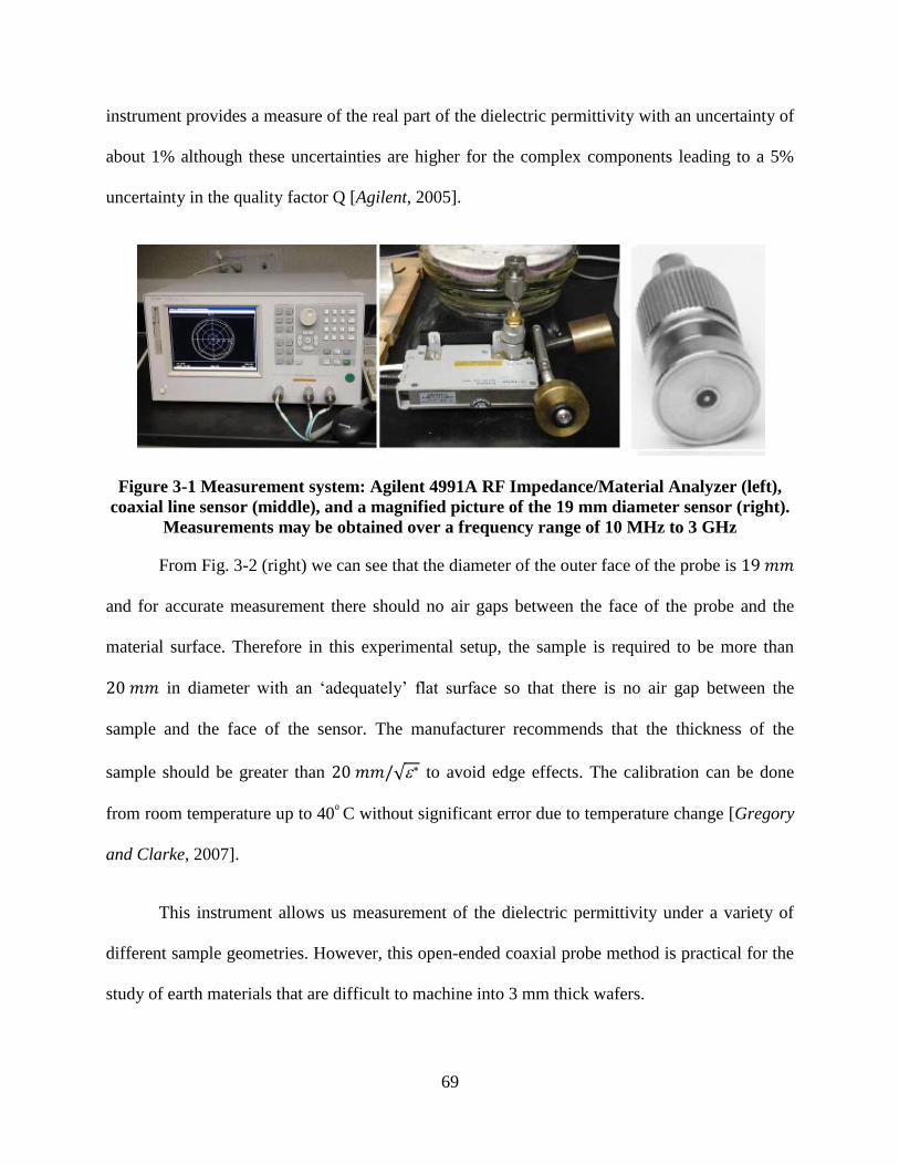
3.1 Measurement System ..................................................................................................... 68
3.2 RF I-V Technique........................................................................................................... 70
3.2.1 Calibration............................................................................................................... 73
Page 7
vii
3.2.2 Advantages and Limitations of the RF IV Method ................................................. 76
3.3 Cold Compression Technique ........................................................................................ 76
3.3.1 Advantages and Limitations of the Cold Compression Technique ........................ 79
3.4 Material Characterization ............................................................................................... 79
3.4.1 Scanning Electron Microscope (SEM) ................................................................... 80
3.4.2 Helium Pycnometer ................................................................................................ 81
3.4.3 Mercury Porosimeter .............................................................................................. 82
3.4.4 X-ray Diffraction (XRD) ........................................................................................ 84
3.4.5 X-ray Fluorescence (XRF) Elemental Analysis ..................................................... 84
3.5 Summary ........................................................................................................................ 85
CHAPTER 4. MEASUREMENTS ON MINERALS AND SYNTHETIC SAMPLES ........ 86
4.1 Introduction .................................................................................................................... 86
4.2 Single Crystal Measurements ......................................................................................... 86
4.3 Measurement on cold compressed halite and sylvite samples ....................................... 91
4.4 Salt With Glass Beads .................................................................................................... 95
4.5 Mixing Model ................................................................................................................. 98
4.5.1 Inclusion of lower permittivity than the matrix ...................................................... 98
4.5.2 Inclusion of higher permittivity than the matrix ................................................... 102
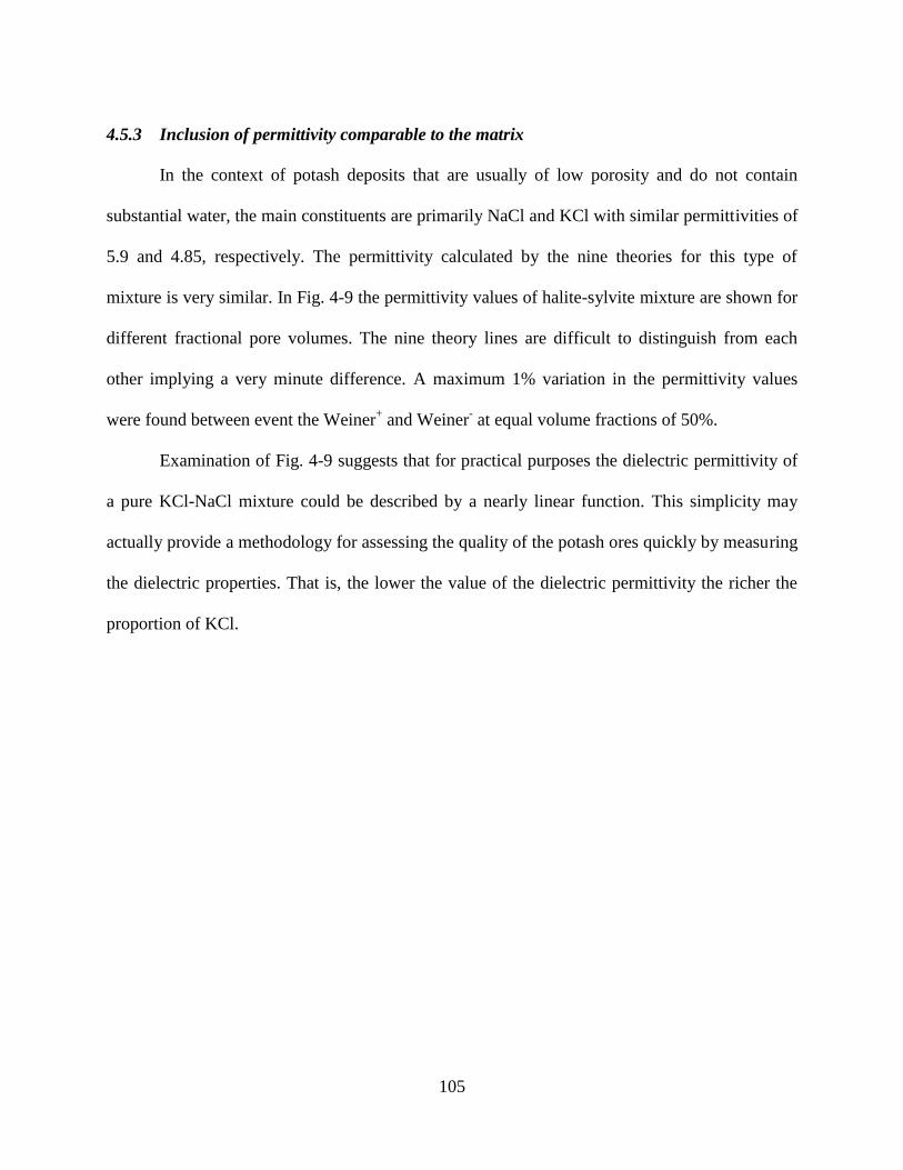
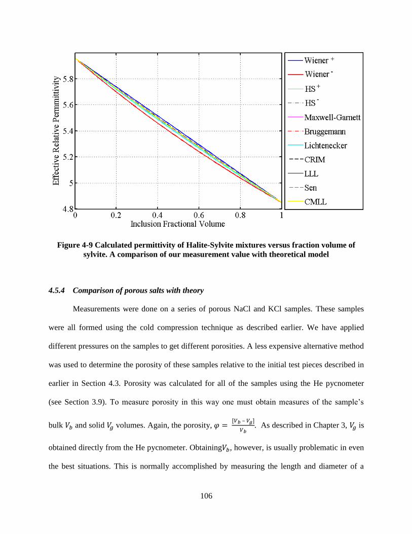
4.5.3 Inclusion of permittivity comparable to the matrix .............................................. 105
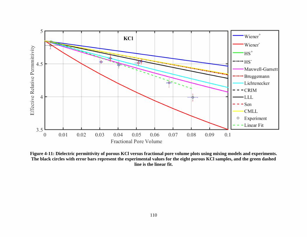
4.5.4 Comparison of porous salts with theory ............................................................... 106
Page 8
viii
4.6 Summary ...................................................................................................................... 113
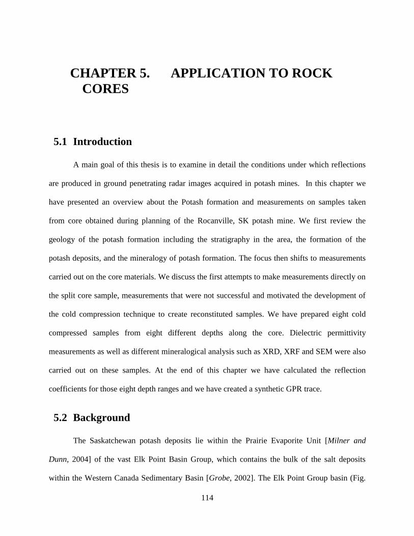
CHAPTER 5. APPLICATION TO ROCK CORES ............................................................. 114
5.1 Introduction .................................................................................................................. 114
5.2 Background .................................................................................................................. 114
5.2.1 Geology and Geophysical Logs at Rocanville ...................................................... 117
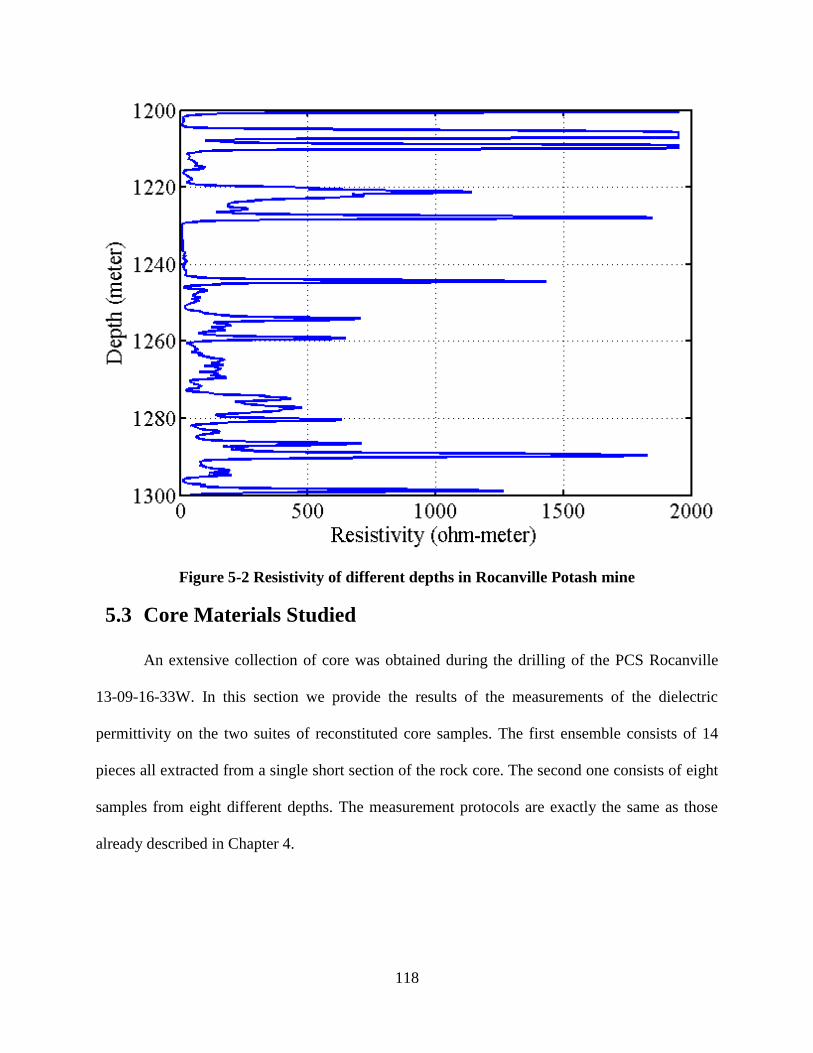
5.3 Core Materials Studied ................................................................................................. 118
5.3.1 Heterogeneity in a single sample .......................................................................... 119
5.3.2 Variations with depth ............................................................................................ 127
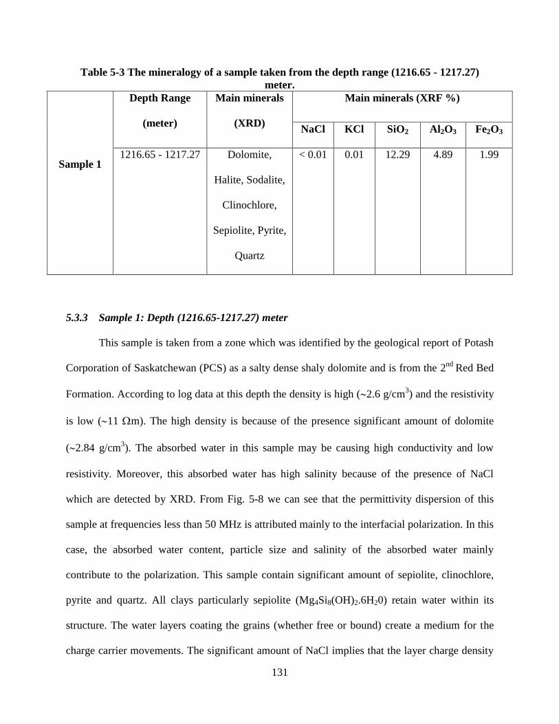
5.3.3 Sample 1: Depth (1216.65-1217.27) meter ........................................................... 131
5.3.4 Sample 2: Depth (1223.67-1224.30) meter ........................................................... 133
5.3.5 Sample 3: Depth (1230.28-1230.49) meter ........................................................... 134
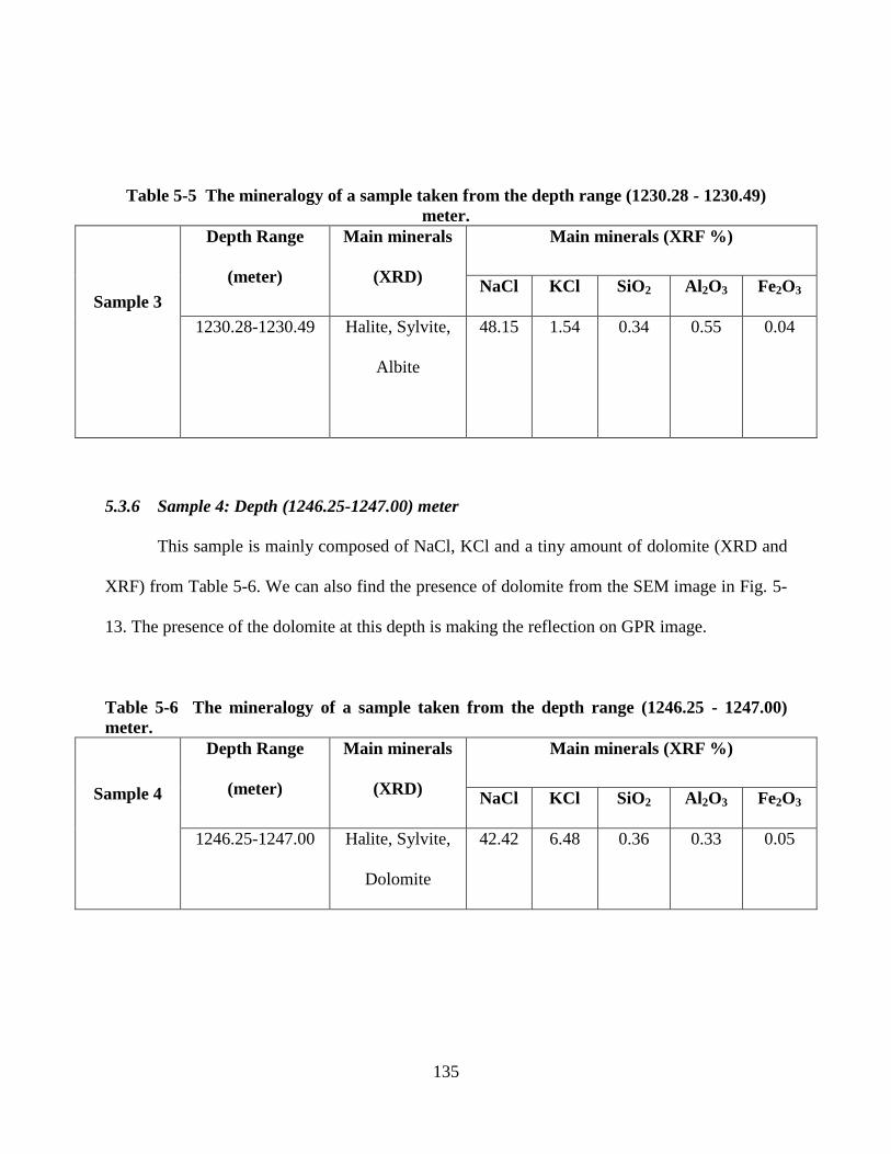
5.3.6 Sample 4: Depth (1246.25-1247.00) meter ........................................................... 135
5.3.7 Sample 5: Depth (1255.63-1256.31) meter ........................................................... 138
5.3.8 Sample 6: Depth (1266.34-1266.71) meter ........................................................... 140
5.3.9 Sample 7: Depth (1271.86-1272.49) meter ........................................................... 142
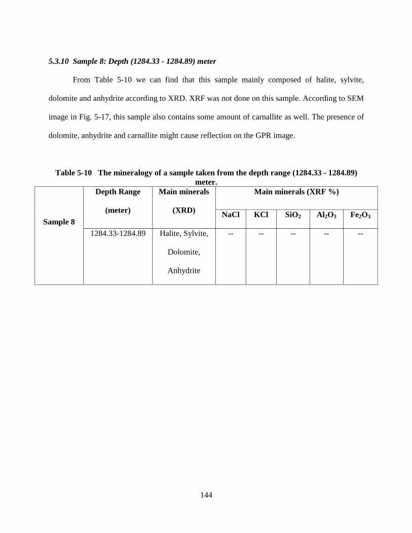
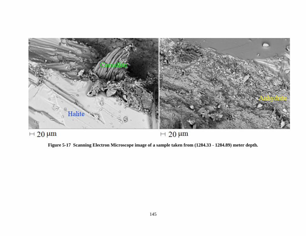
5.3.10 Sample 8: Depth (1284.33 - 1284.89) meter ......................................................... 144
5.3.11 Relatively conductive zone (e.g clay or clayey evaporite) ................................... 146
5.3.12 Brine inclusions effect .......................................................................................... 147
5.4 Reflection modelling .................................................................................................... 148
5.5 Summary ........................................................................................................................ 153
Page 9
ix
CHAPTER 6. CONCLUSION ............................................................................................. 154
6.1 Summary of Work Completed ..................................................................................... 154
6.2 Recommendation for Future Work .............................................................................. 156
References .................................................................................................................................. 158
Appendix A ................................................................................................................................. 166
Appendix B ................................................................................................................................. 180
Page 10
x
List of Figures
Figure 2-1 Parallel plate capacitor using DC circuit ..................................................................... 30
Figure 2-2 Parallel plate capacitor using AC circuit ..................................................................... 31
Figure 2-3 Reflected and transmitted signals for transverse electromagnetic wave (TEM). ........ 35
Figure 2-4 Loss tangent vector diagram. ...................................................................................... 38
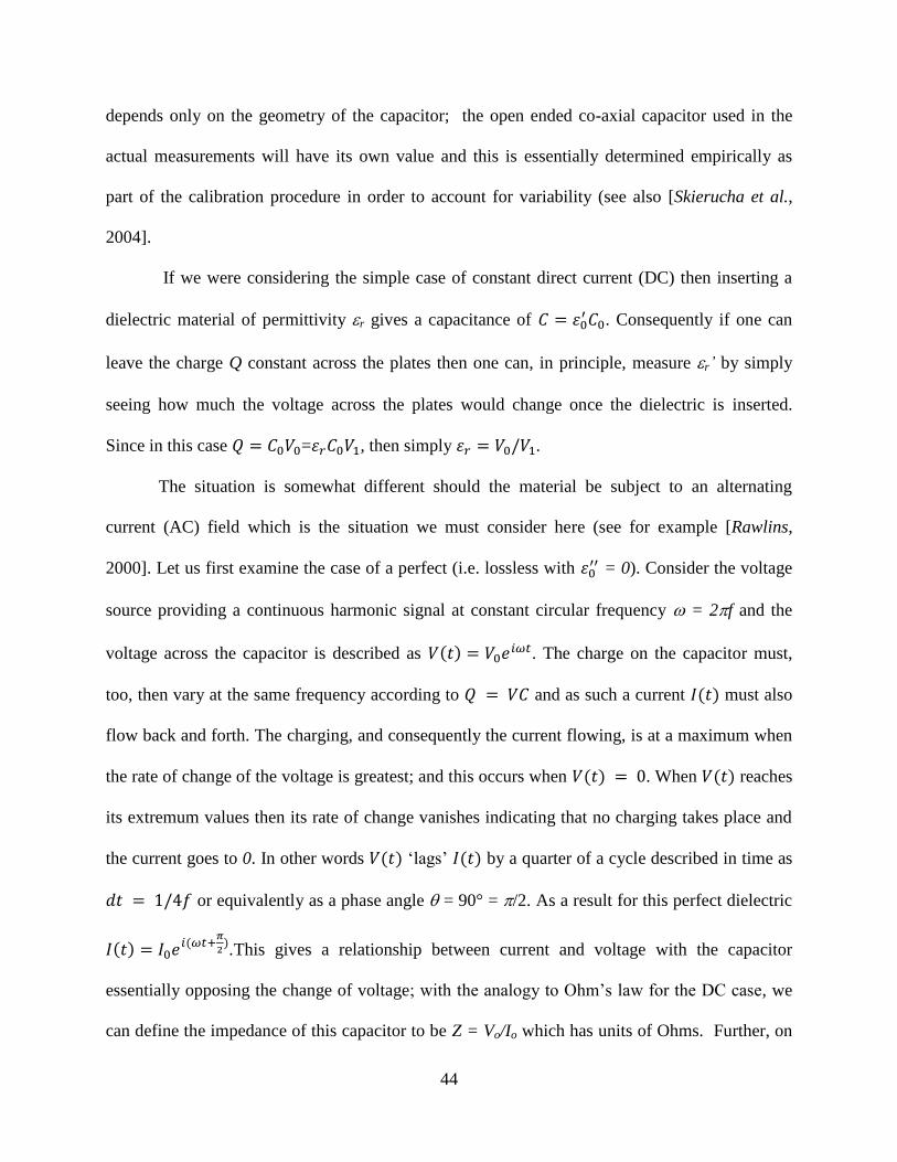
Figure 2-5 Essential components of an IV measurement system that includes an AC voltage
source, a voltmeter to provide V(t) shown in red in right graph and an ammeter to provide I(t)
shown in green in right graph. The sample is shown as being mounted in between two parallel
plates of capacitor in this example. For a perfect lossless dielectric dt = 1/4f equating to a phase
shift angle of /2. For a lossy case /2 and dt < 1/4f.
....................................................................................................................................................... 46
Figure 2-6 Different polarization processes occur at different frequencies causing dielectric
dispersion (Ref after (Agilent)). .................................................................................................... 47
Figure 2-7 Dipolar rotation in the electric field (Ref after (Agilent)). .......................................... 48
Figure 2-8 Electronic polarization of atoms. ................................................................................ 49
Figure 2-9 Atomic polarization between ions ............................................................................... 50
Figure 2-10 Change in polarization due to sudden change in applied electric field. .................... 53
Figure 2-11 Debye relaxation for water at 30 °C (ref after (Agilent)).......................................... 54
Figure 2-12 Cole-Cole representation of the Debye model of water at 300C. (ref. after (Agilent)).
....................................................................................................................................................... 55
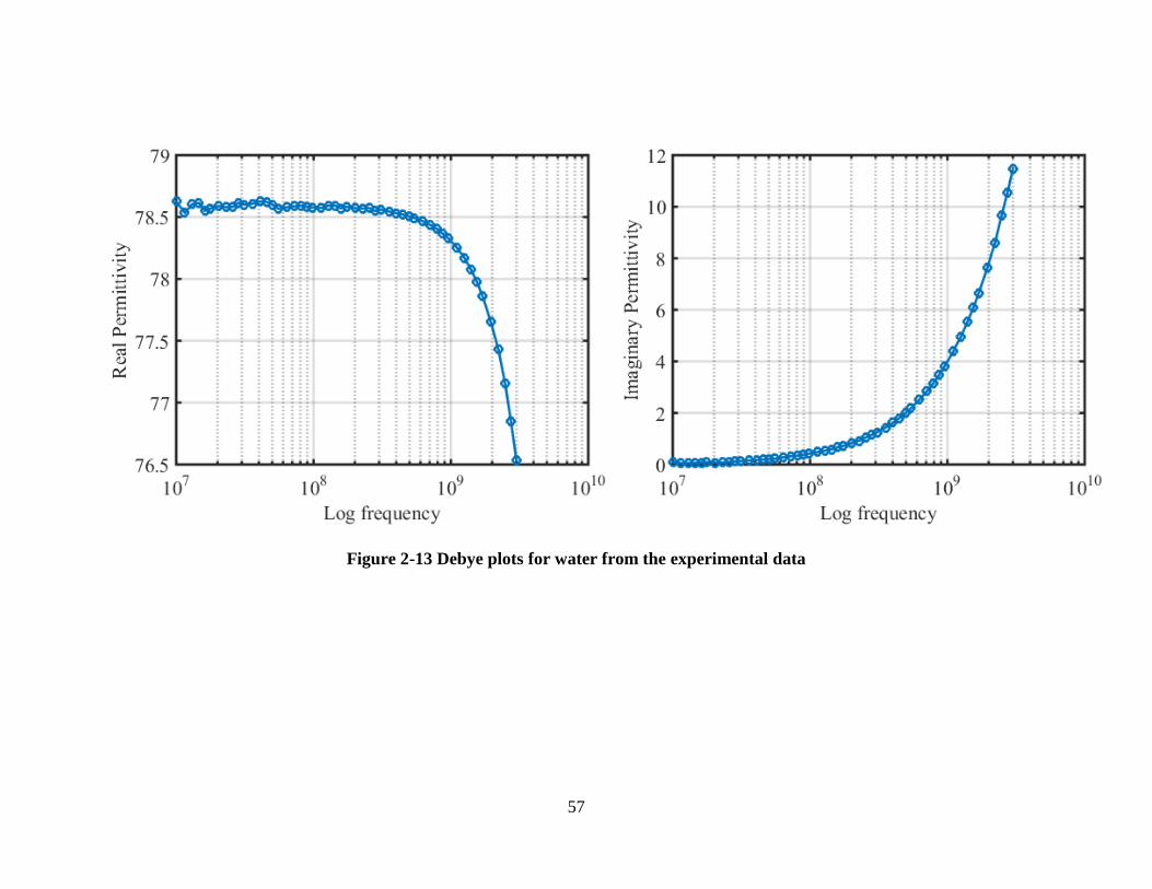
Figure 2-13 Debye plots for water from the experimental data .................................................... 57
Figure 2-14 Cole-Cole plot for water from the experimental data (left). Circle fit of the data is
also shown (right). ........................................................................................................................ 58
Figure 3-2 Coaxial probe (left) and a cross section of the sensor. The electric field lines fringe
from the end of the sensor into the sample under measurement. .................................................. 70
Page 11
xi
Figure 3-3 Basic principle of RF I-V technique and vector voltage ratio relationship (ref. after
Agilent). ........................................................................................................................................ 71
Figure 3-4 Vector voltage ratio relationship to impedance for E4991A. ..................................... 72
Figure 3-5 Dielectric permittivity of halite and sylvite single crystal to check the accuracy of
calibration of the equipment. ........................................................................................................ 75
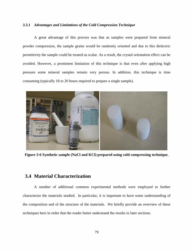
Figure 3-6 Synthetic sample (NaCl and KCl) prepared using cold compressing technique. ....... 79
Figure 3-7 Cumulative intrusion versus pressure for a porous NaCl sample (measured porosity
4%) using Hg porosimeter. ........................................................................................................... 83
Figure 4-1 Group of single evaporite crystals. A is halite and sylvite, B and C are calcite, D, E, F
and G are gypsum and H is dolomite. ........................................................................................... 90
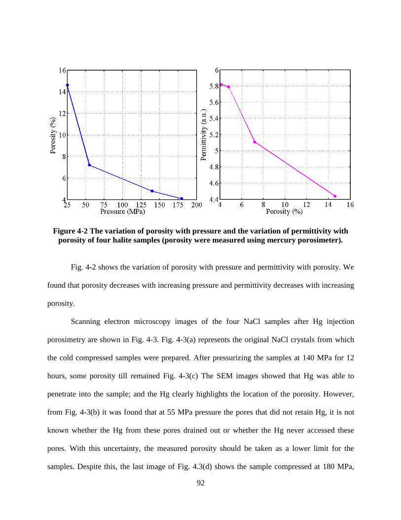
Figure 4-2 The variation of porosity with pressure and the variation of permittivity with porosity
of four halite samples (porosity were measured using mercury porosimeter). ............................. 92
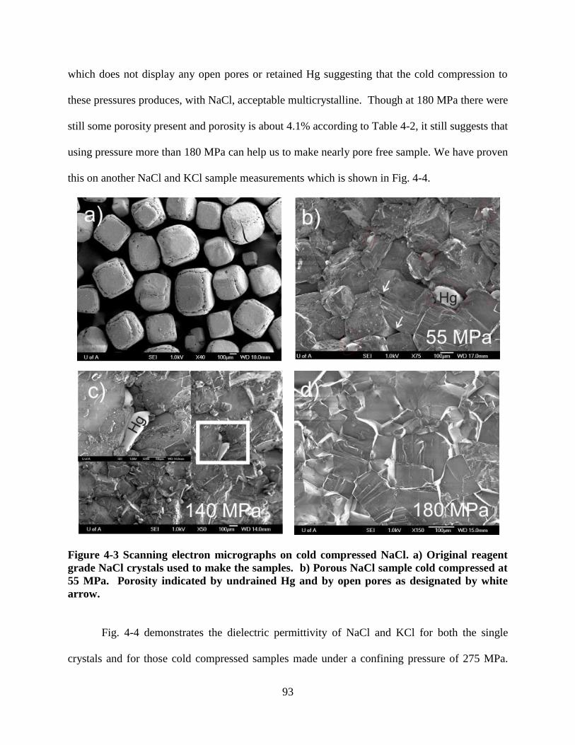
Figure 4-3 Scanning electron micrographs on cold compressed NaCl. a) Original reagent grade
NaCl crystals used to make the samples. b) Porous NaCl sample cold compressed at 55 MPa.
Porosity indicated by undrained Hg and by open pores as designated by white arrow. ............... 93
Figure 4-4 Dielectric permittivity of a) cold compressed KCl and single sylvite (KCl) crystal; b)
cold compressed NaCl and single halite (NaCl) crystal. Cold compressed samples showed
similar permittivity values as single crystal. ................................................................................. 94
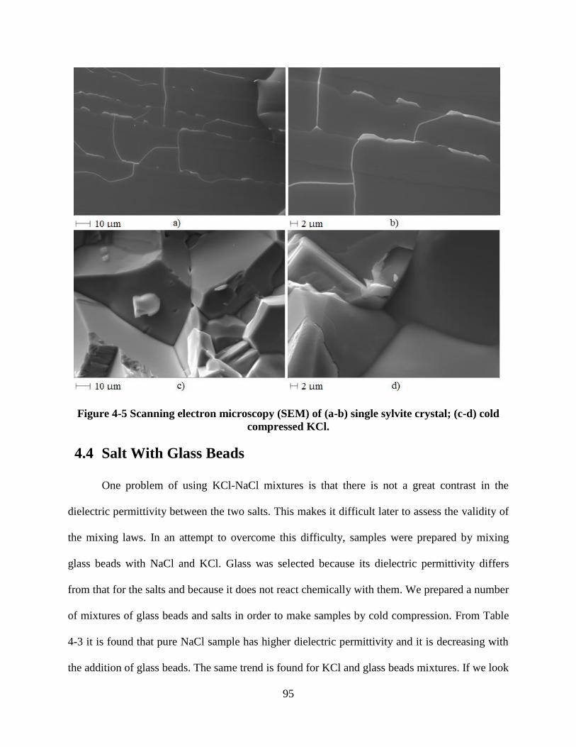
Figure 4-5 Scanning electron microscopy (SEM) ........................................................................ 95
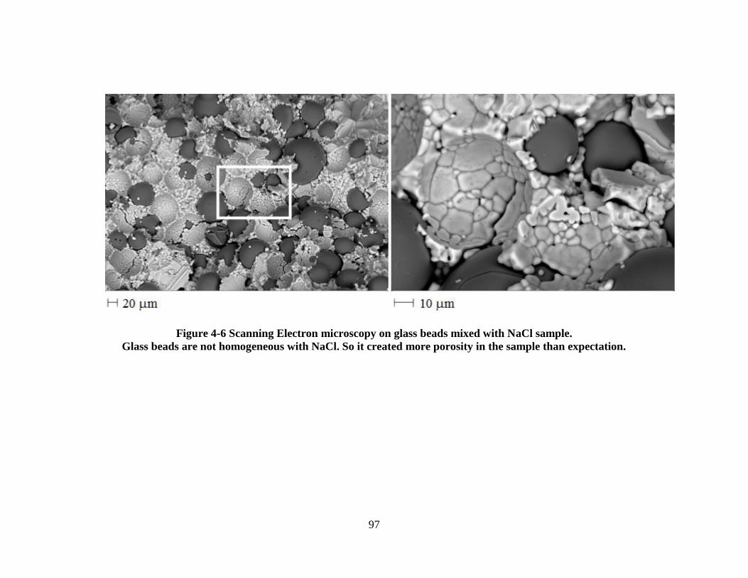
Figure 4-6 Scanning Electron microscopy on glass beads mixed with NaCl sample. .................. 97
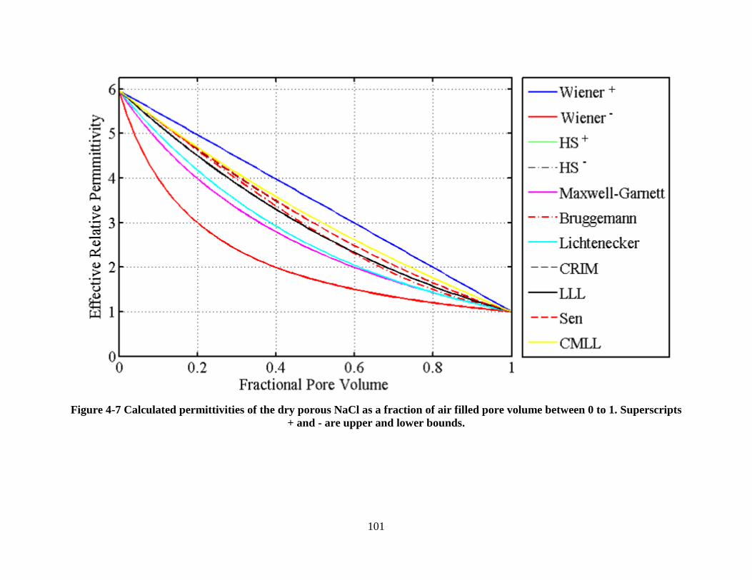
Figure 4-7 Calculated permittivities of the dry porous NaCl as a fraction of air filled pore volume
between 0 to 1. Superscripts + and - are upper and lower bounds. ............................................ 101
Page 12
xii
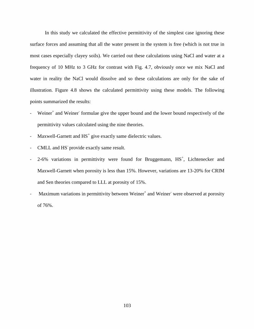
Figure 4-8 Calculated permittivity of the water saturated NaCl at fraction pore volume between
0 to 1. Permittivities were calculated from nine mixing theories. .............................................. 104
Figure 4-9 Calculated permittivity of Halite-Sylvite mixtures versus fraction volume of sylvite.
A comparison of our measurement value with theoretical model .............................................. 106
Figure 4-10: Dielectric permittivity of porous NaCl versus fractional pore volume plots using
mixing models and experiments. The black circles with error bars represent experimental values
for the eight porous NaCl samples, and the green dashed line is the linear fit. .......................... 109
Figure 4-11: Dielectric permittivity of porous KCl versus fractional pore volume plots using
mixing models and experiments. The black circles with error bars represent the experimental
values for the eight porous KCl samples, and the green dashed line is the linear fit. ................ 110
Figure 5-1: Potash mining belt (Reproduced with permission from NorthRim) ........................ 116
Figure 5-2 Resistivity of different depths in Rocanville Potash mine ........................................ 118
Figure 5-3 A piece of core sample in the depth range of 1238.678-1239.37 meter ................... 119
Figure 5-4 Real and imaginary permittivity versus frequency for raw potash samples ........... 123
Figure 5-5 Real and imaginary permittivity versus frequency for compressed potash samples 124
Figure 5-6 (a) represents dielectric values placing each of the 14 pieces of the core directly on
the sensor. The core was taken from depth (1238.68-1239.31 meter, (b). represents the dielectric
values of 14 (compressed) samples. All the permittivity values were averaged out from four
measurements. (c, d) represent the standard deviations (S.D.) of the permittivity in the raw and
compressed samples respectively. .............................................................................................. 126
Figure 5-7: Compressed samples at the eight different depths of Rocanville potash mine. ....... 128
Figure 5-8 The real and imaginary relative permittivity of samples taken from GPR reflection
zone. The samples names stand for the depth it was taken from. ............................................... 129
Page 13
xiii
Figure 5-9 Calculated speed wave for the samples taken from GPR reflection zone. The name of
the samples stand for the depth it was taken from. At high clay content the velocity becomes a
function of frequency. ................................................................................................................. 130
Figure 5-10 Scanning Electron Microscope image of a sample taken from (1216.65 - 1217.27)
meter depth.................................................................................................................................. 132
Figure 5-11 Scanning Electron Microscope image of a sample taken from (1223.67-1224.30)
meter depth.................................................................................................................................. 134
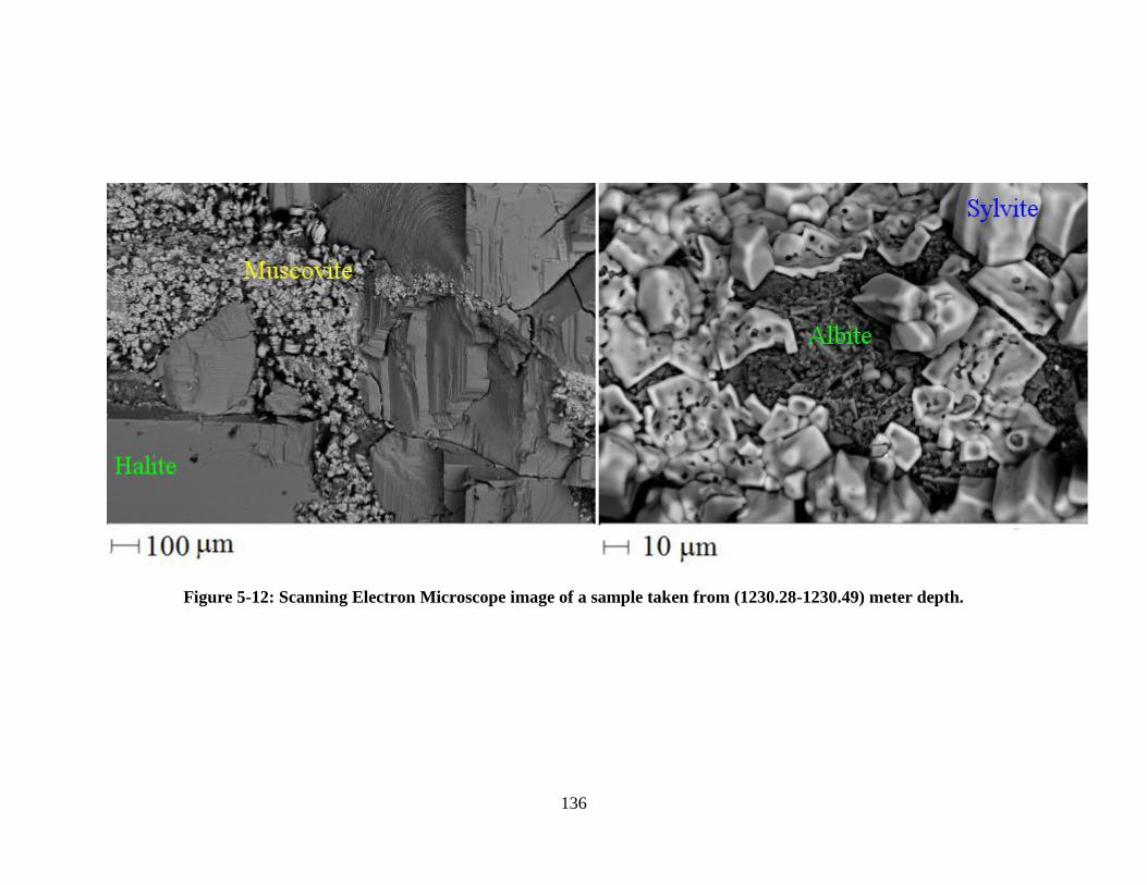
Figure 5-12: Scanning Electron Microscope image of a sample taken from (1230.28-1230.49)
meter depth.................................................................................................................................. 136
Figure 5-13 Scanning Electron Microscope image of a sample taken from (1246.25-1247.00)
meter depth.................................................................................................................................. 137
Figure 5-14 Scanning Electron Microscope image of a sample taken from (1255.63 - 1256.31)
meter depth.................................................................................................................................. 139
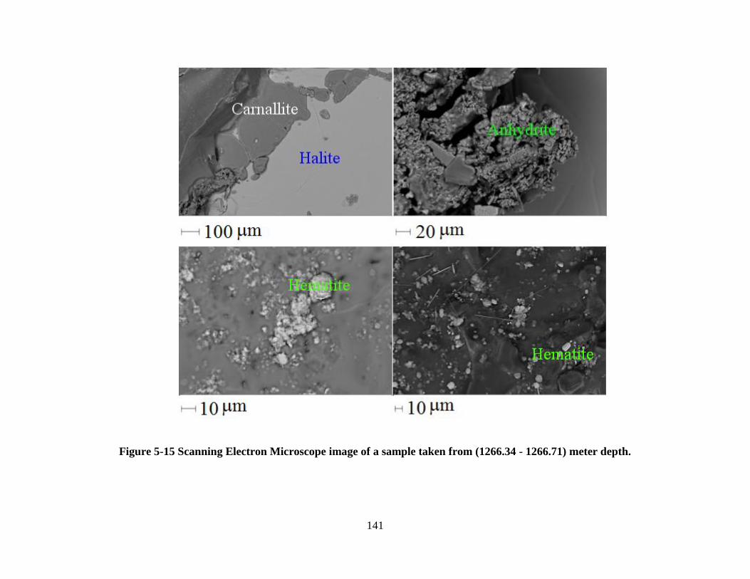
Figure 5-15 Scanning Electron Microscope image of a sample taken from (1266.34 - 1266.71)
meter depth.................................................................................................................................. 141
Figure 5-16 Scanning Electron Microscope image of a sample taken from (1271.86 - 1272.49)
meter depth.................................................................................................................................. 143
Figure 5-17 Scanning Electron Microscope image of a sample taken from (1284.33 - 1284.89)
meter depth.................................................................................................................................. 145
Figure 5-18 Change of reflection coefficient with frequency. .................................................... 150
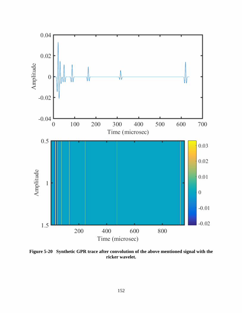
Figure 5-20 Synthetic GPR trace after convolution of the above mentioned signal with the
ricker wavelet. ............................................................................................................................. 152
Page 14
xiv
List of Tables
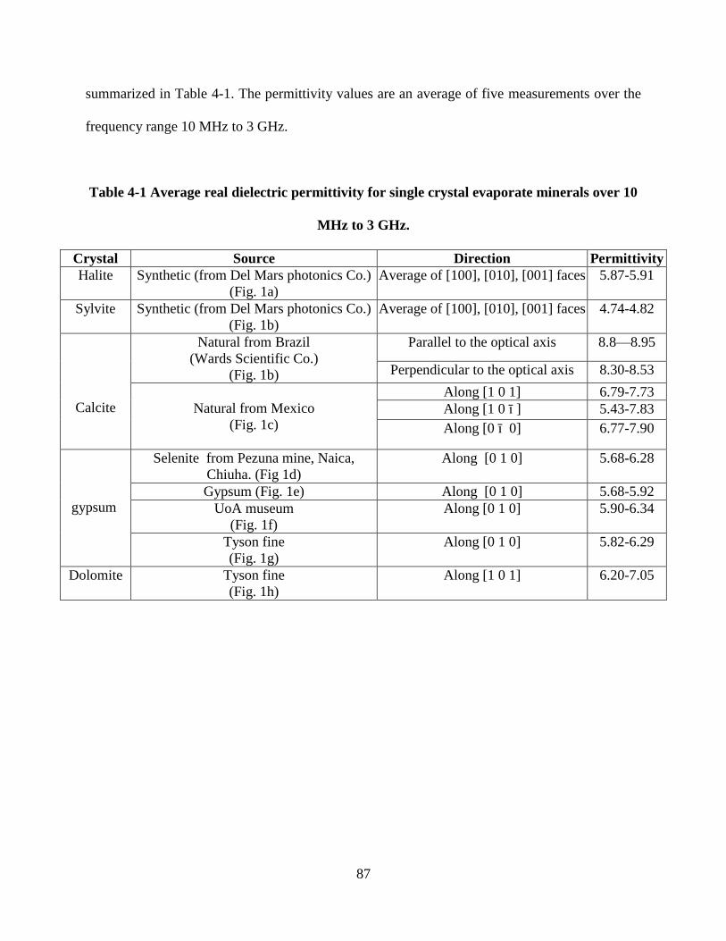
Table 4-1 Average real dielectric permittivity for single crystal evaporate minerals over 10 MHz
to 3 GHz. ....................................................................................................................................... 87
Page 15
xv
Table 4-2 Dielectric permittivity and porosity values for synthetic NaCl samples compressed at
different pressure. Porosity values using mercury porosimeter. ................................................... 91
Table 4-3 Dielectric permittivity of glass beads mixed with KCl and NaCl according to mass
percentage. .................................................................................................................................... 96
Table 4-4 Dielectric permittivity, porosity, grain volume and bulk volume of NaCl and KCl
samples. Both the grain volume and bulk volume were calculated using He pycnometer. ........ 108
Table 4-5: Relative percentage change between the experimental results and mixing theories for
NaCl samples. Variance and standard deviation is also shown. Experimental values are taken as
reference. ..................................................................................................................................... 111
Table 4-6 Relative percentage change between the experimental results and mixing theories for
KCl samples. Variance and standard deviation is also shown. Experimental values are taken as
reference. ..................................................................................................................................... 112
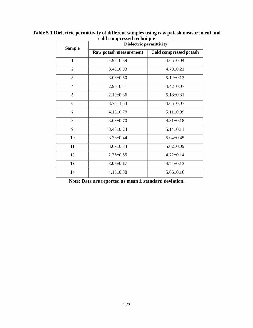
Table 5-1 Dielectric permittivity of different samples using raw potash measurement and cold
compressed technique ................................................................................................................. 122
Table 5-2 Dielectric permittivity (real and imaginary) and velocity in different depth ranges.
Data reported as mean ± standard deviation. The measurement frequency was 10 MHz to 3 GHz
..................................................................................................................................................... 128
Table 5-3 The mineralogy of a sample taken from the depth range (1216.65 - 1217.27) meter. 131
Table 5-4 The mineralogy of a sample taken from the depth range (1223.67 - 1224.30) meter.
..................................................................................................................................................... 133
Table 5-5 The mineralogy of a sample taken from the depth range (1230.28 - 1230.49) meter.
..................................................................................................................................................... 135
Page 16
xvi
Table 5-6 The mineralogy of a sample taken from the depth range (1246.25 - 1247.00) meter.
..................................................................................................................................................... 135
Table 5-7 The mineralogy of a sample taken from the depth range (1255.63 - 1256.31) meter.
..................................................................................................................................................... 138
Table 5-8 The mineralogy of a sample taken from the depth range (1266.34 - 1266.71) meter.
..................................................................................................................................................... 140
Table 5-9 The mineralogy of a sample taken from the depth range (1271.86 - 1272.49) meter.
..................................................................................................................................................... 142
Table 5-10 The mineralogy of a sample taken from the depth range (1284.33 - 1284.89) meter.
..................................................................................................................................................... 144
Table 5-11 Resistivities of GPR reflection zones. ..................................................................... 147
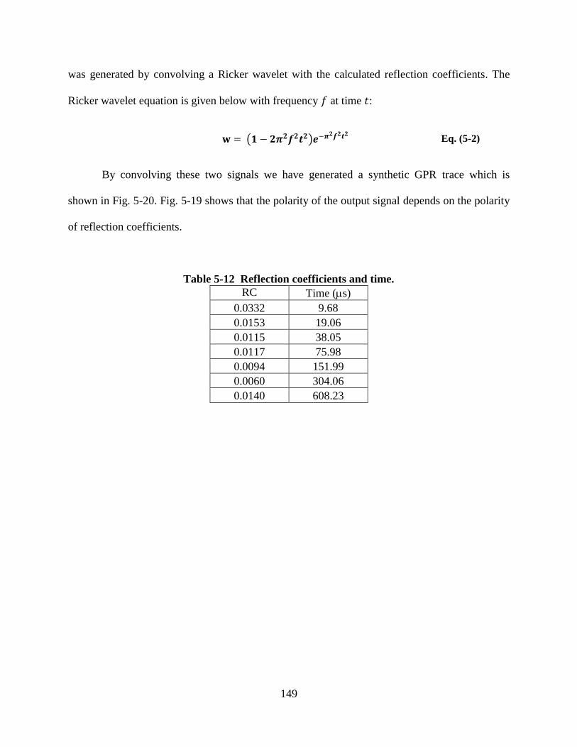
Table 5-12 Reflection coefficients and time. ............................................................................. 149
List of Symbols
Dielectric permittivity
Page 17
xvii
Relative permittivity
Free space permittivity
Real dielectric permittivity or dielectric storage
Imaginary dielectric permittivity or dielectric loss
Complex dielectric permittivity
Relative equivalent dielectric permittivity
Conductivity
Effective conductivity
Angular frequency
Capacitance with dielectric material between plates
Capacitance without dielectric material between plates
A Area of the capacitor plates
d Distance between plates
V Voltage
Charging current
Loss current
Conductance
Frequency
Electric displacement (electric flux density)
Electric field
Electric displacement vector
Magnetic field intensity
Electric charge density
Page 18
xviii
Electric current density vector
Magnetic permeability
Magnetic permeability of free space
Relative magnetic permeability
Total induced magnetization
Magnetic hysteresis loss
Dielectric constant
Refractive index
Intrinsic wave impedance
Speed of light
Volume magnetic susceptibility
tan Ratio of the imaginary part of the dielectric constant to the real part.
Dissipation factor
Quality factor
Propagation phase velocity of an EM wave in any media
P Power dissipation
Z Intrinsic electromagnetic impedance of a material
R Plane wave reflection co-efficient
A Absorption coefficient
Relaxation frequency
Relaxation time
Relaxation frequency
Angle between the real axis and the high frequency intercept line
Page 19
xix
Complex dielectric permittivity of the background
Complex dielectric permittivity of the inclusions
Fractional volume of the background
Fractional volume of the inclusions
Q Quality factor
Zr Roll-off impedance
Initial pressure of the gas
Final pressures of the gas
Initial volume
Final volume
Volume of the reference cell
Volume of the cell containing the sample
Volume of the solid portion of the sample
Porosity
Bulk volume
Diameter of pore throat
Applied pressure
Surface tension of mercury
Contact angle
Sylvite
Halite
Carnallite
Muscovite
Page 20
xx
Dolomite
Anhydrite
Gypsum
Calcite
List of Acronyms
Page 21
xxi
GPR Ground Penetrating Radar
EM Electromagnetic
TDR Time domain reflectometry
MPa Mega Pascal
SEM Scanning Electron Microscopy
XRD X-Ray diffraction
XRF X-Ray fluorescence
DC Direct current
AC Alternating current
TEM Transverse electromagnetic
FDR Frequency domain reflectometry
RF-IV Radiofrequency - Current Voltage
BHS Bruggeman-Hanai-Sen
CRIM Complex refractive index mixture
LLL Landau, Lifshitz, Looyenga
HS+ Hashin-Strickmann upper limit
HS- Hashin-Strickmann lower limit
SNR Signal-to-noise ratio
IR Infrared
PCS Potash Corp. of Saskatchewan
Page 22
22
CHAPTER 1. INTRODUCTION
This work is mainly focused on the dielectric property measurements of geological
materials from potash mines in Saskatchewan. It is motivated to support the interpretation of
Ground Penetrating Radar (GPR) surveys conducted in the potash mines. In this first chapter, we
simply explain the motivations for the work and provide a brief outline of the contents of the
following chapters.
1.1 Background
Dielectric permittivity ( ) is an important physical property that is widely used in various
realms of science including geophysics, condensed matter physics, biology, forestry, agriculture,
engineering and hydrology [Topp et al., 1980]. One of the most important uses of dielectric
constant is to quantify water content [Josh et al., 2012]. Measurements of are used as a proxy
for water content in soils through empirical relationships [e.g., Malicki et al., 1996; Roth et al.,
1992; Topp et al., 1980]. Further, using GPR the structure of the near surface of the Earth may be
imaged at radio frequencies (~10 MHz to 1.5 GHz). Water is highly influential on such wave
propagation over this frequency range because its relative dielectric permittivity is nearly 80
while that of the minerals forming the rocks ranges from about 3 to 9 and for air for all practical
purposes can be taken to be 1 [Weast, 1984]. As such, even small amounts of water within the
pore space of a rock can strongly influence the propagation of GPR signals.
Both invasive (time domain reflectometry and cross borehole radar) and non-invasive
(ground penetrating radar) electromagnetic techniques are used to estimate water content and
porosity [Sakaki et al., 1998; Sen et al., 1981]. This is because the propagation speed of
Page 23
23
electromagnetic (EM) radiation through such materials is governed by the bulk or effective
dielectric permittivity that depends strongly on water content. Therefore the knowledge of
dielectric permittivity is crucial to the accurate interpretation of GPR images. The soil science
literature mostly focuses on moisture estimation primarily using time domain reflectometry
techniques (TDR); the literature associated with this topic large and relatively mature [Robinson
et al., 2003]. In contrast, studies of the relationships between GPR wave propagation and the
material physical properties are not as advanced. This is likely due to the broader range of
geological topics encountered in GPR studies. As well, actually obtaining reliable values of
applicable to lower porosity materials that do not necessarily contain water is difficult.
Non-destructive GPR or geo-radar has wide application in hydrology, sedimentology,
geological structure, fractures, glaciers and land mine detection. Moreover, it is a popular
technique for imaging the subsurface and is particularly useful in electrically resistive materials
such as clean sands, crystalline igneous and metamorphic rock, salt deposits, concrete, and ice
[Daniels et al., 1988]. Despite this, a lack of understanding of physical basis may result in the
unsuccessful interpretation of GPR data. Different earth materials have different dielectric
permittivities, wave speeds, and attenuations which lead to a reflection of the EM waves at the
interfaces between these materials. Finding out the reasons causing reflection on GPR image
helps us to interpret GPR data more precisely.
The overriding motivation for this work was the need to better understand GPR
observations within potash formations in Saskatchewan. Potash is primarily used as an
agricultural fertilizer. Potash ore is mainly composed of sylvite ( ) which is an important
industrial chemical. The richest sylvite bearing potash contains substantial proportions of other
evaporate minerals particularly halite ( ) and some carnallite . Moreover,
Page 24
24
formations adjacent to the best ores contain a wide variety of additional evaporates such as
anhydrite, gypsum, calcite, and dolomite depending upon the depositional and burial history.
GPR has been widely used in salt and potash formations [Annan et al., 1988; Chiba et al.,
2006; Gorham et al., 2002; Holser et al., 1972; Igel et al., 2006; Kulenkampff and Yaramanci,
1993; Thierbac, 1974; Unterberger, 1978] to provide detailed structural information that helps
the development of underground workings for mining, hazardous waste storage, and scientific
studies. Moreover GPR is employed in a nearly real time basis to assist the steering of large
mining machines. Indeed, excavator operators in potash mines direct their machines by
monitoring their position within the ore zone on the basis of known reflections.
In the Saskatchewan potash mines, high quality ore zones are often bounded by thin
‘shale’ layers that are principally contaminated with anhydrite and calcite. The proximity of the
actual mine workings to such ‘shales’ is quite important must be considered during mining as
these layers act as weak zones that can easily part and cause roof failures. A photograph of such
a weak ‘shale’ layer is shown in Fig. 1-1.
Ground penetrating radars (GPR) attached to mining machines are often used to track
these shale layers so that the mine works will stay sufficiently away from them. As such, in order
to best interpret the underground observations it is important to understand the reflections seen;
but to do this fully requires appropriate knowledge of the physical properties of the constituent
evaporate minerals.
Page 25
25
Figure 1-1 Different layers in a Potash mine. The grey colored layers are showing the presence of shale.
Page 26
26
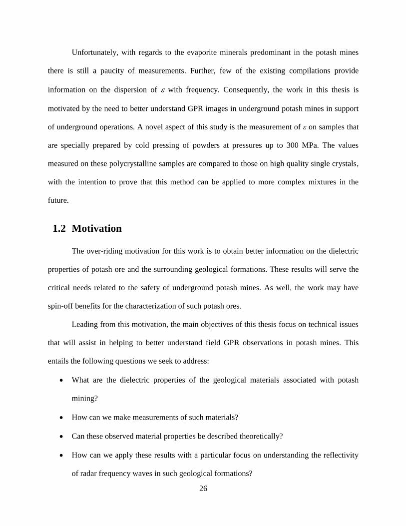
Unfortunately, with regards to the evaporite minerals predominant in the potash mines
there is still a paucity of measurements. Further, few of the existing compilations provide
information on the dispersion of with frequency. Consequently, the work in this thesis is
motivated by the need to better understand GPR images in underground potash mines in support
of underground operations. A novel aspect of this study is the measurement of ε on samples that
are specially prepared by cold pressing of powders at pressures up to 300 MPa. The values
measured on these polycrystalline samples are compared to those on high quality single crystals,
with the intention to prove that this method can be applied to more complex mixtures in the
future.
1.2 Motivation
The over-riding motivation for this work is to obtain better information on the dielectric
properties of potash ore and the surrounding geological formations. These results will serve the
critical needs related to the safety of underground potash mines. As well, the work may have
spin-off benefits for the characterization of such potash ores.
Leading from this motivation, the main objectives of this thesis focus on technical issues
that will assist in helping to better understand field GPR observations in potash mines. This
entails the following questions we seek to address:
What are the dielectric properties of the geological materials associated with potash
mining?
How can we make measurements of such materials?
Can these observed material properties be described theoretically?
How can we apply these results with a particular focus on understanding the reflectivity
of radar frequency waves in such geological formations?
Page 27
27
1.3 Chapter Description
In this thesis I present dielectric measurements on rock minerals from the potash mines.
Dielectric measurements were done on single crystals, on cold-compressed synthetic samples of
the minerals associated with the potash deposits, and on natural and cold compressed potash
samples. This thesis has been organized into 6 chapters. In this chapter 1, the importance of
dielectric measurements and the motivation of this work were briefly discussed.
In chapter 2, I review the related theoretical background. This chapter provides
descriptions of dielectrics, Electromagnetic Wave (EM) propagation, and the techniques used to
measure dielectric properties. This chapter concludes with a review of the various effective
medium mixing theories that can be applied to predict the bulk dielectric properties given the
relative proportions of the chemical constituents.
Chapter 3 provides a detailed overview of the experimental set up and the laboratory
procedures that I used for the measurements. A key part of this chapter focuses on issues related
to sample preparation; and the strategy of cold-compressing pellets of fine powders under high
pressures is described. The concluding sections of this chapter describe the different techniques
utilized to properly characterize the samples. Chapter 4 includes the results of the dielectric
measurements on high quality single crystals, followed by those on the various cold compressed
synthetic samples. This chapter concludes with a comparison of the observations to the mixing
theory models.
Chapter 5 is mainly focused on the measurements samples taken from an actual potash
core. The chapter begins with a brief review of the geology of the region. Dielectric
measurements on cold-compressed samples taken from various depths along the core are then
described. These samples were carefully characterized using Scanning Electron Microscopy
Page 28
28
(SEM) to understand the material structure, X-Ray diffraction (XRD) to know the mineralogical
constituents, and X-Ray fluorescence (XRF) to gain some understanding of the overall chemical
composition and mineralogy. Finally, these laboratory measurements were then employed to
create a synthetic GPR traces.
The concluding Chapter 6 reviews the results of the measurements and judges the quality
of the sample preparation methodologies. This chapter ends with a discussion of directions for
future work. Moreover, appendix A contains Cole-Cole plots for different samples and appendix
B reports MATLAB codes for mixing theories and reflection modeling.
Page 29
29
CHAPTER 2. BACKGROUND
2.1 Introduction
Having a clear idea about the physics of electromagnetic wave (EM) propagation is
necessary for the proper interpretation of ground penetrating radar (GPR) data. Such data
includes information on both the speeds of wave propagation as well as the relative differences
(through the strength of GPR reflections) of the dielectric properties between different layers. In
this Chapter, I discuss basic electromagnetic wave propagation theory. This is followed by a
review of effective medium mixing theory that may be used to help interpret the observations.
2.2 Dielectric Materials
Most earth materials are considered to be dielectrics. A material is generally considered
to be a dielectric if it satisfies the condition
, where is electrical conductivity
(Siemens/m), is angular frequency (rads/s), and is the dielectric permittivity (F/m) [Baker et
al., 2007]. If material stores energy in presence of an external electric field the material is called
as dielectric and the storage capacity of that material is named as dielectric permittivity.
Most readers will have seen dielectrics introduced in basic Physics discussions of the
parallel plate capacitor. If a charge is applied to two parallel plates the resulting device is known
as parallel plate capacitor. Fig. 2-1 shows the arrangement where a DC voltage is placed across a
parallel plate capacitor inducing positive and negative charges on the two plates. If a dielectric
material is placed between the plates, the capacitor can store more charge than if there is no
material (a vacuum). The capacitance of the parallel plate capacitor is enhanced due to the
Page 30
30
insertion of the dielectric materials. Moreover, an electric field opposing the field of the charged
plates is produced which results the reduction of the effective electric field. The capacitance of
the parallel plate capacitor is inversely related to the electric field between the plates.
Figure 2-1 Parallel plate capacitor using DC circuit
From Fig. 2-1, we can write
Eq. ( 2-1)
Eq. ( 2-2)
Eq. ( 2-3)
In Eq. (2-1 to 2-3), and are the capacitance with and without dielectric,
represents the real dielectric permittivity or sometimes dielectric constant (when imaginary part
of permittivity is very low compared to real part), A is the area of the capacitor plates and d is the
distance between them. From Eq. (2-3), we can find that the capacitance of a dielectric material
is related to the dielectric constant.
Fig. 2-2 shows parallel plate capacitor arrangement in an alternating current (AC) case
where an AC sinusoidal voltage source V is placed across the capacitor. The resulting current in
Page 31
31
this case will be made up of two type of current, one of them are charging current ( ) and the
other one is loss current ( ). Both the currents are related to the dielectric constant which can be
expressed as follows:
Eq. ( 2-4)
where
If then
Eq. ( 2-5)
Where, R = resistance and G is conductance of the parallel plate capacitor which
indicates the losses in the material.
Figure 2-2 Parallel plate capacitor using AC circuit
The complex dielectric constant consists of a real part which represents the storage and an
imaginary part which represents the loss. The following notations are used for the complex
dielectric constant interchangeably
Eq. ( 2-6)
According to electromagnetic theory, the electric displacement (electric flux density) is
described by the following equation
Page 32
32
Eq. ( 2-7)
where is the absolute permittivity (or permittivity),
Here represents the relative permittivity,
F/m is the free space permittivity
and is the electric field.
2.3 Maxwell's Equations
Better understanding of GPR behavior depends on the understanding of Maxwell’s
equations as they describe the relationship between material electromagnetic properties and EM
wave propagation as follows:
Eq. ( 2-8a)
Eq. (2.8b)
Eq. (2.8c)
Eq. (2.8d)
where is the electric field strength vector, is the magnetic flux density vector, is the
electric displacement vector, is the magnetic field intensity, is the electric charge density,
and is the electric current density vector. A good reference to understand the different notations
can be found in Schey [Schey and Schey, 2005].
From Maxwell’s equations we know electric currents generate magnetic fields and vice
versa. In order to understand GPR wave propagation (as discussed later in the EM wave
Page 33
33
Propagation section), it is imperative that the electric and magnetic physical properties are
understood.
GPR wave propagation primarily depends on the relative permittivity ( ), the magnetic
permeability ( ), and the electrical conductivity ( ). The relationship between relative
permittivity and magnetic permeability to the dielectric constant and refractive index are as
follows [Griffiths, 2012].
Eq. ( 2-9)
Eq. ( 2-10)
where:
dielectric constant which is dimensionless
refractive index which is dimensionless
permittivity (Farads per meter, F/m)
permittivity of free space ( F/m)
= relative permittivity (dimensionless)
μ = magnetic permeability (henries per meter, H/m)
= magnetic permeability of free space ( H/m)
= relative magnetic permeability , dimensionless.
Now we will discuss about the important parameters and their importance in
electromagnetic wave propagation or GPR wave propagation.
Page 34
34
2.4 Electromagnetic Wave propagation
It is essential to know the basics of electromagnetic (EM) wave propagation through
materials. Both electric and magnetic field appear together in a time-varying case is sinusoidal in
nature. This EM wave can propagate through free space at the speed of light or through materials
at slower speed.
A transverse electromagnetic wave (TEM) travels in free space consists of alternating and
in phase vector electric (V/m) and magnetic (A/m) fields that are both perpendicular to each
other and to the propagation direction. The wave moves at the speed of light c = 299792458 m/s
[Mohr et al., 2008] in vacuum. The ratio of the magnitudes
has real value equal to the
intrinsic wave impedance (in Ω).
Eq. ( 2-11)
where (8.854 187 817 ×10−12
Farad m-1
) and (4 X 10
-7 Henry m
-1) are the electrical
permittivity and the magnetic permeability of free space with
respectively.
Electromagnetic waves of various wavelengths exist. The wavelength of a signal is
inversely proportional to its frequency f ( ) which means that the wavelength decreases
with an increase in frequency and vice-versa. We will refer to the wavelength in free space aso.
Let us consider the optical view of dielectric behavior. Here we assume a flat slab of
material in space. When a TEM wave is incident on its surface both reflected and transmitted
waves are created (Fig. 2-3). In this case, the reflected wave is a consequence of the mismatch in
the impedances between free space Zo and the material Z (<Zo). A second portion of the
remaining wave energy is transmitted through the material. Since the wave velocity V in the slab
Page 35
35
is slower than the speed of light c in free space, the wavelength of the transmitted light is
shorter than o in free space and we can write the following Equations.
Z =
Eq. ( 2-12)
= Z0 =
= 120 Eq. ( 2-13)
=
Eq. ( 2-14)
V =
Eq. ( 2-15)
Since the material will always have some loss, there will be attenuation or insertion loss. For
simplicity the mismatch on the second border is not considered in Fig. 2-3.
Figure 2-3 Reflected and transmitted signals for transverse electromagnetic wave (TEM).
2.5 Electromagnetic Wave propagation
A given medium is electromagnetically characterized by three physical properties: the
magnetic permeability , the DC electrical conductivity , and the dielectric permittivity . All
of these properties are frequency dependent and behave differently with various frequency
ranges.
2.5.1 Magnetic Permeability
The magnetic permeability quantifies the capacity of a material to induce a magnetic
field within itself when it is inserted into an external magnetic field . That is, when a
Page 36
36
material is subjected to an induced magnetic field, magnetic permeability measures the magnetic
field energy stored and dissipated in that material [Powers, 1997]. The unit of permeability is the
Henry/m (H/m) which is also equivalent to Newtons/Ampere squared (N/A2). Permeability
relates the magnetic flux density (in Wb/m
2) to the magnetic field intensity (in
A/m) via . The relative magnetic permeability * may also be complex:
Eq. ( 2-16)
where the real and imaginary components describe the total induced magnetization (energy
storage) and the magnetic hysteresis loss (energy loss), respectively.
In geophysical investigations, it is more common to use the dimensionless volume
magnetic susceptibility
than the relative magnetic permeability. Some rocks
contain magnetic materials such as iron (ferrites), cobalt, nickel, and their alloys having
appreciable magnetic properties and it may become necessary to investigate permeability of
these rocks with regards to the propagation of EM waves [Mattei et al., 2007; Mattei et al., 2008;
Robinson et al., 1994; Van Dam et al., 2002]. However, most rocks, sediments and soils are only
weakly diamagnetic or paramagnetic with
< 10-4
and consequently the magnetic
permeability of most of minerals studied in this thesis can be ignored. Taking the permeability
equal to that of free space ( = 4 = ) suffices for most purposes [Ulaby et al., 2010].
Relative magnetic permeability is expressed by the following equation
=
Eq. ( 2-17)
Eq. ( 2-18)
Page 37
37
2.5.2 Electrical conductivity
Electrical conductivity describes how much electric current I exists under an applied
voltage V according to Ohm’s Law V = I/ [Saarenketo, 1998]. The conductivity is described in
units of Siemens/m (S/m) or, sometimes in the older literature, Mho/m. The reciprocal of is
the electrical resistivity given in Ohm-meter (-m). Electrical conductivity depends on
frequency but its behavior is relatively constant over the typical GPR frequency range of 25-
1,500 MHz [Martinez and Brynes, 2001]. Saline ground water and clay surfaces, for example,
contribute greatly to the overall conductivity of a given porous material inducing both wave
speed dispersion and enhanced attenuation of GPR signals [Cosenza et al., 2003].
2.5.3 Dielectric permittivity
Over the GPR frequencies studied here, the dielectric permittivity is the most
important parameter. It describes the polarization of induced or oriented electric dipoles within a
dielectric material. In general, the dielectric permittivity is complex and given by
Eq. ( 2-19)
where and are the real and the imaginary components, respectively. The real part , often
referred to as the dielectric constant despite the fact that it usually varies with frequency,
describes the ability of the material to store energy by polarization as a result of applying
electromagnetic radiation. The imaginary part describes the energy loss resulting from
dielectric hysteresis.
The real and imaginary components are 90° out of phase if we draw the complex
dielectric permittivity as a vector representation (Fig. 2-4). Their vector sum forms an angle
with the real axis ( ). The ratio of the energy lost to the energy stored indicates the relative
lossiness or loss factor of a material.
Page 38
38
Figure 2-4 Loss tangent vector diagram.
From Fig. 2-4 we can write
tan =
= D =
Eq. ( 2-20)
tan =
Eq. ( 2-21)
Here is defined as the ratio of the imaginary part of the dielectric constant to the real part
which is actually called the loss tangent. denotes dissipation factor and is quality factor. The
term “quality factor or -factor” is the reciprocal of the loss tangent. For very low loss materials,
since the loss tangent can be expressed in angle units of milliradians or microradians.
In the microwave region of the electromagnetic spectrum, the loss can be due to the
motion of conduction electrons/ions as well as by the dielectric hysteresis lag of dipole rotation
behind the rapidly fluctuating electric field. Therefore, the relative equivalent dielectric
permittivity can be written as
Eq. ( 2-22)
where is the angular frequency. This hysteresis yields heating of the material and is the
principle of microwave cooking and RF heating. Conversely, we can write the equivalent
conductivity
Eq. ( 2-23)
Page 39
39
These imply the dielectric loss increases with frequency while conductivity is an
important parameter at low frequencies. As mentioned earlier, the EM wave propagation speed is
equal to the speed of light c = ( o o)-1/2
in free space. Note the velocity of EM wave propagation
in Earth's atmosphere near sea level is around 0.3 m/ns but within typical earth materials it is
slower and usually between 0.05 and 0.15 m/ns [Baker et al., 2007; Daniels and Engineers,
2004]. This is because the dielectric permittivity of free space is less than the permittivity of any
earth materials. More generally, the propagation phase velocity of an EM wave in any media is
given by
Eq. ( 2-24)
where the loss tangent tan is:
= Eq. ( 2-25)
In a non-attenuating material, and the simplified Eq. (2.23) reduces to
. The reciprocal of is equal to the quality factor that is defined as the ratio between
the average stored energy per cycle to the energy lost per cycle. A consequence of this loss is
that the and fields associated with the propagating wave are also out of phase by angle .
Loss may also be described through the attenuation α (in Neper/m)
Eq. ( 2-26)
The reciprocal of α is called the skin depth and is defined as the depth at which the input
energy reduces by where e is the base of the natural logarithm. The power dissipation is
Eq. ( 2-27)
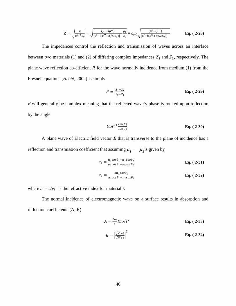
Moreover, the intrinsic electromagnetic impedance of a material may be given generally
by
Page 40
40
=
Eq. ( 2-28)
The impedances control the reflection and transmission of waves across an interface
between two materials (1) and (2) of differing complex impedances and , respectively. The
plane wave reflection co-efficient for the wave normally incidence from medium (1) from the
Fresnel equations [Hecht, 2002] is simply
Eq. ( 2-29)
will generally be complex meaning that the reflected wave`s phase is rotated upon reflection
by the angle
Eq. ( 2-30)
A plane wave of Electric field vector that is transverse to the plane of incidence has a
reflection and transmission coefficient that assuming
is given by
Eq. ( 2-31)
Eq. ( 2-32)
where ni = c/vi is the refractive index for material i.
The normal incidence of electromagnetic wave on a surface results in absorption and
reflection coefficients (A, R)
Eq. ( 2-33)
Eq. ( 2-34)
Page 41
41
2.6 Dielectric Measurement Techniques
Dielectric measurements of various materials are finding increasing application with the
advances in new materials. Dielectric measurements involve the measurement of the complex
relative permittivity of a sample under test for a specific orientation of electric field and
frequency and several methods exist [Chen et al., 2004; Clarke et al., 2003; Egorov, 2007;
Gregory and Clarke, 2006; Kaatze and Feldman, 2006; Krupka, 2006; Stuchly and Stuchly,
1980; vonHippel and Labounskyl, 1995]. The measurement methods can be categorized into two
main groups that are referred to as i) wave methods and ii) impedance methods [Clarke et al.,
2003]. The wave methods further divided into two types depending on whether propagating or
standing waves are employed. These different approaches are briefly reviewed below.
2.6.1 Time domain methods
Time domain reflectometry (TDR) is a popular method to obtain estimates of the water
content in a material by essentially measuring the transit time of EM pulse through the material
being examined. As the theoretical discussions above reveal, the transmission speed depends on
the dielectric properties. The first application of TDR was soil-water measurements [Topp et al.,
1980], where travel times in co-axial probes the annulus of which were filled with the saturated
soils were measured by fitting tangent lines to collected wave form features. The applications of
this method can be found in the literature [Chung and Lin, 2009; Dalton et al., 1984; Dirksen
and Dasberg, 1993; Jones and Friedman, 2000; Malicki et al., 1996; Robinson and Friedman,
2003; Whalley, 1993]. However, this method has some limitations. This method only provides
one value of travel time and hence a single apparent measure of the dielectric permittivity.
Previous studies reported the erroneous permittivity due to the uncertainty in the measurement of
travel time for soil water content using TDR [Hook and Livingston, 1996; Pepin et al., 1995; Sun
Page 42
42
et al., 2000]. Moreover, methods using TDR are not suitable to determine the frequency
dependence of electrical properties of soil or related materials.
2.6.2 Standing wave methods
The dielectric properties of rocks and minerals can be measured in the frequency range of
300 MHz to 2400 MHz using standing wave method [Parkhomenko, 2012]. In this method a
movable detector is shifted within a transmission line along a standing wave pattern. The
permittivity of the sample is calculated by measuring the input impedance of the coaxial section
of a waveguide where the rock samples are inserted, The input impedance is acquired from
voltage to standing wave ratio for both circumstances (empty and filled with the sample) and the
phase shift caused by the sample in the coaxial section [Hoekstra and Delaney, 1974]. This
method requires relatively large sample sizes.
2.6.3 Frequency Domain Methods
In frequency domain reflectometry (FDR) method, the dielectric permittivity is usually
calculated from the coefficients of EM wave pulse reflection and transmission measured using a
network analyzer [Krupka, 2006]. The amplitude and phase of the reflected waves vary with
frequency; and therefore the coefficients are complex numbers that account for the phase and the
amplitude of the travelling wave [Clarke et al., 2003]. Network analyzers are devices that
normally are used to determine the response of electronic devices at RF and microwave
frequencies. These devices are usually called the ‘device under test’ or DUT. This is done so that
their applicability in circuits of such frequencies can be properly assessed. Their basic operation
relies on sending out an EM pulse of known strength and comparing this with the reflection that
comes back along the same transmission line. The reflection co-efficient so determined allows
the impedance of the device to be calculated [Agilent, 2003]. The same equipment can be
Page 43
43
adapted to measure the impedance of materials although this can be problematic if the impedance
of the material differs significantly from that for the instrument itself. The range of frequencies
of applicability of such instruments is also narrow.
2.6.4 Impedance Methods
Permittivity measurements using impedance methods rely on the impedance
measurements. The best known device for impedance measurements is Schering bridge which is
similar to a Wheatstone bridge [vonHippel, 1954]. The unknown impedance can be obtained
from the other bridge elements. However, the bridge method encounters a leakage current at
higher frequency (above 1 MHz). Moreover, for the measurement of permittivity, the sample is
placed between two plates, but if the thickness of the sample is not uniform that results the non-
parallel plates as well as air gaps, might produce erroneous permittivity values. Impedance can
also be calculated by measuring the current and voltage across a low value resistor.
2.6.5 Current-Voltage IV methods
This is perhaps the simplest method and as the ‘IV’ method was traditionally applied at
lower frequency ranges. In our study we use a higher frequency RF-IV method developed by
Agilent [Agilent, 2005] but further details are delayed till later sections. The essential
components of an IV measurement system is shown in Fig. 2-5 in which the material to be tested
lies between the two plates of a parallel plate capacitor. This is only for purposes of illustration
as the RF-IV system used later uses instead and open ended co-axial configuration. The parallel
plate capacitor by itself with no dielectric material within it will have an ideal capacitance simply
given by
where is the area of the plates, is their separation distance, and is the
permittivity of free space described earlier. It is important to note that this ideal capacitance
Page 44
44
depends only on the geometry of the capacitor; the open ended co-axial capacitor used in the
actual measurements will have its own value and this is essentially determined empirically as
part of the calibration procedure in order to account for variability (see also [Skierucha et al.,
2004].
If we were considering the simple case of constant direct current (DC) then inserting a
dielectric material of permittivity r gives a capacitance of . Consequently if one can
leave the charge Q constant across the plates then one can, in principle, measure r’ by simply
seeing how much the voltage across the plates would change once the dielectric is inserted.
Since in this case = , then simply .
The situation is somewhat different should the material be subject to an alternating
current (AC) field which is the situation we must consider here (see for example [Rawlins,
2000]. Let us first examine the case of a perfect (i.e. lossless with = 0). Consider the voltage
source providing a continuous harmonic signal at constant circular frequency = 2f and the
voltage across the capacitor is described as . The charge on the capacitor must,
too, then vary at the same frequency according to and as such a current must also
flow back and forth. The charging, and consequently the current flowing, is at a maximum when
the rate of change of the voltage is greatest; and this occurs when . When reaches
its extremum values then its rate of change vanishes indicating that no charging takes place and
the current goes to 0. In other words ‘lags’ by a quarter of a cycle described in time as
or equivalently as a phase angle = 90° = /2. As a result for this perfect dielectric
.This gives a relationship between current and voltage with the capacitor
essentially opposing the change of voltage; with the analogy to Ohm’s law for the DC case, we
can define the impedance of this capacitor to be Z = Vo/Io which has units of Ohms. Further, on
Page 45
45
average the capacitor opposes the current flow according to a quantity called the capacitive
reactance = 1/ that for this perfect case is the same as the impedance Z.
Suppose now that the dielectric is no longer lossless and as such one must in addition to
the capacitive reactance XC include a resistance R to describe it via ; and the
magnitude of the impedance now becomes |Z| = (R2 + XC
2)1/2
. Harmonic current is still
generated by application of the voltage V(t) but now the phase angle is now less than /2 and is
given by any of
. It is worthwhile noting that the loss
angle mentioned above is related to the phase angle according to
(see [vonHippel,
1954]). The current now becomes I(t) =Ioei( t+)
allowing a complex impedance Z = |Z|ei
=
(Vo/Io)ei
. Therefore the complex impedance can be determined in an IV measurement by simply
determining the maximum values of V(t) and I(t) and by finding the time shift dt between them.
This time shift is then converted to the phase delay angle .
We can now define a complex capacitance C( ) = Co[εr’( ) + iεr’’( )] =[i Z( )]
where again Co is the empty cell capacitance that depends on the experimental geometry. Hence
determining the complex dielectric permittivity r( ) using the IV method depends on the ability
to determine Z( ) (see Section 9.1 of [Czichos, 2006].
Page 46
46
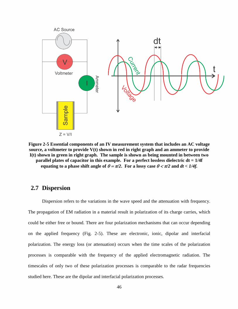
Figure 2-5 Essential components of an IV measurement system that includes an AC voltage
source, a voltmeter to provide V(t) shown in red in right graph and an ammeter to provide
I(t) shown in green in right graph. The sample is shown as being mounted in between two
parallel plates of capacitor in this example. For a perfect lossless dielectric dt = 1/4f
equating to a phase shift angle of /2. For a lossy case /2 and dt < 1/4f.
2.7 Dispersion
Dispersion refers to the variations in the wave speed and the attenuation with frequency.
The propagation of EM radiation in a material result in polarization of its charge carries, which
could be either free or bound. There are four polarization mechanisms that can occur depending
on the applied frequency (Fig. 2-5). These are electronic, ionic, dipolar and interfacial
polarization. The energy loss (or attenuation) occurs when the time scales of the polarization
processes is comparable with the frequency of the applied electromagnetic radiation. The
timescales of only two of these polarization processes is comparable to the radar frequencies
studied here. These are the dipolar and interfacial polarization processes.
Page 47
47
Over the range of radar frequencies, all heterogeneous materials and materials that
contain permanent dipoles (like water) will experience dispersion. Rocks are mostly made of
heterogeneous materials and may contain free water which is perhaps the best known dipolar
molecule. Therefore they are expected to show dispersion behavior if water is present. In the
absence of water the dispersion is usually minute. The addition of a small amount of saline water
however results in strong dispersion especially at the lower frequencies of the GPR (up to 500
MHz).
Figure 2-6 Different polarization processes occur at different frequencies causing dielectric
dispersion (Ref after (Agilent)).
2.7.1 Orientation or Dipolar polarization
Molecules are formed from the combination of various atomic elements each of which
will have its own distinctive structure of the cloud of electrons surrounding it. Pure elements,
too, can form into crystals that are anisotropic structures and result in the disruption of the
electron clouds. An imbalance in the charge distributions will be created due to this
rearrangement of electrons with unequal balance between negative and positive charge.
Moreover, this imbalance in charge distribution will create a permanent dipole moment. The best
Page 48
48
example of such a ‘polar’ molecule is water whose structure that contains two H atoms at the
equilibrium angle of 104.5°. Hence, once water is placed in an electrical field, this imbalance
places a substantial torque on the molecule forcing it to line up with the electrical field direction.
In absence of an electric field all of the moments of the liquid polar water would be
randomly oriented and these random orientations cause the material to be non-polarized. From
Fig. 2-7, we can see that the presence of an electric creates a torque on the dipole and the
dipole will align along the applied electric field causing dipolar or orientation polarization. The
torque will change with the changes in the electric field direction.
Figure 2-7 Dipolar rotation in the electric field (Ref after (Agilent)).
As noted earlier, a propagating EM wave is described in part by a harmonically varying
field with time. This causes the water molecule to be physically oscillated back and forth with
the field variation. However, the molecules cannot do this freely as they collide with one another
in the fluid and this causes a ‘friction’ between them that contributes to the loss of energy which
heats the material. In relaxation frequency range which occurs mostly in the microwave
frequency region, the dipole orientation will create a variation in both and . Liquids and
gases mainly show this type of polarization.
Page 49
49
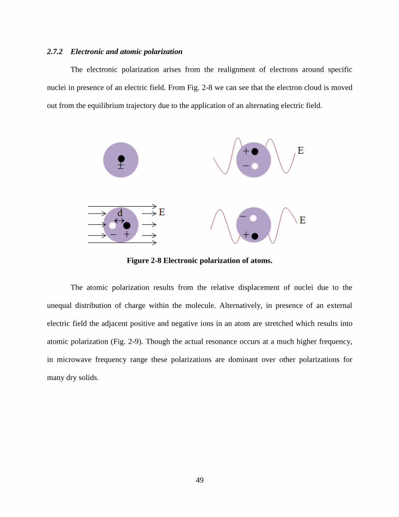
2.7.2 Electronic and atomic polarization
The electronic polarization arises from the realignment of electrons around specific
nuclei in presence of an electric field. From Fig. 2-8 we can see that the electron cloud is moved
out from the equilibrium trajectory due to the application of an alternating electric field.
Figure 2-8 Electronic polarization of atoms.
The atomic polarization results from the relative displacement of nuclei due to the
unequal distribution of charge within the molecule. Alternatively, in presence of an external
electric field the adjacent positive and negative ions in an atom are stretched which results into
atomic polarization (Fig. 2-9). Though the actual resonance occurs at a much higher frequency,
in microwave frequency range these polarizations are dominant over other polarizations for
many dry solids.
Page 50
50
Figure 2-9 Atomic polarization between ions
It is important to take the inertia of orbiting electrons into consideration at infrared and
visible light range. From Fig. 2-6 we can find that the damping effect of a mechanical spring-
mass system and that of atoms containing orbiting electrons are similar except that the resonance
frequency the amplitude associated with the oscillation will be smaller. The electronic and
atomic polarizations are almost lossless far below resonance frequency and contribute a little
to . The resonant frequency is denoted by a resonant response in and a peak of maximum
absorption in . Above the resonance these mechanisms have no contribution.
2.7.3 Ionic Polarization
Ionic polarizations are mostly seen in solids having internal dipoles. These dipoles cancel
each other out and unable to move under the application of an external electric field. The electric
fields slightly displace the ions to induce the net dipoles.
2.7.4 Response of Different Polarization to Applied Field Frequency
The above mentioned polarization mechanisms are functions of the applied field
frequency. When the applied field frequency is quite low, all the mechanisms can easily reach to
their steady peak value. With increasing frequency it becomes difficult for the polarization
Page 51
51
system to reach to the desired peak value. From Fig. 2-6 we can see that when the applied field
frequency is to Hz, the dipolar (orientation) polarization becomes unable to reach to
its equilibrium value and starts contributing less to the total polarization as frequency increases
further. At high electric field frequencies (like infrared and visible light range), electronic and
atomic polarization can occur. Each dielectric mechanism has a characteristic cut-off frequency.
As the cut-off frequency increases, the slower mechanisms cannot be stimulated and only the
faster mechanisms can contribute to . The dielectric loss will be peaks at each critical
frequency.
2.7.5 Interfacial or space charge polarization
The above mentioned polarization mechanisms occur only when charges are locally
bound in atoms or molecules. But there is another polarization mechanism where the charge
carriers can migrate through the material in presence of an electric field. When the motion of
these migrating charges is inhibited it causes a polarization mechanism which is called interfacial
or space charge polarization. The motion due to migration can be hindered when charges cannot
freely discharge at the electrodes. The interfacial polarization occur when there is a build-up of
charges (which can be either free or bound) at the interface. The field distortion caused by the
accrual of these charges increases the overall capacitance. Therefore, it will create an increase in
as the effective capacitance of the system increases.
The response of a charge to the nearby charge particles depends on the thickness of the
charge layers compared to the particle dimensions. For thin and very small charge layers it will
independently respond to the nearby charge particles. The behavior of this type of polarization
depends on the frequency range. At low frequencies the charges have sufficient time to gather at
the borders of the conducting regions which causes an increase in . On the contrary, the charges
Page 52
52
do not have enough time to gather at higher frequencies. So the polarization is minimal as the
charge displacement is small compared to the dimensions of the conducting territory. These
frequency effects are known as the Maxwell-Wagner effects.
It is possible to take place some other dielectric mechanisms in this low frequency
territory. For example, when the charge layer thickness is the same or larger than the particle
dimensions a colloidal suspension exists. Note that colloidal suspension refers to a mixture of
particles where colloids (dispersed insoluble particles having the size in the range of 1 to 1000
nanometers) are suspended in a continuous phase of other particles. The response is now
dependent on the charge distribution of adjacent particles. Consequently, Maxwell-Wagner effect
is no longer applicable [Dyer, 2004].
2.8 Dielectric Relaxation
When the applied electric field is removed one might expect the polarization field will
also fall zero instantaneously. In real cases, however, it takes some time for the dipoles to return
to their random state. The time required for the dipoles to revert to their primary random state is
known as relaxation time expressed by . In other words, relaxation time measures the mobility
of molecules in a material.
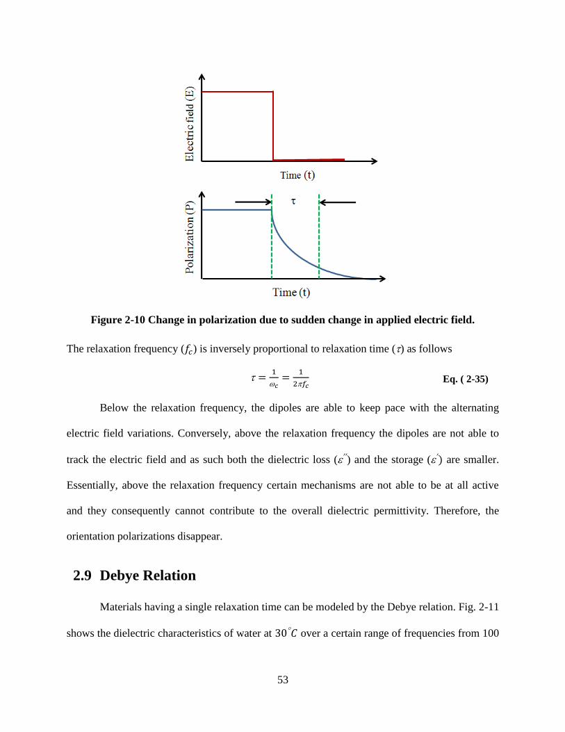
Fig. 2-10 shows the relaxation time of a dielectric material due to sudden drop in the
electric field. All the above mentioned polarization mechanisms can operate until a certain
frequency range. After that frequency all the mechanisms will disappear due to any increase in
frequency. This frequency is known as relaxation frequency which is represented by .
Page 53
53
Figure 2-10 Change in polarization due to sudden change in applied electric field.
The relaxation frequency ( ) is inversely proportional to relaxation time ( ) as follows
Eq. ( 2-35)
Below the relaxation frequency, the dipoles are able to keep pace with the alternating
electric field variations. Conversely, above the relaxation frequency the dipoles are not able to
track the electric field and as such both the dielectric loss ( ) and the storage ( are smaller.
Essentially, above the relaxation frequency certain mechanisms are not able to be at all active
and they consequently cannot contribute to the overall dielectric permittivity. Therefore, the
orientation polarizations disappear.
2.9 Debye Relation
Materials having a single relaxation time can be modeled by the Debye relation. Fig. 2-11
shows the dielectric characteristics of water at over a certain range of frequencies from 100
Page 54
54
MHz to 1 THz. From Fig. 2-11 we can see that dielectric storage ( ) is constant above and
below relaxation frequency whereas dielectric loss ( ) is small above and below the relaxation
frequency.
Figure 2-11 Debye relaxation for water at 30 °C (ref after (Agilent)).
The Debye theory of complex permittivity gives the permittivity in terms of
Eq. ( 2-36)
and
Eq. ( 2-37)
where, ( is the frequency). For , and ,
From the Debye relation, it is possible to find out the dependence of permittivity on the
applied frequency. It can be seen that decreases with increasing frequency while will have a
maximum value. decreases due to the phase lag between the dipole alignment and the electric
field.
Page 55
55
2.10 Cole-Cole Diagram
The Debye relation works if only one pure type of relaxation mechanism exists, but this
is rarely the case and a number of different effects can all be active. Instead, the complex
permittivity is often displayed using what is called a Cole-Cole diagram. It is one of the better
approximations in most of the dielectric cases though Debye relation is also very important. The
Cole-Cole diagram is simply a plot of on the Y-axis and on the X-axis. Cole-Cole diagram
can be expressed by the following equation
Eq. ( 2-38)
where is the complex dielectric permittivity, is the angle between the real axis and the high
frequency intercept line drawn to the center of the semi circle.
Figure 2-12 Cole-Cole representation of the Debye model of water at 300C. (ref. after
(Agilent)).
Fig. 2-12 shows the maximum value of for a dielectric material with a single relaxation
frequency. The frequency moves counter clockwise on the curve. If a material has multiple
relaxation frequencies which are symmetrically distributed will be a semi-circle. On the other
Page 56
56
hand, in case of non-symmetrical distribution it will be an arc. In both cases the center will be
lying below the horizontal axis.
2.11 Debye and Cole-Cole diagrams for water from experiments
Fig. 2-13 shows the Debye plot for water from our experimental data. In this plot real and
imaginary permittivities are plotted against frequency. The real permittivity started decreasing at
~0.5 GHz. On the other hand the imaginary permittivity started increasing sharply around that of
0.5 GHz. We can compare our measurement result with the Debye approximation in Fig. 2-11. It
was not possible for us to figure out the relaxation frequency as our measurement frequency was
not high enough like the frequency range used in Fig. 2-11. Fig. 2-14 represents the Cole-Cole
plot (left) and a circle fit (right) for water. From the circle fit we can find that the center was not
exactly at zero. But an ideal Cole-Cole representation starts from zero. Therefore we can
conclude that out experimental data for water was not a perfect Cole-Cole representation.
Page 57
57
Figure 2-13 Debye plots for water from the experimental data
Page 58
58
Figure 2-14 Cole-Cole plot for water from the experimental data (left). Circle fit of the data is also shown (right).
Page 59
59
2.12 Mixing Theories
The theory of the power dissipation of the electromagnetic wave in a medium is straight
forward for a single component, homogeneous, isotropic system. However, naturally occurring
rocks and minerals are not purely homogeneous systems, but are a mixture of minerals and fluids
within the pore spaces. Most rocks are also porous and to some extent saturated with liquids. In
addition, rocks are composed of grains with different sizes, shapes, and distributions. The
frequency dependent space-charge interactions at the fluid-mineral interfaces, too, influence the
observed dielectric properties particularly at low frequencies. All of the mentioned properties of
the rock have a measurable effect on the complex dielectric permittivity and therefore complicate
the interpretation of the GPR and TDR data. The effect is prominent on the dielectric permittivity
measurements of many minerals particularly those for which appropriate single crystals are not
available. For this reason, dielectric permittivity of these materials have been measured using
mineral powders mixed with air or other well characterized fluids [Arai and Binner, 1995; Avelin
and Sihvola, 2002; Brovelli and Cassiani, 2008; Davies et al., 2005; D. C. Dube, 1970; D. C.
Dube and Parshad, 1970; D. C.; Dube et al., 1971; Economos, 1958; Hilhorst et al., 2000;
Kingery et al., 1976; Martinez and Byrnes, 2001; Matzler, 1998; Mdarhrj et al., 2008; S Nelson
et al., 1989; S. O. Nelson, 1983; 1994; 2001; 2005; S. O.; Nelson and Bartley, 1998; Olhoeft,
1981; Payne, 1973; Reynolds and Hough, 1957; Robinson and Friedman, 2005; Robinson et al.,
2003; Rust et al., 1999; Spanoudaki and Pelster, 2001; Widjajakusuma and Biswal, 2003].
Mixing technique has an advantage over single crystals, assuming the sample's mineral grains
are randomly oriented; the dielectric permittivity may be treated as a scalar. However, a major
disadvantage of this method is that many such samples are porous and heterogeneous by their
nature. Consequently, it is often necessary to measure the permittivity at known density (or
Page 60
60
equivalently porosity) and then on the basis of a numerical or theoretical model to extrapolate
this value back to vanishing porosity [S Nelson et al., 1989; Robinson and Friedman, 2003].
Note porosity is sometimes considered as an additional control to the dielectric properties of
advanced components in the electronics industry [Kata and Shimada, 1992].
Mixing models attempt to predict permittivity of different mixtures depending on the
selected input parameters. Several mixing models have been proposed in the literature to predict
dielectric properties of rocks and minerals. These models have been classified into four broad
categories: effective medium, empirical or semi-empirical, phenomenological and volumetric
[Knoll, 1996; Martinez and Byrnes, 2001]. Every model has some advantages and disadvantages
depending on the assumptions.
In the effective medium approach the dielectric permittivity estimation is based on
successive substitutions [Sen et al., 1981]. The Bruggeman-Hanai-Sen (BHS) equation is an
example of effective medium theory. This model is robust for the materials with known
geometries such as water-saturated materials with non-interacting components. However, the
model is not easy to implement and is rarely used in practice.
The empirical or semi-empirical models are based on the mathematical equations
(logarithmic or polynomial) that relate dielectric and other measurable properties. These models
are easy to implement for complex materials. However, these methods are not suitable for data
sets that include the materials with different mineralogies, porosities as well as water saturations
[Dobson et al., 1985; Olhoeft and Strangway, 1975; Topp et al., 1980; Wang and Schmugge,
1980]. Logarithmic and polynomial type theories represent empirical and semi-empirical models.
The phenomenological model is based on the relationship between frequency dependent
behavior and characteristic relaxation times. It is not necessary to know the component
Page 61
61
properties or geometrical relationship in this model but the model depends on frequency specific
parameter. Cole-Cole and Debye models are usually used in the phenomenological approach
[Powers, 1997; Wang and Schmugge, 1980].
Another important approach for mixing models is volumetric model in which dielectric
properties are estimated from the relationship between the bulk dielectric constant of multiphase
mixtures with that of its constituents. Examples of this include the Complex Refractive Index
(CRIM) and the Lichetenecker-Rother formula. However, the micro-geometry and the
electrochemical interactions between the components are not considered in these types of models
[Knoll, 1996; Lichtenecker and Rother, 1931; Roth et al., 1992; Wharton et al., 1980].
In addition, Cosenza et al. classified these into three groups: statistical, numerical and
effective medium theory [Cosenza et al., 2003]. In the statistical approach the permittivity is
calculated by assuming that the porous medium is a 3-D network of capacitors. In the numerical
approach the permittivity estimation is based on the numerical solution of Maxwell’s equations
at the microstructure level. Both the statistical and numerical techniques require detailed
knowledge of the material’s microstructure.
The determination of the effective dielectric properties of a mixture has been studied for
more than 100 years and consequently a large number of effective medium theories have been
proposed [Koledintseva et al., 2009; Sivhola, 2002; van Beck, 1967]. In the effective medium
theories the "effective" bulk permittivity is calculated from the individual permittivity of the
medium constituents variously weighted by the volume average factor. The basic idea of
effective medium theory is to focus on a particular inclusion and it assumes that the inclusion is
surrounded by an effective homogeneous medium [Choy, 1999; Myroshnychenko and Brosseau,
Page 62
62
2005]. This turns out that there is no correlation between the inclusions in effective medium
theories.
Following the lead of many authors we will here attempt to evaluate the effectiveness of
a number of different mixing models that are employed in the literature. There are numerous
reviews on this topic from various perspectives that may be found (e. g., [A. H. Sihvola, 1989] ).
For each we will provide a brief rationale as to how the method was developed and what its
major underlying assumptions and limitations might be. It is important to note that most of the
mixing models and bounds described here do not contain any detailed information on the
material structure and rely solely on knowledge of the constituents permittivities and volume
fractions in the mixture.
One of the most popular and widely used formulations for calculating effective
permittivity of dilute mixtures is the Maxwell-Garnet (MG) theory which was first formulated
for spherical inclusions [Bergman and Stroud, 1992; Sihvola, 1999]. Let us consider a two-phase
mixture which consist of two dielectric components; one of them is background that works as a
host material, and the other one is inclusion that is embedded as a guest material. The dielectric
permittivity and fractional volume of the background material are denoted as and
respectively while and are the permittivity and fractional volume of the inclusion materials.
The Maxwell-Garnet [1904] mixing rule (also called the Clasisus-Mossotti approximation or the
average T-matrix approximation [Sen et al, 1980] is perhaps the most widely applied in part
because of its simplicity for the two-phase mixture can be written as
Eq. ( 2-39)
where is the effective dielectric permittivity of the mixture. Maxwell-Garnett developed this
theory by essentially summing the individual polarizability of individual inclusions generally of
Page 63
63
spherical (or ellipsoidal) shape in order to exactly calculate the induced field within the
background host material which is then approximately modified to account for the interactions
between the inclusions. This is sometimes referred to as a ‘raisin pudding’ model. Sihvola [1999]
gives a basic yet detailed discussion that goes through the derivation. The Maxwell-Garnet
model works well for small concentrations of inclusions in a dielectric host (inclusion volume
fraction <0.1) [Spanoudaki and Pelster, 2001]. The Maxwell-Garnett theory can also be applied
to inclusions of any arbitrary ellipsoidal shapes such as spheroids, cylinders and disk through the
introduction of depolarization factors. However, any other shapes that are not perfectly
ellipsoidal can only be modeled by any closest ellipsoidal shapes, which may provide erroneous
results [Avelin and Sihvola, 2002]. Robinson and Friedman suggested that the Maxwell-Garnet
theory ‘adequately’ described the permittivity of mixtures of glass beads and various fluids
particularly for fluids with a large permittivity. The Maxwell-Garnett model, too, can be
extended easily to predict the effective dielectric properties of a material with more than two
constituents [Sihvola, 2013]
It is important to note that one must take great care in deciding which material is inclusion and
which is background. It is easily demonstrated by examination of Eq. 2-39 that they are not
invertible and the predicted values for the same compositions can be quite different depending
upon which role the materials play. This should not be surprising as the Maxwell-Garnett
formulation does contain to a degree some information on the structure of the material and how
the fields within it are produced. That said, this issue does further suggest that the Maxwell-
Garnett model is valid for dilute inclusions.
Page 64
64
Bruggeman [1935] proposed a formula which goes by various names such as the
symmetric mixing rule or the coherent potential approximation [Sen et al, 1980] which is given
below
=0 Eq. ( 2-40)
The main premise of this rule is that there is no one constituent that is considered as either an
inclusion or as the background material, the contributions of both are considered equally. As
noted by [Sihvola, 2013] one could interpret this model as having the background consist of the
homogenized medium itself against which the polarizations may be found. This means there is a
fundamental distinction between the Bruggeman and the Maxwell-Garnett models. For denser
mixtures or composites Bruggeman theory works better than the Maxwell-Garnett theory.
Power law models are often used to calculate the effective dielectric permittivity, these
are essentially weighted averages. For a two-phase mixture, the formula is
Eq. ( 2-41)
where c is a fitting factor (1 ≥ c ≥ -1) [Brovelli and Cassiani, 2008; Guéguen and Palciauskas,
1994] have referred to this as the ‘Litchteneker-Rother’ equation. Various authors have used
differing values of c for a variety of reasons and some examples of power law theories are
complex refractive index method (CRIM); Landau, Lifshitz, Looyenga (LLL) equation; and
Lichtenecker logarithmic mixture equation. These models are briefly discussed below.
The CRIM formula assumes c = ½ and this essentially is equivalent to assuming that the
refractive index of the mixture is the arithmetic mean of the constituents refractive indices
weighted by their volume fractions. This is also called the Birchak formula [Sihvola, 2013]. This
follows from the fact that the refractive index n = c/v = c( )1/2. For a two-phase mixture, the
CRIM equation [Brovelli and Cassiani, 2008] is
Page 65
65
Eq. ( 2-42)
Probably because of its simplicity, it has been widely applied in Geophysical studies particularly
with regards to ground penetrating radar where wave speeds are measured.
Looyenga [1965] developed a model in which , which is now often referred to as the
Landau-Lifschitz-Looyena (LLL) formula and claimed on the basis of comparison to earlier
measurements of the dielectric permittivity of a mixture of glass beads and carbon tetrachloride
that it was superior to either the Maxelll-Garnett or the Bruggeman models. Looyenga developed
his model from first principles by calculating the average dielectric permittivity should a small
sphere of permittivity 2 be moved about within a larger sphere of permittivity 1. The LLL
formula then can be written as
Eq. ( 2-43)
Lichtenecker and coworker [Lichtenecker and Rother, 1931] developed essentially an
empirical expression that would provide an intermediate between the Weiner bounds. Essentially
his model is the geometric mean value which can be written
Eq. ( 2-44)
This empirically derived logarithmic mixing model is also used for fitting experimental
data; however previous work [Payne, 1973] revealed that the logarithmic fitting model might
work by coincidence. [Reynolds and Hough, 1957] provided a particularly critical review of this
model. More recently Zakri et al. [1998] claim that there is some situations where it is
theoretically justified if the shapes of the inclusions take a beta function distribution.
Sen and coworker [Sen et al., 1981] derived what they refer to as a ‘self-consistent’
formula for a two-phase mixture which is given below
=1- Eq. ( 2-45)
Page 66
66
where p is a constant which depends on the geometrical shape of the rock grain. If the rock grain
is spherical, then p =1/3. Thus the Eq. (2-45) becomes
=1- Eq. ( 2-46)
The derivation of this equation essentially relies on the fact that the pore space network
in earth materials remains connected even at very low porosities. As such, they assume that the
material can be modelled as mineral grains coated with water and they go forward by assembling
the medium from coated grains of arbitrary size. It is important to note that in the same paper
Bruggeman [1935] followed by Hanai [1968] developed similar expressions to Eq. 2-46 that start
with the Maxwell-Garnett Eq. 2-39.
From different mixing theories we can obtain different effective permittivity values.
However, these predictions are limited by some bounds. The mostly used bounds are Wiener and
Hashin-Shtrikman. The Wiener bounds are as follows
Weiner upper bound (Wiener+)
Eq. ( 2-47)
Weiner lower bound (Wiener-)
Eq. ( 2-48)
These Wiener bounds correspond to capacitors which are arranged in either parallel or series in a
circuit and providing the upper or maximum and lower or minimum bounds [Neelakanta, 1995].
Note Eq. (2-47) is the maximum for both the and as well as Eq. (2-48 is)
minimum for both cases. It is also useful to make the comparison of the upper (Eq. 2-47) and
lower (Eq. 2-48) to the limiting values of c = 1 and c = -1 in the Litchteneker-Rother Eq. 2-41
above.
Page 67
67
Hashin-Shtrikman used a variational approach where the upper and lower bounds are shown by
the following equations. The Hashin-Shtrikman upper bound (HS+)
Eq. ( 2-49)
The Hashin-Shtrikman upper bound (HS-)
Eq. ( 2-50)
We have used all the above mentioned mixing theories to create theoretical models later
on in chapter 4. Our rational for using these different models, all of which are popular within the
literature whether justified or not, is to see which might best describe our materials such that it
could be used in a practical way for predicting dielectric GPR permittivities and wave speeds.
2.13 Conclusions
To have an idea about the dielectric measurements we have discussed all the relevant
theoretical background of dielectric permittivity and this section also included a review of the
pertinent literature. At first we have discussed about dielectric materials, electromagnetic wave
propagation and then we have presented different dielectric measurement techniques. At the end
of this chapter different mixing theories were presented. We have also presented a literature
review regarding to these theories.
Page 68
68
CHAPTER 3. METHODOLOGY
In this chapter we present a detailed discussion of the measurement protocols, the sample
preparation techniques, and the advantages and limitations of both measurement system and
sample preparation technique.
3.1 Measurement System
The measurement system is comprised of an impedance or material analyzer, an open
ended coaxial probe, and the associated software necessary to operate the instrument. The
impedance analyzer is an Agilent E4991A RF impedance or material analyzer in addition with a
coaxial probe and software which are included in Agilent 85070E dielectric probe kit shown in
Fig. 3-1. Moreover, a computer is connected to the equipment to store the measured dielectric
data. The coaxial probe in Fig. 3-2 has a 3.5 mm connector which is supported by a 19 mm
diameter flange. A cross section of the sensor is shown in Fig. 3-2 (on the right). The flange
allows us to perform measurements on smooth and flat surfaced solid samples as well as
immersed within liquids and semi-solids. This probe can withstand a wide temperature range
from -40 to +200ᵒ C. This instrument is designed primarily for measuring the complex dielectric
constant from the direct measurement of both current and voltage associated with a given
harmonic input of nonmagnetic, isotropic and homogeneous materials over the frequencies
ranging from 10 MHz to 3 GHz.
The calibration of the probe is done using three standards that are usually an open circuit,
a short circuit, and pure (deionized) water. The dielectric permittivity of water is 80 [Ellison et
al., 1996]. Water is often used as a standard because of its well-known dielectric properties. This
Page 69
69
instrument provides a measure of the real part of the dielectric permittivity with an uncertainty of
about 1% although these uncertainties are higher for the complex components leading to a 5%
uncertainty in the quality factor Q [Agilent, 2005].
Figure 3-1 Measurement system: Agilent 4991A RF Impedance/Material Analyzer (left),
coaxial line sensor (middle), and a magnified picture of the 19 mm diameter sensor (right).
Measurements may be obtained over a frequency range of 10 MHz to 3 GHz
From Fig. 3-2 (right) we can see that the diameter of the outer face of the probe is
and for accurate measurement there should no air gaps between the face of the probe and the
material surface. Therefore in this experimental setup, the sample is required to be more than
in diameter with an ‘adequately’ flat surface so that there is no air gap between the
sample and the face of the sensor. The manufacturer recommends that the thickness of the
sample should be greater than to avoid edge effects. The calibration can be done
from room temperature up to 40⁰ C without significant error due to temperature change [Gregory
and Clarke, 2007].
This instrument allows us measurement of the dielectric permittivity under a variety of
different sample geometries. However, this open-ended coaxial probe method is practical for the
study of earth materials that are difficult to machine into 3 mm thick wafers.
Page 70
70
Figure 3-2 Coaxial probe (left) and a cross section of the sensor. The electric field lines
fringe from the end of the sensor into the sample under measurement.
3.2 RF I-V Technique
The basics of the current-voltage measurement technique were provided in Section 2.6.5
and to briefly review this necessitated the determination of the complex impedance Z( )
applying a V(t) and measuring the resulting I(t). which could then be directly related to the real
and imaginary parts of the complex dielectric permittivity r( ). RF I-V method was used as our
measurement technique as it provides better impedance measurement capabilities than other
existing techniques [Agilent, 2001]. The instrumental setup consists of an impedance matched
measurement circuit (50 Ω) and a precision co-axial test port for operation at higher frequencies.
It is composed of two types of basic circuit configurations as shown in Fig. 3-3. Two different
types of voltmeter and current meter arrangement provide low impedance and high impedance
measurements respectively. The impedance of device under test (DUT) is derived from measured
voltage and current values. The current is calculated from the voltage measurement across a
known value resistor (R) [Agilent, 2001].
Page 71
71
In order to measure a low voltage across the low impedance DUT a low impedance type
configuration is used which has a voltmeter adjacent to the DUT for more accurate measurement.
While a high impedance type configuration is required to measure a low test current through the
high impedance DUT and a current meter is used near the DUT to get more accuracy.
The graph, in Fig. 3-3, shows the relationship of the measured vector voltage ratio to impedance.
The solid curves (Rx) in the graph apply to resistive DUTs while the broken curves (Xx) apply to
reactive DUTs. The voltage ratios differ for the reactance and resistance of DUT because the
magnitudes of the vector ratios vary depending on the phase angle relationship between the
DUT’s impedance and the measurement circuit impedance, Z0. The resistive DUTs yield greater
voltage ratios than the reactive DUTs.
Figure 3-3 Basic principle of RF I-V technique and vector voltage ratio relationship (ref.
after Agilent).
The detected voltage ratio is proportional to the impedance implies the gradient of vector
voltage ratio curve is constant over of the range of impedance. Consequently we obtain constant
measurement sensitivity. As the gradient of vector voltage ratio levels off in the high impedance
Page 72
72
or low impedance regions the measurement sensitivity deteriorates. However it is possible to
selectively install the two types of test heads to complement the two measurements ranges.
The vector voltage relationships can be written as
, for low z-type Eq. ( 3-1)
where 100 = Zr represents the roll-off impedance.
And
for high Z-type Eq. ( 3-2)
where Zr = 25.
The RF I-V circuit can be designed for the roll-off impedance (Zr) value that is properly
shifted t wider measurement sensitivity. The Agilent E4991A uses the single test head designed
in such a way so that it can cover a wide impedance range without any need of exchanging the
test heads. Fig. 3-4 represents the vector voltage ratio characteristics of the E4991A.
Figure 3-4 Vector voltage ratio relationship to impedance for E4991A.
Page 73
73
Though it seems the single test head configuration of the E4991A sacrifices a little the
measurable impedance range when compared to the combined impedance range of the low
impedance and high impedance type test heads but in practice, the E4991A’s test head does not
provide such disadvantages, because the specified measurement range in high frequency region
(above 10 MHz) is dominated by the calibration uncertainty [Agilent, 2005]. The advanced
design of the E4991A’s test head ensures high SNR (signal-to-noise ratio) performance superior
to the low and high impedance types of test heads.
3.2.1 Calibration
Outside of factors related to the geometry itself, the accuracy of a measurement system
depends mainly on the accuracy of calibration. The calibration of the open ended coaxial probe
was performed prior to each set of tests using three standards which are: 1) an open circuit 2) a
short circuit, and 3) a reference liquid (de-ionized water). De-ionized water is usually selected
because it is readily available, non-toxic and has well known dielectric properties. The
instrument includes within its operation known measured values of the complex dielectric
constant of water against with the measurement may be compared to provide the calibration.
Further in this study, in order to check the accuracy of the calibration two large high-
purity single crystal evaporites (purchased from Del Mar Photonics) were measured just after the
calibration. These single crystals are halite (NaCl) and sylvite (KCl). At first we placed these
single crystals on the sensor and then took measurements. We repeated the measurement for five
times for each of the crystals and then calculated the average of five measurements. They were
chosen because of their well characterized dielectric properties [vonHippel, 1954; vonHippel and
Labounskyl, 1995; Young and Frederikse, 1973]. These crystals are optically isotropic and
Page 74
74
therefore their dielectric permittivities do not depend on crystal orientation. To get accurate
dielectric data from these types of crystals it is very important to keep them in a humidity free
environment. If we keep it in open places it might absorb moisture and the dielectric data might
not be consistent. This turned out to be a problem later in our study as the cover to the desiccator
that they normally were stored in was left open to the humid atmosphere. Both the and
crystal adsorbed water with the loss of their optical clarity and their measured dielectric
values making them of no use for checking the calibration. In future, workers must take care to
ensure that such crystals are not damaged by exposure to even the small amounts of water in the
relatively dry air within our building.
Measures of the real permittivity from 10 MHz to 3 GHz on these large single crystals
prior to them being damaged are shown in Fig. 3-5. The dielectric permittivity of halite crystal
was measured by Von Hippel [1954] who confirm that there exist only a single value of the
dielectric permittivity at frequencies between 100 Hz and 25 GHz and with his value being equal
5.90. Lowndes also obtained the same value of the real permittivity (which is 5.9 ± 0.02) at
frequencies between 100 Hz and 1 MHz [Lowndes, 1966]. We obtained the real part of the
permittivity of halite and sylvite single crystals were 5.9 and 4.8, respectively (Fig. 3-5).
Repeated measurements at different points on these crystal faces at different times show less than
1% deviation in the measured real permittivity which indicates the consistency of the calibration.
Page 75
75
Figure 3-5 Dielectric permittivity of halite and sylvite single crystal to check the accuracy of calibration of the equipment.
Page 76
76
The imaginary permittivity (Fig. 3-5), on the other hand, was too small to be reliably
measured on any of the pure evaporite samples; they fell below the minimum recommended
value of our measurements system which was 0.05. According to Von Hippel [vonHippel, 1954],
the imaginary permittivity of NaCl crystal is less than 0.003 (at frequency between 100 Hz and
25 GHz). The results, shown in this Fig. 3-5, confirm that the imaginary permittivity is very low
but beyond the resolution of the measurement system.
3.2.2 Advantages and Limitations of the RF IV Method
The coaxial line sensor technique has both advantage and limitations. One of the main
advantage of this technique is that it needs a single flat surface of the sample rather than having
to machine the sample to fit into a measurement cell [Clarke et al., 2003]. Relatively small
samples (of at least 20 mm wide and about 10 mm thick) are required. On the other hand, any air
gap between the sensor and the sample is a main source of error in this technique. This can be a
problem with real earth materials as they are difficult to machine and polish effectively. Further,
even when polished the natural porosity and cracks within such materials will disrupt the proper
flow of current in the material. This issue has led us to develop the cold compression technique
described below. Moreover, during measurement the cable should be stable otherwise it will
create error in the measured dielectric permittivity as well.
3.3 Cold Compression Technique
The problems of attempting to measure the dielectric permittivity of natural samples that
contain micro-crack porosity will become increasingly apparent in Chapter 5. Unacceptable
results on rock core material led us to use samples reconstituted from powdered materials. In
Page 77
77
this section we describe a cold compression technique devised in the laboratory to form such
samples for use. A cold compression technique was used to prepare solid samples from mineral
powder for several reasons:
1) It is not possible to obtain acceptable quality or size single crystals for all minerals.
2) Single crystals have crystallographic orientation effects that might give a wide range of
dielectric permittivity for each mineral due to their anisotropy.
3) The dielectric measurement technique used in our experiment is not suitable for powder.
Moreover, it is very sensitive to heterogeneities in the natural sample and to pores and
cracks on the surface. In order to provide a homogeneous sample with a flat surface free
of cracks cold compression method was designed.
The technique essentially consists of squeezing powder samples at high pressures (up to
300 MPa) for extended periods of time. In this technique, the mineral powder was first ground in
a mortar-pestle. The size of the powder particles are less than . This powder was then dried
in an oven for 2 hours at around to remove all the moisture from the powder. After drying
this powder was then poured into flexible plastic tubing the ends of which were then sealed with
aluminum cylinders. The ends of these cylinders were polished flat. Hose clamps were tightened
around the cylinders in order to hermetically seal the sample. The packing and sealing was
carried out as quickly as possible in order to reduce the opportunity for adsorption of water to the
surfaces of the powders. The sealed tube was then left heated at about for 2 to 3 hours.
This heating was found to improve particle adhesion, and on the basis of experience without this
step single unbroken pieces could not be manufactured. In the final preparation step all of the air
was removed from the sealed powder by an attached vacuum pump and the sample was
vacuumed for at least 1 hour. This pumping helped us removing all the air and this step appears
Page 78
78
to have helped to make samples that held together upon decompression. It is likely that any air
that remained in the pores prior to pressurization of the sample may force its way out of the
sample upon depressurization causing damage.
The assembly was then mounted into a pressure vessel in the Rock Physics laboratory.
The sample was then slowly pressurized to the desired peak pressure (~ 150 MPa to 300 MPa)
depending on the plasticity of the mineral and then left at this pressure overnight (for at least 14
to 16 hours and sometimes longer). The sample then was depressurized slowly. We
depressurized in increments of 10 MPa every 5 minutes, an entire depressurization would usually
take more than 2 hours. Experience showed that those samples rapidly depressurized were weak
and usually failed upon removal from the assembly.
The samples obtained were one inch in diameter and a few centimeters thick, this
depended on the amount of power placed in the assembly. Examples of the synthetic samples are
shown in Fig. 3-6. Because the powder of different minerals possess different elastic and creep
properties, the same value and duration of pressure produces varying porosity for different
mineral powder. For example, pure KCl and NaCl samples were easily fabricated with nearly no
detectable porosity due to their inherent plasticity by applying pressures less than 270 MPa.
Calcium carbonate is much more rigid; porosities of 35% could be achieved by elevating the
pressure to 270 MPa.
Page 79
79
3.3.1 Advantages and Limitations of the Cold Compression Technique
A great advantage of this process was that as samples were prepared from mineral
powder compression, the sample grains would be randomly oriented and due to this dielectric
permittivity the sample could be treated as scalar. As a result, the crystal orientation effect can be
avoided. However, a prominent limitation of this technique is that even after applying high
pressure some mineral samples remain very porous. In addition, this technique is time
consuming (typically 18 to 20 hours required to prepare a single sample).
Figure 3-6 Synthetic sample (NaCl and KCl) prepared using cold compressing technique.
3.4 Material Characterization
A number of additional common experimental methods were employed to further
characterize the materials studied. In particular, it is important to have some understanding of
the composition and of the structure of the materials. We briefly provide an overview of these
techniques here in order that the reader better understand the results in later sections.
Page 80
80
3.4.1 Scanning Electron Microscope (SEM)
The Scanning Electron Microscope (SEM) provides visualization of tiny features of an
object. It is similar to conventional optical microscope but light is replaced by electrons (either
secondary or back scattered electrons). A very thin beam of electrons (primary electrons) from
an electron gun are focused on a small area of a sample kept in the SEM scanner; these electrons
interact with atoms in the sample producing various signals (secondary electrons) that can be
detected and amplified using electron detector and an image is produced. SEM can produce
images submicron resolution. The SEM imaging was done using a Zeiss EVOMA 15™ machine
located at the Earth and Atmospheric Science Department at the University of Alberta. SEM
assists to examine the grain structure and micro features qualitatively.
Before scanning the samples we need to prepare them for the measurements. The samples
(both natural potash and cold compressed) were broken into small pieces as our samples were
larger than the instrument could accommodate. The required size for this type of measurement
should be less than 1.5 cm in diameter and 1 cm high. In our case the broken pieces were around
0.7 to 0.8 cm in diameter and the thickness were around 0.4 to 0.5 cm. Before scanning the
samples were coated with electrically conductive carbon which can prevent electron traps which
might make a brighter image. This type of carbon coating is done by thermal evaporation.
However, sometimes if the sample is thick enough a small amount of colloidal graphite is printed
onto one edge of the samples (used as an adhesive) to bridge the samples to the conductive
substrate or the aluminum stubs. The samples are then kept in an oven overnight for thermal
evaporation.
Page 81
81
3.4.2 Helium Pycnometer
The mineral grain volume and hence grain density of the sample can be measured using a
helium pycnometer. In this work, a multi-pycnometer (Quantachrome MVP-D160-E™) under
helium was used. The pycnometer works based on Boyle’s law which states that at a constant
temperature, the volume of a given amount of ideal gas is inversely varied with the pressure of
the gas. That is,
Eq. ( 3-3)
where and are initial and final pressures of the gas and, , are initial and final volumes.
The pycnometer contains two cells: one is as reference while other is for the sample. The idea is
to fill the reference cell with helium and measure the pressure while the volume of the cell
is known. The helium gas is allowed to flow into the other cell where the sample is placed and
the pressure of that cell is measured. The volume can be calculated from the above Eq. (3-
3) Therefore the Equation becomes
Eq. ( 3-4)
or,
Eq. ( 3-5)
where is the volume of the reference cell, is the volume of the cell containing the sample
and is the volume of the solid portion of the sample. That is, gives the total volume of the
reference cell plus the cell containing the sample minus the grain volume of the sample.
Therefore, the porosity can be obtained using the following Eq.
Eq. ( 3-6)
where is the bulk volume which his the sum of solid sample volume and pore space volume.
Using this technique we have calculated the porosities of couple of our samples.
Page 82
82
As our samples were not of regular shape it was not possible for us to calculate their bulk
volume using the length and diameter of the samples. At first we have used plastic wrapper to
wrap up the samples. We wrapped up the samples using a vacuum sealer to make sure that there
is no air after wrapping up the samples. Then we inserted the samples into the sample cell of the
helium pycnometer and repeated the above mentioned working principle. The volume obtained
after the measurements were considered as the bulk volume with plastic wrapper as the helium
gas could not penetrate the plastic wrapper. Next, we calculated the bulk volume of the plastic
wrapper. By subtracting the bulk volume of the sample with wrapper from the bulk volume of
plastic wrapper we have calculated the bulk volume of the sample. Calculating the porosity of
irregular shaped sample was a novel application of this technique.
3.4.3 Mercury Porosimeter
We measured porosity of a limited number of the samples using a mercury injection
porosimeter. This Porosimeter ('Micrometrics' AutoPore IV 9510™) characterizes porosity of
materials by applying different pressure levels to a sample placed in a Hg bath. A mercury
porosimeter measures the pore-throat size distribution and the measurement is based on forcing
mercury into small spaces, pore throats within the sample [Giesche, 2006]. Therefore, mercury
porosimetry technique can be described using Washburn capillary law:
Eq. ( 3-7)
where represents the diameter of pore throat, is the applied pressure, is the surface tension
of mercury, and is the contact angle. Note the Washburn formula is based on the assumption
that the pores are cylindrical. But there are no cylindrical pores for any porous medium; this
equation is usually used to calculate a pore throat size distribution. This measurement is done by
Page 83
83
measuring the volume of injected Hg to the sample with pressure. The equation used in this
measurement is
Eq. (3-8)
Here is the volume of the mercury injected and P represents the applied pressure. From Eq.
(3-8) we can see that the volume changes with the change of pressure when the mercury injected
into the pore space. Fig. 3-7 shows the plot of incremental and cumulative intrusion with
pressure for a porous NaCl sample. We converted pressure to pore size using Washburn's
equation. The porosity is simply ratio of the volume of the Hg injected at the highest pressure to
the bulk volume of the sample as given by the porosimeter at low pressure.
Figure 3-7 Cumulative intrusion versus pressure for a porous NaCl sample (measured
porosity 4%) using Hg porosimeter.
Page 84
84
3.4.4 X-ray Diffraction (XRD)
X-ray diffraction (XRD) is widely used in geosciences to identify minerals within rocks
particularly the fine grained minerals such clays and mixed layers of clays. The basic principle of
XRD is the constructive interference of monochromatic x-rays within lattice planes of the
minerals. X-ray diffractometers are mainly composed of three parts such an X-ray tube, an X-ray
detector and a sample holder. X-ray radiations are generated in a cathode ray tube. These x-rays
are directed toward the sample after filtering to produce monochromatic x-rays and collimating
them to concentrate. These x-rays interact with the sample and produce constructive interference
when the condition for Bragg's law ( where d is the spacing between the sample,
the wavelength, the diffraction angle) is satisfied. The diffracted x-rays are detected and
processed by the x-ray detector, and each mineral will have a characteristic set of diffraction
peaks that may be used to identify it.
3.4.5 X-ray Fluorescence (XRF) Elemental Analysis
For elemental analysis, x-ray fluorescence (XRF) is widely used. This analytical
technique is advantageous as all kind of samples (solid, liquid or powder) can be analyzed. XRF
provides very accurate and precise measurements and the sample preparation is fast and simple.
The basic principle of XRF is based on the source, samples and the detection system. When a
sample is exposed to a source of high intensity x-rays, the atoms of the samples become
temporarily excited by absorbing energy from the x-rays. If the energy of x-rays is sufficient to
dislodge a tightly-bound inner shell electron, the electron cloud become unstable and the missing
inner shell electron is replaced by an outer shell electron dropping down. Consequently energy is
released in the form of secondary x-rays with energy lower than primary incident x-rays. These
‘fluorescent’ secondary x-rays are highly tuned to the quantum mechanical energy levels of each
Page 85
85
element. The energy differences between the electron shells are fixed and known for each
element, so the energy of x-ray fluorescent are unique and can be used to detect the elements
present in the samples. The intensities of the different quantum peaks then reveal the
concentration of each element within the sample.
3.5 Summary
This chapter includes a description about the dielectric permittivity measurement
technique that has been used in our laboratory. Initially we discussed the measurement system,
its calibration, and its advantages and limitations. Then the sample preparation technique has
been presented. Moreover, the advantages and limitations of this sample preparation technique
has been presented. The chapter concluded with a description of the various techniques used in
characterizing the material.
Page 86
86
CHAPTER 4. MEASUREMENTS ON MINERALS
AND SYNTHETIC SAMPLES
4.1 Introduction
Our earliest work on the potash materials (delayed until Chapter 5) showed that it was
difficult to obtain a proper measure of the dielectric properties from the core material directly.
This motivated us to first step back to examine simpler materials beginning with gem-quality
single crystals of the minerals important within the potash mines and leading to the development
of the cold compression technique to make reconstituted samples. Hence, before describing the
material made from actual cores, we first present measurements on the natural single crystals.
This is followed by tests carried out on a variety of cold compressed synthetic samples with
particular care to include the effects of porosity. Finally, we discuss these observations in light of
the theoretical effective medium mixing-models described in Chapter 2. At the very end of this
chapter we have compared our measurement values with the existing mixing theories.
4.2 Single Crystal Measurements
Measurements of the dielectric permittivity of single crystals using the coaxial line sensor
technique requires a relatively large crystal of flat and smooth faces of at least 2 cm in diameter
and at least 1 cm thick according the instrumental requirements outlined earlier. High quality,
pure and naturally occurring single crystals are not easily attainable. Therefore, sometimes we
tried to manage large single crystals of high purity that are used primarily for infrared (IR)
optics. Fig. 4-1 represents a group of synthetic and natural single evaporite crystals used in the
tests here. Dielectric permittivities acquired from the crystals along different directions are
Page 87
87
summarized in Table 4-1. The permittivity values are an average of five measurements over the
frequency range 10 MHz to 3 GHz.
Table 4-1 Average real dielectric permittivity for single crystal evaporate minerals over 10
MHz to 3 GHz.
Crystal Source Direction Permittivity
Halite Synthetic (from Del Mars photonics Co.)
(Fig. 1a)
Average of [100], [010], [001] faces 5.87-5.91
Sylvite Synthetic (from Del Mars photonics Co.)
(Fig. 1b)
Average of [100], [010], [001] faces 4.74-4.82
Calcite
Natural from Brazil
(Wards Scientific Co.)
(Fig. 1b)
Parallel to the optical axis 8.8—8.95
Perpendicular to the optical axis 8.30-8.53
Natural from Mexico
(Fig. 1c)
Along [1 0 1] 6.79-7.73
Along [1 0 ī ] 5.43-7.83
Along [0 ī 0] 6.77-7.90
gypsum
Selenite from Pezuna mine, Naica,
Chiuha. (Fig 1d)
Along [0 1 0] 5.68-6.28
Gypsum (Fig. 1e) Along [0 1 0] 5.68-5.92
UoA museum
(Fig. 1f)
Along [0 1 0] 5.90-6.34
Tyson fine
(Fig. 1g)
Along [0 1 0] 5.82-6.29
Dolomite Tyson fine
(Fig. 1h)
Along [1 0 1] 6.20-7.05
Page 88
88
The measured permittivity value of the halite crystal was ~5.9 and for sylvite crystal it
was ~ 4.8 over the frequency range 10 MHz to 3 GHz. These values did not vary significantly
with the change of crystallographic direction on the samples. This lack of variation with
direction is likely because halite and sylvite are both optically isotropic crystals. The term
isotropic crystal means the crystal that does not change the refractive indices with the change of
its crystal axis.
However, we obtained different permittivity values (5.43 to 8.95) for the calcite crystals
depending on the crystal orientation. Calcite is a well-known and highly anisotropic crystal that
displays a large birefringence at optical frequencies. The refractive index n is related to the
relative dielectric permittivity via the following Eq.
Eq. ( 4-1)
Refractive indices of rock forming minerals at optical frequencies have long been studied
and a large literature exists such as [Dragoman and Dragoman, 2002]. Generally, at visible
optical frequencies there are two possible orthogonal polarizations of the light possible in each
direction through the material and in general the refractive indices of both of these will be
different. This directional variation in the wave speed leads to well-known birefringence effects
that have long been exploited by petrologists for mineral identification and orientation. This
anisotropy holds for all minerals except for those such as halite and sylvite with cubic symmetry
which are optically isotropic and hence have only a single refractive index that applies in all
directions.
Measurements of the birefringence of single crystals, of multicrystalline solids, or porous
media at GPR frequency ranges are almost nonexistent in part because the relatively long
Page 89
89
wavelengths require large samples but also because of difficulties in setting us such experiments.
Unexpectedly, the phenomena is perhaps best observed by deep GPR soundings in nature over
large glaciers or ice sheets where flow of the ice results in preferential alignments of the ice
crystals [Drews et al., 2012; Hargreaves, 1977] or in radar reflectivity from moving sea ice
[Kovacs and Morey, 1978]. Anisotropy has also been observed over well characterized rock
masses [Sylvie, 1994]. Unfortunately, laboratory measurements of this anisotropy, particularly
over the range of frequencies encountered in GPR are rare. Some examples include those of
[Hargreaves, 1978; Matsuoka et al., 1997]. Previous several workers [Khanna and Sobhanad,
1972; Sastry et al., 1988] provided measurements of the dielectric permittivity in different
directions relative to the crystallographic axes at radio frequency (RF) range. However, to the
best of our knowledge there are no reported birefringence measurements at the frequencies used
in our study on single crystals of the evaporate minerals.
For the present project, the birefringent effects in composites of randomly oriented and
cubic halite and sylvite should not be of critical importance because such multicrystals are
expected to be isotropic to EM radiation. Since different dielectric values were obtained due to
birefringence of a single crystal, we did not further proceed with these crystals. Moreover, potash
does not consisting of single mineral; it is a mixture of mostly NaCl and KCl contaminated with
other minerals. This is one of the reasons we developed to cold compression technique to
reconstitute the samples.
Page 90
90
Figure 4-1 Group of single evaporite crystals. A is halite and sylvite, B and C are calcite, D,
E, F and G are gypsum and H is dolomite.
Page 91
91
4.3 Measurement on cold compressed halite and sylvite samples
As mentioned earlier (Chapter 3), the cold compression technique was developed for
measuring the dielectric permittivity of mineral mixtures such as NaCl and KCl. The plastic
deformation behavior of these minerals is well known [Hardy and Langer, 1989; Senseny et al.,
1989]. A variety of pellets were made using progressively higher pressures in order to evaluate
the relationship between peak compression and porosity, this was important to test as we hoped
to obtain pore free samples. We use different pressure to find how the porosity changes with
increasing pressure and at what pressure most reduces the porosity.
Table 4-2 lists the four NaCl samples that were prepared using cold compression
technique. The samples were compressed at different pressure and their porosities were
measured using mercury injection porosimetry. The sample compressed under 180 MPa shows
4% porosity. This measurement shows the possibility of getting nearly pore free samples if we
exceed 180 MPa.
Table 4-2 Dielectric permittivity and porosity values for synthetic NaCl samples
compressed at different pressure. Porosity values using mercury porosimeter. Sample Maximum pressure
(MPa)
Porosity
(%)
Mean permittivity
Compressed NaCl 180 4.1 5.820.06
Compressed NaCl 140 4.8 5.790.23
Compressed NaCl 55 7.2 5.110.12
Compressed NaCl 25 14.6 4.440.07
Note: Data are reported as mean standard deviation.
Page 92
92
Figure 4-2 The variation of porosity with pressure and the variation of permittivity with
porosity of four halite samples (porosity were measured using mercury porosimeter).
Fig. 4-2 shows the variation of porosity with pressure and permittivity with porosity. We
found that porosity decreases with increasing pressure and permittivity decreases with increasing
porosity.
Scanning electron microscopy images of the four NaCl samples after Hg injection
porosimetry are shown in Fig. 4-3. Fig. 4-3(a) represents the original NaCl crystals from which
the cold compressed samples were prepared. After pressurizing the samples at 140 MPa for 12
hours, some porosity till remained Fig. 4-3(c) The SEM images showed that Hg was able to
penetrate into the sample; and the Hg clearly highlights the location of the porosity. However,
from Fig. 4-3(b) it was found that at 55 MPa pressure the pores that did not retain Hg, it is not
known whether the Hg from these pores drained out or whether the Hg never accessed these
pores. With this uncertainty, the measured porosity should be taken as a lower limit for the
samples. Despite this, the last image of Fig. 4.3(d) shows the sample compressed at 180 MPa,
Page 93
93
which does not display any open pores or retained Hg suggesting that the cold compression to
these pressures produces, with NaCl, acceptable multicrystalline. Though at 180 MPa there were
still some porosity present and porosity is about 4.1% according to Table 4-2, it still suggests that
using pressure more than 180 MPa can help us to make nearly pore free sample. We have proven
this on another NaCl and KCl sample measurements which is shown in Fig. 4-4.
Figure 4-3 Scanning electron micrographs on cold compressed NaCl. a) Original reagent
grade NaCl crystals used to make the samples. b) Porous NaCl sample cold compressed at
55 MPa. Porosity indicated by undrained Hg and by open pores as designated by white
arrow.
Fig. 4-4 demonstrates the dielectric permittivity of NaCl and KCl for both the single
crystals and for those cold compressed samples made under a confining pressure of 275 MPa.
Page 94
94
Both single crystals and the cold compressed samples give similar results indicating that cold
compression technique worked well for these two samples. SEM images of sylvite crystal and
compressed KCl are shown in Fig. 4-5 where (a, b) are SEM for single sylvite crystal and (c, d)
are SEM of compressed KCl. We broke a small piece from the single sylvite crystal and tried to
compare that with the cold compressed synthetic KCl sample which gave us almost the same
dielectric value of single crystal. From the SEM images, we can say that the compressed sample
is comparable to the single crystal as it doesn't show any visible porosity and the dielectric
values are almost same. So we can use 275 MPa as an ideal pressure limit where it is possible to
get pore free sample at least for NaCl and KCl. These results suggest that the cold compression
technique provides acceptably pore free KCl and NaCl polycrystals.
Figure 4-4 Dielectric permittivity of a) cold compressed KCl and single sylvite (KCl)
crystal; b) cold compressed NaCl and single halite (NaCl) crystal. Cold compressed
samples showed similar permittivity values as single crystal.
Page 95
95
Figure 4-5 Scanning electron microscopy (SEM) of (a-b) single sylvite crystal; (c-d) cold
compressed KCl.
4.4 Salt With Glass Beads
One problem of using KCl-NaCl mixtures is that there is not a great contrast in the
dielectric permittivity between the two salts. This makes it difficult later to assess the validity of
the mixing laws. In an attempt to overcome this difficulty, samples were prepared by mixing
glass beads with NaCl and KCl. Glass was selected because its dielectric permittivity differs
from that for the salts and because it does not react chemically with them. We prepared a number
of mixtures of glass beads and salts in order to make samples by cold compression. From Table
4-3 it is found that pure NaCl sample has higher dielectric permittivity and it is decreasing with
the addition of glass beads. The same trend is found for KCl and glass beads mixtures. If we look
Page 96
96
at the dielectric values in Table 4-3 we can see that glass beads mixed with KCl samples are less
porous than glass beads mixed with NaCl. Though we did not measure the porosity for these
samples, still we can say that because the dielectric values of NaCl, KCl and glass beads are 5.9,
4.8 and 4 respectively. Therefore, the glass beads mixed with NaCl samples should have
dielectric permittivity in between 5.9 and 4 but the dielectric values are far below 5.9 and 4 with
the increase of glass beads percentage. On the other hand, the dielectric permittivity of glass
beads mixed with KCl samples are between 4.8 and 3.9, which means these samples are less
porous than the NaCl one. Therefore, KCl sticks together with glass beads better than NaCl.
Table 4-3 Dielectric permittivity of glass beads mixed with KCl and NaCl according to
mass percentage.
Sample Glass beads mixed with NaCl Glass beads mixed with KCl
Glass beads
volume %
NaCl
Volume %
Permittivity Glass beads
volume %
KCl volume
%
Permittivity
1 4.50 95.50 4.93 4.08 95.92 4.66
2 8.98 91.02 3.83 8.25 91.75 4.62
3 27.50 72.50 2.89 26.10 73.90 4.59
4 37.17 62.83 2.72 35.06 64.94 3.90
We hoped that we might be able to form nearly pore free samples in this manner, but it
was not possible. Fig. 4-6 shows the SEM on NaCl and glass beads mixture sample. The highly
nonconductive glass shows as dark gray spheres in the images. Molds of the plucked glass beads
show how the NaCl crystals deformed between the stronger glass beads. The image further
suggests that it was not possible to remove all of the porosity in these materials.
Page 97
97
Figure 4-6 Scanning Electron microscopy on glass beads mixed with NaCl sample.
Glass beads are not homogeneous with NaCl. So it created more porosity in the sample than expectation.
Page 98
98
4.5 Mixing Model
As noted in earlier chapters there are numerous different effective media theories that
attempt to describe the dielectric permittivity of mixtures. Here we compare our laboratory
observations to nine different rules that are prominent in the literature and that had been
described earlier in Chapter 2. The differences in the calculated permittivity for three scenarios
are explained. In the first case, mixing model is concerned to the lower permittivity of the
inclusion compared to the matrix which corresponds to the dry porous rock, that is, pore filled
with air. Secondly, the permittivity of the inclusion is much higher than that of the matrix and
corresponds to pore filled with water. In the third case, there is no significant contrast between
inclusion and the matrix, and represent a formation like potash which is primarily a mixture of
halite and sylvite. The first two cases are important to calculate the real permittivity from its
powder as well as to estimate water content based on mineral real permittivity of the formation.
4.5.1 Inclusion of lower permittivity than the matrix
It is well know that the dielectric permittivity measurements on solids using capacitance
methods have some difficulties. For example, it is tedious to fit the solid samples between the
two electrodes of the capacitor. However, powders of the solid samples are convenient to use
instead. The permittivity of the solid material then can be obtained by considering the powder as
a two component mixture where the inclusion is air having a dielectric permittivity of 1. One of
the earliest measurements on rock powder were performed by Olhoeft et al. [1981] at a
frequency range 100 Hz to 1 MHz and the data were fitted to a formula that was derived from
the Lichtenecker equation [Olhoeft and Strangway, 1975]. Previous work [S. O. Nelson, 2005]
used six dielectric mixing equations and concluded that the Landau, Lifshitz, Looyenga (LLL)
Page 99
99
gave the best fit for his results. It is difficult to determine the appropriate formulae that best
describe the behavior of an air filled porous material because the difference of dielectric
permittivities obtained from these different mixing theories can be smaller than the uncertainty
of the measurements. Fig. 4-7 shows the effective permittivity for a hypothetical air-filled porous
NaCl with increasing amounts of pore space calculated using the different theories. For air we
have assumed a permittivity of 1 while for NaCl the permittivity value used was 5.96. The
fractional pore volume is the same as the porosity and hence the plot ranges from the pure pore
free solid to complete air. In practice, it would be difficult to actually create an appropriate
‘mixture’ of most crystals at porosities above 50% but the calculations are carried to extremes
for the sake of illustration. This model clearly shows the following:
- Weiner+ and Weiner
- formulae give respectively the upper bound and the lower bounds
of the permittivity values calculated using the nine theories. This is as expected as
Weiner’s bounds equate simply to calculations of the capacitance in either series of
parallel.
- The permittivity values obtained from the equations of Hashin-Strickmann (HS-) and Sen
are similar.
- Maxwell-Garnett and HS+ give exactly same values of permittivity.
- There is a difference of less than 10% between the values predicted by six theories for
porosities less than 15%. These are Maxwell-Garnett, Bruggemann, Complex Refractive
Index, Lichtenecker, LLL, Sen and HS+ formulae. CRIM and Sen showed less than 1%
variation. Moreover, Maxwell-Garnett and Lichtenecker showed similar permittivity at
porosities less than 15%.
Page 100
100
- Weiner+ provides overestimated permittivity values compared to other theories and
increases linearly with the increase of porosity while Weiner- provides underestimated
permittivity which increases nonlinearly with the increase on porosity. This is not
surprizing as the Weiner model are expected to provide the upper and lower bounds.
- Higher variations in permittivity are found among the models for porosity of 60-80%.
- If the porosity exceeds 40% then the difference between the values predicted by different
models might exceed up to 14% for those six theories.
A computer program used to calculate these different effective permittivities is provided
in Appendix B.
Page 101
101
Figure 4-7 Calculated permittivities of the dry porous NaCl as a fraction of air filled pore volume between 0 to 1. Superscripts
+ and - are upper and lower bounds.
Page 102
102
4.5.2 Inclusion of higher permittivity than the matrix
Water saturated rock is an example in which the permittivity of the inclusion is much
greater than the matrix. The permittivity of the water is ~80 at the frequencies studied and this is
at least 10 times larger than many of the rock forming minerals. This huge contrast is exploited
in geosciences in estimating water content by probing the formation with electromagnetic
radiation at frequencies that range between few MHz to approximately 1 GHz. These methods
include Ground Penetrating Radar [al Hagrey and Muller, 2000], Time Domain Reflectometry
[Dalton et al., 1984; Dalton and Vangenuchten, 1986] and Dielectric logging [Pascal et al.,
1981]. In these methods the observed travel time is converted into velocity from which the
dielectric permittivity is calculated. In many cases and in particular in the near surface of the
earth the empirical equation developed by Topp et al. [1980]. They found that the dielectric
constant was varied with the volumetric water content while almost invariant to the soil density,
texture and salt content. Moreover, due to the change in volumetric water content of 0 to 0.55 in
minerals soils causes the variation in dielectric constant from 3 to 40 [Topp et al., 1980].
Otherwise, the calculation is done assuming that (at high frequencies) the permittivity of
both of the solid material and that of the fluid are known, so the water volume can be estimated
accurately by applying a mixing model. Improvement of the accuracy of water estimation has
been proposed by assuming that the rock water system is a three component mixture: solid
matrix, free water and bound water. The latter is supposed to have a much lower permittivity of
free water because of the restriction of the water molecule motion due to the surface forces.
Determination of the bound water volume remains unclear because the best prediction was that
something between one and 3 monolayers of water molecules [Or and Wraith, 1999].
Page 103
103
In this study we calculated the effective permittivity of the simplest case ignoring these
surface forces and assuming that all the water present in the system is free (which is not true in
most cases especially clayey soils). We carried out these calculations using NaCl and water at a
frequency of 10 MHz to 3 GHz for contrast with Fig. 4.7, obviously once we mix NaCl and
water in reality the NaCl would dissolve and so these calculations are only for the sake of
illustration. Figure 4.8 shows the calculated permittivity using these models. The following
points summarized the results:
- Weiner+ and Weiner
- formulae give the upper bound and the lower bound respectively of the
permittivity values calculated using the nine theories.
- Maxwell-Garnett and HS+ give exactly same dielectric values.
- CMLL and HS- provide exactly same result.
- 2-6% variations in permittivity were found for Bruggemann, HS+, Lichtenecker and
Maxwell-Garnett when porosity is less than 15%. However, variations are 13-20% for CRIM
and Sen theories compared to LLL at porosity of 15%.
- Maximum variations in permittivity between Weiner+ and Weiner
- were observed at porosity
of 76%.
Page 104
104
Figure 4-8 Calculated permittivity of the water saturated NaCl at fraction pore volume between 0 to 1. Permittivities were
calculated from nine mixing theories.
Page 105
105
4.5.3 Inclusion of permittivity comparable to the matrix
In the context of potash deposits that are usually of low porosity and do not contain
substantial water, the main constituents are primarily NaCl and KCl with similar permittivities of
5.9 and 4.85, respectively. The permittivity calculated by the nine theories for this type of
mixture is very similar. In Fig. 4-9 the permittivity values of halite-sylvite mixture are shown for
different fractional pore volumes. The nine theory lines are difficult to distinguish from each
other implying a very minute difference. A maximum 1% variation in the permittivity values
were found between event the Weiner+ and Weiner
- at equal volume fractions of 50%.
Examination of Fig. 4-9 suggests that for practical purposes the dielectric permittivity of
a pure KCl-NaCl mixture could be described by a nearly linear function. This simplicity may
actually provide a methodology for assessing the quality of the potash ores quickly by measuring
the dielectric properties. That is, the lower the value of the dielectric permittivity the richer the
proportion of KCl.
Page 106
106
Figure 4-9 Calculated permittivity of Halite-Sylvite mixtures versus fraction volume of
sylvite. A comparison of our measurement value with theoretical model
4.5.4 Comparison of porous salts with theory
Measurements were done on a series of porous NaCl and KCl samples. These samples
were all formed using the cold compression technique as described earlier. We have applied
different pressures on the samples to get different porosities. A less expensive alternative method
was used to determine the porosity of these samples relative to the initial test pieces described in
earlier in Section 4.3. Porosity was calculated for all of the samples using the He pycnometer
(see Section 3.9). To measure porosity in this way one must obtain measures of the sample’s
bulk and solid volumes. Again, the porosity,
. As described in Chapter 3, is
obtained directly from the He pycnometer. Obtaining , however, is usually problematic in even
the best situations. This is normally accomplished by measuring the length and diameter of a
Page 107
107
cylindrical sample. Carrying this out on even well machined cylinders, however, allows for
accumulation of the uncertainties as errors are propagated. Our cold compressed samples,
however, were not perfect cylinders and another approach was necessary for finding the bulk
volume.
The approach began by vacuum-sealing sealing the samples with plastic film. Then the
sealed sample was reinserted to the He pycnometer and its volume measured. Next, the
sample was removed from the pycnometer and extracted from the plastic film whose volume
was then determined again in the pycnometer. The bulk volume is simply then
which once obtained allowed for ready calculation of . This approach could be readily adapted
to more standard Archimedean techniques that rely on immersion of samples into liquids of
known density. Such techniques are often problematic for determining the density of porous
media.
Table (4-4) gives the dielectric permittivity with uncertainties, the calculated porosity and
their uncertainties, and the grain and bulk volumes for the porous NaCl and KCl samples. In Fig.
4-10 the black circles with error bars are our measurement values of eight porous NaCl samples.
In Fig. 4-11 the black circles with error bars represent the experimental measurement values for
the porous KCl sample. Table (4-5, 4-6) report the relative percent change between the
experiments and theories for NaCl and KCl respectively. The following formula was used to
calculate the percent change
Relative % change
Eq. ( 4-2)
From the Figs. (4-10,4-11) and Tables (4-5,4-6) it is apparent that none of the theories not
match the experimental results perfectly for both the NaCl and KCl samples. This is likely a
combination of deficiencies in the experimental approach and because none of the mixing
Page 108
108
models truly accounts for microscopic structure of these materials. Variance and standard
deviation of the mixing theories with the experimental results are also provided in the Tables (4-
10, 4-11). If we accept that the ‘best’ model will have the lowest standard deviation, then for
both cases it appears that the Hashin-Shtrickman and Sen models best describe the data.
Table 4-4 Dielectric permittivity, porosity, grain volume and bulk volume of NaCl and KCl
samples. Both the grain volume and bulk volume were calculated using He pycnometer.
sample
Permittivity
Porosity
(%)
grain
volume(cm3)
Bulk
volume(cm3)
NaCl1 5.380.12 2.990.08 10.130 10.441
NaCl2 5.230.04 7.520.09 7.348 7.946
NaCl3 5.850.06 1.710.20 5.893 5.995
NaCl4 5.40.03 5.080.09 8.373 8.822
NaCl5 5.640.04 3.470.11 6.450 6.682
NaCl6 5.700.09 2.090.06 11.835 12.088
NaCl7 5.310.04 4.120.14 4.018 4.191
NaCl8 5.520.09 3.110.11 8.262 8.527
KCl1 4.530.02 3.060.10 10.508 10.840
KCl2 4.480.05 4.020.09 9.691 10.096
KCl3 4.500.05 3.560.10 11.478 11.901
KCl4 4.510.04 5.120.19 7.544 7.951
KCl5 4.530.04 5.250.16 7.079 7.471
KCl6 4.210.07 6.800.14 5.456 5.854
KCl7 4.780.06 1.420.49 6.229 6.319
KCl8 3.990.05 8.040.27 2.611 2.839
Note: Data are reported as mean standard deviation.
Page 109
109
Figure 4-10: Dielectric permittivity of porous NaCl versus fractional pore volume plots using mixing models and experiments.
The black circles with error bars represent experimental values for the eight porous NaCl samples, and the green dashed line
is the linear fit.
Page 110
110
Figure 4-11: Dielectric permittivity of porous KCl versus fractional pore volume plots using mixing models and experiments.
The black circles with error bars represent the experimental values for the eight porous KCl samples, and the green dashed
line is the linear fit.
Page 111
111
Table 4-5: Relative percentage change between the experimental results and mixing theories for NaCl samples. Variance and
standard deviation is also shown. Experimental values are taken as reference.
Relative % change (NaCl)
Sample # Wiener1 Wiener2 HS1 HS2 MaxGar Bruggeman Lichteneker CRIM LLL Sen CMLL
1 7.290 3.809 3.527 6.411 3.527 6.382 4.641 6.319 5.861 6.397 6.411
2 6.326 20.530 3.015 4.120 3.015 3.932 0.417 3.843 2.675 4.029 4.120
3 0.377 6.375 1.894 0.152 1.894 0.161 1.210 0.204 0.478 0.156 0.152
4 5.179 13.799 1.331 3.650 1.331 3.563 0.540 3.475 2.672 3.607 3.650
5 2.606 10.784 1.944 1.541 1.944 1.501 0.606 1.428 0.872 1.521 1.541
6 2.558 5.633 0.204 1.913 0.204 1.899 0.622 1.849 1.514 1.906 1.913
7 7.718 7.433 2.549 6.507 2.549 6.452 4.055 6.374 5.740 6.480 6.507
8 1.201 27.506 8.790 1.158 8.790 1.364 6.016 1.456 2.706 1.258 1.158
Variance and standard deviation (SD)
Variance 0.014 0.057 0.032 0.018 0.032 0.019 0.027 0.019 0.021 0.019 0.018
SD 0.117 0.238 0.179 0.136 0.179 0.137 0.165 0.138 0.146 0.136 0.136
Page 112
112
Table 4-6 Relative percentage change between the experimental results and mixing theories for KCl samples. Variance and
standard deviation is also shown. Experimental values are taken as reference.
Relative % change (KCl)
Sample # Wiener1 Wiener2 HS1 HS2 Maxgar Bruggeman Lichteneker CRIM LLL Sen CMLL
1 4.264 4.442 1.315 3.432 1.314 3.407 1.958 3.386 2.987 3.420 3.432
2 4.504 6.810 0.651 3.415 0.650 3.370 1.478 3.350 2.826 3.393 3.415
3 2.698 7.566 0.788 1.714 0.788 1.678 0.033 1.657 1.184 1.696 1.714
4 2.971 11.407 1.954 1.576 1.954 1.503 0.915 1.487 0.814 1.540 1.576
5 2.398 12.465 2.697 0.955 2.697 0.877 1.625 0.862 0.165 0.917 0.955
6 8.228 9.522 2.091 6.484 2.091 6.362 3.349 6.361 5.515 6.425 6.484
7 1.158 0.225 0.847 1.071 0.847 1.071 0.918 1.067 1.025 1.071 1.071
8 12.115 7.833 5.169 10.136 5.169 9.969 6.560 9.986 9.023 10.055 10.136
Variance and standard deviation (SD)
Variance 0.018 0.064 0.037 0.024 0.037 0.024 0.033 0.024 0.027 0.024 0.024
SD 0.134 0.252 0.191 0.154 0.191 0.156 0.182 0.155 0.164 0.155 0.154
Page 113
113
4.6 Summary
In this chapter we have carried out dielectric measurements on single crystal of the
evaporate minerals and on cold compressed synthetic samples. At first dielectric measurements
on single crystals were done. Due to birefringence effect we did not work a lot on crystals. Later
on we used cold compressed technique to prepare samples from different mineral powder.
Moreover, different mixing theories were used to create a theoretical model. We have shown this
theoretical model for three scenarios: 1) Inclusion of lower permittivity than the matrix, 2)
Inclusion of higher permittivity than the matrix and 3) Inclusion of permittivity comparable to
the matrix. Further a series of eight porous NaCl and KCl samples were prepared and their
measurement values were compared to the different mixing theories. The Hashin-Shtrikman
upper bound, which has the same value numerically as the Sen et al. [1980] model appear to
describe these data best.
Page 114
114
CHAPTER 5. APPLICATION TO ROCK
CORES
5.1 Introduction
A main goal of this thesis is to examine in detail the conditions under which reflections
are produced in ground penetrating radar images acquired in potash mines. In this chapter we
have presented an overview about the Potash formation and measurements on samples taken
from core obtained during planning of the Rocanville, SK potash mine. We first review the
geology of the potash formation including the stratigraphy in the area, the formation of the
potash deposits, and the mineralogy of potash formation. The focus then shifts to measurements
carried out on the core materials. We discuss the first attempts to make measurements directly on
the split core sample, measurements that were not successful and motivated the development of
the cold compression technique to create reconstituted samples. We have prepared eight cold
compressed samples from eight different depths along the core. Dielectric permittivity
measurements as well as different mineralogical analysis such as XRD, XRF and SEM were also
carried out on these samples. At the end of this chapter we have calculated the reflection
coefficients for those eight depth ranges and we have created a synthetic GPR trace.
5.2 Background
The Saskatchewan potash deposits lie within the Prairie Evaporite Unit [Milner and
Dunn, 2004] of the vast Elk Point Basin Group, which contains the bulk of the salt deposits
within the Western Canada Sedimentary Basin [Grobe, 2002]. The Elk Point Group basin (Fig.
Page 115
115
5-1) is large and stretches from Montana and North Dakota across western Manitoba, and nearly
all of Saskatchewan and Alberta ending in the Yukon and N.W.T. [Holter, 1969]. The Elk Point
Group consists of a number of formations that vary regionally but were precipitated or deposited
during the Early through the Middle Subdivisions of the Devonian Period from about 420 Mya to
385 Mya. The deposits are primarily carbonates, anhydrites, dolostones, and salts laid down in
horizontal beds in restricted shallow seas. The main focus of this study is on the Prairie
Evaporite formation which is a major unit of the Elk Point Group. It is particularly interesting as
it is primarily composed of halite, sylvite, and carnallite with some thin seams of dolomitic
mudstone [Mossman et al., 1982] as well as anhydrites. The thin seams of dolomitic mudstone
are the same as the ‘shale’ layers that are the targets of the GPR studies. Its maximum thickness
is about 218 m. Although the Prairie Evaporite extends from northern Alberta through
Saskatchewan to North Dakota and Montana, the economically important KCl rich area (Fig.
5.1) primarily lies under Saskatchewan and this resource has generated a large industry in that
Province.
The mineralogy, stratigraphy and structure of potash deposit of Saskatchewan is
relatively simple. The potash deposit consists of mainly halite (NaCl) with two potassium
chloride minerals of sylvite (KCl) and carnallite (Kcl.MgCl2.6H2O). The KCl is the actual
material that is sought during mining. The Carnallite is problematic for both mining and
processing. Therefore, it is to be avoided as much as possible during mining operation. The
deposits also include some insoluble minerals such as anhydrite and lesser amounts of quartz,
dolomite and clays. The potash ores also contain trace amounts of hematite that do not appear to
be important in terms of the overall physical properties but which do give the potash its
characteristic pink color.
Page 116
116
Figure 5-1: Potash mining belt (Reproduced with permission from NorthRim
Page 117
117
5.2.1 Geology and Geophysical Logs at Rocanville
The Rocanville potash mine is situated on south-east Saskatchewan about 16 km north of
Rocanville and about 200 km east of Regina. According to Rocanville lithology this potash mine
is mainly composed of halite with a variable amount of sylvite, carnallite and clay minerals. At
the depth of around 960 meter the main ore zones can be found. According to Potash
Corporation of Saskatchewan, the reserve of Rocanville has about 372 metric tons of 22.5% K2O
which is sufficient to support production for next 59 years.
Fig. 5-2 shows the resistivity values for the depth range 1200 to 1300 meter in Rocanville
potash mine. We have used this resistivity values later on in this section.
Page 118
118
Figure 5-2 Resistivity of different depths in Rocanville Potash mine
5.3 Core Materials Studied
An extensive collection of core was obtained during the drilling of the PCS Rocanville
13-09-16-33W. In this section we provide the results of the measurements of the dielectric
permittivity on the two suites of reconstituted core samples. The first ensemble consists of 14
pieces all extracted from a single short section of the rock core. The second one consists of eight
samples from eight different depths. The measurement protocols are exactly the same as those
already described in Chapter 4.
Page 119
119
5.3.1 Heterogeneity in a single sample
In an attempt to better characterize the actual geological materials from a potash mine, a
series of permittivity measurements on a rock core sample were carried out. The core was taken
from (1238.68-1239.37) meter depths from a borehole drilled through the potash formation. The
material provided is a ‘split’ core which is a half cylinder that is sawed from the original
cylindrical core material. The dimensions of this core are 30 cm 10 cm. As such there is a large
flat region that allows easy access for the dielectric probe head. The sample was cut into 14
separate sections with a surface region of about 8 cm 10 cm. Fig. 5-3 shows the piece of core
that was cut into 14 pieces. Pieces are marked on the picture.
Figure 5-3 A piece of core sample in the depth range of 1238.678-1239.37 meter
Page 120
120
Each of these pieces was placed directly on the sensor in order to make measurements
and we have repeated same measurements three times and then the average of these three
measurements were calculated. These directly measured dielectric values of the raw potash
samples are shown in Fig. 5-4 and an image format of the same measurements are presented in
Fig. 5-5(a) in order to emphasize the spatial variability while the corresponding values are
reported in Table 5-1. Note that the values provided are the average permittivities over the
frequency range 10 MHz to 3 GHz.
In an attempt to evaluate whether any Debye type mechanisms were active within these
samples all of the data were plotted in an Argand plot and shown in Appendix A where
they were fit to a Cole-Cole circle. Most of the plots show tight clusters that are very poorly fit
by a circle. This is because for those samples, there is little dispersion and low attenuation, and
the scattering of the cluster essentially represents the noise of the measurements. This suggests
that our frequency band is far from any appropriate Debye type resonance.
The directly measured permittivities range from 2.10 to 4.95. This scattering was not
expected because this potash ore material is primarily composed of NaCl and KCl whose
dielectric permittivities are 4.85 and 5.9 respectively, and the mixing theories and measurements
on synthetic cold compressed samples of the previous chapter suggested that we should observe
permittivities between these bounds. Although there are little amounts of other minerals within
the material such as hematite that lies at grain boundaries and gives the potash its characteristic
pink color. We believe these direct measurements failed for the following reasons:
- The spatial resolution of the measurement technique is only few millimeters and this is
comparable to the individual dimensions of the crystals that make up the potash ore. As
Page 121
121
such, the measurements cannot be expected to determine the effective properties of the
core.
- The removal of the core samples from in situ pressures and the stress concentrations seen
by the core as part of the drilling process tends to damage the material with the
production of small cracks both within the grains and along grain boundaries. Even
though these cracks are not visible to the eye, it is likely that they still can disrupt the
flow of current between the probe’s electrodes with the result that the apparent
permittivity is significantly reduced relative to that which a propagating radar wave
would see. These phenomena may also be related to the unsubstantiated observation of
the mine geophysicist that old, and hence highly damaged, mine pillars do not provide
good measures of radar wave speeds.
- The slabbing of the core was not done perfectly resulting in a surface that was not
sufficiently flat for the measurements. Polishing of the surface did not improve the
quality of the measurements, however.
Page 122
122
Table 5-1 Dielectric permittivity of different samples using raw potash measurement and
cold compressed technique
Sample Dielectric permittivity
Raw potash measurement Cold compressed potash
1 4.950.39 4.650.04
2 3.400.93 4.700.21
3 3.030.80 5.120.13
4 2.900.11 4.420.07
5 2.100.36 5.180.31
6 3.751.53 4.650.07
7 4.130.78 5.110.09
8 3.060.70 4.810.18
9 3.480.24 5.140.11
10 3.780.44 5.040.45
11 3.070.34 5.020.09
12 2.760.55 4.720.14
13 3.970.67 4.740.13
14 4.150.38 5.060.16
Note: Data are reported as mean standard deviation.
Page 123
123
Figure 5-4 Real and imaginary permittivity versus frequency for raw potash samples
Page 124
124
Figure 5-5 Real and imaginary permittivity versus frequency for compressed potash samples
Page 125
125
These observations led us to the development of the cold compression technique that was
tested in Chapter 4. The essential idea is that if we can make, at the scale that the probe requires,
a homogeneous and nearly pore free material, then this material would be more amenable to
providing a measure of the effective permittivity of the formation as a whole. Consequently, each
of the 14 pieces was crushed and ground to a fine powder in the motorized mortar and pestle.
These powders were then used to make cold compressed pellets that were ready for
measurement. The applied pressures to make these samples were 250 MPa.
The real part of the dielectric values of these reconstituted samples ranges mostly
between 4.5 to 5.2 shown in Fig. 5-5. These values are also provided in Table 5-1 and the
dielectric values with their uncertainties are provided as an image in Fig. 5-5 (b,d) respectively.
Cole-Cole plots for all of the samples are also given in Appendix A but, as with the samples
from the single core these do not indicate that the measurements are near any Debye type
resonance.
Page 126
126
Figure 5-6 (a) represents dielectric values placing each of the 14 pieces of the core directly on the sensor. The core was taken
from depth (1238.68-1239.31 meter, (b). represents the dielectric values of 14 (compressed) samples. All the permittivity values
were averaged out from four measurements. (c, d) represent the standard deviations (S.D.) of the permittivity in the raw and
compressed samples respectively.
Page 127
127
5.3.2 Variations with depth
Eight pieces of the core were selected from different depths of Rocanville potash mine.
We cut a small piece from each depth range. The dimensions of these pieces were around 4 cm
long. Then each of these small pieces was crushed into a powder and ground in the mortar/pestle.
These powders were then cold compressed to make reconstituted pellets for measurement. From
each set of powder one sample was prepared. Fig. 5-7 shows the reconstituted pellets.
5.3.2.1 Variations in Permittivity with Depth on Reconstituted Samples
The results in the last section highlighted the degree of heterogeneity that could be found
within a single core sample over a relative short range of depths of only 0.6 m. However, the
typical wavelengths of the GPR radar waves are roughly from about 0.5 m to 1.5 m over the
frequency range from 100 MHz to 1 GHz assuming that the wave speed in the potash formation
is 50% that of c. As such, better knowledge of how the dielectric properties will vary with depth
in the earth (or equivalently with stratigraphic level). Having such values would then allow us to
carry out a simplified modelling of what we expect the GPR wave responses to be.
The dielectric permittivities (real and imaginary) and calculated velocities are
summarized in Table 5-2. The observed real dielectric permittivities from Fig. 5-8 we can see
that at (1216.65-1217.27) meter and (1223.67-1224.30) meter depths it is decreasing with
increasing frequency and for the rest of the depth samples it is independent on frequency. The
imaginary part of permittivity is also high for (1216.65-1217.27) meter and (1223.67-1224.30)
meter which indicates the presence of minerals having higher conductivity. This result indicates
the presence of clay or dense dolomite at these depths.
Fig. 5-9 shows the velocity of GPR at different frequencies. The difference between the
low frequency GPR ( 50 MHz) and the high frequency GPR ( 200 MHz) becomes significant
Page 128
128
when the clay content increase and therefore conducting a GPR at two frequencies may be used
as indicator of clay content.
Figure 5-7: Compressed samples at the eight different depths of Rocanville potash mine.
Table 5-2 Dielectric permittivity (real and imaginary) and velocity in different depth
ranges. Data reported as mean ± standard deviation. The measurement frequency was 10
MHz to 3 GHz
Sample Depth Range (m) Real Imaginary Velocity (ns)
1 1216.65-1217.27 6.06±0.41 0.47±0.24 121.93±4.11
2 1223.67-1224.30 5.33±0.23 0.27±0.12 130.03±2.80
3 1230.28-1230.49 5.21±0.04 0.02±0.05 131.42±0.47
4 1246.25-1247.00 4.98±0.03 0.00±0.05 134.46±0.47
5 1255.63-1256.31 4.75±0.04 -0.01±0.06 137.62±0.61
6 1266.34-1266.71 4.89±0.05 0.09±0.08 135.63±0.64
7 1271.86-1272.49 4.79±0.05 0.12±0.11 137.08±0.75
8 1284.33-1284.89 4.99±0.04 0.00±0.05 134.30±0.56
Note: Data are reported as mean standard deviation.
Page 129
129
Figure 5-8 The real and imaginary relative permittivity of samples taken from GPR reflection zone. The samples names stand
for the depth it was taken from.
Page 130
130
Figure 5-9 Calculated speed wave for the samples taken from GPR reflection zone. The name of the samples stand for the
depth it was taken from. At high clay content the velocity becomes a function of frequency.
Page 131
131
Table 5-3 The mineralogy of a sample taken from the depth range (1216.65 - 1217.27)
meter.
Sample 1
Depth Range
(meter)
Main minerals
(XRD)
Main minerals (XRF %)
NaCl KCl SiO2 Al2O3 Fe2O3
1216.65 - 1217.27 Dolomite,
Halite, Sodalite,
Clinochlore,
Sepiolite, Pyrite,
Quartz
< 0.01 0.01 12.29 4.89 1.99
5.3.3 Sample 1: Depth (1216.65-1217.27) meter
This sample is taken from a zone which was identified by the geological report of Potash
Corporation of Saskatchewan (PCS) as a salty dense shaly dolomite and is from the 2nd
Red Bed
Formation. According to log data at this depth the density is high (2.6 g/cm3) and the resistivity
is low (11 m). The high density is because of the presence significant amount of dolomite
(2.84 g/cm3). The absorbed water in this sample may be causing high conductivity and low
resistivity. Moreover, this absorbed water has high salinity because of the presence of NaCl
which are detected by XRD. From Fig. 5-8 we can see that the permittivity dispersion of this
sample at frequencies less than 50 MHz is attributed mainly to the interfacial polarization. In this
case, the absorbed water content, particle size and salinity of the absorbed water mainly
contribute to the polarization. This sample contain significant amount of sepiolite, clinochlore,
pyrite and quartz. All clays particularly sepiolite (Mg4Si8(OH)2.6H20) retain water within its
structure. The water layers coating the grains (whether free or bound) create a medium for the
charge carrier movements. The significant amount of NaCl implies that the layer charge density
Page 132
132
and the interfacial polarizations are high. So the increase in charge density of the layer causes
increase in permittivity and conductivity as well as causes GPR reflection. Fig. 5-8 indicates the
permittivity values for the compressed sample. So the plot did not represent the real in situ
condition as it was made by grinding, heating and pressurizing and therefore a significant
amount of water has evaporated during grinding and heating. In this case, the trend of the plot
(permittivity-frequency) trend is important. Table 5-3 shows the minerals present at this depth
and the percentage of the minerals. Fig. 5-10 shows the SEM image at this depth. From this
image we can also identify the presence of the minerals listed in Table 5-3.
Figure 5-10 Scanning Electron Microscope image of a sample taken from (1216.65 -
1217.27) meter depth.
Page 133
133
5.3.4 Sample 2: Depth (1223.67-1224.30) meter
According to Potash Corp. of Saskatchewan (PCS) geological report there is a transition
zone between 1223 and 1225 meters where all the physical properties changes including density
and resistivity. We took a sample from (1223.67-1224.30) meter depth range. The density is
2.8 g/cm3 which is relatively high and this is because of the presence of dolomite, muscovite,
clinochlore, bassanite, anhydrite, and quartz mixed with some amount of NaCl (from XRD). The
log data shows a low resistivity which indicates a highly conductive zone. From Fig. 5-9 we also
found a relaxation frequency around 50 MHz which is an indication of attenuation of radar
waves. The presence of clays especially muscovite retains water causing dispersion and as a
result radar waves attenuate. Table 5-4 shows the minerals and their percentage at this depth. Fig.
5-11 is an SEM image at this depth. From the SEM image we can see the presence of dolomite
which could be responsible for the GPR reflection at this depth range.
Table 5-4 The mineralogy of a sample taken from the depth range (1223.67 - 1224.30)
meter.
Sample 2
Depth Range
(meter)
Main minerals
(XRD)
Main minerals (XRF %)
NaCl KCl SiO2 Al2O3 Fe2O3
1223.67-1224.30 Quartz,
Dolomite,
Halite,
Anhydrite,
Muscovite,
Chlinochlore,
Bassanite
5.16 0.64 19.29 6.59 2.64
Page 134
134
Figure 5-11 Scanning Electron Microscope image of a sample taken from (1223.67-
1224.30) meter depth.
5.3.5 Sample 3: Depth (1230.28-1230.49) meter
The sample from this depth range is mainly composed of NaCl and KCl (from XRD). But
from Table 5-5 the last three element percentage (SiO2, Al2O3, Fe2O3) in the XRF represents the
presence of a tiny amount of contaminants. Fig. 5-12 is the SEM image of the core at this depth.
It shows the presence of halite, sylvite, muscovite and albite. To our knowledge, the presence of
these contaminants might make it a GPR reflector.
Page 135
135
Table 5-5 The mineralogy of a sample taken from the depth range (1230.28 - 1230.49)
meter.
Sample 3
Depth Range
(meter)
Main minerals
(XRD)
Main minerals (XRF %)
NaCl KCl SiO2 Al2O3 Fe2O3
1230.28-1230.49 Halite, Sylvite,
Albite
48.15 1.54 0.34 0.55 0.04
5.3.6 Sample 4: Depth (1246.25-1247.00) meter
This sample is mainly composed of NaCl, KCl and a tiny amount of dolomite (XRD and
XRF) from Table 5-6. We can also find the presence of dolomite from the SEM image in Fig. 5-
13. The presence of the dolomite at this depth is making the reflection on GPR image.
Table 5-6 The mineralogy of a sample taken from the depth range (1246.25 - 1247.00)
meter.
Sample 4
Depth Range
(meter)
Main minerals
(XRD)
Main minerals (XRF %)
NaCl KCl SiO2 Al2O3 Fe2O3
1246.25-1247.00 Halite, Sylvite,
Dolomite
42.42 6.48 0.36 0.33 0.05
Page 136
136
Figure 5-12: Scanning Electron Microscope image of a sample taken from (1230.28-1230.49) meter depth.
Page 137
137
Figure 5-13 Scanning Electron Microscope image of a sample taken from (1246.25-1247.00) meter depth.
Page 138
138
5.3.7 Sample 5: Depth (1255.63-1256.31) meter
This sample mainly consists of halite, anhydrite, carnallite and sylvite (from XRD and
XRF). Carnallite has dielectric permittivity similar to salt. Fig. 5-14 shows the SEM image of the
natural sample at this depth. The three phase- sylvite, carnallite and anhydrite are marked on the
image. The presence of anhydrite is making this sample as a GPR reflector.
Table 5-7 The mineralogy of a sample taken from the depth range (1255.63 - 1256.31)
meter.
Sample 5
Depth Range
(meter)
Main minerals
(XRD)
Main minerals (XRF %)
NaCl KCl SiO2 Al2O3 Fe2O3
1255.63-1256.31 Sylvite,
Carnallite,
Anhydrite,
Halite
42.6 1.52 0.1 0.61 0.02
Page 139
139
Figure 5-14 Scanning Electron Microscope image of a sample taken from (1255.63 - 1256.31) meter depth.
Page 140
140
5.3.8 Sample 6: Depth (1266.34-1266.71) meter
This sample is mainly composed of anhydrite, halite and a little amount of anhydrite,
sylvite and thenardite (XRD and XRF). Fig. 5-15 shows the presence of hematite as well. The
presence of carnallite, anhydrite and thenardite are responsible to make this depth as a GPR
reflector.
Table 5-8 The mineralogy of a sample taken from the depth range (1266.34 - 1266.71)
meter.
Sample 6
Depth Range
(meter)
Main minerals
(XRD)
Main minerals (XRF %)
NaCl KCl SiO2 Al2O3 Fe2O3
1266.34-1266.71 Sylvite,
Carnallite,
Anhydrite,
Halite,
Thenardite
47.33 0.69 0.07 0.33 0.03
Page 141
141
Figure 5-15 Scanning Electron Microscope image of a sample taken from (1266.34 - 1266.71) meter depth.
Page 142
142
5.3.9 Sample 7: Depth (1271.86-1272.49) meter
This sample is mainly composed of halite and sylvite. The SEM in Fig. 5-16 shows the
presence of halite only. As the samples was a small piece to perform SEM and the piece was
only consists of halite so the image did not show the presence of sylvite. It proves that at these
depths fresh salt are present. But from the XRF result in Table 5-9 still shows a tiny amount of
contaminants. These contaminants might make this depth a GPR reflector.
Table 5-9 The mineralogy of a sample taken from the depth range (1271.86 - 1272.49)
meter.
Sample 7
Depth Range
(meter)
Main minerals
(XRD)
Main minerals (XRF %)
NaCl KCl SiO2 Al2O3 Fe2O3
1271.86-1272.49 Halite, Sylvite 50.34 0.06 0.01 0.18 0.03
Page 143
143
Figure 5-16 Scanning Electron Microscope image of a sample taken from (1271.86 - 1272.49) meter depth.
Page 144
144
5.3.10 Sample 8: Depth (1284.33 - 1284.89) meter
From Table 5-10 we can find that this sample mainly composed of halite, sylvite,
dolomite and anhydrite according to XRD. XRF was not done on this sample. According to SEM
image in Fig. 5-17, this sample also contains some amount of carnallite as well. The presence of
dolomite, anhydrite and carnallite might cause reflection on the GPR image.
Table 5-10 The mineralogy of a sample taken from the depth range (1284.33 - 1284.89)
meter.
Sample 8
Depth Range
(meter)
Main minerals
(XRD)
Main minerals (XRF %)
NaCl KCl SiO2 Al2O3 Fe2O3
1284.33-1284.89 Halite, Sylvite,
Dolomite,
Anhydrite
-- -- -- -- --
Page 145
145
Figure 5-17 Scanning Electron Microscope image of a sample taken from (1284.33 - 1284.89) meter depth.
Page 146
146
From the above mentioned XRD, XRF and SEM results we can suggest that the GPR
reflection in this particular case is because of the presence of a relatively conductive zone. The
conductivity of the zones is related to the amount of clay content. The conductive (or clayey)
zones should show frequency dependent behavior. So we anticipate that conducting the survey at
frequency less than 200 MHz and at 50 MHz can be useful in locating clayey zones. This is
because the contrast in the reflectivity of GPR in the clayey zones is much greater at the low
frequency. Detail about this zone is given below:
5.3.11 Relatively conductive zone (e.g clay or clayey evaporite)
In this geological environment, the most conductive zones are those containing some
amount of clay. The conductivity of the clay may be further enhanced by the salinity of the
adsorbed water. According to the resistivity log data five out of the seven GPR reflector zones
are highly conductive (Table 5-11). The resistivities of the five zones were less than 250 Ohm.m,
compared to the ~1800 ohm.m for the nearby relatively clean evaporite. Only one zone near
1290 m depth has a relatively high resistivity of 1767 ohm.m.
Page 147
147
Table 5-11 Resistivities of GPR reflection zones. Zone name (or description) Zone’s Depth(m) Peak resistivity depth Resistivity(ohm.m)
2nd
red bed 1215 to 1217 Constant low
resistivity
11.53
Transition zone (from clay to
evaporite )
1223 to 1224.5 1223.31m 152.15
White bear marker 1235.35 to 1237.18 1235.81m 8.38
Halite + clay flakes 1275.28 to 1275.8 1275.58m 229.19
Anhydrite zone 1285.79 to 1286.4 1286.1m 307.71
Anhydrite zone 1262.93 to 1263.24 1263.24m 86.5
Clean evaporite zone Around 1290 1289.45m 1767
5.3.12 Brine inclusions effect
Brine inclusions within the salt rock might have a small effect on the dielectric
permittivity because we think that their concentration (or number of inclusions within a unit
volume) is low and also because of the high salt concentration. Salt solution has a lower
permittivity than pure water. For example the permittivity of 4 mol/l of NaCl is approximately 40
[Zasetsky and Svishchev, 2001] compared to ~80 for pure water. Igel et al. [2006] reported a lack
of distinct reflection from a massive brine reservoir that exist in a potash salt mine (in Germany).
They attribute this to the presence of a gradient zone or gradient increase in the brine content
inside the anhydrite. We haven’t measured the permittivity of evaporite samples that contain
brine inclusions but we think that if the concentration of these inclusions is not high enough to
cause a reflection.
Page 148
148
5.4 Reflection modelling
Reflection coefficients for the above mentioned depths were calculated using the
dielectric values in provided Table 5-2. We have used the following formula to calculate the
reflection coefficients (RC)
Eq. (5-1)
where and are dielectric constants of upper and lower layers respectively. We have calculated time
from the relation between distance and velocity. The velocity values are presented in Table 5-2. Fig. 5-18
shows the change of reflection coefficients with frequency. From Fig. 5-18 it is noted that reflection
coefficients (RC1, RC2, RC5 and RC7) started decreasing with the increase in frequency. The mean
reflection coefficients and the corresponding times are summarized in Table 5-12.
The fact that there is substantial dispersion of the wave speeds for some of the layers with
the corresponding attenuation will affect the modelling of the reflectivity in two ways. First, if
there is substantial dispersion and attenuation this means that the wave pulse will change its
shape during its transit path. This is most easily considered in the frequency domain where after
having propagated a given distance the phases of the different frequency components will be
shifted and because the amplitudes of these different components will experience differing
degress of attenuation. As Fig 5-18 illustrates, this is further complicated by the fact that the
different frequency components will be reflected with different strengths. Proper modelling of
such responses requires that all of these different factors be taken into account. This is not done
as part of this thesis and it remains for future work.
Instead, we assumed that we could use the average values of the reflectivity and wave speed for
each sample. This is somewhat justified by the fact that the transit distance and attenuations are
both small such that we do not expect the waveforms to change greatly. A synthetic radar trace
Page 149
149
was generated by convolving a Ricker wavelet with the calculated reflection coefficients. The
Ricker wavelet equation is given below with frequency at time :
Eq. (5-2)
By convolving these two signals we have generated a synthetic GPR trace which is
shown in Fig. 5-20. Fig. 5-19 shows that the polarity of the output signal depends on the polarity
of reflection coefficients.
Table 5-12 Reflection coefficients and time.
RC Time ( s)
0.0332 9.68
0.0153 19.06
0.0115 38.05
0.0117 75.98
0.0094 151.99
0.0060 304.06
0.0140 608.23
Page 150
150
Figure 5-18 Change of reflection coefficient with frequency.
Page 151
151
Figure 5-19 Ricker wavelet (up). Generated signal using reflection coefficients of eight
different depths of potash mine and corresponding propagation time (down).
Page 152
152
Figure 5-20 Synthetic GPR trace after convolution of the above mentioned signal with the
ricker wavelet.
Page 153
153
From Fig. 5-20 we can find that the amplitude peak is highest at 19.38 which
represents a strong reflection between depth1 (1216 meter) and depth2 (1223 meter). If we
consider the XRD and XRF data from Table 5-3 and Table 5-4 we can find that at these depths
the contaminant mineral percentage is highest. We also got reflections for the rest of the depths
but the reflections are less strong than the reflection event between depth1 and depth2.
Therefore, combining both the mineralogical analyses (XRD, XRF and SEM) and the reflection
modelling we can conclude that the presence of contaminant minerals with salt is mainly
responsible for the GPR reflection in Rocanville potash mine.
5.5 Summary
In this chapter we have studied core rock materials from Rocanville potash mine. At first
a core from (1238.68-1239.37) meter depth was cut into 14 pieces. Dielectric measurements
were done in two different ways. The two ways were placing each core pieces directly onto the
sensor and measurements on the cold compressed samples of the same 14 pieces. Cold
compressed samples showed better dielectric values than the raw pieces. This result proves the
importance of cold compressed samples. Then eight samples from eight different depths were
prepared using the cold compressed technique. Dielectric measurements as well as mineralogical
analyses like XRD, XRF and SEM were done on these samples. This chapter was ended up with
a forward modelling. Combining the reflection modelling result with the mineralogical analyses
we came up with the idea that the reflections on GPR image of potash mine caused because of
the presence of contaminant minerals.
Page 154
154
CHAPTER 6. CONCLUSION
6.1 Summary of Work Completed
Knowledge of dielectric permittivity and the factors influencing it is important to
understand the reflections on GPR images. Moreover, the lack of knowledge of what dielectric
permittivities are may cause misinterpretation of GPR results. This study was done to support the
interpretation of GPR surveys conducted in the potash mines by Potash Corporation of
Saskatchewan (PCS). Reflection events observed in GPR profiles result from contrast in
dielectric permittivity between different materials within the mines as well as the absorption of
the radar waves while propagating into and back from the formation influences the quality of the
GPR signal. Therefore, the knowledge of the dielectric permittivity values of the evaporites and
their contaminants is necessary to maximize the utility of the GPR data more efficient real-time
mining, particularly for mine safety.
In this study we have measured dielectric permittivities over the frequency range of 10
MHz to 3 GHz on a variety of synthetic and natural evaporite minerals and rocks that may occur
in the mining environment. The main findings of this study are:
1. The radar velocity in clean dry evaporite minerals is frequency-independent as the real
permittivity is frequency independent and the imaginary permittivity is low enough that we can
ignore it.
2. Nine mixing theories were employed to calculate the dielectric permittivities for
different types of two phase mixtures (for example, air-filled NaCl, water saturated NaCl,
mixture of NaCl and KCl). A series of eight porous NaCl and eight porous KCl samples were
prepared and their permittivity values were compared with the theoretical model. For porous
Page 155
155
NaCl our measurement data were best described by the Maxwell-Garnett theory but for porous
KCl it was not clear which mixing model worked best. We may need to consider in future better
ways to control and measure the porosity of such types of samples.
3. A core sample from (1238.68-1239.37) meter depth of Rocanville potash core was
divided into 14 pieces. Each of the pieces were placed directly on the sensor and their dielectric
permittivities were individually measured. The dielectric values for different pieces were within
2.5 to 4.5. This result was troublesome and suggested that the technique does not work well on
the unaltered potash ore as the main mineral composition of the mine has dielectric values 4.85
and 5.9. Each of these 14 pieces were crushed into powder and cold compressed them at 250
MPa to form reconstituted samples. The dielectric values for these cold compressed samples
ranges mostly in between 4.5 to 5.2 which is a better result compared to that of placing core
directly on the sensor although there remains some concern that porosity affects the results.
4. A series of eight samples were prepared from eight different depths along a rock core
taken from the Rocanville potash mine. To interpret the dielectric permittivity values of these
samples mineralogical analysis were done using a number of techniques including X-ray
diffraction (XRD), X-ray fluorescence (XRF) and scanning electron microscopy (SEM). The
first two techniques were used to obtain information about the mineralogy and chemical
composition of the samples and the third one was used to obtain information about the geometry
of the grains.
5. The reflection of GPR waves in potash mines is caused mainly by the contamination of
evaporite by clay. The clay absorbed water gives rise to the Maxwell-Wagner polarization,
which could cause a significant increase in the permittivity at lower frequency.
Page 156
156
6. The EM wave velocity of evaporite samples contaminated with clay is frequency
dependent between 10 MHz to 200 MHz. Therefore, conducting the GPR survey at these
frequencies might give indication of clay contamination.
6.2 Recommendation for Future Work
1. We have done theoretical modelling only for two phase mixtures of mostly air filled
samples but did not work with water saturated samples. Measurements could be done on water
saturated samples and the measurement values can be compared with the water saturated
theoretical modelling.
2. We tried to make samples using two different minerals (glass beads with NaCl and
KCl) but the measurement values did not fit with any mixing law. We are confident it happened
due to the difficulty to create pore free mixtures even after applying high pressure. Therefore, we
did not present these results in the results section. The permittivity data from these samples did
not fit as the samples were porous. In practice, these samples were three phase mixtures instead
of two phases. Solving the various mixing laws for three phase mixtures may be an important
future task.
3. We have measured the porosity mainly using He pycnometer. It would be better if we
can measure the porosity of the samples using mercury porosimeter and compare the results from
these two techniques.
4. We prepared only eight samples from different depths of Rocanville potash mine.
More samples can be prepared and it will give us more precise results.
Page 157
157
5. In this study we calculated the reflection coefficients of eight samples and generated a
synthetic GPR trace with that but we do not have any real GPR data from the potash mine. It will
be a good practice if we could manage real GPR data from them and compare our forward
modelling result with that. The modelling procedures that we employed assumed that dispersion
and attenuation could be ignored. While we believe this to be approximately true for our data set
future plans will need to include a more sophisticated approach to modelling of the reflectivity to
account for these frequency dispersive effects.
Page 158
158
References
Agilent (2003), Agilent Technologies Impedance Measurement Handbook.
http://www.tnlc.ncsu.edu/files/testing/manuals/ImpedanceMeasurementHandbookRev3.pdf,
edited.
Agilent (2005), Agilent application note “Basics of Measuring the Dielectric Properties of
Materials”, from http://cp.literature.agilent.com/litweb/pdf/5989-2589EN.pdf, edited.
Agilent ( 2001), Agilent Advanced impedance measurement capability of the RF I-V method
compared to the network analysis method. http://cp.literature.agilent.com/litweb/pdf/5988-
0728EN.pdf, edited, Agilent Technologies, Inc.
al Hagrey, S. A., and C. Muller (2000), GPR study of pore water content and salinity in sand,
Geophysical Prospecting, 48(1), 63-85.
Annan, A. P., J. L. Davis, and D. Gendzwill (1988), Radar Sounding in Potash Mines,
Saskatchewan, Canada, Geophysics, 53(12), 1556-1564.
Arai, M., and J. G. P. Binner (1995), Estimating Errors Due to Sample Surface-Roughness in
Microwave Complex Permittivity Measurements Obtained Using a Coaxial Probe, Electronics
Letters, 31(2), 115-117.
Avelin, J., and A. Sihvola (2002), Polarizability of polyhedral dielectric scatterers, Microwave
and Optical Technology Letters, 32(1), 60-64, doi:10.1002/mop.10091.
Baker, G. S., T. E. Jordan, and J. Pardy (2007), An introduction to ground penetrating radar
(GPR), Stratigraphic Analyses Using Gpr, 432, 1-18, doi:10.1130/2007.2432(01).
Bergman, D. J., and D. Stroud (1992), Physical-properties of macroscopically inhomogeneous-
media, Solid State Physics: Advances in Research and Applications, Vol 46, 46, 147-269,
doi:10.1016/s0081-1947(08)60398-7.
Brovelli, A., ; , and G. Cassiani (2008), Effective permittivity of porous media: a critical analysis
of the complex refractive index model, Geophysical Prospecting, 56(5), 715-727.
Bruggeman, D. A. G. (1935), Calculation of various physics constants in heterogenous
substances I Dielectricity constants and conductivity of mixed bodies from isotropic substances,
Annalen Der Physik, 24(7), 636-664.
Chen, L. F., C. K. Ong, C. P. Neo, V. V. Varadan, and V. K. Varadan (2004), Microwave
Electronics: Measurement and Materials Characterization, John Wiley & Sons Ltd.
Chiba, M., et al. (2006), Measurement of attenuation length for radio wave in natural rock salt
samples concerning ultra high energy neutrino detection, International Journal of Modern
Physics A, 21, 25-29.
Choy, T. (1999), Effective Medium Theory: Principles and Applications, 182 pp., Oxford
University Press, New York.
Chung, C. C., and C. P. Lin (2009), Apparent Dielectric Constant and Effective Frequency of
TDR Measurements: Influencing Factors and Comparison, Vadose Zone Journal, 8(3), 548-556,
doi:10.2136/vzj2008.0089.
Clarke, R. N., A. P. Gregory, D. Cannell, M. Patrick, S. Wylie, I. Youngs, and G. Hill (2003), A
guide to the characterisation of dielectric materials at RF and microwave frequencies., Institute
of Measurement and Control / National Physical Laboratory.
Cosenza, P., C. Camerlynck, and A. Tabbagh (2003), Differential effective medium schemes for
investigating the relationship between high-frequency relative dielectric permittivity and water
content of soils, Water Resources Research, 39(9).
Page 159
159
Czichos, H., T. Saito, and L.R. Smith (2006), Handbook of Materials Measurement Methods,
Springer Science and Technology Media.
Dalton, F. N., W. N. Herkelrath, D. S. Rawlins, and J. D. Rhoades (1984), Time-domain
reflectometry - simultaneous measurement of soil-water content and electrical-conductivity with
a single probe, Science, 224(4652), 989-990, doi:10.1126/science.224.4652.989.
Dalton, F. N., and M. T. Vangenuchten (1986), The time-domain reflectometry method for
measuring soil-water content and salinity, Geoderma, 38(1-4), 237-250, doi:10.1016/0016-
7061(86)90018-2.
Daniels, D. J., and I. E. Engineers (2004), Ground penetrating radar, Institution of Electrical
Engineers.
Daniels, D. J., D. J. Gunton, and H. F. Scott (1988), Introduction to Subsurface Radar, Iee
Proceedings-F Radar and Signal Processing, 135(4), 278-320.
Davies, C. E., S. J. Tallon, and N. Brown (2005), Continuous monitoring of bulk density and
particle size in flowable powders and grains, Chemical Engineering Research & Design, 83(A7),
782-787.
Dirksen, C., and S. Dasberg (1993), Improved calibration of time-domain reflectometry soil-
water content measurements, Soil Science Society of America Journal, 57(3), 660-667.
Dobson, M. C., F. T. Ulaby, M. T. Hallikainen, and M. A. Elrayes (1985), Microwave dielectric
behavior of wet soil .2. Dielectric mixing models, Ieee Transactions on Geoscience and Remote
Sensing, 23(1), 35-46, doi:10.1109/tgrs.1985.289498.
Dragoman, D., and M. Dragoman (2002), Optical Characterization of Solids, Springer.
Drews, R., O. Eisen, D. Steinhage, I. Weikusat, S. Kipfstuhl, and F. Wilhelms (2012), Potential
mechanisms for anisotropy in ice-penetrating radar data, Journal of Glaciology, 58(209), 613-
624.
Dube, D. C. (1970), Study of Landau-Lifshitz-Looyengas Formula for Dielectric Correlation
between Powder and Bulk, Journal of Physics D-Applied Physics, 3(11), 1648-&.
Dube, D. C., and R. Parshad (1970), Study of bottchers formula for dielectric correlation
between powder and bulk
Journal of Physics D-Applied Physics, 3(5), 677-&, doi:10.1088/0022-3727/3/5/306.
Dube, D. C., R. S. Yadava, and R. Parshad (1971), Formula for Correlating Dielectric Constant
of Powder and Bulk, Indian Journal of Pure & Applied Physics, 9(9), 719-&.
Dyer, S. A. (2004), Wiley Survey of Instrumentation and Measurement, Wiley-IEEE Press.
Economos, G. (Ed.) (1958), Effect of microstructure on the electrical and magnetic properties of
ceramics, 199-213 pp., John Wiley, New York.
Egorov, V. N. (2007), Resonance methods for microwave studies of dielectrics - (Review),
Instruments and Experimental Techniques, 50(2), 143-175, doi:10.1134/s0020441207020017.
Ellison, W. J., K. Lamkaouchi, and J. M. Moreau (1996), Water: a dielectric reference, J. Mol.
Liq., 68(2–3), 171-279, doi:http://dx.doi.org/10.1016/0167-7322(96)00926-9.
Garnett, J. C. M. (1904), Colours in metal glasses and in metallic films, Philosophical
Transactions of the Royal Society of London Series a-Containing Papers of a Mathematical or
Physical Character, 203, 385-420, doi:10.1098/rsta.1904.0024.
Giesche, H. (2006), Mercury porosimetry: A general (practical) overview, Particle & Particle
Systems Characterization, 23(1), 9-19, doi:10.1002/ppsc.200601009.
Gorham, P., D. Saltzberg, A. Odian, D. Williams, D. Besson, G. Frichter, and S. Tantawi (2002),
Measurements of the suitability of large rock salt formations for radio detection of high-energy
Page 160
160
neutrinos, Nuclear Instruments & Methods in Physics Research Section a-Accelerators
Spectrometers Detectors and Associated Equipment, 490(3), 476-491.
Gregory, A. P., and R. N. Clarke (2006), A review of RF and microwave techniques for
dielectric measurements on polar liquids, Ieee Transactions on Dielectrics and Electrical
Insulation, 13(4), 727-743.
Gregory, A. P., and R. N. Clarke (2007), Dielectric metrology with coaxial sensors,
Measurement Science & Technology, 18(5), 1372-1386.
Griffiths, D. J. (2012), Introduction to Electrodynamics 4 edition (Sept. 26 2012) ed., Addison-
Wesley.
Grobe, M. (2002), Distribution and thickness of salt within the Devonian Elk Point Group,
Western Canada Sedmintary BasinRep. 2002-02, 35 pp, Alberta Energy and Utilities Board,
Alberta Geological Survey, Edmonton.
Guéguen, Y., and V. Palciauskas (1994), Introduction to the Physics of Rocks, 294 pp.,
Princetone University Press, Princeton, New Jersey.
Hanai, T. (1968), Electrical Propertis of Emulsions, Academic Press, London.
Hardy, H. R., and M. Langer (1989), Mechanical Behavior of Salt: Proceedings of the 2nd
Conference, Trans Tech Pubn.
Hargreaves, N. (1977), The polarization of radio signals in the radio echo sounding of ice sheets,
Journal of Physics D: Applied Physics, 10(9), 1285.
Hargreaves, N. (1978), The radio-frequency birefringence of polar ice, Journal of Glaciology,
21, 301-313.
Hecht, E. (2002), Optics, 4th edition ed., Addison-Wesley.
Hilhorst, M. A., C. Dirksen, F. W. H. Kampers, and R. A. Feddes (2000), New dielectric mixture
equation for porous materials based on depolarization factors, Soil Science Society of America
Journal, 64(5), 1581-1587.
Hoekstra, P., and A. Delaney (1974), Dielectric properties of soils at uhf and microwave-
frequencies, Journal of Geophysical Research, 79(11), 1699-1708,
doi:10.1029/JB079i011p01699.
Holser, W. T., Unterber.Rr.;, R. J. S. Brown, Fredriks.Oa.;, and F. A. Roberts (1972), Radar
Logging of a Salt Dome, Geophysics, 37(5), 889-&.
Holter, M. (1969), The Middle Devonian Prairie Evaporite of Saskatchewan, Report No. 123Rep.
123, 133 pp, Dept. of Mineral Resources, Geological Sciences Branch, Industrial Minerals
Division, Regina.
Hook, W. R., and N. J. Livingston (1996), Errors in converting time domain reflectometry
measurements of propagation velocity to estimates of soil water content, Soil Science Society of
America Journal, 60(1), 35-41.
Igel, J., G. Kurz, and R. Schulz (2006), Detecting brine zones in salt deposits with the ground
penetrating radar (GPR) for safety assessments of underground waste disposals, Near Surface
Geophysics, 4(4), 265-274.
Jones, S. B., and S. P. Friedman (2000), Particle shape effects on the effective permittivity of
anisotropic or isotropic media consisting of aligned or randomly oriented ellipsoidal particles,
Water Resources Research, 36(10), 2821-2833, doi:10.1029/2000wr900198.
Josh, M., L. Esteban, C. Delle Piane, J. Sarout, D. N. Dewhurst, and M. B. Clennell (2012),
Laboratory characterisation of shale properties, Journal of Petroleum Science and Engineering,
88-89, 107-124, doi:10.1016/j.petrol.2012.01.023.
Page 161
161
Kaatze, U., and Y. Feldman (2006), Broadband dielectric spectrometry of liquids and
biosystems, Measurement Science & Technology, 17(2), R17-R35, doi:10.1088/0957-
0233/17/2/r01.
Kata, K., and Y. Shimada (1992), Low dielectric-constant glass ceramic composite controlled
isolated porosity, Nippon Seramikkusu Kyokai Gakujutsu Ronbunshi-Journal of the Ceramic
Society of Japan, 100(4), 570-576.
Khanna, R. K., and J. Sobhanad (1972), Dielectric properties of lithium sulfate at radio and
microwave-frequencies, Physica Status Solidi a-Applied Research, 12(1), 225-&,
doi:10.1002/pssa.2210120124.
Kingery, W. D., H. K. Bowen, and D. R. Uhlmann (1976), Introduction to ceramics, John Wiley
& Sons Ltd.
Knoll, M. D. (1996), A petrophysical basis for ground-penetrating radar and very early time
electromagnetics, electrical properties of sand-clay mixtures, University of British Columbia,
BC, Canada.
Koledintseva, M. Y., S. K. Patil, R. W. Schwartz, W. R. Huebner, N. Konstantin, J. Shen, and J.
Chen (2009), Prediction of Effective Permittivity of Diphasic Dielectrics as a Function of
Frequency, Ieee Transactions on Dielectrics and Electrical Insulation, 16(3), 793-808.
Kovacs, A., and R. M. Morey (1978), Radar anisotropy of sea ice due to preferred azimuthal
orientation of the horizontal c axes of ice crystals, Journal of Geophysical Research: Oceans
(1978–2012), 83(C12), 6037-6046.
Krupka, J. (2006), Frequency domain complex permittivity measurements at microwave
frequencies, Measurement Science & Technology, 17(6), R55-R70.
Kulenkampff, J. M., and U. Yaramanci (1993), Frequency-Dependent Complex Resistivity of
Rock-Salt Samples and Related Petrophysical Parameters, Geophysical Prospecting, 41(8), 995-
1008.
Lichtenecker, K., and K. Rother (1931), The derivation of the logarithmic compound law from
general principles of the stationary current, Physikalische Zeitschrift, 32, 255-260.
Looyenga, H. (1965), Dielectric Constants of Heterogeneous Mixtures, Physica, 31(3), 401-406.
Lowndes, R. P. (1966), Temperature Dependence of Static Dielectric Constant of Alkali Silver
and Thallium Halides, Physics Letters, 21(1), 26-&.
Malicki, M. A., R. Plagge, and C. H. Roth (1996), Improving the calibration of dielectric TDR
soil moisture determination taking into account the solid soil, Eur. J. Soil Sci., 47(3), 357-366.
Martinez, A., and A. P. Brynes (2001), Modeling Dielectric-constant Values of Geologic
Materials: An Aid to Ground-penetrating Radar Data Collection and Interpretation, Kansas
Geological Survey.
Martinez, A., and A. P. Byrnes (2001), Modeling Dielectric-constant Values of Geologic
Materials: An Aid to Ground-penetrating Radar Data Collection and Interpretation, Kansas
Geological Survey, Bulletin 247, part 1.
Matsuoka, T., S. Fujita, S. Morishima, and S. Mae (1997), Precise measurement of dielectric
anisotropy in ice Ih at 39 GHz, Journal of Applied Physics, 81(5), 2344-2348.
Mattei, E., A. De Santis, A. Di Matteo, E. Pettinelli, and G. Vannaroni (2007), Effective
frequency and attenuation measurements of glass beads/magnetite mixtures by time-domain
reflectometry, Near Surface Geophysics, 5(1), 77-82.
Mattei, E., A. Santis, A. Di Matteo, E. Pettinelli, and G. Vannaroni (2008), Electromagnetic
Parameters of Dielectric and Magnetic Mixtures Evaluated by Time-Domain Reflectometry,
IEEE Geosci. Remote Sens. Lett., 5(4), 730-734.
Page 162
162
Matzler, C. (1998), Microwave permittivity of dry sand, Ieee Transactions on Geoscience and
Remote Sensing, 36(1), 317-319.
Mdarhrj, A., F. Carmona, and M. E. Achour (2008), Modelling of the dielectric response of
heterogeneous media constituted by conductive particles in an insulating epoxy polymer,
Annales De Chimie-Science Des Materiaux, 33(2), 87-96.
Milner, K. R., and C. E. Dunn (2004), Prairie Evaporite, in Lexicon of Canadian Stratigraphy,
Volume 4: western Canada including eastern British Columbia, Alberta, Saskatchewan, and
southern Manitoba, edited by D. J. Glass, Canadian Societiy of Petroleum Geologists.
Mohr, P. J., B. N. Taylor, and D. B. Newell (2008), CODATA recommended values of the
fundamental physical constants: 2006, Reviews of Modern Physics, 80(2), 633-730,
doi:10.1103/RevModPhys.80.633.
Mossman, D. J., R. N. Delabio, and A. D. Mackintosh (1982), Mineralogy Of Clay Marker
Seams In Some Saskatchewan Potash Mine, Canadian Journal of Earth Sciences, 19(11), 2126-
2140, doi:10.1139/e82-187.
Myroshnychenko, V., and C. Brosseau (2005), Finite-element modeling method for the
prediction of the complex effective permittivity of two-phase random statistically isotropic
heterostructures, Journal of Applied Physics, 97(4), doi:10.1063/1.1835544.
Neelakanta, P. S. (1995), Handbook of electromagnetic materials : monolithic and composite
versions and their applications, Boca Raton [u.a.] : CRC Press.
Nelson, S., D. Lindroth, and R. Blake (1989), Dielectric-Properties of Selected and Purified
Minerals at 1 to 22 Ghz, Journal of Microwave Power and Electromagnetic Energy, 24(4), 213-
220.
Nelson, S. O. (1983), Observations on the Density Dependence of Dielectric-Properties of
Particulate Materials, Journal of Microwave Power and Electromagnetic Energy, 18(2), 143-
152.
Nelson, S. O. (1994), Measurement of Microwave Dielectric-Properties of Particulate Materials,
Journal of Food Engineering, 21(3), 365-384.
Nelson, S. O. (2001), Measurement and calculation of powdered mixture permittivities, Ieee
Transactions on Instrumentation and Measurement, 50(5), 1066-1070, doi:10.1109/19.963159.
Nelson, S. O. (2005), Density-permittivity relationships for powdered and granular materials,
Ieee Transactions on Instrumentation and Measurement, 54(5), 2033-2040,
doi:10.1109/tim.2005.853346.
Nelson, S. O., and P. G. Bartley (1998), Open-ended coaxial-line permittivity measurements on
pulverized materials, Ieee Transactions on Instrumentation and Measurement, 47(1), 133-137.
Olhoeft, G. R. (1981), Electrical properties of rocks, in Physical properties of Rocks and
Minerals
edited by Y. S. Touloukian, W. R. Judd and R. F. Roy, p. 298, McGraw-Hill, New York.
Olhoeft, G. R., and D. W. Strangway (1975), Dielectric properties of first 100 meters of moon.,
Earth and Planetary Science Letters, 24(3), 394-404, doi:10.1016/0012-821x(75)90146-6.
Or, D., and J. M. Wraith (1999), Temperature effects on soil bulk dielectric permittivity
measured by time domain reflectometry: A physical model, Water Resources Research, 35(2),
371-383, doi:10.1029/1998wr900008.
Parkhomenko, E. I. (2012), Electrical Properties of Rocks, Springer US.
Pascal, H., F. Pascal, and D. Rankin (1981), Attenuation and dispersion of electromagnetic-
waves in fluid-saturated porous rocks and applications to dielectric-constant well logging,
Geophysics, 46(4), 415-415.
Page 163
163
Payne, D. (1973), The Role of Internal Boundaries upon the Dielectric properties of
Polycrystalline Ferroelectric Materials, The Pennsylvania State University, USA.
Pepin, S., N. J. Livingston, and W. R. Hook (1995), Temperature-dependent measurement errors
in time-domain reflectometry determinations of soil-water, Soil Science Society of America
Journal, 59(1), 38-43.
Powers, M. H. (1997), Modeling frequency-dependent GPR, U. S. Geological Survey the leading
edge, 16 (11), 1657-1662.
Rawlins, C. (2000), Basic AC Circuits, edited, Newnes.
Reynolds, J. A., and J. M. Hough (1957), Formulae for Dielectric Constant of Mixtures,
Proceedings of the Physical Society of London Section B, 70(8), 769-775.
Robinson, D. A., J. P. Bell, and C. H. Batchelor (1994), Influence of Iron Minerals on the
Determination of Soil-Water Content Using Dielectric Techniques, Journal of Hydrology, 161(1-
4), 169-180.
Robinson, D. A., and S. P. Friedman (2003), A method for measuring the solid particle
permittivity or electrical conductivity of rocks, sediments, and granular materials, Journal of
Geophysical Research-Solid Earth, 108(B2), doi:10.1029/2001jb000691.
Robinson, D. A., and S. P. Friedman (2005), Electrical conductivity and dielectric permittivity of
sphere packings: Measurements and modelling of cubic lattices, randomly packed monosize
spheres and multi-size mixtures, Physica a-Statistical Mechanics and Its Applications, 358(2-4),
447-465.
Robinson, D. A., S. B. Jones, J. M. Wraith, D. Or, and S. P. Friedman (2003), A Review of
Advances in Dielectric and Electrical Conductivity Measurement in Soils Using Time Domain
Reflectometry, Vadose Zone Journal, 2(4), 444-475.
Roth, C. H., M. A. Malicki, and R. Plagge (1992), Empirical-Evaluation of the Relationship
between Soil Dielectric-Constant and Volumetric Water-Content as the Basis for Calibrating
Soil-Moisture Measurements by Tdr, Journal of Soil Science, 43(1), 1-13.
Rust, A. C., J. K. Russell, and R. J. Knight (1999), Dielectric constant as a predictor of porosity
in dry volcanic rocks, Journal of Volcanology and Geothermal Research, 91(1), 79-96.
Saarenketo, T. (1998), Electrical properties of water in clay and silty soils, Journal of Applied
Geophysics, 40(1-3), 73-88, doi:10.1016/s0926-9851(98)00017-2.
Sakaki, T., K. Sugihara, T. Adachi, K. Nishida, and W. R. Lin (1998), Application of time
domain reflectometry to determination of volumetric water content in rock, Water Resources
Research, 34(10), 2623-2631, doi:10.1029/98wr02038.
Sastry, S. S., G. Satyanandam, A. Subrahmanyam, and V. R. K. Murphy (1988), Dielectric
Properties of HgC12:2KCl:H2O Single Crystals in the Radio Frequency Region phys. stat. sol.,
105( K71).
Schey, H. M., and H. M. Schey (2005), DIV, Grad, Curl, and All That: An Informal Text on
Vector Calculus, 4th Revised edition edition ed., W W Norton & Co Inc (Np).
Sen, P. N., C. Scala, and M. H. Cohen (1981), A self-similar model for sedimentary-rocks with
application to the dielectric-constant of fused glass-beads, Geophysics, 46(5), 781-795,
doi:10.1190/1.1441215.
Senseny, P. E., K. D. Mellegard, and J. D. Nieland (1989), Influence of end effects on the
deformation of salt, International Journal of Rock Mechanics and Mining Sciences &
Geomechanics Abstracts, 26(5), 435-444, doi:10.1016/0148-9062(89)90939-x.
Page 164
164
Sihvola, A. (2013), Homogenization principles and effect of mixing on dielectric behavior,
Photonics and Nanostructures-Fundamentals and Applications, 11(4), 364-373,
doi:10.1016/j.photonics.2013.01.004.
Sihvola, A. H. (1989), Self-consistency aspects of dielectric mixing theories, Ieee Transactions
on Geoscience and Remote Sensing, 27(4), 403-415.
Sihvola, A. H. (1999), Electromagnetic Mixing Formulas and Applications, IEEE Publishing,
London, UK.
Sivhola, A. H. (2002), How strict are theoretical bounds for dielectric properties of mixtures?,
IEEE Trans. Geosci. Rem. Sens., 40(4), 880- 886.
Skierucha, W., R. Walczak, and A. Wilczek (2004), Comparison of Open-Ended Coax and TDR
sensors for the measurement of soil dielectric permittivity in microwave frequencies,
International Agrophysics, 18(4), 355-362.
Spanoudaki, A., and R. Pelster (2001), Effective dielectric properties of composite materials:
The dependence on the particle size distribution, Physical Review B, 64(6),
doi:10.1103/PhysRevB.64.064205.
Stuchly, M. A., and S. S. Stuchly (1980), Coaxial line reflection methods for measuring
dielectric-properties of biological substances at radio and microwave-frequencies - a review, Ieee
Transactions on Instrumentation and Measurement, 29(3), 176-183,
doi:10.1109/tim.1980.4314902.
Sun, Z. J., G. D. Young, R. A. McFarlane, and B. M. Chambers (2000), The effect of soil
electrical conductivity on moisture determination using time-domain reflectometry in sandy soil,
Canadian Journal of Soil Science, 80(1), 13-22.
Sylvie, T. (1994), Radar experiments in isotropic and anisotropic geological formations (granite
and schists), Geophysical Prospecting, 42(6), 615-636.
Thierbac, R. (1974), Electromagnetic Reflections in Salt Deposits, Journal of Geophysics-
Zeitschrift Fur Geophysik, 40(5), 633-637.
Topp, G. C., J. L. Davis, and A. P. Annan (1980), Electromagnetic determination of soil-water
content - measurements in coaxial transmission-lines, Water Resources Research, 16(3), 574-
582, doi:10.1029/WR016i003p00574.
Ulaby, F. T., E. Michielssen, and U. Ravaioli (2010), Fundamentals of Applied
Electromagnetics, 6th edition ed., Prentice Hall.
Unterberger, R. R. (1978), Radar Propagation in Rock Salt, Geophysical Prospecting, 26(2),
312-328.
van Beck, L. K. H. (1967), Dielectric behavior of heterogeneous systems, J.B. Birks, ed.,
London, UK, Heywood Books,.
Van Dam, R. L., W. Schlagerz, M. J. Dekkers, and J. A. Huisman (2002), Iron oxides as a cause
of GPR reflections, Geophysics, 67(2), 536-545.
vonHippel, A. R. (1954), Dielectric materials and applications, Artech House.
vonHippel, A. R., and A. S. Labounskyl (1995), Dielectric Materials and Applications, Artech
House.
Wang, J. R., and T. J. Schmugge (1980), An empirical-model for the complex dielectric
permittivity of soils as a function of water-content, Ieee Transactions on Geoscience and Remote
Sensing, 18(4), 288-295, doi:10.1109/tgrs.1980.350304.
Weast, R. C. (1984), Handbook of physics and chemistry, CRC Press, Boca Ratoon FL.
Whalley, W. R. (1993), Considerations on the use of time-domain reflectometry (TDR) for
measuring soil-water content, Journal of Soil Science, 44(1), 1-9.
Page 165
165
Wharton, R. P., R. N. Rau, and D. L. Best (1980), Electromagnetic propagation logging—
Advances in technique and interpretation, in SPE Annual Technical Conference and Exhibition,
edited, Society of Petroleum Engineers, Dallas, Texas.
Widjajakusuma, J., and B. H. Biswal, R. (2003), Quantitative comparison of mean field mixing
laws for conductivity and dielectric constants of porous media, Physica a-Statistical Mechanics
and Its Applications, 318(3-4), 319-333.
Young, K. F., and H. P. R. Frederikse (1973), Compilation of the Static Dielectric Constant of
Inorganic Solids, J. Phys. Chem. Ref. Data, 2(2).
Zakri, T., J. P. Laurent, and M. Vauclin (1998), Theoretical evidence for 'Lichtenecker's mixture
formulae' based on the effective medium theory, Journal of Physics D-Applied Physics, 31(13),
1589-1594, doi:10.1088/0022-3727/31/13/013.
Zasetsky, A. Y., and I. M. Svishchev (2001), Dielectric response of concentrated NaCl aqueous
solutions: Molecular dynamics simulations, Journal of Chemical Physics, 115(3), 1448-1454,
doi:10.1063/1.1381055.
Page 166
166
Appendix A
A1: Cole-Cole plot for the eight cold compressed different depth samples
Fig. A-1 and Fig. A-2 are representing the Cole-Cole plots for eight cold compressed
samples that were from different depths of Rocanville potash mine. The list of samples, depth
ranges, dielectric permittivity values can be found in Table 5-2 and Fig. 5-8 in chapter 5. From
Fig. (A-1, A-2) we can find that none of the eight samples were fitting properly with the circles.
Therefore it is not possible to explain the experimental results of the samples by Cole-Cole
assumption.
Page 167
167
Figure A-1 Cole-Cole plots for four of the eight different depth samples (samples are listed
in Table 5-2). All the samples were prepared by cold compress technique.
Page 168
168
Figure A-2 Cole-Cole plots for four of the eight different depth samples (samples are listed
in Table 5-2). All the samples were prepared by cold compress technique.
Page 169
169
A2: Cole-Cole plot for the fourteen raw potash samples
Figs. (A-3, A-4, A-5, A-6) below are the Cole-Cole plots of the fourteen raw potash core
samples. All of these 14 samples were obtained from a single short piece of core. A list of the
samples, and dielectric permittivity values could be found in Table 5-1 and Fig. 5-4. From the
Cole-Cole plots we found that none of the raw potash samples matched with the circle except the
sample 7 showed a better fit. We presumed that sample 7 had a relatively higher imaginary
permittivity than the other samples.
Page 170
170
Figure A-3 Cole-Cole plots for four of the fourteen raw potash samples (samples are listed
in table 5-1 and Fig. 5-4). Dielectric measurements were done by placing the samples
directly on the sensor.
Page 171
171
Figure A-4 Cole-Cole plots for four of the fourteen raw potash samples (samples are listed
in table 5-1 and Fig. 5-4). Dielectric measurements were done by placing the samples
directly on the sensor.
Page 172
172
Figure A-5 Cole-Cole plots for four of the fourteen raw potash samples (samples are listed
in table 5-1 and Fig. 5-4). Dielectric measurements were done by placing the samples
directly on the sensor.
Page 173
173
Figure A-6 Cole-Cole plots for two of the fourteen raw potash samples (samples are listed
in table 5-1 and Fig. 5-4). Dielectric measurements were done by placing the samples
directly on the sensor.
Page 174
174
A3: Cole-Cole plot for the fourteen cold compressed core samples
Fig. (A-7, A-8, A-9, A-10) are the Cole-Cole plots of the fourteen cold compressed
potash core samples. All the samples were prepared using cold compressed technique. A list of
the samples, and dielectric permittivity values could be found in table 5-1 and Fig. 5-5. From the
Cole-Cole plots it is found that none of those samples matched with the circle which turns out
that our measurement results could not be explained by Cole-Cole assumption.
Page 175
175
Figure A-7 Cole-Cole plots for four of the fourteen cold compressed potash samples
(samples are listed in table 5-1 and Fig. 5-5).
Page 176
176
Figure A-8 Cole-Cole plots for four of the fourteen cold compressed potash samples
(samples are listed in table 5-1 and Fig. 5-5).
Page 177
177
Figure A-9 Cole-Cole plots for four of the fourteen cold compressed potash samples
(samples are listed in table 5-1 and Fig. 5-5).
Page 178
178
Figure A-10 Cole-Cole plots for two of the fourteen cold compressed potash samples
(samples are listed in Table 5-1 and Fig. 5-5).
Page 179
179
A4: Cole-Cole plot for the Halite and sylvite crystals
Fig. A-11 represents the Cole-Cole plots for halite and sylvite single crystals. The
dielectric real and imaginary permittivity values of these single crystals could be found from Fig.
3-5. From the Cole-Cole plot it is found that none of the single crystals matched with the circle.
Figure A-11 Cole-Cole plots for NaCl and KCl single crystals. Dielectric permittivity values
could be found from Fig. 3-5.
Page 180
180
Appendix B
MATLAB code for mixing theories
%% For porous KCl with experimetnal values clear all; %close all e1 = 1; e2 = 4.85; % e1=5.96; e2=80; % e1=4.85; e2=5.96; phi1 = 0:0.01:1; phi2 = 1 - phi1;
Wiener1 = e1*phi1 + e2*phi2; Wiener2 = [phi1/e1 + phi2/e2].^(-1);
HS1 = e1 + phi2./(1/(e2-e1)+phi1/(3*e1)); HS2 = e2 + phi1./(1/(e1-e2)+phi2/(3*e2));
up = 2*(1-phi2)*e1+(1+2*phi2)*e2; down = (2+phi2)*e1+(1-phi2)*e2; MaxGar = e1*(up./down);
beta = (3*phi1-1)*e1 + (3*phi2-1)*e2; %(see page 13 of Choy - Effective
medium book Bruggeman = 0.25*(beta + (beta.^2 + 8*e1*e2).^(0.5));
LLL = (phi2*e2^(1/3)+phi1*e1^(1/3)).^3; CRIM = (phi2*e2^(1/2)+phi1*e1^(1/2)).^2;
Lichtenecker = exp(phi1*log(e1)+phi2*log(e2));
for i = 1:length(phi1) f = @(x)((e1-x)/(e1-e2))*(e2^0.333333)*((1./x).^(0.333333333))-phi2(i) Sen(i) = fzero(f,[e2+0.001 e1-0.001]);
f = @(x)((x-e2)./(x+2*e2))-phi1(i)*(e1-e2)/(e1+2*e2) CMLL(i) = fzero(f,[e2 e1]); end %set(gca,'LineWidth',1.5,'FontSize',16,'FontName', 'TimesNewRoman');grid on; set(0,'defaultAxesFontName', 'Times New Roman');
Page 181
181
set(0,'defaultTextFontName', 'Times New Roman'); set(gca,'FontName','Times New Roman','FontSize',16,'LineWidth',2);
figure(1); plot(phi1,Wiener1,'-b',phi1,Wiener2,'-r',phi1,HS1,'-g',phi1,HS2,'-.k',... phi1,MaxGar,'-m',phi1,Bruggeman,'-.r',phi1,Lichtenecker,'-
c',phi1,CRIM,... '--k',phi1,LLL,'-k',phi1,Sen,'--r',phi1,CMLL,'-y','LineWidth',2) % legend('Wiener High','Weiner Low','HS1','HS2','Maxwell-
Garnett','Bruggemann','Lichtenecker','CRIM','LLL','Sen','CMLL') grid on junk = axis; junk(3) = 0; junk(4) = max([e1 e2])*1.05; junk(2) =0.1; axis(junk) xlabel('Fractional Pore Volume','FontName','Times New
Roman','FontSize',16),... ylabel('Effective Relative Permmittivity','FontName','Times New
Roman','FontSize',16) ylim([3.5,5]) % experimental results %por = [3.06; 4.02; 3.56; 5.12; 5.35; 6.8; 1.78; 8.04]/100; % porosity porM = [0.0307;0.0404;0.0358;0.0511;0.0526;0.0679;0.0031;0.0808]; porSD = [0.0010;0.0009;0.0010;0.0019;0.0016;0.0014;0.0049;0.0027;]; permtM =[4.530;4.483;4.585;4.515;4.536;4.211;4.782;3.989;]; permtSD = [0.024;0.053;0.053;0.043;0.041;0.069;0.056;0.053]; % permt = [4.53; 4.48; 4.5; 4.51; 4.53; 4.21; 4.78; 4]; % permittivity hold on; errorbarxy(porM,permtM,porSD,permtSD,'ko', 'b', 'r'); set(gca,'LineWidth',2); x = porM; y = permtM;
hold on; coeffs = polyfit(x, y, 1); % Get fitted values fittedX = linspace(min(x), max(x), 200); fittedY = polyval(coeffs, fittedX); % Plot the fitted line hold on; plot(fittedX, fittedY, '--g', 'LineWidth', 1.5); %plot(por,permt,'*'); legend('Wiener^+','Wiener^-','HS^+','HS^-','Maxwell-
Garnett','Bruggemann','Lichtenecker','CRIM','LLL','Sen','CMLL','Experiment','
Linear Fit') title('KCl','FontName','Times New Roman','FontSize',16); set(gca,'FontName','Times New Roman','FontSize',16,'LineWidth',2)
%% For porous NaCl with experimetnal values clear all; e1 = 1; e2 = 5.96; % e1=5.96; e2=80; % e1=4.85; e2=5.96; phi1 = 0:0.01:1; phi2 = 1 - phi1;
Wiener1 = e1*phi1 + e2*phi2; Wiener2 = [phi1/e1 + phi2/e2].^(-1);
Page 182
182
HS1 = e1 + phi2./(1/(e2-e1)+phi1/(3*e1)); HS2 = e2 + phi1./(1/(e1-e2)+phi2/(3*e2));
up = 2*(1-phi2)*e1+(1+2*phi2)*e2; down = (2+phi2)*e1+(1-phi2)*e2; MaxGar = e1*(up./down);
beta = (3*phi1-1)*e1 + (3*phi2-1)*e2; %(see page 13 of Choy - Effective
medium book Bruggeman = 0.25*(beta + (beta.^2 + 8*e1*e2).^(0.5));
LLL = (phi2*e2^(1/3)+phi1*e1^(1/3)).^3; CRIM = (phi2*e2^(1/2)+phi1*e1^(1/2)).^2;
Lichtenecker = exp(phi1*log(e1)+phi2*log(e2));
for i = 1:length(phi1) f = @(x)((e1-x)/(e1-e2))*(e2^0.333333)*((1./x).^(0.333333333))-phi2(i) Sen(i) = fzero(f,[e2+0.001 e1-0.001]);
f = @(x)((x-e2)./(x+2*e2))-phi1(i)*(e1-e2)/(e1+2*e2) CMLL(i) = fzero(f,[e2 e1]); end %set(gca,'LineWidth',1.5,'FontSize',16,'FontName', 'TimesNewRoman');grid on;
figure(2); set(0,'defaultAxesFontName', 'Times New Roman'); set(0,'defaultTextFontName', 'Times New Roman'); set(gca,'FontName','Times New Roman','FontSize',16,'LineWidth',2); plot(phi1,Wiener1,'-b',phi1,Wiener2,'-r',phi1,HS1,'-g',phi1,HS2,'-.k',... phi1,MaxGar,'-m',phi1,Bruggeman,'-.r',phi1,Lichtenecker,'-
c',phi1,CRIM,... '--k',phi1,LLL,'-k',phi1,Sen,'--r',phi1,CMLL,'-y','LineWidth',2) % legend('Wiener High','Weiner Low','HS1','HS2','Maxwell-
Garnett','Bruggemann','Lichtenecker','CRIM','LLL','Sen','CMLL') grid on junk = axis; junk(3) = 0; junk(4) = max([e1 e2])*1.05; junk(2) =0.1; axis(junk) xlabel('Fractional Pore Volume','FontName','Times New
Roman','FontSize',16),... ylabel('Effective Relative Permmittivity','FontName','Times New
Roman','FontSize',16) ylim([3.5,6]) % experimental results %por = [3.06; 4.02; 3.56; 5.12; 5.35; 6.8; 1.78; 8.04]/100; % porosity porM = [0.0299;0.0751;0.0167;0.0511;0.0345;0.0208;0.0415;0.0762;]; porSD = [0.0008;0.0009;0.0019;0.0009;0.0011;0.0006;0.0014;0.0011]; permtM =[5.388;5.234;5.855;5.411;5.638;5.707;5.310;5.515;]; permtSD = [0.122;0.036;0.062;0.026;0.043;0.088;0.042;0.086;]; % permt = [4.53; 4.48; 4.5; 4.51; 4.53; 4.21; 4.78; 4]; % permittivity x = porM; y = permtM; hold on %plot(por,permt,'*'); errorbarxy(porM,permtM,porSD,permtSD,'ko', 'b', 'r');
Page 183
183
set(gca,'LineWidth',2); hold on; coeffs = polyfit(x, y, 1); % Get fitted values fittedX = linspace(min(x), max(x), 200); fittedY = polyval(coeffs, fittedX); % Plot the fitted line hold on; plot(fittedX, fittedY, '--g', 'LineWidth', 1.5); %plot(por,permt,'*'); legend('Wiener^+','Wiener^-','HS^+','HS^-','Maxwell-
Garnett','Bruggemann','Lichtenecker','CRIM','LLL','Sen','CMLL','Experiment','
Linear Fit') title('NaCl','FontName','Times New Roman','FontSize',16); set(gca,'FontName','Times New Roman','FontSize',16,'LineWidth',2)
MATLAB code for Cole-Cole plots
function [xc,yc,R] = circfit(x,y) % % [xc yx R] = circfit(x,y) % % fits a circle in x,y plane in a more accurate % (less prone to ill condition ) % procedure than circfit2 but using more memory % x,y are column vector where (x(i),y(i)) is a measured point % % result is center point (yc,xc) and radius R % an optional output is the vector of coeficient a % describing the circle's equation % % x^2+y^2+a(1)*x+a(2)*y+a(3)=0 % % By: Izhak bucher 25/oct /1991, % Modified for Geoph 332 by Doug Schmitt, February 8, 2009 x=x(:); y=y(:); a=[x y ones(size(x))]\[-(x.^2+y.^2)]; xc = -.5*a(1); yc = -.5*a(2); R = sqrt((a(1)^2+a(2)^2)/4-a(3)); % th = linspace(0,2*pi,360)'; xe = R*cos(th)+xc; ye = R*sin(th)+yc; plot(x,y,'o',[xe;xe(1)],[ye;ye(1)],'-.r'), title(' measured and fitted circles') legend('measured','fitted') text(xc-R*0.9,yc,sprintf('center (%g , %g );R=%g',xc,yc,R)) xlabel x, ylabel y axis equal grid on
Page 184
184
MATLAB code for reflection modeling
clear all; close all; Ref=[0.0332 0.0153 0.0115 0.0117 0.0094 0.0060 0.0140];% reflection
coefficients from data t = [9.68 19.06 38.05 75.98 151.99 304.06 608.23]; %%% Microsecond f = 25e06; % frequency in Hz dt=1/f; [w, tw]=ricker(f,0.4e-7); % ricker wavelet generated by function 'ricker'
obtained from http://www-geo.phys.ualberta.ca/saig/SeismicLab % Author: M.D.Sacchi figure(); set(gca,'FontName','Times New Roman','FontSize',16,'LineWidth',2) plot (tw*1e6, w); title('Ricker wavelet') xlabel('Time (microsec)','FontName','Times New Roman','FontSize',16); ylabel('Amplitude','FontName','Times New Roman','FontSize',16);
R=zeros(1,length(1:1:ceil(1.01*max(t)*f*1E-06))); ind=round(t*f*1E-06); R(ind) = Ref; S=conv(R,w); figure(); set(gca,'FontName','Times New Roman','FontSize',16,'LineWidth',2) x = [1:1:length(S)]./(f*1E-06); plot(x,S(1:end)); xlabel('Time (microsec)','FontName','Times New Roman','FontSize',16); ylabel('Amplitude','FontName','Times New Roman','FontSize',16); figure(); set(gca,'FontName','Times New Roman','FontSize',16,'LineWidth',2) imagesc(S); xlabel('Time (microsec)','FontName','Times New Roman','FontSize',16); ylabel('Amplitude','FontName','Times New Roman','FontSize',16);
figure(); set(gca,'FontName','Times New Roman','FontSize',16,'LineWidth',2) plot(R); xlabel('Time (microsec)','FontName','Times New Roman','FontSize',16); ylabel('Amplitude','FontName','Times New Roman','FontSize',16);
function [w,tw] = ricker(f,dt) %RICKER: Ricker wavelet of central frequency f. % % [w,tw] = ricker(f,dt); % % IN f : central freq. in Hz (f <<1/(2dt) ) % dt: sampling interval in sec % % OUT w: the Ricker wavelet % tw: axis % % Example % % [w,tw] = ricker(10,0.004);
Page 185
185
% plot(tw,w); % nw=2.2/f/dt; nw=2*floor(nw/2)+1; nc=floor(nw/2); w = zeros(nw,1);
k=[1:1:nw]';
alpha = (nc-k+1).*f*dt*pi; beta=alpha.^2; w = (1.-beta.*2).*exp(-beta);
if nargout>1; tw = -(nc+1-[1:1:nw])*dt; end