Investigation of Gas Radiation in High Enthalpy Flows · Vorwort Diese Arbeit entstand von Januar...

Fakultät für Luft- und Raumfahrttechnik Institut für Thermodynamik

Investigation of Gas Radiation in High Enthalpy Flows

Dipl.-Ing. Florian Göbel

Promotionsausschuss:

Vorsitzender: Prof. Dr. rer. nat. Christian J. Kähler

1. Berichterstatter: Prof. Dr.-Ing. Christian Mundt

2. Berichterstatter: Prof. Dr. ir. Johan Steelant

Tag der Prüfung: 13.12.2013

Mit der Promotion erlangter akademischer Grad:

Doktor der Ingenieurwissenschaften (Dr.-Ing.)

Neubiberg, den 16.12.2013

Ich bin immer noch verwirrt, aber auf einem höheren Niveau. Enrico Fermi Bei der Eroberung des Weltraums sind zwei Probleme zu lösen: die Schwerkraft und der Papierkrieg. Mit der Schwerkraft wären wir fer-tig geworden. Wernher von Braun Nur wenige wissen, wie viel man wissen muss, um zu wissen, wie we-nig man weiß. Werner Heisenberg

Vorwort

Diese Arbeit entstand von Januar 2010 bis Januar 2013 am Institut für Thermodynamik der Universität der Bundeswehr München in der Professur für Aerothermodynamik. Mein Dank gilt zu allererst Prof. Dr.-Ing. Christian Mundt für die intensive Betreuung während der Er-stellung der Arbeit und für seine Tätigkeit als erster Prüfer im Promotionsverfahren. Mit Ih-rem Wissen auf dem Gebiet der Aerothermodynamik waren Sie für mich ein wichtiger Orien-tierungspunkt. Ich danke Ihnen für Ihre Gelassenheit, die in manchen Situationen ein beruhi-gender Gegenpol zum hektischen Betrieb an der Universität war.

Prof. Dr. Johan Steelant danke ich für die Tätigkeit als zweiter Prüfer und Prof. Dr. rer. nat. habil. Christian Kähler danke ich für die Übernahme des Vorsitzes im Promotionsverfahren.

Meinen Kollegen im Institut bin ich verbunden für die zahlreichen Diskussionen, auch abseits der Thermodynamik. Unter allen fachlichen Auseinandersetzungen möchte ich besonders diejenigen mit Alexander Sventitskiy, Martin Starkloff, Daniel Kliche und Andreas Thell-mann hervorheben, deren Fragen und Denkanstöße mir halfen, den Einblick ins Thema zu vertiefen. Andreas Thellmann gilt mein Dank darüber hinaus für seine Mühen, mich als sein Nachfolger ans Institut für Thermodynamik zu holen; eine Entscheidung die ich bis heute nicht bereut habe!

Großer Anteil an dieser Arbeit gebührt der Kooperation mit der Firma EADS Astrium. Spe-ziell möchte ich Björn Knieser, Manuel Frey und Oliver Knab danken, die mir einerseits wichtige Ergebnisse zur Verfügung stellten, deren Anmerkungen und Rückfragen mich dar-über hinaus aber auch dazu brachten, das Thema dieser Arbeit in einem größeren Kontext zu begreifen.

Jan Vos von CFS Engineering danke ich für die hervorragende Zusammenarbeit und den Support zum CFD Code NSMB, wodurch viele Probleme sehr schnell behoben werden konn-ten.

Diese Arbeit wäre schlussendlich nicht in diesem Umfang zustande gekommen ohne die Mit-arbeit meiner Studenten während der letzten drei Jahre. Ich danke Martin Göhring, Sandra Meisel, Robin Schellhase und Julian Kimmerl für die hervorragende Arbeit, die sie geleistet haben!

Abseits der fachlichen Ebene gilt der größte Dank meiner Familie. Ohne genau zu wissen, welch merkwürdigen Dingen ich mich tagtäglich widmete, gabt Ihr mir den nötigen Halt, um immer wieder aufs Neue weiterzumachen. Insbesondere meiner Lebensgefährtin Patricia dan-ke ich dafür, dass Du mich in schwierigen Zeiten wieder aufgebaut und mir bewusst gemacht hast, dass es Wichtigeres gibt, als einzigartige Forschungsergebnisse!

Bornheim, im Juni 2013 Florian Göbel

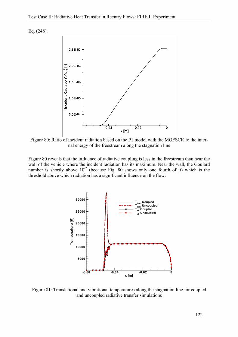
Abstract Radiative heat transfer is analyzed in rocket combustion chambers and in the flow around a re-entry vehicle. To do so, the governing equations of the P1 radiation transport model are derived, afterwards discretized using the Finite Volume Method and finally implemented in the CFD solver NSMB. For spectral integration, different models are combined with the P1 radiation model. For radiative heat transfer in rocket combustion chambers Weighted Sum of Gray Gases Models (WSGGM) are identified for spectral modeling and their governing equations with the P1 model are derived to implement them in NSMB. For radiative heat transfer in re-entry flows, a spectral model is developed based on a Full Spectrum k-Distribution (FSK) using the spectral database PARADE. The model is applicable to nonhomogeneous media with varying temperature and mole fractions. The governing equations of the P1 model in conjunction with this model are derived and the model is also implemented in NSMB. All models for radiative heat transfer are validated in several one-dimensional cases and show good agreement with analytical solutions. The sole P1 model yields an error below 5 %. The combination of the P1 model and the WSGGM gives satisfactory results. The FSK reproduces nearly exact results with errors below 1 % for homogeneous media. For nonhomogeneous media, the Multi Group Full Spectrum Correlated k-Distribution (MGFSCK) reduces devia-tions of the FSK from over 250 % to below 10 %. Radiative transfer in rocket combustion chambers is analyzed using the P1 model and several WSGGM for H2/O2 and CH4/O2 combustion. The results reveal that simple WSGG models yield nearly the same radiative wall heat flux (RWHF) with less computational efforts than more complex WSGGM. Using WSGGM appropriate for nonhomogeneous media decreases the RWHF. An enlarged chamber volume increases the RWHF. The influence of radiation on the flow is investigated in a loosely coupled simulation, revealing a negligible effect. For CH4/O2 combustion the maximum relative RWHF decreases compared to H2/O2 combustion. The maximum local ratio of the RWHF and total wall heat flux (TWHF) is between 8-10 % near the injector face plate while the integrated ratio is below 3 % for both propellant combi-nations. The analysis reveals a small influence of radiation on the heat loads in the combus-tion chambers investigated. The second system analyzed is the re-entry of the FIRE II capsule. Several models in NSMB for the simulation of the flow are improved and tested. With a final set of models, the convec-tive wall heat flux (CWHF) as well as the temperature and species number densities lie within 10 % deviation compared to former numerical investigations of the FIREII flight test. A one-dimensional Line-by-Line (LBL) radiative heat transfer analysis along the stagnation line is done afterwards with PARADE. The deviation of this analysis is below 2% in terms of RWHF at the stagnation point with regard to the flight experiment. The P1 model with the MGFSCK yields good accuracy compared to the LBL results with a reduction in computational effort by a factor of nearly 1000. Concerning RWHF at the stagna-tion point, the error is around 20 %. Concerning divergence of radiative heat flux the error is lower than 30 % over most of the stagnation line. The divergence of radiative heat flux predicted by the P1 model with the MGFSCK for the entire domain is coupled in the total energy equation of NSMB to examine the influence of radiation on the flow. It reveals that the CWHF decreases by a maximum of 10 % and the flow properties do not change by more than 5 %. This concludes a minor influence of radia-tion on the flow for the chosen trajectory point of the FIREII flight test.

Zusammenfassung Der Wärmeübergang durch Strahlung wird in Raketenbrennkammern und in der Strömung um einen Wiedereintrittskörper untersucht. Dazu werden die Gleichungen des P1 Strahlungs-transportmodells mit Hilfe der Methode der Finiten Volumina diskretisiert und in den CFD Löser NSMB implementiert. Zur spektralen Integration werden verschiedene Modelle mit dem P1 Modell kombiniert: Für den Strahlungswärmetransport in Raketenbrennkammern werden geeignete Weighted Sum of Gray Gases Modelle (WSGGM) mit dem P1 Modell ge-koppelt und in NSMB eingebaut. Für den Strahlungswärmetransport in Wiedereintrittsströ-mungen wird ein eigenes Spektralmodell auf Basis der Full Spectrum k-Distribution (FSK) entwickelt und in NSMB implementiert. Alle Strahlungsmodelle werden anhand eindimensionaler Fälle validiert und ergeben eine gute Übereinstimmung mit den analytischen Lösungen. Das P1 Modell weist Abweichungen von unter 5 % auf und auch die Kombination aus P1 Modell und WSGGM ergibt gute Resul-tate. Das FSK Modell reproduziert die nahezu exakten Ergebnisse für homogene Medien mit einem Fehler von weniger als 1 %. Für inhomogene Medien reduziert die Multi Group Full Spectrum Correlated k-Distribution (MGFSCK) die Abweichungen des FSK von über 250 % auf weniger als 10 %. Der Strahlungstransfer in Raketenbrennkammern wird mit dem P1 Modell und mehreren WSGGM für H2/O2 und CH4/O2 Verbrennung analysiert. Die Ergebnisse zeigen, dass einfa-che WSGGM mit weniger Rechenaufwand nahezu denselben Strahlungswandwärmestrom vorhersagen wie komplexere WSGGM. Die Verwendung von WSGGM für inhomogene Me-dien verringert den Strahlungswandwärmestrom, wohingegen eine Vergrößerung des Brenn-kammervolumens ihn erhöht. Der Einfluss der Strahlung auf die Strömung wird im Rahmen einer lose gekoppelten Simulation untersucht und ergibt einen geringen Effekt. In der CH4/O2 Verbrennung verringert sich der maximale relative Strahlungswandwärmestrom im Vergleich zur H2/O2 Verbrennung. Das maximale Verhältnis aus Strahlungswandwärmestrom zu kon-vektivem Wandwärmestrom liegt lokal zwischen 8 und 10 % nahe dem Injektor und integral bei unter 3 % für beide Brennstoffkombinationen. Die Untersuchung ergibt einen geringen Einfluss des Strahlungswandwärmestroms auf die Wärmelasten der Brennkammerwände. Das zweite untersuchte System ist der Wiedereintritt der FIRE II Kapsel in die Erdatmosphä-re. Zur Simulation der Strömung werden verschiedene Modelle in NSMB verbessert und ge-testet. Mit diesen Modellen liegen der konvektive Wandwärmestrom sowie die Temperatur und Teilchendichten nahe an den Ergebnissen voriger Simulationen des FIRE II Wiederein-tritts, mit Abweichungen von unter 10 %. Der Strahlungswärmetransport wird zunächst eindimensional entlang der Staupunktstromlinie mit Hilfe von sehr genauen Line-by-Line (LBL) Spektraldaten untersucht. Die Abweichung des Strahlungswandwärmestroms am Staupunkt zu den Ergebnissen des realen Wiedereintritts beträgt weniger als 2 %. Die Kombination aus P1 Modell und MGFSCK liefert gute Ergeb-nisse im Vergleich zur LBL Untersuchung, bei einer Verringerung des Rechenaufwandes um nahezu den Faktor 1000. Die Abweichung des Strahlungswandwärmestroms zur LBL Rech-nung beträgt ca. 20 %, während die Divergenz des Strahlungswärmestroms im Feld größten-teils Abweichungen von unter 30 % aufweist. Die Divergenz des Strahlungswärmestroms, basierend auf dem P1 Modell und dem MGFSCK, wird in die Erhaltungsgleichung der Totalenergie in NSMB gekoppelt. Dies ver-ringert den konvektiven Wandwärmestrom um 10 % und verändert die Strömungsgrößen um weniger als 5 %, was einen geringen Einfluss der Strahlung auf die Strömung für den gewähl-ten Punkt der FIRE II Wiedereintrittstrajektorie ergibt.

Table of Contents

VII

Table of Contents Table of Contents ....................................................................................................................VII Nomenclature ........................................................................................................................... IX 1. Introduction ........................................................................................................................ 1

1.1. Motivation .................................................................................................................. 1 1.2. Literature Survey........................................................................................................ 6 1.3. Objectives of this work ............................................................................................ 11

1.3.1. Implementation and Validation Work for Radiative Heat Transfer Analysis.. 12 1.3.2. Test Case I: Radiative Heat Transfer in Modern Rocket Combustion Chambers 12 1.3.3. Test Case II: Radiative Heat Transfer for the FIRE II Re-Entry ..................... 12

2. Governing Equations of Fluid Dynamics for Hypersonic Re-Entry Flows ..................... 13 2.1. The Conservation Equations of Fluid Dynamics ..................................................... 19

2.1.1. Transport Properties ......................................................................................... 21 2.1.2. Source Terms.................................................................................................... 23

3. Governing Equations of Radiative Transfer in Participating Media................................ 27 3.1. The Radiative Transfer Equation ............................................................................. 27 3.2. Transport Modeling: The P1 Radiation Model ........................................................ 28 3.3. Spectral Modeling: The Weighted Sum of Gray Gases Model................................ 37

3.3.1. The P1 Radiation Model in Conjunction with the WSGGM ........................... 38 3.3.2. The WSGGM for Homogeneous Media .......................................................... 41 3.3.3. Spectral Modeling in Nonhomogeneous Media............................................... 43 3.3.4. The WSGGM for Nonhomogeneous Media .................................................... 43 3.3.5. The WSGGM for Mixtures .............................................................................. 47

3.4. Spectral Modeling: The Full Spectrum k-Distribution Method based on Spectral Data from PARADE............................................................................................................. 49

3.4.1. The Plasma Radiation Database PARADE...................................................... 50 3.4.2. The P1 Radiation Model in Conjunction with the Full Spectrum k-Distribution Method in Homogeneous Media ...................................................................................... 51 3.4.3. The P1 Radiation Model in Conjunction with the Full Spectrum Correlated k-Distribution Method in Nonhomogeneous Media............................................................ 55

4. Implementation of the P1 Radiation Model in NSMB..................................................... 61 4.1. Finite Volume Approximation of the P1 Radiation Model...................................... 61 4.2. Validation of the P1 Radiation Model...................................................................... 69

5. Implementation of the Weighted Sum of Gray Gases Model in NSMB.......................... 72 5.1. Validation of the P1 Radiation Model combined with the WSGGM ...................... 72

6. Implementation of the Full Spectrum k-Distribution Method in NSMB......................... 74 6.1. Validation of the P1 Radiation Model combined with the Full Spectrum k-Distribution........................................................................................................................... 74

7. Summary of Implementation Work.................................................................................. 79 8. Test Case I: Radiative Heat Transfer in Modern Rocket Combustion Chambers ........... 81

8.1. Results for the Flow Field ........................................................................................ 81 8.2. Investigation of Radiative Heat Transfer ................................................................. 83

8.2.1. Determination of the Combustion Chamber Emissivity .................................. 84 8.2.2. Radiative Heat Transfer Analysis for H2/O2 combustion................................. 86 8.2.3. Radiative Heat Transfer Analysis for CH4/O2 combustion.............................. 95 8.2.4. Comparison to former investigations of the Space Shuttle Main Engine Main Combustion Chamber..................................................................................................... 100

Table of Contents

VIII

9. Test Case II: Radiative Heat Transfer in Reentry Flows: FIRE II Experiment ............. 104 9.1. CFD Simulation of the FIRE II Flight Experiment at 1636 seconds ..................... 105

9.1.1. Mesh Generation ............................................................................................ 105 9.1.2. Results for the Flow Field .............................................................................. 106

9.2. Simulation of Radiative Heat Transfer for the FIRE II Experiment at 1636 seconds 115

9.2.1. One-Dimensional Line-by-Line Radiative Heat Transfer Analysis............... 115 9.2.2. Radiative Heat Transfer Analysis using the P1 Model and the MGFSCK .... 118 9.2.3. Investigation of Radiation Coupling .............................................................. 121

10. Summary and Conclusion .......................................................................................... 125 10.1. Summary of Results ........................................................................................... 125 10.2. Conclusion.......................................................................................................... 126 10.3. Further Study...................................................................................................... 127

List of Figures ........................................................................................................................ 129 List of Tables.......................................................................................................................... 133 Appendix ................................................................................................................................ 134

A. Coefficients for Blottner’s model............................................................................... 134 B. Coefficients for Gupta & Yos’ model ........................................................................ 134 C. Coefficients for Park’s model .................................................................................... 141 D. CEA Coefficients ....................................................................................................... 144

Bibliography........................................................................................................................... 146

Nomenclature

IX

Nomenclature Latin Symbols: a [1 m ] Absorption coefficient [ ] Polynomial coefficient [ ] Exponent for vibrational-dissociation coupling A [ ] Polynomial coefficient [ ] Symbol for chemical species [ 2m ] Surface

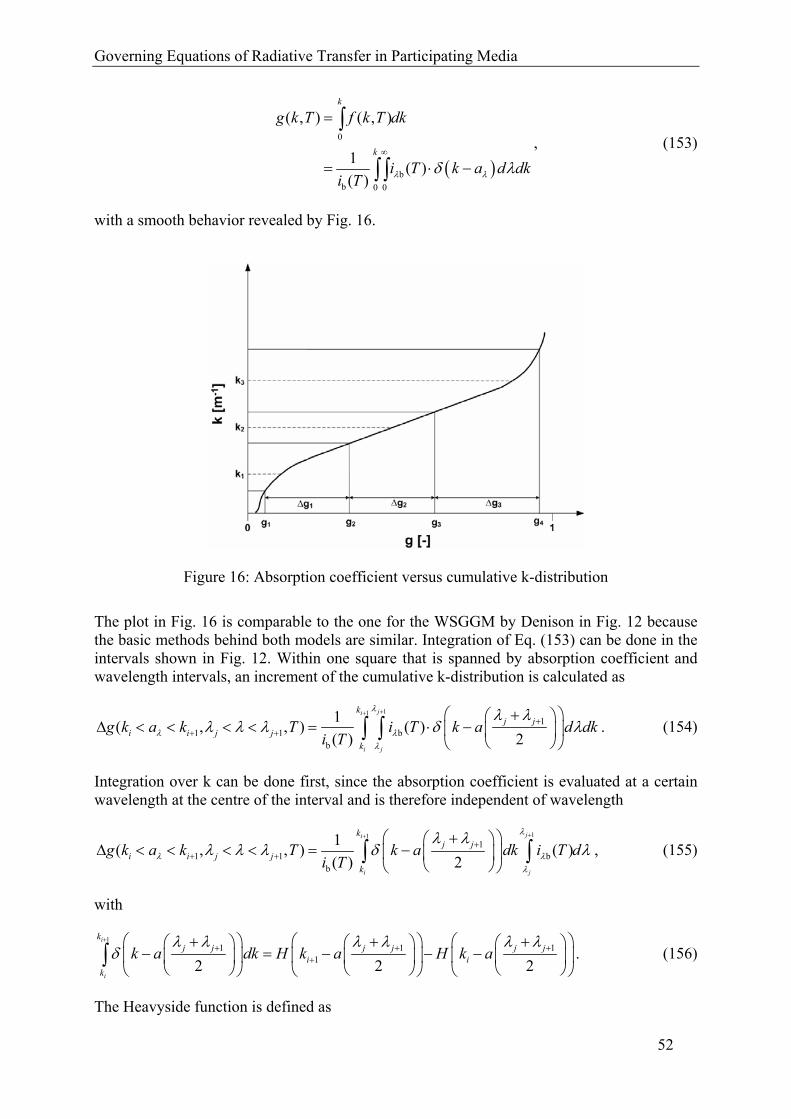
A

[ 2m ] Surface vector b [ ] Polynomial coefficient [ ] Exponent for vibrational-dissociation coupling B [ ] Polynomial coefficient c [ ] Abbreviation for cosinus

0c [ m s ] Speed of light

pc [ J kg K ] Specific heat capacity at constant pressure

Vc [ J kg K ] Specific heat capacity at constant volume

C [ ] Charge [ ] Polynomial Coefficient

absC [ 2m mol ] Absorption cross section

absC [ 2m mol ] Mean absorption cross section

D [ 2m s ] Diffusion coefficient [ ] Polynomial coefficient Da [-] Damköhler Number e [ 2W m ] Radiation power E [ ] Polynomial Coefficient [ J kg ] Energy [ K ] Arrhenius’ Activation Temperature f [ ] Arbitrary function

[ ] Probability density function for FSK Model [ ] Fluxes in x-direction F [ ] Blackbody distribution function g [ ] Cumulative k-distribution [ ] Fluxes in y-direction g [ ] Mean cumulative k-distribution

G [ 2W m ] Incident radiation [ ] Arbitrary function i [ 2W m sr ] Radiation intensity I [ ] Number of gray gases H [ ] Heavyside function h [ J kg ] Specific enthalpy [ ] Fluxes in y-direction [ J s ] Planck’s constant j [ 2kg m s ] Diffusion flux J [ ] Number of intervals for one gray gas

Nomenclature

X

[ ] Order of polynomial for WSGGM [ 2W m ] Radiosity

[ 3mol m s ] Chemical net production rate

k [ J K ] Boltzmann constant

[1 m ] Reordered absorption coefficient for FSK

[ W K m ] Thermal conductivity

[ 1-ν3 1mol m s ] Reaction rate

[ ] Factor for modified Marshak boundary condition K [ ] Number of species

[ b aν -ν3mol m ] Equilibrium constant

Kn [ ] Knudsen number l [ ] Summation index [ ] Legendre polynomial index L [ m ] Characteristic length Le [ ] Lewis number m [ ] Summation index [ ] Legendre polynomial index M [ kg mol ] Molar mass n [ ] Summation index [ ] Refractive index [ ] Constant for modified Marshak boundary

condition n

[ ] Unit surface vector N [ ] Order of Spherical Harmonics [ 31 m ] Number density o [ ] Summation index p [ 2N m ] Pressure

[ ] Summation index

FP [ ] Polynomial function for blackbody distribution

function P [ ] Legendre polynomial q [ 2W m ] Heat flux [ ] Summation index q

[ 2W m ] Heat flux vector r [ m ] Radius [ ] Mixture ratio r

[ m ] Spatial vector R [ ] Residual

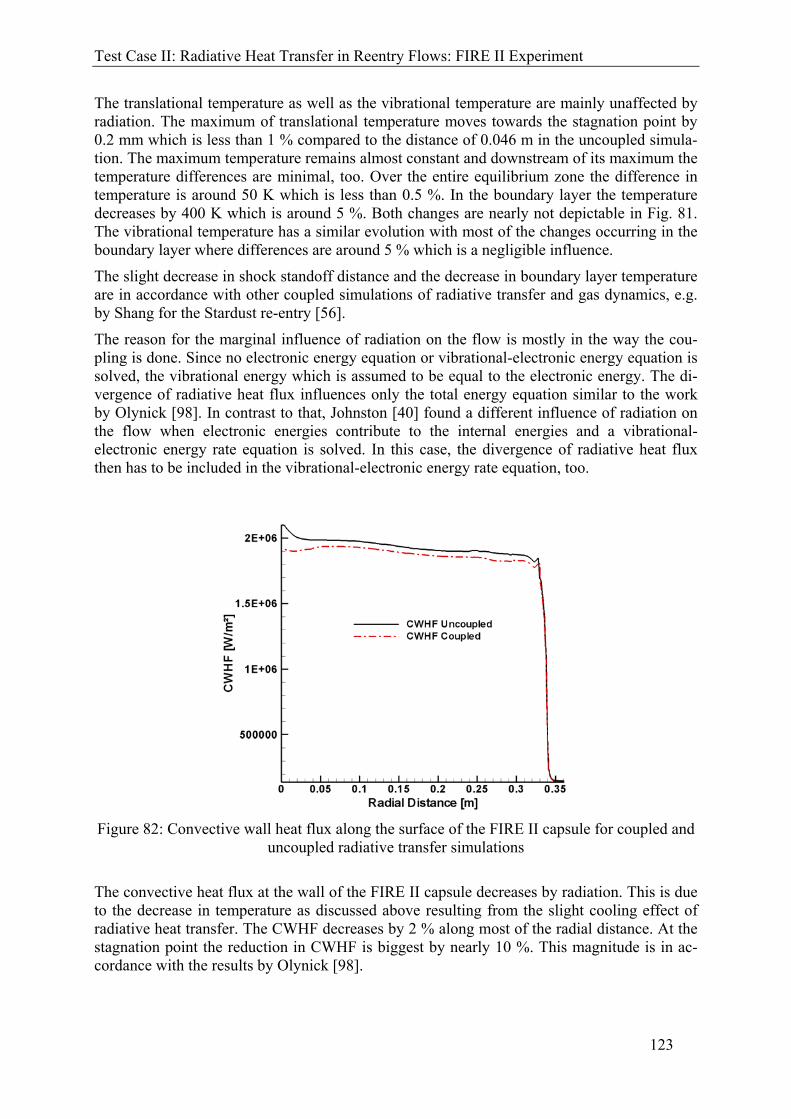
[ J kg K ] Gas constant 0R [ J mol K ] Universal gas constant

s [ m ] Direction [ J kg K ] Entropy [ ] Abbreviation for sinus s

[ ] Directional vector S [ m ] Path / Path length

Nomenclature

XI

[ 3W m ] Radiative source term [ ] Source term vector t [ s ] Time T [ K ] Static temperature u [ m s ] Velocity

u

U v

w

[ m s ] Velocity vector

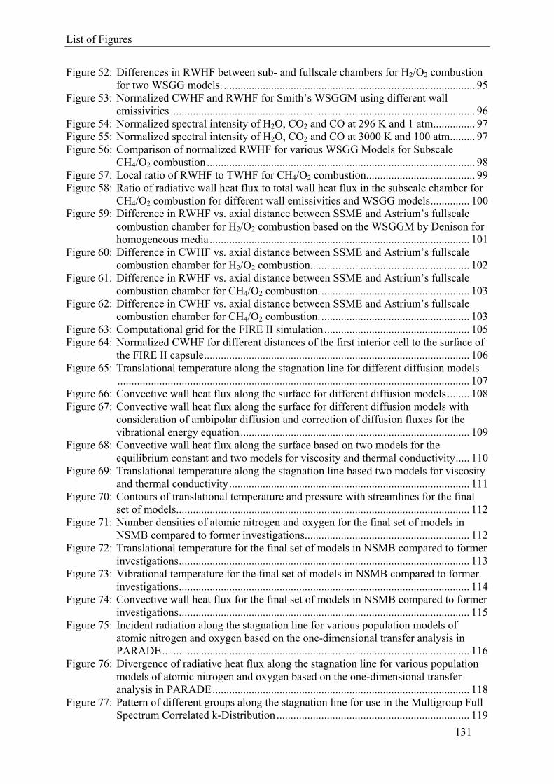
V [ 3m ] Volume w [ ] Blackbody weight W State vector x [ m ] x-coordinate X [ ] Molar fraction y [ m ] y-coordinate Y [ ] Mass fraction

mlY [ ] Spherical Harmonics

z [ m ] z-coordinate Z [ ] Temperature ratio [ ] Target function Greek Symbols: [ ] Arrhenius exponent

1 [ m s ] Property for diffusion coefficient according to Gupta

ji [ m ] Wavelength interval

[ ] Dirac function [ ] Emissivity [ 3W m ] Emission coefficient [ ] Curve linear space [ ] Curve linear space [ ] Polar angle [ K ] Characteristic Temperature [ m ] Wavelength

[ m ] Mean free path [ kg m s ] Dynamic viscosity [ ] Stoichiometric coefficient [ ] Logarithm of absorption cross section

[ kg mol ] Mean Molar Mass [ ] Logarithmic absorption cross section [ ] Curve linear space

/b sb [ ] Broadening/self broadening parameter

[ 3kg m ] Density

[1 m ] Scattering coefficient

[ 2 4W m K ] Stefan- Boltzmann constant [ ] Optical thickness

Nomenclature

XII

[ s ] Relaxation time [ 2kg m s ] Viscous stress tensor [ ] Scattering phase function [ ] Property of Wilke’s mixing rule Thermodynamic state vector [ ] Logarithm of elevated pressure [ ] Azimuthal angle [ ] Arbitrary property [ sr ] Solid angle [ 3kg m s ] Mass source term

[ J kg s ] Vibrational energy source term 1,1 [ 2m ] Collisional cross section for diffusion coefficient

Subscripts: 1 First interior cell abs Absorption avg Average b Blackbody Boundary cell Backwards c Concentration based Carbon dioxide e Electron f Formation Forward fluid Fluid cell g Gas Descriptor for g-space in FSK model ghost Ghost cell group Property of each group i Index of direction Index of cell face Index of species I Index of cell centre init Initialization j Index of species J Index of cell centre k Index of species Thermal conductivity Index of reactions Descriptor for k-space in FSK model K Index of cell centre l Numeration index lower Lower interval m Medium Molecule max Maximum min Minimum

Nomenclature

XIII

n Numeration index Iteration index p Pressure based rad Radiation ref Reference state rot Rotational s Species t Total property trans Translational upper Upper interval v Viscous fluxes w Wall Water x X-direction y Y-direction z Z-direction Polar angle Spectral value Azimuthal angle 0 Clear gas property 3 Based on 3 gray gases 10 Based on 10 gray gases Superscripts: a Reactants b Products j Index for gray gas interval lower Lower boundary of gray gas interval m Numeration index n Time level upper Upper boundary of gray gas interval vib Vibrational x Component of vector in x-direction y Component of vector in y-direction z Component of vector in z-direction ', '', ''' Polynomial coefficient designator * Correlated value Abbreviations and Acronyms: ATV Automated Transfer Vehicle CFD Computational Fluid Dynamics CWHF Convective Wall Heat Flux DOM Discrete Ordinates Method DPLR Data-Parallel Line Relaxation DSMC Direct Simulation Monte Carlo DTM Discrete Transfer Model FIRE Flight Investigation of Reentry Environment FS(C)K Full Spectrum (Correlated) k-Distribution FUN3D Fully Unstructured Navier Stokes 3D

Nomenclature

XIV

FVM Finite Volume Method HIFIRE Hypersonic International Flight Research

Experimentation HyShot Hypersonic Shot ICBM Intercontinental Ballistic Missiles LAURA Langley Aerothermodynamics Upwind Relaxation Algorithm LEMANS “Le” Michigan Aerothermodynamics Navier-

Stokes Solver LEO Low Earth Orbit LORAN Langley Optimized Radiative Nonequilibrium LBL Line-by-Line LU-SGS Lower-upper Symmetric Gauss Seidel MCC Main Combustion Chamber MDA Modified Differential Approximation MGFSCK Multi Group Full Spectrum Correlated k-

Distribution NASA National Aeronautics and Space Administration NEQAIR Nonequilibrium Air Radiation NSMB Navier Stokes Multiblock Solver PARADE Plasma Radiation Database PDF Probability Density Function QSS Quasi Steady State RTE Radiative Transfer Equation RWHF Radiative Wall Heat Flux SETI Search for Extraterrestrial Intelligence SLMB Spectral Line Moment Based SLW Spectral Line Weighted Sum of Gray Gases

Model SSME Space Shuttle Main Engine TWHF Total Wall Heat Flux VUV Vacuum Ultra-Violet WSGGM Weighted Sum of Gray Gases Model

Introduction

1

1. Introduction 1.1. Motivation

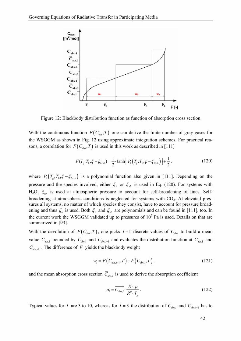
The investigation of heat transfer is crucial in many fields of aerospace engineering. For criti-cal systems an analysis has to be performed to assure that the heating limits of the system are not exceeded by internal or external heat loads. Besides convection and conduction, radiation is the third mechanism of heat transfer. In contrast to the other two, radiative heat transfer is independent on a propagation medium due to its electromagnetic origin [1, p.2]. This makes radiative heat transfer more complex than for example the analysis of convective heating .Radiation can propagate in all directions even without a medium, e.g. in outer space where the lack of air prevents convective heat transfer.

The analysis of radiative heat transfer is important in various aerospace applications, for ex-ample in the thermal management of satellites or spacecrafts. Radiation from the sun is ab-sorbed by the surface of the satellite or spacecraft. Depending on the fourth power of the sur-face’s temperature, it emits radiation back into space [2, p.19]. In combination with other ef-fects (e.g. heating through electronic components), the satellite or spacecraft experiences a net gain or loss of energy which might have an influence on its mission lifetime. For example, any loss of energy has to be compensated by heating mechanisms which will possibly use up the limited fuel of the satellite or spacecraft.

Other systems influenced by radiative heat transfer are those at high temperatures, e.g. com-bustion chambers or re-entry flows. In these systems, radiative heat transfer occurs in partici-pating media, for example in gases. The emission of the medium depends on its fourth power [2, p.19], underlining the importance of radiative heat transfer in systems with high tempera-tures. In participating media modeling of radiative heat transfer is complicated because the absorption- and emission-characteristics are subject to quantum physics and add a spectral dependency to the radiative heat transfer because they vary strongly over wavelength [1, p. 303]. More details on the nature of radiation are given later in this work and are covered by several textbooks, like the ones by Modest [1] or Siegel [2].

In some cases radiation can also influence the momentum of objects, for example when using solar sails for space propulsion. In case a photon is reflected by a surface, its momentum is transferred to the surface [3]. According to Newton’s second law the change of momentum results in a force which adds to other external forces and propels a spacecraft if it is properly aligned to the sun. The order of magnitude of this additional force depends on the radiation pressure at a given distance from the sun and the sail’s area. Since the radiation pressure at Sun-Earth distance is in the order of 10-5 Pa [3], the solar sails have to have a large area in order to produce a significant force for interstellar travel.

Introduction

2

Figure 1: Artist’s conception of a spacecraft powered by a solar sail [4]

Besides by reflection of solar photons, the momentum of spacecrafts can also be changed by their own thermal emission. Most recently, the Pioneer anomaly [5] was very likely solved by taking into account the effect of radiation on the momentum of the Pioneer space probes. In a detailed thermal analysis, Turyshev et al. [6] found that anisotropic thermal emission from the Pioneer spacecrafts resulted in an additional force on the spacecrafts, slowing them down more than expected.

Nevertheless, in this work radiation shall be treated only as a means of heat transfer, neglect-ing any influence on the momentum. Radiative heat transfer is analyzed in modern rocket combustion chambers as well as in the flow around a re-entry vehicle entering earth’s atmos-phere, representing two prominent high enthalpy systems. Since enthalpy consists of both internal and kinetic energy, high enthalpy systems can either be systems at high internal en-ergy, respectively at a high temperature, or systems at high kinetic energy, respectively at a high velocity.

Rocket combustion chambers are high enthalpy systems due to their combustion temperatures which can easily exceed 3000 K [7, p. 40]. In the combustion process, fuel and oxidizer enter the combustion chamber and react exothermally, thereby transferring chemical energy into thermal energy. Through expansion in the nozzle of the rocket engine the internal energy is then converted into kinetic energy which finally produces thrust. Radiative heat transfer in rocket combustion chambers has long been used only for cooling purposes in the nozzles of rocket engines [7, p.270]. For that, one uses the fact that the hot structure, e.g. the nozzle of the engine, emits radiation proportional to its temperature’s fourth power. If the nozzle is in outer space with a temperature of around 1000 K, radiating against the cold space at 3 K, the surface radiative heat transfer is in the order of 104 W/m² based on the Stefan-Boltzmann law [2, p.19]. Currently, radiation is used as cooling mechanism for some upper stage engines, like SpaceX’s Merlin engine [8]. Figure 2 shows the glowing nozzle during a Falcon 9 test flight.

Introduction

3

Figure 2: Radiation cooled Merlin upper stage rocket motor on a Falcon 9 test flight [9]

Another aspect of radiative heat transfer in rocket motors is plume radiation [7, p.319] in which the emission of the exhaust gas is important. On the one hand this emission heats the base of the rocket, posing a problem to the insulation of the rocket and its fuel tanks. Recent investigation on radiative heat transfer through plume emission from solid rocket motors has been done e.g. for the European launcher Vega [10]. Secondly, especially for military applica-tions, plume emission can be a reconnaissance issue as it helps localizing the rocket or aircraft as the origin of the emission. Analysis in this field compasses the investigation of infrared emission from plumes e.g. for state-of-the-art turbojet engines [11, 12].

On the contrary, the influence of radiative heat transfer on the heat loads inside the combus-tion chamber is often neglected even though temperatures are high enough to cause emission in the order of 105 W/m² and beyond based on the Stefan-Boltzmann law [2, p.19]. Sutton [7, p. 319] states that radiative heat loads can contribute up to 40 % to the entire heat loads. In-vestigations of radiative heat loads on the Space Shuttle Main Engine (SSME) Main Combus-tion Chamber (MCC) by several authors indicated a significant influence of radiation on the total heating [13, 14, 15, 16].

In the other part of this work, the flow around a re-entry capsule is investigated. The re-entry flow is a high enthalpy system due to its velocity. Even the lowest orbital velocity for space-crafts re-entering Earth’s atmosphere is in the order of 8 km/s which gives a specific kinetic energy of around 32·106 J/kg. At these conditions a compression shock occurs, triggering sev-eral effects in the flow like chemical reactions or internal energy transitions. In the early ages of aerothermodynamics, the compression shock posed a problem when re-entry vehicles were designed according to supersonic theory: slender bodies with a sharp nose producing an oblique shock [17, p.17]. Unfortunately, the oblique shock lay very close to the tip of the nose, as the upper left image of Fig. 3 shows. There, it interfered with the boundary layer of the vehicle in a shock-boundary-layer-interaction, characterized by an increase of heat trans-fer [18, p.530].

Introduction

4

Figure 3: Shadowgraph images of different capsule shapes [19]

During the design of Intercontinental Ballistic Missiles (ICBM) these high heat loads posed a problem since they demanded either efficient active cooling mechanisms or great heat sinks which literally “soaked” the heat loads. Both methods increased the mass of the ICBM dra-matically while at the same time decreasing its range [17, p.22]. The solution to this problem was the so called blunt body. With a blunted nose, the compression shock moves upstream to become a detached shock as seen on the right upper side of Fig. 3. The blunter the nose, the greater the deflection of the flow around the vehicle is, preventing shock-boundary layer in-teraction and thus reducing the heat loads on the structure significantly. Detached shock waves are not limited to re-entry flows. Figure 4 shows Zeta Ophiuchi in the stellar constella-tion Ophiuchus. The star moves at a velocity of 24 km/s [20] producing a detached bow shock of interstellar matter.

Figure 4: Interstellar bow shock caused by the movement of the star Zeta Ophiuchi [20]

Introduction

5

For re-entry flows, convective and radiative heating have an inverse dependency. The convec-tive heating is inversely proportional to the square root of the vehicle’s nose radius while the radiative heating is directly proportional to the vehicle’s nose radius [18, p.272]. This leads to competitive design objectives because the bigger the nose radius, the more the flow is de-flected around the vehicle decreasing the convective heat load but at the same time increasing the radiative heating.

Similar to the rocket motors, one of the biggest applications of radiative heat transfer for re-entry vehicles is concerning cooling. Various systems, from which the most prominent one was the now-retired Space Shuttle [21, p. 41], use radiation cooling to keep the temperature of the system’s outer skin below critical values. If the re-entry occurs at a certain shallow flight path angle, there is sufficient time for the radiative heat transfer to equilibrate the convective heating, becoming an efficient cooling mechanism.

Besides cooling issues, the investigation of radiative heat transfer as a contributor to the heat loads during re-entry has a long legacy reaching back to the 1960’s. During the first years of the Apollo project, engineers had little knowledge about the radiative and convective heat loads during re-entries from lunar trajectories. The predecessors of the Apollo program, the Mercury and Gemini programs had sub-orbital or orbital speeds below 8 km/s, so the need arose to gather data for re-entries in excess of 11 km/s [22]. This led to project FIRE (Flight Investigation Reentry Environment) with test flights FIRE I and FIRE II.

Figure 5: NASA technicians working on FIRE capsule [30] (left) and FIRE II capsule before launch (right) [23]

FIRE I was launched on the 14th of April in 1964 [24] while FIRE II launched on the 22nd of May in 1965 [25]. For both flights, the same capsule shape with a diameter of 0.67 m was used as shown in Fig. 5 [26], mounted on top of an Atlas D rocket. Both flight tests had the objective to measure total and radiative heating rates when entering the atmosphere at 11.3 km/s at an altitude of 121920 meters (400000 feet). For this, they were equipped with radi-ometers and thermocouples [27, 26]. Details on the trajectory and the timeline of events are given in [24] for FIRE I and in [25] for FIRE II.

To endure the enormous heat loads during re-entry, the gauges were shielded. To avoid abla-tive heat shields, whose ablation products would have interfered with the radiometer meas-urements [28], the thermocouples and radiometers were arranged in three layers from which

Introduction

6

each was shielded by Beryllium [29, p.2]. During re-entry, the Beryllium layer melted and the underlying phenolic-asbetos heat shield was ejected to expose the next Beryllium layer with a new set of thermocouples and radiometers [29, p. 2]. The left side of Fig. 5 shows the ejectable heat shields being added to the FIRE capsule in a wind tunnel at NASA Langley in 1962 [30].

The FIRE I flight test in 1964 performed generally well but experienced minor issues with a sudden change in yaw rate [24, p.7] and a deterioration in the telemetry signal [24, p. 9]. The cause of the former issue could not be cleared in detailed although some researchers suspected some kind of collision of the capsule with the upper stage of the Atlas D rocket [24, p. 8]. The latter issue was very likely caused by a broken connector in one of the antennas [24, p. 9] and led to a breakdown of telemetry transfer later in the re-entry.

To make sure the yaw rate issue had no influence on the data and to obtain a continuous te-lemetry transfer, the FIRE II experiment was launched in 1965 and performed flawlessly gathering all necessary data as expected. A collection of the data for convective and radiative heat flux for the FIRE II experiment can be found in [26, 31]. During peak heating, radiative heating was nearly 30 % of the total heating [32, p.39] but might have been even more be-cause the radiometers had a limited spectral resolution from 0.2µm-4.0µm [26, p.6], leaving out the strong so called vacuum ultra-violet (VUV) radiation below 0.2µm.

In total, one can say that radiation is the most complicate mode of heat transfer for which rea-son it is left out in many investigations. Nevertheless, it can have a significant impact in sys-tems like rocket combustion chambers and re-entry flows, giving the basic motivation to ana-lyze both in this work.

1.2. Literature Survey

The purpose of this chapter is to summarize the most important work of previous authors dealing with radiative heat transfer in high enthalpy systems. At first, literature concerning those two systems investigated herein, rocket combustion chambers and re-entry flows, is summarized. After that, literature dealing with the simulation of radiative heat transfer is re-viewed, focusing on radiation transport models and spectral models.

Concerning radiative heat transfer in liquid rocket combustion chambers, a good overview of previous work is given in the PhD thesis of Thellmann [16]. He summarized the work of sev-eral authors, all investigating radiative heat transfer in H2/O2 combustion chambers with the help of certain radiation transport models, mostly the Discrete Ordinates Methods (DOM) and spectral models like the Weighted Sum of Gray Gases Models (WSGGM).

Thellmann [16] himself did a CFD analysis of radiative heat transfer in the SSME MCC using different radiation transport models, among them the simple Rosseland Radiation Model, the P1 model and the Discrete Transfer Model (DTM). For spectral integration he used the WSGGM. Thellmann simulated the flow field in the SSME MCC using CFD methods. Based on that flow field, he found that the Radiative Wall Heat Flux (RWHF) in the SSME for tradi-tional H2/O2 combustion was on average 7.7 % of the Total Wall Heat Flux (TWHF). With a fictitious CH4/O2 combustion, assuring thrust identity to the H2/O2 combustion, the ratio in-creased to 8.8 %. The main shortcoming of his analysis was the prediction of the flow field which had not been validated against any experimental data for the SSME MCC because all of them were classified. As a substitute to experimental results, Thellmann compared the re-sults in both convective and radiative heating to former results by Wang [13] and Naraghi [14], thereby partially confirming their estimates for the ratio of RWHF to TWHF.

Additional work since then has been done for the analysis of radiative heat transfer in Scram-

Introduction

7

jet rocket combustion chambers by Crow and Boyd [33, 34]. They analyzed the HyShot II and HIFIRE-2 scramjets finding a negligible influence of radiative heat transfer on the total heat loads, with only 0.1-0.2 % of the total heating for the HyShot II experiment and around 1 % for the HIFIRE-2 scramjet caused by radiation. They used a one-dimensional DOM as radia-tion transport model and focused on H2O and OH as radiatively participating species using a narrow band spectral model. Their results have been partially confirmed by experimental analysis in the combustor of the HIFIRE-2 scramjet.

Research covering the investigation of radiative heat transfer in entry flows focuses on Earth re-entry as well as on entries on extraterrestrial planets or moons. For re-entry into Earth’s atmosphere, the FIRE II flight test and the re-entry of the Stardust sample return capsule are the most prominent cases investigated.

For FIRE II, early work on radiative heat transfer goes back to Hartung [35, 36]. Hartung de-veloped a Modified Differential Approximation (MDA) proposed by Modest [37] and a spec-tral database capable of dealing with Non-Boltzmanian energy level distributions. She imple-mented both in NASA’s radiation code LORAN. At that time, LORAN was the only code besides NEQAIR [38] that was able to account for Non-Boltzmanian electronic energy popu-lations in nonequilibrium radiation. Hartung investigated the FIRE II trajectory points at 1631, 1634 and 1637.5 seconds. The flow field was generated using NASA’s CFD code LAURA [39]. She found that with the MDA the radiative heating at the wall of the FIRE ve-hicle decreased by 25 % compared to simple one-dimensional transport models [35]. By tak-ing into account three different trajectory points, she was able to investigate the influence of nonequilibrium radiation on the radiative heating.

Johnston [40, 41] investigated the flow field of the FIRE II re-entry with a viscous shock layer approach while radiative heat transfer was determined using a one-dimensional transport model with line-by-line spectral integration based on a collisional radiative model. The colli-sional radiative model was able to deal with Non-Boltzmanian electronic energy state popula-tions, like NEQAIR or LORAN. The code was later named HARA by NASA. Johnston made uncoupled and fully coupled simulations of the flow field and the radiation field and found that the results of the coupled simulation matched the data of the FIRE II experiment best when applying a supercatalytic boundary condition.

Hash et al. [28] and Scalabrin [42, 43] focused on several trajectory points for the FIRE II re-entry but presented detailed results only for 1636 seconds. Hash et al. [28] compared different CFD codes concerning their flow field prediction and used NEQAIR for radiative heat trans-fer analysis, employing a one-dimensional transport model and LBL spectral integration. The different CFD codes compassed LAURA and DPLR, both by NASA and US3D by the Uni-versity of Minnesota. For DPLR they used two different versions, one in which the electronic modes of species are assumed to be in ground state and another in which a specific vibra-tional-electronic rate equation is solved. Details on the different assumptions are given later in this work. For the convective heating they performed a parameter study and found that diffu-sion mechanisms and grid accuracy had the biggest influence on the convective heating, fol-lowed by the electronic mode. Comparing all three CFD codes with a best-of set of models they discovered only small deviations of up to 11 % between all three codes in convective heating. In the radiative heat transfer analysis using NEQAIR they found that the electronic mode consideration had the biggest effect on the radiative heating. The results also matched the radiative heating of the FIRE II experiment at 1636 seconds within 10 %. Scalabrin [42, 43] developed a CFD code called LEMANS and compared the results of this CFD code in convective heating and flow properties to the results by Hash et al. The deviations in convec-tive heating to the results by LAURA were below 5 % at 1636 seconds. He also performed a one-dimensional radiative heat transfer analysis using LBL integration with NEQAIR. The

Introduction

8

radiative heating was slightly below the results of the flight experiment with a maximum error of 13 %.

Farbar and Boyd [44] used Direct Simulation Monte Carlo Methods (DSMC) for the flow field prediction at certain high-altitude trajectory points for which the continuum assumption is violated. They found good agreement with the flight test results with maximum deviations of 20 % but they did not consider radiative heat transfer in their work. Komives [45] analyzed radiative heat transfer for FIRE II at 1636 seconds with a one-dimensional model and LBL spectral integration based on a flow solution by the US Air Force Research Laboratory CFD code NH7air. His results in radiative heating at the wall overpredicted the flight experiment by a factor of 40 which was very likely caused by internal flaws in the radiation code.

Most recently, the FIRE II experiment was investigated by Wood [46], Andre [47], Sohn [58] and Savajano [50]. Wood [46] investigated the FIRE II re-entry under peak heating conditions at 1643 seconds using the unstructured CFD code FUN3D and the radiation code HARA by Johnston [40]. Based on the elements chosen for the unstructured mesh, the difference in con-vective heating was below 20 % compared to benchmark results by Johnston gained with LAURA [41]. Radiative heating results were within 6 % compared to Johnston’s results using line-by-line spectral integration in HARA.

Andre et al. [85] focused on the influence of different transport coefficients on the flow for FIRE II at 1634 seconds. They found that using Blottner’s model [48] for the viscosity yields less accurate results than using the model by Gupta & Yos [49]. Nevertheless, they did not state the influence of these models on the radiative heating.

Savajano et al. [50] predicted the flow field of FIRE II at 1634 seconds and 1643 seconds and simulated radiative heat transfer with a one-dimensional transport model and LBL spectral integration, thereby investigating the influence of Boltzmanian and Non-Boltzmanian energy level distributions on the radiative transfer. They found that considering Non-Boltzmanian energy level distributions at 1634 seconds significantly reduces the radiative heating. This effect was negligible at 1643 seconds because at this trajectory point the flow was nearly in chemical and thermal equilibrium, yielding equilibrium radiation and Boltzmanian energy level distributions.

For the Stardust sample return capsule [51], early work was done by Olynick [52] estimating the thermal loads on the capsule during re-entry for the design process of its thermal protec-tion system. Olynick used three different codes, GIANTS, NOVAR and FIAT to model the flow, radiation and thermal response of the capsule material and divided the entire re-entry trajectory into certain points. He focused on the modeling of ablation, including the effects of ablation products on the radiative heat transfer. He found that for the afterbody heat transfer the traditional design methods for the heat shield were not sufficient.

In the aftermath of the Stardust re-entry, several authors reproduced the flow conditions and investigated radiative heat transfer. Among them, Boyd [53] predicted the flow field at two different trajectory points, one at 81 km, the other at 71 km altitude using the continuum CFD code DPLR and a particle based DSMC code. The results for the flow field were imported into NEQAIR to simulate the LBL spectrum along a line of sight, originating from various locations along the surface of the vehicle and ending in freestream. By this, Boyd reproduced the spectra measured by the instruments used in the re-entry observation campaign of Stardust [54]. When using DPLR, Boyd considered the electronic modes of species in ground state, similar to one of Hash’s options in the FIRE II investigation [28]. For 81 km altitude, the re-sults by DPLR and DSMC yielded a spectrum which compared well to the measured one whereas for 71 km DPLR yielded a flow field causing the spectrum closest to the measured spectra. Based on the measured and simulated spectra, Boyd was able to deduce spectra for

Introduction

9

the metallic components of the capsule glowing during the fiery re-entry. He showed that most of the measured metallic lines originated from the white paint of the capsule containing potassium and zinc. Similar to that, Zhong [55] investigated the spectra caused by sodium which occurred as an impurity of the TPS material in the flow. The number density of sodium was estimated with a DSMC method. Zhong invented a kinetic model for the excited states of sodium and found that the results agreed well with the measured spectra.

Shang and Surzhikov [56] performed closely coupled simulations of radiation and gas dynam-ics accounting for the influence of radiation on the flow. By investigating several trajectory points of the Stardust re-entry, they found that the coupling decreased the shock layer tem-perature and shock stand-off distance while at the same time increasing the temperature in the boundary layer. Feldick developed a one-dimensional radiation transport model using LBL spectral integration methods and coupled it to the CFD solver DPLR [57]. Performing closely coupled simulations of the Stardust capsule at 62 km altitudes revealed only small influence of radiation on the flow properties. Sohn [58] investigated coupling of radiation and gas dy-namics for the Stardust probe at the same altitude using a DSMC solver for the prediction of the flow field and a Photon Monte Carlo solver for the radiative heat transfer. By using both statistical methods, he ensured consistency between flow field simulation and radiative trans-fer simulation. The results show similar tendencies as the results by Feldick [57] for that alti-tude with a decrease in convective heating if radiation is coupled to the flow simulation and little changes in temperature. Recently, Liebhart et al. used the ESA funded database PA-RADE to simulate radiative heat transfer in the Stardust re-entry [59] using a one-dimensional transport model and LBL spectral integration with new sets for highly excited states of mo-lecular nitrogen.

For re-entry from low earth orbit (LEO), Boyd [61] simulated emission profiles around ESA’s Advanced Transfer Vehicle (ATV) at four different trajectory points using continuum CFD and particle tracking DSMC methods as a precursor to the 60 ATV re-entry observation cam-paign [60]. The simulation was done similar to the one for Stardust using NEQAIR for the emission spectra. Compared to the Stardust re-entry, the emission per solid angle was lower due to the lower re-entry velocity (7.6 km/ s as opposed to 12.6 km/s). Nevertheless, the di-rectionally integrated emission was estimated in the same order of magnitude as in the Star-dust re-entry due to the bigger dimensions of the ATV.

Besides Earth re-entry, several investigations cover entries on extraterrestrial planets like Mars and moons like Titan which orbits Saturn. Surzhikov and Shang investigated several Mars missions; among them the European ExoMars mission [62]. As with the Stardust re-entry, they coupled radiation and gas dynamics simulations and found that radiative heat transfer exceeds convective heat loads on the leeward side of the ExoMars capsule at 4.22 km/s velocity and a density of 6.9·10-9 kg/m3. Beck et al. confirmed these characteristics using the CFD code TINA and various radiation databases, amongst others PARADE [63]. They showed that the radiative heating at the base of the capsule was locally at least twice the con-vective heating there. They could also show that radiative heating was dominated by CO2 ra-diation. For the Mars Sample Return Obiter, Gromov and Surzhikov demonstrated that the base radiative heating is in the order of the convective heating there which is highly depend-ent on the catalycity of the orbiter's surface [64].

Radiative heat transfer for entry into Titan’s atmosphere has been executed for the Huygens probe. Mazoue et al. investigated radiative heat transfer for Huygens’ entry, finding a radia-tive heat flux exceeding the convective heating using various CFD codes and NEQAIR for radiative transport and LBL spectral integration [65]. They also investigated the influence of the changing atmospheric conditions on the heating rates, revealing that for some conditions the integrated radiative heating is nearly twice the convective heating. Johnston used his

Introduction

10

newly developed collisional radiative model, as mentioned above for the FIRE II re-entry, to simulate radiative heat transfer for the Huygens probe [40, 66].Special attention was given to the modeling of CN radiation with the collisional radiative model. Johnston found that radia-tion coupling reduced the convective and radiative heating at three peak heating trajectory points by 15 % and 20 %, respectively.

As a general overview, Perrin et al. recently summarized shock layer radiation mechanisms for various atmospheres and entry conditions [67] while Bultel et al. [68] focused on an over-view of the physico-chemical modeling of re-entry plasmas.

Following the literature survey for the test cases investigated in this work is a literature survey concerning radiation transport and spectral models.

The modeling of radiation transport is one key element for the accuracy of radiative heat transfer simulations. Besides the traditional models like one-dimensional models, the P1 model or the DOM, some new models have been developed from which one is the Half Mo-ment Method by Dubroca and Klar [69]. Its origin is similar to the P1 radiation model but uses entropy minimization as closure condition. The P1 model and the DTM, which is a hy-brid of DOM and ray tracing, have been used by Thellmann for the investigation of radiative transfer in the SSME MCC [16]. Statistical DSMC methods are used extensively for radiation transport in mainly all systems. Karl used them for radiative heat transfer in re-entry flows [70] as well as Farbar [44], both for the analysis of the FIRE II experiment. Wang and Modest used the DSMC method for radiative heat transfer analyses with turbulence radiation interac-tion [71, 72] while in recent years Feldick, Ozawa and Modest developed several Monte Carlo methods for radiative heat transfer in re-entry systems [73, 74, 75].

The spectral modeling of radiative heat transfer has been thoroughly investigated in the last years in order to reduce the computational efforts of spectral integration. Especially in the radiative heat transfer analysis of re-entry flows, costly LBL analyses are often performed, e.g. for the FIRE II flight test [28, 42, 35, 36, 41, 50]. Within LBL analyses, the total number of transfer equations can easily be in the order of 104 e.g. for pure H2O flows [76]. To reduce these efforts, spectral models are used. The basic idea behind these models is to combine sev-eral lines in the spectrum having a similar behavior. Depending on the spectral range investi-gated, Narrow Band Models, Wide Band Models or Global Models can be used [1, p.306-307]. While the first two focus on a certain limited spectral range, Global Models can be used for radiative heat transfer in the entire spectrum. Furthermore both Narrow Band Models and Wide Band Models are not well suited for use in nonhomogeneous media [1, p.307]. In this work, Global Models are used because the range of the investigated spectra is too big to use Narrow Band or Wide Band Models effectively. For example the spectrum of pure H2O at conditions with temperatures of 3000K and a pressure of 1·107 Pa features over 27000 lines [76] rendering the use of Narrow Band or Wide Band Models inappropriate. The number of lines can be even higher, taking into account even more species at higher temperature like in the re-entry flows. Among the Global Models, the most prominent ones for the analysis of the entire spectrum are the Full Spectrum k-Distribution (FSK) and the WSGGM.

The FSK bases on the k-distribution method introduced by Goody [77] and was originally developed by Modest and Zhang [78]. According to Modest [1, p.617] the FSK is the exact version of the WSGGM. The main difference between the FSK and the k-distribution by Goody is that the former can be applied to the entire spectrum. The FSK is exact if the me-dium of radiative heat transfer is homogeneous. For nonhomogeneous media, Fu and Liou [79] described the method of correlated k-distributions. Modest and Zhang [80] applied the correlated k-distribution to the entire spectrum calling it the Full Spectrum Correlated k-distribution (FSCK). The FSCK has been used for radiative heat transfer analyses in several combustion systems [81]. In order to improve the accuracy of the correlated k-distributions,

Introduction

11

Modest introduced the Multigroup FSCK (MGFSCK) [82] that has been applied e.g. to radia-tive heat transfer investigations in hypersonic flows [83] in which nonequilibrium radiation occurs.

Similar to the FSCK is the method of correlated fictitious gases introduced by Riviere et al. [84]. In this model, the entire spectrum is re-ordered taking into account the different energy level characteristics, therefore increasing the correlatedness of the approach but also the com-putational efforts in comparison to the MGFSCK. The Spectral Line Moment Based (SLMB) method by Andre [85] is another option to improve spectral modeling. All models have in common that they use a spectral database to deduce the properties for spectral modeling.

In contrast, the second class of global model, the Weighted Sum of Gray Gases Model is often developed based on optimization techniques without spectral databases. The WSGGM was originally developed by Hottel [86] to approximate the total emissivity of a gas column. Up to now, most WSGGM are developed as curve-fits on total emissivity data which makes them less profound with respect to quantum physics due to the lack of spectral databases. Some of the most prominent models are by Smith [87] and Copalle [88], while Johansson [89] devel-oped one of the most recent WSGGM. Denison and Webb [90] recognized the drawback of all WSGGM and developed the Spectral Line WSGGM (SLW) which uses a spectral database for the determination of WSGGM properties. Denison and Webb [91] applied the SLW also to nonhomogeneous media while Solovjov and Webb improved the SLW in recent years [92]. The WSGGM and SLW have most recently been used for the simulation of radiative heat transfer in rocket combustion chambers [16, 93]

1.3. Objectives of this work

Summarizing the above, very few analysis of radiative heat transfer is available for rocket combustion chambers and if it is, the simulation of the underlying flow field in the chamber is often not validated against any experimental results. Additionally, the rather complex Discrete Ordinates Method is used for radiation transport in most cases. For the combustion chambers, the aim of this work is therefore to perform an analysis based on validated results for the flow field, focusing on both H2/O2 combustion and CH4/O2 combustion. For that purpose, the P1 model is chosen for radiative transport because it gives a reasonable compromise between accuracy and effort. For spectral integration, the WSGGM has proven its worth in former in-vestigations and is therefore used in this work, too.

For radiative heat transfer in re-entry flows there is a great need for improvement concerning transport modeling as well as for optimization concerning spectral modeling in order to per-form radiative heat transfer with an acceptable amount of computational resources. Most of the former work has been done using one-dimensional models for radiation transport and LBL methods for spectral integration. In this work, the P1 model is employed as a transport model to account for radiative transfer in the entire flow field instead of only at the stagnation line. Besides that, Hartung found that the MDA, which is similar to the P1 model, reduces the ra-diative heating compared to one-dimensional models [35]. To reduce computational efforts associated with spectral integration, the MGFSCK is used to develop a similar spectral model which promises to reduce the computational efforts for spectral integration by a factor of at least 10³ compared to LBL integration.

The analysis of radiative heat transfer in re-entry flows is often done with a different code than the analysis of the flow field. In this work, the radiation transport and spectral models are implemented in the CFD code NSMB which is also used to predict the flow field during re-entry. Using the same code for both phenomena makes any interface obsolete and eases the implementation work as one can rely on a proven structure of the code. The FIRE II re-entry

Introduction

12

at 1636 seconds is then chosen as a test case because it is one of the best documented projects and has been thoroughly investigated by various authors before providing a reliable database for comparison.

1.3.1. Implementation and Validation Work for Radiative Heat Transfer Analysis

To enable radiative heat transfer, the P1 radiation model is chosen for transport and is imple-mented in the framework of NSMB. It is validated with analytical solutions of the radiative transfer equations.

Spectral modeling in rocket combustion chambers is done using several WSGGM [87, 88, 89] and the SLW [90] from which some have already been implemented in NSMB [93]. Most of them can be applied only to homogeneous media, so the WSGGM by Denison suitable for nonhomogeneous media [91] is implemented, too. Spectral modeling for radiative heat trans-fer in the FIRE II experiment is done with a modified MGFSCK based on the spectral data-base PARADE [94]. The MGFSCK is validated against LBL results in NSMB.

Further implementation compasses improved models for the flow simulation in the FIRE II re-entry, like diffusion models and models for chemical kinetics, to ensure that a similar set of models is used as in former investigations [28, 42].

1.3.2. Test Case I: Radiative Heat Transfer in Modern Rocket Combustion Chambers

Radiative heat transfer in modern rocket combustion chambers is investigated based on vali-dated flow field results in cooperation with EADS Astrium using their CFD code Rocflam-II. NSMB is used to solve the radiative transfer equation with the P1 model and perform spectral integration using several WSGGM. Different combustion chamber sizes, from calorimetric subscale test chambers to full scale chambers and different propellant combinations, H2/O2 and CH4/O2, are investigated. Besides the RWHF and its influence on the TWHF, the influ-ence of the combustion chamber size as well as the influence of radiation on the flow field is analyzed for both propellant combinations. The results are finally compared to former investi-gations of the SSME MCC by Thellmann [16] which is comparable to the fullscale chamber of this work in terms of loadpoint and chamber size.

1.3.3. Test Case II: Radiative Heat Transfer for the FIRE II Re-Entry

Radiative heat transfer in re-entry flows is investigated for the FIRE II experiment at 1636 seconds. This trajectory point is chosen mainly because it has been investigated detailed by various authors before [28, 42, 43].

The flow field is simulated using NSMB with the improved models for diffusion and chemi-cal kinetics. The results are compared to those of former investigations by Hash [28] and Scalabrin [42] in terms of temperature, pressure, species number density and convective wall heat flux (CWHF). Based on the validated flow field simulation, radiative heat transfer is simulated using at first a one-dimensional transport model with LBL spectral integration in PARADE. The results in RWHF of this analysis are compared to former investigations [28, 42] and to the FIRE II results [26, 31] to ensure the population models in PARADE are accu-rate. The results are then taken as benchmarks for the simulation of radiative heat transfer with the P1 model and the MGFSCK model in NSMB. The influence of radiation on the flow field is finally investigated by coupling radiative heat transfer to the energy equation of the flow based on the results of the P1 model with the MGFSCK.

Governing Equations of Fluid Dynamics for Hypersonic Re-Entry Flows

13

2. Governing Equations of Fluid Dynamics for Hypersonic Re-Entry Flows

Hypersonic flows are characterized by velocities exceeding 5Ma , thereby being also high enthalpy systems. At these velocities, special phenomena occur in addition to the usual trans-port phenomena of viscous flows as described by the Navier Stokes Equations.

These phenomena can be described best by looking at a blunted vehicle re-entering Earth’s atmosphere at high speeds like the FIRE II experiment. At these velocities a detached shock occurs in front of the vehicle as the flow is decelerated to zero towards the stagnation point of the vehicle. Over the shock, kinetic energy is transferred into internal energy of the species in the flow. The higher the velocity, the higher the kinetic energy and thus the higher the internal energy transferred.

While for low velocities only translational energy modes of atoms and molecules are excited plus rotational energy modes in molecules, at higher speeds also vibrational energy modes of molecules are excited, typically if the temperature of the gas is above 1000 K [95, p.18]. In-creasing the velocity further then leads to a dissociation of molecules whereas molecular oxy-gen dissociates first, as Fig. 6 underlines, typically if temperatures exceed 2500 K. At speeds above 5 km/s the temperature exceeds 4000 K and nitrogen begins to dissociate [95, p.18]. The process of dissociation is triggered mainly by the vibrational excitation of molecules which finally leads to a breakup of molecular bonds. Besides that, the overlapping of vibra-tional-rotational motion triggers dissociation, too as centrifugal forces from the rotation add to the vibrational motion.

Figure 6: Chemical and vibrational equilibrium/nonequilibrium regimes depending on altitude

and velocity for a sphere of 0.305 m radius [21]

At even higher speeds the excitation of electronic energy modes triggers ionization which occurs most likely at re-entry speeds above 9 km/s, as Fig. 6 shows, with temperatures beyond 9000 K [95, p.513].

Due to these phenomena, the governing equations of fluid dynamics for hypersonic systems compass additional equations besides the usual conservation equations for mass, momentum and energy. These additional equations describe the excitation of internal energies as well as the chemical reactions including dissociation and ionization. Both internal energy excitations and chemical reactions can occur in equilibrium or nonequilibrium. According to Fig. 6 there


14

are three regions of equilibrium/nonequilibrium depending on the altitude and the velocity of the flow. Thermal (non-)equilibrium of Fig. 6 relates to the internal energy modes of the spe-cies while chemical (non-)equilibrium concerns dissociation and ionization reactions.

At very low altitudes, the chemical reactions as well as the excitation of internal energies are in equilibrium. Above 30 km for high velocities and above 90 km for low velocities the chemical reactions are in nonequilibrium while the internal energy excitations equilibrate. Finally, for even higher altitudes both chemical reactions and internal energy excitations are in nonequilibrium.

Equilibration depends on both velocity and altitude of the re-entry vehicle as Fig. 6 underlines because is occurs through collisions of atoms and molecules. As the flow goes through the shock, internal energy modes are excited. If the energy transfer is high enough, molecular bonds may break from vibrational excitation causing dissociation. Electronic excitation may force electrons to leave the atom causing ionization. From the newly imposed condition the atoms and molecules “seek” a new equilibrium condition for their energy modes and chemical reactions. They can achieve this new equilibrium only through collisions with other atoms and molecules. If the time for this collisional readjustment is similar to the time of convective transport, the internal energy or chemical reaction is in nonequilibrium. If the readjustment occurs much faster than the convective transport, it is in equilibrium. In general, the readjust-ment for translational and rotational excitations is considerably faster than for other excita-tions, as Fig. 7 c) shows (in a simplifying assumption in which only vibrational excitation is shown while electronic excitation is neglected). Therefore thermal nonequilibrium mostly does not compass translational and rotational energy modes. As a third option, the internal energy or chemical reaction can be frozen in case the convective transport is much faster than the readjustment, preventing any equilibration process.

Figure 7: Shockwave a) for a normal shock, b) for an idealized normal shock as discontinuity,

c) with all rate effects, d) idealized with a frozen shock [21, p.114]

Knowing that equilibration depends on the collision frequency, the influence of altitude and velocity becomes obvious. The higher the altitude, the lower the density of the flow is and thus the longer it takes to equilibrate the internal energy modes and chemical reactions be-


15

cause less atoms and molecules are available for collisions. Therefore, equilibrium occurs only for low velocities at high altitudes. The same applies to the increased velocity: at higher velocities, the convective transport strongly increases and thus the time for readjustment has to decrease in the same way to ensure equilibration. Therefore equilibrium conditions for high velocities are most likely to occur at low altitudes where the density is high enough to ensure a suitable number of collisions.

To judge whether the flow is in thermal or chemical equilibrium, Damköhler [96] introduced the ratio of the fluid particle’s residence time to the characteristic time for readjustment that later became famously known as the first Damköhler number

It

Da

. (1)

The residence time depends on the flow’s velocity and a characteristic length whilst the read-justment mainly depends on the thermodynamic state. The characteristic time for readjust-ment can be either the time needed to equilibrate energy modes by collisions or the time needed for chemical reactions to achieve equilibrium species distributions. Depending on the Damköhler number there are three regimes: the first one if the Damköhler number is in the order of unity, meaning that both readjustment and residence are nearly the same t . In

that case, the convective transport is as fast as the readjustment through collisions and thus the entire equilibration process is time dependent and the flow is in nonequilibrium. Secondly, if the Damköhler number approaches zero, the collisions occur much faster than the convective transport t and the flow is frozen. Finally, if the Damköhler number goes to infinity,

the time for readjustment is a lot smaller than the time for convective transport t and

the flow is in equilibrium.

Figure 6 is based on a sphere with a radius of 0.305 m. Nevertheless it is expected that the same regimes prevail in the FIRE II flight test whose radius is 0.336 m. If this assumption holds, the flow around the FIRE II capsule at 1636 seconds into the flight is in both chemical and thermal nonequilibrium and requires an 11 species model for chemical reactions as ioni-zation is expected. This assumption has been verified by several authors before [28, 42].

Different assumptions can be made for the modeling of thermal nonequilibrium. The most accurate modeling is to treat vibrational and electronic modes separately from one another (remembering that translational and rotational modes are assumed to be in equilibrium). This yields a separate rate equation for both energies, as described by Gnoffo [97]. Besides the high accuracy of this modeling, the computational efforts greatly increase. Because of this, further simplifications are introduced, leading first to a combined vibrational-electronic rate equation in which a combined vibrational-electronic energy is used instead of two separate energies. In a second simplification, the influence of the electronic energy on the flow is com-pletely neglected and it remains to solve a vibrational rate equation. Both simplifications are known as two-temperature models because they consider only one additional temperature besides the translational-rotational temperature of total energy equation. If a combined vibra-tional-electronic rate equation is solved this is the vibrational-electronic temperature and if only vibrational rate equations are solved it is the vibrational temperature. In case only the vibrational equation is solved, accuracy can be improved by solving vibrational rate equations for each kind of molecule.

Most of the former investigations of the FIRE II test solved a combined vibrational-electronic rate equation, e.g. Hash using NASA’s CFD code LAURA [28], Scalabrin [42] or Johnston [40]. Different to that, Olynick [98] neglected the influence of electronic energies on the in-


16

ternal energy and thus solved only the vibrational energy equation. The NASA CFD code DPLR can also neglect electronic energies as contributors to the internal energy and in this case does not solve any kind of electronic rate equation [45, 28, 61]. Shang [56] also did not account for electronic energy changes in the investigation of radiative heat transfer for the Stardust capsule.

Finally, some characteristics of radiative heat transfer mechanism shall be given herein. Ra-diative heat transfer in participating media like gases compasses the phenomena of absorption, emission and scattering can occur.

Absorption and emission occur due to transitions of internal energies of both atoms and mole-cules in which photons are either absorbed or emitted. These transitions can be grouped into three contributions, known as bound-bound transitions, bound-free transitions and free-free transitions.

The simplest of these transitions occur in atomic media. As mentioned above, atoms have only translational and electronic energy modes, so bound-bound transitions in atoms concern electronic energies only. Emission and absorption due to bound-bound transitions occur if the atom’s electrons change their orbits. If the orbit is raised, additional energy is provided by absorption of photons. If the orbit is lowered, the atom emits a photon, assuring conservation of energy. In case electrons are released from the atom in ionization so called bound-free tran-sitions occur. For these, the absorption of a photon is necessary to gain the ionization energy. On the contrary, if electrons return to an ionized atom, emission occurs. The last contribution, free-free transitions, is due to the movement of charged particles like ions or electrons in an electromagnetic field, known as “Bremsstrahlung”. If the charged particle changes its kinetic energy the conservation of total energy is guaranteed by the absorption or emission of a pho-ton. Deceleration causes emission (Bremsstrahlung), while acceleration yields absorption (in-verse Bremsstrahlung) [1, p.289].

More complex phenomena of bound-bound, bound-free and free-free transitions occur in molecules. In addition to electronic energies, molecules have internal modes of rotation and vibration. Any change of these modes yields bound-bound interactions at different character-istic spectral locations. Changing for example the electronic energy needs relatively high en-ergies and these electronic bound-bound transitions occur at rather small wavelengths be-tween 0.01 μm and 1.5 μm, followed by vibrational bound-bound transitions between 1.5 μm and 10 μm and rotational bound-bound transitions at wavelengths above 10 μm which need the least amount of energy [1, p.289].

For bound-free transitions in molecules the effect of photo dissociation occurs additionally because absorption of photons can cause the breakup of molecular bonds as well as the ad-verse effect of recombination yields emission. For free-free transitions ionized molecules can contribute in the same way as ionized atoms and electrons with their movement in an electro-magnetic field.

Due to quantum mechanics the energies to raise or lower the internal energy states need to be quantized, meaning that e.g. to raise an electron’s energy, a predefined energy is necessary. Therefore, bound-bound and bound-free transitions occur at well defined energies, or based on Planck’s relation, at pretty well defined wavelengths (due to Heisenberg’s uncertainty principle, these wavelengths cannot be resolved to infinite accuracy, thus leaving a slight un-certainty in the exact spectral location) [1, p.289]. The occurrence of these transitions at cer-tain wavelengths leads to very specific absorption and emission characteristics of each species based on the sum of internal energy levels included. In atoms, well defined lines prevail at certain wavelengths. In molecules superposition of vibrational and rotational energy modes gives a band consisting of lots of lines rather than a single line at one spectral location. In con-


17

trast to the bound-bound and bound-free mechanisms the free-free transitions the kinetic en-ergy of charged particles is very closely quantized, giving the appearance of a continuous spectrum. These free-free transitions often overlap with the other two transitions.

To determine the absorption and emission associated with one specific transition, statistical thermodynamics is needed for the population of those levels included in the transition. If the flow is in thermal equilibrium, the transition between internal energy states can be described by a Boltzmann distribution. This is called equilibrium radiation with the advantage that emission can be expressed by blackbody emission using the absorption coefficient and the temperature’s fourth power, known as Kirchhoff’s law [35, pp.5-7].

If the flow is in thermal nonequilibrium, the population of energy levels in not Boltzmanian and both population and depopulation of energy levels have to be examined independent from one another. Thus, emission can no longer be expressed by absorption. More on the difference of equilibrium and nonequilibrium radiation can be found in [35, pp. 5 -7].

Discontinuities arise when no rate equation for electronic energies is solved and the influence of electronic energy on the flow is neglected as this was done e.g. by Olynick [98], Komives [45] or by Hash using NASA’s DPLR code [28]. If no electronic rate equation is solved then strictly spoken no electronic temperature is available. Thus it remains a problem to determine the population of electronic states needed for the absorption and emission coefficients. One could completely neglect electronic energies in this process. This would introduce an error of unknown magnitude as radiation due to electronic transitions is by far the most important mode of radiative heat transfer. Another option, as applied by Olynick [98] is to use the vibra-tional temperature as electronic temperature for the determination of electronic populations within the radiative transfer analysis. As Komives states [45, p.6] this has also been done with DPLR by former investigators when an electronic temperature was needed.

Furthermore, this practice poses a problem for coupling radiative effects back into the energy equations. If one uses separate rate equations for the total, vibrational and electronic energies, radiation influences the total energy as well as the electronic energy. The same is true if a combined vibrational-electronic rate equation is solved. If electronic contributions to the flow are neglected and only a vibrational rate equation is solved, radiation influences only the total energy equation as done by Olynick [98]. Johnston found that in this case radiation has less influence on the flow properties as if both total and electronic energies were influenced [40, p.132].

Scattering is left out in this work, so no further detail on this mechanism shall be given but the remark that details can be found e.g. in [1, p.266 et. seq.] or [2, p.423 et. seq.].

In the following, the governing equations of fluid dynamics are described as they are imple-mented in the current version of NSMB. After that, the governing equations for radiative transfer are given.

For a continuum flow, the Navier Stokes Equations give the solution of a viscous flow field. In order to make sure, the flow field is a continuum, the Knudsen number has to be investi-gated, defined as [21, p.23]

KnL

. (2)

As a rule of thumb, the flow is a continuum if the Knudsen number if lower than 0.01, whereas for bigger Knudsen numbers the flow encounters slip effects and finally reaches a free molecular flow above Knudsen numbers of 10.0 [99, p.34]. In that case, the Navier Stokes equations do no longer hold and instead of a large ensemble the governing equations


18

have to be solved for every single particle. This can be done e.g. by using the Boltzmann equation if slip effects occur and the so called collisionless Boltzmann equation for free mo-lecular flows [100, p.22]. The Boltzmann equation describes the particle distribution based on pair collisions. Solving them for general cases is rather tedious as one has to solve a fivefold integral to evaluate the collisions between particles [101, p.45]. Simplifications of the Boltz-mann equation are the Chapman Enskog equations or moment-method based derivations like the Maxwell transport equations. In case of a free molecular flow, no collisions occur and the Boltzmann equation yields an exact solution.

To judge whether the flow around the FIRE II vehicle is a continuum, Fig. 8 can be used [21, p.24].

Figure 8: Knudsen number as function of altitude for various characteristic lengths: a)

L=80m, b) L=30 m, c) L=8 m, d) L=0.3 m, e) L=0.01, f) L= 0.001 m) [21, p. 24]

Line d) in Fig. 8 represents the Knudsen number over altitude for a nose cone with a charac-teristic length of 0.3 m. Since the FIRE II capsule is similarly shaped with a radius of 0.336 m as characteristic length, line d) gives a conservative estimate because with increasing charac-teristic length the curves are shifted upwards so the continuum prevails at even higher alti-tudes Line d) confirms that the flow around the FIRE II capsule at 1636 seconds at an altitude of 71 km is a continuum. This is in accordance with former investigations [28, 42] in which the Navier Stokes equations were used to determine the flow field around the FIRE II capsule.

It can also be seen in Fig. 8 that for altitudes roughly above 75 km slip effects occur while finally above 85 km a free molecular flow is encountered. For the FIRE II trajectory the free molecular flow can be associated with an elapsed time of 1631 seconds. Farbar [44] investi-gated the flow around FIRE II for that trajectory point using DSMC Methods solving the con-servation equations for single particles by statistical methods.


19

2.1. The Conservation Equations of Fluid Dynamics

The complete Navier Stokes equations for thermo-chemical nonequilibrium flows in a Carte-sian grid can be written as

( ) ( ) ( )v v vW f f g g h h St x y z

. (3)

Considering the hypersonic phenomena as mentioned above, the parts of Eq. (3) can be writ-ten as

t

s

vibm m

u

v

w

E

E

W

Y

,

0

0

0

0

rad

s

vib vibm m m m

q

E

S

(4)

2

( )t

s

vibm m

f

u

u

u p

uv

uw

u E p

E

uY

,

2

( )t

s

vibm m

g

v

v

vu

v p

vw

v E p

v

E

Y

, 2

( )t

s

vibm m

h

w

w

wu

wv

w p

w E p

wY

E

, (5)

,

v

,

, ,

)

0

(

xx

xy

xz

x x

vibvib m x

s x

m x m

U

f

q

E

j

q j

v

,

, , ,

(

0

)

yx

yy

yz

vibvib m

y y

s y

m yy m

g

q

j E

j

U

q

,

,

v

,

, ,

)

0

(

zx

zy

zz

z

vibvib m z

z

s z

m z m

h

q

j

U

q E

j

. (6)

For laminar flows, as encountered in this work, the components of the shear stress tensor can be calculated from


20

2(2 )

3

2( 2 )

3

2( 2 )

3z

x

y

z

x

y

u v w

x y z

u v w

x y z

u v w

x y z

, (7)

( )

( )

( )

xy yx

xz zx

yz zy

u v

y x

u w

z xv w

z y

, (8)

and the heat flux vector q

is

/

/

/

( ) ( )

( ) ( )

( ) ( )

x xvibtrans rot s s vib s s

s s

y yvibtrans rot s s vib s s

s s

z zvibtr

x x xvib

y y yvib

z z zvibans rot s s vib s s

s s

T Tj h k k j h

x x

T Tj h k k j h

y y

T Tj h k k

q q q

q

j hz

q q

q q qz

. (9)

The total energy is the sum of internal energy and the kinetic energy

2 2 2( )1

2t E u wE v . (10)

For a mixture of chemically reacting gases, the mixture enthalpy can be computed from

s ss

h Y h , (11)

, ,

T

vibs p s s f sh c EdT h ,

(12)

and is related to the internal energy by

hp

E

. (13)

For atoms the vibrational energy in Eq. (12) is zero by definition. The electronic energy is not considered being a constituent to the internal energy in the current version of NSMB. This implies that no additional equation for electronic energy conservation is solved but instead only vibrational rate equations are solved in Eq. (4). For the investigation of radiative heat transfer, the electronic temperature is assumed to be identical to the vibrational temperature. This approach is similar to the one proposed by Olynick [98] and the one by Hash [28] when


21

using the baseline version of NASA’s DPLR code. NSMB features the consideration of vibra-tional rate equations for each kind of molecule in the flow. With an 11 species model of air this yields 6 additional equations for vibrational rate effects.

The equation of state for a chemical reacting gas is written as

0 s

s

YR Tp

M . (14)

The diffusion flux j is modeled using Fick’s law and the diffusion correction as proposed by Gnoffo [102]

s s s s k kk

j D Y Y D Y . (15)

Due to its low mass, the motion of electrons is influenced rather by electrical fields than by mass gradients. Assuming that the fluxes of all charged species and electrons sum to zero [103] the electron diffusion flux is approximated by

i ie e

i e i

j Cj M

M

, (16)

with the species’ diffusion fluxes of Eq. (15). The diffusion flux for electrons is implemented in NSMB as part of this work.

The system of equations is closed by providing relations for the transport coefficients , , ,vib sk k D as well as for the chemical and vibrational energy source terms and vib .

2.1.1. Transport Properties

NSMB includes several models for the viscosity and thermal conductivities k and vibk ,

among them the models of Blottner [48] and Gupta & Yos [49] for high temperature air.

Blottner’s model computes the viscosity of each species according to

0.1 exp ln lns s s sA T B T C . (17)

Coefficients for this model can be found in Appendix A.

Thermal conductivities are calculated using the relation by Eucken [104]

,

5

4s s p s sk c R

. (18)

The mixture’s viscosity and thermal conductivity is then found using Wilke’s mixing rule

s s

s r srr

X

X

, (19)


22

s s

s r srr

X kk

X

, (20)

with

21 41 2 1 21

1 18

s s rsr

r r s

M M

M M

, (21)

where is either or k . Assuming firstly that for molecules the specific heat capacity at constant pressure is the sum of translational-rotational as well as vibrational contributions

, , , / , ,p m p m trans rot v m vibc c c , (22)

and secondly that the heat conductivity of Eq. (18) is

, / ,

,

5

4

m m trans rot m vib

m p m m

k k k

c R

, (23)

the vibrational heat conductivity of each molecule is finally given by

, , ,m vib m v vib mk c . (24)

The vibrational specific heat capacity , ,v vib mc is [21, p.107]

,

,

,, , 2

e

e 1

vib m

vib m

Tvib m

v vib m mT

c RT

. (25)

The model of Gupta & Yos as implemented in NSMB computes each species’ viscosity and heat conductivity as [49, p.20]

ln0.1 exp s sA T Bs sC T . (26)

3 2, , , ,ln ln ln

,expk s k s k s k sA T B T C T D

s k sk E T

. (27)

Coefficients for this model are given in Appendix B. The factor 0.1 in Eq. (17) is similar to the one in Eq. (26) and is necessary for the conversion of CGS units into SI units. In contrast to the original approach proposed by Gupta & Yos for multi-component mixtures [49, p. 21], the mixture viscosity and heat conductivity in NSMB are calculated using Wilke’s mixing rule of Eq. (21). The vibrational heat conductivity of molecules ,m vibk is computed similar to

Eq. (24).

For the determination of multi-component diffusion coefficients sD to be used in Eq. (15)

there are several options in NSMB. The first option assumes a constant Lewis number result-


23

ing in one diffusion coefficient for all species

p

s

LD

cD

e

. (28)

This approach is suitable only for small velocities. At hypersonic speeds, the diffusion charac-teristics of all species differ and thus in an elaborate model the multi-component diffusion coefficient is estimated for each species [104]

1

is

i

j ij

XXD

D

, (29)

based on the binary diffusion coefficients ijD . These binary diffusion coefficients are deter-

mined using the model of Gupta & Yos [49, p. 26] providing either a polynomial for the dif-fusion coefficients

2ln ln1

expij ij ijA T B T C

ij ijD D Tp

. (30)

or an option in which the binary diffusion coefficient is

(1)ijij

kTD

p

, (31)

and the quantity (1)ij is based on the collision cross section (1,1)

1 2

(1) 20 (1,1) 4

0

281.54690 10 10

3i j

ij

i j

M M

R T M M

, (32)

which is in turn based on the polynomial

2ln ln(1,1) exp

ij ij ijA T B T C

ijD T

. (33)

Both options for the model of Gupta & Yos are implemented in NSMB as part of this work in addition to the simple model for the diffusion coefficient of Eq. (28). Coefficients for both models can be found in Appendix B.

2.1.2. Source Terms

The Navier Stokes Equations of Eq. (3) contain radiative, chemical and vibrational source terms. While the radiative source term, to be added to the translational-rotational energy equa-tion, is explained later, this section covers only the chemical and vibrational source terms. For the chemical source term, an arbitrary chemical reaction can be written as


24

,

, ,

,

f ka bs k s s k s

s s

b k

A

k

k

A . (34)

The superscripts a and b refer to reactants and products. For a system of k chemical reac-tions the chemical source term for each species s can be calculated from

, ,1

)(n

b as s s k s k k

k

M J

, (35)

where for each reaction k the production rate is

, ,

, ,( ) ( )a bs k s k

k f k b ks s

s s

kJM M

k . (36)

Instead of the backward reaction rate ,b kk , the equilibrium constant c,kK of a reaction is often

provided, which is defined as the ratio of the forward and backward reaction rates

,c,k

,

f k

b k

kK

k , (37)

and from which one can derive the backward reaction rate.

Several models are available in NSMB for the calculation of the forward reaction rate ,f kk

and the equilibrium constant c,kK . The forward reaction rate is modeled with an extended

Arrhenius relation

, exp kf k

Ek A T

T

. (38)

As mentioned before, dissociation occurs through breakup of molecular bonds triggered by vibrational motion and/or centrifugal forces due to rotations. Park [105] proposed to correct the temperature used for the Arrhenius relation in Eq. (38) to account for the influence of vi-brational and rotational motion on the dissociation rate. The temperature used in Eq. (38) for dissociation reactions then becomes an efficient mean value of translational-rotational and vibrational temperature

, exp kf k a b

vib

Ek A T

T T

. (39)

Coefficients a and b are equally chosen to 0.5 herein. Another option is to set 0.7a and 0.3b . Former investigations [28] have shown that there is negligible influence of the choice

of a and b on the flow and convective heating, so the easiest definition 0.5a b is used in this work.

The model providing A , and kE of Eq. (39) is by Park of 2001 [106] which is imple-

mented as part of this work to be consistent with NASA’s CFD code LAURA [39] to which the results of this work are compared. The coefficients are listed in Appendix C.


25

The equilibrium constant c,kK of Eq. (37) can be provided in several ways. The most promi-

nent one is to use a polynomial that depends on temperature and in some cases on the number density of the flow. The baseline model for c,kK in NSMB is by Park [107]

1 2c,k exp lnk k k k kK A Z B C Z D Z E Z , (40)

with

410

ZT

. (41).

In this work another polynomial by Gupta & Yos [49] is implemented in NSMB. In contrast to the baseline model, Gupta’s model allows for different number densities of the flow and is claimed to be more accurate. In this model the equilibrium constant is

4 3 2ln ln ln ln

c,k expk k k k kA Z B Z C Z D Z E

kK F Z

. (42)

Coefficients for both models can be found in Appendix B and C for different number density regimes. A drawback of Gupta’s model is that it does not provide equilibrium constants for all chemical reactions considered in NSMB for 11 species air. The model by Park is used for the missing reactions.

Another way of calculating the equilibrium constant is based on Gibbs’ Free Enthalpy. Ac-cording to Anderson [100, p.405], the equilibrium constant based on partial pressures is

,, 0 0,exp S Sp

b as k

ssk k

h sK

R T R

. (43)

Polynomials for 0Sh

R T and

0Ss

R can be found e.g. in NASA’s code CEA for each species [108,

p.70]

2 3 4

2 1 81 2 3 4 5 6 70

ln2 3 4 5

Sh T T T T aa T a T T a a a a a

R T T (44)

2 2 3 4

11 2 3 4 5 6 7 90

ln2 2 3 4

Ss T T T Ta a T a T a T a a a a

R

(45)

Coefficients for both expressions are listed in Appendix D. As NSMB requires the equilib-rium constant based on concentration, a conversion of Eq. (43) is necessary

, ,

, ,0,

,

0 0,

0,

exp

b as k s k

b as k s k

s

s

c k p k

b as k

S S

ss k

K K R T

h sR T

R T R

. (46)

The model using Gibb’s Free Enthalpy to determine the equilibrium constant is implemented in NSMB within this work, too.


26

The source term for the vibrational energies consists of two parts. The first part is the produc-tion and destruction due to the exchange of translational and vibrational energies while the second part is the production and destruction of molecules by chemical reactions. If the chemical source terms are known the second part can be calculated directly. With the assump-tion that the vibrational-vibrational energy exchange equals zero, the translational-vibrational energy exchange is

,

( )vib vibvib m mm vib

m s

E T E

, (47)

where the first term in numerator is the equilibrium vibrational energy for each molecule computed using the translational-rotational temperature T

/

( )1

vibm

vibvib m mm Te

RE T

. (48)

The relaxation time ,vibm s for oscillator (=molecule) “m” with species “s” can be calculated

from the semi-empirical method proposed by Millikan and White [109]

4 33 1/2 1/3 1/4, , ,

1exp[1.16 10 ( 0.015 ) 18.4 ] 2vib vib

m s m s m m sTp

, (49)

with

,m s

m sm s

M M

M M

. (50)

Park [105] proposed a high temperature correction to the relaxation time in order to have a minimum relaxation time for high temperatures. This correction is also available in NSMB.

Governing Equations of Radiative Transfer in Participating Media

27

3. Governing Equations of Radiative Transfer in Participating Media 3.1. The Radiative Transfer Equation

The Radiative Transfer Equation (RTE) in its spectral form is the basis of all radiative heat transfer investigations [2, p. 562]

4

,( , )

( , , ) ( , )4 i i i

A B

C

di r sr a r r i r s

dS

ri r s d

. (51)

The RTE in Eq. (51) describes the change of a beam of light’s intensity passing through a participating medium in the direction s .

Figure 9: Characteristic properties of radiative transfer depending on spatial and directional

variables

Figure 9 shows the characteristics of radiative transfer. The change of intensity occurs in the participating medium with infinitesimal length dS . The intensity of the beam is increased due to a gain of photons coming from emission of the medium (A) and photons that are scattered by the medium (C). The beam loses intensity by absorption of photons from the medium and by those photons that are scattered by the medium (B). More details on the different phenom-ena are given in the previous chapter and shall not be given more detailed in this chapter.

With the spectral intensity i given as the solution of the RTE, the divergence of the spectral

radiative heat flux can be calculated [2, p. 570]

rad, 4q r r a r G r

, (52)

to account for energy transport by radiation to be added, after spectral integration, as a source term to the translational-rotational energy equation of Eq. (4) if the electronic energy contri-bution is neglected as with NSMB.

In Eq. (52), the spectral incident radiation G is


28

4

, G r i r s d s

. (53)

In general, the emission represented by “A” in Eq. (51) is expressed by the emission coeffi-cient but for systems in which equilibrium radiation occurs, Kirchhoff’s law allows the use

of the spectral blackbody intensity bi to construct the emission coefficient

br a r i r

, (54)

with bi given by Planck’s law

0

2b 0

b

2 5

2

1hc

n kT r

e r hci r

n e

. (55).

A different notation for the absorption coefficient for equilibrium and nonequilbrium radiation is omitted, in contrast to the notation used by other authors [35].

The RTE in Eq. (51) is an integro-differential equation depending on three spatial, two direc-tional and one spectral variable which makes an analytical solution almost impossible for most engineering applications. Thus, the RTE is solved numerically using radiation transport models for spatial and directional dependencies and spectral models for the spectral depend-ency.

3.2. Transport Modeling: The P1 Radiation Model

The P1 radiation model, known as method of spherical harmonics, splits the spatial-directional dependency of the intensity ,i r s

into purely spatial and purely directional de-

pendencies by expressing the intensity as a two-dimensional Fourier series [1, p.466]

0

,l

m ml l

l m l

i r s i r Y s

. (56)

For ease of notation, the spectral subscript is left out in the following derivation. It is clearly seen that the spatial dependency is given by m

li r

and the directional dependency by

mlY s

. If the Fourier-series is expanded to infinity, Eq. (56) yields the exact value for the

intensity. Truncation after a finite number l leads to the so-called PN-approximation whereas N is the highest number of l , so in case of the P1 Model 1N . The Spherical Harmonics are

1

2(m+ m )/2 ( m )!

1 cos( + m )!

mm iml l

lY s e P

l

. (57)

The origin of the name “PN” is due to the Legendre polynomials in Eq. (57) whose abbrevia-tion is “P”. Equation (56) introduces the unknowns m

li that can be determined the following

way:


29

1. Express the intensity in the RTE of Eq. (51) by the Fourier-series of Eq. (56). This yields one equation with all unknowns m

li r

.

2. Multiply this RTE with each Spherical Harmonics mlY s

of Eq. (57) one after an-

other and integrate these equations over the entire solid angle. This results in a number of equations that equals the number of unknowns m

li .

It is worth noting that the Spherical Harmonics method does not need any kind of closure condition, since the orthogonality of Spherical Harmonics yields the same number of equa-tions as unknowns.

If the Fourier-series of Eq. (56) is truncated after 1l the intensity of the P1 model is

1

0

0 0 1 1 0 0 1 10 0 1 1 1 1 1 1

,l

m ml l

l m l

i i r s i r Y s

i r Y s i r Y s i r Y s i r Y s

. (58)

The Spherical Harmonics can then be evaluated according to Eq. (57) and Eq. (58) to become [1, p.472]

0 0 1 10 1 1 1

1 11 1

1, cos sin cos

2

sin sin2

i r s i r i r i r i r

ii r i r

. (59)

Comparison of Eq. (59) and Eq. (58) gives the Spherical Harmonics

00

01

11

11

1

cos

1sin cos sin sin

21

sin cos sin sin2

Y s

Y s

Y s i

Y s i

. (60)

The next step is to use the expression of Eq. (59) for the intensity in the RTE. Since Eq. (51) gives the change of intensity along a path dS which itself depends on spatial and directional variables, the derivation of Eq. (51) can be written using spherical coordinates [2, p.668]

,

sin cos sin sin cosdi r s i i i

dS x y z

. (61)

By inserting Eq. (59) into Eq. (61), the advantage of splitting the spatial-directional depend-ency into purely spatial and purely directional dependencies becomes obvious because only the spatial variables m

li have to be differentiated. For example, derivation of Eq. (59) after x

is


30

0 0 1 10 1 1 1

1 11 1

, 1cos sin cos

2

sin sin2

i r s i r i r i r i r

x x x x x

i r i ri

x x

. (62)

To ease notation, the following abbreviations are introduced

sin , cos ,

sin , cos

s c

s c

. (63)

The entire RTE, leaving out scattering terms and assuming equilibrium radiation with br a r i r

, is then given by

0 0 1 10 1 1 1

1 11 1

0 0 1 10 1 1 1

1 11 1

1c s c

2s c

s s2

1c s c

2s s

s s2

i r i r i r i r

x x x x

i r i ri

x x

i r i r i r i r

y y y y

i r i ri

y y

. (64)

0 0 1 10 1 1 1

1 11 1

0 0 1 10 1 1 1

1 11 1

1c s c

2

s s2

1c s c

2

s s2

b

i r i r i r i r

z z z zc

i r i ri

z z

i r i r i r i r i r

a ri

i r i r

Equation (64) includes four unknowns, 00i r

, 01i r

, 11i r

, 11i r

. To determine these un-

knowns Eq. (64) is multiplied with each of the four Spherical Harmonics of Eq. (60) and is integrated over the entire solid angle. This yields four equations (one equation for each Spherical Harmonic) for four unknowns. Note that in case of nonequilibrium radiation, emis-sion cannot be expressed in terms of blackbody intensity as it is done in Eq. (64) using Eq. (54).

It is shown herein, how two of these four equations are calculated. The easiest Spherical Har-monic is indeed 0

0 1Y s

. For its determination it remains to integrate Eq. (64) over solid

angle. This integration can be expressed in terms of polar and azimuthal angle for an arbitrary function as


31

2

4 0 0

, , sinf d f d d

. (65)

Again, the advantage of a splitted spatial-directional dependency can be utilized because the integration over the solid angle involves only the trigonometric terms in Eq. (64). Multiplica-tion of Eq. (64) with sin yields

0 0 1 10 1 1 1

2

1 11 1

0 0 1 10 1 1 1

2

1 11 1

1c s c

2s c

s s2

1c s c

2s s

s s2

i r i r i r i r

x x x x

i r i ri

x x

i r i r i r i r

y y y y

i r i ri

y y

. (66)

0 0 1 10 1 1 1

1 11 1

0 0 1 10 1 1 1

1 11 1

1c s c

2s

s s2

1c s c

2s

s s2

b

i r i r i r i r

z z z zc

i r i ri

z z

i r i r i r i r i r

a ri

i r i r

Integration over the solid angle of Eq. (66) gives several combinations of trigonometric terms. Their integration over polar and azimuthal angle is done separately, leading to

2 22 2

0 0 0 0

2 23 2 2

0 0 0 0

2 22 3 2

0 0 0 0

2 22

0 0 0 0

s 0, s 0,

4s , s 0,

3

4s 0, s

3

4s 0, s ,

3

s

c d d c c d d

c d d s d d

c s d d s d d

c d d c d d

d d

2

0 0

4

. (67)

Equation (66) then becomes


32

01 1 1 1 1

1 1 1 1

00

4 1s s

3 2 2

4 4b

i rii r i r i r i r

x y z

a r i r i r

, (68)

which is the first of four equations for the unknowns mli . In case of nonequilibrium radiation,

the emission is also independent on the solid angle, similar to the blackbody intensity bi of

Eq. (68) and thus the results are the same except that 4 bi r a r

is replaced by

4 r .

Analogously, multiplication with the second Spherical Harmonic 01 cosY s

leads to

0 0 1 10 1 1 1

1 11 1

0 0 1 10 1 1 1

1 11 1

1c s c

2s c c

s s2

1c s c

2s c s

s s2

i r i r i r i r

x x x x

i r i ri

x x

i r i r i r i r

y y y y

i r i ri

y y

0 0 1 10 1 1 1

2

1 11 1

1c s c

2

s s2

i r i r i r i r

z z z zc

i r i ri

z z

(69)

0 0 1 10 1 1 1

1 11 1

1c s c

2c

s s2

bi r i r i r i r i r

a ri

i r i r

.

Again, the integration of trigonometric terms over solid angle can be done beforehand and gives


33

2 22 2 2

0 0 0 0

2 23 2 3

0 0 0 0

2 22 2 2

0 0 0 0

23 2 2

0 0 0 0

s 0, s 0,

s 0, s 0,

s 0, s 0,

s 0, s

c c d d c c d d

c c d d c s c d d

c s d d c s c d d

c s d d c d d

2

2 23 2 2

0 0 0 0

2

0 0

4,

3

s 0, s 0,

s 0.

c d d c c d d

c d d

(70)

The resulting partial differential equation of this integration is

0001

i ra r i r

z

. (71)

The multiplication with the two remaining Spherical Harmonics and the integration over solid angle yields

01 10

1 1

1

2

i ra r i r i r

x

. (72)

01 10

1 1

1

2

i ra r i r i r

y

. (73)

Equations (68), (71), (72) and (73) include the four unknowns 00i r

, 01i r

, 11i r

and 11i r

.

For further simplification, Modest [1, p.473] suggests to express the intensity of Eq. (59) in terms of incident radiation G and radiative heat flux radq

rad

1, 3

4i r s G r q r s

. (74)

Noting that the trigonometric terms of Eq. (59) represent the components of the direction vec-tor s

, the following identities can be found


34

00

1 1rad 1 1

1 1rad 1 1

0rad 1

4

4 1

3 2

4 1

3 2

4

3

x

y

z

G r i r

q r i r i r

q r i r i r

q r i r

. (75)

The constitutional Eqs. (68) and (71) can then be written as

rad rad rad 4

x y z

b

q r q r q ra r i r G r

x y z

, (76)

rad3 zG r

a r q rz

, (77)

and Eqs. (72) and (73) become

rad3 xG r

a r q rx

, (78)

rad3 yG r

a r q ry

. (79)

Finally, the equations for the P1 radiation model are achieved, re-introducing spectral de-pendencies

rad, ,4 bq r a r i r G r

, (80)

rad,

1

3q r G r

a r

. (81)

For the more general case of nonequilibrium radiation the equations for the P1 model are slightly different but nevertheless confirmed by previous work [35, p.49]

rad, 4q r r a r G r

, (82)

rad,

1

3q r G r

a r

. (83)

These equations include one scalar equation and three vector component equations, in total four equations for four unknowns. Both equations can be combined to a Helmholtz-type par-tial differential equation for equilibrium radiation

,

14

3 bG r a r G r i ra r

, (84)


35

and for nonequilibrium radiation

14

3G r a r G r r

a

, (85)

These partial differential equations are subject to the same boundary condition that is derived next based on the exact boundary condition for radiative transfer.

The exact boundary condition for radiative transfer is, when neglecting spectral dependencies

, ,w w wi r r s i r s

, (86)

which states that the intensity of the participating medium at the wall (left hand side of Eq. (86)) is equal to the intensity of the wall (right hand side of Eq. (86)). Since in the PN model the Fourier-series for intensity is truncated after a finite number, the correct expression for intensity cannot be achieved and Eq. (86) is not fulfilled. Instead, a boundary condition is introduced which satisfies Eq. (86) either at a certain location or in an integral sense. The first approximation is known as Mark’s boundary condition and the sec-ond approximation is the Marshak boundary condition which is used in this work. Equation (86) is fulfilled in an integral sense by multiplication with certain Spherical Har-monics and integration over solid angle. The choice of Spherical Harmonics for this case is described in detail in [1, p. 469]. Equation (86) is multiplied with cos and integrated over solid half-angle yielding

2 2

, cos , cosw w wi r r s d i r s d

. (87)

The left hand side of Eq. (87) can be substituted by Eq. (59) and one gets with Eqs. (63) and (65)

2

0 0 1 10 w 1 w 1 w 1 w2 2

1 10 01 w 1 w

, c

1c s c

2c s

s s2

wi r r s d

i r i r i r i r

d di

i r i r

. (88)

With the results of the beforehand integration

2 22 22

0 0 0 0

2 22 22 2

0 0 0 0

2s , s ,

3

s 0, s 0,

c d d c d d

c d d c s d d

(89)

the left hand side of Eq. (87) becomes


36

0 10 w 0 w

2

1 4, cos 4 2

4 3wi r r s d i r i r

. (90)

With Eq. (75) this can be expressed by incident radiation G and radiative heat flux radq

rad

2

1, cos 2

4w wi r r s d G r q n

. (91)

Equation (87) becomes

rad

4

12 , cos

4 w w wG r q n i r s d

, (92)

and the final task is to determine the right hand side of Eq. (92), representing the wall’s inten-sity. The intensity of the wall can be given according to Modest [1, p. 476] as a function of the wall’s radiosity

, w w

w w

J ri r s

. (93)

The radiosity does not depend on direction, so integration as done in Eq. (92) can be simpli-fied to

2 2

2 2

0 0

, cos cos

cos sin

w ww w

w w

w w

J ri r s d d

J rd d

J r

. (94)


rad2 4w w w wG r q r n J r

. (95)

The radiosity of the wall is [1, p.170]

wbw rad

w

1w w w wJ r i r q r

, (96)

and Eq. (95) is

wrad bw rad

w

12 4w w wG r q n i r q r

. (97)

Reordering this after medium and wall values gives


37

wrad bw

w

22 4w wG r q n i r

. (98)

This equation is a mixed expression for incident radiation G and radiative heat flux radq

and

can be expressed in terms of incident radiation only by substitution with Eq. (81). Re-introducing spectral dependencies finally yields

wb, ,w

w

2 24

3w w wG r G r n i ra

, (99)

which is the Marshak boundary condition for the P1 radiation model. It is a boundary condi-tion of third kind because it gives the value of incident radiation as well as its gradient. Note that even with nonequilibrium radiation, the solid wall is assumed to be a blackbody; hence its emission can be expressed by its blackbody intensity. The shortcoming of the traditional boundary condition for the P1 radiation model by Marshak is that the exact boundary condition Eq. (86) is fulfilled only in an integral sense. Thus, Eq. (99) ensures only the conservation of radiative energy but not the conservation of radiation stress. Liu [110] therefore developed a modification of the Marshak boundary condition by applying an arbitrary factor k

wb, ,w

w

3 2 114

3w w w

kG r G r n i r

a

, (100)

where

1

2

nk

n

. (101)

For 1n the traditional boundary condition by Marshak is achieved, while Liu suggests 2n or 3n as alternatives [110, p. 2045]. Using 2n assures conservation of radiation

stress on the boundary, while 3n has no significant physical implication. It turns out that for low wall emissivities the suitable choice is 1n while for intermediate emissivities below 0.7 2n shall be chosen; Liu does not specify the definition of intermediate emissivity any further. Finally, 3n is suggested for multidimensional problems of high wall emissivities. Although it has no physical implication, 3n significantly improves the results even for op-tically thin media for which the P1 radiation model is known to lack accuracy [110, p. 2049].

3.3. Spectral Modeling: The Weighted Sum of Gray Gases Model

The RTE of Eq. (51) depends on spectral properties as do the governing equations of the P1 radiation model in Eqs. (80), (81), (82) and (83). Instead of spectral values, one is interested in total properties for radiative heat transfer. The total intensity can be obtained by spectral integration over wavelength

0

i i d

, (102)

as well as the total radiative heat flux and its divergence


38

rad rad,

0

q q d

, (103)

rad rad,

0

q q d

. (104)

The same holds for the incident radiation of Eq. (53). The most accurate approach for spectral integration is the LBL method in which the RTE is solved for every single line in the spec-trum. Although the LBL results are most accurate by taking into account every line in the spectrum, it is also the most costly method since the number of lines in the spectrum easily exceeds the order of 410 as mentioned above.

Therefore spectral models are used to simplify the spectral integration. One of the most im-portant spectral models is the WSGGM that is often used to reduce the numerical effort of spectral integration.

3.3.1. The P1 Radiation Model in Conjunction with the WSGGM

The WSGGM was first introduced by Hottel [86] to simplify the calculation of gas emissivi-ties. In this work, the WSGGM is used for the investigation of radiative transfer in rocket combustion chambers in thermal equilibrium. Thus, the emission for equilibrium radiation can be expressed by Kirchhoff’s law and Eq. (84) is used for the P1 radiation model.

Figure 10: Schematic behavior of the absorption coefficient over wavelength

As it can be seen in Fig. 10, the absorption coefficient varies strongly over wavelength. The simplifying approach of the WSGGM is to subdivide the entire spectrum into J regions i

j

in which the absorption coefficient is assumed to have a constant value of ia . As the absorp-

tion coefficient is no longer dependent on the wavelength in this region it fulfils the require-ments of a gray gas, giving the model its name

const fij

ia a

. (105)


39

With a finite number of I absorption coefficients ia (typically between 3 and 10) the entire

spectrum is then approximated.

Besides the absorption coefficient, a second variable is introduced by the WSGGM known as the blackbody weight iw . This weight is the ratio of the blackbody energy emitted in all cer-

tain regions ij to the blackbody energy emitted in the entire spectrum

,upper

, ower1

0

ij

ij l

J

bj

i

b

e d

w

e d

, (106)

where ,loweri

j and ,upperi

j are wavelengths in which the absorption coefficient is ia and the

sum over j represents the number of regions in the total spectrum in which the absorption

coefficient is ia .

With the evaluation of the Planck function, the denominator of Eq. (106) becomes with the assumption of a refractive index of unity (n=1)

4b

0

e d T

. (107)

Equation (106) can be written in terms of intensity as

,upper

, ower1

b

0

ij

ij l

J

bj

i

i d

w

i d

, (108)

with the denominator given by

4

b

0

Ti d

. (109)

Figure 11 emphasizes the outline of Eq. (108). Integration of bi in those regions ij and

summation over all these integrals yields the numerator of Eq. (108), given by those areas bounded by the dashed verticals in Fig. 11. Integration of bi over the entire spectrum yields

the denominator represented by the entire area under the curve in Fig. 11.


40

Figure 11: Spectral blackbody intensity over wavelength

With the WSGGM, the governing equations (80) to (81) of the P1 radiation model are

4rad, 4i i i iq a w T G

, (110)

rad,

1

3i ii

q Ga

. (111)

The total properties are approximated by a weighted summation instead of an exact integra-tion

10

I

ii

i i d i

, (112)

rad rad, rad,10

I

ii

q q d q

, (113)

rad rad,i rad,10

I

ii

q q d q

. (114)

Using the WSGGM, the boundary conditions for the P1 radiation model at a solid wall have to be adjusted. Recalling Eq. (99) this changes to

4ww ,w w

w

2 (2 ) 14

3 i i ii

n G G w Ta

, (115)

because the wall’s emission in those spectral region where ia prevails can be expressed by the

blackbody weight of the wall multiplied with its total blackbody intensity. The blackbody weight of the wall is determined similarly to the blackbody weight of the medium: using the spectral regions i

j in which the absorption coefficient of the medium is ia , whereas the

wall’s temperature is used to determine the blackbody intensity.

It shall be noted that besides the blackbody weights representing those regions in the spectrum


41

that are participating in radiative transfer, there are spectral regions in which no radiative transfer occurs, meaning their absorption coefficient 0a is zero. These regions do not partici-

pate in radiative transfer and their weight represents their share on the total spectrum. These so called “spectral windows” can be estimated with the constraint that all weights sum to unity

0 1 ii

w w . (116)

3.3.2. The WSGGM for Homogeneous Media

There are several WSGG models available to determine the absorption coefficients for each gray gas based on pressure based absorption coefficient and the partial pressure of radiating species

, , ,p i ka f a p X , (117)

and the corresponding blackbody weight as a polynomial of temperature

1

,1 ref

( )j

J

i i jj

Tw T b

T

. (118)

The most popular models are the ones by Smith [87], Copalle [88] and Johansson [89] using these equations. Their parameters have been optimized by varying the absorption coefficient and the blackbody weight yielding the total gas emissivity

g

0

1 e i

Ia S

ii

w T

(119)

and afterwards minimizing the difference to emissivity data of various sources. Details on these models can be found in [93] and [16]. All of these models have a certain limitation in maximum temperature which is summarized in [93]. Although most of the models are valid only at atmospheric pressure they are used beyond that limitation in the current work. This has already been done before [93, 16] successfully.

Different from these models is the WSGGM by Denison & Webb, called SLW [90]. For con-sistency, this model is referred to as WSGGM in the following. This WSGGM bases on spec-tral databases in contrast to an optimization to emissivity data. It employs a blackbody distri-bution function abs ,F C T based on the absorption cross section absC . The distribution func-

tion is achieved by scanning through spectral databases as mentioned in the chapter above. Figure 12 shows the devolution of abs ,F C T versus absC .


42

Figure 12: Blackbody distribution function as function of absorption cross section

With the continuous function abs ,F C T one can derive the finite number of gray gases for

the WSGGM as shown in Fig. 12 using approximate integration schemes. For practical rea-sons, a correlation for abs ,F C T is used in this work as described in [111]

g b / F g b /

1 1( , , ) tanh , ,

2 2b sb b sbF T T P T T , (120)

where F g b /, , b sbP T T is a polynomial function also given in [111]. Depending on the

pressure and the species involved, either b or sb is used in Eq. (120). For systems with

H2O, sb is used at atmospheric pressure to account for self-broadening of lines. Self-

broadening at atmospheric conditions is neglected for systems with CO2. At elevated pres-sures all systems, no matter of which species they consist, have to account for pressure broad-ening and thus b is used. Both b and sb are polynomials and can be found in [111], too. In

the current work the WSGGM validated up to pressures of 107 Pa is used. Details on that are summarized in [93].

With the devolution of abs ,F C T , one picks 1I discrete values of absC to build a mean

value abs,iC bounded by abs,iC and abs,i+1C and evaluates the distribution function at abs,iC and

abs,i+1C . The difference of F yields the blackbody weight

abs, 1 abs,, ,i i iw F C T F C T , (121)

and the mean absorption cross section abs,iC is used to derive the absorption coefficient

abs, 0i ig

X pa C

R T

. (122)

Typical values for I are 3 to 10, whereas for 3I the distribution of abs,iC and abs,i+1C has to


43

be optimized which is obsolete when using 10I gray gases. In case of 10I , the absorp-tion cross sections are spanned logarithmically equidistant so the upper boundary abs,i+1C is a

product of the lower boundary abs,iC and a constant factor as shown in [93, p.15].

3.3.3. Spectral Modeling in Nonhomogeneous Media

While in homogeneous media of constant temperature, pressure and molar fraction a single absorption coefficient prevails over the entire spatial domain this is no longer the case in non-homogeneous media with a spatially varying thermodynamic state. Using the WSGGM for homogeneous media for these media leads to an overprediction of radiative heat gain in cooler regions [91]. The reason why using the homogeneous WSGGM in nonhomogeneous media lacks accuracy becomes obvious when looking at the reordering process in detail. With spec-tral models, the spectral integration is done before the spatial derivation of the intensity is done in the RTE. Recalling the spectral integration shown in Eq. (112) for the reordering process gives for the total intensity

,

1 10 i j

I I

ii i

i i d i i d

. (123)

Then, a single RTE idi

dS is solved for each gray gas that has been defined by beforehand spec-

tral integration. But when applying the reordering process of Eq. (123) before the spatial deri-vation, one has to consider the spatial variation of wavelength

,

, ,

1

1 1

i j

i j i j

Ji

j

J J

j j

di di d

dS dS

di dd i

dS dS

. (124)

The terms d

dS

consider the change of spectral locations when applying the reordering proc-

ess. In homogeneous media, these are zero by definition because only one spectrum prevails. But for nonhomogeneous media, the spectral locations are supposed to vary locally. For vary-ing temperature, so called hot lines arise in the spectrum, which are not present at lower tem-peratures. Pressure and mass fraction changes yield broadening of lines. To account for the varying spectral locations, elaborate WSGG models for nonhomogeneous media are devel-oped.

3.3.4. The WSGGM for Nonhomogeneous Media

Assuming the absorption cross section to obey scaling rules, Denison & Webb introduced a model that is applicable to nonhomogeneous media [91]. In that case, the absorption coeffi-cient can be expressed by two independent functions, one describing the thermodynamic de-pendencies and another for the spectral dependency

,a k f . (125)


44

If Eq. (125) holds, the spatial variance of wavelengths in Eq. (124) is zero by definition and the reordered RTE yields the exact result.

Two blackbody distribution functions evaluated at the same blackbody temperature bT but

different remaining values are the same, leading to [91, p.361]

abs,ref ref ref ref ref abs ref( , , , , ) ( , , , , )gF C T T p X F C T T p X . (126)

This is due to the fact that, if scaling applies, the absorption cross section has its maximum values at the same wavelengths for all thermodynamic conditions, leading to the same distri-bution function if the blackbody temperature is the same. While the left hand side of Eq. (126) includes only values at a known (and reasonable defined) reference state, the right side also depends on known local values and the unknown absorption cross section. So Eq. (126) im-plicitly contains the absorption cross section at the local state.

Figure 13: Procedure for determination of the absorption cross section and blackbody weight

for the nonhomogeneous WSGGM by Denison

The procedure to obtain the local absorption cross section from the implicit relation in Eq. (126) is shown in Fig. 13. First a mean reference absorption cross section abs,refC has to be

chosen as an efficient mean value of two supplementary cross sections abs,iC and abs, 1iC , simi-

lar to the model for homogeneous media. Then the distribution function corresponding to this reference cross section and reference thermodynamic state, abs,ref ref ref ref ref( , , , , )F C T T p X , is

evaluated. After that, a second distribution function at local state abs ref( , , , , )gF C T T p X is de-

duced which is evaluated at the same value of F , according to Eq. (126). The absorption cross section at the intersection is the local mean absorption cross section absC . With the

known local absorption cross section, the local absorption coefficient can be calculated with Eq. (122).

Finally, the blackbody weight has to be obtained for the local state. Therefore another (third) blackbody distribution function has to be evaluated abs ref ref ref( , , , , )F C T T p X with a blackbody


45

temperature equal to the local temperature while the other values remain at reference state. The intersections of this curve with the supplementary cross sections abs,iC and abs, 1iC define

the left and right boundaries for the gray gas weight subtraction process,

abs, 1 ref

abs, ref

( , , , , )

( , , , , )i i

i

w F C T T p X

F C T T p X

. (127)

With Fig. 13 the necessary steps can be summarized:

a. Define a reference thermodynamic state and subdivide the absorption cross sections into a number of supplemental cross sections abs,iC and abs, 1iC (in Fig. 13 only one di-

vision is shown). b. Make an efficient mean value abs,refC using abs,iC and abs, 1iC and evaluate the distribu-

tion function abs,ref ref ref ref ref( , , , , )iF F C T T p X (curve 1 in Fig. 13).

c. Take the same value of iF for the second curve abs ref( , , , , )b gF C T T T T p X (curve 2

in Fig. 13). The intersecting absorption cross section is absC .

d. Evaluate the local absorption coefficient using absC and Eq. (122).

e. With the third blackbody distribution function abs loc ref ref ref( , , , , )F C T T p X (curve 3 in

Fig. 13), project the intersections with the supplemental absorption cross sections

abs,iC and abs, 1iC onto the axis of F . Subtract the distribution functions at these inter-

sections according to Eq. (127) to gain the blackbody weight.

In this work, the reference state is chosen as a spatial mean value for all properties like tem-perature, pressure and mole fractions. The authors of the WSGGM suggest different ways to determine the reference state which are not employed herein [91].

A problem that arises when using this WSGGM in CFD codes is the estimation of the local absorption cross section as described in step c) from the implicit correlation of Eq. (126). This is overcome when using the engineering correlations functions for the WSGGM by employ-ing a numerical scheme for the implicit relation of Eq. (126).

The interdependence between the absorption cross section and the blackbody distribution function is given by a polynomial in absln( )C

abs

1 1( , , , , ) tanh [ ( , , , , )]

2 2b g F b gF C T T p Y P T T p Y , (128)

with

/( , , , , ) .l

F b g b sbl m n

P T T p Y const (129)

and

/ ( ) . pb sb

o p q

const . (130)

The entire formulas can be found in [111] but shall not be used herein in full detail, so the constant parts are denoted by .const in Eqs. (128) to (130).


46

Using Eq. (126) with a known left hand side, given from the reference state, the local absorp-tion cross section can be evaluated using Eq. (128)

abs,ref ref ref ref ref abs ref

abs ref

known

( , , , , ) ( ( ), , , , )

1 1tanh [ ( ( ), , , , )] .

2 2F

F C T T p Y F C T T p Y

P C T T p Y

(131)

Equation (131) can be solved iteratively after abs( )C , i.e. by using a Newton-Raphson

scheme

abs abs ref( ( )) ( ( ), , , , ) 0ref bZ C F F C T T T p Y , (132)

where abs,ref ref ref ref ref( , , , , )ref b gF F C T T T T p Y .

Based on a Taylor expansion, the roots of Eq. (132) are approximated by

1

( )( )

nn n

n

ZZ

. (133)

Since refF is constant, the derivation of Eq. (132) after is

abs ref

( ) 1 1tanh [ ( ( ), , , , )]

2 2

1 1tanh [ ]

2 2

nF b

FF

F

ZP C T T T p Y

PP

P

(134)

The first factor of Eq. (134) yields

21 1 1tanh[ ] 1 tanh [ ]

2 2 2F FF

P PP

. (135)

The second factor is solved using the implicit differentiation rule

/

/

( )

( )F F b sb

b sb

P P

, (136)

with

1

//( )

lFb sb

l m nb sb

Pconst l

, (137)

and

1/( )1 pb sb

o p q

const p

. (138)


47


1 1/ 1

l pFb sb

l m n o p q

Pconst l const p

. (139)

With Eqs. (135) and (139), Eq. (134) is

12/

1

( ) 11 tanh [ ( )]

2

1

lnF b sb

l m n

p

o p q

ZP const l

const p

. (140)

and finally Eq. (133) gives the logarithm of the unknown absorption cross section

ref

112

/

1

( , , , , )

11 tanh [ ( )]

2

1

ref n bn n

l

F n b sbl m n

pn

o p q

F F T T T p Y

P const l

const p

. (141)

This procedure has to be repeated iteratively until a certain convergence criterion is achieved. The convergence criterion used in this work is 1 0.001n n .

3.3.5. The WSGGM for Mixtures

For mixtures of more than one participating species the models by Smith [87], Copalle [88], and Johansson [89] employ the same polynomial as for one species but with different poly-nomial coefficients. Thus, their models do not lead to a significant increase in computational effort. Moreover, the models by Copalle and Johansson are valid only for a mixture of two species, namely H2O and CO2 while Smith’s model can be applied to both single H2O and a mixture of H2O and CO2.

In contrast, the model by Denison & Webb requires additional effort to compute the proper-ties ia and iw for mixtures of more than one species since it is able to account for phenomena

like overlapping of lines [112]. Two options are proposed by Denison & Webb for the mix-ture containing water vapor (H2O) and carbon dioxide (CO2), one known as double-integration approach and the other one named convolution approach [112].

Using double-integration, the absorption coefficients and weights of the mixture are

i,w i,c w w,i+1 w w,i c,i+1 c,ii c cw w w F C F C F C F C , (142)

w w,i c c,iia N C N C . (143)

The mean absorption cross section of each species is defined as

, , ,i+1i iC C C . (144)


48

The disadvantage of this option is that the number of gray gases and thus the number of addi-tional equations to be solved is exponentiated, e.g. when using 10I gray gases for each species the total number of gray gases becomes 1 x 1 121I I . One possibility to lower

the computational efforts of the double integration is to use less than 10 gray gases per radiat-ing species. This requires an optimization technique [90] with its own additional effort. In this work, reduction to 3 gray gases per species is done using an optimization technique, leading to a total number of 1 x 1 16I I gray gases.

The optimization is realized by defining a target function consisting of the emissivity, given by Eq. (119), based on 10 gray gases as reference and of the emissivity based on 3 gray gases that depend on variable interval boundaries 2C and 3C . The boundaries 1 minC C and

4 maxC C are kept constant. 2C and 3C are subject to change in order to minimize the differ-

ence between both emissivities. For one thermodynamic condition on obtains the target func-tion

2

10 3, , 2, 3,

10

, , , , , ,, ,

, ,k l m k l m

kl m k

T p X T p X C CZ T p X

T p X

, (145)

that is based on the two absorption cross sections 2,lC and 3,mC to be optimized. With the con-

straint 2, 3,l mC C , a typical plot of the target function over both absorption cross sections for

an arbitrary thermodynamic condition is shown in Fig. 14.

Figure 14: Target function , , kZ T p X for one thermodynamic condition versus the two ab-

sorption cross sections 2,lC and 3,lC

[113]

One can easily see in Fig. 14 that the target function offers a wide range of local minima and the challenge is to find the global minimum among them. In this work, only a local algorithm is implemented in NSMB and thus the results for the optimized intervals are not necessarily yielding the global minimum.

In contrast to the double-integration, the convolution approach needs only I gray gases, simi-lar to the single species system. At first, 10 values for mix,iC are defined from which the ab-

sorption coefficient is determined by


49

w c mix,iia N N C . (146)

The weight is then obtained by subtracting two contiguous blackbody distribution functions

mix,i+1 mix,i+1 mix,i mix,iiw F C F C , (147)

with

c c,max

c c,min

mix,i cmix,i mix,i w c c

1

F C

F C

C rCF C F dF C

r

, (148)

c

w c

Nr

N N

, (149)

and

mix,i w,min

c,max

1C r CC

r

. (150)

w,minC and c,minC are chosen as 253 10 m

mol and c,maxC is set to

260 m

mol according to

Denison & Webb [111]. The integration of Eq. (148) is carried out with a Gaussian quadrature over 60 intervals

max 60

mix,i c,l-1 mix,i c,lmix,i mix,i w w c c,l-1 c c,l

1

1

2 1 1

l

l

C rC C rCF C F F F C F C

r r

. (151)

Due to the well behaved characteristics of mix,i mix,iF C , which is similar to the blackbody

distribution function F in Fig. 12, this method is expected to yield a satisfying accuracy with least effort. The number of intervals maxl is optimized to max 60l within various tests, yield-

ing an error below 0.5 % to the solution with max 1000l intervals [113].

The disadvantage of this model is its limitation to systems with a constant mole fraction of species [112]. In the rocket combustion chambers investigated with the WSGGM within this work, these conditions cannot be ensured but the convolution is used there beyond its limita-tions.

3.4. Spectral Modeling: The Full Spectrum k-Distribution Method based on Spectral Data from PARADE

Due to the thermal nonequilibrium in re-entry flows, different spectral databases than for the WSGGM presented above have to be used. On the one hand the WSGG models above ac-count only for H2O and CO2 as radiating species which are both not products of the chemical reactions during re-entries into Earth’s atmosphere. On the other hand the flow around re-entry vehicles is in thermal nonequilibrium yielding nonequilibrium radiation. Therefore, the populations of energy states have to be determined differently from the way they have been for the WSGG models. In this chapter it is intended to develop a WSGGM-like spectral model


50

based on a spectral database that is capable of dealing with flows in thermal nonequilibrium. This spectral model is derived based on the FSK by Modest [78] for homogeneous media and the FSCK and MGFSCK by Modest for nonhomogeneous media [80, 82].

3.4.1. The Plasma Radiation Database PARADE

The Plasma Radiation Database PARADE which is used in Version 2.3 in this work has been developed under ESA contract by Fluid Gravity Engineering and several other contributors. Its main feature is the determination of absorption and emission coefficients for plasmas, e.g. around re-entry vehicles, based on the thermodynamic state of the flow. It can be used with flows in thermal nonequilibrium in which nonequilibrium radiation occurs. For this purpose, a certain temperature is used for the determination of the corresponding population using statis-tical thermodynamics, e.g. the electronic temperature to determine the electronic populations. For the determination of vibrational levels, PARADE utilizes a model that accounts for an anharmonic oscillator. Rotational states are evaluated based on a nonrigid rotator [94, p.125]. With the populations determined, the absorption and emission coefficients for each of the corresponding energy state are evaluated. For atoms this involves only the electronic excited states. For molecules rotation-rotation transitions as well as vibration-vibration transitions and electronic-vibration-rotation transitions are taken into account [94, p.19]. PARADE accounts for bound-bound, bound-free and free-free radiation transitions, necessary for flows in which dissociation and ionization occur. At the end, the results of all transitions are superposed yielding an absorption and emission coefficient for each wavelength in the spectrum.

As already mentioned, PARADE is capable of dealing with nonequilibrium radiation when population and depopulation of energy states cannot be described by a Boltzmann distribu-tion. In these cases, PARADE introduces the simplification that the vibrational and rotational modes of molecules are in equilibrium, so their population can be determined by a Boltzmann function whilst the population and depopulation of electronic energy states can be described by a Quasi-Steady-State (QSS) assumption utilizing the results of the multi-temperature flow solver. Details on that approach can be found in [94, p. 53]. It should be noted that the use of QSS population models was not available in this work due to technical issues associated with their compilation. Unfortunately, support for PARADE was not available and the issues re-mained unsolved. In a strict manner, without consideration of nonequilibrium population mechanisms inconsistencies arise when using PARADE in conjunction with a flow that is in thermal nonequilibrium. In these cases, the vibrational and electronic energy modes are in nonequilibrium and thus the population and depopulation of their energy modes cannot be modeled by a Boltzmann function [40, p.4]. So by using the Boltzmann function for the de-termination of radiative properties, one introduces a discrepancy between the flow modeling and the modeling of radiation. Even if the QSS assumption in PARADE had worked, the in-consistency could not be resolved completely because the vibrational modes are still assumed to be in equilibrium in PARADE, leaving some discrepancies to the flow modeling, which accounts for vibrational nonequilibrium.

Nevertheless, even without the use of these QSS models to determine the population distribu-tions, PARADE is one of the most detailed spectral databases as it incorporates very accurate models of quantum mechanics for the determination of all radiative properties. It is therefore preferred to less accurate databases like HITRAN [114] that use radiative parameters of quan-tum mechanics from various sources but do not determine these parameters by themselves.

PARADE is also capable of doing radiative heat transfer analysis with a one-dimensional slab method. For that, the grid, temperatures and number densities of all species involved in radia-tive transfer are handed over to PARADE which then solves the spectral RTE with the one-


51

dimensional slab on the given grid whereas the absorption and emission coefficients are de-termined for each cell based on the thermodynamic state there. More details on the transport modeling can be found in [94, p.163]. Finally, PARADE executes a spectral integration, yielding the total intensity for heat transfer investigations.

3.4.2. The P1 Radiation Model in Conjunction with the Full Spectrum k-Distribution Method in Homogeneous Media

The basic idea behind the Full Spectrum k-Distribution Method is similar to the WSGG mod-els in reordering the varying absorption coefficient into an increasing function, preventing repetitive spectral integration over one and the same absorption coefficient and reducing the computational efforts by several magnitudes [1]. There are two different approaches used in this work, the FSK method than can be applied to homogeneous media and the FSCK method for nonhomogeneous media which is improved by the MGFSCK. Derivation of the governing equations shall be done at first for the simple FSK method.

In contrast to the Narrow Band k-Distribution, a varying Planck function has to be used be-cause the entire spectrum is considered [1, p. 616]. Therefore, reordering the absorption coef-ficient of Fig. 10 over the entire spectrum yields the probability density function (PDF) [1, p.618]

bb 0

1( , ) ( )

( )f k T i T k a d

i T

, (152)

that is shown in Fig. 15. Equation (694) assumes equilibrium radiation so the blackbody in-tensity is used but it can also be applied to nonequilibrium radiation in which an emission coefficient is used.

Figure 15: Probability density function (PDF) versus absorption coefficient

The PDF in Fig. 15 has still an erratic behavior. Therefore, further integration over the ab-sorption coefficient leads to the cumulative k-distribution


52

0

bb 0 0

( , ) ( , )

1( )

( )

k

k

g k T f k T dk

i T k a d dki T

, (153)

with a smooth behavior revealed by Fig. 16.

Figure 16: Absorption coefficient versus cumulative k-distribution

The plot in Fig. 16 is comparable to the one for the WSGGM by Denison in Fig. 12 because the basic methods behind both models are similar. Integration of Eq. (153) can be done in the intervals shown in Fig. 12. Within one square that is spanned by absorption coefficient and wavelength intervals, an increment of the cumulative k-distribution is calculated as

111

1 1 bb

1( , , ) ( )

( ) 2

ji

i j

kj j

i i j j

k

g k a k T i T k a d dki T

. (154)

Integration over k can be done first, since the absorption coefficient is evaluated at a certain wavelength at the centre of the interval and is therefore independent of wavelength

111

1 1 bb

1( , , ) ( )

( ) 2

ji

i j

kj j

i i j j

k

g k a k T k a dk i T di T

, (155)

with

11 1 1

12 2 2

i

i

kj j j j j j

i i

k

k a dk H k a H k a

. (156)

The Heavyside function is defined as


53

1

1

1

0, if 2

21, if

02

j j

j j

j j

k a

H k a

k a

. (157)

Using Eq. (157), the integration of Eq. (156) can have two values only

111 1

1

1, if 2

2 20, else

j ji ij j j j

i i

k a kH k a H k a

, (158)

and Eq. (155) turns out to be

1

1 11 b

b

1( )

( ) 2 2

j

j

j j j ji ig H k a H k a i T d

i T

. (159)

Integration over wavelength can be done, assuming that the Planck function is constant which is justified if the wavelength interval is small enough

1 1b1

b

( )

( ) 2 2j j j j

i i

i Tg H k a H k a

i T

, (160)

where

1b b( ) ( , )

2i ii T i T

. (161)

The difference of the two Heavyside functions then decides whether the increment of the cu-mulative k-distribution is zero or equals the ratio of blackbody intensities.

Practically, the increment is nonzero in those intervals, where the absorption coefficient at the center of the wavelength interval lies within a predefined absorption coefficient interval

1,i ik k , similar to the WSGGM as shown in Fig. 10.

The entire k-distribution is then the sum over all absorption coefficients and wavelength in-tervals

1 1( , ) ( , , )i i j ji j

g k T g k a k T . (162)

Executing Eq. (162) yields the conveniently shaped function shown in Fig. 16 that can be eas-ily integrated afterwards using approximate techniques like the Gaussian quadrature.

The RTE can then be solved with the P1 transport model and the FSK for homogeneous me-dia using Eqs. (82) and (83), multiplying both with k a and integrating them over the

entire wavelength


54

b

0 0

13 4G k a d a i G k a d

a

, (163)

rad,

0 0

1

3q k a d G k a d

a

. (164)

By rearranging spectral integration and spatial differentiating, the left hand side of Eq. (163) is transformed to

0 0

0

1 1

1

dG k a d G k a da

a a da

dG k a da

a da

. (165)

According to [115, p. 736], the Dirac function is

0 0( ) ( ) ( )a

a

f t t t dt f t , (166)

with f being an arbitrary function and not to be mistaken with the PDF mentioned above,

leading Eq. (165) to become a summation over all occurrences where a k

0

1 1

1

i

i

i

k

d dG k a da G

a da k dk

Gk

. (167)

Analogously, the remaining parts of Eqs. (163) and (164) can be transformed according to Eq. (152)

0

4 4 ( , )b ba i k a d k f k T i

, (168)

rad, rad,

0

kq k a d q

. (169)

Finally, one obtains the reordered P1 equations in “k”-space

b

13 ( , ) 4k kG k f k T i G

k

, (170)

rad,

1

3 kkq Gk

. (171)

Since the behavior of ( , )f k T is still not smooth enough, another transformation is done into


55

“g”-space using the identity k gi i dk i dg . With Eq. (153) the following link between gG

and kG can be made

( , )k gG G f k T , (172)

which applies to incident radiation and radiative heat flux as well. As the temperature in a homogeneous application is uniform, Eqs. (168) and (169) can be divided by ( , )f k T and written in “g”-space as

b

13 4g gG k i G

k

(173)

rad,

1

3 ggq Gk

. (174)

The spectral integration can finally be replaced by an integration over the cumulative k-distribution which acts as a dimensionless fractional Planck function in the FSK [78, p.31]

1

0 0

g ii

G G d G dg G

(175)

1

rad rad, rad, rad,

0 0

g ii

q q d q dg q

, (176)

with iG and rad,iq

defined by

b 1

13 4i i i i i i

i i

G k g i g g Gk g

, (177)

rad,i

1

3 ii i

q Gk g

. (178)

The divergence of radiative heat flux, necessary for the coupling of radiation to the flow field is analogously

1rad,i 4i i b i i iq k g i g g G

. (179)

The mean value ig can be obtained out of ig and 1ig as in the WSGGM by Denison &

Webb mentioned above.

3.4.3. The P1 Radiation Model in Conjunction with the Full Spectrum Correlated k-Distribution Method in Nonhomogeneous Media

In nonhomogeneous media the thermodynamic state vector , containing temperature, pres-sure and molar fraction of radiating species, varies spatially and as the k-distribution depends on it, it varies, too. To describe the absorption coefficient at a local state it can be assumed


56

that the absorption coefficient is either correlated or scaled. In case of a correlated absorption coefficient, the absorption coefficient a at a reference state ref occurs at the same wave-

lengths as the absorption coefficient a at local state as Fig. 17 shows.

Figure 17: Correlated absorption coefficients at different thermodynamic state

Thus, the absorption coefficient is simply stretched in magnitude from reference state to local state. This leads to the fact that the spatial variation of wavelengths in Eq. (124) vanishes and the reordered RTE goes to the original RTE. Using the FSK for nonhomogeneous media un-der correlation assumption is called FSCK.

For the FSCK, the reordering process that is made in Eqs. (163) and (164) can be either done

by multiplication with ref( )k a or by multiplication with ( )k a both followed

by integration over the entire spectrum because the wavelengths of occurrence are the same for a and a

. With the absorption coefficient at local state a , reordering can be done

analogously to Eqs. (165) to (167) for the left hand side of Eq. (163)

ref ref refref0 0

ref refref0

1 1( ) ( ) ( )

( )

1( ) ( )

( )

dG k a d G k a da

a a da

dG k a da

a da

. (180)

Since the wavelengths of occurrence are the same for both absorption coefficients, Eq. (180) yields in “k”-space


57

ref

*

ref ref ( )ref0

( )

1 1( ) ( )

( )

1

1

i

i

ik a

i

ik a

i

k

d dG k a da G

a da k dk

dG

k dk

Gk

. (181)

Similar to Eq. (181) the other parts of the P1 equations can be rearranged for nonhomogene-ous media in ”k”-space, this time by multiplying it with ref( )k a

ref ref

0

4 ( ) ( ) 4 ( , , ) ( )b ba i T k a d k f T k i T

, (182)

*rad, rad,

0

( ) kq k a d q

, (183)

and finally one gets

ref b

13 ( , , ) 4 ( )k kG k f T k i T G

k

, (184)

rad,

1

3 kkq Gk

. (185)

Transformation into more convenient shaped “g”-space is done afterwards. Due to the tem-perature dependence of f , Eq. (184) cannot simply be divided by ( , , )f T k as for homoge-neous media because the temperature varies in nonhomogeneous media. Instead, Eq. (184) is divided by ref ref( , , )f T k which is independent on the local state. With this, the absorption

coefficient k no longer depends on k but instead on the temperature and cumulative k-distribution g and Eq. (184) becomes in “g”-space [1, p.628]

refref ref b

ref ref ref ref

1 ( , , )3 ( , , ) 4 ( )

( , , ) ( , , )g g

f T kG k T g i T G

k T g f T k

, (186)

where the ratio of both probability density functions is defined as [80, p.75]

ref refref ref

ref ref ref ref

( , , ) ( , , )( , , )

( , , ) ( , , )ref

f T k dg T ka T T g

f T k dg T k

. (187)

The absorption coefficient k is unaffected by a change of the Planck temperature [1, p. 627], therefore ref ref( , , ) ( , , )k T g k T g and Eqs. (185) and (186) become

ref ref b

13 ( , , ) ( , , ) 4 ( )

( , , ) g gG k T g a T T g i T Gk T g

, (188)


58

rad,

1

3 ( , , ) ggq Gk T g

. (189)

The spectral integration can then be replaced by the integration over refg

1

ref

0

g ii

G G dg G , (190)

1

rad rad, ref

0

g ii

q q dg q

. (191)

Equations (188) and (189) are integrated over refg

1

refref ref0

1

ref ref ref ref b ref

0

1

( , , )

3 ( , , ) ( , , ) 4 ( )

g

g

G dgk T g

k T g a T T g i T G dg

, (192)

1 1

ref refrad,ref ref0 0

1

3 ( , , ) ggq dg G dgk T g

. (193)

With the definition of ref ref( , , )a T T g and ref ref( , , ) ( , , )k T g k T g , Eq. (192) becomes

1

ref

0

1 1

b ref

0 0

1

( , , )

3 ( , , ) 4 ( ) 3 ( , , )

g

g

G dgk T g

k T g i T dg k T g G dg

. (194)

Using a simplifying integration scheme yields

1

ref

0

1 1

( , , ) ( )g ii i i

G dg Gk T g k g

, (195)

1

b 1

0

3 ( , , ) 4 ( ) 3 ( ) 4i i b i ii

k T g i T dg k g i g g , (196)

1

ref

0

3 ( , , ) 3 ( )g i i ii

k T g G dg k g G , (197)

and the P1 equation for one of these intervals is

1

13 ( ) 4 3 ( )

( ) i i i b i i i i ii i

G k g i g g k g Gk g

. (198)


59

The radiative heat flux is given by

rad,i

1

3 ( ) ii i

q Gk g

, (199)

and its divergence is

*1rad,i 4i i b i i iq k g i g g G

. (200)

Applying this simplified integration scheme introduces an error because the integration of

refg and g is mixed up. This saves computational time because no reference state has to be

defined and the k-distribution at this state does not have to be evaluated. If the actual state is close to the reference state this assumption holds.

One problem that often arises when using the FSCK in nonhomogeneous media is the lack of correlatedness. Correlatedness usually breaks down e.g. for two states at very different tem-peratures because so called hot lines occur at high temperatures. Figure 17 schematically shows correlated absorption coefficients. As soon as the correlatedness vanishes, the accuracy of the approach decreases significantly.

An option to overcome this problem of correlation breakdown is proposed by Modest, known as the MGFSCK [82]. With that modification, the FSCK can be used for a variety of different groups. These groups consist of spectral lines at certain wavelengths. Based on the behavior of the absorption coefficient over temperature, every line in the entire spectrum is associated to a certain group. With that, the mixed integration over refg and g yields less deviations

when using several groups.

The k-distribution is constructed for all lines of one certain group, meaning that Eqs. (152) to (163) are executed only for those wavelengths that are part of one group. The k-distribution for each group is then

0

bb 0

( , ) ( , )

1( )

( )group

k

group

k

g k T f k T dk

i T k a d dki T

. (201)

Each wavelength can be assigned to one group, e.g. by looking at the scaling function versus temperature. The scaling function is defined as ratio of absorption coefficient at a reference temperature to the absorption coefficient at any temperature. With each group defined, the P1 equation and the radiative heat flux are given for each group by

* *, , , , , ,*

, ,

13 ( ) 4 3 ( )

( ) i group i group i group b i i group i group i groupi group i group

G k g i g k g Gk g

, (202)

,rad,i, *, ,

1

3 ( ) i groupgroupi group i group

q Gk g

, (203)

*, , , ,, , ( ) 4i group i group b i group i grouprad i groupq k g i g G

. (204)


60

The entire incident radiation and radiative heat flux is then approximated by a double-sum over all intervals and groups

,i groupgroups i

G G , (205)

rad ,i groupgroups i

q q . (206)

rad ,i groupgroups i

q q . (207)

All above equations hold for the case of equilibrium radiation. When using PARADE as spec-tral database for radiative transfer capable of coping with nonequilibrium radiation, an emis-sion coefficient is provided changing the governing equations of the P1 model in conjunction with the FSK to

1

13 4i i i i i i

i i

G e e k g Gk g

, (208)

and when using the FSCK to

* *1

13 4 ( )

( ) i i i i i ii i

G e e k g Gk g

. (209)

The divergence of radiative heat flux is for the simple FSK

1rad,i ( ) 4i i i i iq k g e e G

, (210)

and for the FSCK

* * *1rad,i ( ) 4i i i i iq k g e e G

. (211)

In case of Multi Group FSCK for nonequilibrium radiation Eqs. (202) and (211) become

* * *, 1 , , ,*

, ,

13 4 ( )

( ) i group i i i group i group i groupi group i group

G e e k g Gk g

, (212)

* * *,group 1 ,group, , ( ) 4i i i i irad i groupq k g e e G

. (213)

Implementation of the P1 Radiation Model in NSMB

61

4. Implementation of the P1 Radiation Model in NSMB 4.1. Finite Volume Approximation of the P1 Radiation Model

In this chapter, the implementation of the P1 radiation model in the CFD code NSMB is ex-plained in detail. The governing equations of fluid dynamics as given in Eq. (3) are solved in NSMB by a time-stepping technique [95, pp. 360-366] to account for the fact that the partial differential equations of fluid dynamics are of elliptic type with respect to space in subsonic flows and of hyperbolic type with respect to space in supersonic flows. With the time-stepping technique the equations are purely hyperbolic and thus the solution of the flow field is much easier as the flow goes from subsonic to supersonic and vice versa. With that tech-nique, one obtains a steady state solution by solving (pseudo) unsteady equations.

The Navier Stokes equations of Eq. (3) are discretized in NSMB using the Finite Volume (FVM) method. Different space discretization schemes are available in NSMB to approximate the inviscid fluxes, among them the 2nd and 4th order central schemes with artificial dissipa-tion and 2nd, 3rd and 5th order upwind scheme. The viscous fluxes are approximated using the method of Peyret, which is 2nd order accurate on a regular grid.

After spatial discretization a system of ordinary differential equations is obtained. These equa-tions can be integrated in (pseudo) time using the explicit Runge Kutta scheme or the semi implicit Lower-upper Symmetric Gauss Seidel (LU-SGS) scheme.

The P1 radiation transport model is solved by adding the incident radiation G to the state vector W in NSMB

vibt s m m

Tu v w E Y eW G . (214)

Note that in the definition (214) not only one additional variable G is added but depending on the spectral model a lot more G or iG have to be taken into account. Therefore, solution of

the radiation transport can easily overwhelm the efforts for the solution of the flow field.

One should recall the Helmholtz-type partial differential equation of Eq. (85), unifying the governing equations of the P1 radiation for the general case of radiative nonequilibrium yield-ing the spectral incident radiation G : in the following parts, Eq. (85) is discretized using the

FVM for implementation into in NSMB.

The solution of the P1-Model in the CFD code NSMB is obtained by adding the variable G to the state vector. A pseudo-time derivation is added, similar to the other equations in NSMB

radiative source term S

local time derivationdissipative (viscous) fluxes

1 13 4G G a G

u t a

. (215)

The addition of the pseudo-time derivation is done only for the numerical reasons. The origi-nal P1 equation of Helmholtz type is at steady state and thus an elliptic equation. The velocity in the denominator of the local time derivation is necessary to ensure all terms of Eq. (215) have the same dimension. The magnitude of u is not specified further but can have arbitrary values. Convergence tests revealed that the magnitude of u has no significant effect on the convergence rate and so it is set to unity.

Equation Eq. (215) has to be integrated over the volume of a finite volume cell, analogously


62

to the variables of the other equations [116, p.13-14]

1 13 4

V V V

I IIIII

G dV G dV a G dVu t a

. (216)

Integration of parts I and III is simple, assuming that the integrands are independent of the volume which is a usual assumption in CFD cases for which the finite volume is very small. If the integrands are assumed to be independent on the volume, their value is equal to the one in the cell centre, leading to

, ,

1 1I J K

V

dG dV G V

u t u dt

, (217)

, ,, ,3 4 3 4 I J KI J K

V

a G dV a G V . (218)

The subscripts , ,I J K indicate that the value of the cell centre is used. Figure 18 underlines the notation in the finite volume cell.

Figure 18: Notation in an arbitrary finite volume cell

Integration of part II of Eq. (216) is done using the divergence theorem of Gauss [115] which is for an arbitrary function f

V A A

fdV f d A f n dA

. (219)

The integration over the faces of the finite volume can be approximated by

6

1

ll llA

f n dA f n A

, (220)

where lf is the value of f at the cell face l . In the finite volume method, the value at the cell

face is usually interpolated from the cell centers where the state vector values are stored. Part II of Eq. (216) can then be written as

6

1

1 1 1l l

lV A l

G dV G n dA G n Aa a a

. (221)


63

With the definition of cell faces from Fig. 18, Eq. (221) is

6

1 11 1

1 1

1

1 1

1

1 1 1

1 1

1 1

l i il i il l i i

j jj j

j j

k kk k

k k

G n A G n A G n Aa a a

G n A G n Aa a

G n A G n Aa a

(222)

By definition, fluxes entering the cell are negative and fluxes leaving the cell are positive. This results from the fact that the normal vector usually points in the outward direction at each face. For computational reasons, the normal vector at the , ,i j k faces has to point in the inward direction so the fluxes at these faces have to have a negative prefix [116, p.14]. The entire discretized form of Eq. (216) is

, ,

1 1

1

1 1

1

1 1

1

, ,, ,

1

1 1

1 1

1 1

3 4

I J K

i ii i

i i

j jj j

j j

k kk k

k k

I J KI J K

dG V

u dt

G n A G n Aa a

G n A G n Aa a

G n A G n Aa a

a G V

. (223)

Equation (223) can be written in residual form as

, , , ,

1I J K I J K

dG V R G

u dt , (224)

with the residual , ,I J KR G defined as the sum of fluxes and source term

1 1, ,1

1 1

1

1 1

1

, ,, ,

1 1

1 1

1 1

3 4

i ii iI J Ki i

j jj j

j j

k kk k

k k

I J KI J K

R G G n A G n Aa a

G n A G n Aa a

G n A G n Aa a

a G V

. (225)

In case of equilibrium radiation, the source term changes


64

, ,

.1 1

1

1 1

1

1 1

1

b , ,, ,

1 1

1 1

1 1

3 4

I J K

Equii ii i

i i

j jj j

j j

k kk k

k k

I J KI J K

R G G n A G n Aa a

G n A G n Aa a

G n A G n Aa a

a i G V

. (226)

The boundary condition for a solid wall is given by Marshak in Eq. (99) and is discretized

with the finite volume scheme as well. First of all, the scalar product n G is according to

Vos [116, p.26]

1

A

n G n G d AV

. (227)

The surface integral in Eq. (227) can be approximated by a sum over all surfaces of the finite volume

,1 1 λ,w w

1 1

A

n G d A n G A G AV V

. (228)

Note that only those surfaces are considered that point in the direction of n

. The remaining

surfaces are left out because the scalar product of n S is zero for a surface perpendicular to

the normal vector of the wall.

Figure 19: Properties at the wall for determination of incident radiation at a solid boundary

As can be seen in Fig. 19, the volume between the wall and the first interior cell is only half

the volume of the interior finite volume cell, hence with 1

1

2V V


65

1 w,1 1 ,w w ,1 ,w

1 1

1 2 2n A n An G A G A G G

V V V

. (229)

With Eq. (229), the discretized boundary condition is

1 w,1 ,w ,w bw

1 1

2 (2 ) 1 2 24

3

n A n AG G G i

a V V

. (230)

Finally, the incident radiation at the wall can be determined from Eq. (230)

1

bw ,1

,

w

1

2 (2 ) 23 4

2 (2 ) 23

iw

n Aa i G

VG

n Aa

V

. (231)

Finite Volume CFD solvers store the values of all boundaries in so called ghost cells. There-fore the incident radiation that is stored in the ghost cell has to be extrapolated from the value at the wall of Eq. (231)

,ghost ,w ,12G G G . (232)

If the modified Marshak boundary condition [110] is used as discussed above, Eq. (231) be-comes

1

bw ,1

,

w

1

3 2 (1 ) 23 4

3 2 (1 ) 23

iw

k n Aa i G

VG

k n Aa

V

. (233)

The boundary condition implemented in NSMB for inlet and outlet is the Marshak boundary condition for cold walls. Its discretization is similar to the one above with vanishing emission of the boundary

1,1

,

w

1

2 (2 ) 2

2 (2 ) 23

ib

n AG

VG

n Aa

V

. (234)

The discretized form of the P1 transport model of Eq. (224) together with the boundary condi-tions can be solved directly using either an explicit scheme, leading to

, , , ,

1 1 nI J K I J K

V G R Gu t

. (235)

The P1 equation as implemented in this work is of parabolic type; hence the timestep is re-stricted to a limit, which is found by comparison to the model partial differential equation of parabolic type 0t xxu k u


66

2 2

2 2

x x at

k u

. (236)

It is found that taking the volume into account produces more stable solutions. With a velocity of unity this leads to

2

, ,

2I J Kx a V

t . (237)

In general, for multidimensional cases the timestep is given by

2 2 2

, ,min , ,

2

I J Kx y z a Vt

(238)

To accelerate convergence without limitation of the timestep size, an implicit scheme is used to solve Eq. (224). The implicit scheme is constructed analogously to the one implemented in NSMB for the turbulence equations by Weber [117]. Based on Eq. (224) the residual at time level 1n is

1

, , , ,

1 n

I J K I J K

dG V R G

u dt . (239)

The residual at this time level is based on a Taylor Expansion of the residual at time level n

1 2( )n

n nn

RR R G O G

G

. (240)

Inserting this into Eq. (239) yields

, , , ,

1 1 nn

I J K n I J K

RV G R G

u t G

. (241)

In Eq. (240) n

n

R

G

stands for the Jacobian of the system. These Jacobians can be derived in the

following way:

a. Split the residual R into fluxes and source terms b. Differentiate each part with respect to incident radiation G in curvilinear coordinates

c. Collect diagonal and off-diagonal terms

Splitting the residual into fluxes and source terms is shown in Eq. (225). The differentiation of the fluxes by the incident radiation is done exemplarily for the first of six summands of the flux in Eq. (240). Differentiation is done in curvilinear coordinates according to Weber [117, p. 89]


67

1

11

1

1

n n

I In

ii

n

I In

i

R RG G G

GG

RG G

G

(242)

where 11 1 1

n nI I IG G G and 1n n

I I IG G G while I denotes the i -coordinate of the cell

centre. The differentiation of the residual in curvilinear coordinates leads to

1

1 1

1

1 1 1 1 1 1

1 1 1 1 1 1

1

1 1 1

1 1 1

n

n

i

i in

i

n n nx y zi i i i i in

x y zi i i i i i

R

G

G n AG a

G G Gn A n A n A

G a x a y a z

n A n A n Aa x a y a z

1 1 1 1 1 1

1 x y zi i i i i in A n A n A

a x y z

(243)

The terms x

,y

and z

are known as metrics while the cross-derivatives (e.g.

and

) are neglected for the surface at 1i [117, p.89].

As an example, the complete Jacobians for the fluxes shall be executed in 1-D. In addition to the fluxes at surface 1i , the fluxes at surface i are needed, which are found analogously

1nx y zi i i i i in

i

Rn A n A n A

G a x y z

. (244)

This leads to the implicit operator with diagonal and off-diagonal terms


68

, ,

, ,

, , 1 1 1 1 1 1

1 1 1 1 1 1

1 1

1 1

1 1 1

1

n

I J K In

n

I J K I In

x y zI J K i i i i i i

x y zi i i i i i

RV G

u t G

RV G G

u t G

V n A n A n Au t a x y z

n A n A n Aa x y z

1 1 1 1 1 1 1

1 1 1 1 1 1

1

1

diagonal

off-diagonal

off-d

I

x y zi i i i i i I

x y zi i i i i i

G

n A n A n A Ga x y z

n A n A n Aa x y z

1

iagonal

IG

(245)

For an arbitrary case in three dimensions, the same procedure is done with 3 directions instead of one.

The implicit treatment of the source term can be of importance for the convergence of the calculation. The Jacobian of the P1 source term is easily derived as

, , , ,, ,3 4 3I J K I J KI J K

a G V a VG

. (246)

By adding the Jacobian for the source term to the diagonal terms, the full system is

, ,

, ,

, , 1 1 1 1 1 1

1 1 1 1 1 1 , ,

1 1

1 1

1 1 1

13

n

I J K In

n

I J K I In

x y zI J K i i i i i i

x y zi i i i i i I J K

RV G

u t G

RV G G

u t G

V n A n A n Au t a x y z

n A n A n A a Va x y z

1 1 1 1 1 1 1

1 1 1 1 1

1

1

diagonal

off-diagonal

I

x y zi i i i i i I

x y zi i i i i

G

n A n A n A Ga x y z

n A n A na x y z

1 1

off-diagonal

i IA G

(247)

The diagonal and off-diagonal terms are added to the corresponding routines in NSMB to allow the implicit solution of the P1 radiation equation.


69

4.2. Validation of the P1 Radiation Model

To make sure the implementation of the P1 radiation is correct the model is validated against analytical solutions for the RTE. These are available for some rare and mostly one-dimensional cases. The test cases are for a medium at constant thermodynamic properties, e.g. temperature and pressure. The influence of radiation on the flow field is neglected, known as an uncoupled simulation of radiative heat transfer. To test the accuracy of only the P1 trans-port model, the medium is assumed to be gray in all cases. This means that only one absorp-tion coefficient prevails, making spectral integration surplus. Later, the combination of trans-port and spectral model is validated.

In all the following plots, the results of NSMB are shown as discrete values if plotted versus the optical paths. The reason for this is that the simulations have been done only at certain discrete optical paths to reduce computational efforts.

The first test case is an infinite isothermal cylinder, taken from Karl [118, p. 16-17]. Radiative transfer in radial direction is simulated for various absorption coefficients and the radial radia-tive heat flux in the domain is evaluated at different optical depths. Due to the infinite length of the cylinder and the focus of radiation transport in radial direction, the problem is one-dimensional and is represented by a quadratic grid of 1m x 1m dimensions whose grid points are equally spaced. The walls are at 0 K whilst the temperature in the medium is 10000 K. The remaining two boundaries were set as symmetry to account for the infinite length of the cylinder. Figure 20 summarizes the geometry and the conversion from 2D cylindrical into 1D Cartesian coordinates

Figure 20: One-dimensional testcase of an infinite cylinder in cylindrical and Cartesian coor-dinates

The different absorption coefficients and the constant dimension of the domain yield maxi-mum optical depths of 1.0, 2.0 and 4.0. There are two different grids in NSMB, one coarse


70

with 10 x 10 grid points yielding 0.1 m x 0.1 m cells and a smoother grid with 100 x 100 points having 0.01 m x 0.01 m cells.

Figure 21: Radiative heat flux versus optical depth for the infinite cylinder testcase

Figure 21 shows the results of NSMB compared to the exact solution of the RTE taken from Karl [118] based on the original publication by Sawada [119]. Firstly one can see that for a small optical depth of 1m-1, the 10 x 10 grid yields sufficient results. For bigger absorption coefficients like 4m-1, the results differ considerably between the coarse and smooth grids. Secondly, the accuracy of the P1 radiation model implemented in NSMB becomes obvious. Especially for increased optical depths, the results of NSMB come closer to the exact solution of the RTE. For small optical depths below unity, the P1 model lacks accuracy and the differ-ences to the exact solution increase. This is a known limitation of the P1 model.

Figure 22: One-dimensional testcase of a slab bounded by two black walls at different tem-

peratures


71

The second validation case is by Modest [1, p.477] with an infinite slab, shown in Fig. 22, at constant temperature 600T K without scattering. The walls of the slab are black and at

1 2 300w wT T K . The results of the P1 radiation model in NSMB for different optical depths

are compared to the results by Modest for the P1 model in Fig. 23.

Figure 23: Absolute value of the dimensionless radiative wall heat flux versus optical depth for the one-dimensional slab

One can see that the P1 radiation model in NSMB matches the P1 model results by Modest exactly for most of the optical depths. At higher optical depths the difference slightly in-creases but is still below 4 % which is a good approximation though.

The last validation of the sole P1 radiation model in NSMB is concerning the modified Mar-shak boundary condition of Eq. (100) for a one-dimensional enclosure similar to the one be-fore in Fig. 22. Liu [110, p. 2046] proposed a test case in which an isothermal medium at

1500T K is bounded by black walls at 1 1000wT K and 2 1250wT K . The results of non-

dimensional radiative wall heat flux are shown in Fig. 24 for different values of n to be used with Eq. (100).


72

Figure 24: Absolute value of the dimensionless radiative wall heat flux versus optical depth

for the one-dimensional slab using Liu’s modified Marshak boundary condition

For an emissivity of 0.5 only the traditional boundary condition by Marshak is employed because the modified boundary condition by Liu is practical only for increased emissivities. The results of NSMB match the exact solutions of the RTE quite well over all optical depths. With an emissivity of 0.7 , Liu suggest the use of 3n [110, p. 2047] and Fig. 24 reveals that this choice yields improved results for the radiative wall heat flux than for 1n . Finally, with an emissivity of 1.0 the modified Marshak boundary condition using 3n shows its superiority, matching the exact solution of the RTE best.

5. Implementation of the Weighted Sum of Gray Gases Model in NSMB

The Weighted Sum of Gray Gases Models mentioned above are implemented in NSMB. All models use the temperature, pressure and mole fraction of H2O and/or CO2 as input. Based on the model, the absorption coefficients ia and blackbody weights iw are determined each gray

gas and handed over to the P1 radiation model which then solves the RTE for that gray gas.

5.1. Validation of the P1 Radiation Model combined with the WSGGM

The combination of the P1 model and the WSGGM is validated for a non-gray, homogenous medium between two plates as a one-dimensional test case. The medium consists of 20% wa-ter vapor and 80% air. Therefore, the validation can be done only for the WSGG models by Smith and Denison & Webb because the other models are suitable only for mixtures of H2O and CO2. Since the WSGG models have already been validated by their authors, this section is intended to make sure the combination of a WSGGM with the P1 model works correctly in NSMB. The medium is at constant temperature 1500T K and the walls of the enclosure are black ( 1.0 ) and cold, 1 2 0w wT T K . Analytic comparisons for this case are not available

but LBL computations using the DOM have been made by Denison & Webb [111]. The com-

Implementation of the Weighted Sum of Gray Gases Model in NSMB

73

bination of these models is known to be very accurate since the DOM takes into account an-gular variations of the intensity in contrast to the P1 model which uses the angularly inte-grated incident radiation G . Figure 25 shows the divergence of the radiative heat flux versus the distance between the two plates.

The divergence of radiative heat flux is given in Eq. (52) and expresses the imbalance of emit-ted and absorbed radiation at a certain location. At the cold walls the absorbed radiation, which sums along the path beginning at the symmetry towards the walls, is bigger than the emitted radiation (which actually vanishes), thus the divergence is negative and reaches a maximum there. At the symmetry line, the divergence of radiative heat flux does not vanish because in participating media the incident radiation differs from the emission at a certain location due to absorption that occurs along the path.

Figure 25: Divergence of radiative heat flux for a constant-temperature (T=1500 K) nongray

medium (XH2O=0.2) between two black and cold plates

Both spectral models come close to the Line-by-Line-predictions but the WSGGM by Deni-son & Webb approximates those best. Figure 25 also shows that the P1 model lacks accuracy at small optical depths near the walls, where the differences to the DOM LBL results are big-gest. Nevertheless, the results underline the ability of the P1 model with the WSGG models as implemented in NSMB to reproduce most of the predictions of the DOM and LBL combina-tion.

Implementation of the Full Spectrum k-Distribution Method in NSMB

74

6. Implementation of the Full Spectrum k-Distribution Method in NSMB

The k-distribution is implemented in NSMB the same way as the WSGGM. An external pro-gram is written that constructs the k-distribution of Eqs. (154) to (162) for each location in the domain based on spectral data from PARADE and determines the properties ig and i ik g

for use in Eqs. (177) & (178) and Eqs. (198) & (199).

6.1. Validation of the P1 Radiation Model combined with the Full Spec-trum k-Distribution

The combination of the P1 model and the (MG)FS(C)K is validated for various test cases. Figure 26 shows the geometry for this validation which is one-dimensional problem bounded by two black walls. For all validation cases, a LBL simulation based on 4000 lines is per-formed with the P1 radiation model in NSMB. The results of the (MG)FS(C)K are validated afterwards against these very accurate solutions. For the LBL calculations, the spectral prop-erties are taken out of PARADE and the spectral RTE of Eq. (85) is solved in NSMB using the P1 model. The energy level populations of all species are obtained based on a Boltzmann distribution.

Spectral integration is done afterwards yielding the total values using a Gaussian quadrature. The total incident radiation and the total divergence of radiative heat flux are chosen as meas-ures for the accuracy of the Full Spectrum k-Distribution. The former is used because it is the state variable of the P1 model. Furthermore, the incident radiation is used in the follow-up radiative analysis of the FIRE II case. The divergence of radiative heat flux is chosen because it is necessary for the coupling between radiation and the flow.

Figure 26: One-dimensional testcase of a slab for validation of the Full Spectrum k-Distribution

At first, a homogeneous system at constant temperature and mass fraction of species is evalu-ated; Table 1 sums the conditions. The temperature is set to either 10000 K or 19000 K while the vibrational temperature equals the translational temperature, assuming thermal equilib-


75

rium. The number density of species is intended to match the conditions of the FIRE II reentry at 1636 seconds, especially concerning atomic oxygen and nitrogen that are known to influ-ence radiative transfer in re-entry flows most [83].

Homogeneous Nonhomogeneous Temperature T0= 10000 K /

19000 K Ttrans=TVib =19000 K

N2 0.17E+23 0.17E+23 N 0.11E+23 0.11E+23 O2 0.23E+21 0.23E+21 O 0.10E+23 0.10E+23 NO 0.11E+20 0.11E+20 N2

+ 0.14E+19 0.14E+19 N+ 0.71E+22 0.71E+22 O2

+ 0.28E+18 0.28E+18 O+ 0.26E+22 0.26E+22 NO+ 0.26E+21 0.26E+21

Species Number Density

e- 0.10E+23 0.10E+23

Table 1: Temperature and number densities for the testcase of the Full Spectrum k-Distribution and of the Full Spectrum Correlated k-Distribution

For the homogeneous system at 10000 K Fig. 27 shows the results in incident radiation and divergence of radiative heat flux as well as the error to the LBL results.

The FSK performs well for both the incident radiation and the divergence of radiative heat flux with errors below 1 %.

For the second homogeneous system at 19000 K the same species distribution is used. The results in Fig. 28 reveal similar accuracy with errors still below 1 %. For the incident radia-tion, the error even decreases compared to the system at 10000 K, mostly for numerical rea-

Figure 27: Incident radiation and divergence of radiative heat flux for the one-dimensional

slab using the Full Spectrum k-Distribution for a homogeneous medium at T=10000K


76

sons. For the divergence of radiative heat flux, the maximum error is the same but its location moves towards the walls of the domain.

For the same enclosure, nonhomogeneous media are investigated next with varying tempera-ture and/or species number density of atomic nitrogen and oxygen. Figure 29 shows the evo-lution of temperature and species number density of N and O. In the first case, the tempera-ture varies according to Fig. 29, while the species number density of N and O is constant. In a second case, the temperature is constant and the species number density of atomic oxygen and nitrogen varies locally. Finally, in a third case both temperature and species number densities vary as shown in Fig. 29.

Figure 29: Pattern of spatial variation of temperature and species number density for the non-

homogeneous testcase

The increase of temperature and number density is chosen to double at the half-distance be-


slab using the Full Spectrum k-Distribution for a homogeneous medium at T=19000K


77

tween both walls as compared to the value at the walls. The temperature at the wall as well as the number density of N and O at the wall are given in Tab. 1. The number density of all other species is kept constant over the entire distance and is also given in Tab. 1. Again, the vibra-tional temperature is assumed to be identical to the translational temperature, assuming ther-mal equilibrium.

For the varying temperature profile and constant number densities Fig. 30 shows the incident radiation and the divergence of radiative heat flux. Obviously, the prediction of incident radia-tion is good with maximum errors of 3 % but the prediction of the divergence of radiative heat flux is less accurate with maximum errors of 80%.


slab using the Full Spectrum Correlated k-Distribution for a nonhomogeneous medium with varying temperature and constant species distribution


slab using the Full Spectrum Correlated k-Distribution for a nonhomogeneous medium with constant temperature and varying species distribution

In contrast, if only the number density varies at a constant temperature, the accuracy is a lot better as Fig. 31 underlines. Both incident radiation and divergence of radiative heat flux are predicted accurately within 1 % error. The reason for that difference is that increasing the temperature yields hot lines which are not existent at lower temperatures. Thus, the correla-


78

tion assumption breaks down and the results, especially in divergence of radiative heat flux, become less accurate.

Finally, in the most realistic case both temperature and species number density vary. The re-sults for this test are shown in Fig. 32. The varying temperature forces the correlation assump-tion to break down. The maximum errors are 15 % for the prediction of incident radiation and up to 270 % for the divergence of radiative heat flux.


slab using the Full Spectrum Correlated k-Distribution for a nonhomogeneous medium with varying temperature and species distribution

The lack of accuracy can be improved using the MGFSCK. Using the FSCK in various groups has the advantage of being more thoroughly correlated, thereby reducing errors due to a lack of correlatedness.

Figure 33: Pattern of different groups using the Multigroup Full Spectrum Correlated k-

Distribution for the nonhomogeneous testcase of varying temperature and species distribution


79

The groups are chosen to cover all magnitudes of scaling functions and all their characteristic evolutions. Figure 33 illustrates the 17 groups and their corresponding scaling functions for this validation case.

Figure 34 shows the incident radiation and divergence of radiative heat flux for a MGFSCK using a total of 170 intervals (17 groups with 10 Gaussian intervals each).

Figure 34: Incident radiation and divergence of radiative heat flux for the one-dimensional slab using the Multigroup Full Spectrum Correlated k-Distribution for a nonhomogeneous

medium with varying temperature and species distribution

Concerning incident radiation, one cannot depict great increase in accuracy. Nevertheless, a maximum error of 9 % is still satisfactory having in mind the enormous decrease in computa-tional effort by a factor of at least 25 when using 170 intervals or even by a factor of 50 when using 80 intervals. For the divergence of radiative heat flux, the MGFSCK improves the re-sults notably as the maximum error decreases to less than 10 %.

This chapter has proven the (MG)FS(C)K as implemented in NSMB to be an accurate substi-tute for tedious LBL calculations. For homogeneous media, the simple FSK can be used whereas for systems with nonuniform temperature and species distribution the MGFSCK re-produces LBL results best by improving the results of the FSCK.

7. Summary of Implementation Work Figure 35 summarizes the modifications of routines in NSMB for the implementation of ra-diative transfer, be it the P1 radiation transport model, the WSGGM or the (MG)FS(C)K ap-proach.


80

Figure 35: Summary of new and modified routines in NSMB for the implementation of radia-tive transfer

Several new routines are created, e.g. to add the incident radiation to the state vector of NSMB and to solve the governing equations of the P1 model in the same way as the govern-ing equations of fluid dynamics. The absorption coefficients and blackbody weights of the WSGG models as well as the absorption and emission coefficients for the (MG)FS(C)K model are obtained by “wsggm”. These are then used by routines “bldflu_rad_p1” and “bldsrc_rad_p1” to compute the fluxes and source terms for the P1 model, based on the boundary conditions defined in “bcrad”. Both contributions are added to the residual of the P1 model in the routine “bldflu_total”. With the residual of the P1 model, the pseudo timestep is applied in the routine “timestep”. Finally, at the end of each simulation a converged solution for the incident radiation is achieved and all properties can be post-processed by subroutines “writedb” and “calccfch”.

Test Case I: Radiative Heat Transfer in Modern Rocket Combustion Chambers

81

8. Test Case I: Radiative Heat Transfer in Modern Rocket Combustion Chambers

In this chapter, radiative heat transfer is analyzed for rocket combustion chambers which are part of EADS Astrium’s portfolio. As mentioned above, rocket combustion chambers are high enthalpy systems due to their temperature, easily exceeding 3000 K. At these temperatures, radiative heat transfer might be important as former investigations suggest [14, 13, 16, 15].

8.1. Results for the Flow Field

To obtain reliable results of the flow field for follow-up radiative heat transfer investigations, Astrium’s in-house CFD code Rocflam-II is used [120]. Further details on these simulations with Rocflam-II can be found in [121, 122]. Figure 36 shows temperature contours for both subscale and fullscale combustion chambers for H2/O2 combustion while Fig. 37 shows the comparison of CWHF gained by Rocflam-II with experimental data. One can see in Fig. 36 that the computational domain for both chambers ends shortly downstream of the throat. The flow inside both chambers is assumed to be in thermal equilibrium causing equilibrium radia-tion.

Figure 36: Temperature contours for the H2/O2 combustion in the subscale and fullscale chambers [121, 122]

It can be observed in Fig. 36 that the maximum temperature is comparable in both chambers. Since the load point, defined by chamber pressure and mixture ratio at injection, and the pro-pellants are the same for the subscale and fullscale chamber [122] this similarity in maximum temperature is expected. Nevertheless, Fig. 36 shows some differences for both chambers: firstly, due to the different lengths between the injector faceplate and the throat of the com-bustion chambers, the region of high temperature is broader in the fullscale combustion chamber. This is of interest for the prediction of radiative transfer as the emission depends on the temperature’s fourth power and therefore broader zones of high RWHF might occur in the fullscale chamber. Secondly, the expansion downstream of the throat differs for both cham-bers. In the subscale combustion chamber the flow expands more rapidly causing a steeper decrease of temperature in the contour plot of Fig. 36. Expansion is governed by the area ratio between nozzle exit and throat: the higher this ratio, the higher the drop in pressure is and thus the higher the decrease in temperature is. In the subscale chamber, the area ratio is signifi-cantly higher than in the fullscale chamber as one can easily see in Fig. 36. For that reason the flow expands more rapidly leading to a lower temperature at the end of the domain.


82

Figure 37: Local heat flux profiles of simulation and experiment for the H2/O2 subscale chamber [121, 122]

Concerning differences between Rocflam-II and the experimental data available for the sub-scale chamber one can see that for H2/O2 combustion the results of Rocflam-II agree very well to the experimental data as Fig. 37 underlines. Only near the injector faceplate slight devia-tions arise which are mainly caused by a lack of axisymmetry in the CFD calculations near the injector faceplate.

For CH4/O2 combustion only the subscale combustion chamber is investigated in this work. In the upper part of Fig. 38 the temperature contours reveal that the CH4/O2 combustion yields smaller temperatures and more stratification than the H2/O2 combustion.

Figure 38: Temperature and mass fraction contours for H2/O2 and CH4/O2 combustion in the

subscale chamber [121, 122]

At the bottom of Fig. 38 on sees the comparison of mass fractions of radiating species for both CH4/O2 and H2/O2 combustion: in the H2/O2 combustion only H2O is radiatively partici-pating while for CH4/O2 combustion H2O and CO2 occur. It is easily depictable that even though in the CH4/O2 combustion there are two instead of one species, the sum of these two species’ mass fractions is less than the mass fraction of pure H2O in the H2/O2 combustion.


83

Both the lower temperature and the smaller amount of radiating species may have an influ-ence on the radiative transfer: for CH4/O2 combustion, less radiating species are emitting at an even lower temperature, so one might deduce that the RWHF is smaller than in the same combustion chamber running on H2/O2.

Figure 39 finally confirms the accuracy of Rocflam-II simulations for CH4/O2 combustion as the differences to experimental data are even better than in the H2/O2 combustion.

Figure 39: Local heat flux profiles of simulation and experiment for the CH4/O2 subscale

chamber [121, 122]

As mentioned before, the load point defined by pressure and mass fractions is chosen similar for both propellant combinations. It has the most influence on radiative heat transfer as it gov-erns the maximum temperature which in turn governs the emission. The pressure in the com-bustion chamber is nearly the same for both propellant combinations. The mixture ratio is determined similarly with an equal deviation from the stoichiometric ratio: for H2/O2 combus-tion a ratio of 6.0 is chosen which deviates from the stoichiometric ratio of 8.0 by 25 %. For CH4/O2 combustion the ratio is 2.9 with a difference of 27.5 % to a stoichiometric mixture ratio of 4.0.

8.2. Investigation of Radiative Heat Transfer

Based on the results for the flow field by Rocflam-II, the radiative heat transfer is investigated in both chambers for H2/O2 combustion and in the subscale chamber for CH4/O2 combustion using the P1 radiation model and various WSGG models in NSMB.

In Fig. 40 the calculation sequence of this work is shown. Based on the Rocflam-II results for temperature, pressure and mole fraction of radiating species the absorption coefficient and blackbody weight for each gray gas are determined by the WSGGM. These are used as inputs for the P1 radiation transport model in NSMB. With a converged solution for the incident radiation of each gray gas, postprocessing routines in NSMB construct the total RWHF by spectral integration.


84

Figure 40: Calculation sequence for Radiative Heat Transfer Analysis

As a further option, the divergence of the total radiative heat flux can be used as input to Rocflam-II in a loosely coupled calculation. The divergence of the total radiative heat flux is added to the total energy equation of Rocflam-II to account for energy transport by radiation. This yields a modified flow field which is then used as input for another radiation simulation. The loose coupling procedure is done until convergence is reached, meaning that neither the flow field nor the incident radiation change tremendously. Coupling is investigated in this work only for one case of the H2/O2 combustion since coupling of the different CFD codes Rocflam-II and NSMB is rather tedious.

8.2.1. Determination of the Combustion Chamber Emissivity

To make sure the boundary conditions for radiative heat transfer at the walls of the combus-tion chambers are properly chosen, the emissivity of the combustion chamber walls has to be examined. The walls of both combustion chambers are made of a copper alloy. Emissivity tests for this specific alloy are not available but instead literature sources can be found for the emissivity of pure copper. A summary of the literature sources can be found in [123, pp. 21-23]. In this work only the results of Toulukian [124] shall be discussed in detail. Other sources include user guides to thermography which lack sources of origin for the data pre-sented. Toulukian [123, pp. 136-140] summarizes the emissivity for oxidized copper between 0.5 below 600 K and 0.85 at 1033 K. Since film-cooling at the walls of the combustion cham-ber is intended to minimize oxidization, these emissivities are surely too high with respect to the real conditions in the combustion chambers investigated herein. For polished copper, Tou-lukian [123, pp. 136-140] states emissivities of 0.017 for low temperatures and 0.05 at nearly 1200 K. Figure 41 [123, pp. 23] summarizes the emissivity for oxidized and polished copper as a function of temperature. The temperature at the wall of the combustion chambers is less than 1200 K for both test chambers and both propellant combinations.

One can see that the emissivity strongly depends on the degree of oxidization and the tem-perature at the wall. Fully oxidized copper is expected to have the highest emissivity, starting at 0.3 for 600 K and ranging up to 0.98 above 1000 K. In contrast, polished copper does not exceed a maximum emissivity of 0.2 . For this work it is therefore necessary to find a suitable intermediate value for the emissivity with a realistic degree of oxidization.


85

Figure 41: Emissivity of copper versus temperature [123, p.23] and photography of a test combustion chamber (delivered by EADS Astrium GmbH)

Upon visual examination of one of the test combustion chambers, some parts of it are found to be more oxidized than others. A similar test combustion chamber is displayed in Fig. 41. Al-though film-cooling is employed, various regions in the combustion chamber appear black. Thus, an emissivity range is chosen instead of a single value, reaching from 0.2 up to

0.6 . The emissivity of the wall is assumed to be constant along the entire length of the chamber.

Table 2 summarizes the settings for the radiative heat transfer analysis. The boundary condi-tions at the inlet and outlet are the same as described in Eq. (99) except for the temperatures. At the inlet, the temperature at the injection faceplate is used and at the outlet the temperature of space is used, assuming it to be 0 K rather than 3 K as the difference in emissivity is 10-7 W/m2 using the Stefan-Boltzmann law. Both boundaries are black, leading to an emissivity of unity. At the walls of the chambers the temperature out of Rocflam-II is used.

Although suggested by Liu, the modified Marshak boundary condition is not used in this simulation. This is because the maximum emissivity considered is 0.6 which is only slightly above the threshold for which Liu suggests the use of the modified Marshak boundary condition ( 0.5 ). As Fig. 24 reveals, even at 0.7 the difference between the original and the modified boundary condition is marginally. Therefore, the original boundary condi-tion of Eq. (99) is used.

The WSGGM used are those by Smith and Denison & Webb for H2/O2 combustion while for CH4/O2 the models by Copalle and Johansson are used in addition.


86

H2/O2 Combustion CH4/O2 Combustion

Boundary Condition Inlet T=Tfluid 1.0 T=Tfluid 1.0

Boundary Condition Outlet T=0 K 1.0 T=0 K 1.0

Boundary Condition Wall T=Twall

0.2

0.4

0.6

T=Twall

0.2

0.4

0.6

Spectral Models

WSGGM by Smith

WSGGM by Denison/Webb

WSGGM by Smith

WSGGM by Copalle

WSGGM by Johansson

WSGGM by Denison/Webb

Table 2: Summary of settings for the radiative transfer analysis of the subscale and fullscale combustion chambers

8.2.2. Radiative Heat Transfer Analysis for H2/O2 combustion

The results in RWHF for both chamber sizes using different wall emissivities can be seen in Figs. 42 and 42. The plots are normalized with the maximum CWHF of the corresponding combustion chamber and the scales differ by two magnitudes: at intersections of RWHF and CWHF the former is 1 % of the latter.

Figure 42: Normalized CWHF, RWHF and average temperature for Denison’s WSGGM for

homogeneous media for Subscale Combustion Chamber using different wall emissivities

Firstly, one can see that the RWHF evolves with increasing temperature as it depends on tem-


87

perature’s fourth power. Figures 42 and 43 underline that the average temperature increases with ongoing chemical reactions, reaching its maximum shortly upstream of the throat. With the increasing temperature, the emission from those hot regions inside the combustion cham-ber becomes stronger and so does the RWHF. The maximum of RWHF is near the position of maximum temperature: in the subscale combustion chamber the maximum RWHF is slightly upstream (-0.1112 m) of the maximum temperature (-0.0723 m) having a difference of 3.9 cm.

Figure 43: Normalized CWHF, RWHF and average temperature for Denison’s WSGGM for

homogeneous media for Fullscale Combustion Chamber using different wall emissivities

In the fullscale chamber the maximum temperature is at -0.1690 m and the maximum RWHF lies at -0.1966 m, so the difference is 2.8 cm. Compared to the total dimensions of the cham-bers the distance between the positions of maximum temperature and RWHF is below 9 % of the total chamber length for the subscale chamber and below 6 % for the fullscale chamber. The reason for the slight difference of the maximum positions is that the radially averaged temperature has a different maximum position than those hot regions near the symmetry line that influence the RWHF most through their emission.

Downstream of the throat the RWHF decreases rapidly as the expansion of the flow causes the temperature to drop. One can see that the RWHF has a steeper slope in the subscale chamber. According to Figs. 42 and 43, the average temperature decreases more rapidly in the subscale chamber, causing the RWHF to drop off steeper than in the fullscale chamber. The steeper reduction in temperature has already been explained to be caused by the higher area ratio in the subscale combustion chamber.

Secondly, Figs. 42 and 43 show a different width of high RWHF zones due to the temperature distribution inside the chambers. As mentioned above, the regions of high average tempera-ture inside the fullscale chamber are longer than in the subscale chamber causing a broaden-ing of emission zones as well as a broadening of the associated high RWHF zones.

Thirdly, the influence of the wall emissivities becomes obvious. With an emissivity of 0.6 , the normalized RWHF reaches its maximum of 0.0176 in the subscale and 0.0169 in

the fullscale chamber. At 0.4 it is 0.0116 and 0.0108 and with an emissivity of 0.2 it


88

reaches its minimum of 0.0057 and 0.0052. With a steady decrease of nearly 0.006, this shows a linear influence of the emissivity on the RWHF. This linear correlation is not neces-

sarily predictable from the theory of the P1 radiation model as the RWHF depends on 2

which behaves nonlinear for typical emissivities ( 1 ). But the RWHF is also governed by

the incident radiation at the wall as Eq. (99) underlines. Investigation of the ratio 2

and

the incident radiation at the wall ,i wG for two different emissivities reveals that both behave

inversely; thus the overall behavior of the RWHF is linear.

The performance of the WSGG models by Smith and Denison used is shown in Fig. 44 for the subscale chamber and in Fig. 45 for the fullscale chamber. In the subscale chamber, both WSGG models predict nearly the same ascent of RWHF downstream of the inlet as well as nearly the same maximum RWHF. The location of the maximum RWHF is shifted by 0.03 m with the maximum predicted by Denison’s model being upstream of the prediction by Smith’s model. Downstream of the throat the difference between both models increases.

Figure 44: Comparison of normalized RWHF for Denison’s and Smith’s WSGGM for Sub-

scale Combustion Chamber

Using the WSGGM by Denison for nonhomogeneous media reveals a different result in RWHF as Fig. 45 demonstrates for the fullscale combustion chamber. The RWHF decreases compared to the simple WSGGM for a homogeneous system, reaching only 72 % of its RWHF. As mentioned above, the homogeneous WSGGM tends to overpredict the radiation reaching cold regions [91]. Therefore, using the WSGGM for nonhomogeneous media pre-dicts less radiation transferred to the cold regions near the wall and decreases the RWHF.

The nonhomogeneous WSGGM by Denison requires a lot more computational effort than the homogeneous WSGGM by Denison. As a result, its examination is limited to an emissivity of

0.6 . Nevertheless, one can estimate that the decrease in RWHF is similar for all other emissivities.

For the fullscale chamber the difference between both models increases as Smith’s model


89

predicts a smaller RWHF than Denison’s, shown in Fig. 45. The difference in maximum RWHF is around 20 %. The difference decreases downstream until both models nearly match each other’s prediction. The location of the maximum RWHF is predicted equally by both models at -0.15 m.

As this difference in maximum RWHF does not occur in the subscale chamber, the size of the combustion chamber seems to have an influence on that. In former investigations of the Space Shuttle Main Engine [16], whose dimensions are comparable to the fullscale chamber in this work, the WSGGM by Denison also predicted a higher RWHF than the model by Smith.

Figure 45: Comparison of normalized RWHF for Denison’s and Smith’s WSGGM for

Fullscale Combustion Chamber

A possible explanation for this is the increased dimension: with an increased diameter, the path length for radiative heat transfer increases. As Smith’s model predicts a lower RWHF than Denison’s model, more absorption occurs along the path using Smith’s model, decreas-ing the amount of radiative energy transferred from the hot regions to the colder walls of the chamber. Since Denison’s model has a more profound theoretical basis than Smith’s model, it is probable that absorption is modeled more precisely than by Smith’s model, which overes-timates absorption along the path leading to a lower maximum RWHF. The differences be-come obvious only in the fullscale chamber whose diameter is 5-times the diameter of the subscale combustion chamber. The path lengths in the subscale chamber are too low to cause any significant difference in maximum RWHF.

With the WSGGM by Denison for nonhomogeneous media the RWHF reaches only 75 % of the RWHF predicted by the homogeneous model in the fullscale chamber, quite similar to the investigation of the subscale chamber. The reason for that is again the homogeneous model which overestimates radiation to cold regions near the wall, yielding a RWHF that is too high.


90

Figure 46: Local ratio of RWHF to TWHF for H2/O2 combustion with Denison’s WSGGM for homogeneous and nonhomogeneous media

Figure 46 summarizes the local ratio of RWHF to TWHF for both combustion chambers us-ing Denison’s WSGGM for homogeneous and nonhomogeneous media at a wall emissivity of

0.6 . Due to the different lengths of both combustion chambers, the abscissa is normalized so the position of the faceplate equals zero and the throat lies at 1.0.

The local ratio of RWHF to TWHF is as important as the integrated ratio during heat load investigations because certain zones in the combustion chamber might be influenced signifi-cantly by radiation even though the overall integrated ratio of RWHF to TWHF is low. If the RWHF is not considered at these locations, the local TWHF is under-predicted which in turn increases the risk of failure due to overheating.

For 0.6 the maximum local ratio of RWHF to TWHF is nearly 10 % in the fullscale chamber and 9 % in the subscale chamber when using the WSGGM by Denison for homoge-neous media. Using the WSGGM for nonhomogeneous media, the maximum ratio is only 5 % in the subscale and 3 % in the fullscale chamber. The level of maximum ratio is therefore sub-ject to the WSGGM the RWHF bases on.

In both chambers, the maximum ratio occurs shortly downstream of the injector faceplate when the WSGGM for homogeneous media is used. The main reason for that is the low CWHF at the injector faceplate. Although the RWHF is also lowest at the inlet, the small CWHF (being part of the denominator) causes the ratio of both to increase. Downstream of the inlet, the temperature and the RWHF and CWHF increase. The CWHF increases stronger than the RWHF, causing the local ratio to drop. Throughout the rest of the combustion cham-ber, the ratio is below 4 %. When using the nonhomogeneous WSGGM, the maximum ratio still lies at the injector faceplate for the subscale chamber. For the fullscale chamber, the maximum occurs downstream of that. This is caused by the RWHF as shown in Fig. 45: com-pared to the RWHF of the homogeneous model, the RWHF decreases further at the injector faceplate than it does for the subscale chamber as Fig. 44 shows, dropping the ratio of RWHF to TWHF at that location. Interestingly, the ratio based on the homogeneous model matches the one based on the nonhomogeneous model upstream of the throat. In the fullscale they


91

match even more upstream. This is in indication that nonhomogenities diminish when the flow reaches the throat of the combustion chamber. Additionally, they decrease further up-stream in the fullscale than they do in the subscale chamber.

The above results confirm the assumption that some points along the wall are more influenced by radiation than others. Nevertheless, those critical regions near the throat are not influenced significantly by the RWHF as the local ratio is lower than 4 %, especially for the fullscale chamber.

In Figs. 47 and 48 the integrated ratios of RWHF to TWHF are summarized. The integrated ratio decreases linearly by nearly one percentage point in the subscale chamber for an emis-sivity decrease of 0.2. In the fullscale chamber the decrease in ratio is slightly lower with only 0.9 percentage points per emissivity decrease of 0.2. For the subscale combustion chamber Fig. 47 underlines that there is nearly no difference in the prediction by both homogeneous WSGG models. The biggest difference between both models is 0.04 percentage points which is less than 3 %. Using the WSGGM by Denison for nonhomogeneous media decreases the integrated ratio of RWHF to TWHF by nearly one percentage point compared to the models for homogeneous media.

Figure 47: Ratio of radiative wall heat flux to total wall heat flux in the subscale chamber for

H2/O2 combustion for different wall emissivities and WSGG models

In the fullscale chamber, the prediction of the integrated ratio of RWHF to TWHF depends more on the WSGG models as Fig. 48 underlines. Denison’s model for homogeneous media yields the highest ratio. The maximum difference to Smith’s model is 0.76 percentage points for an emissivity of 0.6 which decreases to a minimum difference of 0.18 percentage points at 0.2 . The maximum difference between the model for homogeneous and the model for nonhomogeneous media is 1.22 percentage points for 0.6 . The difference be-tween Smith’s model and Denison’s model for nonhomogeneous media is 0.46 percentage points for 0.6 .


92

Figure 48: Ratio of radiative wall heat flux to total wall heat flux in the fullscale chamber for

H2/O2 combustion for different wall emissivities and WSGG models

8.2.2.1. Investigation of Coupling between Radiation and Flow

The calculation scheme of Fig. 40 allows the coupling of radiation to the energy equation of the flow solver. Coupling is investigated in the subscale chamber for H2/O2 combustion only. It is done in a loosely manner, meaning that only the converged divergence of radiative heat flux of NSMB, taken from Eq. (114) using the WSGGM, is imported in Rocflam-II which then computes a converged new flow field that is then imported in NSMB to obtain a new radiation field. The loose coupling procedure is done until an overall convergence is reached and both flow and radiation fields do no longer change above a pre-defined threshold. The loose coupling is in contrast to the strong coupling in which the radiation field is solved within each solution step of the flow field. Strong coupling makes sense only for those cases in which the flow and radiation field are solved by one CFD code, e.g. as shown in [125]. The radiation coupling in this work does not involve the hand over of the radiative wall heat flux which is necessary if the flow solver uses the wall heat flux in an adiabatic boundary condi-tion. Instead, the temperature at the combustion chamber walls is kept constant based on ex-perimental results and is not subject to an energetic boundary condition.

Figure 49: Influence of radiation coupling on the normalized CWHF for the subscale chamber

for H2/O2 combustion [121]


93

The results of the loose coupling are shown in Fig. 49 for the CWHF and in Figs. 50a and 50b for the radial temperature profile. It is obvious that coupling the divergence of radiative heat flux into the energy equation has negligible influence the CWHF. One can depict no differ-ence between the original CWHF, the CWHF gained with the divergence of radiative heat flux coupled into the energy equation and the CWHF in case the divergence of radiative heat flux is artificially increased by a factor of 10. Only if the divergence of radiative heat flux is artificially amplified by a factor of 100, small disturbances of the original CWHF can be seen whereas these occur only near the throat while the CWHF at the injector faceplate is not in-fluenced at all.

Figure 50a: Influence of radiation coupling on the radial temperature profile for the subscale

chamber for H2/O2 combustion [121]

Figure 50b: Influence of radiation coupling on the radial temperature profile for the subscale chamber for H2/O2 combustion when amplifying the divergence of radiative heat flux by a

factor of 100 [121]

The same applies to the evolution of radial temperature as Fig. 50a shows. At all axial loca-tions, there is no difference in both the entire radial temperature profile as well as in the enlarged temperature profile near the wall.

Differences in radial temperature profiles occur only for an amplification factor of 100, shown in Fig. 50b. As with the CWHF, the biggest influence occurs near the throat while the region


94

near the injector faceplate is not significantly influenced by radiation. This is caused by the incident radiation. It increases, similar to the RWHF, with the temperature, having its maxi-mum near the throat. Therefore, the divergence of radiative heat flux in which the incident radiation is included, has its maximum near the throat, influencing the energy equation of the flow there most.

The results concerning the influence of radiation on the temperature profile are similar to those presented in a former investigation by Birgel [126, p. 98]. In that work the investigation of radiative transfer in the Space Shuttle Main Engine Main Combustion Chamber revealed no significant difference in the radial temperature profile when radiation was coupled to the flow. Investigation of the Goulard number [127, 32, p.24]

rad

3

212

q

u

, (248)

reveals that radiation and flow are uncoupled from one another. According to [32, p. 24] the flow is uncoupled from the radiative transfer if 210 . Figure 51 shows one fourth of the Goulard number.

The internal energy outranges the RWHF by 17 orders of magnitude, so the Goulard number is in the order of 10-17, suggesting a negligible influence of radiation on the flow which is fi-nally confirmed by the results shown in Figs. 49, 50a and 50b.

Figure 51: One fourth of the Goulard number for H2/O2 combustion

The results above are all gained in only one loose coupling step meaning that the divergence of radiative heat flux is imported in Rocflam-II only once as it becomes obvious that both temperature and CWHF do not change. Due to the dependency of chemical reactions on the temperature when using Arrhenius-like correlations one can assume that also the chemical composition of the flow remains constant and therefore the entire thermodynamic condition is the same. The new flow field after the loose coupling step is therefore not used to compute a new radiation field.


95

8.2.2.2. Investigation of the Influence of Volume on the Radiative Transfer

With the results for both combustion chambers for H2/O2 combustion, the influence of the combustion chamber size on the RWHF is investigated. Figure 52 shows the RWHF for the two chamber sizes at various wall emissivities, using two different WSGG models, normal-ized with the absolute maximum of RWHF at 0.6 . The operating conditions in the sub- and fullscale combustion chamber are identical, thus their results can be compared with each other as they have a similar level of maximum temperature.

Figure 52: Differences in RWHF between sub- and fullscale chambers for H2/O2 combustion

for two WSGG models.

The maximum RWHF is independent on the chamber volume when using the WSGGM by Smith as Fig. 52 reveals. The maximum difference is 3 % for 0.6 . In contrast, using Deni-son’s WSGGM yields a different result especially for an emissivity of 0.6 with which the biggest difference between the subscale and fullscale occur. The difference in RWHF is 18 % with the RWHF being higher in the fullscale chamber. For decreasing emissivities, the differ-ence lowers to 15 % ( 0.4 ) and 14 % ( 0.2 ) but is still bigger than with Smith’s WSGGM. As discussed above, the WSGGM by Denison is known to be more accurate than the one by Smith. As seen in the previous section, differences between both WSGG models occur only at greater path lengths in the fullscale chamber. Thus, the prediction of the RWHF by Smith’s WSGGM is assumed to be too low and the results shown in the left of Fig. 52 are less reliable. In addition, the results on the right side of Fig. 52 match the simple predictions that can be made using Eq. (119): with an increased volume the path length increases, too. With an increased path length, the emissivity of the gas increases and so does the RWHF in the fullscale chamber. Although Eq. (119) is valid only for homogeneous media with constant absorption coefficients, it can be utilized as a rule of thumb in this case.

8.2.3. Radiative Heat Transfer Analysis for CH4/O2 combustion

For CH4/O2 combustion Fig. 53 shows the normalized RWHF for different wall emissivities using Smith’s WSGGM and the CWHF. Similar to the H2/O2 case the scales of both axes dif-fer by 2 magnitudes. The maximum relative RWHF in the CH4/O2 simulation is 1.65 % of the maximum CWHF and thus smaller than the relative RWHF in the H2/O2 simulation. The rea-son for that is firstly the decreased temperature of the CH4/O2 combustion and secondly the sum of mass fractions of H2O and CO2 which is lower than the mass fraction of H2O in the


96

H2/O2 combustion. The maximum RWHF lies 4.3 cm upstream of the maximum average tem-perature which is a difference of 11 % of the total chamber length. Compared to the H2/O2 combustion in the subscale chamber, this difference nearly doubles. This is because the loca-tion of the average temperature maximum deviates more from the location of maximum tem-perature in radial direction than it does in the H2/O2 case. Those hot regions near the symme-try line whose emission is responsible for the RWHF lie upstream of the maximum average temperature and thus the maximum RWHF is farther away from the maximum average tem-perature.

With varying wall emissivity the normalized RWHF decreases from 0.0144 at 0.6 to 0.0094 at 0.4 and reaches it minimum of 0.0047 with 0.2 . Again, the decrease in maximum RWHF with emissivity is linear like it is in the H2/O2 case.

Figure 53: Normalized CWHF and RWHF for Smith’s WSGGM using different wall emis-

sivities

The influence of CO is neglected in this work because none of the current WSGGM com-passes spectral data of CO. Figure 54 indicates that neglecting CO is justified for atmospheric conditions where its maximum intensity is around 10 % of the maximum intensity of CO2 and around 13 % of water’s maximum intensity.


97

Figure 54: Normalized spectral intensity of H2O, CO2 and CO at 296 K and 1 atm [76]

Nevertheless, at high-temperature and high-pressure conditions neglecting CO is not necessar-ily justified as shown in Fig. 55. One can see that the maximum intensity of CO is even bigger than the intensity of CO2 while it reaches 60 % of the intensity of H2O.

Figure 55: Normalized spectral intensity of H2O, CO2 and CO at 3000 K and 100 atm [76]

So, by neglecting the contribution of CO to the radiative transfer under combustion chamber conditions, one introduces an error to the accuracy of the simulation. Its order of magnitude is similar to the influence of CO2 on the radiative transfer because the number of lines is similar. This results in nearly the same spectrally integrated intensity, representing the emission of those lines. From Figs. 54 and 55 one can estimate that the influence of CO2 and CO is mar-ginally compared to H2O which has a lot broader line distribution, increasing the emission


98

from those lines.

Figure 56: Comparison of normalized RWHF for various WSGG Models for Subscale

CH4/O2 combustion

The differences in RWHF for the different WSGG models are shown in Fig. 56. The WSGGM by Smith, Copalle and Johansson forecast almost the same ascent and descent of RWHF while there is only a small difference in the prediction of the maximum RWHF. The position of the maximum RWHF varies between -0.09 m and -0.07 m which is a difference of 5 % compared to the length of the chamber.

The WSGGM by Denison for homogeneous media using 121 gray gases with the double inte-gration is in accordance with the three simple models mentioned above. It concurs best with Johansson’s results from the inlet down to the throat but differs from the three simple models in the expansion region. The WSGGM by Denison predicts the location of maximum RWHF slightly upstream of the other models with a difference of less then 4 % of the total chamber length.

The options for Denison’s WSGGM for simplification (optimization & convolution) predict the lowest RWHF, being only half of the other ones’ RWHF with 0.7 % of the maximum CWHF. The location of maximum RWHF is similar to the one with 121 gray gases. The rea-son for the lower prediction with the double integration and optimized intervals is that the optimization algorithm yields only one of various local minima instead of the global one. The reason for the lower prediction of the RWHF with the convolution approach is the option’s limitation to constant mole fractions which is violated in the combustion chamber. Therefore, for the models dealing with homogeneous media, the results of the three simple WSGGM and of Denison’s WSGGM using 121 gray gases seem more trustworthy.

The WSGGM by Denison for nonhomogeneous media is applied to the CH4/O2 combustion, too. For that, the absorption coefficients for pure H2O and pure CO2 are determined with the nonhomogeneous model. Afterwards, these are mixed in the double integration approach. Similar to the H2/O2 combustion, the use of the WSGGM by Denison for nonhomogeneous media predicts a lower RWHF than the model for homogeneous media. The relative RWHF reaches only 53 % of the homogeneous model’s prediction. This decrease in RWHF could be


99

estimated by looking at the decrease of RWHF predicted by the WSGGM for nonhomogene-ous media for the H2/O2 combustion from above. Assuming that the decrease in RWHF for pure CO2 is similar to the one for H2O, which is 25 %, the RWHF of the mixture is (75 %)²=56 % of the RWHF predicted by the WSGGM for homogeneous media. This approach is justified since in the double integration approach the emission power (represented by the blackbody weight) of the mixture is the product of both species’ emission powers (see Eq. 142). As the decrease in RWHF for pure CO2 is not exactly the same as for H2O, the above prediction deviates from the results in NSMB by three percentage points. Due to the high nu-merical effort, the WSGGM for nonhomogeneous media is again used only for one emissivity of 0.6 .

Figure 57: Local ratio of RWHF to TWHF for CH4/O2 combustion

The local ratio of RWHF to TWHF for two WSGGM for homogeneous media and one WSGGM for nonhomogeneous media is shown in Fig. 57 for 0.6 . One can see that the plot is similar to the one for H2/O2 combustion in the subscale chamber shown in Fig. 46 as the ratio reaches its maximum near the inlet, too. The maximum level predicted by the models for homogeneous media is around 8 % which is slightly lower than 10 % in the H2/O2 com-bustion, caused by the decreased RWHF. Near the throat, the maximum local ratio is 4 %, comparable to the ratio for the H2/O2 combustion. With the model for nonhomogeneous me-dia, the ratio behaves quantitatively similar but is a lot smaller. The maximum at the injector faceplate is around 3 %, triggered by the RWHF shown in Fig. 56 that decreases by around 50 %.

Again, those regions along the wall that are critically loaded in terms of convective heating are not influenced significantly by the RWHF. The maximum local ratio of RWHF to TWHF lies near the injector faceplate which is not subject to high convective heat loads. So even a high ratio of RWHF to TWHF there does not lead to overheating of those regions if radiation is not considered during the design process.


100

Figure 58: Ratio of radiative wall heat flux to total wall heat flux in the subscale chamber for

CH4/O2 combustion for different wall emissivities and WSGG models

For the CH4/O2 combustion Fig. 58 shows the integrated ratio of RWHF to TWHF for various WSGGM and emissivities. Similar to the RWHF, the integrated ratio of RWHF to TWHF is nearly the same for the WSGGM by Smith, Copalle and Denison predicting a maximum ratio of around 2.5 % at 0.6 which is almost half a percentage point lower than in the H2/O2 combustion. For these three models a decrease in emissivity by 0.2 decreases the ratio by 0.8 percentage points, like in the H2/O2 combustion. The WSGGM by Denison using the double integration option with 121 gray gases yields similar results for 0.6 . The other emissivi-ties are left out in this work due to the high computational efforts of this method. Nevertheless it can be assumed from the results of the H2/O2 combustion and from the performance of the other WSGGM in the CH4/O2 combustion that the reduction per emissivity is the same for the double integration method using 121 gray gases.

The integrated ratio predicted by the simplified options of Denison’s WSGGM is only half of that calculated by the other models because their RWHF is nearly halved. The decrease with emissivity is the same for these models as for the other ones. Finally, using Denison’s model for nonhomogeneous media with the double integration predicts an integrated ratio of 1.27 % for 0.6 .

8.2.4. Comparison to former investigations of the Space Shuttle Main Engine Main Combustion Chamber

The findings of this work contradict the results of former investigations of radiative heat transfer in the SSME MCC [16, 15]. In these investigations the ratio of RWHF to TWHF was found to be 7.7 % for H2/O2 and 8.8 % for CH4/O2 combustion.

The main difference to the investigation of the SSME MCC is in the simulation of the flow. For the SSME MCC it has been predicted assuming a pre-burnt equilibrium mixture of fuel and oxidizer entering the domain. This resulted in very high temperatures shortly behind the


101

injector faceplate, causing a high RWHF downstream from the injector as Fig. 59 shows for H2/O2 combustion in the fullscale chamber.

Figure 59: Difference in RWHF vs. axial distance between SSME and Astrium’s fullscale

combustion chamber for H2/O2 combustion based on the WSGGM by Denison for homoge-neous media

For the fullscale combustion chamber investigated in this work, Fig. 59 shows that the tem-perature for H2/O2 combustion increases smoothly from the inlet where it is only 70 % of the SSME’s temperature. The RWHF of the fullscale combustion chamber at the inlet is only 20 % of the RWHF for the SSME. Besides the temperature that differs by 30 % causing the emission to drop by nearly 75 % (~T4), the mass fraction of H2O is another influential factor. In the SSME the maximum mass fraction of H2O is 94 % at the inlet due to the equilibrium composition entering the domain [16, p. 60]. In the fullscale combustion chamber the maxi-mum mass fraction of H2O at the inlet is below 20 % and increases towards the throat as reac-tions occur. Therefore, in the fullscale combustion chamber the lower temperature as well as the lower mass fraction of H2O reduce the RWHF compared to the SSME MCC.

The decrease in RHWF by more than 75 % is one reason for the decrease in the ratio of RWHF to TWHF for H2/O2 combustion. Besides that, the CWHF might be another. Figure 60 shows the CWHF for the fullscale combustion chamber of this work and for the SSME.


102

Figure 60: Difference in CWHF vs. axial distance between SSME and Astrium’s fullscale

combustion chamber for H2/O2 combustion.

Except for a short section near the injector faceplate, the predicted CWHF of the SSME is on the same level as for the fullscale combustion chamber in this work. Only at the inlet the dif-ference is bigger as the propellant mixing effects are not taken into account in the SSME in-vestigation, hence overpredicting the CWHF. Assuming that the CWHF is nearly on the same level for most of the axial distances, the RWHF is finally the biggest reason for the decrease of the ratio of RWHF to TWHF by nearly 60 % from 7.7 % down to 3.3 %.

For CH4/O2 combustion only the results of the smaller subscale chamber can be compared to the results of the SSME, powered by this fictitious propellant combination [16]. The inte-grated ratio of RWHF to TWHF for CH4/O2 combustion is 8.8 % for the SSME and 1.9 % in the subscale combustion chamber of this work.

Looking at Fig. 61 one identifies that the maximum RWHF in the subscale chamber with CH4/O2 combustion is 20 % of the maximum RWHF in the SSME. At the inlet, this differ-ence is even bigger than for the H2/O2 combustion. Besides the higher temperature, the sum of mass fractions for H2O and CO2 is higher in the SSME case where it reaches nearly 99 % even at the inlet [126, p.62]. Similar to H2/O2 combustion, a chemical equilibrium mixture enters the combustion chamber, so the mass fractions remain almost constant throughout the entire domain. In contrast, the sum of mass fractions for H2O and CO2 in the subscale com-bustion chamber of this work is 5 % at the inlet and 70 % at its maximum, downstream of the throat. It is obvious that with the increased amount of radiatively participating species the RWHF is higher for the SSME investigation.


103

Figure 61: Difference in RWHF vs. axial distance between SSME and Astrium’s fullscale

combustion chamber for CH4/O2 combustion.

In contrast to the H2/O2 combustion, the RWHF is not the only source of strong influence on the ratio of RWHF to TWHF. If it was, the difference in the ratio of RWHF to TWHF would be much bigger than it actually is. As Fig. 62 shows, the CWHF is a lot higher over most parts of the axial distance in the SSME than in the current work predicted by Rocflam-II for the subscale chamber. Thus, in the SSME investigation the ratio of RWHF to TWHF is only 8.8 % because the high RWHF is damped by the high CWHF.

Figure 62: Difference in CWHF vs. axial distance between SSME and Astrium’s fullscale

combustion chamber for CH4/O2 combustion.

Test Case II: Radiative Heat Transfer in Reentry Flows: FIRE II Experiment

104

9. Test Case II: Radiative Heat Transfer in Reentry Flows: FIRE II Experiment

In the following, radiative heat transfer for the re-entry of the FIRE II experiment is investi-gated. Table 3 shows the conditions at the trajectory point of 1636 seconds into the flight. With a re-entry velocity of more than 11 km/s, much higher speeds than in usual low earth orbit re-entries are achieved, triggering phenomena like ionization and radiative heat transfer. For a reliable prediction of radiative heat transfer, the flow field has to be examined first.

t [s] H [km] ρ [kg/m³] Tinf [K] Twall [K] v [km/s]

1636 71.04 8.57E-5 210.0 810.0 11.31

Table 3: Freestream conditions of FIRE II at 1636 s

The results for the flow field and convective heating by NSMB are compared to those of for-mer investigators [28, 42]. In contrast to the original FIRE II flight-test, catalysis at the wall is not investigated in this work. This is in accordance to former investigations [28, 42]. Due to this, the results in convective heating are not comparable to the real flight-test results.

With a validated flow field around the FIRE II capsule, radiative transfer is investigated and the results are compared to those of former investigations [28, 42] as well as to flight data available [31, 26].

Ablation is not considered in this work because the original FIRE II flight test was designed to circumvent this phenomenon by using multiple heat shield layers [28]. Besides, ablation was not modeled in the investigations by Hash [28] and Scalabrin [42].

At the trajectory point of 1636 seconds, with the conditions given in Tab. 3, the flow around the FIRE II capsule is still laminar as the Reynolds number is between 4000 and 5000 [25, p. 21] which is below the critical Reynolds number of 105 for laminar-turbulent transition for a one-dimensional plate; it is assumed that modes of higher order have no contribution. The angle of attack is assumed to be zero in accordance to former investigations [28, 42]. Data from the real flight test [26, p.42] show that the angle of attack at 1636 seconds was below 5°. Thus, neglecting the small angle of attack is believed to have no significant influence on the flow.

The temperature at the wall is assumed to be constant because measurements of the surface temperature from the flight test are available [31, pp. 19 et. seq.]. Since the temperature measurements were taken at different locations, a suitable mean value has to be found. For-mer investigations used 810 K [28, 42] which is adopted for this work, too.


105

9.1. CFD Simulation of the FIRE II Flight Experiment at 1636 seconds 9.1.1. Mesh Generation

The axisymmetric mesh for the simulation is created using ANSYS ICEM CFD. Figure 63 shows the grid. Special attention is paid to the modeling of the flow around the shoulder for the investigation of expansion phenomena. This region is left out in most of the former inves-tigations [28, 42]. The grid is refined near the predicted shock location and in the boundary layer to improve the calculation of gradients there.

Figure 63: Computational grid for the FIRE II simulation

The mesh consists of 12 blocks to utilize Multi Block capabilities of NSMB. Each of the 12 blocks has 15 cells along the body and 190 cells perpendicular to it, leading to a total number of 34200 cells. The radial distance runs along the surface of the FIRE II capsule starting at the stagnation point where it is zero up to the shoulder where it reaches its maximum.

Within a grid convergence study, the optimum distance of the first interior cell adjacent to the wall is determined by comparison of the CWHF. Figure 64 shows the result of this conver-gence study: the distance of the first interior cell is reduced from 0.1 mm to 2 μm with signifi-cant influence on the CWHF. With a distance of 0.1 mm the CWHF is only 65 % of the con-verged CWHF. The finer the resolution near the wall, the higher the CWHF is. At 10 μm, the heat flux is nearly converged reaching 95 % of the CWHF with 2 μm.


106

Figure 64: Normalized CWHF for different distances of the first interior cell to the surface of

the FIRE II capsule

To be consistent with former studies [28, 42], a distance of 2 μm is chosen although grid con-vergence is also achieved at 6 μm.

To ensure continuum flow conditions with the chosen cell distance, the mean free path length at the wall is estimated based on [21, p.22]. It turns out that the minimum mean free path length, when using Blottner’s model for the viscosity, is in the order of 10-8 at the stagnation point while its maximum is in the order of 10-7 at the shoulder. According to Hirschel [21, p.23] the flow is still a continuum at the stagnation point if the Knudsen number is in the or-der of 10-2. Based on the path length estimate for the stagnation point, the Knudsen number turns out to be 10-2 there, justifying the assumption of a continuum flow. At the shoulder, the Knudsen number is 10-1 and the continuum assumption is violated. Nevertheless, as this work focuses mostly on the prediction of heat transfer along the stagnation line, the slight violation of the continuum assumption at the shoulder can be tolerated. Furthermore, the cell distance increases in the next cell, ensuring continuum conditions again.

9.1.2. Results for the Flow Field

At first, different models for the diffusion coefficient and the remaining transport properties as well as for the equilibrium constant are investigated. Based on the results of these models a final set of models is chosen. The results with this set are then compared to the results of for-mer investigations [28, 42].

9.1.2.1. Influence of the Diffusion Model on the Flow

Improved models for diffusion are implemented in NSMB. The influence of these models on the flow properties and on the CWHF is examined in the following.


107

Figure 65: Translational temperature along the stagnation line for different diffusion models

Figure 65 shows the results in translational temperature versus stagnation line distance for the different diffusion models. The default model for diffusion in NSMB bases on Eq. (28) and considers only one diffusion coefficient for all species. The results of the two improved mod-els are shown in Fig. 65 using different diffusion coefficients for each species according to Eqs. (29) to (31). “Approximate Diffusion 1” means that a polynomial for the binary diffusion coefficient is used as shown in Eq. (29) while for “Approximate Diffusion 2” a different polynomial for the collision cross sections is employed from which the diffusion coefficient is then deduced according to Eqs. (30) and (31).

First of all it is obvious that both improved models yield a similar temperature evolution which is expected because their theoretical basis is the same. On the other hand, one can see in Fig. 65 that the improved models have a different temperature evolution than the default model in NSMB. The position of the shock is slightly different with the default model at -0.0457 m than with the improved models at -0.0460 m, yielding a difference of less than 1 %. Besides that, the maximum temperature at the shock differs significantly. The default model calculates a temperature of around 24000 K while the improved models give 32300K to 32900 K. This increase in temperature is higher than the one discovered by Gosse [128] when using improved diffusion models for the simulation of the Stardust re-entry. The diffusion model changes the composition of the flow, thereby changing its thermal properties which leads to a different temperature at the shock.

The results for the improved models match the temperature predictions of 32000 K by [28] quite well with 1%-3% error. They differ more to the results of [42] with 29000 K, having 11%-13% error. Nevertheless, these differences are still smaller than for the default model with 25% and 18% error.

The CWHF for the diffusion models is shown in Fig. 66. Again, there is almost no difference between the predictions of both improved models as they yield a stagnation point CWHF of 2.1·106 W/m².


108

Figure 66: Convective wall heat flux along the surface for different diffusion models

Compared to the default model for diffusion in NSMB with a CWHF of 2.3·106 W/m², this is a decrease of nearly 10 %. Other sources predict a stagnation point CWHF between 1.85·106 W/m² [42] and 1.9·106 W/m² [28]. With the improved diffusion models the difference to these investigations decreases to 10-13 %.

The CWHF in Fig. 66 increases more rapidly near the stagnation point than over most of the other radial distances. During the CFD simulation of FIRE II a phenomenon called carbuncle occurs at the stagnation line leading to a slight disturbance of the flow field. This phenome-non has been well known in the field of numerical hypersonics and for a long time many au-thors suspected the carbuncle to have a solely numerical origin, e.g. when using specific up-wind schemes like Roe’s scheme or when cells of the grid have a great elongation [129, 130]. New investigations by Robinet et al. [131] suggest that the carbuncle phenomenon has a physical root in the same instability mechanism that causes shock wave instability. Other au-thors [129, 130] state that using an entropy fix significantly decreases the occurrence of a car-buncle. In this work, the resolution of the grid near the stagnation line is probably causing the carbuncle. The cell distance normal to the shock is a lot smaller than perpendicular to that direction. Constructing less elongated cells would lead to a prohibitively large increase in cells in radial direction and is therefore ruled out. Different numerical schemes have been tested without significant influence on the carbuncle. Nevertheless, later investigation of the flow field will show that the carbuncle is small and cannot be depicted in contour plots.

Due to the occurrence of the carbuncle the predicted CWHF at the stagnation line is too high. Trying to correct the increase in CWHF by extrapolation from regions at higher radial dis-tances, the CWHF becomes around 2.0·106 W/m² at the stagnation point, decreasing the dif-ferences to other investigations to 5-8 %.

Besides the improved models for diffusion already mentioned, the modifications within this work also compass a diffusion model for electrons, called ambipolar diffusion and the correc-tion of diffusion fluxes for the vibrational energy equations. The former is shown in Eq. (16) while the latter refers to Eq. (15). Figure 67 shows the CWHF for these two modifications when using one of the improved diffusion models.


109

Figure 67: Convective wall heat flux along the surface for different diffusion models with

consideration of ambipolar diffusion and correction of diffusion fluxes for the vibrational en-ergy equation

One can depict a marginal influence of ambipolar diffusion on the CWHF. This is mainly because the free electrons do not release energy at the wall through recombination reactions. It is assumed that by consideration of surface catalysis at the wall, the more precise transport of electrons has an influence on the CWHF when recombination of electrons at the surface increases the heat release there.

Using the diffusion flux correction of Eq. (15) for the vibrational energy equation yields the highest difference in CWHF. With the correction turned off, the CWHF is only 1.7·106 W/m² at the stagnation point which is a difference of 20 %. Former results for the FIRE II test flight with NSMB [132] used the improved models for the diffusion coefficient but had no correc-tion for the diffusion fluxes of the vibrational energy equation so they are based on a less ac-curate modeling although matching the results of [28] and [42] well.

9.1.2.2. Influence of Viscosity & Thermal Conductivity Model and Equilibrium Con-stant Model on the Flow

Besides the modeling of diffusion, different models for viscosity and thermal conductivity are tested. Furthermore, in addition to the default options in NSMB, models for the equilibrium constant of chemical reactions are implemented. For all of the following results, the improved diffusion model of the former section called “Approximate Diffusion 1” is used. Ambipolar diffusion and the flux correction of the diffusive terms in the energy equation are also en-abled. The results in CWHF for different models for viscosity and thermal conductivity are shown in Fig. 68. It reveals at first sight a negligible influence of the equilibrium constant model on the CWHF.


110

Figure 68: Convective wall heat flux along the surface based on two models for the equilib-

rium constant and two models for viscosity and thermal conductivity

One can see that the differences between Park’s model for the equilibrium constant and the one based on Gibbs’ Free Enthalpy, which is implemented in NSMB within this work, is small.

In contrast, the model for viscosity and thermal conductivity has a great influence on the CWHF. Using Blottner’s model [48] yields the lowest CWHF with 2.1·106 W/m² at the stag-nation point while the model of Gupta & Yos results in a CWHF at the stagnation point that is 2.7·106 W/m² which is far too high compared to the results of Hash [28] and Scalabrin [42]. Obviously, the model of Gupta & Yos is influenced more by the Carbuncle phenomenon than Blottner’s model, resulting in a strong increase of CWHF near the stagnation point.

One reason for the difference between Blottner’s model and the one by Gupta & Yos might be that the latter still uses Wilke’s semi-empirical mixing rule in contrast to the authors recom-mendation [49].

In Fig. 69 the translational temperature for the two models of Blottner and Gupta & Yos is shown. As the equilibrium constant models have no significant influence on the CWHF, they are left out in this comparison. Both models differ in their prediction of the maximum tem-perature as well as its location. Blottner’s model gives the highest temperature at around 32000 K while the model by Gupta & Yos predicts only some 27000 K. The location of maximum temperature moves closer to the stagnation point with the model of Gupta & Yos. Behind the shock, both models predict nearly the same temperature with a small exception at the decreasing part near the boundary layer where Blottner’s model yields a lower tempera-ture.


111

Figure 69: Translational temperature along the stagnation line based two models for viscosity

and thermal conductivity

If the temperature is nearly the same for both models in the boundary layer the reason for the different CWHF in Fig. 68 is the thermal conductivity that is obviously greater when using the model by Gupta & Yos. Therefore, the heat flux at the wall increases according to Eq. (9). Another reason might be a different species distribution, influencing the diffusion parts of Eq. (9) even though the same diffusion model is used.

9.1.2.3. Investigation of the Flow with the Final Set of Models

With the above parameter study finished, a final set of models is selected. This set compasses the improved model for diffusion, called “Approximate Diffusion 1” [49] as well as a model for ambipolar diffusion of electrons [42, p. 18]. It also considers the diffusion correction of Eq. (15) for the vibrational energies. Furthermore, viscosity and thermal conductivity are es-timated by Blottner’s model [48] and the equilibrium constant for chemical reactions is de-termined with the default model in NSMB by Park [107]

Figure 70 shows the contours of translational temperature and pressure for the final set of models.


112

Figure 70: Contours of translational temperature and pressure with streamlines for the final set

of models

One can see the expansion of the flow which becomes obvious downstream of the vehicle’s shoulder. When the flow reaches the shoulder, it starts expanding which is depictable by the drop in pressure and temperature, underlined by the contours on the left and right of Fig. 70.

Furthermore, Fig. 70 shows the displacement of the flow by the detached bow shock with the streamlines shown. It underlines the importance of the blunted shape of the FIRE II capsule on the heat loads: the detached shock displaces most of the flow around the vehicle, reducing the stress on the surface and thus reducing heat loads. As mentioned above, the carbuncle cannot be depicted in both contours.

Figure 71: Number densities of atomic nitrogen and oxygen for the final set of models in

NSMB compared to former investigations [28, 43]

Figure 71 shows the number densities of atomic nitrogen and atomic oxygen along the stagna-tion line in comparison to the results by former investigations [28, 43]. The atomic species are chosen for comparison because they influence radiative transfer most [83]. Since the results of


113

the former investigations are not available in an electronic format for this work, the results are extracted manually from [43, pp. 119-124]. Therefore, the results of LAURA, DPLR and LEMANS are provided in all figures with an error bar, indicating the accuracy of the manual extraction process.

For atomic nitrogen, the number density increases over the shock due to dissociation reac-tions. Behind the shock, the number density of atomic nitrogen is constant as chemical equi-librium prevails and finally in the boundary layer it increases again. This increase is in con-trast to the behavior of the mass fraction which decreases in the boundary layer as recombina-tion occurs and molecular nitrogen is re-built. It is caused by the decrease in temperature, be-ing the denominator for the number density. The evolution of mass fractions is not shown herein but can be found for a different modeling in [132].

Although all models predict a similar location of the shock, NSMB predicts a steeper ascend of nitrogen’s number density. The difference to the other models is biggest in that region. The equilibrium number density is 6 % below the other model’s predictions, which is a satisfying result. Finally, in the boundary layer the values of all models match again.

For atomic oxygen the same mechanisms as for nitrogen occur, leading to an increase of its number density due to dissociation reactions right behind the shock. The biggest difference is again in the prediction of the ascend but downstream of that the equilibrium prediction differs only by 1 %. Near the boundary layer, NSMB predicts the increase of oxygen’s number den-sity farther downstream than the other models but finally all predictions match in the bound-ary layer.

Figure 72: Translational temperature for the final set of models in NSMB compared to former

investigations [28, 43]

Concerning translational temperature in Fig. 72, the results of NSMB compare well to the ones by LAURA [28] with a maximum temperature of around 32000 K. The prediction of the shock standoff-distance matches the results of LEMANS [42] best with a distance of 0.048 m. NSMB predicts the thinnest shock among all CFD codes which is caused by the better resolu-tion of the computational grid. The equilibrium temperature of NSMB is in accordance with all other CFD codes and the decrease of temperature in the boundary layer is very similar with


114

small differences only at the beginning of the slope.

Figure 73: Vibrational temperature for the final set of models in NSMB compared to former


The vibrational temperature is shown in Fig. 73. In LAURA and LEMANS, the electronic energy is assumed to be in equilibrium with the vibrational energy while in NSMB and DPLR the electronic mode is assumed to be in ground state neglecting any rate effects. Although NSMB solves vibrational energy equations for all molecules, in Fig. 73 the vibrational tem-perature of molecular oxygen is shown. Numerical issues made the results of the remaining vibrational equations defective, so for the follow-up radiative transfer analysis the vibrational temperature of all molecules is set to one for molecular oxygen. Future improvements of NSMB will feature the solution of a detailed electron energy equation that will then provide electron temperatures for all species.

One sees disturbances of vibrational temperature for NSMB near the shock as a result of nu-merical issues. But except for these disturbances, one can see that the ascend in vibrational temperature of NSMB is similar to the one of LAURA. The vibrational temperature in NSMB does not have a maximum at the shock as LAURA and LEMANS have but reaches the equi-librium temperature in a similar ascend as DPLR. The equilibrium temperature is slightly overpredicted by NSMB in comparison to the other CFD codes yielding a difference of 2 %. In the declining part near the boundary layer the predictions of all CFD codes match each other quite well.

Finally, Fig. 74 shows the CWHF for the final set of models in NSMB compared to the CWHF of the other CFD codes. It is obvious that the evolution of the CWHF is the same but near the stagnation point NSMB’s prediction is slightly increased due to the Carbuncle phe-nomenon. Therefore, NSMB predicts the highest CWHF at the stagnation point which is 2.1·106 W/m². Compared to LAURA the difference is 8.8 %, compared to DPLR the differ-ence is 14.4 % and the difference to LEMANS is 13.2 %. This underlines the findings from above, stating that NSMB matches the results of LAURA best.


115

Figure 74: Convective wall heat flux for the final set of models in NSMB compared to former


Throughout the entire radial distance, the CWHF predicted by NSMB is bigger than the other code’s CWHF. Near the stagnation point, the maximum difference is 4.1 % compared to LAURA, to DPLR it is 7.8 % and to LEMANS it is 7.5 %.

9.2. Simulation of Radiative Heat Transfer for the FIRE II Experiment at 1636 seconds

With an estimate of the flow around the FIREII vehicle during re-entry, the next step is to investigate radiative transfer. At the trajectory point investigated, the velocity exceeds 11 km/s as shown in Tab. 3 which is high enough to let radiation become a remarkable contribu-tor to the entire heat load of the vehicle [26]. During the real flight test, the radiation was measured by spectrometers within a spectral resolution of 0.2µm to 4.0µm [26, p.6]. To be able to compare the results of this work to the flight test the same spectral resolution is chosen in the radiative transfer analysis.

Although simulations by other authors [28, 42] provide results for wavelengths below 0.2μm, no measurements have been taken in the real flight experiment of FIRE II. Therefore, in con-trast to earlier work on this [132], the spectral region below 0.2μm is omitted in this work, leaving out the strong VUV radiation, which contributes up to 70 % of the total radiative heat loads for that trajectory point of the FIRE II re-entry [28].

9.2.1. One-Dimensional Line-by-Line Radiative Heat Transfer Analysis

For the one-dimensional LBL analysis along the stagnation line of FIRE II the flow field is imported in PARADE. Besides the translational temperature, the vibrational temperature and the number densities of all species are handed over. As mentioned above, for coupling with PARADE, the vibrational temperature of molecular oxygen is used as the vibrational tempera-ture of all molecules and as the electronic temperature of all species. The number of lines is set to 40000. Although former investigation [132] revealed that the optimum number of lines is around 100000 for this trajectory point, 40000 lines are assumed to give a good compro-


116

mise between accuracy and computational effort.

PARADE uses a prescribed set of population models for each species. Several combinations of population models for atomic nitrogen and atomic oxygen are investigated because both atomic species have the highest influence on the radiative heat transfer [83]. In this work the populations are in equilibrium and thus the effect of nonequilibrium radiation is not consid-ered. This is in contrast to former investigations [28, 42] in which the QSS assumption of NEQAIR has been used to provide the radiative properties. As mentioned above, numerical issues with PARADE rendered the use of QSS models impossible. Nevertheless, the assump-tion of equilibrium radiation seems reasonable as former investigations using PARADE for the FIRE II case stated that heavy nonequilibrium radiation occurred only up to 1636 seconds [94, p.89]. Besides that, Figs. 72 and 73 underline that the vibrational temperature equals the translational temperature over most of the stagnation line distance except for the shock. Thus, neglecting nonequilibrium radiation is reasonable in most regions of the flow and with it the assumption of a Boltzmann distribution for internal energy levels.

Based on the thermodynamic properties from NSMB, PARADE determines absorption and emission coefficients for each grid point along the stagnation line. Afterwards, it performs a LBL one-dimensional radiative transport analysis yielding the spectral intensity. Within direc-tional integration over half solid angle the spectral incident radiation is obtained which is af-terwards integrated over wavelength, yielding the total incident radiation shown in Fig. 75. Details on the solution of radiation transfer and the necessary integration steps are summa-rized in [94]. Directional integration is done in PARADE by integrating over half the solid angle. By that, the incident radiation at the wall equals the heat flux at the wall for the stagna-tion point.

Figure 75: Incident radiation along the stagnation line for various population models of atomic nitrogen and oxygen based on the one-dimensional transfer analysis in PARADE

Firstly, one can see in Fig. 75 that the maximum incident radiation occurs in the boundary layer regardless of the population models. Absorption in the boundary layer is responsible for that. Emission from all cells along the stagnation line sums near the boundary layer. Inside the boundary layer, the incident radiation is constant because the absorption coefficient drops


117

steeply yielding a nearly transparent gas without any absorption or emission. The evolution of incident radiation is similar to the one of other reentry investigations such as the Stardust mis-sion [83]. Secondly, Fig. 75 shows that there is quite a large difference in the quantitative pre-diction of the incident radiation which depends on the population models for atomic oxygen and nitrogen. While the difference is small at the inlet with freestream conditions, it increases along the stagnation line and reaches its maximum in the boundary layer and thereafter re-mains constant to the surface of the FIRE II vehicle. The maximum difference is 34.7 % be-tween two population models shown in Fig. 75. To find the optimum combination of popula-tion models, the stagnation point incident radiation of PARADE, which is similar to the radia-tive heat flux there, is compared to the results of former investigations [28, 42] and to the re-sults of the real FIRE II experiment in Tab. 4.

CFD / Radiation code RWHF 0.2μm <λ<4.0μm [W/m²]

RWHF 0.2μm <λ<4.0μm [W/cm²]

Difference to FIRE II Flight(28.5 W/cm²)

LAURA / NEQAIR 0.2803E06 28.03 -1.6% DPLR (baseline)/ NEQAIR 0.2994E06 29.94 5.1 % DPLR (elec. modes)/ NEQAIR 0.2602E06 26.02 -8.7 % LEMANS / NEQAIR 0.2479E06 24.79 -13.0 % NSMB / PARADE niseb, oi 0.3909E06 39.09 37.2 % ni, oi 0.3370E06 33.70 18.2 % niseb, oiNIST 0.3442E06 34.42 20.2 % ni, oiNIST 0.2903E06 29.03 1.9 %

Table 4: Radiative wall heat flux between 0.2μm and 4.0μm for different CFD/radiation code combinations

While using three population models gives significant differences to the FIRE II experiment of 20-38 %, the last model has satisfactory results with a deviation of only 1.9 %. With that combination of models, the results of NSMB and PARADE are close to the results of the for-mer investigations by Hash [28] and Scalabrin [42].

The inconsistency between the modeling of the flow, neglecting electronic energies as con-tributor to the internal energy and thus not solving electronic energy rate equations, obviously does not play a significant role. Comparison with the results of DPLR in its baseline version and NEQAIR show that the flux is predicted very similarly by NSMB and PARADE. As Olynick stated [98], at this trajectory point of FIRE II the vibrational and electronic modes are closely coupled. Thus, solving only the vibrational energy equation yields sufficient accuracy in the given spectral range. If smaller wavelengths are considered, the error is assumed to in-crease when neglecting electronic energy contributions as Hash pointed out [28].

The results furthermore reveal that it is possible to reproduce the stagnation point radiative heating without consideration of nonequilibrium radiation. Thus, the influence of a QSS mod-eling on the radiative heating is small at the given trajectory point. This might be different at other trajectory points, for example at 1634 seconds when the internal energy is in nonequilib-rium over larger parts of the stagnation line [35, p.81]. Radiative analysis at 1634 seconds with PARADE revealed that assuming the electronic energy populations to be in equilibrium yields a significant error in the prediction of radiative heating between 0.2µm and 4.0µm [94, p.89].


118

Figure 76: Divergence of radiative heat flux along the stagnation line for various population models of atomic nitrogen and oxygen based on the one-dimensional transfer analysis in PA-

RADE

To judge the influence of radiation on the flow, the divergence of radiative heat flux is shown in Fig. 76. Upstream of the shock, all models yield the same divergence but especially in the region of chemical equilibrium downstream of the shock, the difference increases. The differ-ence between the minimum and maximum divergence in this region is 6·106 W/m³ which is 30% of the minimum and 25% of the maximum divergence there. In the boundary layer, these differences vanish. The oscillations upstream of -0.04 m result from the oscillations in vibra-tional temperature as shown in Fig. 73.

Finally, the last combination of population models yields the best result in terms of incident radiation and divergence of radiative heat flux. This combination is therefore used in the next chapter to compare the results of the P1 model and the MGFSCK with.

9.2.2. Radiative Heat Transfer Analysis using the P1 Model and the MGFSCK

The MGFSCK approach, as introduced above in this work, has proven its ability to simplify spectral modeling even in nonhomogeneous media within the validation process. It is there-fore applied to the FIRE II re-entry in this chapter. The absorption and emission coefficient given by PARADE, using the population models from above, are reordered using the MGFSCK. Afterwards, the P1 equation is solved for each of the groups according to Eqs. (212) and (213).

Instead of a grouping scheme over temperature like in former sections of this work, the group-ing is based on a scaling function over the stagnation line distance for the FIRE II re-entry. By this, one saves to define a reference state.


119

Figure 77: Pattern of different groups along the stagnation line for use in the Multigroup Full

Spectrum Correlated k-Distribution

Figure 77 shows the scaling function over the stagnation line for some lines of the three groups. These groups are used to improve the correlatedness of the absorption coefficients. All three groups cover different magnitudes of the scaling function and have different pat-terns, covering the different spatial behavior of the absorption coefficient that is responsible for the breakdown of the correlation assumption of the FSCK.

Although the combination of the P1 model with the MGFSCK solves radiative transfer in the entire domain, the results in incident radiation and divergence of radiative heat flux are com-pared to the LBL results only along the stagnation line. This is because LBL results are avail-able only there. Figure 78 shows the incident radiation based on the MGFSCK with the groups given in Fig. 77. The P1 radiation model originally yields the incident radiation based on directional integration over the entire solid angle ( 4 ) while the results of PARADE base on half-solid angle integration ( 2 ). Because of that, the incident radiation of NSMB is halved. Besides the spectral modeling the radiation transport model differs. With the P1 radia-tion model the incident radiation at the wall is different from the prediction of the one-dimensional transport model because the P1 model considers various directions that are left out in the one-dimensional analysis. The evolution of incident radiation for the one-dimensional transport model from Fig. 75 gives an increase towards the wall because of emis-sion summing up along the path. It is assumed that the incident radiation of the P1 radiation model is even bigger because emission, impinging from cells at various additional directions, sums to a bigger incident radiation.

The comparison with the LBL results reveals that both match very well qualitatively, predict-ing an increase of incident radiation from the freestream to the wall of the vehicle, too.


120

Figure 78: Incident radiation along the stagnation line for the P1 radiation model with the

Multigroup Full Spectrum Correlated k-Distribution in NSMB compared to the one-dimensional LBL analysis of PARADE

Quantitatively, the results differ by a maximum of 40 % near the shock and by 19 % near the wall. The MGFSCK over estimates the incident radiation and thus the radiative heat transfer at the wall. Nevertheless, a difference of 19 % at the critical location near the wall is still rea-sonable having in mind that the LBL results based on 40000 lines while the MGFSK uses only 48 intervals. The computational effort using the MGFSCK is roughly 0.1 % of the LBL approach, justifying the conservative overprediction of the incident radiation at the wall. Ta-ble 5 incorporates the results in radiative heating to the results of the one-dimensional LBL analysis.

CFD code RWHF 0.2μm <λ<4.0μm [W/m²]

RWHF 0.2μm <λ<4.0μm [W/cm²]

Difference to FIRE II Flight(28.5 W/cm²)

LAURA / NEQAIR 0.2803E06 28.03 -1.6% DPLR (baseline)/ NEQAIR 0.2994E06 29.94 5.1 % DPLR (elec. modes)/ NEQAIR 0.2602E06 26.02 -8.7 % LEMANS / NEQAIR 0.2479E06 24.79 -13.0 % NSMB / PARADE niseb, oi 0.3909E06 39.09 37.2 % ni, oi 0.3370E06 33.70 18.2 % niseb, oiNIST 0.3442E06 34.42 20.2 % ni, oiNIST 0.2903E06 29.03 1.9 % NSMB / MGFSCK niseb, oi 0.3466E06 34.66 21.6 %

Table 5: Radiative wall heat flux between 0.2μm and 4.0μm for different CFD/radiation code combinations including the MGFSCK model in NSMB


121

As mentioned above, the accuracy of the MGFSCK cannot be judged exactly based on these results because the radiation transport model differs, too. With the assumption that using the P1 models yields higher incident radiation than with the one-dimensional model, the MGFSCK gives similar results as the LBL method.

Concerning divergence of radiative heat flux the MGFSCK results match LBL results qualita-tively as Fig. 79 underlines. The error of the MGFSCK’s divergence is below 70 % whilst it is lower than 30 % over most of the stagnation line distance. In the freestream, the error is set to zero because the divergence of radiative heat flux of both approaches is too small.

Figure 79: Divergence of radiative heat flux along the stagnation line for the P1 radiation

model with the Multigroup Full Spectrum Correlated k-Distribution in NSMB compared to the one-dimensional LBL analysis of PARADE

With the divergence of radiative heat flux predicted by the P1 model and the MGFSCK in the entire field, the coupling between radiation and flow is done.

9.2.3. Investigation of Radiation Coupling

By coupling the divergence of radiative heat flux to the total energy equation, the disturbed flow is solved in NSMB in some additional iteration steps until a new converged solution is found. The results after one coupling procedure are shown for the translational and vibrational temperature in Fig. 81, for the CWHF in Fig. 82 and for the species number densities in Fig. 83. Coupling is done only for the total energy equation because the wall temperature within the CFD simulation is assumed to be constant. If it was not, the RWHF would have to be added to an energetic wall boundary condition,, e.g. an adiabatic wall.

Figure 80 shows the incident radiation normalized with the internal energy of the flow field giving one fourth of the Goulard number of Eq. (248). The incident radiation is closely linked to the radiative heat flux by the dot product between normal vectors. As this dot product can be only between zero and unity, the incident radiation is an upper estimate for the radiative heat flux and is therefore taken instead of the radiative heat flux as in the original equation of


122

Eq. (248).

Figure 80: Ratio of incident radiation based on the P1 model with the MGFSCK to the inter-

nal energy of the freestream along the stagnation line

Figure 80 reveals that the influence of radiative coupling is less in the freestream than near the wall of the vehicle where the incident radiation has its maximum. Near the wall, the Goulard number is shortly above 10-2 (because Fig. 80 shows only one fourth of it) which is the threshold above which radiation has a significant influence on the flow.

Figure 81: Translational and vibrational temperatures along the stagnation line for coupled and uncoupled radiative transfer simulations


123

The translational temperature as well as the vibrational temperature are mainly unaffected by radiation. The maximum of translational temperature moves towards the stagnation point by 0.2 mm which is less than 1 % compared to the distance of 0.046 m in the uncoupled simula-tion. The maximum temperature remains almost constant and downstream of its maximum the temperature differences are minimal, too. Over the entire equilibrium zone the difference in temperature is around 50 K which is less than 0.5 %. In the boundary layer the temperature decreases by 400 K which is around 5 %. Both changes are nearly not depictable in Fig. 81. The vibrational temperature has a similar evolution with most of the changes occurring in the boundary layer where differences are around 5 % which is a negligible influence.

The slight decrease in shock standoff distance and the decrease in boundary layer temperature are in accordance with other coupled simulations of radiative transfer and gas dynamics, e.g. by Shang for the Stardust re-entry [56].

The reason for the marginal influence of radiation on the flow is mostly in the way the cou-pling is done. Since no electronic energy equation or vibrational-electronic energy equation is solved, the vibrational energy which is assumed to be equal to the electronic energy. The di-vergence of radiative heat flux influences only the total energy equation similar to the work by Olynick [98]. In contrast to that, Johnston [40] found a different influence of radiation on the flow when electronic energies contribute to the internal energies and a vibrational-electronic energy rate equation is solved. In this case, the divergence of radiative heat flux then has to be included in the vibrational-electronic energy rate equation, too.

Figure 82: Convective wall heat flux along the surface of the FIRE II capsule for coupled and

uncoupled radiative transfer simulations

The convective heat flux at the wall of the FIRE II capsule decreases by radiation. This is due to the decrease in temperature as discussed above resulting from the slight cooling effect of radiative heat transfer. The CWHF decreases by 2 % along most of the radial distance. At the stagnation point the reduction in CWHF is biggest by nearly 10 %. This magnitude is in ac-cordance with the results by Olynick [98].


124

Figure 83: Number densities of atomic nitrogen and oxygen along the stagnation line for cou-pled and uncoupled radiative transfer simulations

Finally, Fig. 83 shows the number densities of atomic nitrogen and oxygen and the effect of radiation on their evolution. Shortly downstream of the shock the differences cannot be de-picted and are below 0.1 %. Closer to the wall, shortly upstream of the boundary layer in which recombination occurs, the differences are biggest with 4 % for both nitrogen and oxy-gen. Thus, the influence of radiation on the species number density is biggest in the boundary layer mainly caused by the change in temperature which affects the chemical kinetics.

In summary, the results above reveal that the loose coupling of radiation to the flow has a certain effect on the convective heating as it decreases due to cooling effects of radiation. Be-sides that, it does not yield significant changes in those flow properties which in turn influ-ence radiative transfer like temperature and species mole fraction. Therefore, the loose cou-pling procedure is terminated after one step and it is assumed that the new flow field does not significantly influence radiative transfer.

Summary and Conclusion

125

10. Summary and Conclusion 10.1. Summary of Results

In this work radiative heat transfer is investigated in high enthalpy systems. For this, a radia-tive transport model and spectral models are identified. For radiation transport, the method of Spherical Harmonics, known as P1 model, turns out to give a reasonable compromise between accuracy and computational efforts. For spectral modeling, different models are chosen, de-pending on the system investigated: for radiative heat transfer in rocket combustion chambers several Weighted Sum of Gray Gases Models (WSGGM) are used while for radiative heat transfer in re-entry flows a new model based on the Full Spectrum k-Distribution (FSK) is developed. The P1 transport model and both spectral models are implemented in the CFD code NSMB.

The validation of the P1 model against analytical solutions for the Radiative Transfer Equa-tion (RTE) reveals good accuracy as well as the validation of the WSGGM against Line-by-Line (LBL) results. For the FSK, several options are implemented and validated from which the Multi Group Full Spectrum Correlated k-Distribution (MGFSCK) gives the best results for a nonhomogeneous medium reducing the deviation to below 20 % when compared to LBL results.

The combination of the P1 transport model with the WSGGM is used to investigate radiative heat transfer in modern rocket combustion chambers with NSMB. The flow field of these chambers is imported from Rocflam-II, the inhouse CFD code of EADS Astrium. Two differ-ent chamber sizes are investigated, one subscale test chamber and a fullscale chamber, as well as two different propellant combinations, H2/O2 in both chambers and CH4/O2 in the subscale chamber. The Radiative Wall Heat Flux (RWHF) and its share on the Total Wall Heat Flux (TWHF) are investigated for all sizes and propellant combinations. For H2/O2 combustion the influence of the chamber size on the RWHF is investigated as well as the influence of radia-tion on the flow in a loosely coupled simulation.

In a first step, reliable values for the emissivity of the chamber walls are sought since the RWHF strongly depends on it. It turns out that the emissivity of copper, which is a major con-stituent of the alloy the chambers are made of, varies between 0.1 and 0.9 , depending on the degree of oxidization. Thus, an emissivity spectrum is chosen between 0.2 and

0.6 , although visual examination of a test combustion chamber revealed partially black walls, indicating an even higher local emissivity.

For H2/O2 combustion the local ratio of RWHF to TWHF reaches a maximum of around 10 % in both chambers with a wall emissivity of 0.6 . The maximum occurs near the injector faceplate and decreases downstream. The integrated share of RWHF and TWHF is about 3 % for 0.6 . The RWHF decreases linearly with the emissivity of the combustion chamber wall. Using WSGGM for nonhomogeneous media decreases the RWHF further to a local maximum of some 5 % in both chambers while the integrated ratio reaches 2 %.

Coupling the divergence of radiative heat flux into the energy equation of Rocflam-II does not yield a significant change in temperature and Convective Wall Heat Flux (CWHF) for H2/O2 combustion in the subscale chamber.

The comparison of RWHF in the subscale and fullscale chamber at identical load points re-veals that the larger the chamber, the bigger the RWHF gets with a maximum increase of 18 % from subscale to fullscale for an emissivity of 0.6 .

For CH4/O2 combustion the local ratio of RWHF to TWHF at 0.6 has a maximum of 8 % which is located near the injector faceplate, too. The integrated ratio reaches only 2.5 %. With


126

a WSGGM for nonhomogeneous conditions, the local ratio decreases to a maximum of 3 % and the integrated one to 1.3 %. The WSGGM used for CH4/O2 combustion do not consider CO as a radiatively participating species. It is shown that the uncertainty introduced by this is in the order of the influence of CO2 on the RWHF which is still less than the influence of H2O.

For the re-entry of the FIRE II capsule, NSMB is used to predict the flowfield and to perform the radiative heat transfer analysis with the P1 model and the MGFSCK.

In a first step, improved models for multi component diffusion and chemical kinetics are im-plemented in NSMB and tested. The multi component diffusion model yields better results in terms of translational temperature and CWHF than the default model in NSMB with one dif-fusion coefficient for all species. Enabling ambipolar diffusion for electrons and adding a dif-fusion correction term also to the diffusive fluxes in the energy equation improves the results further. Different equilibrium constant models do not have a significant impact on the flow field.

Finally, a comparison to the results of former numerical investigations of the FIRE II re-entry is made concerning species number densities, translational and vibrational temperatures and CWHF. The results in species number density match the previous estimates within 8 % and also the translational and vibrational temperatures are quite well matched by NSMB. The convective wall heat flux at the stagnation point deviates within 8% to 14 % from former re-sults.

Based on the flow field, Radiative heat transfer for the FIRE II re-entry is analyzed at first only along the stagnation line, using a one-dimensional transport model and LBL integration with the spectral database PARADE. The RWHF between 0.2 µm and 4.0 µm wavelength is determined which deviates by only 1.9 % to the measurements during the real flight test. The incident radiation and the divergence of radiative heat flux along the stagnation line are used as benchmarks for the follow up analysis using the P1 radiation model and the MGFSCK.

Using the P1 model and the MGFSCK the incident radiation is within 20 % compared to the LBL analysis at the stagnation line near the wall. The divergence of radiative heat flux devi-ates by less than 30 % to the LBL results over most parts of the stagnation line. Radiative heat transfer is coupled to the flow by adding the divergence of radiative heat flux, as predicted by the P1 model with the MGFSCK, to the energy equation of NSMB in the entire flowfield. The change in translational and vibrational temperatures is below 5 %, the change in CWHF is below 10 % at the stagnation point and the species number density of atomic oxygen and ni-trogen varies within 4 %.

10.2. Conclusion

For those rocket combustion chambers investigated the results have shown that radiation has a limited influence on the total heat loads for all chamber sizes and propellant combinations. The local ratio of RWHF to TWHF has its maximum of 5-10 % near the injector faceplate which is one of the least loaded regions of the chamber in terms of CWHF. Near the throat, where the highest CWHF occurs, the RWHF does not contribute more than some 5 % to the TWHF.

For the accuracy of the simulation the spectral model appears to be more important than the transport modeling. Using more sophisticated WSGGM improves the results especially when it comes to nonhomogeneous media. The superiority of Denison’s WSGGM over other WSGGM becomes obvious when the version for nonhomogeneous media decreases the re-sults in RWHF by nearly 50 %. Nevertheless, the simple WSGGM, e.g. by Smith for H2O and


127

by Smith, Copalle and Johansson for CO2 and H2O are sufficiently accurate to get a first im-pression of the order of magnitude of the RWHF in the chamber.

The findings of this work are not in line with the results of former investigations, e.g. by Thellmann [16] for the SSME MCC, predicting an integrated ratio of RWHF to TWHF of nearly 8 % for H2/O2 combustion and 9 % for CH4/O2 combustion. For both propellant com-binations, the assumption of a pre-burnt mixture in [16] is found to be responsible for this, yielding too high estimates for the temperature and the mass fraction of radiating species which increases the RWHF compared to the more profound flow field of this work.

Thus, for the investigation of radiative heat transfer in rocket combustion chambers it is es-sential to have a realistic flow field including temperature and species distribution and to use a suitable spectral model for an accurate prediction of the RWHF.

For the re-entry of the FIRE II capsule, NSMB has proven its capability to model the flow around the vehicle with reasonable accuracy concerning flow properties like temperature, species number densities and CWHF. Newly implemented multi component diffusion models improve the results significantly.

The one-dimensional LBL analysis of radiative heat transfer along the stagnation line shows very good agreement with the experimental data of the FIRE II experiment. Although neither NSMB features an additional electronic energy conservation equation nor was the nonequilib-rium option of PARADE usable in this work, the CWHF is comparable to former numerical investigations with electronic energy conservation equations while the RWHF is very close to the flight experiment. The reason for this is that the degree of nonequilibrium is low at the trajectory point of 1636 seconds.

The combination of the P1 model and the MGFSCK yields good accuracy compared to the one-dimensional LBL benchmarks. The deviation in incident radiation below 20 % over most of the stagnation line is a satisfying result, having in mind that the order of magnitude of the spectral integration is by a factor of nearly 1000 using the MGFSCK. The deviation in the divergence of radiative heat flux is similarly small with only minor exceptions. Therefore, the MGSFSCK developed in this work is a powerful way to reduce the computational efforts of radiative heat transfer analysis, assuring at the same time reasonable accuracy .

Using the same code for the simulation of the flow and radiative heat transfer has proven its supremacy when coupling the divergence of radiative heat flux to the total energy equation. It reduces implementation work for the source term to a minimum. Besides, the coupling does not yield significant changes in flow properties or CWHF, so for the chosen trajectory point radiation has a minimal influence on the flow.

All in all, the models for radiative heat transfer developed and implemented within this work have shown their suitability in both high enthalpy systems.

10.3. Further Study

Some aspects of radiative heat transfer in high enthalpy systems remain to be investigated. For in rocket combustion chambers it remains first to judge the influence of CO on the RWHF. None of the current WSGGM considers CO as radiatively participating species but investigation in this work suggests that CO radiation is in the order of magnitude of CO2 ra-diation under combustion chamber conditions. Based on a spectral database WSGGM like models, similar to the MGFSCK, can be developed featuring H2O, CO2 and CO.

Secondly, the influence of soot has to be investigated when using carbon fuels. Soot particles influence radiation through their own absorption and emission characteristics but more impor-


128

tantly they drive scattering. To get a reliable influence of soot on radiation modeling, the vol-ume fraction of soot has to be determined correctly at first. Initial work on this has been done, e.g. by Grohmann at EADS Astrium [133] but the spatial prediction of soot is still the biggest issue amongst all. Furthermore, scattering has to be included in the radiation transport model.

Thirdly, different radiation transport models can be used with a different directional model-ing. The Discrete Transfer Model (DTM) that has already been used in the study of the SSME MCC [15, 16] is more accurate by taking into account various directions of radiation propaga-tion. Using the DTM will probably decrease radiation’s share further as it has in the SSME MCC where the RWHF decreased by 20 % [16, p.71].

For re-entry flows, future work should at first include investigation of different trajectory points of the FIRE II flight test with NSMB. Trajectory points earlier than 1636 seconds have a higher degree of nonequilibrium while being also at higher altitudes and higher velocities causing the continuum assumption to break down. At trajectory points later than 1636 sec-onds, chemical and thermal equilibrium prevail and the flow is a continuum which simplifies the simulation significantly; peak heating occurs at around 1643 seconds [26]. When investi-gating trajectory points before 1636 seconds, the conservation of electronic energy has to be implemented into NSMB. Furthermore, the spectral database for radiative heat transfer has to be capable of dealing with nonequilibrium population processes at these trajectory points. Thus, as an acid test for both the flow simulation and the simulation of radiative transfer those trajectory points earlier than 1636 seconds might be of interest.

Finally, similar to the rocket combustion chambers, different transport models could be used. Comparing the results of a directionally averaged model as the P1 model with those offering a detailed directional dependency would be of interest. Ray tracing methods as applied by Karl [118, 70] or DSMC methods as by Ozawa [73] and Feldick [75] might be an alternative to the directionally averaged P1 model. With the typical constellation of a detached shock emitting radiation towards the wall, a predefined direction of radiative transfer exists and it might be interesting to know to which extent the P1 model overpredicts the RWHF due to its assump-tion of a directionally averaged incident radiation.

List of Figures

129

List of Figures Figure 1: Artist’s conception of a spacecraft powered by a solar sail ..................................... 2 Figure 2: Radiation cooled Merlin upper stage rocket motor on a Falcon 9 test flight ........... 3 Figure 3: Shadowgraph images of different capsule shapes.................................................... 4 Figure 4: Interstellar bow shock caused by the movement of the star Zeta Ophiuchi............. 4 Figure 5: NASA technicians working on FIRE capsule .......................................................... 5 Figure 6: Chemical and vibrational equilibrium/nonequilibrium regimes depending on

altitude and velocity for a sphere of 0.305 m radius .............................................. 13 Figure 7: Shockwave a) for a normal shock, b) for an idealized normal shock as

discontinuity, c) with all rate effects, d) idealized with a frozen shock................. 14 Figure 8: Knudsen number as function of altitude for various characteristic lengths: a)

L=80m, b) L=30 m, c) L=8 m, d) L=0.3 m, e) L=0.01, f) L= 0.001 m) ................ 18 Figure 9: Characteristic properties of radiative transfer depending on spatial and directional

variables ................................................................................................................. 27 Figure 10: Schematic behavior of the absorption coefficient over wavelength ...................... 38 Figure 11: Spectral blackbody intensity over wavelength....................................................... 40 Figure 12: Blackbody distribution function as function of absorption cross section .............. 42 Figure 13: Procedure for determination of the absorption cross section and blackbody weight

for the nonhomogeneous WSGGM by Denison .................................................... 44 Figure 14: Target function , , kZ T p X for one thermodynamic condition versus the two

absorption cross sections 2,lC and 3,lC .................................................................. 48

Figure 15: Probability density function (PDF) versus absorption coefficient ......................... 51 Figure 16: Absorption coefficient versus cumulative k-distribution ....................................... 52 Figure 17: Correlated absorption coefficients at different thermodynamic state .................... 56 Figure 18: Notation in an arbitrary finite volume cell ............................................................. 62 Figure 19: Properties at the wall for determination of incident radiation at a solid boundary 64 Figure 20: One-dimensional testcase of an infinite cylinder in cylindrical and Cartesian

coordinates ............................................................................................................. 69 Figure 21: Radiative heat flux versus optical depth for the infinite cylinder testcase............. 70 Figure 22: One-dimensional testcase of a slab bounded by two black walls at different

temperatures ........................................................................................................... 70 Figure 23: Absolute value of the dimensionless radiative wall heat flux versus optical depth

for the one-dimensional slab .................................................................................. 71 Figure 24: Absolute value of the dimensionless radiative wall heat flux versus optical depth

for the one-dimensional slab using Liu’s modified Marshak boundary condition 72 Figure 25: Divergence of radiative heat flux for a constant-temperature (T=1500 K) nongray

medium (XH2O=0.2) between two black and cold plates........................................ 73 Figure 26: One-dimensional testcase of a slab for validation of the Full Spectrum k-

Distribution............................................................................................................. 74 Figure 27: Incident radiation and divergence of radiative heat flux for the one-dimensional

slab using the Full Spectrum k-Distribution for a homogeneous medium at T=10000K .............................................................................................................. 75

Figure 28: Incident radiation and divergence of radiative heat flux for the one-dimensional slab using the Full Spectrum k-Distribution for a homogeneous medium at T=19000K .............................................................................................................. 76

Figure 29: Pattern of spatial variation of temperature and species number density for the nonhomogeneous testcase ...................................................................................... 76

List of Figures

130

Figure 30: Incident radiation and divergence of radiative heat flux for the one-dimensional slab using the Full Spectrum Correlated k-Distribution for a nonhomogeneous medium with varying temperature and constant species distribution .................... 77

Figure 31: Incident radiation and divergence of radiative heat flux for the one-dimensional slab using the Full Spectrum Correlated k-Distribution for a nonhomogeneous medium with constant temperature and varying species distribution .................... 77

Figure 32: Incident radiation and divergence of radiative heat flux for the one-dimensional slab using the Full Spectrum Correlated k-Distribution for a nonhomogeneous medium with varying temperature and species distribution................................... 78

Figure 33: Pattern of different groups using the Multigroup Full Spectrum Correlated k-Distribution for the nonhomogeneous testcase of varying temperature and species distribution ............................................................................................................. 78

Figure 34: Incident radiation and divergence of radiative heat flux for the one-dimensional slab using the Multigroup Full Spectrum Correlated k-Distribution for a nonhomogeneous medium with varying temperature and species distribution ..... 79

Figure 35: Summary of new and modified routines in NSMB for the implementation of radiative transfer..................................................................................................... 80

Figure 36: Temperature contours for the H2/O2 combustion in the subscale and fullscale chambers................................................................................................................. 81

Figure 37: Local heat flux profiles of simulation and experiment for the H2/O2 subscale chamber .................................................................................................................. 82

Figure 38: Temperature and mass fraction contours for H2/O2 and CH4/O2 combustion in the subscale chamber.................................................................................................... 82

Figure 39: Local heat flux profiles of simulation and experiment for the CH4/O2 subscale chamber .................................................................................................................. 83

Figure 40: Calculation sequence for Radiative Heat Transfer Analysis.................................. 84 Figure 41: Emissivity of copper versus temperature ............................................................... 85 Figure 42: Normalized CWHF, RWHF and average temperature for Denison’s WSGGM for

homogeneous media for Subscale Combustion Chamber using different wall emissivities ............................................................................................................. 86

Figure 43: Normalized CWHF, RWHF and average temperature for Denison’s WSGGM for homogeneous media for Fullscale Combustion Chamber using different wall emissivities ............................................................................................................. 87

Figure 44: Comparison of normalized RWHF for Denison’s and Smith’s WSGGM for Subscale Combustion Chamber ............................................................................. 88

Figure 45: Comparison of normalized RWHF for Denison’s and Smith’s WSGGM for Fullscale Combustion Chamber ............................................................................. 89

Figure 46: Local ratio of RWHF to TWHF for H2/O2 combustion with Denison’s WSGGM for homogeneous and nonhomogeneous media ..................................................... 90

Figure 47: Ratio of radiative wall heat flux to total wall heat flux in the subscale chamber for H2/O2 combustion for different wall emissivities and WSGG models .................. 91

Figure 48: Ratio of radiative wall heat flux to total wall heat flux in the fullscale chamber for H2/O2 combustion for different wall emissivities and WSGG models .................. 92

Figure 49: Influence of radiation coupling on the normalized CWHF for the subscale chamber for H2/O2 combustion ............................................................................................. 92

Figure 50a: Influence of radiation coupling on the radial temperature profile for the subscale chamber for H2/O2 combustion .............................................................................. 93

Figure 50b: Influence of radiation coupling on the radial temperature profile for the subscale chamber for H2/O2 combustion when amplifying the divergence of radiative heat flux by a factor of 100 ............................................................................................ 93

Figure 51: One fourth of the Goulard number for H2/O2 combustion ..................................... 94

List of Figures

131

Figure 52: Differences in RWHF between sub- and fullscale chambers for H2/O2 combustion for two WSGG models. .......................................................................................... 95

Figure 53: Normalized CWHF and RWHF for Smith’s WSGGM using different wall emissivities ............................................................................................................. 96

Figure 54: Normalized spectral intensity of H2O, CO2 and CO at 296 K and 1 atm............... 97 Figure 55: Normalized spectral intensity of H2O, CO2 and CO at 3000 K and 100 atm......... 97 Figure 56: Comparison of normalized RWHF for various WSGG Models for Subscale

CH4/O2 combustion ................................................................................................ 98 Figure 57: Local ratio of RWHF to TWHF for CH4/O2 combustion....................................... 99 Figure 58: Ratio of radiative wall heat flux to total wall heat flux in the subscale chamber for

CH4/O2 combustion for different wall emissivities and WSGG models.............. 100 Figure 59: Difference in RWHF vs. axial distance between SSME and Astrium’s fullscale

combustion chamber for H2/O2 combustion based on the WSGGM by Denison for homogeneous media............................................................................................. 101

Figure 60: Difference in CWHF vs. axial distance between SSME and Astrium’s fullscale combustion chamber for H2/O2 combustion......................................................... 102

Figure 61: Difference in RWHF vs. axial distance between SSME and Astrium’s fullscale combustion chamber for CH4/O2 combustion...................................................... 103

Figure 62: Difference in CWHF vs. axial distance between SSME and Astrium’s fullscale combustion chamber for CH4/O2 combustion...................................................... 103

Figure 63: Computational grid for the FIRE II simulation.................................................... 105 Figure 64: Normalized CWHF for different distances of the first interior cell to the surface of

the FIRE II capsule............................................................................................... 106 Figure 65: Translational temperature along the stagnation line for different diffusion models

.............................................................................................................................. 107 Figure 66: Convective wall heat flux along the surface for different diffusion models ........ 108 Figure 67: Convective wall heat flux along the surface for different diffusion models with

consideration of ambipolar diffusion and correction of diffusion fluxes for the vibrational energy equation.................................................................................. 109

Figure 68: Convective wall heat flux along the surface based on two models for the equilibrium constant and two models for viscosity and thermal conductivity..... 110

Figure 69: Translational temperature along the stagnation line based two models for viscosity and thermal conductivity...................................................................................... 111

Figure 70: Contours of translational temperature and pressure with streamlines for the final set of models......................................................................................................... 112

Figure 71: Number densities of atomic nitrogen and oxygen for the final set of models in NSMB compared to former investigations........................................................... 112

Figure 72: Translational temperature for the final set of models in NSMB compared to former investigations........................................................................................................ 113

Figure 73: Vibrational temperature for the final set of models in NSMB compared to former investigations........................................................................................................ 114

Figure 74: Convective wall heat flux for the final set of models in NSMB compared to former investigations........................................................................................................ 115

Figure 75: Incident radiation along the stagnation line for various population models of atomic nitrogen and oxygen based on the one-dimensional transfer analysis in PARADE.............................................................................................................. 116

Figure 76: Divergence of radiative heat flux along the stagnation line for various population models of atomic nitrogen and oxygen based on the one-dimensional transfer analysis in PARADE............................................................................................ 118

Figure 77: Pattern of different groups along the stagnation line for use in the Multigroup Full Spectrum Correlated k-Distribution ..................................................................... 119

List of Figures

132

Figure 78: Incident radiation along the stagnation line for the P1 radiation model with the Multigroup Full Spectrum Correlated k-Distribution in NSMB compared to the one-dimensional LBL analysis of PARADE ....................................................... 120

Figure 79: Divergence of radiative heat flux along the stagnation line for the P1 radiation model with the Multigroup Full Spectrum Correlated k-Distribution in NSMB compared to the one-dimensional LBL analysis of PARADE............................. 121

Figure 80: Ratio of incident radiation based on the P1 model with the MGFSCK to the internal energy of the freestream along the stagnation line ................................. 122

Figure 81: Translational and vibrational temperatures along the stagnation line for coupled and uncoupled radiative transfer simulations....................................................... 122

Figure 82: Convective wall heat flux along the surface of the FIRE II capsule for coupled and uncoupled radiative transfer simulations.............................................................. 123

Figure 83: Number densities of atomic nitrogen and oxygen along the stagnation line for coupled and uncoupled radiative transfer simulations ......................................... 124

List of Tables

133

List of Tables Table 1: Temperature and number densities for the testcase of the Full Spectrum k-

Distribution and of the Full Spectrum Correlated k-Distribution ............................. 75 Table 2: Summary of settings for the radiative transfer analysis of the subscale and fullscale

combustion chambers................................................................................................ 86 Table 3: Freestream conditions of FIRE II at 1636 s ............................................................ 104 Table 4: Radiative wall heat flux between 0.2μm and 4.0μm for different CFD/radiation code

combinations ........................................................................................................... 117 Table 5: Radiative wall heat flux between 0.2μm and 4.0μm for different CFD/radiation code

combinations including the MGFSCK model in NSMB ........................................ 120

Appendix

134

Appendix A. Coefficients for Blottner’s model

a. Coefficients for the Viscosity Constant

Species As Bs Cs O2 0.0449290 -0.0826158 -9.2019475 N2 0.0268142 0.3177838 -11.3155513 O 0.0203144 0.4294404 -11.6031403 N 0.0115572 0.6031679 -12.4327495

NO 0.0436378 -0.0335511 - 9.5767430 NO+ 0.3020141 -3.5039791 - 3.7355157

e- 0 0 -12 O2

+ 0.0449290 -0.0826158 -9.2019475 N2

+ 0.0268142 0.3177838 -11.3155513 O+ 0.0203144 0.4294404 -11.6031403 N+ 0.0115572 0.6031679 -12.4327495

B. Coefficients for Gupta & Yos’ model

a. Coefficients for the Viscosity Constant

Species As Bs Cs N2 0.0203 0.4329 -11.8153 O2 0.0484 -0.1455 -8.9231 N 0.0120 0.5930 -12.3805 O 0.0205 0.4257 -11.5803

NO 0.0452 -0.0609 -9.4596 NO+ 0 2.5 -32.0453

e- 0 2.5 -37.4475 N+ 0 2.5 -32.4285 O+ 0 2.5 -32.3606 N2

+ 0 2.5 -32.0827 O2

+ 0 2.5 -32.0148

b. Coefficients for the Thermal Conductivity

Species Ak,s Bk,s Ck,s Dk,s Ek,s N2 0.03607 -1.07503 11.95029 -57.90063 93.21782 O2 0.07987 -2.58428 31.25959 -166.76267 321.69820 N 0 0 0.01619 0.55022 -12.92190 O 0 0 0.03310 0.22834 -11.58116

NO 0.02792 -0.87133 10.17967 -52.03466 88.67060 NO+ -0.06836 2.57829 -35.72737 219.09215 -519.00261

e- 0 0 0.00032 2.49375 -27.89805 N+ 0 0 0.03088 2.06339 -31.51368 O+ -0.04013 1.32468 -16.22091 89.96782 -208.57442 N2

+ 0 -0.3723 0.84192 -3.59040 -18.65620

Appendix

135

O2+ -0.08373 2.75459 -33.74529 185.13274 -401.50753

c. Coefficients for the Binary Diffusion Coefficient Dij

Interaction Aij’ Bij’ Cij’ Dij’

N-N 0.00E+00 3.30E-03 1.5572 -11.1616 N-NO 0.00E+00 1.85E-02 1.4882 -10.3301 N-N2 0.00E+00 1.95E-02 1.488 -10.3654 N-O 0.00E+00-4.80E-03 1.9195 -11.9261 N-O2 0.00E+00 1.79E-02 1.4848 -10.281

N-NO+ 0.00E+00 0.00E+00 1.8999 -13.1254 N-N+ 0.00E+00 3.30E-03 1.5572 -11.1616 N-O+ 0.00E+00 0.00E+00 1.9 -13.0028 N-N2+ 0.00E+00 0.00E+00 1.9 -13.1144 N-O2+ 0.00E+00 0.00E+00 1.9 -13.1144 N-E 0.00E+00 0.00E+00 1.5 -2.9987

NO-NO 0.00E+00 3.64E-02 1.1176 -8.9695 NO-N2 0.00E+00 2.91E-02 1.2676 -9.6878 NO-O 0.00E+00 1.79E-02 1.4848 -10.3155 NO-O2 0.00E+00 4.38E-02 0.9647 -8.238

NO-NO+ 0.00E+00 4.70E-03 1.5552 -11.3713 NO-N+ 0.00E+00 0.00E+00 1.8999 -13.1254 NO-O+ 0.00E+00 0.00E+00 1.9 -13.1701 NO-N2+ 0.00E+00 0.00E+00 1.9 -13.3343 NO-O2+ 0.00E+00 0.00E+00 1.9 -13.3343 NO-E 0.2202 -5.2261 42.063-106.0937 N2-N2 0.00E+00 1.12E-02 1.6182 -11.3091 N2-O 0.00E+00 1.40E-02 1.5824 -10.8819 N2-O2 0.00E+00 4.65E-02 0.9271 -8.1137

N2-NO+ 0.00E+00 0.00E+00 1.9 -13.3343 N2-N+ 0.00E+00 0.00E+00 1.9 -13.1144 N2-O+ 0.00E+00 0.00E+00 1.9 -13.1578 N2-N2+ 0.00E+00 0.00E+00 1.9 -13.3173 N2-O2+ 0.00E+00 0.00E+00 1.9 -13.3173 N2-E -0.1147 2.8945 -23.0085 65.9815 O-O 0.00E+00 3.40E-03 1.5572 -11.1729 O-O2 0.00E+00 2.26E-02 1.37 -9.6631

O-NO+ 0.00E+00 0.00E+00 1.9 -13.1701 O-N+ 0.00E+00 0.00E+00 1.9 -13.0028 O-O+ 0.00E+00 3.40E-03 1.5572 -11.1729 O-N2+ 0.00E+00 0.00E+00 1.9 -13.1578 O-O2+ 0.00E+00 0.00E+00 1.9 -13.1578 O-E 5.81E-02 -1.5975 15.4508 -40.737

O2-O2 0.00E+00 4.10E-02 1.0023 -8.3597 O2-NO+ 0.00E+00 0.00E+00 1.9001 -13.3677 O2-N+ 0.00E+00 0.00E+00 1.9 -13.1357 O2-O+ 0.00E+00 0.00E+00 1.9 -13.181

Appendix

136

O2-N2+ 0.00E+00 0.00E+00 1.9 -13.3495 O2-O2+ 0.00E+00 0.00E+00 1.9 -13.3495 O2-E -2.41E-02 0.3464 0.1136 -1.3848

NO+-NO+ 0.00E+00 0.00E+00 3.5 -30.321 NO+-N+ 0.00E+00 0.00E+00 3.5 -30.0951 NO+-O+ 0.00E+00 0.00E+00 3.5 -30.1395 NO+-N2+ 0.00E+00 0.00E+00 3.5 -30.3036 NO+-O2+ 0.00E+00 0.00E+00 3.5 -30.3036 NO+-E 0.00E+00 0.00E+00 3.5 -25.2128 N+-N+ 0.00E+00 0.00E+00 3.5 -29.9401 N+-O+ 0.00E+00 0.00E+00 3.5 -29.9722 N+-N2+ 0.00E+00 0.00E+00 3.5 -30.0839 N+-O2+ 0.00E+00 0.00E+00 3.5 -30.0839 N+-E 0.00E+00 0.00E+00 3.5 -25.2128 O+-O+ 0.00E+00 0.00E+00 3.5 -30.0066 O+-N2+ 0.00E+00 0.00E+00 3.5 -30.1273 O+-O2+ 0.00E+00 0.00E+00 3.5 -30.1273 O+-E 0.00E+00 0.00E+00 3.5 -25.2128

N2+-N2+ 0.00E+00 0.00E+00 3.5 -30.2867 N2+-O2+ 0.00E+00 0.00E+00 3.5 -30.2867 N2+-E 0.00E+00 0.00E+00 3.5 -25.2128

O2+-O2+ 0.00E+00 0.00E+00 3.5 -30.2867 O2+-E 0.00E+00 0.00E+00 3.5 -25.2128 E-E 0.00E+00 0.00E+00 3.5 -24.8662

d. Coefficients for the Intermediate Diffusion Coefficient ∆_ij

Interaction Aij’’ Bij’’ Cij’’ Dij’’

N-N 0.00E+00-3.30E-03 -0.0572 5.0452 N-NO 0.00E+00-1.85E-02 0.0118 4.059 N-N2 0.00E+00-1.94E-02 0.0119 4.1055 N-O 0.00E+00 4.80E-03 -0.4195 5.7774 N-O2 0.00E+00-1.79E-02 0.0152 3.9996

N-NO+ 0.00E+00 0.00E+00 -0.4000 6.8543 N-N+ 0.00E+00-3.30E-03 -0.0572 5.0452 N-O+ 0.00E+00 0.00E+00 -0.4000 6.8543 N-N2+ 0.00E+00 0.00E+00 -0.4000 6.8543 N-O2+ 0.00E+00 0.00E+00 -0.4000 6.8543 N-E 0.00E+00 0.00E+00 0.0000 1.6094

NO-NO 0.00E+00-3.64E-02 0.3825 2.4718 NO-N2 0.00E+00-2.91E-02 0.2324 3.2082 NO-O 0.00E+00-1.79E-02 0.0152 3.9996 NO-O2 0.00E+00-4.38E-02 0.5352 1.7252

NO-NO+ 0.00E+00-4.70E-03 -0.0551 4.8737 NO-N+ 0.00E+00 0.00E+00 -0.4000 6.8543 NO-O+ 0.00E+00 0.00E+00 -0.4000 6.8543 NO-N2+ 0.00E+00 0.00E+00 -0.4000 6.8543

Appendix

137

NO-O2+ 0.00E+00 0.00E+00 -0.4000 6.8543 NO-E -0.2202 5.2265 -40.5659 104.7126 N2-N2 0.00E+00-1.12E-02 -0.1182 4.8464 N2-O 0.00E+00-1.39E-02 -0.0825 4.5785 N2-O2 0.00E+00-4.65E-02 0.5729 1.6185

N2-NO+ 0.00E+00 0.00E+00 -0.4000 6.8543 N2-N+ 0.00E+00 0.00E+00 -0.4000 6.8543 N2-O+ 0.00E+00 0.00E+00 -0.4000 6.8543 N2-N2+ 0.00E+00 0.00E+00 -0.4000 6.8543 N2-O2+ 0.00E+00 0.00E+00 -0.4000 6.8543 N2-E 0.1147 -2.8945 -24.5080 67.3691 O-O 0.00E+00-3.40E-03 -0.0572 4.9901 O-O2 0.00E+00-2.26E-02 0.1300 3.3363

O-NO+ 0.00E+00 0.00E+00 -0.4000 6.8543 O-N+ 0.00E+00 0.00E+00 -0.4000 6.8543 O-O+ 0.00E+00-3.40E-03 -0.0572 4.9901 O-N2+ 0.00E+00 0.00E+00 -0.4000 6.8543 O-O2+ 0.00E+00 0.00E+00 -0.4000 6.8543 O-E 1.64E-02 -0.2431 -1.1231 1.5561

O2-O2 0.00E+00-4.10E-02 0.4977 1.8302 O2-NO+ 0.00E+00 0.00E+00 -0.4000 6.8543 O2-N+ 0.00E+00 0.00E+00 -0.4000 6.8543 O2-O+ 0.00E+00 0.00E+00 -0.4000 6.8543 O2-N2+ 0.00E+00 0.00E+00 -0.4000 6.8543 O2-O2+ 0.00E+00 0.00E+00 -0.4000 6.8543 O2-E 2.41E-02 -0.3467 1.3887 -1.10E-03

NO+-NO+ 0.00E+00 0.00E+00 -2.0000 23.8237 NO+-N+ 0.00E+00 0.00E+00 -2.0000 23.8237 NO+-O+ 0.00E+00 0.00E+00 -2.0000 23.8237 NO+-N2+ 0.00E+00 0.00E+00 -2.0000 23.8237 NO+-O2+ 0.00E+00 0.00E+00 -2.0000 23.8237 NO+-E 0.00E+00 0.00E+00 -2.0000 23.8237 N+-N+ 0.00E+00 0.00E+00 -2.0000 23.8237 N+-O+ 0.00E+00 0.00E+00 -2.0000 23.8237 N+-N2+ 0.00E+00 0.00E+00 -2.0000 23.8237 N+-O2+ 0.00E+00 0.00E+00 -2.0000 23.8237 N+-E 0.00E+00 0.00E+00 -2.0000 23.8237 O+-O+ 0.00E+00 0.00E+00 -2.0000 23.8237 O+-N2+ 0.00E+00 0.00E+00 -2.0000 23.8237 O+-O2+ 0.00E+00 0.00E+00 -2.0000 23.8237 O+-E 0.00E+00 0.00E+00 -2.0000 23.8237

N2+-N2+ 0.00E+00 0.00E+00 -2.0000 23.8237 N2+-O2+ 0.00E+00 0.00E+00 -2.0000 23.8237 N2+-E 0.00E+00 0.00E+00 -2.0000 23.8237

O2+-O2+ 0.00E+00 0.00E+00 -2.0000 23.8237 O2+-E 0.00E+00 0.00E+00 -2.0000 23.8237 E-E 0.00E+00 0.00E+00 -2.0000 23.8237

Appendix

138

e. Coefficients for the Equilibrium Constant

Reaction No-Density a1 a2 a3 a4 a5 1014 0.00E+00 -8.29E-01 -1.05568 1.51E+00 -1.07E+011015 0.00E+00 -7.19E-01 -1.35815 9.74E-01 -9.13E+001016 0.00E+00 -0.616239 -1.60998 3.66E-01 -7.68E+001017 0.00E+00 -0.538034 -1.76687 -2.14E-01 -6.56E+001018 0.00E+00 -0.48129 -1.83099 -8.28E-01 -5.62E+00

O2 + M <-> 2 O + M

1019 0.00E+00 -0.466031 -1.78672 -1.25E+00 -5.16E+001014 0.00E+00 -1.42518 -1.79191 -1.52E-01 -1.73E+011015 0.00E+00 -1.3146 -2.11364 -6.55E-01 -1.56E+011016 0.00E+00 -1.20533 -2.40055 -1.24E+00 -1.41E+011017 0.00E+00 -1.11597 -2.60376 -1.82E+00 -1.28E+011018 0.00E+00 -1.04068 -2.73172 -2.46E+00 -1.17E+01

N2 + N <-> 2 N + N

1019 0.00E+00 -1.00734 -2.74128 -2.94E+00 -1.10E+011014 0.00E+00 -1.03E+00 -1.21018 1.11E+00 -1.32E+011015 0.00E+00 -0.91876 -1.52228 5.92E-01 -1.16E+011016 0.00E+00 -0.812622 -1.79165 -3.32E+04 -1.01E+011017 0.00E+00 -0.728842 -1.9717 -5.82E-01 -8.86E+001018 0.00E+00 -0.662823 -2.06774 -1.21E+00 -7.83E+00

NO + N <-> N2 + O

1019 0.00E+00 -0.638527 -2.05038 -1.66061 -7.277651014 0.00E+00 -0.233168 -0.225679 -0.517639 -2.780061015 0.00E+00 -0.232567 -0.235307 -0.499081 -2.75281016 0.00E+00 -0.22943 -0.252843 -0.486866 -2.702471017 0.00E+00 -0.223855 -0.276009 -0.485915 -2.634691018 0.00E+00 -0.21458 -0.307925 -0.501912 -2.53742

NO + O <-> O2 + N

1019 0.00E+00 -0.205544 -0.334842 -0.529614 -2.448061014 0.00E+00 -0.39644 -0.581737 -1.26653 -4.103951015 0.00E+00 -0.395839 -0.591364 -1.24797 -4.076691016 0.00E+00 -0.392703 -0.608901 -1.23576 -4.02636

N2 + O <-> NO + N

1017 0.00E+00 -0.387127 -0.632066 -1.23481 -3.95858

Appendix

139

1018 0.00E+00 -0.377852 -0.663983 -1.25081 -3.861311019 0.00E+00 -0.368817 -0.6909 -1.27851 -3.771951014 -0.23863 0.672246 -0.312986 -4.4314 -0.5668461015 -0.227108 0.562265 -8.90E+05 -4.19943 -1.334441016 -0.19523 0.393622 3.83E+05 -3.71395 -2.003521017 -0.152918 0.210208 5.94E+05 -3.10667 -2.481871018 -0.103699 2.10E+05 -9.33E+04 -2.39611 -2.83537

O + O2+

<-> O2 + O+

1019 -7.35E-02 -8.22E+05 -0.106106 -1.92945 -2.985551014 0.00E+00 -0.454093 0.710863 0.878489 -5.515251015 0.00E+00 -0.381287 0.446289 0.792372 -4.721671016 0.00E+00 -0.299935 0.177941 0.61951 -3.883691017 0.00E+00 -0.227847 -3.80E+05 0.398254 -3.152261018 0.00E+00 -0.164537 -0.202432 0.11295 -2.47625

N+ + N2 <-> N + N2

+

1019 0.00E+00 -0.135176 -0.255223 -0.112672 -2.097741014 -0.337408 0.464795 -0.793976 -7.30306 -5.5540751015 -0.332256 0.378693 -0.560752 -7.15299 -6.28171016 -0.30553 0.228382 -0.422626 -6.73244 -6.937771017 -0.266808 5.74E+05 -0.393071 -6.16907 -7.410781018 -0.220492 -0.121559 -0.455881 -5.49169 -7.76148

O + NO+ <-> O2 + N+

1019 -0.191944 -0.218897 -0.550376 -5.04223 -7.910071014 0.00E+00 -0.510046 0.404235 0.218493 -5.628461015 0.00E+00 -0.431146 0.131669 8.80E+05 -4.804131016 0.00E+00 -0.348496 -0.130027 -0.11657 -3.97811017 0.00E+00 -0.279222 -0.329509 -0.351046 -3.291431018 0.00E+00 -0.222833 -0.468329 -0.627963 -2.6956

N2 + O+ <-> O + N2

+

1019 0.00E+00 -0.200998 -0.498762 -0.828803 -2.396881014 0.00E+00 -0.311598 -0.638297 -1.27561 -2.859321015 0.00E+00 -0.311598 -0.638297 -1.27561 -2.859321016 0.00E+00 -0.311598 -0.638297 -1.27561 -2.859321017 0.00E+00 -0.311598 -0.638297 -1.27561 -2.85932

O2 + NO+ <-> NO + O2

+

1018 0.00E+00 -0.311598 -0.638297 -1.27561 -2.85932

Appendix

140

1019 0.00E+00 -0.311598 -0.638297 -1.27561 -2.859321014 -0.308374 0.831634 0.276168 -7.15691 -0.3106321015 -0.283546 0.654679 0.483584 -6.41636 -1.793111016 -0.237256 0.423671 0.557781 -5.4127 -3.06541017 -0.180028 0.185513 0.49654 -4.32931 -3.976921018 -0.110967 -6.68E+05 0.301396 -3.09083 -4.67007

N + O <-> NO+ + e-

1019 -6.37E-02 -0.218605 8.47E-02 -2.22625 -4.987831014 -0.404633 0.587134 -9.45E-02 -9.65358 -6.018911015 -0.374219 0.39571 7.97E-02 -8.84526 -7.446621016 -0.322759 0.153892 0.114598 -7.78383 -8.643131017 -0.262628 -8.65E-02 1.80E-02 -6.67391 -9.472581018 -0.194432 -0.327225 -0.205459 -5.45905 -10.0727

O + O <-> O2

+ + e-

1019 -0.151657 -0.457874 -0.430084 -4.66176 -10.32321014 -0.41291 0.821758 -2.88E-02 -9.82394 -3.555551015 -0.393669 0.659271 0.211819 -9.15117 -5.092791016 -0.352549 0.439073 0.325352 -8.20528 -6.440871017 -0.298223 0.203171 0.299515 -7.14841 -7.434451018 -0.228297 -6.08E-02 0.132638 -5.88631 -8.22061

N + N <-> N2+ + e-

1019 -0.176536 -0.233712 -7.60E-02 -4.95445 -8.605611014 -0.454142 1.69E-02 -2.05312 -10.5613 -15.4031015 -0.442619 -9.31E-02 -1.82913 -10.3294 -16.17061016 -0.410741 -0.261721 -1.70184 -9.84387 -16.83961017 -0.368429 -0.445136 -1.68076 -9.2366 -17.3181018 -0.319211 -0.634295 -1.74946 -8.52603 -17.6715

O + e- <-> O+ + e- + e-

1019 -0.289041 -0.737514 -1.84624 -8.05937 -17.82171014 -0.474396 6.15E-03 -2.29468 -11.4334 -15.71011015 -0.474831 -6.55E-02 -2.02828 -11.3511 -16.50581016 -0.453275 -0.204988 -1.85082 -10.9883 -17.23771017 -0.417456 -0.3737 -1.78585 -10.4515 -17.79271018 -0.370274 -0.564285 -1.8204 -9.7505 -18.2364

N + e- <-> N+ + e- + e-

1019 -0.337233 -0.682777 -1.90692 -9.23376 -18.4523

Appendix

141

C. Coefficients for Park’s model

a. Coefficients for the Equilibrium Constant

Reaction a1 a2 a3 a4 a5 a6 O2 + M <->

2 O + M 1.3661 2.8938 3.7315 -7.9863 0.1902 -3.7469

N2 + M <-> 2 N + M

-3.7469 7.14E-02 -9.9196 -3.85 -0.8382 -0.6832

NO + M <-> N + O + M

-0.6832 0.6592 -1.7422 -6.0879 -0.1575 -2.0494

NO + O <-> O2 + N

-2.0494 -2.2347 -5.4737 1.8984 -0.3477 -3.0637

N2 + O <-> NO + N

-3.0637 -0.5878 -8.1774 2.238 -0.6808 -0.8941

O + O2+

<-> O2 + O+ -0.8941 -0.2179 1.6746 -1.1587 -2.75E-02 -3.7639

N+ + N2 <-> N + N2

+ -3.7639 -1.4417 -9.946 5.3566 -0.6843 -4.6497

O + NO+ <-> O2 + N+

-4.6497 8.33E-02 -10.3143 -1.1204 -0.6869 -4.1298

N2 + O+ <-> O + N2

+ -4.1298 1.5487 -8.974 2.9945 -0.5095 -1.3404

O2 + NO+ <-> O+

2 + NO -1.3404 -0.4544 -4.138 0.502 -0.4865 -3.3005

N + NO+ <-> N+

2 + O -3.3005 1.4641 -6.6092 9.98E-02 -0.3427 3.5502

N + O <-> NO+ + e- 3.5502 -6.7818 6.7877 -9.2291 0.6683 0.1605

O + O <-> O2

+ + e- 0.1605 -9.4709 -2.8239 -6.8287 -0.1659 0.2497

N + N <-> N2+ + e-

0.2497 -5.3177 0.1785 -9.1293 0.3256 0.6326

O + e- <-> O+ + e- + e-

0.6326 -6.795 -0.7671 -15.9737 -3.20E-03 0.2667

N + e- <-> N+ + e- + e-

0.2667 -3.8046 0.2049 -18.3358 0.1716 -5.0239

O2+ + N2

<-> N2+ + O2

-5.0239 1.3307 -10.6487 1.8357 -0.537 -1.2599

O2+ + N

<-> N+ + O2 -1.2599 2.7724 -0.7027 -3.5208 0.1473 -2.4153

O+ + NO <-> N+ + O2

-2.4153 0.7557 -4.5017 -0.4637 -0.1729 0.8293

NO+ + N <-> O+ + N2

0.8293 -8.46E-02 2.3648 -2.8947 0.1668 -3.3897

NO+ + O <-> O+

2 + N -3.3897 -2.6891 -9.6117 2.4004 -0.8342 0.00E+00

Appendix

142

b. Coefficients for the Forward Reaction Rates

Reaction A α Ek O2 + M <->

2 O + M (M=N,O,Ar)

1.00E+19 -1.5 59360

O2 + M <-> 2 O + M

(M=N2,O2,NO) 2.00E+18 -1.5 59360

O2 + M <-> 2 O + M

(M=NO+,N+,O+,N2+,O2+,Ar+)

1.00E+19 -1.5 59360

N2 + M <-> 2 N + M

(M=N,O,Ar) 3.00E+19 -1.6 113200

N2 + M <-> 2 N + M

(M=N2,O2,NO) 7.00E+18 -1.6 113200

N2 + M <-> 2 N + M

(M=NO+,N+,O+,N2+,O2+,Ar+)

3.00E+19 -1.6 113200

N2 + e- <-> 2 N + e-

3.00E+21 -1.6 113200

NO + M <-> N + O + M (M= N,O,Ar)

1.10E+14 0.00E+00 75500

NO + M <-> N + O + M

(M=O2,NO except N2)

5.00E+12 0.00E+00 75500

NO + M <-> N + O + M

(M=NO+,N+,O+,N2+,O2+,Ar+ )

1.10E+14 0.00E+00 75500

NO + N2 <-> N + O + N2

5.00E+12 0.00E+00 75500

NO + O <-> O2 + N

8.40E+09 0.00E+00 19400

N2 + O <-> NO + N

5.70E+09 0.42 42938

O + O2+

<-> O2 + O+ 4.00E+09 -9.00E-02 18000

N+ + N2 <-> N + N2

+ 1.00E+09 0.5 12200

O + NO+ <-> O2 + N+

1.00E+09 0.5 77200

N2 + O+ <-> O + N2

+ 9.10E+08 0.36 22800

Appendix

143

O2 + NO+ <-> O+

2 + NO 2.40E+10 0.41 32600

N + NO+ <-> N+

2 + O 7.20E+10 0.00E+00 35500

N + O <-> NO+ + e-

5.30E+09 0.00E+00 31900

O + O <-> O2

+ + e- 0.71 2.7 80600

N + N <-> N2+ + e-

44000 1.5 67500

O + e- <-> O+ + e- + e-

3.90E+30 -3.78 158500

N + e- <-> N+ + e- + e-

2.50E+31 -3.82 168600

O2+ + N2

<-> N2+ + O2

9.90E+09 0.00E+00 40700

O2+ + N

<-> N+ + O2 8.70E+10 0.14 28600

O+ + NO <-> N+ + O2

140 1.9 26600

NO+ + N <-> O+ + N2

3.40E+10 -1.08 12800

NO+ + O <-> O+

2 + N 7.20E+09 0.29 48600

Appendix

144

D. CEA Coefficients

a. Coefficients for Normalized Species Enthalpy and Entropy Species Temperature a1 a2 a3 a4 a5 a6 a7 a8 a9

200 K<T<1000 K 0.00E+00 0.00E+00 2.5 0.00E+00 0.00E+00 0.00E+00 0.00E+00 -745.38 -11.7211000 K<T<6000 K 0.00E+00 0.00E+00 2.5 0.00E+00 0.00E+00 0.00E+00 0.00E+00 -745.38 -11.721e- T>6000 K 0.00E+00 0.00E+00 2.5 0.00E+00 0.00E+00 0.00E+00 0.00E+00 -745.38 -11.721200 K<T<1000 K 0.00E+00 0.00E+00 2.5 0.00E+00 0.00E+00 0.00E+00 0.00E+00 56105 4.19391000 K<T<6000 K 88765 -107.12 2.3622 2.92E-04 -1.73E-07 4.01E-11 -2.68E-15 56974 4.8652N T>6000 K 5.48E+08 -310760 69.168 -6.85E-03 3.83E-07 -1.10E-11 1.28E-16 2550600 -584.88200 K<T<1000 K 5237.1 2.3 2.4875 2.74E-05 -3.13E-08 1.85E-11 -4.45E-15 225630 5.07681000 K<T<6000 K 290500 -855.79 3.4774 -5.29E-04 1.35E-07 -1.39E-11 5.05E-16 231080 -1.9941N+ T>6000 K 1.65E+07 -11132 4.977 -2.01E-04 1.02E-08 -2.69E-13 3.54E-18 313630 -17.066200 K<T<1000 K -11439 153.65 3.4315 -2.67E-03 8.48E-06 -7.69E-09 2.39E-12 9098.2 6.72871000 K<T<6000 K 223900 -1289.7 5.4339 -3.66E-04 9.88E-08 -1.42E-11 9.38E-16 17503 -8.5017NO T>6000 K -9.58E+08 591240 -138.46 1.69E-02 -1.01E-06 2.91E-11 -3.30E-16 -4677500 1242.1200 K<T<1000 K 1398.1 -159.04 5.1229 -6.39E-03 1.12E-05 -7.99E-09 2.11E-12 118750 -4.39841000 K<T<6000 K 606990 -2278.4 6.0803 -6.07E-04 1.43E-07 -1.75E-11 8.94E-16 132270 -15.199NO+ T>6000 K 2.68E+09 -1832900 509.92 -7.11E-02 5.32E-06 -1.96E-10 2.81E-15 1.44E+07 -4324200 K<T<1000 K 22104 -381.85 6.0827 -8.53E-03 1.38E-05 -9.63E-09 2.52E-12 710.85 -10.761000 K<T<6000 K 587710 -2239.2 6.0669 -6.14E-04 1.49E-07 -1.92E-11 1.06E-15 12832 -15.866N2 T>6000 K 8.31E+08 -642070 202.03 -3.07E-02 2.49E-06 -9.71E-11 1.44E-15 4938700 -1672.1200 K<T<1000 K -34740 269.62 3.1649 -2.13E-03 6.73E-06 -5.64E-09 1.62E-12 179000 6.8331000 K<T<6000 K -2845600 7058.9 -2.8849 3.07E-03 -4.36E-07 2.10E-11 5.41E-16 134040 50.909N2+ T>6000 K -3.71E+08 313930 -96.035 1.57E-02 -1.18E-06 4.14E-11 -5.62E-16 -2217400 843.63200 K<T<1000 K -7953.6 160.72 1.9662 1.01E-03 -1.11E-06 6.52E-10 -1.58E-13 28404 8.40421000 K<T<6000 K 261900 -729.87 3.3172 -4.28E-04 1.04E-07 -9.44E-12 2.73E-16 33924 -0.66796O T>6000 K 1.78E+08 -108230 28.108 -2.98E-03 1.86E-07 -5.80E-12 7.19E-17 889090 -218.17200 K<T<1000 K 0.00E+00 0.00E+00 2.5 0.00E+00 0.00E+00 0.00E+00 0.00E+00 187940 4.3934O+ 1000 K<T<6000 K -216650 666.55 1.7021 4.72E-04 -1.43E-07 2.02E-11 -9.11E-16 183720 10.057

Appendix

145

T>6000 K -2.14E+08 146950 -36.809 5.04E-03 -3.09E-07 9.19E-12 -1.07E-16 -961420 342.62200 K<T<1000 K -34256 484.7 1.119 4.29E-03 -6.84E-07 -2.02E-09 1.04E-12 -3391.5 18.4971000 K<T<6000 K -1037900 2344.8 1.8197 1.27E-03 -2.19E-07 2.05E-11 -8.19E-16 -16890 17.387O2 T>6000 K 4.98E+08 -286610 66.904 -6.17E-03 3.02E-07 -7.42E-12 7.28E-17 2293600 -553.06200 K<T<1000 K -86072 1051.9 -0.54324 6.57E-03 -3.27E-06 5.94E-11 3.24E-13 134550 29.0271000 K<T<6000 K 73847 -845.96 4.9852 -1.61E-04 6.43E-08 -1.50E-11 1.58E-15 144630 -5.8112O2+ T>6000 K -1.56E+09 1161400 -330.25 4.71E-02 -3.35E-06 1.17E-10 -1.59E-15 -8857900 2852

Bibliography

146

Bibliography [1] M. F. Modest, Radiative Heat Transfer, 2nd Edition, Academic Press, 2003. [2] R. Siegel, and J.R. Howell, Thermal Radiation Heat Transfer, 4th Edition, Taylor &

Francis, 2002. [3] B. Dachwald, W. Seboldt, B. Häusler, Performance Requirements for Near-Term In-

terplanetary Solar Sailcraft Missions. 6th International AAAF Symposium on Space Propulsion, Versailles, 2002.

[4] T. Phillips, Science@NASA, http://science.nasa.gov/science-news/science-at-

nasa/2011/24jan_solarsail/, 12:10, 15.02.2013. [5] S. G. Turyshev, V. T. Toth, The Pioneer anomaly, Living Reviews in Relativity 13,

2010. [6] S. G. Turyshev, V. T. Toth, J. Ellis, C. B. Markwardt, Support for temporally varying

behavior of the Pioneer anomaly from the extended Pioneer 10 and 11 Doppler data sets, Physical Review Letters, Vol. 107, 2011.

[7] G. P. Sutton, O. Biblarz, Rocket Propulsion Elements, 7th Edition, Wiley & Sons,

2001. [8] Space Exploration Technologies, Falcon 9 Launch Vehicle Payload User’s Guide,

Rev. 1, 2009.

[9] National Geographic Daily News, Unknown Author, http://news.nationalgeographic.com/news/2010/06/photogalleries/100608-jupiter-impact-spacex-falcon-launch-space-pictures-98/, 12:00, 15.02.2013.

[10] V. Ferrara, F. Paglia, A. Mogavero, M. Genito, M. Bonnet, Ground to Flight Extrapo-

lation of SRM Radiative Loads, 7th European Symposium on Aerothermodynamics, 2011.

[11] A. Sventitskiy, Ch. Mundt, Simulation of the IR Emission from non-scattering aircraft

engine exhaust plumes using statistical narrowband model, 43rd AIAA Thermophysics Conference, AIAA-2012-3315, 2012.

[12] A. Sventitskiy, Ch. Mundt, Application of the Narrowband Correlated-k Method to

Numerical Simulation of Nonscattering Exhaust Plume IR Emissions, 8th AIAA/ASME/SAE/ASEE Joint Propulsion Conference & Exhibit, AIAA-2012-4222, 2012.

[13] T. S. Wang, Unified Navier-Stokes Flowfield and Performance Analysis of Liquid

Rocket Engines, Journal of Propulsion and Power, Vol. 9, No. 5, pp. 678-685, 1993. [14] M. H. Naraghi, S. Dunn, D. Coats, Modeling of Radiation Heat Transfer in Liquid

Rocket Engines, Joint Propulsion Conference, AIAA-2005-3935, 2005.

Bibliography

147

[15] F. Göbel, D. Birgel, A. Thellmann, CFD Simulation of Hydrogen-Oxygen and Meth-ane-Oxygen System for Space Shuttle Main Combustion Chamber including Radiative Effects, 60th International Astronautical Congress of the International Astronautical Federation, IAC-09-E2.2.9, 2009.

[16] A. Thellmann, Impact of Gas Radiation on Viscous Flows, in particular on Wall Heat

Loads, in Hydrogen-Oxygen vs. Methane-Oxygen Systems, based on the SSME Main Combustion Chamber, PhD Thesis, Universität der Bundeswehr München, 2010.

[17] R. D. Launius, D. R. Jenkin, Coming Home: Reentry and Recovery from Space,

NASA SP 2011-593, 2011. [18] J.J. Bertin, Hypersonic Aerothermodynamics, 3rd Edition, AIAA Education Series,

1994. [19] NASA Ames Research Center, Great Images in NASA,

http://poc.smartlogic.com/demo_data/NASA2/grin.hq.nasa.gov/BROWSE/naca-ames_3.html, 14:00, 15.02.2013.

[20] NASA, Astronomy Picture of the Day of 29.12.2012,

http://apod.nasa.gov/apod/ap121229.html, 14:10, 15.02.2013. [21] E. H. Hirschel, Basics of Aerothermodynamics, Springer, 2005. [22] D. Portree, Project FIRE Redux: Interplanetary Reentry Tests (1966), Wired Science

Blogs, http://www.wired.com/wiredscience/2012/07/interplanetary-reentry-tests-1966/, 20:00, 17.02.2013.

[23] C. W. McKee, Project FIRE Photographic Summary and Record of Reentry Phenom-

ena at Hyperbolic Velocities, NASA TN D-3571, 1966. [24] W. I. Scallion, J. H. Lewis, Flight Parameters and Vehicle Performance for Project

FIRE Flight 1, Launched April 14, 1964, NASA TN D-2996, 1965. [25] J. H. Lewis, W. I. Scallion, Flight Parameters and Vehicle Performance for Project

FIRE Flight II, Launched May 22, 1965, NASA TN D-3569, 1966. [26] D. L. Cauchon, Radiative Heating Results from the FIREII flight experiment, NASA

TM X-1402, 1967. [27] D. L. Cauchon, Project FIRE Flight 1 Radiative Heating Experiment, NASA TM X-

1222, 1966. [28] D. Hash and M. Wright, FIREII Calculations for Hypersonic Nonequilibrium Aero-

thermodynamics Code Verification: DPLR, 39 and US3D. 45th AIAA Aerospace Sci-ences Meeting and Exhibit, AIAA-2007-605, 2007.

[29] N. R. Richardson, Project FIRE Instrumentation for Radiative Heating and Related

Measurements, NASA TN D-3646, 1966.

Bibliography

148

[30] NASA Langley Research Center, Great Images in NASA, http://grin.hq.nasa.gov/ABSTRACTS/GPN-2000-001276.html, 14:30, 15.02.2013.

[31] E.S. Cornette, Forebody temperatures and calorimeter heating rates measured during

project FIRE II reentry at 11.35 kilometers per second, NASA-TM-X-1305, 1966. [32] B. R.Capra, Aerothermodynamic Simulation of Subscale Models of the FIRE II and

Titan Explorer vehicles in Expansion Tubes, PhD Thesis, University of Queensland, 2007.

[33] A. J. Crow, I. D. Boyd, V. Terrapon, Radiation Modeling of a Hydrogen Fueled

Scramjet, Journal of Thermophysics and Heat Transfer, Vol. 27, No. 1, pp. 11-21, 2013.

[34] A. J. Crow, I. D. Boyd, M. I. Brown, J. Liu, Thermal Radiative Analysis of the

HIFiRE-2 Scramjet Engine, 43rd AIAA Thermophysics Conference, AIAA-2012-2751, 2012.

[35] L. C. Hartung, Nonequilibrium Radiative Heating Prediction Method for Aeroassist

Flowfields with Coupling to Flowfield Solvers, PhD thesis, North Carolina State Uni-versity, 1991.

[36] L. C. Hartung, Hypersonic Nonequilibrium Flow over the FIRE II Forebody at 1634

sec, NASA Technical Memorandum 109141, 1994. [37] M. F. Modest, Modified Differential Approximation for Radiative Transfer in General

Three-Dimensional Media, Journal of Thermophysics, Vol. 3, No. 3, pp. 283-288, 1988.

[38] C. Park, Nonequilibrium Air Radiation (NEQAIR) Program, NASA-TM-86707, 1985. [39] P. A. Gnoffo, R. N. Gupta, J. L. Shinn, Conservation Equations and Physical Models

for Hypersonic Air Flows in Thermal and Chemical Nonequilibrium, NASA TP-2867, 1989.

[40] C. O. Johnston, Nonequilibrium Shock-Layer Radiative Heating for Earth and Titan

Entry, PhD Thesis, Virginia Polytechnic Institute and State University, 2006. [41] C. O. Johnston, B. R. Hollis, K. Sutton, Nonequilibrium Stagnation-Line Radiative Heat-

ing for Fire II, Journal of Spacecraft and Rockets, Vol. 45, No. 6, pp. 1185-1195, 2008.

[42] L. C. Scalabrin and I. D. Boyd, Numerical Simulations of the FIREII Convective and

Radiative Heating Rates. 39th AIAA Thermophysics Conference, AIAA-2007-4044, 2007.

[43] L. C. Scalabrin, Numerical Simulation of Weakly Ionized Hypersonic Flow over Re-

entry Capsules, PhD Thesis, University of Michigan, 2007. [44] E. D. Farbar, I. D. Boyd, Simulation of FIRE II Reentry Flow Using the Direct Simu-

lation Monte Carlo Method, 40th Thermophysics Conference, AIAA-2008-4103, 2008.

Bibliography

149

[45] J. Komives, Development of Non-Uniform Radiation Solution Methods for Atmos-

pheric Re-Entry Using Detailed Thermal Modeling, Master Thesis, Air Force Institute of Technology, 2009.

[46] W. A. Wood, Radiation Coupling with the FUN3D Unstructured-Grid CFD Code, 43rd

Thermophysics Conference, AIAA-2012-2741, 2012. [47] P. Andre et al., Discussion on the Composition and Transport Coefficients Calculation

Made in Plasma out of Equilibrium, 5th International Workshop Radiation of High Temperature Gases in Atmospheric Entry, 2012.

[48] F. G. Blottner, M. Johnson, M. Ellis, Chemically Reacting Viscous Flow Program for

Multi Component Gas Mixture, Sandia Laboratories, SC-RR-70-754, 1970. [49] R. N. Gupta, J. M. Yos, et al., A Review of Reaction Rates and Thermodynamic and

Transport Properties for an 11-Species Air Model for Chemical and Thermal Nonequi-librium Calculations to 30000 K, NASA RP-1232, 1990.

[50] R. Savajano, D. F. Potter, O.Joshi, P. Leyland, Radiation Analysis for Two Trajectory

Points of the Fire II Entry, International Journal of Aerospace Engineering, Vol. 2012, 2012.

[51] D. E. Brownlee et al., The STARDUST mission: returning comet samples to Earth.

Meteoritics & Planetary Science, Vol. 32, No. 4, 1997. [52] D. Olynick, Y.-K. Chen, M. E. Tauber, Aerothermodynamics of the Stardust Sample

Return Capsule, Journal of Spacecrafts and Rockets, Vol. 36, No. 3, pp. 442-462, 1999.

[53] I. D. Boyd, P. Jenniskens, Modeling of Stardust Entry at High Altitude, Part 2 Radia-

tion Analysis, Journal of Spacecrafts and Rockets, Vol. 47, No. 6, pp. 901-909, 2010. [54] D. Kontinos, M. Stackpoole, Post-flight analysis of the Stardust Sample Return Cap-

sule Earth Entry" 46th AIAA Aerospace Sciences Meeting and Exhibit, AIAA-2008-1197, 2008.

[55] J. Zhong, D.A. Levin, Modeling of Sodium Radiation from Reentry Flows at High

Altitudes, Journal of Spacecrafts and Rockets, Vol. 47, No. 5, pp. 757-764, 2010. [56] J.S. Shang, S.T. Surzhikov, Nonequilibrium Radiative Heat Transfer in Hypersonic

Flow, 17th AIAA International Space Planes and Hypersonic Systems and Technolo-gies Conference, AIAA-2011-2258, 2011.

[57] A. M. Feldick, M. F. Modest,D. A. Levin, Closely Coupled Flowfield–Radiation In-

teractions During Hypersonic Reentry, Journal of Thermophysics and Heat Transfer, Vol. 25, No. 4, pp. 481-492, 2011.

[58] I. Sohn, Z. Li, D. A. Levin, M. F. Modest, Coupled DSMC—PMC Radiation Simula-

tions of a Hypersonic Reentry, Journal of Thermophysics and Heat Transfer, Vol. 26, No. 1, pp.22-35, 2012.

Bibliography

150

[59] H. Liebhart et al., Advances for Radiation Modeling for Earth Re-entry in PARADE:

Application to the STARDUST Atmospheric Re-entry, 43rd AIAA Thermophysics Conference, AIAA-2012-3196, 2012.

[60] J. Albers, ATV Reentry: Aircraft flight planning, executions & lessons, ESA Jules

Verne Multi-Instrument Aircraft Campaign - postflight intermediate science meeting, 2009.

[61] I. D. Boyd, Estimation of Emission During the ATV Re-entry, 2009. [62] S.T. Surzhikov, J.S. Shang, Radiative Aerothermodynamics of Entry Probes in Mar-

tian and Earth Atmospheres, 7th European Symposium on Aerothermodynamics, 2011. [63] J.Beck, P.Omaly, M.Lino da Silva, S.Surzhikov, Radiative Heating of the Exomars

Entry Demonstrator Module, 4th European Symposium on Aerothermodynamics, 2011.

[64] V. Gromov, S.T. Surzhikov, Convective and Radiative Heating of a Martian Space

Vehicle Base Surface, 7th European Symposium on Aerothermodynamics for Space Applications, 2001.

[65] F. Mazoué et al., Analysis of the Radiative Heat Flux During the Entry of the Huygens

Probe in the Titan Atmosphere, International Workshop on Radiation of High Tem-perature Gases in Atmospheric Entry, 2003.

[66] C. O. Johnston, B. R Hollis, K. Sutton, Radiative Heating Methodology for the Huy-

gens Probe, Journal of Spacecrafts and Rockets, Vol. 44, No. 5, pp. 993-1002, 2007. [67] M. Y. Perrin, Ph. Riviere, A. Soufiani, Radiation Phenomena behind Shock Waves,

High Temperature Phenomena in Shock Waves, pp.193-230, 2012. [68] A. Bultel, J. Annaloro, V. Morel, Physico-Chemistry of Planetary Atmospheric Entry

Plasmas, Journal of Physics: Conference Series, Vol. 399, 2012. [69] B. Dubroca, A. Klar, Half-Moment Closure for Radiative Transfer Equations, Journal

of Computational Physics, Vol. 180, pp. 584–596, 2002. [70] S. Karl, M. Lambert, CFD Modeling of Re-entry Flows including Gas Radiation, 7th

European Aerothermodynamics Symposium, 2011. [71] A. Wang, M. F. Modest, D. C. Haworth, L. Wang, Monte Carlo Simulation of Radia-

tive Heat Transfer and Turbulence Interactions in Methane/Air Jet Flames, Journal of Quantitative Spectroscopy and Radiative Transfer, Vol. 109, No. 2, pp. 269–279, 2008.

[72] A. Wang, M.F. Modest, Spectral Monte Carlo Models for Nongray Radiation Analy-

ses in Inhomogeneous Participating Media, International Journal of Heat and Mass Transfer, Vol. 50, pp. 3877–3889, 2007.

Bibliography

151

[73] T. Ozawa, M. F. Modest, D. A. Levin, Spectral Module for Photon Monte Carlo Cal-culations in Hypersonic Nonequilibrium Radiation, ASME Journal of Heat Transfer, Vol. 132, No. 2, 2010.

[74] T. Ozawa, A. Wang, D.A. Levin, M. F. Modest, Development of a Coupled DSMC –

Particle Photon Monte Carlo Method for Simulating Atomic Radiation in Hypersonic Reentry Flows, Journal of Thermophysics and Heat Transfer, Vol. 24, No. 3, pp. 612–622, 2010.

[75] A. M. Feldick, M. F. Modest, An Improved Wavelength Selection Scheme for Monte

Carlo Solvers Applied to Hypersonic Plasmas, Journal of Quantitative Spectroscopy and Radiative Transfer, Vol. 112, No. 8, pp. 1394–1401, 2011.

[76] Harvard-Smithsonian Centre for Astrophysics (CFA), V.E. Zuev Institute of Atmos-

pheric Optics (IAO), , HITRAN on the web, http://hitran.iao.ru/, 15:30, 15.02.2013. [77] R. M. Goody, Y. L. Yung, Atmospheric Radiation—Theoretical Basis, 2nd Edition.,

Oxford University Press, 1989. [78] M. F. Modest, H. Zhang, The Full-Spectrum Correlated-k-Distribution for Thermal

Radiation from Molecular Gas-Particulate Mixtures, Journal of Heat Transfer, Vol. 124, p. 30-38, 2002.

[79] Q. Fu, K. N. Liou, On the Correlated k-Distribution Method for Radiative Transfer in

Nonhomogeneous Atmospheres, Journal of Atmospheric Sciences, Vol. 49, No. 22, pp. 2139-2156, 1992.

[80] M. F. Modest, The Full Spectrum Correlated k-Distribution and its Relationship to the

Weighted Sum of Gray Gases Method, IMECE ASME, 2000. [81] S. Mazumder, M. F. Modest, Application of the Full Spectrum Correlated-k Distribu-

tion Approach to Modeling Non-Gray Radiation in Combustion Gases, Combustion and Flame, Vol. 129, No. 4, pp. 416–438, 2002.

[82] H. Zhang, M. F. Modest, Scalable Multi-Group Full-Spectrum Correlated-k Distribu-

tions For Radiative Heat Transfer, IMECE ASME, 2002. [83] A. Bansal, M.F. Modest, D. A. Levin, Multigroup Correlated-k Distribution Method

for Nonequilibrium Atomic Radiation, Journal of Thermophysics and Heat Transfer, Vol. 24, No. 3, pp. 638-646, 2010.

[84] Ph. Riviere, A. Soufiani, Correlated-k Fictitious Gas Model for H2O Infrared Radia-

tion in the Voigt Regime, Journal of Quantitative Spectroscopy and Radiative Trans-fer, Vol. 53, No. 3, pp. 335-346, 1995.

[85] F. Andrè, R. Vaillon, C. Galizzi, H. Guo, O. Gicquel, A multi-spectral reordering tech-

nique for the full spectrum SLMB modeling of radiative heat transfer in nonuniform gaseous mixtures, Journal of Quantitative Spectroscopy and Radiative Transfer, Vol. 112, pp. 394-411, 2011.

[86] H. C. Hottel, A. F. Sarofim, Radiative Transfer, McGraw-Hill, 1967.

Bibliography

152

[87] T. F. Smith, Z. F. Shen, J. N. Friedman, Evaluation of Coefficients for the Weighted

Sum of Gray Gases Model, Transactions of the ASME, Vol. 104, No. 4, pp.602-608, 1982.

[88] A. Copalle, P. Vervisch, The Total Emissivities of High-Temperature Flames, Com-

bustion and Flame, Vol. 49, pp.101-108, 1983. [89] R. Johansson, B. Leckner K. Andersson, Account for Ratios of H2O to CO2 in the Cal-

culation of Thermal Radiation of Gases with the Weighted Sum of Gray Gases Model, 6th Mediterranean Combustion Symposium, 2009.

[90] M. K. Denison and B. W. Webb, A spectral line-based Weighted-Sum-of-Gray-Gases

Model for arbitrary RTE solvers, Journal of Heat Transfer, Vol. 115, No. 4, pp. 1004-1012, 1993.

[91] M. K. Denison, B. W. Webb, The Spectral Line-Based Weighted Sum of Gray Gases

Model in Nonisothermal, Nonhomogeneous Media, Journal of Heat Transfer, Vol. 117, No.2, pp. 359-365, 1995.

[92] V. P. Solovjov, B. W. Webb, A local-spectrum correlated model for radiative transfer

in non-uniform gas media, Journal of Quantitative Spectroscopy and Radiative Trans-fer, Vol. 73, No. 2, pp. 361-373, 2002.

[93] F. Göbel, Implementation of Spectral Models for Gas Radiation into the CFD Solver

NSMB and Validation on the basis of the SSME Main Combustion Chamber, Di-ploma Thesis, Universität der Bundeswehr München, 2010.

[94] A. J. Smith, ESA PlasmA RAdiation DatabasE (PARADE). Development history,

status, current developments and future prospects, 1st International Workshop on Ra-diation of High Temperature Gases in Atmospheric Entry, 2003.

[95] J. D. Anderson, Modern Compressible Flow With Historical Perspective, 2nd Edition,

McGraw-Hill, 1990. [96] G. Damköhler, Einflüsse der Strömung, Diffusion und des Wärmeübergangs auf die

Leistung von Reaktionsöfen, Zeitschrift für Elektrochemie, Vol 42, No. 12, pp. 846-862, 1936.

[97] P. A. Gnoffo, R. N. Gupta, J. L. Shinn, Conservation Equations and Physical Models

for Hypersonic Air Flows in Thermal and Chemical Nonequilibrium, NASA-TP-2867, 1989.

[98] D. R. Olynick, W. D. Henline, G. V. Candler, Comparison of Coupled Radiative Flow

Solutions with Project FIRE II Flight Data, Journal of Thermophysics and Heat Trans-fer, Vol. 9, No. 4, pp. 586-594, 1995.

[99] Ch. Mundt, Lecture: Aerothermodynamik, Universität der Bundeswehr München,

2012.

Bibliography

153

[100] J. D. Anderson, Hypersonic and High-Temperature Gas Dynamics, 2nd Edition, McGraw-Hill, 2006.

[101] Ch. Mundt, Lecture: Nichtgleichgewichtsthermodynamik, Universität der Bundeswehr

München, 2012. [102] K. Sutton, P. A. Gnoffo, Multi-Component Diffusion with Application To Computa-

tional Aerothermodynamics, 7th AIAA/ASME Joint Thermophysics and Heat Transfer Conference, AIAA-1998-2575, 1998.

[103] W. Schottky. Diffusionstheorie der positiven Säule. Physikalische Zeitschrift, Vol. 25,

pp. 635-640, 1924. [104] R. B. Bird, W. E. Stewart, E. N. Lightfoot, Transport Phenomena, John Wiley & Sons,

1960. [105] C. Park, Nonequilibrium Hypersonic Aerothermodynamics. John Wiley & Sons, 1990. [106] C. Park, R. L. Jaffe, H. Partridge, Chemical-Kinetic Parameters of Hyperbolic Earth

Entry, Journal of Thermophysics and Heat Transfer, Vol. 15, No. 1, pp. 76-90, 2001. [107] C. Park, Computer Program “eqcons” based on: Y. Liu, M. Vinokur, Equilibrium Gas

Flow Computations. I. Accurate and Efficient Calculation of Equilibrium Gas Proper-ties, AIAA 1989-173, 1989.

[108] B. J. McBride, S. Gordon, Computer Program for Calculating and Fitting Thermody-

namic Functions, NASA RP-1271, 1992. [109] R. C. Millikan, D. R. White, Systematics of Vibrational Relaxation, Journal of Chemi-

cal Physics, Vol. 39, No. 12, pp. 3209-3213, 1963. [110] F. Liu, The boundary condition of the PN-approximation used to solve the radiative

transfer equation, International Journal of Heat and Mass Transfer, Vol. 35, No. 8, pp. 2043-2052, 1992.

[111] M. K. Denison, B. W. Webb, An Absorption-Line Blackbody Distribution Function

for Efficient Calculation of Total Gas Radiative Transfer, Journal of Quantitative Spectroscopy and Radiative Transfer, Vol. 50, No. 5 pp. 499-510, 1993.

[112] M. K. Denison, B. W. Webb, The Spectral-Line Weighted-Sum-of-Gray-Gases Model

for H2O/CO2 Mixtures, Journal of Heat Transfer, Vol. 117, pp. 788-792, 1995. [113] M. Thoma, Numerische Untersuchung der Gasstrahlung in einer CH4/O2 Raketen-

brennkammer, Universität der Bundeswehr München, 2012. [114] L. S. Rothman et al., The Hitran Molecular Spectroscopic Database and HAWKS (Hi-

tran Atmospheric Workstation): 1996 Edition, Journal of Quantitative Spectroscopy and Radiative Transfer, Vol. 60, No. 5, pp. 665-710, 1998.

[115] I. N. Bronstein, K. A. Semendjajew, Taschenbuch der Mathematik, 1989.

Bibliography

154

[116] J. B. Vos et al., NSMB Handbook 4.5, 2007. [117] C. Weber, Developpement de methodes implicites pour les equations de Navier Stokes

moyennees et la simulation des grandes echelles: Application a l aerodynamique ex-terne, PhD Thesis, University of Toulouse, 1998.

[118] S. Karl, Simulation of Radiative Effects in Plasma Flows, Diploma Thesis, von Kar-

man Institute for Fluid Dynamics, 2001. [119] T. Sakai, M. Mitsuda, K. Sawada, Application of planck-rosseland-gray model for

high enthalpy arc heaters, Journal of Thermophysics and Heat Transfer, Vol. 15, No. 2, pp. 176-183, 1998.

[120] J. Görgen, Th. Aichner and M. Frey, Spray Combustion and Heat Transfer Modelling

in LOX/H2, LOX/HC and MMH/NTO Combustion chambers, 3rd European confer-ence for Aerospace Sciences (EUCASS), Versailles, France, 2009.

[121] B. Kniesner, M. Frey, O. Knab, Rocflam-II Flow Field Characteristics for NSMB Ra-

diation Computations, Astrium report TP22-TN221, 2012. [122] F. Göbel, B. Kniesner, M. Frey, O. Knab, Ch. Mundt, Radiative Heat Transfer Analy-

sis in Modern Rocket Combustion Chambers, accepted for EUCASS 2013, 2013. [123] M. Göhring, Numerische Untersuchung der Gasstrahlung in modernen Raketenbrenn-

kammern, Universität der Bundeswehr München, 2011. [124] Y. S. Toulukian, Thermal Radiative Properties, 7th edition, Plenum Publishing, 1970. [125] F. Göbel, Ch. Mundt: Implementation of the P1 Radiation Model in the CFD solver

NSMB and Investigation of Radiative Heat Transfer in the SSME Main Combustion Chamber, 17th AIAA Hypersonics and Space Vehicle Conference, AIAA-2011-2257, 2011.

[126] D. Birgel, CFD Simulation of the SSME Main Combustion Chamber operated by H2-

O2 and CH4-O2 with CFX and FLUENT including Thermal Gas Radiation, Diploma Thesis, Universität der Bundeswehr München, 2010.

[127] R. Goulard, The coupling of radiation and convection in detached shock layers, Jour-

nal of Quantitative Spectroscopy and Radiative Transfer, Volume 1, No. 3–4, pp. 249-257, 1961.

[128] R. Gosse, G. Candler, Diffusion FluxModeling: Application to Direct Entry Problems,

43rd AIAA Aerospace Sciences Meeting and Exhibit, AIAA-2005-389, 2005. [129] J. Quirk, A contribution to the great Riemann solver debate, International Journal for

Numerical Methods in Fluids, Vol. 18, No. 6, pp. 555-574, 1994. [130] F. Ismail, P. L. Roe, H. Nishikawa, A proposed cure to the Carbuncle Phenomenon, 4th

International Conference on Computational Fluid Dynamics ICCFD, 2006.

Bibliography

155

[131] J. C. Robinet, J. Gressier, G. Casalis, J.-M. Moschetta, Shock wave instability and the carbuncle phenomenon: same intrinsic origin?, Journal of Fluid Mechanics, Vol. 417, pp. 237-263, 2000.

[132] F. Göbel, J. B. Vos, Ch. Mundt, CFD Simulation of the FIRE II Flight Experiment,

42nd Fluid Dynamics Conference and Exhibit, AIAA-2012-3350, 2012. [133] M. Grohmann, CFD Simulation von Raketenbrennkammern unter Berücksichtigung

von Gasstrahlung und Ruß, Diploma Thesis, Astrium Space Transportation, Otto-brunn, 2012.

Date post:	23-Aug-2019
Category:	Documents
Upload:	vanngoc
View:	233 times
Download:	0 times

Investigation of Gas Radiation in High Enthalpy Flows · Vorwort Diese Arbeit entstand von Januar...

Documents