INVESTIGATION OF THE EFFECTS OF HEAT TRANSFER FROM A SCROLL
COMPRESSOR THROUGH THE USE OF HEAT PIPES
By
KHIEM BAO DINH
A THESIS PRESENTED TO THE GRADUATE SCHOOL OF THE UNIVERSITY OF FLORIDA IN PARTIAL FULFILLMENT
OF THE REQUIREMENTS FOR THE DEGREE OF MASTER OF SCIENCE
UNIVERSITY OF FLORIDA
2005
iv
ACKNOWLEDGMENTS
I would like to take this opportunity to recognize the individuals that have
allowed me to perform this work. Foremost, I would like to thank Dr. Vernon Roan for
giving me the opportunity to attend the University of Florida and work in the fuel cell
lab. I have learned a great deal from Dr. Roan and his experience and I am grateful for
having had the opportunity to work for a person of the highest caliber.
I would also like to thank Robert Shaffer of Air Squared, Inc., and Khanh Dinh of
Heat Pipe Technology, Inc. Without the assistance of Air Squared in loaning the scroll
compressor, this research would never have been possible. In addition, Heat Pipe
Technology provided invaluable assistance in constructing the heat pipe.
My colleagues Daniel Betts, Timothy Simmons, and Alex Burrows proved
instrumental in helping me complete my research. Daniel and Timothy provided
invaluable advice and knowledge during the entire course of this research and Alex
provided much welcomed and needed assistance in the setup of the experiment.
Next, I would like to recognize the support from the University of Florida and the
Mechanical and Aerospace Engineering Department that has provided the resources to
further my education. I would especially like to thank Becky Hoover and Pam Simon for
making sure I registered for classes, filled out forms, turned in or signed any required
paperwork on time, and for just having someone to visit and talk with. In addition, I
would like to thank my thesis committee, Dr. William Lear and Dr. Skip Ingley, for their
support.
v
Finally, I would like to thank my family for their life-long support in my
endeavors. My parents Khanh and Hong raised me to perform to a higher standard in all
aspects of life and provided the support necessary for an unparalleled upbringing. My
older sisters Mai and Tina kept an eye on me while growing up, provided exceptional
examples of how to live life, and have always been there to help me in times of need.
vi
TABLE OF CONTENTS page ACKNOWLEDGMENTS ................................................................................................. iv
LIST OF TABLES........................................................................................................... viii
LIST OF FIGURES ........................................................................................................... ix
ABSTRACT...................................................................................................................... xii
CHAPTER 1 INTRODUCTION ........................................................................................................1
2 REVIEW OF LITERATURE.......................................................................................5
Scroll Compressor ........................................................................................................5 Heat Pipe Background ..................................................................................................6
3 EXPERIMENTAL COMPONENTS AND SETUP.....................................................8
Stock Compressor Setup...............................................................................................8 Heat Pipe Integration ..................................................................................................15
4 EXPERIMENTAL TEST PROCEDURE AND DATA ANALYSIS........................21
System Characterization Tests....................................................................................21 Experimental Test Procedure......................................................................................23 Uncertainty .................................................................................................................27 Experimental Data and Analysis ................................................................................28
Motor Speeds.......................................................................................................28 Compressor Component Temperatures ...............................................................28 Air Discharge Temperature and ∆Texit-in .............................................................30 Mass Flow Rate and Pressure Ratio ....................................................................31
Power Consumption....................................................................................................34 Effective System Efficiency ................................................................................38 Availability-Based Efficiency .............................................................................41 Approximated Compressor Efficiency ................................................................44
vii
5 AIR COMPRESSION MODEL .................................................................................47
Modeling Process........................................................................................................47 Model Results and Analysis .......................................................................................51
Temperature Profiles ...........................................................................................52 Experimental Data and Model Results Comparison ...........................................55 Power Distribution and Heat Removal Rate .......................................................55
6 CONCLUSIONS ........................................................................................................62
APPENDIX A EXPERIMENTAL COMPONENTS..........................................................................65
B EXPERIMENTIAL RESULTS AND UNCERTAINTY...........................................68
C MODEL SPREADSHEET SAMPLE.........................................................................75
D MODEL GRAPHS .....................................................................................................77
E NOMENCLATURE ...................................................................................................84
LIST OF REFERENCES...................................................................................................87
BIOGRAPHICAL SKETCH .............................................................................................88
viii
LIST OF TABLES
Table page 1 Data averaging process sample ................................................................................27
2 Actual test speeds .....................................................................................................28
3 Compressor component temperatures ......................................................................29
4 Air intake and discharge temperatures and ∆Texit-in .................................................30
5 Mass flow rates and pressure ratios..........................................................................32
6 Calculated power values...........................................................................................34
7 Calculated MC from trendlines for tested range of Pη=100% .....................................38
8 Effective system efficiencies, ηsys ............................................................................39
9 Calculated ηsys from trendlines for tested range of motor speeds .............................40
10 Calculated ηsys from trendlines for tested range of mass flow rates..........................41
11 Calculated availabilty-based efficiency ...................................................................42
12 Calculated ηA from trendlines for tested range of motor speeds..............................43
13 Calculated ηA from trendlines for tested range of mass flow rates ..........................44
14 Appoximated compressor shaft power and ηsp.........................................................45
15 Approximated model first stage air temperatures and densities...............................54
16 ∆Texit-wall values ........................................................................................................54
17 Comparison of experimental data and model results ...............................................56
18 Model predicted power distribution .........................................................................58
19 Model calculated heat transfer coefficient hc ...........................................................61
ix
LIST OF FIGURES
Figure page 1 Reduced compressor work due to cooling between stages ........................................3
2 Compression process of a scroll compressor .............................................................6
3 Heat pipe schematic ...................................................................................................7
4 Compressor system ....................................................................................................8
5 Compressor assembly.................................................................................................9
6 Compressor housing and counterweighted motor shaft .............................................9
7 Fixed scroll ...............................................................................................................10
8 Orbiting scroll and scroll/motor shaft bearing .........................................................10
9 Air filter and intake temperature thermocouple .......................................................11
10 ¼ NPT-to-hose barb fitting with thermocouple .......................................................12
11 Thermocouple holes in fixed scroll wall ..................................................................12
12 Fixed scroll inlet ports, exit port, fins and thermocouples .......................................13
13 Thermocouple on fixed scroll fin .............................................................................13
14 Thermocouple on motor ...........................................................................................14
15 Thermocouple on motor controller ..........................................................................14
16 Airflow path diagram ...............................................................................................15
17 Grooves machined into fixed scroll between bearings and air inlet and exit ports..16
18 Depth of groove machined into fixed scroll.............................................................17
19 Heat pipe assembly...................................................................................................17
20 Thermocouple placed in heat pipe fins ....................................................................18
x
21 Heat pipe clamped to fixed scroll.............................................................................18
22 Interface of heat pipe and fixed scroll ......................................................................19
23 Fans mounted to the heat pipe assembly..................................................................19
24 View of metal plates used to duct airflow................................................................20
25 Initial test temperature graph....................................................................................21
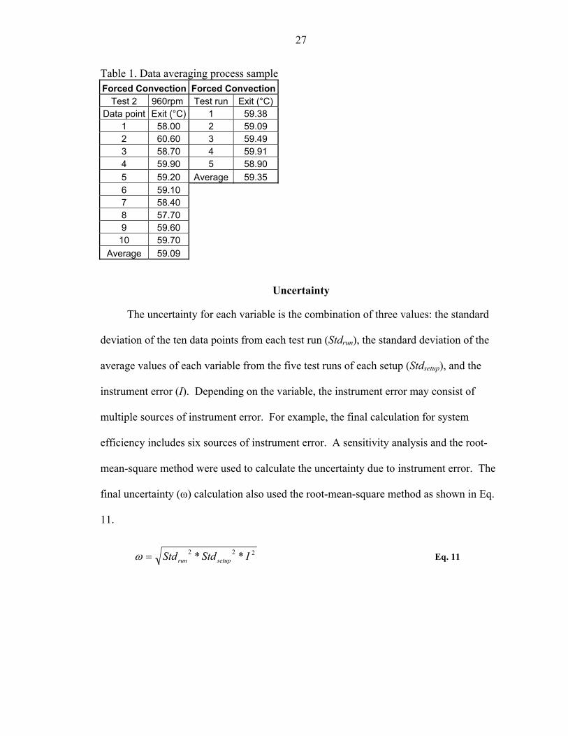
26 ∆Texit-in vs. Motor Speed...........................................................................................31
27 Mass flow rate vs. motor speed................................................................................32
28 Pressure ratio vs. motor speed..................................................................................33
29 Pressure ratio vs. mass flow rate ..............................................................................33
30 MC vs. motor speed .................................................................................................35
31 P η=100%vs. motor speed ............................................................................................35
32 MC vs. mass flow rate..............................................................................................36
33 P η=100%vs. mass flow rate.........................................................................................36
34 MC vs. P η=100%.........................................................................................................37
35 ηsys vs. motor speed ..................................................................................................39
36 ηsys vs. mass flow rate...............................................................................................40
37 ηA vs. motor speed....................................................................................................42
38 ηA vs. mass flow rate ................................................................................................43
39 ηsp vs. motor speed ...................................................................................................46
40 ηsp vs. mass flow rate................................................................................................46
41 Model predicted temperature profile for stock configuration at 900 rpm................53
42 Model predicted temperature profile for forced convection configuration at 1080 rpm ..................................................................................................................53
43 Model predicted Qdotremoved, total vs. motor speeds ...................................................57
44 Model predicted Qdotremoved, total vs. mass flow rates................................................58
45 Model predicted Motorlosses vs. motor speed ............................................................59
xi
46 Model predicted MElosses vs. motor speed ................................................................59
47 Model predicted Motorlosses vs. mass flow rate ........................................................60
48 Model predicted MElosses vs. mass flow rate ............................................................60
xii
Abstract of Thesis Presented to the Graduate School
of the University of Florida in Partial Fulfillment of the Requirements for the Degree of Master of Science
INVESTIGATION OF THE EFFECTS OF HEAT TRANSFER FROM A SCROLL COMPRESSOR THROUGH THE USE OF HEAT PIPES
By
Khiem Bao Dinh
August 2005
Chair: Vernon P. Roan Major Department: Mechanical and Aerospace Engineering
A scroll compressor is an efficient compressor design commonly used in air
conditioning and refrigeration applications. A relatively new application for compressors
is with fuel cell system pressurization in which they are used to increase the fuel cell
stack power output. The scroll compressor is one type of compressor being investigated
and integrated for use with these systems.
First developed by NASA, heat pipes are passive heat transfer devices with high
effective thermal conductivities and are now used in a wide range of common
applications that require the transfer of heat from one location to another. For example,
heat pipes are used in laptop computers to transfer heat from the microprocessor chip to a
fin assembly that is located more conveniently for packaging.
The purpose of this investigation was to provide information regarding the effect of
heat transfer from a scroll compressor by means of a heat pipe. A scroll compressor was
experimentally tested in three configurations: stock, integrated with a heat pipe rejecting
xiii
heat by free convection to the ambient atmosphere, and integrated with a heat pipe
rejecting heat by forced convection to the ambient atmosphere. Each configuration was
tested over a range of motor speeds. Furthermore, a simple computer model was
developed and used to further analyze the experimental data.
The results show that heat transfer from the scroll compressor through the use of
heat pipes has positive effects on increasing mass flow rates, reducing power
consumption and increasing efficiencies the compressor achieves. The information
presented in this thesis should be coupled with a cost and system integration analysis to
determine whether the use of heat pipes with scroll compressors would be beneficial.
1
CHAPTER 1 INTRODUCTION
Compressors are important to meeting the standard of living enjoyed by modern
society. The widespread use of vapor-compression refrigeration and air conditioning
around the world has made the compressor an indispensable device. The number of air
conditioning and refrigeration currently used numbers in the hundreds of millions, and
with the increasing development of third world countries even greater numbers of
compressors are being used.
A growing and potentially vast market for compressors lies with the increase of
fuel cells, a market projected to expand rapidly in the next few decades. Fuel cells are
viewed by many as the future of power generation as an alternative to fossil fuel
combustion and nuclear power generation. Two essential characteristics of fuel cells are
their high efficiency and environmental cleanliness, with their only emission being water.
The integration of compressors into fuel cell systems is being scrutinized since the
pressurization fuel cells provide a number of benefits.
The pressurization of a fuel cell through the use of a compressor causes the fuel cell
stack to have a higher efficiency and greater power density (desirable especially in
transportation applications). Furthermore, when a compressor is used in conjunction with
a Proton Exchange Membrane (PEM) fuel cell, the pressurization of the fuel cell aids in
the water management that is vital to the operation of a PEM fuel cell.3 The major
drawback of compressor use with fuel cells is the large power requirement for
compressor operation; the power drawn by the compressor may negatively impact the
2
overall fuel cell system more than the compressor aids the system. Therefore,
maximizing the efficiency of a compressor is critical in a fuel cell system.
In the simplest of terms, a compressor is a device used to increase the pressure of a
gas. For the compression of air, there are two general types of compressors: positive-
displacement and dynamic. Positive displacement compressors such as reciprocating and
rotary compressors increase the pressure of the air by decreasing its volume. Dynamic
air compressors use high velocity impellers to transfer angular momentum from the
impeller to the air thereby increasing the pressure of the air. Dynamic compressors
include axial flow and centrifugal compressors. In general, positive displacement
compressors are used for applications involving lower capacities (flow rates) and higher
pressure ratios whereas dynamic compressors are used for applications involving higher
capacities and lower pressure ratios.1
One desirable compression process would be an isothermal process where heat is
constantly removed during the compression process maintaining the gas at a constant
temperature. Isothermal compression reduces the work required to compress the gas
compared to compression processes where the gas temperature increases during
compression. This can be seen by the reduction of area under the pressure-volume curve
of isothermal compression versus polytropic compression in Figure 1. Very few real
compression processes are able to achieve isothermal compression, but multi-staged
compression processes have been devised where heat is removed between compression
stages to reduce compressor work.
A two-stage compression process with an intercooling intermediate step is also
shown in Figure 1. Intercooling is the removal of heat from a gas after being
3
compressed. In a staged compression system, the gas passes through one compressor
reaching a higher pressure, flows through a heat exchanger (intercooler) that cools the gas
to a lower temperature before passing through another compressor to reach a final
elevated pressure. The removal of heat in an intermediate step reduces the total
compressor work required versus compressing the fluid in one single step to the same
pressure without intercooling.5
Figure 1. Reduced compressor work due to cooling between stages
A compressor design commonly used in modern air conditioning units is the scroll
compressor. This compressor has a large, stationary surface area in contact with the
compressed gas during compression making it well suited to intercooling. The unique
geometry and operation of the scroll compressor allows for heat transfer during the
continuous compression process and internal to the compressor. Therefore, the heat
transfer during compression may allow for isothermal compression.
The intent of this study is to provide information on the effects of heat transfer
from a scroll compressor by means of an integrated heat pipe. It was hypothesized that
the main effect would be reduced power consumption for a given mass flow rate and
pressure ratio. A scroll compressor was tested over a variety of motor speeds in three
4
different configurations with each configuration having a different rate of heat transfer
from the compressor system. A computer model was also developed to better analyze the
experimental data in determining the performance of the compressor system.
5
CHAPTER 2 REVIEW OF LITERATURE
Scroll Compressor
In 1905, Leon Creux invented the scroll compressor, which is essentially a positive
displacement type compressor. The basis of the scroll compressor is two identical
involute spirals, or scrolls, that are nested together. With the two scrolls mated together,
they create a series of crescent shaped air pockets between them.4
The scroll compressor operates by keeping one scroll stationary (fixed scroll) while
the other scroll (orbiting scroll) orbits around the fixed scroll. The compression process
is shown in Figure 2. The first step is the intake of the air through the air inlets. The
second step is the sealing off of the air forming an air pocket. The orbiting scroll motion
causes the gas pockets to move towards the center of the scrolls while being reduced in
volume, hence the compression. Once the gas pocket reaches the center of the scrolls, the
tip of the orbiting scroll uncovers the discharge port located in the center of the fixed
scroll thereby beginning the discharge process. Due to the geometry of the scrolls, a
discharge valve is unnecessary as compared to a reciprocating type positive displacement
compressor. The discharge of air is nearly continuous as multiple pockets of gas are
compressed simultaneously (Figure 2, step 5).7
6
Figure 2. Compression process of a scroll compressor
Heat Pipe Background
Heat pipes are passive heat transfer devices with high effective thermal
conductivities that are based on a closed two-phase cycle and use the latent heat of
vaporization to transfer heat. The two-phase cycle allows heat pipes to have a heat
transfer capacity greater than the best solid conductors by several orders of magnitude
and leads the heat pipe to being a nearly isothermal device. In comparing aluminum and
copper rods with a heat pipe (all of 0.5m length and 1.27cm diameter) transmitting
twenty watts of power, the aluminum has a ∆T of 460 °C, the copper a ∆T of 206 °C, and
the heat pipe a ∆T of 6 °C.
Heat pipes typically consist of a sealed container with an internal wicking material
and working fluid (Figure 3) and can be broken down into three major sections:
evaporator, condenser, and an adiabatic/isothermal section in between. Heat addition
occurs at the evaporator where the working fluid in liquid phase is heated until it
7
vaporizes. The vapor then flows to the condenser and changes phase back to a liquid
releasing the latent heat of vaporization. Capillary forces in the wicking structure pump
the liquid back to the evaporator section.8
Figure 3. Heat pipe schematic
Changes in the heat flux into and out of the heat pipe results in a varied rate of
vaporization and condensation of the working fluid without significantly increasing the
operating temperature. Therefore, a heat pipe will operate at a relatively constant source
temperature over a wide range of power input by adjusting the rate at which the fluid
cycles through the heat pipe.
Next, the evaporator and condenser sections may be of different sizes and locations,
only needing common liquid and vapor streams. Therefore, high heat fluxes generated
over a small area (small evaporator section) can be dissipated over a larger area (large
condenser section) at a smaller heat flux. An additional advantage is the thermal
response time of a heat pipe; it’s faster than solid conductors and is also not a significant
function of length.6
8
CHAPTER 3 EXPERIMENTAL COMPONENTS AND SETUP
Stock Compressor Setup
The main component of the experimental test setup was the scroll compressor. A
prototype scroll compressor system sourced from Air Squared, Inc. consisted of: a three-
phase brushless DC motor, a compressor housing, and a compressor assembly (Figure
4)1.
Figure 4. Compressor system
The compressor housing attached to the motor acting as the mating adaptor for the
compressor assembly to the motor. The compressor assembly was composed of the fixed
and orbiting scrolls (Figure 5). A counterweighted shaft connected to the motor spins the
orbiting scroll (Figure 6).
1 Please see Appendix A for detailed compressor specifications
9
Figure 5. Compressor assembly
A high efficiency brushless DC motor was utilized in Air Squared’s system. The
compressor housing was vented to allow for airflow over the finned orbiting scroll for
heat rejection.
Figure 6. Compressor housing and counterweighted motor shaft
The orbiting scroll was mated to the fixed scroll by means of three shafts that are
located by ball bearings in each scroll for reduced friction. This scroll compressor
required no lubrication and utilized tip seals between the mating surfaces (scroll wall and
endplates) of the fixed and orbiting scrolls (Figure 7).
10
Figure 7. Fixed scroll
A ball bearing was used to mate the motor shaft to the orbiting scroll for reduced
friction (Figure 8) and two air inlet ports were used instead of one to reduce pumping
losses. These features all contributed to minimizing losses.
Figure 8. Orbiting scroll and scroll/motor shaft bearing
11
An adjustable, 30-volt and 5-amp power supply was used to power the motor
controller that in turn was used to power the motor.
The measurements of interest were: volumetric airflow rate, ambient air pressure,
compressor discharge air pressure, voltage and current input to the motor controller,
motor speed, and various temperatures. Airflow rate was measured using a digital
volumetric flow meter. Air pressure generated by the compressor was measured with a
liquid filled mechanical gauge and an indoor weather station measured ambient air
pressure. Digital multi-meters measured voltage, current, and motor speed.
Temperatures of interest were: air compressor intake and discharge, fixed scroll wall and
fin, motor, and motor controller. Temperatures were measured and data-logged using
Omega thermocouples and Iotech data acquisition hardware and software.
Air compressor intake and discharge temperatures were measured using
thermocouples placed in fittings attached to the air filter and compressor exit port
(Figures 9 and 10).
Figure 9. Air filter and intake temperature thermocouple
12
Figure 10. ¼ NPT-to-hose barb fitting with thermocouple
The fixed scroll was modified to allow for measurement of the scroll wall
temperatures. Three holes were drilled into the scroll wall at locations reflecting the
beginning, middle, and end (thermocouples Scroll 1, 2, and 3 respectively) of the airflow
path through the compressor (Figures 11 and 12). The thermocouples were inserted
approximately 20mm into the hole from the endplate side, which positioned the
thermocouples roughly in the middle of the scroll wall by height, and sealed with RTV
grey gasket maker.
Figure 11. Thermocouple holes in fixed scroll wall
13
Figure 12. Fixed scroll inlet ports, exit port, fins and thermocouples
Thermocouples were attached to a fin on the fixed scroll (Figure 13), the motor casing
(Figure 14), and motor controller (Figure 15) with adhesive backed thermocouples from
Omega.
Figure 13. Thermocouple on fixed scroll fin
14
Figure 14. Thermocouple on motor
Figure 15. Thermocouple on motor controller
The airflow path began through the air filter. A thermocouple was placed in a
fitting attached to the filter to measure air intake temperatures (Figures 9 and 10). Next,
the air flowed through a 10 cm length of 9.5 mm I.D clear vinyl tubing to the volumetric
flow meter before flowing through 50 cm of tubing to a T-fitting. From the T-fitting, the
airflow split to two 25 cm sections of tubing that attach to the two intake ports of the
compressor. At the compressor exit port, a ¼ NPT-to-hose barb fitting with a
thermocouple was screwed into the port allowing discharge air temperature measurement.
30 cm of 50 psi (345 kPa) rated fuel line was used on the compressor exit side, acting as
the discharge reservoir, because the vinyl tubing used on the intake side expanded under
pressure and elevated temperatures. A ball valve attached to the end of the fuel line acted
as a flow restriction and controlled the exit area of the flow. A T-fitting was placed 5 cm
15
before the ball valve as a pressure tap for the pressure gauge to measure discharge
pressure. Figure 16 is a path diagram for the airflow.
Figure 16. Airflow path diagram
The power used by the compressor system was determined by measuring the
voltage and current going to the motor controller. The motor and motor controller were
together considered to be an integrated system. Motor speed was determined by
measuring the frequency from a motor Hall effect sensor referenced to the ground of the
motor controller.
Heat Pipe Integration
The compressor required modification to accommodate the addition of a heat pipe
to the fixed scroll whose geometry was limiting in the configurations available. The
obstacles to fitting the heat pipe were the three ball bearings, air inlet ports, and the air
exit port. The heat pipe would have to go around these objects, as they could not be
modified. Therefore, this left two narrow paths between the bearings and air inlet and
exit ports where the heat pipes could be placed. Unfortunately, this resulted in the
removal of the third fixed scroll thermocouple (#3) that was located nearest the discharge
port.
16
The heat pipe diameter was the next variable to be determined. The maximum
diameter heat pipe that could be fitted was 12.7 mm diameter. An alternative option was
the use of two 6.35 mm diameter heat pipes in place of a single 12.7 mm diameter pipe to
increase the contact surface area between the heat pipes and fixed scroll. It was
determined that the heat transfer properties of the 6.35 mm heat pipes were relatively
limited and therefore, the 12.7 mm heat pipe was chosen. The larger diameter pipe also
reduced the machining necessary, thus easing the modification.
The first step in machining the fixed scroll was using a 12.7 mm diameter end mill
creating the paths for the heat pipe through the fins. Next, a circular groove of 6.35 mm
radius was machined using a 12.7 mm diameter ball-end end mill, resulting in the mating
interface between the heat pipes and fixed scroll surface (Figure 17).
Figure 17. Grooves machined into fixed scroll between bearings and air inlet and exit ports
The fixed scroll end plate was 5 mm thick limiting the possible depth of the groove
resulting in a machined groove depth of 1.78 mm (Figure 18). This depth created a
17
mating interface area totaling approximately 19.5 cm2 (2 grooves x 9.74 mm arc length x
100 mm groove length) while not affecting the structural rigidity of the fixed scroll.
Figure 18. Depth of groove machined into fixed scroll
The heat pipe was fabricated with the assistance of Heat Pipe Technology, Inc. and
had the form of a U-shape with a length of 61 cm. A 30.5 cm section of the condenser
side of the heat pipe was finned using aluminum fins of 25 mm width, 63.5 mm length,
and 4.33 fins per centimeter. Three thermocouples were attached to the heat pipe: one on
each side of the U (labeled Pipe 1,2) and one in the fin assembly (Pipe 3). Figures 19 and
20 show the heat pipe, fins, and thermocouples.
Figure 19. Heat pipe assembly
18
Figure 20. Thermocouple placed in heat pipe fins
The heat pipe fit tightly into the machined grooves but a small clamp fitting was
fabricated to secure the heat pipe to the endplate (Figure 21). Thermal conducting paste
was used at the interface between the heat pipe and the endplate to ensure good heat
conduction (Figure 22).
Figure 21. Heat pipe clamped to fixed scroll
19
Figure 22. Interface of heat pipe and fixed scroll
The forced convection tests required the addition of fans to the heat pipe assembly
to reject heat to the atmosphere. Four small fans generally used for cooling CPU chips in
computers were attached to the heat pipe assembly and powered by an additional power
supply. To ensure airflow through the fins, two metal plates were attached to the sides of
the fins to duct the airflow. Figures 23 and 24 show the fans and metal plates attached to
the fins of the heat pipe.
Figure 23. Fans mounted to the heat pipe assembly
21
CHAPTER 4 EXPERIMENTAL TEST PROCEDURE AND DATA ANALYSIS
System Characterization Tests
A series of initial system characterization tests were performed to determine the
range of the measured parameters of power input, volumetric flow rates, pressure ratios
and thermocouple temperatures. The test plan required steady state conditions; therefore,
these initial tests were performed to determine the time required for the system to reach
steady state with respect to scroll and discharge air temperatures. Figure 25 shows an
initial test run and the time required for the temperatures to reach a steady state (up to 2
hours), defined as the mean temperature of each thermocouple reading varying by less
than 1 °C over a ten-minute time interval.
Thermocouple Measurements
0102030405060708090
100
0 1000 2000 3000 4000 5000 6000 7000 8000
time (sec)
tem
pera
ture
(°C
)
intake scroll 1 scroll 2 scroll 3 exit fin motor controller
Figure 25. Initial test temperature graph
22
The initial tests exposed other characteristics of importance. Scroll 1, Scroll 2, and
Scroll 3 represent the three thermocouples placed into the fixed scroll wall (Figure 12).
Figure 25 shows Scroll 1 maintained the lowest temperature, Scroll 2 an intermediate
temperature, and Scroll 3 the highest temperature. It was hypothesized these
temperatures reflected the increasing air temperature as it was compressed along the
airflow path. Also, the discharge air temperature was directly related to the fixed scroll
wall temperature shown by the discharge air temperature increasing proportionally to the
fixed scroll wall temperatures.
Additional temperatures of importance were the fixed scroll fin, motor, and motor
controller. The fixed scroll fin and motor temperatures were also directly related to the
fixed scroll wall temperatures. The motor controller temperature was found to increase
similarly to the motor during an initial test and therefore, a fan was placed over the motor
controller to maintain a cool temperature.
Final observations from the initial tests relate to the volumetric airflow rate, motor
controller power input, discharge air pressure, and motor speed. The first three variables
were somewhat unsteady, given a steady motor speed. The motor speed fluctuated over a
range of 1.5 rpm at motor speeds of 960 rpm and 1020 rpm, less than 0.14% of full scale
(1080 rpm). Motor speed fluctuated over a range of 0.3 rpm at 900 rpm and 0.6 rpm
1080 rpm. The measured discharge air pressure oscillated apparently due to the nature of
the scroll compressor. Though the air pressure gauge was liquid filled, the reading
oscillated approximately 0.25 psi (1.7 kPa) over the range of 15-20 psig (103-138 kPa).
The current input to the motor controller varied up to 0.15 amps (over a range of 3-5
amps) given a constant voltage input at constant motor speed. Increased current at
23
constant motor speed resulted in increased air volumetric flow rate and discharge
pressure. Based on these system characteristics, motor speed and airflow exit orifice area
could be assumed to be constant during the test runs and the other measured variables
would be continuously monitored.
Experimental Test Procedure
A fixed ball valve position at the airflow exit, and four motor speeds (900 rpm, 960
rpm, 1020 rpm, and 1080 rpm) were used for all test runs. For each test run, the motor
was started and run at 900 rpm until the thermocouple temperatures reached steady state.
Data was then recorded once every minute until ten data points were collected. Next, the
motor speed was increased to 960 rpm and temperatures allowed to reach steady state
before recording another set of data points. This procedure was repeated for 1020 rpm
and 1080 rpm. The values recorded were: temperature readings (air intake and discharge,
Scroll 1-2, Pipe 1-3, fin, motor, motor controller), voltage and current to the motor
controller, volumetric air flow rate, ambient air pressure, and discharge air gauge
pressure from the compressor. These values were then used to calculate a number of
parameters. It is important to note that the parameters calculated using the measured
discharge air temperature do not represent truly accurate values because the measured
temperatures were dependent on thermocouple location; however, the parameters may
confidently be compared relative to each other as they all used data from the same
thermocouple and location.
Inlet air density from the equation of state for an ideal gas:
in
amb
TRPM
**
=ρ Eq. 1
M = molecular weight of air
24
Pamb = ambient air pressure
R = universial gas constant
inT = compressor intake temperature
Mass flow rate:
ρ*Vm && = Eq. 2
V& = volumetric flow rate
Pressure ratio:
ambpdpPR = Eq. 3
dp = discharge pressure = Pdischarge,gage + Pamb,abs
Net rate of heat addition:
)(***Q inexitPnet TTCmhm −≈∆= &&& Eq. 4
exitT = compressor discharge air temperature
h∆ = change of enthalpy
PC = average specific heat
netQ& represents the net power (approximated by the rate of heat addition) added to the air
flowing through the compressor. netQ& also approximates the change of enthalpy.
Power for 100% efficient isentropic compressor:
⎟⎟⎠
⎞⎜⎜⎝
⎛−=
−
= 1***1
%100k
k
inP PRTCmP &η Eq. 5
Pη=100% is an approximated power requirement of an isentropic compression process
based on the measured air temperatures, volumetric flow rates, and pressures. This value
25
provides a basis for comparison of the relative work performed by each compressor
configuration. By using this value, it is assumed the desired compressor work is only to
increase the pressure ratio of the air and that the temperature of the discharge air is
irrelevant.
Motor controller input power:
MC = AV * Eq. 6
V = measured voltage input to the motor controller
A = measured current input to the motor controller
Effective system efficiency:
ηsys = MC
P %100=η Eq. 7
For this experimental setup, ηsys is the best indicator of the effectiveness of the integration
of a heat pipe in increasing the overall performance of this scroll compressor system.
Availabilty analysis:
( )PRRTT
cSin
exitp lnln −⎟⎟
⎠
⎞⎜⎜⎝
⎛=∆ Eq. 8
( )( )SThhmA ininexit ∆−−=∆ *& Eq. 9
hexit = enthalpy at Texit
hin = enthalpy at Tin
The availbilty between the inlet and exit states of the compressor was calculated for each
case using Eq. 8 and Eq. 9. The values for enthalpy were obtained from tables.5
Availability-based efficiency:
26
MC
AA
∆=η Eq. 10
The availability-based efficiency, ηA, compares the minimum power required to go from
the inlet state to the exit state (isothermal compression followed by isentropic heat
addition) and the motor controller input power. This is relevant if the discharge
temperature of the air is important and a higher discharge air temperature is desireable.2, 5
Five test runs were completed for each compressor setup: stock compressor,
compressor with heat pipes and free convection (heat rejection to the atmosphere by free
convection from the heat pipe, Figure 20), and with heat pipes and forced convection
(heat rejection to the atmosphere by forced convection, Figure 23). For each test run, the
ten data points recorded for each variable at each motor speed were averaged to obtain a
single value representing that motor speed and test run. For example, on test run #2 for
the forced convection heat pipe setup, the ten data points for discharge air temperature
taken at a motor speed of 960 rpm were averaged together to obtain a single value of
59.09 °C. Next, this value was averaged with the average discharge air temperature
values at 960 rpm from the other 4 test runs to obtain a value of 59.35 °C. This final
value is taken to be the standard value for discharge air temperature at a motor speed of
960 rpm for the forced convection heat pipe setup (Table 1). Standard deviations were
also calculated for all variables (Appendix B).
27
Table 1. Data averaging process sample Forced Convection Forced Convection
Test 2 960rpm Test run Exit (°C)Data point Exit (°C) 1 59.38
1 58.00 2 59.09 2 60.60 3 59.49 3 58.70 4 59.91 4 59.90 5 58.90 5 59.20 Average 59.35 6 59.10 7 58.40 8 57.70 9 59.60 10 59.70
Average 59.09
Uncertainty
The uncertainty for each variable is the combination of three values: the standard
deviation of the ten data points from each test run (Stdrun), the standard deviation of the
average values of each variable from the five test runs of each setup (Stdsetup), and the
instrument error (I). Depending on the variable, the instrument error may consist of
multiple sources of instrument error. For example, the final calculation for system
efficiency includes six sources of instrument error. A sensitivity analysis and the root-
mean-square method were used to calculate the uncertainty due to instrument error. The
final uncertainty (ω) calculation also used the root-mean-square method as shown in Eq.
11.
222 ** IStdStd setuprun=ω Eq. 11
28
Experimental Data and Analysis
Motor Speeds
The tests were conducted with motor speeds as close as possible to the ideal speeds
of 900 rpm, 960 rpm, 1020 rpm, and 1080 rpm. Average actual test speeds are listed in
Table 2.
Table 2. Actual test speeds STOCK
rpm 900.32 960.48 1020.76 1080.78
FREE CONVECTION
rpm 900.27 960.38 1020.21 1079.99
FORCED CONVECTION
rpm 900.41 960.41 1020.28 1080.52
Compressor Component Temperatures
The first parameters of interest are the temperatures of the compressor components:
Scroll 1-2, Fin, Motor, and Pipe 1-3. Table 3 shows the average values from the tests.
The addition of the heat pipe in free convection and forced convection configurations
reduced the temperatures of the fixed scroll wall, fin, and motor. The compressor in the
stock configuration showed a slight temperature gradient between Scroll 1 and Scroll 2;
the cause was hypothesized to be the increasing air temperature as it was compressed and
29
moved along the flow path. The heat pipe in free convection configuration had the effect
of relatively equalizing the scroll wall temperatures at the thermocouple locations while
the forced convection configuration reversed the stock temperature gradient.
Also of importance was the reduction in operating temperature of the motor. Heat
conducted from the motor to the fixed scroll by way of the compressor housing reducing
the motor operating temperature and potentially increasing the motor efficiency and
longevity.
Table 3. Compressor component temperatures STOCK - Temperatures in °C
rpm Scroll 1 Scroll 2 Fin Motor 900 58.30 60.26 53.36 51.46 960 63.06 64.65 56.75 54.97
1020 66.04 68.17 59.65 57.34 1080 70.08 72.66 63.50 61.37
FREE CONVECTION - Temperatures in °C
rpm Scroll 1 Scroll 2 Fin Motor Pipe 1 Pipe 2 Pipe 3 900 51.44 52.03 46.62 47.36 44.63 44.08 42.55 960 53.72 54.02 48.12 49.63 46.43 46.08 44.32
1020 58.22 58.69 52.34 53.57 50.18 49.75 48.05 1080 61.67 61.92 55.09 56.36 52.62 52.11 50.17
FORCED CONVECTION - Temperatures in °C
rpm Scroll 1 Scroll 2 Fin Motor Pipe 1 Pipe 2 Pipe 3 900 40.30 39.00 36.17 40.41 28.84 28.86 27.35 960 41.16 40.05 36.92 42.38 28.34 28.39 26.26
1020 44.51 42.39 39.30 45.07 30.06 30.02 28.59 1080 46.30 43.81 40.44 46.57 29.95 29.74 27.86
The heat pipe in free convection configuration was cooler than the scroll wall and
fin and exhibited increased temperatures with increased motor speed. The temperature of
the heat pipe in the forced convection configuration was also cooler than the scroll wall
and fin. The difference between the heat pipe and scroll wall temperatures was greater in
the forced convection configuration compared to the difference in the free convection
30
configuration, which was due to a greater heat flux. The heat pipe in forced convection
also demonstrated a relatively constant temperature over the range of motor speeds
demonstrating the heat pipe’s ability to transfer varying rates of heat while maintaining a
near constant temperature. In this case, the heat transfer rate by forced convection on the
condenser side (fins) of the heat pipe was nearly able to match the increased heat flux
from the evaporator side (fixed scroll). Also, the heat pipe operated nearly isothermally
as expected; thermocouples Pipe 1 and 2 that were placed on the tubes were nearly
identical in all cases and Pipe 3 in the fin being slightly cooler.
Air Discharge Temperature and ∆Texit-in
The addition of the heat pipe reduced the discharge air temperature up to 25 °C
compared to the stock configuration. The intake air temperature, exit (discharge) air
temperature, and their difference, ∆Texit-in, are listed in Table 4.
Table 4. Air intake and discharge temperatures and ∆Texit-in STOCK - Temperatures in °C
rpm Tin Texit ∆Texit-in 900 24.99 75.67 50.69 960 24.67 82.10 57.43
1020 24.70 87.20 62.50 1080 24.64 93.56 68.93
FREE CONVECTION - Temperatures in °C
rpm Tin Texit ∆Texit-in 900 24.68 67.17 42.48 960 24.73 72.19 47.46
1020 25.39 78.02 52.62 1080 25.20 83.96 58.76
FORCED CONVECTION - Temperatures in °C
rpm Tin Texit ∆Texit-in 900 25.09 55.73 30.64 960 24.72 59.35 34.64
1020 25.38 64.35 38.97 1080 24.73 68.05 43.31
31
Figure 26 shows the reduced ∆Texit-in of the heat pipe configurations compared to
stock with the forced convection configuration demonstrating the lowest ∆Texit-in for all
motor speeds.
∆Texit-in vs. Motor Speed
forced = 0.0706x - 33.014R2 = 0.9996
free = 0.0901x - 38.895R2 = 0.9974
stock = 0.0994x - 38.548R2 = 0.9972
20.00
30.00
40.00
50.00
60.00
70.00
80.00
870 900 930 960 990 1020 1050 1080
motor speed (rpm)
∆T e
xit-i
n (°
C)
stock free forced
Figure 26. ∆Texit-in vs. motor speed.
Mass Flow Rate and Pressure Ratio
The reduced air temperatures due to the reduced temperatures of the fixed scroll
wall directly increased the mass flow rate of air for a given motor speed.
Correspondingly, the pressure ratios achieved by the compressor also increased. Table 5
lists the mass flow rates and the pressure ratios for each case. Figures 27-29 compare the
motor speeds, mass flow rates, and pressure ratios.
The free convection and forced convection heat pipe configurations had increased
mass flow rates and pressure ratios as compared to the stock compressor. The stock and
free convection configurations had nearly identical pressure ratios based on mass flow
32
rates while the forced convection setup exhibited slightly lower pressure ratios for the
same mass flow rates.
Table 5. Mass flow rates and pressure ratios STOCK
rpm m& (kg/hr) PR 900 2.18 2.00 960 2.28 2.07 1020 2.38 2.17 1080 2.49 2.25
FREE CONVECTION
rpm m& (kg/hr) PR 900 2.22 2.02 960 2.33 2.12 1020 2.42 2.20 1080 2.53 2.29
FORCED CONVECTION
rpm m& (kg/hr) PR 900 2.26 2.03 960 2.39 2.15 1020 2.49 2.24 1080 2.62 2.36
Mass Flow Rate vs. Motor Speed
forced = 0.002x + 0.4765R2 = 0.9986
free = 0.0017x + 0.669R2 = 0.9985
stock = 0.0017x + 0.6271R2 = 1
2.10
2.20
2.30
2.40
2.50
2.60
2.70
870 900 930 960 990 1020 1050 1080
motor speed (rpm)
mas
s flo
w ra
te (k
g/hr
)
stock free forced
Figure 27. Mass flow rate vs. motor speed
33
Pressure Ratio vs. Motor Speed
forced = 0.0018x + 0.4315R2 = 0.997
free = 0.0015x + 0.6926R2 = 0.9982
stock = 0.0015x + 0.6808R2 = 0.9937
1.95
2.00
2.05
2.10
2.15
2.20
2.25
2.30
2.35
2.40
870 900 930 960 990 1020 1050 1080
motor speed (rpm)
pres
sure
ratio
stock free forced
Figure 28. Pressure ratio vs. motor speed
Pressure Ratio vs. Mass Flow Rate
stock = 0.8456x + 0.1508R2 = 0.9933
free = 0.8564x + 0.1204R2 = 0.9986
forced = 0.8979x + 0.0027R2 = 0.9993
1.95
2.00
2.05
2.10
2.15
2.20
2.25
2.30
2.35
2.40
2.10 2.20 2.30 2.40 2.50 2.60 2.70
mass flow rate (kg/hr)
pres
sure
ratio
stock free forced
Figure 29. Pressure ratio vs. mass flow rate
34
Power Consumption
Table 6 lists the calculated values for MC, netQ& , and Pη=100%.
Table 6. Calculated power values STOCK - Power in watts
rpm MC netQ& P η =100%
900 93.01 30.78 39.66 960 106.13 36.54 43.77 1020 120.71 41.57 49.32 1080 135.24 47.83 54.11
FREE CONVECTION - Power in watts
rpm MC netQ& P η =100%
900 95.37 26.29 41.03 960 109.69 30.88 46.42 1020 124.31 35.58 51.17 1080 140.16 41.50 56.23
FORCED CONVECTION - Power in watts
rpm MC netQ& P η =100%
900 98.38 19.33 42.32 960 113.31 23.07 48.64 1020 128.90 27.10 53.93 1080 145.49 31.70 60.63
MC increased for a given motor speed (Figure 30) with the heat pipe installed
because the mass flow rates and pressure ratios were increased. Therefore, to maintain
the same motor speed, more power was required to flow the additional air and compress
the air to an increased pressure ratio. The increased mass flow rates and pressure ratios
also translated into more relative compressor power as shown by the increased values of
Pη=100% (Figure 31). MC and Pη=100% were also compared on a mass flow rate basis
(Figures 32 and 33). This is most applicable to the cases of the stock configuration and
the free convection configuration as they exhibited nearly identical pressure ratios versus
mass flow rates (Figure 29). On a mass flow rate basis, the heat pipe configurations had
35
lower values of MC indicating reduced power consumption. The trends for Pη=100%
matched those of the pressure ratio trends on a mass flow rate basis. Therefore, the heat
pipe configurations were doing the same relative compressor work with reduced power
consumption (Figure 34).
MC vs. Motor Speed
forced = 0.2615x - 137.45R2 = 0.9995
free = 0.2487x - 128.91R2 = 0.9994
stock = 0.2348x - 118.85R2 = 0.9994
90.00
100.00
110.00
120.00
130.00
140.00
150.00
870 900 930 960 990 1020 1050 1080
motor speed (rpm)
MC
(wat
ts)
stock free forced
Figure 30. MC vs. motor speed
P η=100% vs. Motor Speed
forced = 0.1003x - 47.952R2 = 0.9983
free = 0.0841x - 34.527R2 = 0.9995
stock = 0.0813x - 33.779R2 = 0.997
35.00
40.00
45.00
50.00
55.00
60.00
65.00
870 900 930 960 990 1020 1050 1080
motor speed (rpm)
P η=
100%
(wat
ts)
stock free forced
Figure 31. P η=100%vs. motor speed
36
MC vs. Mass Flow Rate
forced = 131.62x - 199.88R2 = 0.9986
free = 143.97x - 224.83R2 = 0.9978
stock = 136.36x - 204.34R2 = 0.9993
90.00
100.00
110.00
120.00
130.00
140.00
150.00
2.10 2.20 2.30 2.40 2.50 2.60 2.70
mass flow rate (kg/hr)
MC
(wat
ts)
stock free forced
Figure 32. MC vs. mass flow rate
P η=100% vs. Mass Flow Rate
forced = 50.55x - 72.057R2 = 1
free = 48.699x - 67.049R2 = 0.9996
stock = 47.179x - 63.353R2 = 0.9968
35.00
40.00
45.00
50.00
55.00
60.00
65.00
2.10 2.20 2.30 2.40 2.50 2.60 2.70
mass flow rate (kg/hr)
P η
=100
% (w
atts
)
stock free forced
Figure 33. P η=100%vs. mass flow rate
37
MC vs. P η=100%
forced = 2.6034x - 12.251R2 = 0.9984
free = 2.9566x - 26.638R2 = 0.9984
stock = 2.8848x - 20.987R2 = 0.9988
90.00
100.00
110.00
120.00
130.00
140.00
150.00
35.00 40.00 45.00 50.00 55.00 60.00 65.00
P η=100% (watts)
MC
(wat
ts)
stock free forced
Figure 34. MC vs. P η=100%
Using the equations from the linear trendlines established in Figure 34, MC was
calculated for each of the configurations over the range of Pη=100% tested (Table 7). The
data for the free and forced convection configurations were extrapolated down to a
Pη=100% of 38 watts even though there were not tested down to that level. Likewise, the
stock and free convection configurations were extrapolated up to a Pη=100% of 62 watts.
The free convection configuration required a MC of ~96.7% relative to the stock
configuration at a Pη=100% of 38 watts; thus, MC was reduced ~3.3%. At a Pη=100% of 62
watts, the free convection configuration showed a reduction of ~0.9% in MC relative to
stock. The forced convection configuration showed a reduction of MC of ~2.2% at a
Pη=100% of 38 watts and a larger reduction of ~5.5% at a Pη=100% of 62 watts. It is
expected the forced convection configuration will further reduce MC relative to the stock
configuration at higher compressor loads.
38
Table 7. Calculated MC from trendlines for tested range of Pη=100% MC - Units in watts Relative to stock
Pη =100% Stock Free Forced Freerelative (%) Forcedrelative (%) 38 88.6 85.7 86.7 96.7 97.8 40 94.4 91.6 91.9 97.1 97.3 42 100.2 97.5 97.1 97.4 96.9 44 105.9 103.5 102.3 97.6 96.6 46 111.7 109.4 107.5 97.9 96.2 48 117.5 115.3 112.7 98.1 95.9 50 123.3 121.2 117.9 98.3 95.7 52 129.0 127.1 123.1 98.5 95.4 54 134.8 133.0 128.3 98.7 95.2 56 140.6 138.9 133.5 98.8 95.0 58 146.3 144.8 138.7 99.0 94.8 60 152.1 150.8 144.0 99.1 94.6 62 157.9 156.7 149.2 99.2 94.5
Effective System Efficiency
The calculated values for the effective system efficiency, ηsys, are listed in Table 8
and graphed in Figures 35 and 36. From the experimental data, the heat transfer provided
by the heat pipe increased the effective system efficiency. Comparing ηsys on a mass flow
rate basis may give a better indication as to the differences created by the heat transfer
but unfortunately, due to the relatively large uncertainty associated with the ηsys
calculation, there is no clear separation between the values from the stock and free
convection or free and forced convection configurations. However, the separations
between the values of the stock and forced convection configurations are mostly well
defined. On either a motor speed or mass flow rate basis, the forced convection
configuration exhibits a higher ηsys versus the stock setup. The values of ηsys for the free
convection configuration fall between the other two configurations.
39
Table 8. Effective system efficiencies, ηsys STOCK
rpm ηsys (%) 900 42.61 960 41.23
1020 40.84 1080 39.99
FREE CONVECTION
rpm ηsys (%) 900 43.00 960 42.30
1020 41.14 1080 40.10
FORCED CONVECTION
rpm ηsys (%) 900 42.97 960 42.90
1020 41.81 1080 41.65
ηsys vs. Motor Speed
forced = -0.0084x + 50.629R2 = 0.8701
free = -0.0164x + 57.91R2 = 0.9905
stock = -0.0137x + 54.756R2 = 0.9508
39.00
39.50
40.00
40.50
41.00
41.50
42.00
42.50
43.00
43.50
44.00
870 900 930 960 990 1020 1050 1080
motor speed (rpm)
η sys
(%)
stock free forced
Figure 35. ηsys vs. motor speed
40
ηsys vs. Mass Flow Rate
forced = -4.1595x + 52.489R2 = 0.8457
free = -9.4857x + 64.182R2 = 0.983
stock = -7.9696x + 59.761R2 = 0.9519
39.0039.5040.0040.5041.0041.5042.0042.5043.0043.5044.00
2.10 2.30 2.50 2.70
mass flow rate (kg/hr)
η sys
(%)
stock free forced
Figure 36. ηsys vs. mass flow rate
Using the equations from the linear trendlines established in Figures 35 and 36, ηsys
was calculated for each of the configurations over the range of motor speeds and mass
flow rates tested (Tables 9 and 10). When compared over the range of motor speeds
tested, the free convection configuration had a relative ηsys of ~101.7% compared to the
stock configuration at 900 rpm. Hence, the free convection configuration showed an
improvement of ~1.7%. This improvement decreased to ~0.6% at 1080 rpm. The forced
convection configuration showed an improvement of ~1.5% at 900 rpm which increased
to ~4.0% at 1080 rpm.
Table 9. Calculated ηsys from trendlines for tested range of motor speeds ηsys - Units in % Relative to stock rpm Stock Free Forced Freerelative Forcedrelative 900 42.4 43.2 43.1 101.7 101.5 930 42.0 42.7 42.8 101.5 101.9 960 41.6 42.2 42.6 101.4 102.3 990 41.2 41.7 42.3 101.2 102.7 1020 40.8 41.2 42.1 101.0 103.1 1050 40.4 40.7 41.8 100.8 103.6 1080 40.0 40.2 41.6 100.6 104.0
41
For comparison on a mass flow rate basis, the data for the free and forced
convection configurations was extrapolated down to a mass flow rate of 2.18 kg/hr.
Likewise, the stock and free convection configurations were extrapolated up to 2.62
kg/hr. From Table 10, the free convection configuration showed a relative increase of
~2.6% at 2.18 kg/hr flowrate which reduced to ~1.2% at 2.62 kg/hr flowrate. The forced
convection configuration showed an improvement of ~2.4% at 2.18 kg/hr flowrate which
increased to ~7.0% at 2.62 kg/hr flowrate.
Table 10. Calculated ηsys from trendlines for tested range of mass flow rates ηsys - Units in % Relative to stock
m& (kg/hr) Stock Free Forced Freerelative Forcedrelative 2.18 42.4 43.5 43.4 102.6 102.4 2.22 42.1 43.1 43.3 102.5 102.8 2.26 41.7 42.7 43.1 102.4 103.2 2.30 41.4 42.4 42.9 102.3 103.6 2.34 41.1 42.0 42.8 102.1 104.0 2.38 40.8 41.6 42.6 102.0 104.4 2.42 40.5 41.2 42.4 101.9 104.8 2.46 40.2 40.8 42.3 101.7 105.2 2.50 39.8 40.5 42.1 101.6 105.7 2.54 39.5 40.1 41.9 101.4 106.1 2.58 39.2 39.7 41.8 101.3 106.5 2.62 38.9 39.3 41.6 101.2 107.0
Availability-Based Efficiency
The calculated values for ηA are listed in Table 11 and graphed in Figures 37 and
38. The calculated ηA was lower for all motor speeds for the heat pipe configurations
compared to the stock configuration. This was also the general trend for the range of
mass flow rates covered by all three configurations. This was due to the lower discharge
temperatures of the air from the heat pipe configurations resulting in a lower change in
enthalpy.
42
Table 11. Calculated availabilty-based efficiency
STOCK rpm ∆A (watts) MC (watts) ηA (%) 900 38.24 93.01 41.11 960 42.36 106.13 39.92
1020 47.53 120.71 39.38 1080 52.71 135.24 38.98
FREE CONVECTION
rpm ∆A (watts) MC (watts) ηA (%) 900 38.59 95.37 40.46 960 43.69 109.69 39.83
1020 48.73 124.31 39.20 1080 53.67 140.16 38.29
FORCED CONVECTION
rpm ∆A (watts) MC (watts) ηA (%) 900 39.13 98.38 39.78 960 44.55 113.31 39.32
1020 49.84 128.90 38.67 1080 55.43 145.49 38.09
ηA vs. Motor Speed
forced = -0.0095x + 48.374R2 = 0.996
free = -0.0119x + 51.232R2 = 0.9906
stock = -0.0115x + 51.267R2 = 0.9345
37.00
37.50
38.00
38.50
39.00
39.50
40.00
40.50
41.00
41.50
42.00
870 900 930 960 990 1020 1050 1080
motor speed (rpm)
η A (%
)
stock free forced
Figure 37. ηA vs. motor speed
43
ηA vs. Mass Flow Rate
forced = -4.7746x + 50.624R2 = 0.9921
free = -6.8926x + 55.83R2 = 0.9898
stock = -6.6984x + 55.473R2 = 0.9354
37.00
37.50
38.00
38.50
39.00
39.50
40.00
40.50
41.00
41.50
42.00
2.10 2.20 2.30 2.40 2.50 2.60 2.70
mass flow rate (kg/hr)
η A (%
)
stock free forced
Figure 38. ηA vs. mass flow rate
Using the equations from the linear trendlines established in Figures 37 and 38, ηA
was calculated for each of the configurations over the range of motor speeds and mass
flow rates tested (Tables 12 and 13). The ηA for the free convection configuration
relative to stock was ~1.0% lower at a motor speed of 900 rpm and ~1.2% lower at a
motor speed of 1080 rpm. The ηA for the forced convection configuration relative to
stock was ~2.7% lower at 900 rpm but the difference reduced to ~1.9% at 1080 rpm.
Table 12. Calculated ηA from trendlines for tested range of motor speeds ηA - Units in % Relative to stock
rpm Stock Free Forced Freerelative Forcedrelative 900 40.9 40.5 39.8 99.0 97.3 930 40.6 40.2 39.5 99.0 97.5 960 40.2 39.8 39.3 99.0 97.6 990 39.9 39.5 39.0 98.9 97.7
1020 39.5 39.1 38.7 98.9 97.8 1050 39.2 38.7 38.4 98.8 98.0 1080 38.8 38.4 38.1 98.8 98.1
44
Comparision on a mass flow rate basis showed the free convection configuration
having a ηA ~0.2%-0.4% lower the than stock configuration over the extrapolated range.
The forced convection configuration had a ηA ~1.6% lower than stock at a 2.18 kg/hr
flow rate. However, it had a ηA ~0.5% higher when compared at a 2.62 kg/hr flow rate.
It is expected that the forced convection configuration will have an increased ηA relative
to stock at higher than tested flow rates.
Table 13. Calculated ηA from trendlines for tested range of mass flow rates ηA - Units in % Relative to stock
m& (kg/hr) Stock Free Forced Freerelative Forcedrelative 2.18 40.9 40.8 40.2 99.8 98.4 2.22 40.6 40.5 40.0 99.8 98.6 2.26 40.3 40.3 39.8 99.8 98.8 2.30 40.1 40.0 39.6 99.8 98.9 2.34 39.8 39.7 39.5 99.8 99.1 2.38 39.5 39.4 39.3 99.7 99.3 2.42 39.3 39.1 39.1 99.7 99.5 2.46 39.0 38.9 38.9 99.7 99.7 2.50 38.7 38.6 38.7 99.7 99.9 2.54 38.5 38.3 38.5 99.6 100.1 2.58 38.2 38.0 38.3 99.6 100.3 2.62 37.9 37.8 38.1 99.6 100.5
Approximated Compressor Efficiency
It was possible to approximate compressor efficiency, ηsp, comparing shaft power
to isentropic compression power (Pη =100%) from the experimental data using the
specifications of the compressor. The forced convection configuration at 1080 rpm had
the following average values: MC = 145.49 watts, volumetric flow rate = 36.01 LPM,
and Pdischarge,gage = 20.44 psi (141 kPa) (Appendix B). This closely matches the
specifications for the compressor at 1000 rpm of: volumetric flow rate = 36 LPM,
Pdischarge,gage = 20 psi (138 kPa), and shaft power = 109 watts (Appendix A). From this
information, the approximate percentage of power converted from MC to compressor
45
shaft power is 75%. Assuming this percentage remains constant for all cases, an
approximated shaft power for each case can be calculated from Eq. 12. This assumption
was deemed reasonable because of the limited range of motor speeds tested. ηsp was
calculated from Eq. 13. Table 14 lists the approximated shaft power, SPapprox, and ηsp for
each case. Figures 39 and 40 show the trends of ηsp are the same as ηsys.
Approximated shaft power:
75.0*MCSPapprox = Eq. 12
Approximated compressor efficiency:
approx
sp SPP 100== ηη Eq. 13
Table 14. Appoximated compressor shaft power and ηsp STOCK - Power in watts
rpm MC SPapprox. ηsp (%) 900 93.01 69.8 56.9 960 106.13 79.6 55.0 1020 120.71 90.5 54.5 1080 135.24 101.4 53.3
FREE CONVECTION - Power in watts
rpm MC SPapprox. ηsp (%) 900 95.37 71.5 57.4 960 109.69 82.3 56.4 1020 124.31 93.2 54.9 1080 140.16 105.1 53.5
FORCED CONVECTION - Power in watts
rpm MC SPapprox. ηsp (%) 900 98.38 73.8 57.4 960 113.31 85.0 57.2 1020 128.90 96.7 55.8 1080 145.49 109.1 55.6
46
ηsp vs. Motor Speed
52.00
53.00
54.00
55.00
56.00
57.00
58.00
59.00
870 900 930 960 990 1020 1050 1080
motor speed (rpm)
η sp(
%)
stock free forced
Figure 39. ηsp vs. motor speed
ηsp vs. Mass Flow Rate
52.00
53.00
54.00
55.00
56.00
57.00
58.00
59.00
2.10 2.20 2.30 2.40 2.50 2.60 2.70
mass flow rate (kg/hr)
η sp(
%)
stock free forced
Figure 40. ηsp vs. mass flow rate
47
CHAPTER 5 AIR COMPRESSION MODEL
Modeling Process
A spreadsheet was created in Excel to generate a simple model of the air during
compression to determine compressor power, air temperature, and the heat removal rate
from the air. Each of the three setups and four motor speeds (twelve cases total) were
modeled, as was an isentropic compression of air using the same inputs. The model was
based on the known internal volume ratio of the compressor (1.75:1). The compression
process was modeled as 27 stages. The first stage represented the mass of air that just
entered the compressor and had not yet been compressed. Each of the next 25 stages
compressed the air mass in increments of 0.03 with respect to the overall volume ratio
(i.e. from 1.00:1 to 1.75:1). The final stage represented the air leaving the final gas
pocket and entering the discharge reservoir.
Each case was modeled using the mass flow rate, air intake temperature, pressure
ratio, scroll wall temperature and discharge air temperature from the experimental data.
Each stage of the model makes the following calculations in the order listed:
Volume ratio:
1
2
VVVR = Eq. 14
Pressure ratio 1:
k
VV
PPPR ⎟⎟
⎠
⎞⎜⎜⎝
⎛=⎟⎟
⎠
⎞⎜⎜⎝
⎛=
2
1
1
21 Eq. 15
48
k = ratio of constant specific heats = 1.4 for air
Ideal compressor work:
⎟⎟⎠
⎞⎜⎜⎝
⎛−=
−
1***)(1
1k
k
Pc PRTCmJW Eq. 16
m = mass of air in the gas pocket
Ideal compression temperature increase:
⎟⎟⎠
⎞⎜⎜⎝
⎛−=∆
−
1*1
1k
k
PRTT Eq. 17
Intermediate temperature:
T2 = T1 + T∆ Eq. 18
Air temperature difference from scroll wall temperature:
T∆ scroll = Twall - T2 Eq. 19
Twall = scroll wall temperature Heat removed:
scrolliremoved TAaHJ ∆= ***)(Q Eq. 20
H = model heat transfer coefficient (J/m2*K)
a = relative heat transfer area coefficient
Ai = initial heat transfer surface area
Ai was the approximate surface area of the gas pocket after it had been completely
sealed from the intake port and uncompressed. The heat transfer surface area at the
compressor discharge was approximated as being half of Ai. Therefore, the relative heat
transfer area, a, was used to adjust the heat transfer surface area relative to Ai to account
49
for the decreased gas pocket volume. a = 1 for the first stage of compression and reduced
linearly in increments of 0.02 for each stage resulting in a = 0.5 for the discharge stage.
Final temperature:
23 *Q
TCm
TP
removed += Eq. 21
Pressure ratio 2:
⎟⎟⎠
⎞⎜⎜⎝
⎛=⎟⎟
⎠
⎞⎜⎜⎝
⎛=
2
3
2
32 T
TPP
PR Eq. 22
Overall pressure ratio:
previousstagestage PRPRPRPR ,21 **= Eq. 23
PRstage,previous = PRstage from the proceeding stage
T3 becomes T1 of the following stage and the loop of calculations is performed until
all 27 stages are completed. The first stage of the model assumes: PR1 = 1, T2 = Tin from
the experimental data, T3 = approximated temperature, PR2 = 1, and PRstage= 1. T3 was
approximated because of the hypothesis that the difference in mass flow rates between
each setup for a given motor speed was due to the difference in initial heating of the air.
Hence, the heat pipe setups had higher mass flow rates relative to stock due to the air
being heated less and remaining denser. T3 for the stock setup was approximated as the
mean of Tin and Twall. Based on the differences in mass flow rates, the air densities and
temperatures for the first stage of the heat pipe setups were calculated (Table 15). Once
T3 was determined, removedQ for the first stage could be calculated from the Eq. 24, which
is only used for the first stage (remaining stages use Eq. 20).
50
)(**,Q 231 TTCm Premoved −= Eq. 24
PR from the experimental data was entered into the final step and used to calculate
PR1,27 from Eq. 25. This made the overall model pressure ratio match the experimental
data. It was assumed that the heat transfer in the final step did not change the pressure
ratio, as the air was no longer confined to a finite size volume.
previousstagePR
PRPR,
27,1 = Eq. 25
The model heat transfer coefficient H was adjusted until the final discharge air
temperature in the model matched the experimental data. Once this value was finalized,
the total compressor power, heat removal rate, effective efficiency, and heat transfer
coefficient hc were calculated from the equations below. The motor revolutions per
second (rps) from the experimental data were used for each case and the multiplier (2)
accounts for two gas pockets entering and exiting the compressor each revolution.
Total compressor power:
2**)(1
rpsWWTCPn
c∑= Eq. 26
Total heat removal rate:
2**Q)(Q1
, rpsWn
removedtotalremoved ∑=& Eq. 27
Heat transfer coefficient:
( ) 2***/ 2 rpsHKmWhc = Eq. 28
The total compressor power, TCP, represents the power used directly in the process
of compressing the air from when the air enters the compressor to being discharged.
totalremoved ,Q& is the rate of heat removal for this process.
51
Furthermore, the model calculated the values mnet ,Q& and Pη =100%,m corresponding to
netQ& and Pη =100% from the experimental data analysis to verify the accuracy of the model.
Net rate of heat addition:
totalremovedmnet TCP ,, QQ && −= Eq. 29
Pη =100% was calculated using the model with H = 0 and the first stage having the
values of PR1 = 1, T1 = Tin.
Additional assumptions were made in the model. One assumption was a constant
scroll wall temperature, Twall, along the flow path. Thermocouples Scroll 1 and 2 from
the experimental tests showed a difference of 1-2 °C (Table 3) which was within
uncertainty (Appendix B); therefore, using an average value of Scrolls 1 and 2 for Twall
was deemed a suitable approximation. The next assumption was that the temperature of
the orbiting scroll wall equilibrated to the fixed scroll wall temperature at steady state.
This assumption seems valid based on the difference between Twall and the discharge air
temperature (∆Texit-wall) being within 1-2 °C for each setup at a given motor speed (Table
16). Lastly, it was assumed that there was no leakage between air pockets.2
Model Results and Analysis
The air compression model was used to calculate temperature profiles, power
distribution and heat removal rates that could not be directly calculated from the
experimental data. The model results are suitable for comparison to each other; however,
the model results are not truly accurate as the discharge air temperature values from the
experimental data were a required input.
52
Temperature Profiles
The model plotted the air temperature during compression against an isentropic
case, based on the same air mass flow rate and pressure ratio, and also the scroll wall
temperature. The two cases of the stock configuration at 900 rpm and the forced
convection heat pipe configuration at 1080 rpm are plotted in Figures 41 and 42. Graphs
for all the configurations are in Appendix D.
The model predicted the temperature of the air compressed by the stock
configuration being higher than an isentropic compression for over half of the
compression process (Figure 41). The scroll wall temperature had a direct effect on the
air temperature during compression. The slope of the line representing the temperature
of the air compressed by the scroll compressor (Tactual) was steeper than the isentropic
compression (Tisentropic) until the air temperature reached the temperature of the scroll
wall; hence, the air was being heated by the scroll wall. Once the temperature of the air
exceeded the temperature of the scroll wall, the scroll wall extracted heat from the air and
the slope of the line for the scroll compressor air was less than the isentropic compression
process. The curve of Tactual demonstrates the path dependent nature of non-
adiabatic/non-isentropic compression and why the general isentropic efficiency
calculation based on the inlet and exit conditions is not representative for this type of
compression process.
In comparison to the stock configuration, the forced convection heat pipe
configuration (Figure 42) shows the cooling effect of the scroll wall more dramatically.
Tactual exceeded Tisentropic for half the portion of the previous case. The cooling effect of
the scroll wall then kept the scroll compressor air significantly cooler than an isentropic
process. In all cases, the model predicted the air was compressed nearly isothermally
53
after a point. Also, note the jump in the temperature profile in the last step for all cases.
This was due to the pressure of the air leaving the compressor equilibrating with the
higher pressure of the discharge reservoir. This also meant the compressor was required
to do more work to compress the air during the discharge stage.
Table 15 lists the approximated air temperatures and densities for the first stage in
the model for each case. Table 16 lists the results ∆Texit-wall.
Model Predicted Temperature Profile-Stock 900 rpm
2030405060708090
100110
1 1.1 1.2 1.3 1.4 1.5 1.6 1.7
volume ratio
tem
pera
ture
(°C
)
Tactual Tisentropic Twall
Figure 41. Model predicted temperature profile for stock configuration at 900 rpm
Model Predicted Temperature Profile-Forced 1080 rpm
20
40
60
80
100
1 1.1 1.2 1.3 1.4 1.5 1.6 1.7
volume ratio
tem
pera
ture
(°C
)
Tactual Tisentropic Twall
Figure 42. Model predicted temperature profile for forced convection configuration at 1080 rpm
54
Table 15. Approximated model first stage air temperatures and densities STOCK
rpm T (°C) ρ (kg/m3) 900 41.64 1.143 960 43.87 1.135
1020 45.37 1.130 1080 47.36 1.123
FREE CONVECTION
rpm T (°C) ρ (kg/m3) 900 35.74 1.165 960 36.92 1.161
1020 40.18 1.149 1080 41.75 1.143
FORCED CONVECTION
rpm T (°C) ρ (kg/m3) 900 29.82 1.188 960 29.77 1.188
1020 31.46 1.181 1080 30.79 1.184
Table 16. ∆Texit-wall values STOCK - Temperatures in °C
rpm Twall Texit ∆Texit-wall 900 58.85 75.67 16.82 960 63.85 82.10 18.25 1020 66.85 87.20 20.35 1080 70.85 93.56 22.71
FREE CONVECTION - Temperatures in °C
rpm Twall Texit ∆Texit-wall 900 51.85 67.17 15.32 960 53.85 72.19 18.34 1020 57.85 78.02 20.17 1080 61.85 83.96 22.11
FORCED CONVECTION - Temperatures in °C
rpm Twall Texit ∆Texit-wall 900 39.85 55.73 15.88 960 40.85 59.35 18.50 1020 42.85 64.35 21.50 1080 43.85 68.05 24.20
55
Experimental Data and Model Results Comparison
Table 17 lists the results for ∆Texit-in, netQ& , and Pη =100% from the experimental test
data and the model results. As expected, ∆Texit-in of the test data and model are nearly
identical as a result of the model being adjusted until the discharge air temperature, and
therefore ∆Texit-in, nearly matched. The near identical numbers for netQ& and Pη=100% show
that the model was able to accurately calculate compressor power.
Power Distribution and Heat Removal Rate
The calculations performed by the model allowed for a power distribution
calculation using the following equations. The calculated values are listed in Table 18.
losseslossestotalremovednet MotorMEMC +++= ,QQ && Eq. 30
TCPSPME approxlosses −= Eq. 31
Motorlosses accounts for the combined electrical and mechanical losses of the motor
controller and motor. MElosses accounts for the mechanical losses in the compressor.
These losses included fricitional losses and flow losses due to moving the air.
The trends for talremoved,toQ& (Figures 43 and 44) are based on the method of heat
transfer from the compressor to the environment. The heat removal rate for the stock and
free convection heat pipe configurations were relatively constant over the range of motor
speeds tested with this being attributed to their heat transfer rates being limited to free
convection and radiation. Therefore, the heat transfer rate was directly limited to the
difference in temperatures between the heat transfer surfaces and the environment. The
free convection heat pipe configuration demonstrated a higher heat removal rate
compared to stock due to the greater surface area. In contrast, the forced convection heat
pipe setup was able to increase the heat removal rate with the increased motor speeds.
56
The free convection and forced convection configurations exhibited higher
Motorlosses and MElosses for a given motor speed (Figures 45 and 46). The increased
Motorlosses for the heat pipe configurations may be attributed to the higher power
consumption for the same motor speed and the inefficiencies of the motor and motor
controller. The increased MElosses for the heat pipe configurations is attributed to the
greater mass flow rates and pressure ratios leading to higher flow losses. However, when
comparing Motorlosses and MElosses on a mass flow basis (Figures 47 and 48), the heat pipe
configurations exhibited lower losses due to their ability to flow the same mass flow rate
as the stock configuration at a lower motor speed. This provides a good explanation as to
one of the methods that the heat pipe configurations improved effective system
efficiencies calculated from the experimental data.
The values of the approximate heat transfer coefficient hc calculated by the model
are listed in Table 19. The heat pipe configurations had higher values of hc compared to
the stock configuration for a given motor speed as could be predicted based on the lower
∆Texit-in observed experimentally and the model predicted talremoved,toQ& .
57
Table 17. Comparison of experimental data and model results STOCK
∆Texit-in (°C) netQ& (watts) Pη =100%(watts)
rpm Test Model Test Model Test Model 900 50.69 50.69 30.78 30.78 39.66 39.59 960 57.43 57.43 36.54 36.54 43.77 43.70
1020 62.50 62.50 41.57 41.56 49.32 49.24 1080 68.93 68.93 47.83 47.83 54.11 54.02
FREE CONVECTION
∆Texit-in (°C) netQ& (watts) Pη =100%(watts)
rpm Test Model Test Model Test Model 900 42.48 42.48 26.29 26.29 41.03 40.96 960 47.46 47.46 30.88 30.88 46.42 46.34
1020 52.62 52.62 35.58 35.58 51.17 51.08 1080 58.76 58.76 41.50 41.50 56.23 56.13
FORCED CONVECTION
∆Texit-in (°C) netQ& (watts) Pη =100%(watts)
rpm Test Model Test Model Test Model 900 30.64 30.64 19.33 19.33 42.32 42.22 960 34.64 34.64 23.07 23.07 48.64 48.52
1020 38.97 38.97 27.10 27.10 53.93 53.83 1080 43.31 43.31 31.70 31.69 60.63 60.53
Qdotremoved,total vs. Motor Speed
forced = 0.0356x - 1.0223R2 = 0.9875
free = 0.0113x + 13.114R2 = 0.7889
stock = 0.0011x + 16.274R2 = 0.0217
10.00
15.00
20.00
25.00
30.00
35.00
40.00
870 900 930 960 990 1020 1050 1080
motor speed (rpm)
Qdo
t rem
oved
,tota
l (wat
ts)
stock free forced
Figure 43. Model predicted Qdotremoved, total vs. motor speeds
58
Table 18. Model predicted power distribution STOCK - Power in watts
rpm MC netQ& totalremoved,Q& MElosses Motorlosses
900 93.01 30.78 17.49 21.48 23.25 960 106.13 36.54 16.61 26.44 26.53
1020 120.71 41.57 17.96 31.00 30.18 1080 135.24 47.83 17.26 36.34 33.81
FREE CONVECTION - Power in watts
rpm MC netQ& totalremoved,Q& MElosses Motorlosses
900 95.37 26.29 22.98 22.27 23.84 960 109.69 30.88 24.28 27.11 27.42
1020 124.31 35.58 25.18 32.48 31.08 1080 140.16 41.50 24.94 38.67 35.04
FORCED CONVECTION - Power in watts
rpm MC netQ& totalremoved,Q& MElosses Motorlosses
900 98.38 19.33 30.74 23.71 24.59 960 113.31 23.07 33.58 28.33 28.33
1020 128.90 27.10 35.14 34.42 32.22 1080 145.49 31.70 37.34 40.09 36.37
Qdotremoved,total vs. Mass Flow Rate
forced = 17.945x - 9.6179R2 = 0.9914
free = 6.5757x + 8.715R2 = 0.79
stock = 0.609x + 15.909R2 = 0.021
10.00
15.00
20.00
25.00
30.00
35.00
40.00
2.10 2.20 2.30 2.40 2.50 2.60 2.70
mass flow rate (kg/hr)
Qdo
t rem
oved
,tota
l (w
atts
)
stock free forced
Figure 44. Model predicted Qdotremoved, total vs. mass flow rates
59
Motorlosses vs. Motor Speed
forced = 0.0654x - 34.362R2 = 0.9995
free = 0.0622x - 32.227R2 = 0.9994
stock = 0.0587x - 29.712R2 = 0.9994
22.00
24.00
26.00
28.00
30.00
32.00
34.00
36.00
38.00
870 900 930 960 990 1020 1050 1080
motor speed (rpm)
Mot
orlo
sses
(wat
ts)
stock free forced
Figure 45. Model predicted Motorlosses vs. motor speed
MElosses vs. Motor Speed
forced = 0.092x - 59.502R2 = 0.9971
free = 0.0911x - 60.117R2 = 0.9968
stock = 0.0817x - 52.086R2 = 0.9991
20.00
25.00
30.00
35.00
40.00
45.00
870 900 930 960 990 1020 1050 1080
motor speed (rpm)
ME lo
sses
(wat
ts)
stock free forced
Figure 46. Model predicted MElosses vs. motor speed
60
Motorlosses vs. Mass Flow Rate
stock = 34.089x - 51.085R2 = 0.9993
free = 35.992x - 56.208R2 = 0.9978
forced = 32.904x - 49.969R2 = 0.9986
22.00
24.00
26.00
28.00
30.00
32.00
34.00
36.00
38.00
2.10 2.20 2.30 2.40 2.50 2.60 2.70
mass flow rate (kg/hr)
Mot
orlo
sses
(wat
ts)
stock free forced
Figure 47. Model predicted Motorlosses vs. mass flow rate
MElosses vs. Mass Flow Rate
stock = 47.429x - 81.83R2 = 0.9991
free = 52.733x - 95.219R2 = 0.9944
forced = 46.266x - 81.34R2 = 0.9938
20.00
25.00
30.00
35.00
40.00
45.00
2.10 2.20 2.30 2.40 2.50 2.60 2.70
mass flow rate (kg/hr)
ME l
osse
s (w
atts
)
stock free forced
Figure 48. Model predicted MElosses vs. mass flow rate
61
Table 19. Model calculated approximate heat transfer coefficient hc STOCK
rpm hc (W/m2*K) 900 10 960 11 1020 14 1080 15
FREE CONVECTION
rpm hc (W/m2*K) 900 12 960 14 1020 17 1080 19
FORCED CONVECTION
rpm hc (W/m2*K) 900 13 960 17 1020 18 1080 20
62
CHAPTER 6 CONCLUSIONS
The purpose of this investigation was to determine the performance effects of heat
transfer from a scroll compressor through the use of a heat pipe. It was tested in three
configurations: stock, integrated with a heat pipe rejecting heat by free convection, and
integrated with a heat pipe rejecting heat by forced convection. Each setup was tested
over a range of motor speeds and a model was developed in Excel to provide a means to
further analyze the experimental data.
The heat transfer allowed by integration of the heat pipe decreased the temperatures
of the fixed scroll wall, fixed scroll, motor, and compressor discharge air. The forced
convection configuration exhibited a scroll wall temperature up to ~29 °C cooler and a
∆Texit-in up to ~26 °C lower than stock over the tested range of motor speeds. These
reductions in temperatures led increased mass flow rates of over 5% at a ~5% higher
pressure ratio.
The power input to the motor controller to compress the air to a specific pressure
ratio at a specific mass flow rate was reduced by ~5.5% by the forced convection
configuration relative to stock as calculated using the extrapolated Pη =100% data. The
reduction in power required resulted in the calculated effective system efficiency and
approximated compressor efficiency to be up to ~7% higher for the forced convection
configuration relative to stock. Furthermore, it is predicted that the forced convection
configuration will show more gains at higher compressor loads than tested. These results
are applicable when the cooler discharge temperature of the air is acceptable.
63
Efficiency calculated based on an availabity analysis, ηA, resulted in the free
convection heat pipe configuration ηA being lower than the stock configuration in all
situations. The forced convection configuration exhibited a lower ηA relative to stock at
the lower tested mass flow rates but had a higher ηA at the greater mass flow rates.
These effects may be attributed to the rate of heat removal from the compressor that
was predicted by the model. The model showed the stock configuration having a near
constant rate of heat removal over the range of motor speeds tested. The forced
convection configuration showed a trend of higher heat removal rates that also increased
with motor speed; the heat removal rate was ~175% compared to stock at the lowest
motor speed and increased to ~220% at the highest motor speed.
Recommendations for the extension of this work include optimizing the
instrumentation, integration of the heat pipe and increasing the compressor load. A high
level of instrument uncertainty led to some of the data calculations and comparisons
being inconclusive and a large source of that error may be attributed to the temperature
measurements. It is recommended that T-type thermocouples be used as opposed to K-
type thermocouples for improved resolution. Furthermore, higher accuracy in pressure
measurement is desirable; however, if an electronic transducer were to be utilized, it
would require a very high sample rate to measure the oscillations inherent in the scroll
compressor output. A better integration of the heat pipe with the scroll compressor is
also desirable to increase the heat transfer surface area between the two. A scroll
compressor designed specifically with heat pipes integrated would be the optimal
situation. Testing at higher compressor loads is desirable to investigate potentially
greater effects than those observed. From the trends established in the experimentation, it
64
is predicted that a forced convection heat pipe configuration will exhibit the same effects
observed relative to stock at greater magnitudes.
Lastly, the performance of this compressor may not be up to the standard level for
the reason that the experimentation required disassembly and reassembly of the
compressor assembly. Therefore, it is unknown whether the scrolls were reassembled to
the proper clearances.
This research shows a definitive performance advantage associated with heat
transfer from scroll compressors through the use of a heat pipe. Heat transfer from the
compressor increased the mass flow rate of the compressor for a given motor speed,
which is analogous to increasing the energy density of a battery or the specific power
output of an internal combustion engine. Furthermore, power input to the compressor
system was reduced for a given mass flow rate and pressure ratio. The actual benefit of
the addition of a heat pipe to scroll compressors will be dependent on the overall system
to which the compressor will be integrated. System constraints include cost, packaging,
and the method of heat transfer from the heat pipe. The optimal situation would be a
system with another fluid stream requiring heating. Therefore, the heat pipe can extract
heat from the fluid being compressed by the scroll compressor and reject the heat to the
additional fluid stream requiring heat.
65
APPENDIX A EXPERIMENTAL COMPONENTS
Air Squared, Inc. 3001 Industrial Lane #3 Broomfield, CO 80020 Air Squared P16H30N2.50 Prototype Compressor
Model Speed
Shaft Power
(w) Rated Disch MaxVacuum Sound Flow (LPM) @ PSIG
RPM @Rated Press **
Press (PSIG) Torr dBA 5 10 15 20 25
P16H30N2.50 1000 109 20 – 42 42 40 38 36 –
(Prototype) 2000 187 20 – 50 78 77 75 73 – 3000 270 20 – – 115 113 110 108 –
Dimensions
Model L W H Disch. NPT
P16H30N2.50 10.0* 4.9 6.3 4-Jan Scroll wall height: 30mm Scroll wall thickness: 4 mm Distance between scroll walls: 12mm
66
Three-Phase Brushless DC motor: Poly-Scientific, part # BN34-35AF-02CH
Motor Controller:
Poly-Scientific, part # BDO-Q2-50-18 20-50 VDC 6-7 A
Power Supply:
Samlex 120 V AC-to-DC Adjustable 0-30V, 5A
Heat Pipe Technology, Inc. 4340 NE 49th Avenue Gainesville, FL 32609 Custom U-shaped Heat Pipe:
12.7 mm diameter copper tubes 25 mm x 63.5 mm aluminum fins
AOS Heat Sink Compound:
part # 52022JS Y.S. Tech computer fans:
DC 12V, 2.64 W, part # NFD1260157B-1A Volumetric Flow Meter:
McMillian, Model # S-110-12 0-100 LPM flow range
0.1 LPM resolution 0.40% full-scale error at 20 LPM 0.00% full-scale error at 50 LPM
Compressor Discharge Pressure Gauge: Autometer, Instr. No. 2650-566 0-35 psi (0-241 kPa) range 0.5 psi (3.45 kPa) resolution 2% full-scale error
Ambient Air Pressure: Oregon Scientific Indoor Weather Station 0.01 in. Hg resolution
Thermocouples:
Omega, part # 5SRTC-GG-K-30-72 K-type 30 AWG gage, 0.25 mm Dia.wire
67
Data Acquisition: Iotech DBK52 14-channel thermocouple module Iotech DBK24 24-channel isolated digital input module Daqview software
Dell laptop computer Fluke 79III Digital Multi-meters 0.01 V, A, Hz resolution 9.5 mm I.D. clear vinyl tubing 9.5 mm I.D. 50psi fuel line Brass ¼ NPT-to-hose barb fittings Mueller Industries, Inc. ball valve
Part# R850, 150 WSP, 600 WOG
74
Uncertainty in variables due to instruments
60hz 0.01064hz 0.04068hz 0.02072hz 0.010volts 0.010amps 0.010amb. Press.(inHg) 0.100dp(psi) 0.200flow(lpm) 0.050mdot(Kg/hr) 0.008ρ(kg/m^3) 0.002T(K) 0.050PR 0.021∆T(K) 0.100Qdotnet 0.118MC 0.151Pη=100% 0.466ηsys (%) 0.391
Final average uncertainty, ω
78
Model Predicted Temperature Profile-Stock 900 rpm
20
30
40
50
60
70
80
90
100
110
1 1.1 1.2 1.3 1.4 1.5 1.6 1.7
volume ratio
tem
pera
ture
(°C
)
Tactual Tisentropic Twall
Model Predicted Temperature Profile-Stock 960 rpm
20
30
40
50
60
70
80
90
100
110
1 1.1 1.2 1.3 1.4 1.5 1.6 1.7
volume ratio
tem
pera
ture
(°C
)
Tactual Tw all Tisentropic
79
Model Predicted Temperature Profile-Stock 1020 rpm
20
30
40
50
60
70
80
90
100
110
1 1.1 1.2 1.3 1.4 1.5 1.6 1.7
volume ratio
tem
pera
ture
(°C
)
Tactual Tisentropic Twall
Model Predicted Temperature Profile-Stock 1080 rpm
20
30
40
50
60
70
80
90
100
110
1 1.1 1.2 1.3 1.4 1.5 1.6 1.7
volume ratio
tem
pera
ture
(°C
)
Tactual Tisentropic Tw all
80
Model Predicted Temperature Profile-Free 900 rpm
20
30
40
50
60
70
80
90
100
110
1 1.1 1.2 1.3 1.4 1.5 1.6 1.7
volume ratio
tem
pera
ture
(°C
)
Tactual Tisentropic Twall
Model Predicted Temperature Profile-Free 960 rpm
20
30
40
50
60
70
80
90
100
110
1 1.1 1.2 1.3 1.4 1.5 1.6 1.7
volume ratio
tem
pera
ture
(°C
)
Tactual Tisentropic Tw all
81
Model Predicted Temperature Profile-Free 1020 rpm
20
30
40
50
60
70
80
90
100
110
1 1.1 1.2 1.3 1.4 1.5 1.6 1.7
volume ratio
tem
pera
ture
(°C
)
Tactual Tisentropic Twall
Model Predicted Temperature Profile-Free 1080 rpm
20
30
40
50
60
70
80
90
100
110
1 1.1 1.2 1.3 1.4 1.5 1.6 1.7
volume ratio
tem
pera
ture
(°C
)
Tactual Tisentropic Tw all
82
Model Predicted Temperature Profile-Forced 900 rpm
20
30
40
50
60
70
80
90
100
110
1 1.1 1.2 1.3 1.4 1.5 1.6 1.7
volume ratio
tem
pera
ture
(°C
)
Tactual Tisentropic Twall
Model Predicted Temperature Profile-Forced 960 rpm
20
30
40
50
60
70
80
90
100
110
1 1.1 1.2 1.3 1.4 1.5 1.6 1.7
volume ratio
tem
pera
ture
(°C
)
Tactual Tisentropic Twall
83
Model Predicted Temperature Profile-Forced 1020 rpm
20
30
40
50
60
70
80
90
100
110
1 1.1 1.2 1.3 1.4 1.5 1.6 1.7
volume ratio
tem
pera
ture
(°C
)
Tactual Tisentropic Twall
Model Predicted Temperature Profile-Forced 1080 rpm
20
30
40
50
60
70
80
90
100
110
1 1.1 1.2 1.3 1.4 1.5 1.6 1.7
volume ratio
tem
pera
ture
(°C
)
Tactual Tisentropic Tw all
84
APPENDIX E NOMENCLATURE
Aη = efficiency based on availability analysis
spη = efficiency based on approximated shaft power
ηsys = efficiency based on relative compressor power
ρ = density
ω = uncertainty
a = model area coefficient
A∆ = change of availability
Ai = model initial heat transfer surface area
dp = discharge pressure
h∆ = change of enthalpy
H = model heat transfer coefficient
hc = model calculated approximate heat transfer coefficient
hz = frequency
m& = mass flow rate, mdot
MC = motor controller input power
MElosses = model predicted power loss due to mechanical forces
85
Motorlosses = model predicted electrical and mechanical losses from
motor controller and motor
pamb = ambient air pressure
%100=ηP = relative compressor power based on isentropic compression
Pη =100%,m = model predicted %100=ηP
PR = pressure ratio
1PR = model predicted stage beginning pressure ratio
2PR = model predicted stage ending pressure ratio
27,1PR = model final stage pressure ratio
stagePR = model predicted pressure ratio up to calculated stage
PRstage,previous = PRstage from the proceeding stage
netQ& = net rate of heat addition, Qdotnet
mnetQ ,& = model predicted net rate of heat addition, Qdotnet,m
removedQ& = model stage predicted heat removal rate, Qdotremoved
1,removedQ& = model first stage predicted heat removal rate, Qdotremoved,1
totalremovedQ ,& = model predicted total heat removal rate, Qdotremoved,total
rpm = revolutions per minute
S∆ = change of entropy
approxSP = approximated shaft power
T1 = model predicted stage beginning temperature
T2 = model predicted stage intermediate temperature
86
T3 = model predicted stage ending temperature
Tactual = model predicted compressor air temperature profile
exitT = compressor discharge air temperature
∆Texit-in = difference between exitT and inT
∆Texit-wall = difference between exitT and wallT
inT = compressor intake temperature
Tisentropic = model predicted isentropic compression temperature profile
scrollT∆ = difference between Twall and model predicted T2
Twall = scroll wall temperature
TCP = model predicted total power used for compression
V& = volumetric flow rate
VR = volume ratio
cW = model predicted compressor work
87
LIST OF REFERENCES
1. Culp, Archie W., Principles of Energy Conversion, McGraw-Hill, Inc., New York, 1991.
2. Incropera, Frank P., DeWitt, David P., Fundamentals of Heat and Mass Transfer, Fourth Edition, John Wiley & Sons, Inc., New York, 1996.
3. Larminie, James, Dicks, Andrew, Fuel Cell Systems Explained, Second Edition, John Wiley & Sons, Inc., New York, 2003.
4. LG, Technical Manual for LG Scroll Compressor, Version 1, LG Electronics Inc., Air Conditioning Compressor Division, Englewood Cliffs, NJ.
5. Michael J., Shapiro, Howard N., Fundamentals of Engineering Thermodynamics, Third Edition, John Wiley & Sons, Inc., New York, 1996.
6. Peterson, G.P., An Introduction to Heat Pipes, Modeling, Testing, and Applications, Wiley-Interscience, New York, 1994.
7. Radermacher, R., Schein, C., “Scroll Compressor Simulation Model,” Journal of Engineering for Gas Turbines and Power, Vol. 123, January 2001, p217-225.
8. Silverstein, Calvin C., Design and Technology of Heat Pipes for Cooling and Heat Exchange, Hemisphere Publishing Corporation, Bristol, PA, 1992.
88
BIOGRAPHICAL SKETCH
Khiem Dinh was born in Gainesville, FL, and is the youngest of three children. He
attended the state science fair in 7th grade where he won an award from the National
Aeronautics and Space Administration. He attended Buchholz High School where he
participated in track, the Junior Engineering Technical Society, the French Club, the
National Honor Society, Mu Alpha Theta, and the Drafting Club. As a member of the
Drafting Club, he participated in Technology Student Association competitions in which
he won 1st place in numerous competitions at the state and national levels.
Khiem earned his BS in Mechanical Engineering and completed the Business
Foundations Program at the University of Texas at Austin while on scholarship. At UT,
he participated in the American Society of Mechanical Engineers, the Society of
Automotive Engineers, and the Vietnamese Student Association. He also worked in the
Mechanical Engineering Learning Resource Center as a lab proctor and served as an
engineering student mentor for three years assisting freshmen engineering students. In
1999, Khiem attended and graduated from the LeaderShape Institute. Khiem also spent
two summers as an engineering intern with Ford Motor Company in Dearborn, MI.