27th European Young Geotechnical Engineers Conference

26-27 September 2019, Mugla, Turkey

91

INVESTIGATION OF THE FLUIDISED ZONE IN DEEP

VIBROCOMPACTION

Moritz Wotzlaw*, Technische Universität Berlin, Chair of Soil Mechanics and Geotechnical

Engineering, moritz.wotzlaw@tu-berlin.de

ABSTRACT Deep vibrocompaction is an established method for the improvement of loose sandy soils using

deep vibrators. In a basic modelling concept, the area of the ground influenced by the vibrator

is subdivided into three concentric cylindrical zones. According to that model, the compaction

occurs only in some distance to the vibrator, since the acceleration amplitudes in the vicinity,

the so-called fluidised zone, are considered too large. Fluidisation is defined and distinguished

from liquefaction. Both phenomena can occur in the vicinity of the vibrator and so both have

to be adequately considered in a simulation. A numerical model is developed and verified, while

locally undrained conditions are applied in order to simulate liquefaction. Since mesh distortion

becomes excessive, an MMALE-approach is being used.

Keywords: Soil Improvement, Vibroflotation, Numerical Modelling, MMALE, Large

Deformations, Fluidisation, Liquefaction

1. INTRODUCTION

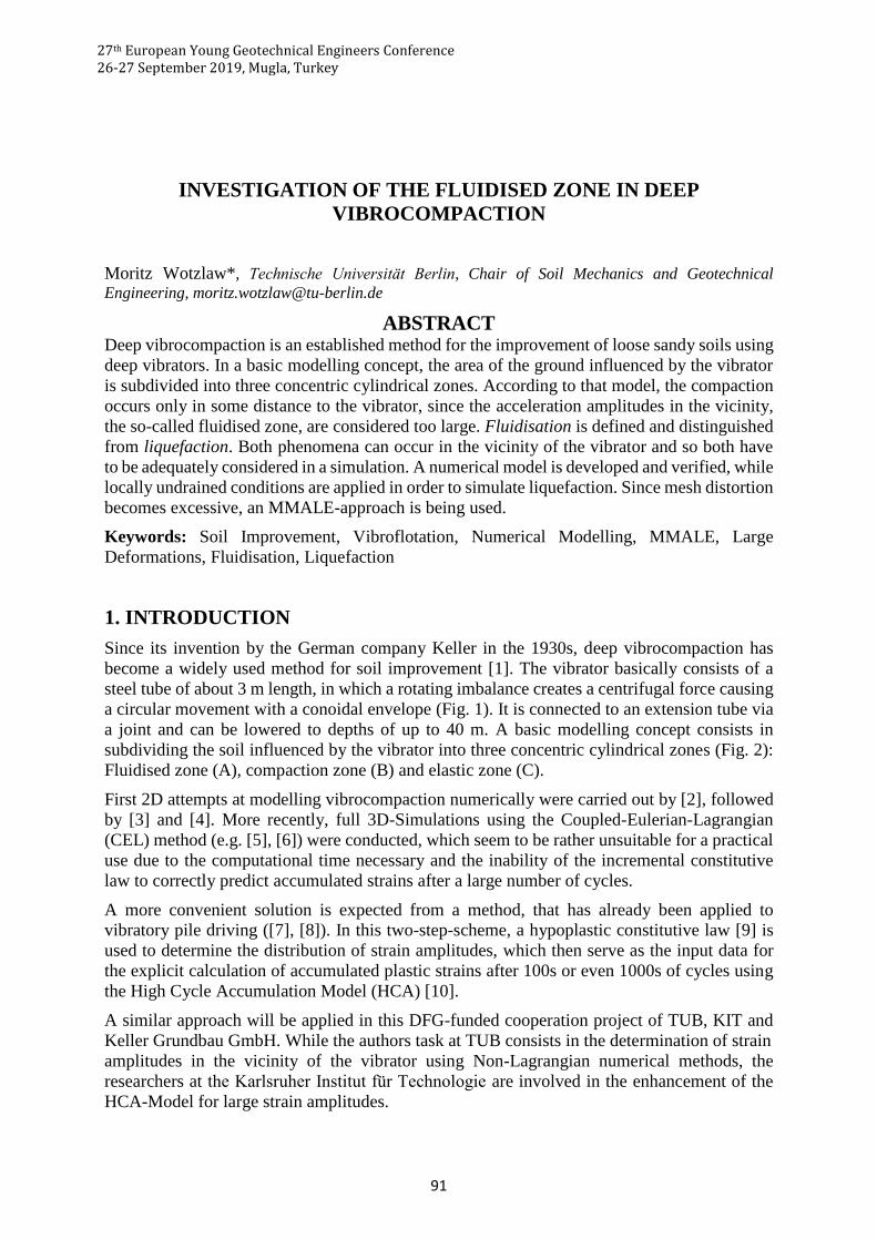
Since its invention by the German company Keller in the 1930s, deep vibrocompaction has

become a widely used method for soil improvement [1]. The vibrator basically consists of a

steel tube of about 3 m length, in which a rotating imbalance creates a centrifugal force causing

a circular movement with a conoidal envelope (Fig. 1). It is connected to an extension tube via

a joint and can be lowered to depths of up to 40 m. A basic modelling concept consists in

subdividing the soil influenced by the vibrator into three concentric cylindrical zones (Fig. 2):

Fluidised zone (A), compaction zone (B) and elastic zone (C).

First 2D attempts at modelling vibrocompaction numerically were carried out by [2], followed

by [3] and [4]. More recently, full 3D-Simulations using the Coupled-Eulerian-Lagrangian

(CEL) method (e.g. [5], [6]) were conducted, which seem to be rather unsuitable for a practical

use due to the computational time necessary and the inability of the incremental constitutive

law to correctly predict accumulated strains after a large number of cycles.

A more convenient solution is expected from a method, that has already been applied to

vibratory pile driving ([7], [8]). In this two-step-scheme, a hypoplastic constitutive law [9] is

used to determine the distribution of strain amplitudes, which then serve as the input data for

the explicit calculation of accumulated plastic strains after 100s or even 1000s of cycles using

the High Cycle Accumulation Model (HCA) [10].

A similar approach will be applied in this DFG-funded cooperation project of TUB, KIT and

Keller Grundbau GmbH. While the authors task at TUB consists in the determination of strain

amplitudes in the vicinity of the vibrator using Non-Lagrangian numerical methods, the

researchers at the Karlsruher Institut für Technologie are involved in the enhancement of the

HCA-Model for large strain amplitudes.

27th European Young Geotechnical Engineers Conference

26-27 September 2019, Mugla, Turkey

92

Figure 1. Schematic of deep vibrocompaction (left) and Modelling concept: fluidised zone

(A), compaction zone (B) and elastic zone (C) (right, both after [1])

In-situ data obtained at construction sites by Keller Grundbau GmbH will be used for validating

the numerical results.

2. MODELLING THE SOIL BEHAVIOR

In this chapter the theoretical background for the soil mechanical processes is briefly

introduced.

2.1. Constitutive Model

The constitutive model applied in the numerical FE-simulations with explicit time integration

is the well-known Hypoplasticity with intergranular strains [9]. The existing implementation

by Mašín [12] was incorporated into the LS-DYNA UMAT using an interface written by

Bakroon et. al. [13].

2.2. Locally Undrained Conditions

Since vibrocompaction is often used in soils where groundwater is present, a consideration of

porewater is necessary. As stated in [14], locally undrained conditions are obtained by

neglecting the porewater flow in a water-saturated soil, which means that volumetric strain

occurs only due to a compression of the pore fluid.

With the rate form of Terzaghi’s principle of effective stress, the locally undrained approach

can be implemented into any material stress-point routine by simply adding the porewater

pressure to the effective stress tensor 𝝈′̇ , computed with the given constitutive law:

�̇� = 𝝈′̇ + �̇�𝑰 (1)

With

being the rate of porewater pressure, calculated from the rate of volumetric strain 𝜀v̇, the bulk

modulus of the pore fluid 𝐾f and the porosity 𝑛.

extension tube

joint

vibratorfins (preventing

rotation around

vertical axis)

path of vibrator

motion

settlement funnel

ground level

Vibrator cross section

rotating imbalance

centrifugal force

AB

C

�̇� = 𝜀v̇

𝐾f

𝑛 (2)

27th European Young Geotechnical Engineers Conference

26-27 September 2019, Mugla, Turkey

93

2.3. Liquefaction and Fluidisation

Two phenomena may strongly influence the soil behavior in Zone A and B: Liquefaction

whenever pore water is present and fluidisation even if the soil is completely dry. While both

of them are characterized by a decrease of shear strength and describe the fact that in this state

the soil behaves like a viscous fluid, the mechanisms involved are not naturally the same.

Liquefaction is a rather well-understood phenomenon in a loose saturated granular soil under

cyclic loading. The induced compactive grain rearrangement can’t be directly transferred to a

volumetric compression because of the present interstitial water and causes a decrease of

effective stress and consequently of shear strength instead. Given that the total stress is constant,

this leads to an increase of porewater pressure.

Fluidisation on the other hand is not well-established in the world of geotechnical engineering.

It may be described as a reduction of shear strength and change of density caused by large

acceleration amplitudes. Although it has been the subject of numerous experimental

investigations in the past (an overview can be found in [16]) it has not yet been included in a

constitutive law to be implemented into common numerical methods like the FEM. Besides the

influence on shear strength it was found, that vertical vibrations with large accelerations cause

dilation, while horizontally vibrations tend to compact the fluidised granular matter.

3. NUMERICAL MODEL

The current numerical model is a straightforward application of the modelling concept in Fig.

1. Since the essential soil mechanical processes are expected to occur in the horizontal plane,

the soil is modelled as a pseudo-two-dimensional disc composed of 3D elements. According to

[3] and [4] this is a justifiable compromise between full 3D- and oversimplified plane-strain-

models.

3.1. Numerical Method

In the immediate vicinity of the vibrator, large soil deformations are expected. This is especially

true, when the shear strength is decreased by liquefaction under undrained conditions. The

application of numerical methods capable of handling large deformations is therefore necessary.

In a Lagrange formulation the material is fixed to the computational mesh and any material

deformation causes mesh deformation. By contrast in a Eulerian formulation, the mesh is fixed

in space and the material may move freely through it. ALE formulations combine the

advantages of both views by introducing a reference domain, which is used to independently

describe mesh and material motion [18].

In most numerical implementations, a three-step calculation scheme is applied, consisting of a

Lagrange step (mesh deforms with material), rezoning step (mesh gets smoothed while the mesh

topography is preserved) and advection step (the material “flows” relative to the rezoned mesh

in order to retrieve the material state after the Lagrange step). ALE formulations are well suited

for the application in geotechnical problems involving large deformations.

3.2. Geometry

The geometry is pictured in Fig. 2. For verification, the same geometry and model size as in [4]

is being adopted. The disc has a radius of 15 m and a depth of 0.5 m. The inner hole containing

the vibrator has a diameter of 0.4 m.

27th European Young Geotechnical Engineers Conference

26-27 September 2019, Mugla, Turkey

94

3.3. Soil Properties

The hypoplastic parameters for the soil in Tab. 1 are taken from [4] with an initial void ratio of

0.85. With a given grain density of 2.65 g/cm³, an initial dry density of 1.43 g/cm³ is obtained.

The initial stress state is taken as a 𝐾0-state with 𝐾0 = 0.463.

Table 1. Parameters for Hypoplasticity with intergranular strains

𝝋𝒄 𝒉𝒔 𝒊𝒏 𝑴𝑷𝒂 𝒏 𝒆𝒅𝟎 𝒆𝒄𝟎 𝒆𝒊𝟎 𝜶 𝜷 𝑹 𝒎𝑹 𝒎𝑻 𝜷𝒓 𝝌

32.5° 591 0.5 0.577 0.874 1.005 0.12 1.0 10-4 2.9 1.45 0.2 6.0

3.4. Boundary Conditions

The soil disc is fixed in horizontal (x- and y-) directions. The horizontal boundary surfaces are

provided with viscous boundaries following the approach of [15] for minimizing wave

reflection.

Although the choice of the “correct” vertical boundaries is not obvious, for the sake of verifying

the basic numerical model, pure stress boundaries are applied analogously to [4]. Since the

modelled depth of the soil disc is 14.5 m to 15 m below ground level, the vertical stresses are

given by 𝜎𝑧,𝑡 = 203 𝑘𝑁/𝑚² at the top and 𝜎𝑧,𝑏 = 210 𝑘𝑁/𝑚² at the bottom.

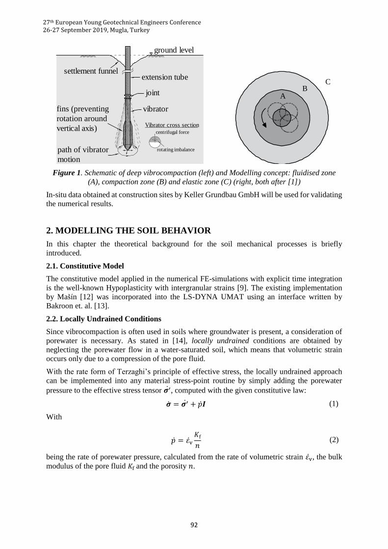
Figure 2. Disc shaped soil model (left, top view) and vibrator model with rotating imbalance

(right)

3.5. Vibrator Model

For reproducing the in-plane movement of the vibrator as realistic as possible, it is modelled as

a tube of rigid solid elements inside of which a lumped mass rotating on a disc composed of

rigid shell elements causes a circular movement (Fig. 2, right). By coupling the translational

DOFs from tube and the disc’s middle node, this motion is transferred to the tube, reproducing

the imbalance-driven motion of the vibrator.

Spring elements are attached to the vibrators center, restraining the movements to a circular

path of a defined amplitude, which can be determined by the quotient of centrifugal force and

spring stiffness.

With a centrifugal force of 𝐹 = 700 𝑘𝑁 and a spring stiffness of 𝑘 = 1 ∙ 105 𝑘𝑁/𝑚 a

displacement amplitude of 𝑢𝑣𝑖𝑏 = 7 𝑚𝑚 (in the air) is obtained which is approximately the

mean nodal displacement amplitude in [4].

Modelling the soil-vibrator interface is achieved via the use of a penalty contact algorithm.

x

y

z Viscous boundaries

SoilPrescribed rotational

velocity

Lumped mass

Vibrator tube

Rotating disc

Spring elements

Vibrator modelSoil model

27th European Young Geotechnical Engineers Conference

26-27 September 2019, Mugla, Turkey

95

4. NUMERICAL RESULTS

After verifying the Lagrange model, the influence of interface friction and the size of Zone A

is discussed. Local undrained conditions are applied for modelling liquefaction.

4.1. Verification of Lagrange Model

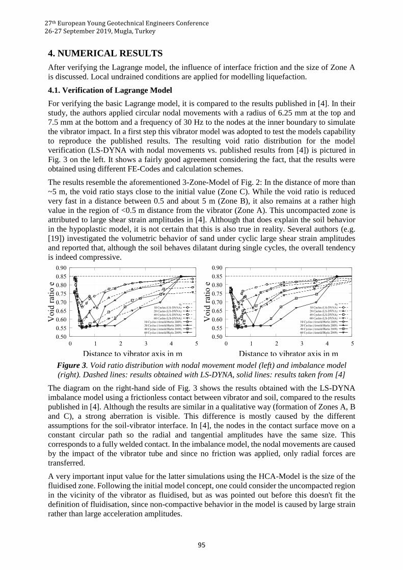
For verifying the basic Lagrange model, it is compared to the results published in [4]. In their

study, the authors applied circular nodal movements with a radius of 6.25 mm at the top and

7.5 mm at the bottom and a frequency of 30 Hz to the nodes at the inner boundary to simulate

the vibrator impact. In a first step this vibrator model was adopted to test the models capability

to reproduce the published results. The resulting void ratio distribution for the model

verification (LS-DYNA with nodal movements vs. published results from [4]) is pictured in

Fig. 3 on the left. It shows a fairly good agreement considering the fact, that the results were

obtained using different FE-Codes and calculation schemes.

The results resemble the aforementioned 3-Zone-Model of Fig. 2: In the distance of more than

~5 m, the void ratio stays close to the initial value (Zone C). While the void ratio is reduced

very fast in a distance between 0.5 and about 5 m (Zone B), it also remains at a rather high

value in the region of <0.5 m distance from the vibrator (Zone A). This uncompacted zone is

attributed to large shear strain amplitudes in [4]. Although that does explain the soil behavior

in the hypoplastic model, it is not certain that this is also true in reality. Several authors (e.g.

[19]) investigated the volumetric behavior of sand under cyclic large shear strain amplitudes

and reported that, although the soil behaves dilatant during single cycles, the overall tendency

is indeed compressive.

Figure 3. Void ratio distribution with nodal movement model (left) and imbalance model

(right). Dashed lines: results obtained with LS-DYNA, solid lines: results taken from [4]

The diagram on the right-hand side of Fig. 3 shows the results obtained with the LS-DYNA

imbalance model using a frictionless contact between vibrator and soil, compared to the results

published in [4]. Although the results are similar in a qualitative way (formation of Zones A, B

and C), a strong aberration is visible. This difference is mostly caused by the different

assumptions for the soil-vibrator interface. In [4], the nodes in the contact surface move on a

constant circular path so the radial and tangential amplitudes have the same size. This

corresponds to a fully welded contact. In the imbalance model, the nodal movements are caused

by the impact of the vibrator tube and since no friction was applied, only radial forces are

transferred.

A very important input value for the latter simulations using the HCA-Model is the size of the

fluidised zone. Following the initial model concept, one could consider the uncompacted region

in the vicinity of the vibrator as fluidised, but as was pointed out before this doesn't fit the

definition of fluidisation, since non-compactive behavior in the model is caused by large strain

rather than large acceleration amplitudes.

27th European Young Geotechnical Engineers Conference

26-27 September 2019, Mugla, Turkey

96

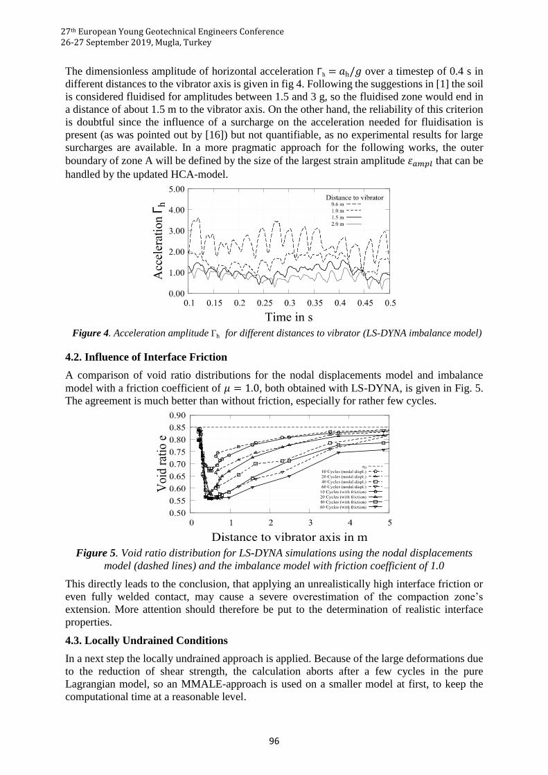
The dimensionless amplitude of horizontal acceleration Γh = 𝑎h/𝑔 over a timestep of 0.4 s in

different distances to the vibrator axis is given in fig 4. Following the suggestions in [1] the soil

is considered fluidised for amplitudes between 1.5 and 3 g, so the fluidised zone would end in

a distance of about 1.5 m to the vibrator axis. On the other hand, the reliability of this criterion

is doubtful since the influence of a surcharge on the acceleration needed for fluidisation is

present (as was pointed out by [16]) but not quantifiable, as no experimental results for large

surcharges are available. In a more pragmatic approach for the following works, the outer

boundary of zone A will be defined by the size of the largest strain amplitude 𝜀𝑎𝑚𝑝𝑙 that can be

handled by the updated HCA-model.

Figure 4. Acceleration amplitude Γh for different distances to vibrator (LS-DYNA imbalance model)

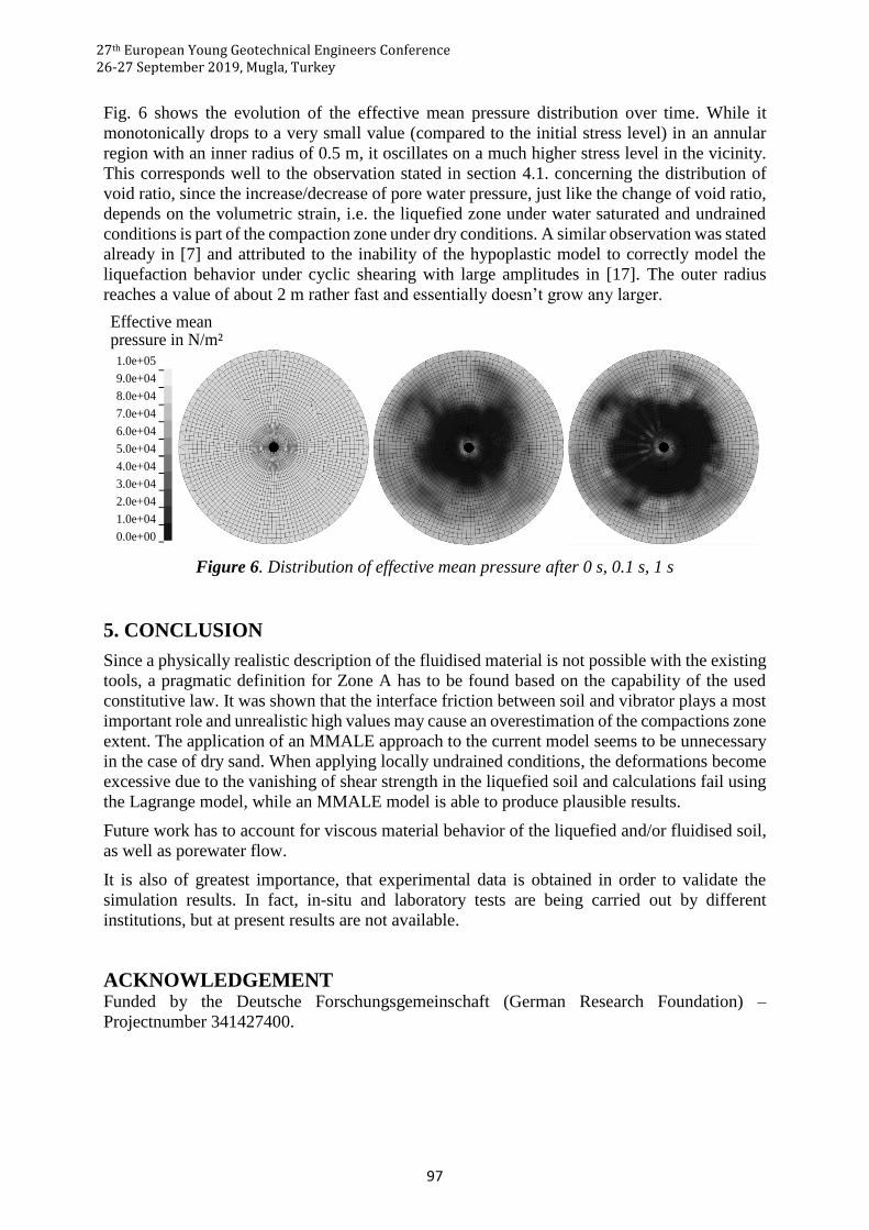
4.2. Influence of Interface Friction

A comparison of void ratio distributions for the nodal displacements model and imbalance

model with a friction coefficient of 𝜇 = 1.0, both obtained with LS-DYNA, is given in Fig. 5.

The agreement is much better than without friction, especially for rather few cycles.

Figure 5. Void ratio distribution for LS-DYNA simulations using the nodal displacements

model (dashed lines) and the imbalance model with friction coefficient of 1.0

This directly leads to the conclusion, that applying an unrealistically high interface friction or

even fully welded contact, may cause a severe overestimation of the compaction zone’s

extension. More attention should therefore be put to the determination of realistic interface

properties.

4.3. Locally Undrained Conditions

In a next step the locally undrained approach is applied. Because of the large deformations due

to the reduction of shear strength, the calculation aborts after a few cycles in the pure

Lagrangian model, so an MMALE-approach is used on a smaller model at first, to keep the

computational time at a reasonable level.

27th European Young Geotechnical Engineers Conference

26-27 September 2019, Mugla, Turkey

97

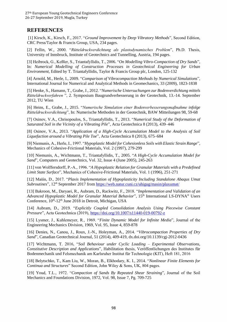
Fig. 6 shows the evolution of the effective mean pressure distribution over time. While it

monotonically drops to a very small value (compared to the initial stress level) in an annular

region with an inner radius of 0.5 m, it oscillates on a much higher stress level in the vicinity.

This corresponds well to the observation stated in section 4.1. concerning the distribution of

void ratio, since the increase/decrease of pore water pressure, just like the change of void ratio,

depends on the volumetric strain, i.e. the liquefied zone under water saturated and undrained

conditions is part of the compaction zone under dry conditions. A similar observation was stated

already in [7] and attributed to the inability of the hypoplastic model to correctly model the

liquefaction behavior under cyclic shearing with large amplitudes in [17]. The outer radius

reaches a value of about 2 m rather fast and essentially doesn’t grow any larger.

Figure 6. Distribution of effective mean pressure after 0 s, 0.1 s, 1 s

5. CONCLUSION

Since a physically realistic description of the fluidised material is not possible with the existing

tools, a pragmatic definition for Zone A has to be found based on the capability of the used

constitutive law. It was shown that the interface friction between soil and vibrator plays a most

important role and unrealistic high values may cause an overestimation of the compactions zone

extent. The application of an MMALE approach to the current model seems to be unnecessary

in the case of dry sand. When applying locally undrained conditions, the deformations become

excessive due to the vanishing of shear strength in the liquefied soil and calculations fail using

the Lagrange model, while an MMALE model is able to produce plausible results.

Future work has to account for viscous material behavior of the liquefied and/or fluidised soil,

as well as porewater flow.

It is also of greatest importance, that experimental data is obtained in order to validate the

simulation results. In fact, in-situ and laboratory tests are being carried out by different

institutions, but at present results are not available.

ACKNOWLEDGEMENT Funded by the Deutsche Forschungsgemeinschaft (German Research Foundation) –

Projectnumber 341427400.

0.0e+00

3.0e+04

2.0e+04

1.0e+04

4.0e+04

5.0e+04

6.0e+04

7.0e+04

8.0e+04

9.0e+04

1.0e+05

Effective meanpressure in N/m²

27th European Young Geotechnical Engineers Conference

26-27 September 2019, Mugla, Turkey

98

REFERENCES

[1] Kirsch, K., Kirsch, F., 2017. “Ground Improvement by Deep Vibratory Methods”, Second Edition,

CRC Press/Taylor & Francis Group, USA, 234 pages.

[2] Fellin, W., 2000. “Rütteldruckverdichtung als plastodynamisches Problem”, Ph.D. Thesis,

University of Innsbruck, Institute of Geotechnics and Tunnelling, Austria, 194 pages.

[3] Heibrock, G., Keßler, S., Triantafyllidis, T., 2006. “On Modelling Vibro-Compaction of Dry Sands”,

In: Numerical Modelling of Construction Processes in Geotechnical Engineering for Urban

Environment, Edited by T. Triantafyllidis, Taylor & Francis Group plc, London, 125-132

[4] Arnold, M., Herle, I., 2009. “Comparison of Vibrocompaction Methods by Numerical Simulations”,

International Journal for Numerical and Analytical Methods in Geomechanics, 33 (2009), 1823-1838

[5] Henke, S., Hamann, T., Grabe, J., 2012. “Numerische Untersuchungen zur Bodenverdichtung mittels

Rütteldruckverfahren ”, 2. Symposium Baugrundverbesserung in der Geotechnik, 13.-14. September

2012, TU Wien

[6] Heins, E., Grabe, J., 2015. “Numerische Simulation einer Bodenverbesserungsmaßnahme infolge

Rütteldruckverdichtung”, In: Numerische Methoden in der Geotechnik, BAW Mitteilungen 98, 59-68

[7] Osinov, V.A., Chrisopoulos, S., Triantafyllidis, T., 2013. “Numerical Study of the Deformation of

Saturated Soil in the Vicinity of a Vibrating Pile”, Acta Geotechnica 8 (2013), 439–446

[8] Osinov, V.A., 2013. “Application of a High-Cycle Accumulation Model to the Analysis of Soil

Liquefaction around a Vibrating Pile Toe”, Acta Geotechnica 8 (2013), 675–684

[9] Niemunis, A., Herle, I., 1997. “Hypoplastic Model for Cohesionless Soils with Elastic Strain Range”,

Mechanics of Cohesive-Frictional Materials, Vol. 2 (1997), 279-299

[10] Niemunis, A., Wichtmann, T., Triantafyllidis, T., 2005. “A High-Cycle Accumulation Model for

Sand”, Computers and Geotechnics, Vol. 32, Issue 4 (June 2005), 245-263

[11] von Wolffersdorff, P.-A., 1996. “A Hypoplastic Relation for Granular Materials with a Predefined

Limit State Surface”, Mechanics of Cohesive-Frictional Materials, Vol. 1 (1996), 251-271

[12] Mašín, D., 2017. “Plaxis Implementation of Hypoplasticity Including Standalone Abaqus Umat

Subroutines”, 12th September 2017 from https://web.natur.cuni.cz/uhigug/masin/plaxumat/

[13] Bakroon, M., Daryaei, R., Aubram, D., Rackwitz, F., 2018. “Implementation and Validation of an

Advanced Hypoplastic Model for Granular Material Behavior”, 15th International LS-DYNA® Users

Conference, 10th-12th June 2018 in Detroit, Michigan, USA

[14] Aubram, D., 2019. “Explicitly Coupled Consolidation Analysis Using Piecewise Constant

Pressure”, Acta Geotechnica (2019), https://doi.org/10.1007/s11440-019-00792-z

[15] Lysmer, J., Kuhlemeyer, R., 1969. “Finite Dynamic Model for Infinite Media”, Journal of the

Engineering Mechanics Division, 1969, Vol. 95, Issue 4, 859-878

[16] Denies, N., Canou, J., Roux, J.-N., Holeyman, A., 2014. “Vibrocompaction Properties of Dry

Sand”, Canadian Geotechnical Journal, 51 (2014), 409-419, dx.doi.org/10.1139/cgj-2012-0436

[17] Wichtmann, T. 2016, “Soil Behaviour under Cyclic Loading – Experimental Observations,

Constitutive Description and Applications”, Habilitation thesis, Veröffentlichungen des Institutes für

Bodenmechanik und Felsmechanik am Karlsruher Institut für Technologie (KIT), Heft 181, 2016

[18] Belytschko, T., Kam Liu, W., Moran, B., Elkhodary, K. I., 2014. “Nonlinear Finite Elements for

Continua and Structures” Second Edition, John Wiley & Sons, UK, 804 pages.

[19] Youd, T.L., 1972. “Compaction of Sands By Repeated Shear Straining”, Journal of the Soil

Mechanics and Foundations Division, 1972, Vol. 98, Issue 7, Pg. 709-725