Page 1
Scholars' Mine Scholars' Mine
Masters Theses Student Theses and Dissertations
1965
Investigation of the use of optics in the analysis of structures Investigation of the use of optics in the analysis of structures
Jimmy D. Hahs
Follow this and additional works at: https://scholarsmine.mst.edu/masters_theses
Part of the Civil Engineering Commons
Department: Department:
Recommended Citation Recommended Citation Hahs, Jimmy D., "Investigation of the use of optics in the analysis of structures" (1965). Masters Theses. 5703. https://scholarsmine.mst.edu/masters_theses/5703
This thesis is brought to you by Scholars' Mine, a service of the Missouri S&T Library and Learning Resources. This work is protected by U. S. Copyright Law. Unauthorized use including reproduction for redistribution requires the permission of the copyright holder. For more information, please contact [email protected] .
Page 2
INVESTIGATION OF TifE USE OF OPTICS
IN THE ANALYSIS OF STRUCTURES
by
JilvU1Y DEAN HAllS
A
THESIS
submitted to the faculty of the
ID~IVERSITY OF NISSOURI AT ROLLA
in partial fulfillment or the requirements for the
Degree of
HASTER OF SCIENCE IN CIVIL ENGINEERING
Rolla, Missouri
1965
APPROVED BY
Page 3
ABSTRACT
This study \vas made to determine the feasibility of
the use of optics in the analysis of structures. Since
the curvature of a beam due to a loading condition is a
function of the moment, a measure of this curvature is a
measurement of the moment.
This study used the relationship between object size
and image size formed by a concave or convex reflective
surface to determine the radius of curvature and the moment
at the point.
Overhanging simply supported beams of plexiglass with
concentrated loads at various positions \vere used to det:on
strate the developed optical theory. Optical measurements
i.vere taken on the beams and the data plotted to obtain
moment diagrams and inflection points which were compared
with the results obtained by the use of sta tics. 1ne com
parisons \vere within tolerable limits and shm·Ted that the
optical method is feasible.
ii
Page 4
iii
A CI'JT 0\'JLEDGl<:ET·TT
The author ·~:~ishes to express his sincere than1w to
Dr. J. H. Senne, Jr., Chairman of the Civil Eneineering
Department, for introducing the subject and giving constant
encouragement and advice.
The author is also appreciative of the help given to
him by N. L. Brown, Instructor of Civil Engineering, in
assembling the instrumentation. The fine craftsmanship of
J. Smith is also appreciated.
Page 5
TABLE OF CONTENTS
ABS'fiti\.CT •••••••••••••••••••••••••••••••••••••••••••
A CKN 0 ~oJL .EDGHENT •••••••••••••••••••••••••••••••••••••
LIST OF FI GURES ••••••••••••••••••••••••••••••••••••
LIST OF TABLES ••••••••••••••••••••• . •••••••••••••••
LIST OF SYHBOLS ••••••••••••••••••••••••••••••••••••
I. INTRODUCTION ••••••••••••••••••••••••••••••
II. REVIEvl OF LITE:HA1\JHE ••••••••••••••••••••••
III. DIS CUSS ION
3-1
3-2
3-3
General Theory ••••••••••••••••••••••
Derivation of General Relationship
for Location of Inflection Points •••
Derivation of General Relationships
Required to Dra1.v the N Diagram •••••• EI
3-4 Derivation of General Relationships
Required to Draw the Homent Diagram.
IV. DEHIVATION OF EQUATION FOR EXPEHHIENTAL
INSTHUl·IEUTATION ••••••••••••••••••••••••••
v. TEST APPA~~AT : ~ •••••••••••••••••••••••••••
VI. TES'l1 Pl\OCEIJ .... :J.\E •••••••••••••••••••••••••••
VII. DISClJSSIOl~ OF'I : ~~ :~S ~JL1.lS ••••••••••••••••••••
VIII. COI'·J CIJ TJS I 0 l~ S ••••••••••••••••••••••••••••••
IX. HECOI-.. il·lENDAT I ONS ••••••••••••••••••••••••••
APPENDICES
I • • • • • • • • • • • • . • • • . • • • • • . • • • • .. • .. • . • . • .. . . . . . . II ••............•..............•...•...•.•....•
iv
Page
ii
iii
vi
ix
X
1
2
4
8
9
9
17
21
26
?7
58
60
Page 6
'I'ADLE OF COli'I'K!'i'S (continued.)
BIBLIOGHAPIIY. • • • • • • • • • • • • • • • • • • • • • • • • • • • • • • • • • • • • • •
VI TA •• •••••••.•••••••••••••••••••••• 41 ••••••••••••••
v
Page
69
70
Page 7
LIST OF li'IGUHES
Figure
1 • Concave curvatu.re ••••••••••••••••••••••••••••
2. Convex curvature •••••••••••••••••••••••••••••
3. Ellipsoidal segment of a beam ••••••••••••.•••
4. Elements of a cylindrical mirror •••••••••••••
5. Image formed of an object by a concave
mirror when sis less than f •••••••••••••••••
6. Image formed of an object by a convex
mirror • ....•.....•...••.......•..........••..
7. Formation of an inflection point •••••••••••••
8. Image formed of an object by a thin lens •••••
9. Images formed by instrumentation •••••••••••••
1 o. r··licrometer' lens and 0 bj ect ••••••••••••••••••
1 1 •
12.
13.
14.
15.
Image as seen through the micrometer •••••••••
Supporting frame and carriage ••••••••••••••••
Adjusting screws of the carriage •••••••••••••
Instrumentation for runs 1 '
2 and 3 ••••. •..••
Instrumentation for rlllls 4, 5 and 6 • •..••.•.•
16. Image measurement ••••••••••••••••••••••••••••
16(a). Distorted images •••••••••••••••••••••••••••••
17. Channel support for zero readings for
rlUls 4, 5 and 6 •••••••••••••••••••••••••••••••
18. y 0' 1 y 11 2 _..;;:.._..,..,...._ x 10 versus moment - run 1 •••••••••• yli
19. Location of the images formed by the lens
for flat, concave and convex beruas •••••••••••
vi
Page
11
11
12
13
14
1 5
16
19
20
23
23
24
25 29
30
31
32
33
4o
41
Page 8
vj_i
LIST Uti' F IG!.JHES (continued)
FigLJ.re
20. Y~ - Y11 x 102 versus moment - run 2....... 42
y''
21. Yo- Y" x 102 versus moment- r t.m 3....... 43
y"
22. Loading condition, moment diagram and
elastic curve- run 4..................... 44 23. Loading condition, moment di <tgrarl and
ela stic c urve - rw1 5..................... 45 24. Loading condition, Dornent diagrau and
elastic cur ve - run 6. • • • • • • • • • • • • • . • • • . • • ~-6
25. Initial and loaded readings versus distance-
rur1 4.............. . . . . . . . . . . . . . . . . . . . . . . . lr9
26 . Experim(.;ntal and theoretical nonents versus
distance - rt.m 5.......................... 49
27. Initial and loaded readings vers us distnnce-
rur1 5. . . . . . . . . . . . . . . . . . . . . . . . . . . . . . . . . . . . . 50
28 . Initial a nd loaded readings ver sus distance-
rtm 6.... . . . . . . . . . . . . . . . . . . . . . . . . . . . . . . . . . 50
29. Expe:cir:1e.::1t a l and t heorc t j_ cal ElOJ:lent s v e;_--s us
dista.nce- rLUl 5..... ................. .... 54-30. Exps r j_u en. tal and t h eor e tj_cal mor:en ts ve r s us
dis tt1 ~:1ce - run 6.......................... 55
31 • Cantilevered beaJJl . • • • • • • • • • • • • • • • • • • • • • • • • 62
32. Def l ection versus time.................... 64
33. Loading conditions- cases 1, 2 C:l.J.'1d 3 •••.• 65
Page 9
viJi
LIST OF FIG UHES (continued)
Figure Page
34. Deflection versus load- cases 1, 2 and
average................................... 67
35. Deflection versus load- case 3........... 68
Page 10
ix
LIST OF TABLES
Table Page
I. Loaded Readings- Run 1................. 38
II. Loaded Readings- Run 2................. 38
III.
IV.
v. VI.
VII.
VIII.
IX.
x.
Loaded Readings- Run 3 •••••••••••••••••
Initial Readings -Runs 4, 5 and 6 ••••••
Loaded Readings - Huns 4, 5 and 6 •••••••
Experimental Homent Run 4 •••••••••••••
Experimental Homent- Run 5 ••••.•••••••• Experimental Noment RWl. 6 •••••••••••••
Creep Deflection ••••••••••••••••••••••••
Deflection of Cantilever Beams ••••••••••
39
47
48
51
52
53 63
66
Page 11
X
LIST OF SYHBOLS
The symbols are defined '\·!here they first occur in the
text and are listed here in alphabetical orc,er for convenience.
c Hatio of ll.s to s 2 E Modulus of elasticity (gm/cm )
F Focal point
f Focal distance (em)
I Homent of inertia (cm4 )
L Span length (em)
H Homent (gm-cm)
m Magnification of the beam
m_ l·lagnification of the lens L
P Concentrated load (gm)
R Radius of curvature of the elastic curve (em)
Rm Radius of curvature of the mirror (em)
s Distance from the object to the beam (em)
s 1 Distance from the beam to the image it formed (em)
s1 Distance from the lens to the image formed by the
beam (em)
sL Distance from the lens to the image it formed (en )
As Distance from the object to the lens (em)
w Uniform load (gm/cm)
y Object size (em)
y 1 Size of the image of the beam (em)
y 11 Size of the image of the lens for any load (YJicro
meter divisions)
Page 12
xi
LIST OF S:Ll-lBOLS (continued)
y11 Size of the image of the lens vlhen the moment is 0
zero (micrometer divisions)
z Distance from the top of the 1Jeam to the neutral
axis (em)
a Deflection (em)
Page 13
1
I. INTHODUCTION
There are many methods of analyzing structures available
to the engineer. One of the most common methods is by the
use of equations derived from statics and mechanics of ma
terials '"hich are especially convenient '\vhen the structure
is statically determinate. The solution of these equations
for highly statically indeterminate structures becomes diffi
cult and in some cases almost impossible.
A second raethod of analysis is by the use of models
which, one might sa:;~, is a field of its mvn. There are
many types of models and many approaches which can be used
in model analysis. In general, the use of models is of par
ticular value ,.,hen the structure is either highly indeter
minate or has many variables.
Since the curvature of a beara due to a loading system
is a function of the moment, a determination of the curva
ture is a means of determining the moment in the beam.
The shape of the image of an object formed by a reflective
surface is a fLmction of the shape (curvature) of the su1·face.
Thus, the relationship of thG shape of the image :Ls a function
of the moment if the curvature is due to the applicatj_on or
a moment to a reflective beam.
This study -vms made to determine the relationship bet\·Jeen
the moment and the shape of the imac; e and to nH.'1.ke an experi
mental investigation to check the feasibility of this re
lationship.
Page 14
2
Optics are used in conjw1ction ·vri th mechanical levers
as strain ga ges. These gages are very precise and sensitive.
The general procedure using mechanical-optical stra in gE~t;es
is to secure a reflect i ve pivoted member or lever in the
gage. As the structure is deformed, t he lever i s r o tateC
due to a change bet1veen the gaging points causing the attached
reflec t ive surface to rota te. A collimated beau of li t;:ht is
reflected from the gage to a scale; the motion of the beam
indicates t he def ormation of the gage length. To increa s e
the magnification of the movement, a telescope can be used(1).
'!The only p urely optical strain gages are of the in
terferometer type" (1). This type of gage uses t\w parallel
flat ontica l plates f asten ed sec u.rely to t h e structure with
out ,,rarping. A monochromatic J.ight beam is passeC. through
a half-silvered mirr or normal to t he o:ptica l plat es. The
interference fringes are observed with a telescope through
the back side o f the mirror.
As the deformation of the structure occurs, t he inter-
f erence rinr;s are counted <: s the:l Jr;ove pc:::.st a n es t a bl i shed
point on one of the optica l f lats. dith each move~ent of
one compl ete f ringe past t he referenc e malce, the op ti cal
f l a ts have moved one-half of one v.J.~;_ v e length o.f t h e l i :_,ht
used. With proper adjustment,tlds ga ge can be very sensitive.
"The use of optical fla ts, or t:!:1e i n t e r fermome t cr as a strain
gage, is the closest to t he absolut e meas ure1!Ien t, of stra :i.n
that we are able to attain,(1).
Page 15
A..t1.other method of measuring deformations of a nodel
is the Beggs Deformeter \'lhich uses a micrometer r.nicroscope
to r;leasurc the movement at one point due to a l:nmvn change
in the conditions at an.other point. The la'\-T of reciprocal
deflections can be applied to analyze the model (2).
One useful method of solving certain structural
problems is the use of ::1embrane analogies. This method
3
uses the contours of the shape of a thin membrane under
pressure on one side to be analogous to a certain structural
phenomenon. One method of measuring these contours is of
interest in the follm.;ing study. The method is an application
of optical and geometrical principles. A light source is
located at a known elevation above the memb:bane boun.6ary
or some convenient reference plane. The light is po~;i tioned
so that the reflection fror:1 the mem"L:rane is observed along
a line that intersects the vertical line through the light
source. By measuring certain distances and angles, the
slope of the membrane at the point of reflection and the
elevation of the membrane at that point may be cor!lputed ( 1).
Page 16
III. DISCUSSION
3-1 General Theory
The curvature at any point in a beam is a function of
the moment, the modulus of elasticity, a~d the moment of
inertia of the cross-section. For small deflections, this
well-knm·m relationship is given by the follm·ring:
1 = 1·1 'R EY
i.vhere
R = Radius of curvatu.re of the beam,
H = Homent,
E = Nodulus of elasticity, and
I = Homent of inertia.
(Eq. 1)
The loading and elastic curve for the longitudinal
dimension of t1.vo beams are shm·m in Figure 1 and Figure 2.
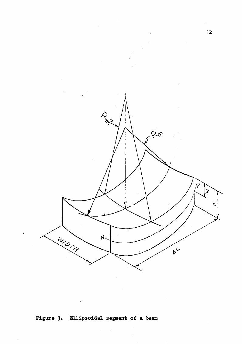
Using a beam that has a reflective surface and taking
a small element of this surface as shovm in Figure 3, an
ellipsoidial mirror is formed. This mirror has a radius
1\n for a segment along the longitudinal axis ·of the beam
and a radius Rro1 for the segment along the transverse axis.
When the beam is loaded so that no torsion is obtained
and the deflection is small, the curvature of the segnent
along the transverse axis approaches zero or the radius
approaches infinity.
This. asswnption allovrs the surface element to be con-
sidered one of cylindrical shape as shown by Figure 4,
'WiLth the radius of the mil"rco.r· equal to the radius o.f' the
Page 17
top surfa ce of the beam and the height of the cylj_nder equal
to the \ITid th of the beam. Although the c urv<:?.t ~u·e o i' the
beam is constant only if E, I, and H are constant, the
curvature for a small ele::nent cc=> .... n. be assurned to be constant.
F'igure 4- shm·rs both concave curvature and convex: curva-
ture.
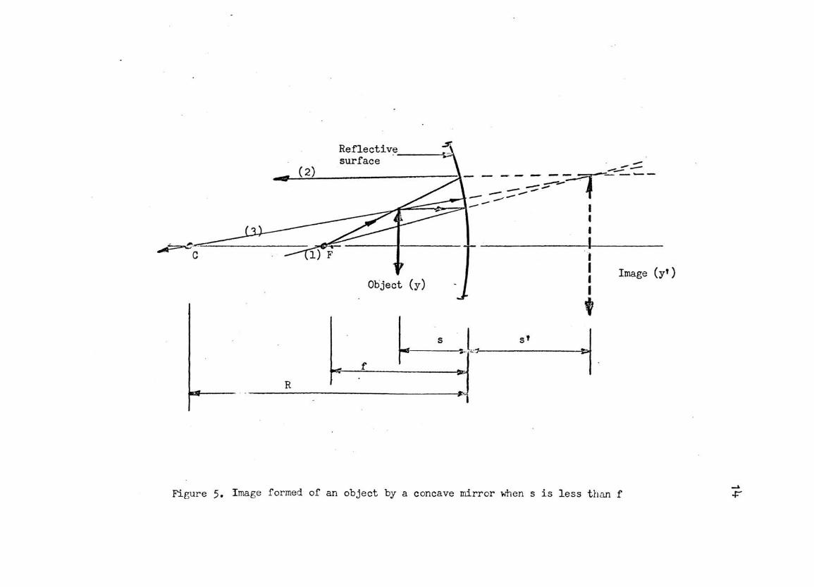
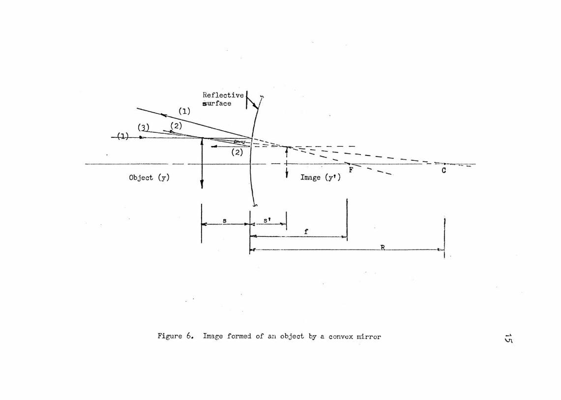
Figures 5 and 6 show the construction for finding the
image formed by a cylindrical concave mirror and convex
mirror, respectively. The procedure for locating lines 1,
2, and . 3 is e~)lained in Appendix I.
The concave mirror represented is of la:q;e radius ~·
The focal distance (f) is given by the follmving:
f = -Rm 2
(Eq. 2)
5
Since 1\n approaches infinity as the curv<,~ ture approaches
zero, the focal distance also approaches infinity as the
curvature approaches zero. When the object y is located
at some distance s between the focal point and the surface
of the mirror, the image yr \dll be at some distance s r on
the opposite side of the surface.
The relation bet,, ... een s, s 1 , and I\n is given by the
follmving:
1 - 1 = ~ (Eq. 3) s s• -m.
The magnification m is given by the follm·ring:
ID : zt: ~I y s (Eq. 4)
Page 18
6
\.Jl1en the following sign convention commonly used by the
optical industry is adopted, the relationship for the focal
distance, radius and the mat;nification can be a~)plied to
convex mirrors C'~S·O ( 3).
1. DravJ all diagrams 1.vi th the incident light traveling
from the left to the right.
2. Object distances s are positive if the object point
lies to the left.
3. Image distances s' are positive if the image lies
to the right of the surface.
4. Radii of curvature 1\n are positive if the center
of curvature lies to the riBht of the surface.
5. Transverse dimensions y and y 1 are positive if
above the axis.
Substituting Eq. 4 into Eq. 5 and rearranging, the
following is obtained:
1 = =1 (y' - ~l I\n 2s y' ( Eq. 5)
Since H is the radius of curvature of the elastic curve
of the bear1 and the elastic curve is located some distance z
below the top surface of the bean (Figure 4-), H is equal
to the radius of the top s urface plus z for a concave surfac e.
Since the radius of the top surf ace is equal to 1:\n' the radius
of the mirror, R is equal to R + z. m
Substituting Rm + z for R in Eq. 1 and rearranging,
the follo'\lling is obtained:
1 R m
= =_;.;M.......,..., EI - zH
(Eq.6)
Page 19
7
EOt:lat; :..n.::..-· T:~q~ • r; ~and 6 rr·i VeS t11e follO''. ng 1 t. . . -- ... _ s - ~ ./ ~ 6~- · ,·.l . re a ~onsrnp;
1 : +1 (y - y I) : J.vl TI 2s y' EI - zH m
(Eq. 7)
Solving Eq. 7 for H, the follouing is obtained:
H = +1 (y- z')EI 1 (Eq. 8) 2s yt . 1-2CY-y1 )
2s y
Since z is a small quantity for raost cases 2s and y - y' Y'
is small, the product \vill be very small. vJi th this assumption,
Eq. 8, reduces to the follm·Ting:
H = + EI ( y - y I )
2s . y1 --(Eq. 9)
From the adopted sign convention and l'igure 5, y, y 1 ,
s an.d s 1 are positive for a concave surface. Also, y' is
larger than y. Thus, for a concave surface the raoment 'Hill
be a negatj_v e ·Hhich establishes the sign convention of com-
pression in the top ·fibers as a result of negative monent.
This sign convention for moment V-Till be used in the remainder
o r the text.
\men Fir,ure 6 is considered, the surface is convex. ,,
The radius of curvature of the convex reflective s u.rf<'l.cc is
H + z (Figure 4). 11hen :;_:~ - z is substituted into 3q. 1
aJ.'ld similar steps are ta!;:en as for conc c.vc su.rf'e.ces, t r.te
follovTing i s obta:Lned:
M = +EI (y- y') 1 y I T1-+-:--z~( ~-r ---y-=-r )
2s y'
(Eq. 10)
\vith the assumption that z (y- y 1 ) is very small, 2s yi
Page 20
.E:q. 9 is obtained for convex, as well as concave s urfaces.
For convex surfaces, y, y', sands' are all positive; but
Figure 6 diagramrn.atically shmvs tha t y' will be less than
8
y, wLich gives the quantity (y- y') a positive sign and
makes the moment obtained from Eq. 9 positive. Thus, the
moment required to obtain convex curvature is positive, vrhich
agrees '\-Ii th t he adopted sign convention that compression in
the top is due to negative moment. Conversely, tension in
the top fibers is a result of positive moment.
Eq. 9 shm,rs that if E, I, s, y and y' are knovm or
measured, the moment at that point can be computed.
3-2 Derivation of General Relationship f or Location of
Inflection Points
Figure 7 illustrates a general loading condition the. t
will produce a..'l inflection point. An infleetion point is
the point at vrhich convex curva tm~e changes to conc .::lve
curvature or vice versa (4). Using the fi rst ca:.::e as sho\.vn
in Figure 7, to the left of the inflection point (convex
curvature) the moment is seen to be positive and to the
right of t he inflection point the moment is negative , or
to the left y' is less than y and to the right y' is grea ter
than y. '£he moment is zero at the inf l e cLLo.n poi:lt.
When Eq. 9 is set equal to zero, it is seen t ha t the
only quantity that can ph,ysically be zero is y - y'. Hence,
y = y 1 at t he inflection point.
Therefore, the inflection point can be found by locating
the point on the beam where y = y 1 •
Page 21
3-3 Derivation oi' General Relationships Heoui:ced to Draw
the H Diagram EI
One convenient method of f inding the deflecti on and
the a'1.gular rot ~ ;. tion is to apply the principles of moment
area. It is desirable in this application to obtain the
l .. I diagram. Er
Referring to Eq. 9 and rearranging, N is given by the EY
follovTing:
H = -1 (y' - y) - - - I EI 2s y . . (Eq. 11)
9
When the object distance is held constant and the above
equation is r ci:lri tten, the f ollovJing i s obtained~
H = K1 (y' - y) liT yl
\vhere K1 = -1 2s
(Eq. 12)
Since H is proporti onal to (y' - y_), a plot of y' - y EI yf yf'
versus distance gives a diagr am tha t is proportional to the
H diagram. EI
3-4 Derivati on of the General Relationship Heg,uiyed to
Draw the Homent Diagram
From Eq. 9 the moment at any point is r; i ven as a ft:mction
of E, I, y', y and s. I f t hese are measured and the f1JJ1ction
plotted versus t he dis t a.nce, the moment diagra:rJ is obtained.
For a beam of constant I and E, Eq. 9 can be re\Iri tten
in the f ollowing f orm:
Page 22
10
H = K2 (1) (;z I - :z) s yf (Eq. 13)
vJhere K2 = -EI ~
If the object is moved parallel to the longitudinal
axis of the beam, s vrill remain constant for small deflections.
Hev1ri ting the above equation, the f ollo\'Ting is obtai ned:
M = K3 ( y t . i y) y (Eq. 14)
Thus, a plot of y' - y versus distance will f~~ ive a yi
diagram whose ordinates are proportional to the moment dia-
gram.
Page 23
Loading condition
Elastic curve
Loacling condition
Elastic curve:
11
figure 1.. Concave curvature
Figure 2. •. Convex curvature:
Page 24
12
Figure 3· Ellipsoidal segment of a beam
Page 25
I· b ~ A-A -
z t
Concave reflective: surface;
Convex refle:cti:ve. surface
0
Figure ~. Elements of a cylindrical rn.irJJor
13
Page 26
( 2)
Reflective ~ surface
-- --- -~.:;::::.. ,.._ - - - -=" ::::--f----- :_-- ---?- =:::>1-- I
I
~~ ~ -----11·-----c
I I
• I
R
Object (y) I I
t I . 1 •• J ~-~'~
~ f ~
,.,,
Image (y')
Figure 5. Image formed of an object by a concave mirror when s is less than f ~
+
Page 27
Reflective surface
, ) .. -=-=-,.. =-------· ~ E t
--Object (y)
7' I
~ s ~--Y
- -- -- -==~-=.---=::--::_-c F - --Image (y')
f
R J I
Figure 6. Image formed of an object by a convex mirror _. V\
Page 28
Loading condition
Homent diagram (gm-cm)
Elastic curve
lt::p=1===;=~ _r_=· =========:::-,
RL t- RR t a .1.. b .j. c ~
Figure 7. Formation of an inflection p~int
16
Page 29
17
IV. DEHIVA'I'ION OF EQ -. JA'.U01'·I FOH EXPEHii.li.!:N'l'Ai. INSThUtiEN'l'ATION
Consider the beam to be a segraent of a cylindr:ical
mirror '\vi th the magnification c;iven by the follmdng:
y I S I
m - - = y s (Eq. 4)
The image formed by the mirror is the object of the
lens. Figure 8 shovrs the formation of an image by a thin
lens. The procedure for the locating lines 1, 2 and 3 is
explained in Appendix I. The magnification of the lens is
where
~ = :Hagnification of the lens,
sL = Image distance of the lens,
s1 = Object diste.nce of the lens,
yu = Image size of the lens, and
y' = Image size of the mirror.
(Eq. 1 5)
Figure 9 shows that s1 = s +As + s 1 = (1 + c + m)s.
\>!hen this is substituted into Eq. 15, the follm1ing is
obtained:
Y'
-si m = c:
1 -c-c-+ 1 + m") s
Y'' (Eq. 16)
\Vhen ym is substitu.ted into Eq. 16 for y' ru1.d rearranc;ed,
the following is obtained:
-(c + 1) m = st + 1
yus (Eq. 17)
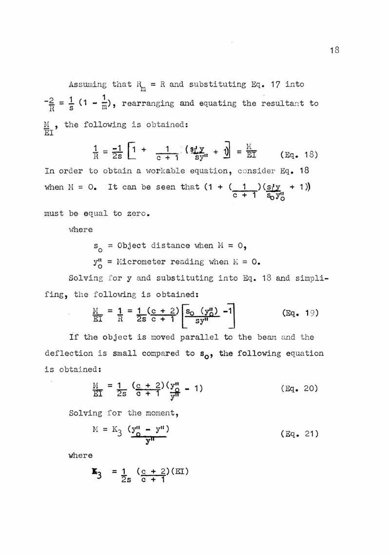
Page 30
Assuming that H = R and substituting Eq. 17 into m
-~ =! (1 - ~), rearranging ru1d equating the resultan t to
H the following is obtained: - ' EI
1 = -1 f1 + H 2s L 1 . {U.Z + J =
c + 1 · SY11 .YJ (Eq. 18)
In order to obtain a \vorkable equation, consider Eq. 18
\vhen H = 0. It can be seen that ( 1 + ( 1 ) (§1..:1. + 1 )) c + 1 SoY'~
must be equal to zero.
vrhere
s0 = Object distance \·Then N = o,
y~ = Hicrometer reading when f.l = 0.
Solving f or y and substituting into Eq. 18 and simpli-
fing, the f ollmring is obtained:
£L = 1 = 1 <c + 2) ~o <to) -11 EI R 2s c + 1 [ syu J (Eq. 19)
If the object is moved parallel to the beam and the
deflection is small compared to s0 , the follO\ving equation
is obtained:
H = 1 ( c + 2) ( y" 1 ) EI 2s c+1 ~-
Solving for the moment,
H = K3 (yu - y") 9
where
= 1 (c + 2)(EI) 2s c + 1
(Eq. 20)
( Eq. 21)
18
Page 31
Object (y)
s
I ~hin lens I '\ '"Y-::: · t I d >/ '-...._ -....._ F 1- z:_~ \ - '*......_. I
~ 'IT;' - ---~-- · '.......... I Image Cy•J r -- --····
---~~, -~ . ---::---
+-----f _____ ....c,:.l~r-----~ ~' --~~ s'
~r~ ~-'1
Figure 8. Ima.ge formed of an object by a thin lens ~
'-0
Page 32
Image formed by the lens
Lens
1
j_ ----~
Object (light source)
Reflective
s
surface of~------------~----------~~--the beam
Image formed by the beam
Figure 9. Images formed by ins trumenta:I;ion
20
Page 33
V. TES'l' APPAHATUS
Figure 10 shows a detail of the micrometer, lens and
the object used in this study. The micror:1eter is the
measuring device used in the Beggs Deformeter. It can
be read directly to the nearest division and vras estimated
to the nearest .5 division for the first group and to the
nearest .2 division for the last group of ru..'1.s. The units
of divisions were substituted directly into Eq. 20 as is
explained in the Test Procedure of this study.
The lens used was the object lens of a solar attach
ment to a transit.
The object used was a 224 light bulb which had its
energy supplied by flashlight batteries. The design pro
duced by this obj ect is shm.m in Figure 11.
The frame and the supporting carriage for the microme
ter are shm.·m in Figure 12. 'l'he frame and carriage \vere
adapted from photogrammetry equipment.
The frame \vas equipped with adjusting scre\vS -vrhich
allowed vertical adjustment and leveling of the track of
the carriage. Shims were placed bet\veen the track and the
frame to establish a vertical plane for the rollers of the
carriage.
21
The carriage \vas equipped with several adjusting scre\·Js
that facilitated the opera tions considerably. These screws
are labeled in Ii''igure 13 and are descrj_ bed as follov.rs.
Page 34
22
Sere\-! one allO\ved the carriage to be moved parallel
to the longi tudional axis of the specimen and in a horizont:ll
plane.
Scre\v two allowed vertical adjustment of the measuring
system.
Screw three allm.ved rotation about an axis parallel to
the transverse axis of the specimen.
Screw four allowed the rotation about an axis parallel
to t he longitudional axis of the specimen.
The specimens used in this stu6.y were made of plexi
glass. The bottoms of each were coated with a black dye to
improve the image formed on the top surface of the specimen
and to eliminate the image formed by the bottom surface of
the specimen.
The specimen used in rtlll 1 was 1/8" X .4n X 15" and
in run 2 was 1/8" X .ti-n X 19. 6" and in rtlll 3 was 1/411 X
.4" X 15".
·The specimen for the second gro up \vas 1/4" x .411 x
14.211 • The EI of this specimen \'las found as explained in
Appendix II.
The minimurn \•Tidth of the specimens ·vms contr ollec3. by
the Hid th of the object. It \·TaS found tha.t the i nc:,ge vJaS
distorted "~l'lhen it fell '"i thin approximately 1/811 of t he
edges of the s pecimen.
Page 35
23
gure 10. M!cro ter, lens and object
; jd
F1 u.r 11. Im s s n through e micrometer
Page 36
24
.·' Figur 12. Supporting ._rr , carri
Page 37
25
,u ting crw .·of . th carriag
Page 38
. VI. TEST PROCEDUHE
The tests ;..;ere made in ti•TO general groups, the first
group consisted of three rw1s and vras to shmv the general
yu _ yu proportionality of the moment at a point to ~0--
y" •
The second group vlas a set of three runs and '!,vas to
26
sho\oT the relationship of Eq. 21 along the beam and to locate
the inflection points.
Figure 14 shows the general instrumentation of the fj_rst
three runs and Figure 15 shO\·ls the general ins t rumentation
for the second group of runs.
A baseline was established on the table and the fra":le
was adjusted to allO\v the carriage to move horizontally
and parallel to the baseline.
The supports for the first three runs i·lere placed on
lines that were perpendicular to the baseline and the
speci.rnen positioned on the supports so that they 'i•rere para-
llel to the baseline.
The support frame for the second group \.,ras placed so
that the outside angle \vas parallel to the baseline, leveled
and \•Teighted to eliminate r:10ving (Figure 1 :·). The knife edge
supports \vere positioned on the support frane so the.t the
edges ·Here perpendicula r to tho outside angle 'l,·lhich also
made them perpendicular to the motion oi' the carria&:e. The
edges \vere leveled in the earlier rtms by shims placed bet1r1een
the \vooden blocks and the alwninwn support frame an d by set
screws in later runs.
Page 39
27
A line parallel to the baseline vras established on the
knife edge supports to allovl the positioning of the specimen
so that it had proper rela tionsr1ip to the sup ports and the
carriage.
By adjustment of the control screi·rs of the carria ge,
the image viaS positioned in approxima tely the center of the
micrometer. In order to locate the object in relation to
the specimen, a moveable pointer ,,.ras placed on a meter stick.
Since the measuring system vms focused on the ir::age forraed
by the beam which vias approxima tely t'.vice the distance from
the object to the beam, the pointer \vas not in focus, but a
shadov-r through the image was used to determine the proper
positioning. The left reaction was used as the reference
point for the ::;easurements of each of tbe rWls.
The general procedure of taJ::ing a reading vras to move
the cross hair of the micrometer by turning the micrometer
screw until it v:as tangent to the bisector of the outside
ring (li'igure 16). A series of three settings was tal'Cen
at this position and then the cross hair '\vas :·Jovec'. to t he
opposite side of t he i ma ge and a s eries of three readings
tal-dng at this position (Figure 16 ). The d ifference betl·reen
the averages of these readings \vas a measure of the line
AA' of Figure 16 . The diameter of the i uag e along the lon
gitudinal axis via~ (1.1 Heading), but the relationship used
in this study was a ra t io of the dianeter of the image Hhen
the beam Has loaded and ;_mloaded so that th~ cancelled.
Also, the tmi ts cancelled so that the micrometer read:i.ngs
were used directly into' Eq. 20.
Page 40
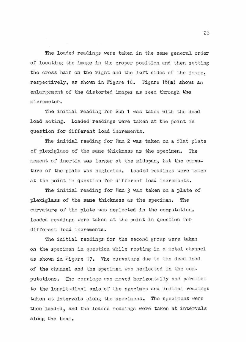
The loaded readings ·v1ere taken in the same general order
of locating the image in the proper position and then setting
the cross hair on the right and the left sides of the imc.ce,
respectively, as shown in Figm'e 16. Figure 16(a) shows an
enlargement of the distorted images as seen through the
micrometer.
The initial reading for Run 1 ·vms taken ·~:~i th the dead
load acting. Loaded readings \•Tere tal~en at the point in
question for different load increments.
The initial reading for Bun 2 was taken on a flat plate
of plexiglass of the same t hickness as the specimen. The
moment of inertia \vas larger at the midspan, lx1.t the curva
ture of the plate vras neglected. Loaded readint;s '.·rere ta1:en
at the point in question for different load incrernonts.
The initial reading for Hun 3 vias taken on a plate of
plexiglass of the same thickness a s the specimen. The
curvature of the plate \vas neglected in the computation.
Loaded readings \·Tere ta1ren at the point in question for
different load increments.
The initial readings for the second group \vere tal:en
on the specimen in questj_on vrhile resting in a metal chc: .. nnel
as sho~1 in Figure 17. The curvatur e due to the dead load
of the channel and the specimex~ v.rn. s negl ected in the con-
putations. The carriage Has moved hori.zontally and parallel
to the longi t u.dinal axis of the specimen and initial rea1..iings
taken at intervals along the specimens. The s pe c imens \-!ere
then loaded, and the loaded readings vrere taken at intervals
along the beam.
Page 41
29
F1 ur 11t-. I:m.strum .n·t'at"16n ;or runs 1, 2 and 3
Page 42
30
F1 ur 15. I tr t ti
Page 43
Outside ~'---...... _
ring
Inner core--
A
A
(3}
Zero curvature
Concave, curvature
2)
Convex curvature
(1) Centering position
(2.) Neasuring right side
(3) Measuring lei't s:tda
Figure 16. Image measurement
31
Page 44
~~~ \
•'
Image formed by . dead load curvature
tii!aa~ . ro;rmed by >:, c~~~x durvat~e
:1 ,,,
Image formed by . con:c·ave curvature
Figure 16(a). Distorted images
Page 45
Figur 1?.
f
Channel support for zero readings for runs 4, ; and 6
33
Page 46
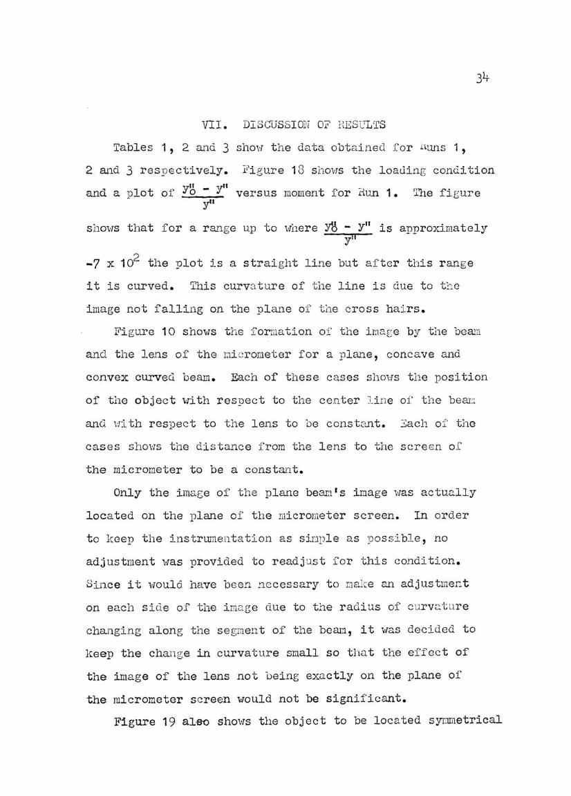
VII. DISCUSSION 01? RESULTS
Tables 1 , 2 at'ld 3 shoi1 the data obtained for HLms 1,
2 and 3 respectively. :i?igure 18 sho1,rs the loading condition
Yn _ ..,rtl and a plot of o J versus moment for Hun 1. 1'he figure
yl'
shol<'lS that for a ra..11.ge up to vThere t6 Y11 is approximately yfi
-7 x 10² the plot is a straight line but after this range
it is curved. 1'his curvature of the line is due to the
image not falling on the plane of tJ:1e cross hairs.
Figure 10 shm.vs the forn1a tion of the ir:1af:e by tl1e beam
and the lens of the mi·:~rometer for a plc,..'1e, concave and
convex curved beam. Each of these cases shm·rs the position
of the object vrith respect to the ce.nter :Line of the bee.Ll
and 1rL th respect to the lens to 'be const<:-.nt. 3ach o:f' the
cases shm·IS the distance from the lens to the screen of
the micrometer to be a const.::l.nt.
Only the imae;e of the pl<:me bear.'l 1 s image 1vas actually
located on the plane oi' the micrometer screen. In order
to keep the j_nstrLU}lentation as sinple as pos~:ible, no
adjustment \..ras provided to readjust for this condi tj_on.
Since it vrould have been necessary to oal:;:e an adjustmer:t
on each side of the imc~ge due to the radius of curv<.;,ture
changing along the segm.ent of the beam, it \vas decided to
lceep the change in curvature small so that the effect of
the image of the lens not being exactly on the plane of
the micrometer screen vrould not be significant.
Figure 19 aloo shm·rs the object to be located synmetrical
Page 47
35
vri th the center line of the lens. For Huns 1 through 6 the
object \vas located slightly off center to allovr the lens to
function. The amount of the object being off center vras
very small vlhen compared with the object distance of the
lens and 1-1as neglected in this study.
Figure 18 gives a larger ~ - Y'' value for a moment yt• -
than would be expected if the straight line portion is
extended. This difference agrees \•li th the case for conc :_.ve
curvature as shown by Figure 19.
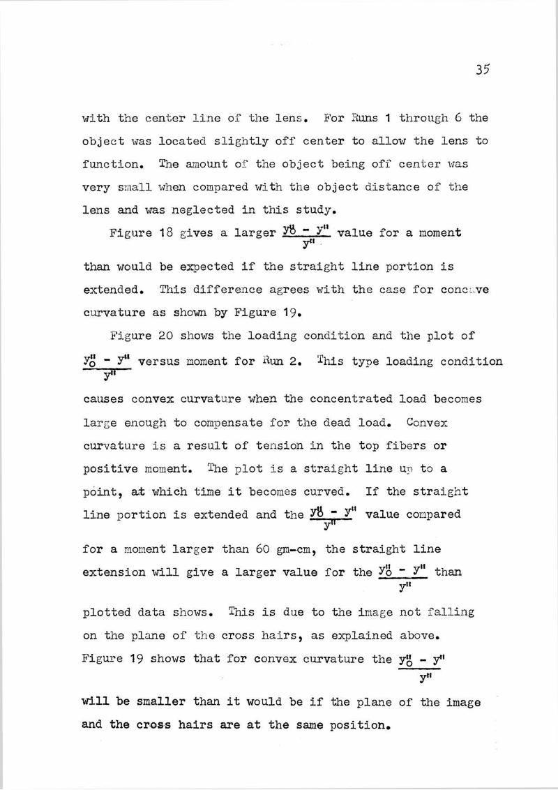
Figure 20 shows the loading condition and the plot of
yg - 7' versus moment for Run 2. This type loading condition yh
causes convex curvature when the concentrated load becomes
large enough to compensate for the dead load. Convex
curvature is a result of tension in the top fibers or
positive moment. The plot is a straight line u~' to a
point, at "IIThich time it becomes curved. If the straight
line portion is extended and the YB - Y" value compared yfl
for a moment larger than 60 gm-cm, the straight line
t · ·11 · 1 1 _.oor the Y'o' - Y" than ex enslon Wl glve a arger va ue , y"
plotted data shm-1s. This is due to the image not falling
on the plane of the cross hairs, as explained above.
Figure 19 shO\vS that for convex curvature the yg - y' ytt
will be smaller than it would be if the plane of the image
and the cr~ss hairs are at the same position.
Page 48
Figure 21 shovlS the loading c ondition a..lJ.d the -plot of
You - .,.u t "' ~ · 3 .Y versus momen i or ..:•un • The plot of Y3 - Y"
:t'
versus moment plotted a straight line in this ca se since
36
the curvature of the specimen ·vias small enough to elimina te
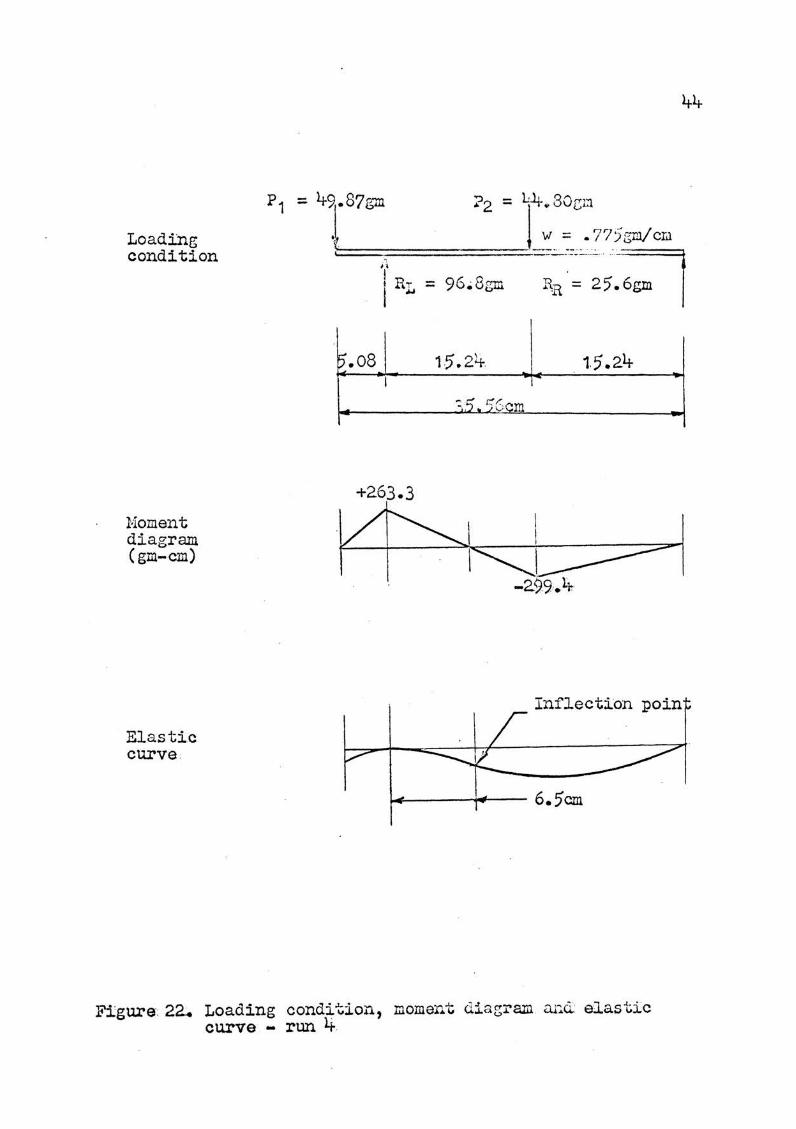
the image being out of focus.
The loading conditions, moment diagrams and elastic
curves are shovrn in Figures 22, 23 and 24 for 1-\uns lt, 5 and
6, respectively.
Table 4 shmvs the initial readings for Huns 4, 5 and
6. Table 5 shows the loaded readings for Runs 4, 5 and 6.
Figures 25, 27 and 28 shows a plot of the initial
readings (yg) and the loaded readings (y") versus distc:~nce
for nuns 4, 5 and 6, respectively.
Tables 6, 7 and 8 shovJ yg - yn , y'' and the experinen tal
moment computed from Eq. 20 for Runs 4, 5 and 6, respectively.
Figure 26 sho"'.vs a plot of the experinental monent and
the theoretical moment f or .i:iun 4. It can be seen that the
curves a cree Vli thin experimental accuracy along the full
length of the s pecimen.
F'igure 29 shovTS a plot of the experimen tal and the
theoretical moment s vers :J.s distru-1ce for itt..m 5. The moments
agree \d thin experir1ental accuracy along the length of the
beams.
Figure 30 sho•ds a plot of the experimental and the
theoretical moments versus distance for Hun 6 . The theo-
retical moment is seen to be considerably larger for the
Page 49
37
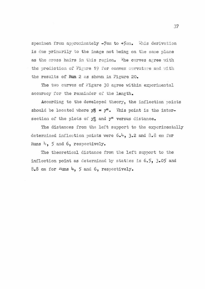
specimen frora appro:;.:ir:1a tely -7cm to +5en. j_'his derivation
is due prin:::.rily to the inage not being on t h e scuJe plane
as the :::Tos s hairs in this region. '.J..'he curves acree 1'l'i th
the ·:·n·ed ·ictio:l o-r Fi ~,·~ rr·e 10 ·ror convex :··q rva•- ,, ,,e and ,.,..: t h • --~ _., .}_ - (~; '- ·- / ..;,., ... ._, 'v ·• • V '-'•• •• ,.1 • . ~ j _ •
the results of Run 2 ;:,:.s shmm in Figure 20.
1,he t vJO curves of l."igure 30 a gree \-Ti thin expcriuental
accuracy for the re:·nainder of the length •
.According to the developed theory, the inflection -ooints
should be located 1;lhere y8 ; yn. This point is the inter-
section of the plots of y~ a..rJ.d y 11 versus distance.
The distances from ths left support to the experimentally
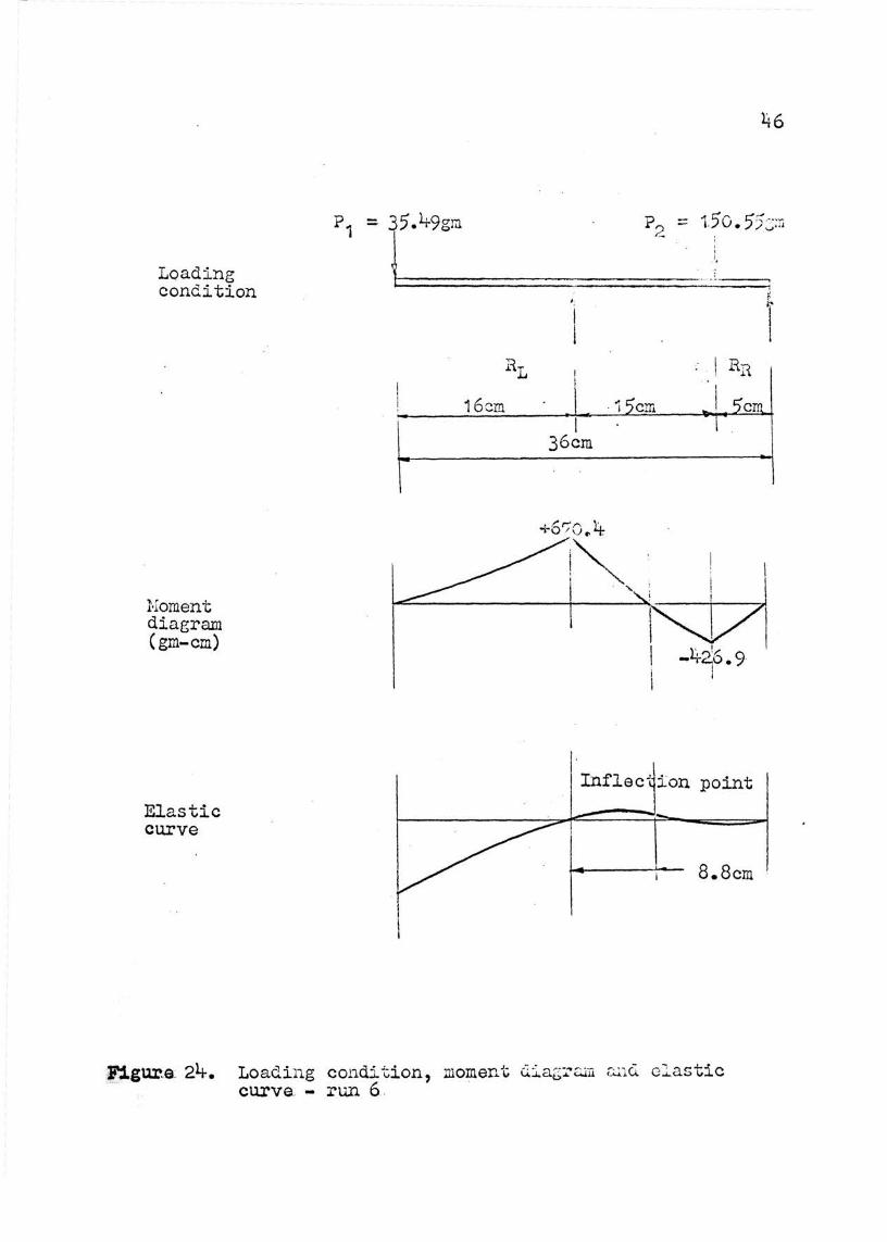
determined inflectj_on points \vere 6.4, 3.2 and 3. 8 em for
Runs 4, 5 and 6, respectively.
The theoretic2.l distanc e from the left suppol..,t to the
inflection point as determined by stat:l.cs is 6.5, 3.05 and
8.8 em for .J:\uns 4, 5 and 6, respectively.
Page 50
TABLE I.
Loaded Readings
Load Noment Y" (gm) (gm-cm) (Div)
11-.2 -12.7
8.4 -25.6
12.6 -38 •. 4
16 •. 8 -51 •. 4
21.0 -64.0
* Y" = -11 2. 5 Di v 0
-115.0
-117 • .o
-119.0
-121.0
-127.0
TABLE II.
- B.tm 1
y" - )''* ~Div
+ .2.5
+ 4.5
+ 6.5
+ 8.5
+14.5
Loaded Readings - Run 2
Load (gm)
Dead Load
4.2
8.2
12.6
16.8
20.7
24.9
29.1
1:-loment (gm-cm)
- 25.6
~.3
+ 11.0
+ 38.4
+ 59.6
+105.0
+126.8
+148.0
** y" = -101.1 Div 0
yu (Div)
-101.5
- -100.1
- 99.6
- 97.2
- 96.2
95.5
- 95.3
- 95.5
y'' - Y" ** ~Div)
+0.4
-1.0
-1.5
-3.9
-4.9
-5.6
-5.8
-5.6
38
Y8 II 2 - y X ·10 yu
- 2.2
-- 3.8
- 5.5
- 7.0
-11.4
Y3 - yu 2 __.;;... __ X 10 yn
-0.4
+1.0
+1.5
+l.J-.o
+6.1
+5 0 . /
Page 51
TABLE III.
Loaded Headings
Load Homent (gm)
8.4
16.8
25 .• 2
64.3
80.8
97.3
127.8
144.3
160.8
190.8
207.3
223.8
*Y11 = -101.7 0
(gm-cm)
- 30.7
- 61.5
- 91.9
-233.5
-294.5
-355.5
-465.0
-526.0
-?86.0
-695.0
-756.0
-815.0
Y'' (Div)
-102.4
-102.6
-102.5
-104.0
-1o4.1
-104.3
-105.8
-105.8
-106.4
-107.3
-107.5
-108.5
39
- ltWl 3
~· - yu* Yt] · - Y"x 10 2
~Div) yil
+0.7 -0.7
+0.9 -0.9
+0.8 -0.8
+2:.3 -2.2
+2.4 -2.3
+2.6 -2.5
+4 •. 1 -3.9
+4.1 -3.9
+4.7 -4.4
+5.6 -5.2
+5.8 -5.4
+6.8 -6.3
Page 52
4o
Y"-Y" 0 x102
y t I
-10
-15 ~--------'-------'1----...J -100 -50 -25 0
Moment (gm-cm)
Figure . 18. ~1x1o2 versu~ moment - run 1
Page 53
B
0~11 \ A '\
I I
\ \
I I \
: \
A'
I I
. I ,.
Pl a;:-~c of cross hairs
Lens Object
1.·
I I
---~~~~-~t-\~1-+~ Longitudinal 1 ! \ I axis of bean;. I I
:I \ I II ~ I
I I II I I \ II II
I I ~ 1 ~: \ II L __ j I ,I \
L I _j
Convex image
Flat image
Concave image
L -- ~ L --
Figure 19. Location of the images formeci by -..;:ne l t;..:lS for flat, concave and convex beams
~- 1
Page 54
n . ....u 2 Y 0 ":' -1 x1 0 · . yu
+8
+6
+2-
'0
-2 -50-·
42
5.08 ·I r 12.24~ 1 A. f-t-5.08 ' 1 I
7.88 i ; 8 :-- ·-11.1 I em
...
v ~
,j .
..
v. I
I · 0 1;50 175
Moment ~gm-cm)
ent - run Z
Page 55
yn-yu 0 :x:102 . yn
p
A.-- t
0~------~------~--------~------~----
-8--------._------~------~~------~--~ -900 · -700 -$00 -300 -100 0
· Homent (gm-cm)
li'igura a.t. Y&-Y11 .JC1o2 VGrsus moment . - run 3 :y" .
Page 56
Loading condition
Noment diagram (gm-cm)
Elasti.c curve
P1 = 49r87gm
~~
~.08 ..L
15.24
Inflection poin
~--__......,~- 6.5cm
Figure 22.4 Loading condition, moment di as;ram ar.cl eJ.astic curve - run 4
44
Page 57
Loading condition
Homent diagram (gm-cm)
Elastic curve
P1 = lr9.87gm
-775gmlcm
p2 = j 3lt. 09 gr.:
l ~ ~:
Inflection iPoint
Figure ~3'• . Loading condition' 'momQnt· OJ.agram d l tic curve - run 5 ·· · ··· ~ ·· . ·
45'
Page 58
46
p1 p 2
:::: 150 5~---:-• • /,_,. .. J
Loading ····· ·-
"' r·49gm
condition -·
t
Noment diagram (gm-cm)
Elastic curve
f:igur.a: 24.
•
l RL I I Rn
I
16cm I ·15cm I 5cm I I
36cm
Inflec~ion point
8.8cm
Loading condition, moment uia6~~n wlQ clastic curve. - run 6
Page 59
47
TA1JLE IV.
Initial Readings - Runs 4, 5 and 6
Run Distance Y8 (em) ( Oiv)
4 - 2.5 -105-7
4 6.0 -106.0
4 12.0 -105.0
4 15.5 -105.0
4 22.0 -105.2
4 31.0 - ~106.0
5 - 2.5 -106.3
5 6.0 -106.8
5 12.0 -106.0
5 115-5 -106.0
5 22.0 -106.0
5 31.0 -106.0
6 -15.0 -117.2
6 -10.0 -117.0
6 - 5·0 -116.9
6 0.0 -116.0
6 5.0 -116.0
6 10.0 -116.3
6 15.0 -116.3
6 19.0 -116.3
6 20.0 -117·5
Page 60
48
TABLE V.
Loaded Readings Runs 4 .-' and 6 - ' :..>
Hun 4 Hun 5 RLm 6
Distance Y" Distance y" Distance ~rll
(em) (Div) (em) (Div) (em) (Div)
-4.6 -105.0 _LI-. 7 -107.1 -15.0 -116.2
o.o -103.5 -2.0 -105.5 . -12.5 -115.7
2.0 -104.6 o.o -104.6 -10.0 -111.1 .• 8
4.0 -105.4 2.0 -105.5 - 7.5 -11Y-.O
6.0 -105.8 4.0 -107.0 - 5.0 -113.8
8.0 -105. 9 6.0 -109.2 - 2.5 -113.0
10.0 -106.7 8.0 -111.3 o.o -112.5.
12.0 -107.5 10.0 -112.3 2.5 -113.2
1 L1-.0 -107.5 12.0 -11 1~· .3 5.0 -113.9
16.0 -10'7.9 1 Lr. 0 -117.5 '7. 5 -115.5
18.0 -107.2 16.0 -116.2 10.0 -116.11-
20.0 -107.4 18.0 -114.2 10.5 -116.7
22.0 -106.6 20.0 -112. 8 12.5 -117.7
2lt.O -107.1 22.0 -110.6 14.0 -119.1
26.0 -106.1 21.1-.0 -109.8 15.0 -11 9.6
28.0 -106.6 26.0 -108.6 17.5 -118.1
30.0 -106.2 28.0 -107.3 19.0 -117.2
30.0 -105.5
Page 61
-100
-102
Y" (Div) 6 -10
+ •
..,.,
?
Yo" yn ·
-->./1\ v · ~ ~
' -~ I ! I !
l
l
-'- -L ~
fo"" -~ ----- ...._ T
-108
~ ~
~ L?v. ~
~ .. , .
- 110-10 -5 0 5 10 15 20 25 . 30 35
Distance ( CJ:!l)~
Figure 25. Initial and loaded readings vers~s distance - run 4
Mo (gm-cm) :
600
4oo
200
· o
-200
• • • ExperimentaL ---- Theoretical
j \. v ·~ r\.. ~
~ ~ ./
v ~ v-r-"
. -4<>~10 -5 0 5 10 1$ 20 25 30 35
Distance (em) · .. ~
. Figiire 26 •. Experimental and· theoretical mo:4ent_s ...........,,,..., distance - run lt · ·~
Page 62
-96
-100
-104
... yu -108 (Div}
-112
-116
-120
• +
Y'' yt6
I ~ 7
. •
.
"- ' "<; r- •
"'· ~ y
~
~ I
I I l i ---- . ---
I· I I
\ I - ··· -- ---·
_!. _!_ ~ • L :+
L!_ v
L v
II"
-10 -5 0 5 10 15 20 2.5 30 35
· Figura 27.
-110
-112
-114
yll -116 (Div)
-118
-12.0
-124
Distanca (em):
Initial and loaded readings versus ciista:..1ca - run 5
• yll
+ n Yo
L / "t /
v -~ . :,
\ 3.. ' .-1---t v ~ 'l\ !.
,/ -L~
..
\ vI ' I -
-20 -15 -10 -5 0 5 10 1:5 20 25
Distance (c:n)
Figure 28. _ Initial and loaded raadL~gs versus distance -run 6
50
Page 63
51
TABLE VI.
Experimental Homent - Hun 4
Distance y" - )11 t' Y8 - Y" 2
Experimental (em) ~Div X 10 ( DJ. v) y" Noment
(gm-cm)
-5.08 o.o -105.2 o.o 0
-2.50 -1.3 -104.4 +1.25 +148
-0.00 -2.5 -103.5 +2.42 +286
2.50 -1.4 -104.8 +1.33 +158
5.00 -0.5 -105.6 +0.47 + 56
7.50 +0.4 -106.2 -0.39 - 45
10.00 +1.4 -106.8 -1.31 -155
15.00 +2.6 -107.8 -2.41 -286
20.00 +2.1 -107.3 -1.95 -232
25.00 +1.2 -106.6 -1.13 -133
30.00 +0.1 -106.0 -0.09 - 11
30.50 o.o -105.9 o.o 0
Page 64
52
TABLE VII.
:E...':cperi:me:1tal Loment - Hun 5
Distance y" - rl tl Y" - yn 2 Experimental 0 X 10 (em) ~Div (D~v) yt1 Hor1ent
(gm-cm)
- 5.08 o.o -107.2 o.o 0
- 2. 50 - 0.8 -106.1 +0.75 + 89
o.oo - 2.1 -104.6 +2.01 + 238
2.50 - 0.7 -106.0 +0.66 + 78
5.00 + 1.7 -108.0 -1.57 - 186
7.50 + 4.9 -111.1 -4.41 - 523
,10.00 + 6.2 -112.3 -5.50 - 651
12.50 + 8.8 -114.8 -7.66 - 910
15.00 +10.7 -116.7 - 9.18 -1088
20.00 + 6.5 -112.5 -5.78 - 685
25.00 + 3.1 -109.1 -2.84 - 336
27.50 + 1. 5 -107.5 -1.34 - 166
30.50 o.o -106.0 o.o 0
Page 65
53
TABLE VIII.
Experimental l·ioraent - Run 6
Dista11ce vu - y" yll yg Y'' 2 Experimental - X 10 (em) "~Div) (Div) II l·ior.1ent y .
(grJ-cm)
-16.0 o.o -117.2 o.o o.o -15.0 -0.5 -116.7 +O.Y-3 -1 52.4
-1 0.0 -2.1 -11 4. 9 +1.83 +223.0
- 5.0 -3.3 -113.6 +2.91 +354.0
o.o -3.5 -112.5 +3.13 +381.0
5.0 -2.0 -113.9 +1.76 +214.0
10.0 +0.8 -116.6 -0. 69 - 84.0
12.5 +2.2 -118.0 -1.86 -227.0
15.0 +4.1 -119.8 -3.42 _tl-16.0
.17. 5 +2.l.t -118.1 -2.03 -2LJ-7 .0
20.0 o.o -116.5 o.o o.o
Page 66
+800
+600
+200
l.fo (gm-cm) . 0
-200..-
-ltoo
-600
-800
-1000
-1200
• • • EA~erimental
---- Theoretical
~ v \ I
\ I
I I i
I
I I i
I i
1
:
I -10 -5 0 5 10 20 30
Figure. 29...
Distance (em)
EA~erimental and theoreti cal momonts VGTs~s distance - run 5
54
35
Page 67
1.200
1050
Experimental ! I
' •••
----- Theoretical I I I
900
. 750
600
·+::·1J.5o
/ \ I
~ .
\ I \ I
\
300
1150
Mo 0 (gm-cm)
-150
-300
I ~ !'\.\ l
/~ ,,
/ v. ,\ \ .
1\, I \ I
\ I .. ,, \ I \ w
-450
-6~20 -15 -10 -5 0 5 10 1:5 20 25
Figure~ 30.
Distance (em)
Experimental and theoretical moments V6J:'SUS distance-~ 6 .
55
Page 68
VIII. CONCIXSIONS
From this study, the f'ollmiing conclusions l.va.ve been
made.
1. The mornent in a beam is directly proport ional to
Y0" - Y11 when EI is a constant.
y"
2. The inflection points can be located by the use
of the optical relationships developed •
. 3. The moment diagram for a berun can be plotted by
the use of the derived optical relationship.
4. To allov7 great er precision in the measuring a.'1d
greater curvature to be :measured, the lens should have
greater magnification and an internal focusing device should
be used to eliminate the parallax caused by the inage plane
not coinciding "~•Ji th the plane of the cross hairs.
5. To allow the data to be repea ted more readily, an
object that remains a. constant size •.-.rhen the licht source
is replaced should be provided.
6. To facilitate the measuring, the brightness of t he
object should be increased.
Page 69
57
IX. RECOHhEI'JDATIONS
As a result of the investigation of this thesis, certain
recorrunenda tions follo\IT:
1. The theory should be e:A."":panded to include curved
beams and arches; and tests made to demonstrate its appli
cation.
2. The theory should be expanded to include plates
and shells. In these applications, the size of the image
should change along both axes since the moment along both
axes wilJ be changing.
3. The study should be expanded to include indeter
minate beams, beams of variable moment of inertia, and
frames.
4. A study should be made to demonstrate the :;;easurment
of rotation of a segment of a structure similar to the method
of measuring the slope of a membrane analogy as noted in
the Review of Literature.
5. To eliminate the effects of' creep and permanent
distortions, other materials should be tested. One might
try a netal bea..'ll that has either a polished surface, or
segments of its surface polished.
Page 70
APPEHDIX I
The graphiS!al procedure used to shmv the formation of
the image by a curved rllirror shown in :Figures 5 and 6 is
explained as folloHs (3):
58
1. A ray parallel to the axis. After reflection,
this ray passes through the to cal point of a
concave nirror or appears to come f rom the
focal point of a convex: mirror.
2. A ray from (or proceeding to~rard) the focal
point. This ray is reflected parallel to the
axis
3. A ray along the radius (extended if necessary).
'rhis ray intersects the surface normally and
is reflected back along its original path.
The graphical procedure used to show the formation o:f
the i mage by a thin lens of Figure 8 is explained as
follm·rs (3):
1. A ray parallel to the axis. After ref raction
by the lens, t his ray passes througll the second
focal point of a converging lens, or appears
to come froM the second focal point of a di-
verginr; lens.
') '-• A ray througi1 tile center of tJ.1e l ens. This
ray is not apprecL~.bly devi,:..tted, s :i.nce the hw
lens surfaces through \•Thich the centre .. l ray
passes are very nearly parallel i f the l ens
is thin. A ray passing through a plate \fl th
Page 71
parallel faces is not dev:Lated, but only
displaced. .1.'or a thin lens, the displacenent
may be neglec t ed.
59
3. A ray through (or proceeding toward) the f irst
focal point. This ray emerges parallel to the
axis.
Page 72
APPKWIX II
The product of EI for the specimen used in Runs 4, 5
and 6 was determined by the use of a cantilevered segment
of t he beam 1vi th a concentrc.l. ted load on its free end.
The general equation used ,,.;as as follovTs:
PL3 ~· = 3EI
where
s = p = E = I =
Deflection,
Load,
Nodulus of elasticity, and
}foment of inertia.
60
·vJhen a plot of deflection versus load is made, the slope
of t he line is eq ual to 13 • Thus, EI can be computed by 3EI
measuring the slope.
Figure 31 shows the general test equipment used to
measure EI. The beam t>Tas clam·:·!ed bet\•leen tvTO alw-11inwn angles
to give a fixed-end condition. A needle was attached perpen
dicular to the end of the beaY.l , a scale was positioned at
the end of t he needle, and the concen·Gra ted loads \:ere placed.
in the pan.
A specimen t aken from t he same sheet of plc:x:iglass as
t he s peci rJen used in Runs 1.:. , 5 and 6 \vas checl~ed f or cr eeD
under a constan t load. The specimen ,,ra s .1.1 11 ':.ride and nominal
1./411 thick. The loading condition is shown in Figure 32.
The zero reading ·Has taken -vri th the loading pail on the beam.
A 100 gm weight was placed in the pan and readin:;::s ta~:en a s
shm·m in Table 9.
Page 73
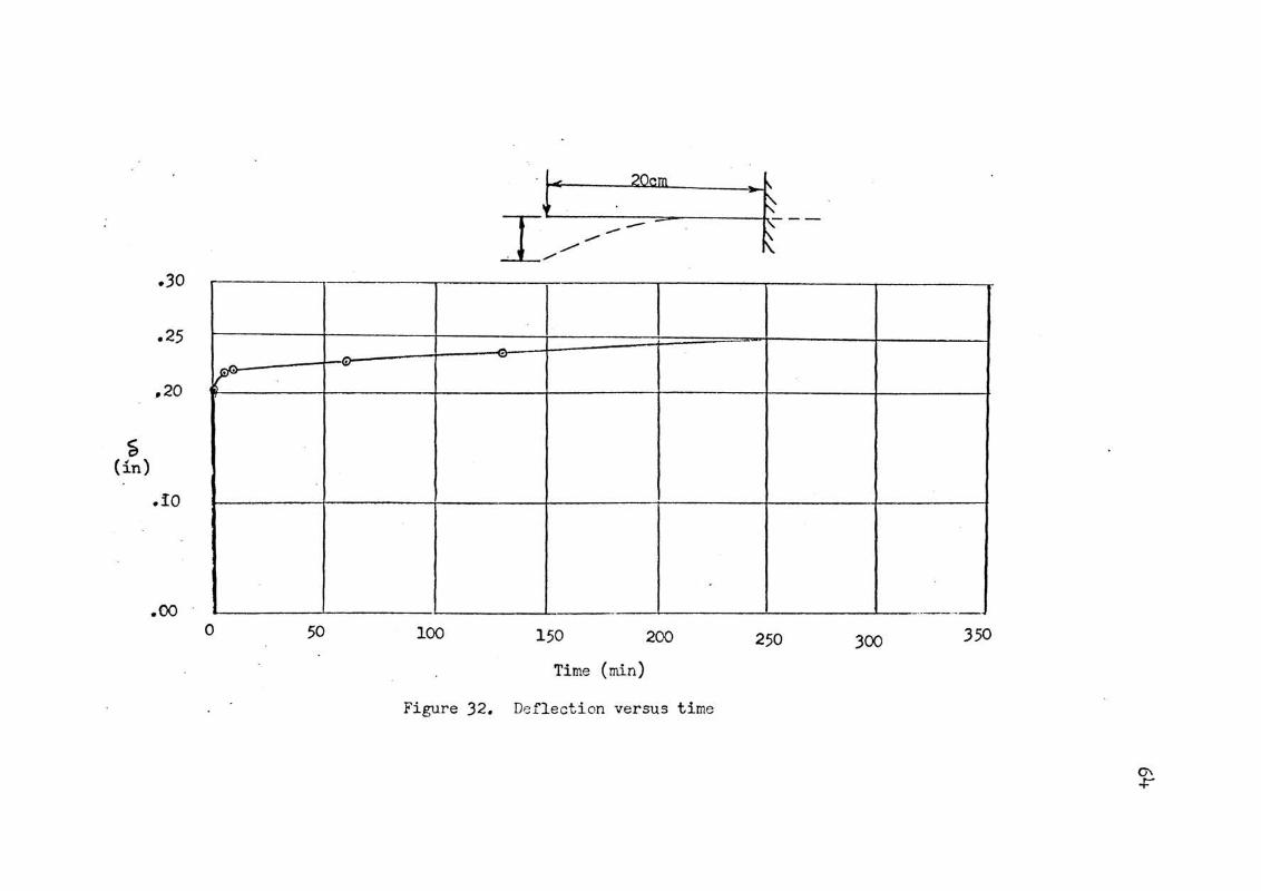
Figw:·e 32 sho\vs a plot of deflection versus time, a.:nd
that the major portion of the creep deflection tal;:es place
in a reasonably short period of tina.
61
To alloH for the effect of the creep o:f the plexiglas.s,
the readings for the runs on the specimen for Runs 4,5 and 6
were taken to minutes after the increment of load had been
placed in the loading pan.
Three sets of data ".vere taken for the speci~:1en. The
three loading conditions are shown in Figure 33 as Case 1, 2
and 3, respectively. The data for the three cases are shmm
in Table 10.
The plots of deflection versus load for Cases 1, 2 and
the average of t and 2 are shmvn in Figure 34-. The respective
EI's ar ':: 5.02 x 10⁵, 4.86 x 10⁵ and 4.93 ?\: 105 gm-cm2 •
The plo.t of deflection versus load for Case 3 is shown
in Figura 35. The EI was computed from the slope to be
lt. 95 x 105 gm-cm2.
This EI compe.red '\'li thin the limits of experimental accu-·
racy to the average of Case 1 and 2, and ·vias used for the
specimen.
Page 74
62
Figur 31. cantilevered beam
Page 75
63
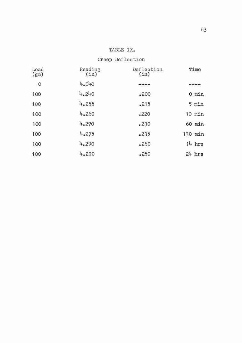
TABLE IX.
Creep Def lec tion
Load Reading Def lection Time (gm) (in) (in)
0 lt-.04o
100 4.240 .200 0 min
100 4.255 .215 5 min
100 4.260 • .220 10 min
100 4.270 .230 60 min
100 4.275 .235 130 min
100 4.290 .250 14 hrs
100 4.290 .250 2l.r- hrs
Page 76
.oo 0 50
I~ . 20:: ~~ --
' --------100 150 200 250 300 350
Time (min)
Figure 32. Deflection versus time
0\ +
Page 77
65
Case 1
p
17.9cm '>I
r===-==---
Case 2
p
- :::::: - ~·.·-\ -- . j
-- <::" -- c - ..... J.
Figure 33. Loading conditions- cases 1, 2 ru1d 3
Page 78
66
'J~ABLE X.
Deflectio=l of Cantilever Dearils
Case 1 Case 2 Case 3
Load .., Load ..., Load (gm) (inx10.)) (gu ) (inx10.)) ( gm) ( r::u:; )
0 0 0
10 15 10 15 5 0.7
20 35 20 30 10 1.5
lto 65 ~-o 60 15 2.5
60 95 60 90 20 3.5
70 110 80 120 25 lt-.5
110 1 '70 110 16 5
11t0 220 1ltO 210
Page 79
67
24o -i • • Case 1
I I I ...., __ .._ Case 2 Average I
! --- i !
200 1
1.60
120
80
4a
Q; 0 40 80 120 160
P (Load in gm.)
Figure 34. Deflection varsus load- cas es 1, 2 and. average
Page 80
68
4.0
3.0
s {mm) ' 2.0 ~------~~----~------~
1.0
o.o 0 10 20 30
P (Load in gm)
Figure 35. Deflection versus load - case 3
Page 81
69
DIDLIOGHAPHY
1. LEE, GEORGE HALOR,(1963). An Introduction to Experine.ntal
Stress Analysis, 6th ecl.i tion John ~'Iiley
and Son, Inc.
2. EURPHY, GLENI'-r , ( 1950). Similitude in En.&~ineering 'I'he c .. - '
Ronald Press Company.
and ZE1·iAJ:SEY, H. \1., ( 19 55). University
Physics, 2nd edition Addison-Wesley
Publishing COE1pany, Inc.
4. \'lANG, CIEJo-KIA, and ECKEL, CLAHEIJ CE LEvHS,(1 9 57).
Elementary Theory of Structures, J.icGrav.r
Hill Boo.k Publishing Company, Inc.
Page 82
70
VITA
Jitlrny Dean Hahs, the son of Raymond and Till ere (Statler)
Hahs, vras born on Har.ch 13 , 1.91+0 at Sedgewickville, l<issouri.
He attended the·. Cape Girardeau, l-lissouri and t he
Farmington, Hissouri grade schools and the Farmington,
Hissouri high school, from which he graduated in 1957.
He attended Flat River Junior Colleg-e in Flat River,
Hissouri for one year and in 1958 he enrolled at the Hissouri
School of ~'fines: and Hetallurgy and r .ecei ved the degree of
Bachelor of Science in Civil Engineering in Nay, 1961 from
that institution. He also attended Tulsa University,
Tusla, Olclahoma, Joliet Jnnior College, Joliet, Illinois,
and Northern Illinois University, DeKalb, Illinois.
His professional experience has CO !~Sisted of employment
with Texaco Incorporated, Illinois Highway Department, a:n.d
HcDonnell Aircraft Corporation. He received an assistantshi:;:~
to the University of Hissouri School of Nines and l-:Ietallurgy
in 1963, and \•ras appointed an Instructor in Civil Engineering
in 1964 vlhile working tm'lards the degree of Nastor of
Science in Civil Engineering .
In September, 1961 he vTaS married to Hiss Ruth Fope
of i:-ledora, Illinois. They have two children, Daniel and
Janet.