Copyright 2002, Marie-Pierre G. Laborie INVESTIGATION OF THE WOOD/ PHENOL-FORMALDEHYDE ADHESIVE INTERPHASE MORPHOLOGY By Marie-Pierre G. Laborie A Dissertation Submitted to the Faculty of Virginia Polytechnic Institute and State University in partial fulfillment of the requirements for the degree of DOCTOR OF PHILOSOPHY in Wood Science and Forest Products Approved by: Charles E. Frazier, Chairman Wolfgang G. Glasser Frederick A. Kamke Eva Marand Thomas C. Ward Alan Esker February 1, 2002 Blacksburg, Virginia Keywords: Wood /Adhesive Interphase, Glass transition, Cooperativity Analysis, Solid -State NMR
Transcript
Copyright 2002, Marie-Pierre G. Laborie
INVESTIGATION OF THE WOOD/ PHENOL-FORMALDEHYDE
ADHESIVE INTERPHASE MORPHOLOGY
By
Marie-Pierre G. Laborie
A Dissertation Submitted to the Faculty of Virginia Polytechnic Institute
and State University
in partial fulfillment of the requirements for the degree of
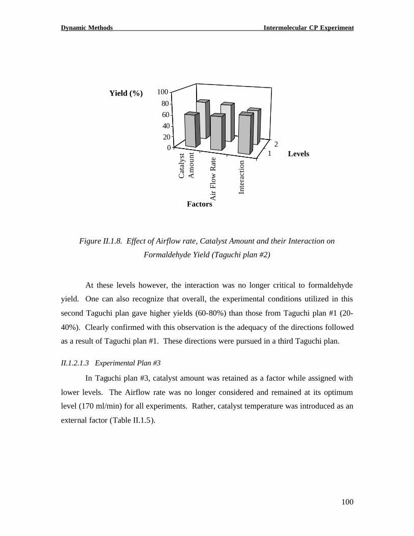
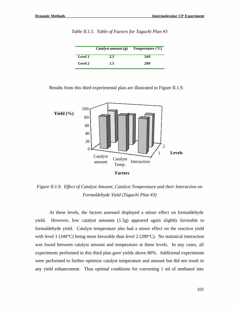
molecular motions are restricted by intermolecular coupling between non-bonded
segments. Hence, relaxation times in this temperature region are longer due to
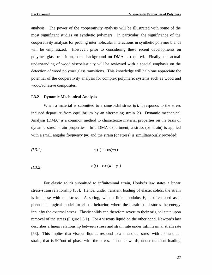
Background Viscoelastic Properties of Polymers
43
organization in cooperatively rearranging molecular entities. Matsuoka provides a
descriptive picture of the concept of intermolecular cooperativity among non-bonded
segments (Figure I.3.10) [58].
Figure I.3.10. Matsuoka Representation of Cooperative Domains with z=6 (from [58])
Again the occurrence of cooperative regions is nothing novel compared to the AG
theory. In the AG theory however, it is assumed that all cooperative regions z* (T) relax
simultaneously so that one single relaxation time describes the relaxation process at one
temperature (Equation (I.3.18)). This allows the AG theory to model the relaxation
process as a simple exponential function of time. It is empirically well established,
however, that the relaxation function near the glass transition deviates from simple
exponential behavior. In fact, for glass- forming polymers, the Kohlrausch-Williams-
Background Viscoelastic Properties of Polymers
44
Watts (KWW) equation describes a stretched decay function, φ(t), for portraying the
distribution of characteristic relaxation times (τ∗) around the glass transition [71]:
(I.3.30) ( )[ ]βτφ ∗−= tt exp)(
In Equation (I.3.30), β (0 <β ≤ 1) is the non-exponentiality parameter which
describes the distribution breadth of relaxation times [71]. Recognizing this major pitfall
of the AG theory, Ngai proposed to reconcile the AG approach with the experimental
observation of non-exponential behavior of the glass transition dispersion. Specifically,
Ngai argued that in condensed matter, interactions between neighboring molecules
impede simultaneous and independent relaxation of cooperative regions [72]. Rather,
intermolecular interactions generate dynamic heterogeneity, which is well portrayed by a
distribution of relaxation times. At a temperature- insensitive cross-over time tc,
molecular relaxation changes from an independent and exponential process to an
intermolecularly coupled process. At times below tc, the relaxation function is equivalent
to that obtained from the AG theory with independent and simultaneous relaxation:
(I.3.31) ( ))(exp)( Ttt τφ −=
For time scales longer than tc however, intermolecular interactions slow down the
relaxation process so that the relaxation function becomes a stretched exponential
function as in the KWW expression:
(I.3.32) ( )[ ]nTtt
−−=
1* )(exp)( τφ
In Equation (I.3.32), the coupling constant, n, quantifies the extent of
intermolecular coupling among non-bonded segments and assumes values from 0 to 1. It
is easily seen that the coupling parameter relates to the KWW exponent as n = 1-β .
Continuity of the relaxation function at t = tc, allowed Ngai to generalize the coupling
model for any time scale as:
(I.3.33) ( )[ ] ( )nnc TnT −∗ −= 1
1
0 )(1)( τωτ
Background Viscoelastic Properties of Polymers
45
In equation (I.3.33), ωc is the crossover frequency between independent segmental
relaxation and cooperative segmental relaxation. Hence when n equals 0 the coupling
model describes a single exponential relaxation function with a characteristic time τ0 as
for a simple Maxwell element. When the coupling constant assumes a positive value, the
model describes a non-exponential distribution of relaxation times. High values of the
coupling parameter indicate high degrees of intermolecular coupling or cooperativity.
The equivalence between the magnitude of intermolecular coup ling and the breadth of the
relaxation spectrum proposed by Ngai is intuitively satisfactory. Indeed, polymers are
best described by statistical factors, such as average molecular weights, average topology
and average stereochemistry. Statistical heterogeneity in polymers yields molecular
motions that are dynamically heterogeneous hence generating a broad distribution of
relaxation times. As a consequence segmental relaxation does differ throughout a bulk
polymer sample. The more intermolecular coupling, the more each polymer segment has
its relaxation mechanisms influenced by the neighboring segments and the broader the
distribution of relaxation mechanisms. Hence the coupling model succeeds in
quantifying the deviation from exponentiality observed in polymeric glass relaxation.
What also clearly emerges from the coupling model is that the temperature dependence of
τ0 is amplified in the dense phase by the power 1/(1-n) as a result of intermolecular
coupling. Because the coupling model captures the temperature dependence of a
characteristic relaxation time, Plazeck and Ngai reformulated the model with a shift
factor function [73]. Taking the ratio of relaxation times at a temperature T and at a
temperature Tg, they obtained:
(I.3.34) )()(
log)()(
log)1(log)1(0
0*
*
ggT T
TTT
nanττ
ττ
=−=−
Background Viscoelastic Properties of Polymers
46
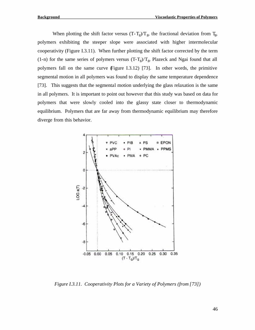
When plotting the shift factor versus (T-Tg)/Tg, the fractional deviation from Tg,
polymers exhibiting the steeper slope were associated with higher intermolecular
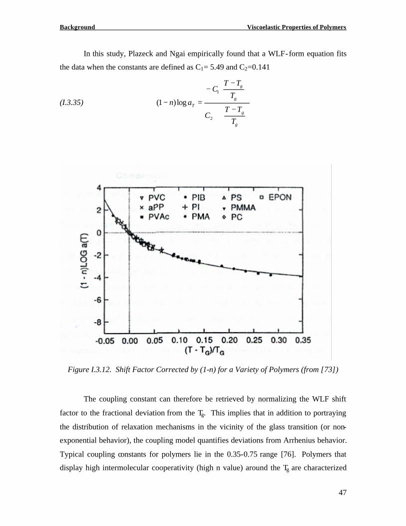
cooperativity (Figure I.3.11). When further plotting the shift factor corrected by the term
(1-n) for the same series of polymers versus (T-Tg)/Tg, Plazeck and Ngai found that all
polymers fall on the same curve (Figure I.3.12) [73]. In other words, the primitive
segmental motion in all polymers was found to display the same temperature dependence
[73]. This suggests that the segmental motion underlying the glass relaxation is the same
in all polymers. It is important to point out however that this study was based on data for
polymers that were slowly cooled into the glassy state closer to thermodynamic
equilibrium. Polymers that are far away from thermodynamic equilibrium may therefore
diverge from this behavior.
Figure I.3.11. Cooperativity Plots for a Variety of Polymers (from [73])
Background Viscoelastic Properties of Polymers
47
In this study, Plazeck and Ngai empirically found that a WLF-form equation fits
the data when the constants are defined as C1= 5.49 and C2=0.141
(I.3.35)
−+
−−
=−
g
g
g
g
T
TTT
C
T
TTC
an
2
1
log)1(
Figure I.3.12. Shift Factor Corrected by (1-n) for a Variety of Polymers (from [73])
The coupling constant can therefore be retrieved by normalizing the WLF shift
factor to the fractional deviation from the Tg. This implies that in addition to portraying
the distribution of relaxation mechanisms in the vicinity of the glass transition (or non-
exponential behavior), the coupling model quantifies deviations from Arrhenius behavior.
Typical coupling constants for polymers lie in the 0.35-0.75 range [76]. Polymers that
display high intermolecular cooperativity (high n value) around the Tg are characterized
Background Viscoelastic Properties of Polymers
48
by a broad distribution of relaxation mechanisms and a significant deviation from
Arrhenius behavior around the glass transition. On the other hand, polymers with little
intermolecular cooperativity (low n value) around the Tg are dynamically more
homogeneous and display a relatively narrow distribution of relaxation mechanisms as
well as near Arrhenius behavior. In this perspective, the coupling model has emerged as
a unique tool to further characterize polymer alpha transitions. The contribution of the
coupling model to the fundamental understanding of polymer viscoelasticity can be
appreciated by its remarkable success on a variety of polymers [74]-[78]. In fact,
intermolecular cooperativity has been explained on the basis of polymer chemical
structure [74]. As expected, structural features of the polymer backbone (polarity,
symmetry and steric hindrance) are reflected in the coupling constant [76]. In general,
polymers with smooth, flexible and symmetrical backbones display low coupling
constants while polymers with less flexible backbones, sterically-hindering pendant
groups and high polarity exhibit broader segmental relaxation and greater intermolecular
cooperativity [74]. For instance, Robertson and coworkers showed that the α relaxation
of polybutadienes broadens and intermolecular coupling increases as the vinyl content
increases from 1,4 polybutadiene to 1,2 polybutadiene [78]. Similarly, epoxydization of
1,4-polyisoprene promotes segmental cooperativity at the glass transition [75]. In fact,
the recent literature abounds with cooperativity studies on bulk polymers and the success
of the coupling model for investigating intermolecular interactions in bulk polymers is
well established.
Of greater interest for the scientist seeking to adapt such methods to
wood/adhesive composites are those studies that deal with polymer blends. A few studies
are available on polymer blends [79]-[84]. A review of cooperativity analysis for
common miscible polymer blends such as poly(vinylethylene)/ polyisoprene,
polyvinylmethylene/ polystyrene and tetramethyl polycarbonate/ polystyrene is provided
by Roland and Ngai [82]. Regardless of specific interactions in polymer blends, a
general trend indicates broadening and steeper temperature dependence of the alpha-
relaxation upon blending [82]. This phenomenon can be ascribed to the fluctuations in
local composition in the blend. In addition, Roland and Ngai often observe an
asymmetrical broadening on the low frequency side of the glass transition for miscible
Background Viscoelastic Properties of Polymers
49
polymer blends [82]. Inhomogeneous broadening is in accordance with the high Tg
component influencing the low frequency tail of the blend glass transition [82]. A more
recent study suggests that the cooperativity analysis may be utilized for probing specific
interactions in miscible polymer blends [84]. In this study, the temperature dependence
of relaxation mechanisms in blends of polystyrene (PS) and poly(2,6-dimethyl-1,4-
phenylene oxide) (PPO) is investigated as a measure of intermolecular cooperativity. It is
reported that PS/PPO blends display greater intermolecular cooperativity than that
expected on the basis of the neat polymers [84]. The authors point out that while
compositional heterogeneity in blends is generally invoked for greater cooperativity in
miscible polymer blends, attractive intermolecular interactions shall have a similar effect
on cooperativity [84]. It seems however difficult to assess the specific contributions of
concentration fluctuations and intermolecular interactions to enhanced cooperativity in
polymer blends. In this study nevertheless, both specific interactions and concentration
fluctuations are believed to induce the broadening and steeper temperature dependence of
the alpha-relaxation in PS/PPO blends [84]. More interesting, the coupling model has
been successfully applied to complex composite systems such as Epoxy/E-glass
composites [85]. For Epoxy/E-glass composites, the coupling constant afforded a more
sensitive probe of viscoelastic properties than the simple determination of glass transition
temperatures [85].
The widespread success of the coupling model for neat polymers and more
complex polymeric systems is well established. It is especially noteworthy that the
coupling model successfully describes relaxation in composites. Wood itself is a
complex composite structure of polymers. In spite of its complexity, one may expect that
the coupling model affords a greater understanding of wood viscoelastic properties. The
next section aims at reviewing the advances in the field of wood viscoelasticity.
Reviewing the actual knowledge on the viscoelastic characterization of wood will help
one appreciate the potential of the coupling model for wood itself but also for wood/
adhesive composites.
Background Viscoelastic Properties of Polymers
50
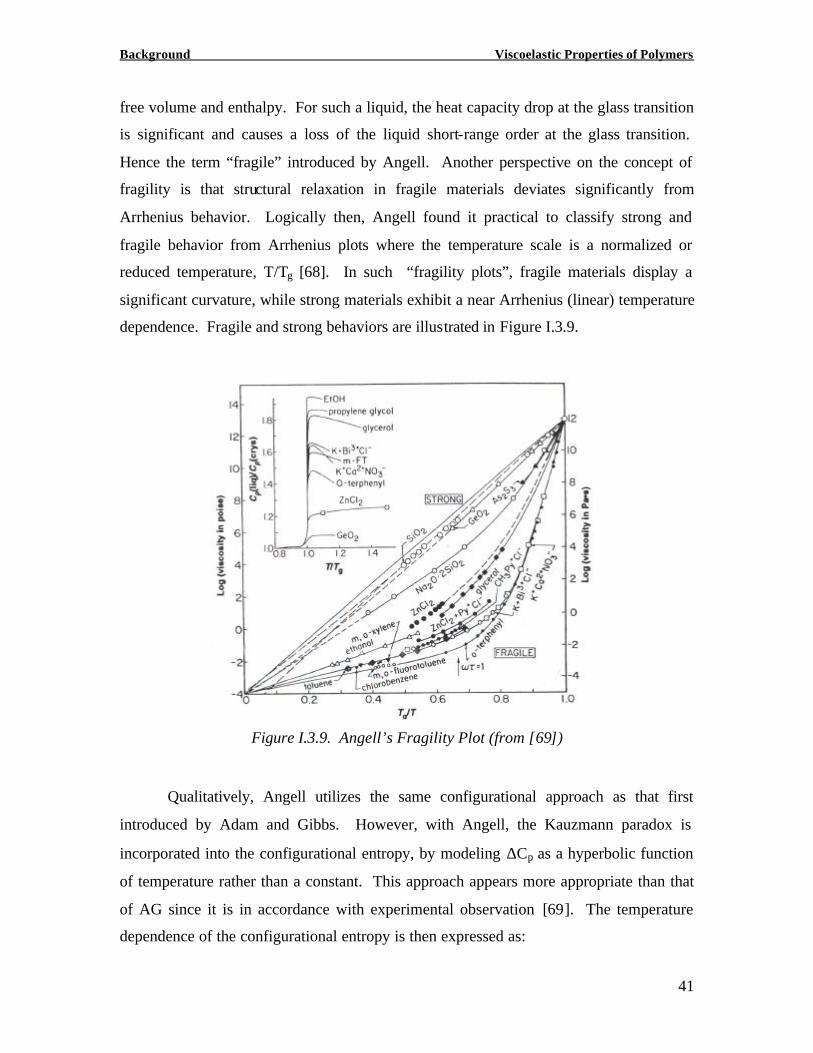
I.3.5 Viscoelastic Properties of Wood
Owing to its importance in forest product technologies, extensive efforts have
concentrated on wood viscoelasticity. Wood polymer glass transitions are particularly
critical to the manufacture of many wood products. For instance, lignin softening plays a
crucial role in pulp and paper manufacture [95]. As a consequence, the past two decades
have seen significant advances in the understanding and modeling of wood polymer glass
transitions. Along with these advances, analysis of wood viscoelastic properties has
emerged as a powerful tool to characterize the molecular scale changes induced by a
variety of treatments. Of particular interest for the wood adhesives field, changes in
wood viscoelastic properties may reveal wood/adhesive interactions [113]. In this
section, the reader is introduced to the most important advances in characterizing and
modeling wood viscoelastic properties. Analysis of wood viscoelastic properties as a tool
to probe interactions with extraneous compounds will also be discussed.
I.3.5.1 Viscoelastic properties of wood
Early studies have focused on the viscoelastic properties of isolated wood
polymers. While it is recognized that properties from isolated wood components may not
reflect the in-situ polymers, a thorough understanding of the viscoelastic response of each
wood component aids in comprehending wood viscoelastic behavior.
I.3.5.1.1 Viscoelastic Properties of Isolated Wood Polymers
Wood is a composite of 3 polymers, cellulose, hemicellulose and lignin. Each of
these polymers has a specific chemical structure, topology, molecular weight distribution
and morphology, and therefore they display different viscoelastic properties. Owing to
the importance of the cellulose industry, cellulose viscoelastic properties have been
extensively studied [86], [89]-[92]. Cellulose can be either amorphous or semi-
crystalline. However, because of the strong association in the cellulose crystal lattice,
thermal degradation of cellulose occurs before melting and only the glass transition can
be detected. For dry cellulose, the glass transition temperature has been repeatedly
measured at around 230 °C from heat capacity and mechanical measurements [87], [95].
As expected for semi-crystalline polymers, the crystallinity index has a significant impact
on cellulose glass transition [93]. In fact, upon recrystallization of amorphous cellulose,
Background Viscoelastic Properties of Polymers
51
Yano et al. observed an increase of the glass transition temperature from 200°C to 236°C
[86]. In addition, the abundance of water adsorption sites suggests that water shall have a
major effect on the cellulose glass transition temperature. Salmén and Back performed a
systematic study of the water content effect on cellulose glass transition and observed a
Tg depression with increasing moisture content in accordance with the Kaelble equation
[93]. Water plasticizing effect on cellulose is dramatic. For instance, at moisture
contents exceeding 30% and regardless of the crystallinity index, the glass transition of
cellulose is depressed from 220°C to sub-ambient temperatures [93]. At sub-ambient
temperatures also, secondary relaxations have long been recognized for dry and wet
amorphous cellulose [86]. More specifically, water-sensitive relaxations, termed γ and β
relaxations have been repeatedly observed at around -120 °C and –50°C respectively
[88]. Montes and coworkers recently proposed a molecular interpretation for these
relaxations [89], [90], [91]. Based on dielectric, mechanical measurements and
molecular modeling, the authors attributed the γ relaxation to the rotation of hydroxyl and
hydroxymethyl groups. The entropic origin of the β relaxation on the other hand favored
the hypothesis of localized motions of the main chain [89]-[91]. These molecular
interpretations are at odds with more recent studies [92]. In fact, Norimoto et al. propose
that the γ relaxation reflects the rotation of hydroxymethyl groups only while the β
relaxation may be associated with motion of hydroxyl groups rather than localized
segmental motion [92]. In spite of this controversy, it remains that cellulose
viscoelasticity is well characterized by two sub-ambient secondary relaxations and an α
relaxation which occurs around 200°C in the dry state and is depressed to sub-ambient
temperatures in the wet state.
The molecular structure of hemicelluloses is somewhat similar to that of cellulose,
although hemicelluloses are highly branched heteropolysaccharides of lower molecular
weight. Hence, the secondary relaxations observed for cellulose, namely the
hydroxymethyl rotation and adsorbed water relaxation are also characteristic of isolated
hemicellulose [92]. However, hemicelluloses experience a glass transition at somewhat
lower temperature, at 165°C-225°C for dry hemicellulose [94], [95]. The plasticizing
effect of water on hemicellulose has also been evidenced and under water saturated
conditions the glass transition drops to approximately 0°C. Recently, Olsson et al.
Background Viscoelastic Properties of Polymers
52
developed a viscoelastic technique specifically suited for studying the softening behavior
of isolated and in-situ hemicelluloses [96]. The method consists of dynamic mechanical
measurements of wood during relative humidity scans. Thanks to the sensitivity of this
novel technique, it has been found that xylans soften at lower relative humidity than
galactoglucomannans [96]. In other words, isolated xylans have a lower glass transition
temperature than galactoglucomannans [96]. Xylans are proposed to be closely
associated with lignin while galactoglucomannans may be more oriented owing to their
intimate association with cellulose. There is as a consequence a good understanding of
hemicellulose viscoelastic properties.
Lignin is a highly branched, high molecular weight, and more hydrophobic
polymer built upon phenyl propane units. Studies on isolated lignin have helped
identifying a glass transition temperature in the vicinity of 200°C for its dry state [87].
Lignin glass transition is also water sensitive, but to a lower extent than wood
carbohydrates owing to its reduced hydrophilicity. For instance water saturated spruce
lignin exhibits a glass transition in the vicinity of 90°C [97].
It clearly emerges from the viscoelastic properties of isolated wood polymers, that
under dry conditions all three polymers display comparable glass transition temperatures
while water differentiates the temperature window over which each polymer experiences
the glass transition. Therefore, in wood, notwithstanding the effect of morphology on
polymer relaxations, one can hope to isolate the in-situ glass transition of each wood
polymer within a temperature window by varying wood moisture content. The next
section provides an overview of wood component viscoelastic properties, as they have
been observed and modeled in-situ within specific ranges of temperature and moisture
content.
I.3.5.1.2 In-situ Viscoelastic Properties of Wood
Because plasticizers play an important role in the pulp and paper technology,
early research has focused on wood viscoelastic properties under the influence of
plasticizers [94], [97], [98]. Water is the most universal plasticizer in the manufacture of
wood products. In 1984, Irvine utilized Differential Thermal Analysis (DTA) to
characterize wood softening as a function of moisture content [94]. Under saturated
Background Viscoelastic Properties of Polymers
53
conditions, wood exhibited a main softening in the vicinity of 60-90°C, which was
ascribed to the lignin glass transition. It must be remembered that under wet conditions,
both isolated cellulose and hemicellulose have their glass transition temperatures
depressed to or below 0°C [94], [93]. Hence, at room temperature or higher, the
viscoelastic properties of saturated wood is governed by in-situ lignin softening. The
same year, Salmén published significant results on the viscoelastic characterization and
modeling of in-situ lignin glass transition under water saturated conditions [97]. In this
paper, Salmén demonstrated the applicability of dynamic mechanical measurements for
detecting the in-situ glass transition of lignin, and for applying TTSP above the lignin α
transition [97]. A master curve was created around lignin glass transition and the WLF
equation adequately portrayed wood viscoelastic properties in the temperature range [Tg;
Tg+70°C]. This work was the first successful attempt to utilize simple viscoelastic
models on wood. Soon after this finding, Kelley et al. utilized DMA for characterizing
wood viscoelastic properties under a range of moisture contents [98]. In this study, the
authors were able to detect two distinct glass transitions, one for hemicellulose and one
for lignin, thereby evidencing phase separation in the amorphous wood matrix [98]. In
addition, water was found to depress the in-situ hemicellulose and lignin glass transitions
in accordance with the Kwei approach [98]. The authors were also able to perform TTSP
around the in-situ lignin glass transition for ethyl formamide plasticized wood [98]. This
study demonstrated again that simple viscoelastic models derived for polymers may be
applicable to wood. While in both studies, wood was tested across the grain, it was later
demonstrated that mechanical testing along the grain also reflects in-situ lignin softening
and is also amenable to WLF analysis [99]. Typically however, dynamic mechanical
testing of saturated wood in the longitudinal direction is less sensitive to lignin glass
transition and yields a somewhat higher glass transition temperature [99], [101]. This
anisotropic behavior is common for reinforced composites [99]. While the above
mentioned studies clearly demonstrate the applicability of simple viscoelastic models to
wood, one can question the sensitivity of viscoelastic measurements to the macroscopic
and molecular features of wood. In that matter, a comparative study of viscoelastic
properties of earlywood and latewood is worth mentioning [106]. In this study, wood
was saturated with ethylene glycol and water. With both diluents, earlywood and
Background Viscoelastic Properties of Polymers
54
latewood displayed similar softening behavior [106]. In addition, plasticization with
ethylene glycol was found valuable for probing the entire softening region of in-situ
lignin [106] and yielded lower glass transition temperatures than water, specifically 84°C
versus 90°C as measured by the tan delta peak at 1 Hz. However, in spite of the
influence of the supramolecular organization of wood (such as its anisotropy), wood
viscoelastic properties also portray the molecular features of its components. In fact a
number of viscoelastic studies illustrate the sensitivity of saturated wood viscoelastic
properties to lignin molecular features [102], [103], [104]. For instance, Östberg et al.
observed from Torsional Braid Ana lysis that lignin extracted from the middle lamella of
wood cells exhibits a higher glass transition temperature than that from the primary wall
[102]. Structural and morphological differences were proposed to account for this
phenomenon. Lignin in the middle lamella comprises a lower content of free phenolic
hydroxyl groups, which according to the authors is indicative of a more cross- linked
lignin structure thereby yielding higher Tg values [102]. While the term “cross- linked
lignin” may be controversial, the concept of greater branching as a result of more
substituted phenolic hydroxyl groups seems appropriate for rationalizing differences in
softening behavior on the basis of molecular structure. In this particular study, however,
minor structural differences between middle lamella lignin and primary wall lignin may
not solely account for the observed difference in lignin glass transition temperatures.
More likely, the intimate association of lignin with low Tg proteins would depress its
glass transition temperature, as further hypothesized by the authors [102]. In any case,
this study suggests that wood viscoelastic properties afford significant sensitivity to the
molecular scale morphology and structure of wood components.
Additional comparative studies on various wood species clearly demonstrate the
sensitivity and power of viscoelastic measurements for probing the in-situ molecular
features of wood polymers. For instance, it is now established that hardwood lignins
generally display lower softening temperatures than softwood lignins [103], [104], [105].
Some exceptions are reported in the literature and are probably consistent with a large
interspecies variability for wood [98]. For instance, in a study comprising 10 hardwood
species and 5 softwood species, softwood lignins had a glass transition in the 88-92°C
temperature range while hardwood lignins appeared to soften in the 73-88°C temperature
Background Viscoelastic Properties of Polymers
55
range when saturated wood was tested at 1 Hz [104]. In fact, an inverse correlation
between lignin softening temperature and methoxyl group content suggests that the
presence of side groups, such as methoxyl groups and free phenolic hydroxyl groups on
lignin depresses lignin glass transition [104]. In line with these results, compression
wood, which is characterized with a low methoxyl content, exhibits a higher glass
transition temperature than normal wood [107]. Such studies illustrate the sensitivity of
viscoelastic measurements for probing in-situ wood polymer molecular features. More
important, the work from Kelley et al. and Östberg et al. illustrate that dynamic
measurements can shed light on wood morphology [98], [102]. In that matter, a
viscoelastic study utilizing relative humidity scans has largely contributed to a novel
comprehension of wood morphology [108]. In this study, comparisons of hemicellulose
softening points in native wood, delignified wood and xylan extracted wood suggest a
preferred association of xylan with lignin on the one hand and of glucomannans with
cellulose on the other hand [96], [108]. This work demonstrates again that dynamic
testing under specific conditions can focus on the viscoelastic properties of one particular
wood polymer, hemicellulose glass transition in this study. Under humidity and
temperature environments that pertain to the hotpressing of wood-based composites,
hemicellulose glass transition is also believed to exert a major effect on wood
viscoelasticity [109]. For in-situ hemicellulose glass transition, several studies suggest
that simple viscoelastic models such as the WLF equation also portray adequately wood
viscoelastic properties [100], [109]. For instance, Wolcott et al. validated the principle of
time-temperature-moisture superposition from stress relaxation experiments of wood at
moisture contents pertaining to manufacture of wood-based composites [100]. In a
dielectric thermal analysis (DETA) of moist wood, Lenth et al. evidenced a moisture
dependent relaxation in line with the in-situ glass transition of amorphous holocellulose
[109]. In this study, TTSP was effectively performed around the glass transition for
moist wood specimens with up to 20% MC. The same study evidenced differences in the
softening behavior of juvenile and mature wood, further illustrating the sensitivity of
viscoelastic measurements to wood structural features [109]. The sensitivity of wood
viscoelastic properties to structural changes suggests that such properties shall also be
Background Viscoelastic Properties of Polymers
56
sensitive and informative of the molecular scale impact of physical and chemical
treatments of wood. The next section examines this potential.
I.3.5.2 Wood Viscoelasticity as a Tool to Probe Chemical Treatments of Wood
For decades, researchers have utilized viscoelasticity in order to comprehend the
molecular scale changes induced by physico-chemical treatments of wood [110], [111],
[112]. Of particular interest are the studies that investigate the effect of such treatments
on wood component glass transitions. Nakano and coworkers demonstrated that the in-
situ glass transition temperature of wood components is lowered upon esterification
[110]. This effect is all the more marked that the introduced acyl groups have high molar
volume, in accordance with the concept that introducing bulky side groups on polymers
lower the glass transition [111]. Other researchers have confirmed similar effects for
wood acetylation and impregnation with propylene oxide, low molecular weight
polyethylene glycol and methyl methacrylate [112]. On the other hand, an opposite trend
is expected when the chemical treatment induces crosslinking reactions among wood
components. This is for instance the case of formalization, which introduces
oxymethylene bridges among wood polymers and which has indeed been observed to
restrict the main chain motion of wood polymers [112].
One of the most relevant viscoelastic studies for assessing wood/adhesive
interactions has been recently reported by Marcinko et al. [113]. In this study, Marcinko
et al. compared the effect of urea-formaldehyde adhesives and isocyanate (pMDI)
adhesives on wood softening, which although it is not explicitly attributed to any wood
polymers, can be ascribed to in-situ lignin. In this study, pMDI induced a severe
depression of the glass transition temperature, ∆Tg= 25 °C approximately. The DMA
traces published in this study suggest a similar trend for UF treated wood albeit Tg is
depressed to a minor extent (approximately 5°C) [113]. The most striking difference
between pMDI treated wood and UF treated wood remains that only pMDI induces a
significant broadening of the glass transition [113]. In contrast, UF adhesives do not
broaden the alpha relaxation of wood. Broadening of the glass transition generally
reflects a wider distribution of relaxation mechanisms at the glass transition. pMDI is a
very low molecular weight adhesive, which is known to mix intimately with wood
Background Viscoelastic Properties of Polymers
57
components. Polymeric adhesives such as UF on the other hand are sterically hindered
from penetrating deeply into the wood structure. This difference in pMDI and UF
adhesives characteristics may well, as proposed by Marcinko et al., generate a
wood/adhesive interphase with very different morphologies [113]. This latter study
provides a solid ground to believe that viscoelastic measurements are sensitive to the
scale of wood/adhesive interactions.
I.3.6 Conclusions
Wood viscoelasticity is successfully modeled with universal and simple
viscoelastic models for synthetic polymers. For in-situ lignin and in-situ amorphous
holocellulose, the WLF equation adequately portrays the temperature dependence of
relaxation mechanisms around the glass transition. In addition, viscoelastic
measurements display a significant sensitivity to the molecular features of wood
polymers and to the morphology of wood. Because of this sensitivity, viscoelastic
measurements on wood and modified wood have encountered great success in detecting
the molecular and morphological impact of chemical treatments. Hence, there seems to
be a great potential for assessing wood/adhesive interactions on the basis of viscoelastic
properties and more specifically viscoelastic properties around the glass transition.
Recent theories on glass relaxations have afforded a wealth of information on polymer
structure and polymer blend interactions. Logically the next step in characterizing wood
viscoelastic properties and wood interactions with extraneous compounds such as
adhesives involves the assessment of such theories on wood.
Background CP/MAS NMR of Polymers
58
CHAPTER. I.4. CP/MAS NMR OF POLYMERS
I.4.1 Introduction
The development of Cross-Polarization and Magic Angle Spinning Nuclear
Magnetic Resonance, CP/MAS NMR, has permitted high-resolution NMR in condensed
matter [134]. With this resolution, CP/MAS NMR affords a probe of molecular
dynamics in solid polymers [114]. In addition, because NMR measurements reveal
chemical structures, molecular dynamics can be probed locally. This is especially true in
that isotopic labeling may be used to enhance site specificity. Overall, there exists three
CP/MAS NMR methods for probing local molecular dynamics in polymers, namely
relaxation time measurements, lineshape measurements and field gradient methods [115].
Relaxation times designate characteristic time scales for the build up or decay of various
states of nuclear spin order [115]. Because relaxation times are affected by molecular
motions, they constitute an ideal tool for examining molecular scale interactions in
polymer blends [114], [115]. That is, when polymers interact on a molecular scale their
bulk dynamics and consequently relaxation times are altered. Other CP/MAS NMR
experiments take advantage of relaxation behavior to investigate polymer blend
morphology. For example, deuterium NMR permits assessing intermolecular CP
between blend components [137]-[141]. In blends, intermolecular CP is indicative of
angstrom stale miscibility [137]-[141]. Recently, advances in multidimensional NMR
have permitted the estimation of domain sizes in miscible polymer blends on the
nanoscale [120]. Hence there exists a variety of NMR experiments, relaxation
measurements in particular, that are useful for probing polymer blend interactions. Such
experiments are promising methods for probing wood/adhesive interactions. In fact,
researchers in the field of wood science have long taken advantage of solid state NMR,
clearly establishing its potential [128]. For instance, solid state NMR has been decisive
for better understanding wood morphology but also for assessing the effect of various
treatments on wood polymer dynamics [128]. More recently, the benefit of solid state
NMR for probing wood/adhesive bondlines has been clearly demonstrated [142]. The
following discussion aims at reviewing the use of CP/MAS NMR and in particular the
use of relaxation time measurements for revealing molecular scale morphology. Further
Background CP/MAS NMR of Polymers
59
discussion addresses CP/MAS NMR application to wood and especially wood adhesive
bondlines. In that objective, it is necessary to lay the foundations of NMR concepts and
solid state techniques in the first place.
I.4.2 Nuclear Magnetic Resonance Spectroscopy-Basic Concepts
Nuclei carry charges that in presence of a magnetic field can be described as
spinning around the nuclear axis at a specific frequency, the Larmor frequency (ν). As a
result, a magnetic dipole is created along the nuclear axis. The magnetic nuclear
moment, µ, characterizes the magnitude of the induced dipole. It can be described in
terms of quantum mechanics with the spin numbers of 0,1/2, 1 etc. In the presence of an
external magnetic field, nuclei with a spin number (I≠0) assume 2I+1 numbers of
orientations or energy states. For instance when a spin- ½, such as 13C or 1H, is placed in
a external magnetic field, B0, its magnetic moment aligns with B0 in two orientations, α
and β respectively associated with the energy levels Eα and Eβ (Figure I.4.1).
Figure I.4.1. Energy levels for a Spin-½ Nucleus Placed in a Magnetic field B0 (Adapted
from [116])
In accordance with the Boltzmann distribution of spin states, the lowest energy
state, Eα, has an excess population (Nα> Nβ) and the difference in energy state is given
by:
B0
E
I=1/2
Spin= -1/2, state βN β
Spin= +1/2, state αN α
Direction of the magnetic field
Background CP/MAS NMR of Polymers
60
(I.4.1) 02B
hE
πγ
=∆
where h is the Planck’s constant and γ is the magnetogyric ratio. The
magnetogyric ratio is a fundamental nuclear property. Now, when an oscillating
magnetic field B1 is applied perpendicular to B0, the excess population (Nα - Nβ)
experiences an energy state transition provided that B1 oscillates at a frequency ν1, which
satisfies νhE =∆ . In other words, the applied radiofrequency (rf) ν1 shall satisfy:
(I.4.2) 01 2B
πγ
ν =
This energy state transition induces a magnetic resonance, recorded as the NMR
signal. Its intensity scales with the displaced spin population (Nα - Nβ). Equation (I.4.2)
suggests that all nuclei with the same magnetogyric ratio, γ, enter in resonance at the
same applied frequency. In reality, chemically distinct nuclei resonate at distinct
frequencies. Indeed, nuclei are shielded from the external magnetic field as a result of
their specific electronic environments. Consequently, the effective resonance frequency
(or Larmor frequency) depends on the electronic environment as modeled in equation
(I.4.3), where σ is a characteristic shielding constant.
(I.4.3) )1(2 0 σπγ
ν −= Beff
It results that chemically different nuclei can be distinguished by NMR. Simply
then, an NMR experiment consists of scanning the applied frequency so that Larmor
frequencies are successively detected for chemically distinct nuclei. In reality frequency
scans have been in use in the early developments of NMR only. Nowadays, pulse
techniques permit simultaneous resonance for all nuclei (and therefore shorter acquisition
times) and the detected resonance waves or Free Induction Decay (FID) are deconvoluted
by Fourrier transform [116]. The detected magnetic resonance is typically represented on
a chemical shift scale or “normalized Larmor frequency” scale. A chemical shift (parts
per million) is simply defined as the ratio of Larmor frequency (referenced to that of a
Background CP/MAS NMR of Polymers
61
reference compound) and the stationary magnetic field. While this description of NMR
entails to quantum physics, a mechanical approach is well suited for “physically”
depicting NMR spectroscopy. In that approach, the nuclear magnetic dipole precesses at
the Larmor frequency about a z-axis, aligned with the external stationary magnetic field
B0. It follows that an assemblage of chemically equivalent nuclei has a net
magnetization, M0, along the z-axis only (Figure I.4.2). When an oscillating field, B1 is
applied perpendicular to B0 at the Larmor frequency, M0 is tipped towards the x-y axis
where a receiving coil detects the magnetic resonance (Figure I.4.2)
Figure I.4.2. Precession and Magnetic Resonance of a Spin-1/2 in Bo (Adapted from
[117])
Following resonance, the Mxyz magnetization relaxes progressively towards the
equilibrium M0. The disappearance of the magnetization in the x-y plane takes place at a
characteristic time termed the spin-spin relaxation time, T2. The spin-spin relaxation is
reflected in the chemical shift linewidth. The magnetization reappearance along the z-
axis results from equilibration with neighboring nuclei and is therefore named the spin-
lattice relaxation time, T1. Spin- lattice relaxation can also be characterized with reference
to a frame rotating at the Larmor frequency, in which case it proceeds at a characteristic
time T1ρ. In essence, molecular motions govern T1, T1ρ and T2, although on different
time scales. Relaxation time measurements are therefore relevant for probing molecular
dynamics and are most widely utilized in solid state NMR. However, solid state NMR
requires more sophisticated techniques than solution NMR. In solution NMR, chemical
Receiving coil
Y
Z
X
B0
Mo
Y
Z
X
B0
Mxyz
B1
Background CP/MAS NMR of Polymers
62
shift resolution is possible because molecular tumbling averages all anisotropic
interactions between the magnetic field and nuclei. For solids on the other hand,
anisotropic interactions, mainly dipolar interactions and chemical shift anisotropy
dramatically broaden the NMR signal [134]. Dipolar interactions result from interactions
between magnetic moments of any non-zero spin nuclei. Chemical shift anisotropy arises
from anisotropic shielding with respect to the main magnetic field. In 1976, Schaefer and
Stejskal combined two methods, Cross-Polarization (CP) and Magic Angle Spinning
(MAS) which first afforded high-resolution NMR spectra of solids [118]. By combining
CP and MAS, Schaefer and Stejskal opened novel research avenues towards the
chemical, dynamic and morphological characterization of solid polymers [118].
I.4.3 Solid State NMR Techniques
As mentioned above, the dipolar interaction and the chemical shift anisotropy are
major causes of line broadening and low resolution for NMR in the solid state.
Furthermore, for 13C nuclei, the extended longitudinal relaxation impedes 13C detection in
the solid state. Magic angle spinning and high power dipolar decoupling are essential
line-narrowing techniques that annihilate anisotropic interactions. Cross-polarization on
the other hand enhances signal detection for low natural abundance nuclei such as 13C.
I.4.3.1 Magic Angle Spinning (MAS)
The dipolar interaction between non zero nuclear spins, Hd, can be expressed as a
function of the internuclear distance, r0, the angle between internuclear vector and applied
magnetic field, θ, and a constant, c, as [134]:
(I.4.4) 30
2 )cos31( rcH d θ−=
From Equation (I.4.4), one easily deduces that dipolar interactions vanish for θ =
54.7°, angle referred to as the Magic Angle. Therefore, when nuclei are spun at the
magic angle with respect to the main magnetic field, dipolar interactions are eliminated
thereby permitting significant line narrowing of NMR signals. In addition, spinning at a
fast rate neutralizes the chemical shift anisotropy so that only the isotropic chemical shift
is retained. Rather, the anisotropic spin interactions become time-dependent allowing for
Background CP/MAS NMR of Polymers
63
isotropic chemical shifts but also generating spinning sidebands (SS). When spinning
rates significantly exceed the anisotropic spin interactions, SS can be reduced and can be
well separated from the chemical shift spectral region [134]. In combination with MAS,
solid state NMR techniques often utilize high power decoupling.
I.4.3.2 High Power Dipolar Decoupling
Dipolar decoupling is commonly used in order to eliminate heteronuclear dipolar
broadening. In 13C NMR for instance, proton-carbon dipolar interactions can be removed
by decoupling the proton channel. In that purpose, the proton channel is irradiated with a
strong rf energy. As a result, proton spins flip rapidly and the z-magnetization vanishes
thereby preventing proton-carbon coupling during 13C observation. While the
combination of MAS with high power decoupling affords high resolution, detection of
rare nuclei remains a problem in the solid state. This is especially true for 13C nuclei,
which are found in low natural abundance (1.1%) and have a small magnetogyric ratio
(hence low detection per 13C nucleus). To further complicate 13C detection in solids, long 13CT1s demand excessive recycle delays between pulses. On the other hand, cross-
polarization (CP) is a static transfer of spin polarization from abundant to rare nuclei that
enhances rare nuclei detection and shortens acquisition times.
I.4.3.2.1 Cross-Polarization
CP techniques are best described with a thermal analogy of spin dynamics [134].
Recall that for spin-1/2 nuclei, the population of high and low energy levels is distributed
according to Boltzmann’s equation, where C is a constant:
(I.4.5) ( )( )RTEECNN βα
β
α −−= exp
It follows that a spin temperature conceptually portrays spin state distributions.
The cooler the temperature, the more unequal the spin state distribution and the more
polarized the spin reservoir. Because in NMR, signal intensity directly relates to spin
polarization, cooler spin temperatures lead to enhanced sensitivity. In a CP experiment
then, rare nuclei are cooled by thermal contact with abundant spins that have been
Background CP/MAS NMR of Polymers
64
significantly cooled beforehand. This concept is illustrated in Figure I.4.3, where the
abundant and rare spin reservoirs are respectively labeled I and S.
Figure I.4.3. CP Experiment from the Standpoint of Spin Temperatures (after [119])
At equilibrium, both reservoirs have a temperature TL in accordance with the
lattice (Figure I.4.3, A). Reservoir I is then rapidly cooled to a temperature T’ so that its
polarization is magnified (Figure I.4.3, B). Subsequently, thermal contact is established
between the I-spins and the S-spins reservoirs. As a result, the S reservoir is significantly
cooled to an intermediate temperature T’+ε (Figure I.4.3, C). In essence this is the CP
process during which polarization is statically transferred from abundant to rare nuclei.
After a contact time, tc, thermal contact is released and the highly polarized S-spins are
detected (Figure I.4.3, D). During acquisition, the I-spin reservoir is decoupled. From a
mechanical standpoint again, proton magnetization is achieved by irradiating the I-spins
reservoir with a rf pulse so that the proton magnetization is tipped 90° along the x-axis.
Thermal contact is then established by further irradiating both spin reservoirs with
appropriate rf pulses. In doing so, both proton and carbon channels are tipped along the
I
Lattice, TL
TL TL
S
A) Equilibrium B) Cool I Spins
Lattice, TL
T’< TL TL
S
I
C) I-S Equilibrium
Lattice, TL
T’+εS
I
T’+ε
D) S Detection
Lattice, TL
T”S
I
T’+ε
Background CP/MAS NMR of Polymers
65
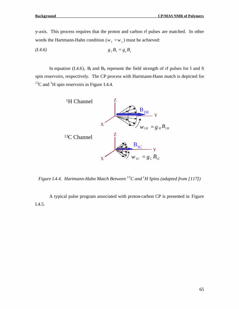
y-axis. This process requires that the proton and carbon rf pulses are matched. In other
words the Hartmann-Hahn condition ( sI ωω = ) must be achieved:
(I.4.6) ssII BB γγ =
In equation (I.4.6), BI and BS represent the field strength of rf pulses for I and S
spin reservoirs, respectively. The CP process with Hartmann-Hann match is depicted for 13C and 1H spin reservoirs in Figure I.4.4.
Figure I.4.4. Hartmann-Hahn Match Between 13C and 1H Spins (adapted from [117])
A typical pulse program associated with proton-carbon CP is presented in Figure
I.4.5.
Y
Z
X
Y
X
Z
B1H
B1C
HHH B11 γω =
CCC B11 γω =
1H Channel
13C Channel
Background CP/MAS NMR of Polymers
66
Figure I.4.5. CP Pulse Program (adapted from [134])
The Hartmann-Hahn condition therefore allows magnetization transfer between I
and S spin reservoirs. For such a magnetization transfer to be efficient however, the
interacting nuclei need to be in close spatial proximity, namely within 10 to 20 angstroms
[134]. In addition, the interacting nuclei need to be stationary with respect to the main
magnetic field [134]. Consequently both angstrom scale proximity and molecular rigidity
play an important role for CP. One easily foresees with these requirements that CP
constitutes an ideal tool for probing angstrom scale proximity and molecular scale
dynamics in solids. Consequently, probing intermolecular CP between two distinct
polymers is one of the most powerful relaxation experiments for assessing angstrom scale
miscibility as in polymer blends for instance. There exist a variety of well-established
relaxation measurements for probing polymer dynamics with CP/MAS NMR. The next
section examines the most common relaxation measurements that probe a specific range
of molecular motions or domain sizes. In that matter, particular attention shall be placed
on those relaxation experiments that reveal molecular scale morphology in polymer
blends since similar experiments may be envisioned for wood/adhesive systems.
I.4.4 CP/MAS NMR, a Probe of Polymer blend Morphology
The insight provided by CP/MAS NMR on polymer blend morphology stems
from relaxation rate/ dynamic domain size correspondence [114]. Understanding such
90° xCP
90° y Decouple
1H Channel
Repeat
CP
90° y
13 C Channel
RepeatAcquire
Background CP/MAS NMR of Polymers
67
equivalence warrants adequate design of CP/MAS NMR measurements for assessing
blend morphology on the desirable domain size.
I.4.4.1 Spin Dynamics and Polymer Blend Morphology
I.4.4.1.1 Fundamentals of Solid State Spin Relaxation
When an assembly of nuclear spins is in resonance, its population is biased from
Boltzmann’s distribution. Logically then, relaxation towards equilibrium ensues.
Relaxation may occur via spin-spin interactions at a characteristic time T2 (transverse
relaxation) or via spin- lattice interactions at a characteristic time T1 or T1ρ (longitudinal
relaxation) depending upon the reference frame considered (laboratory or rotating frame
respectively). Such relaxation mechanisms portray molecular scale dynamics. For
instance, megahertz frequency motions influence T1 while T1ρ is affected by mid-
kilohertz frequency motions [134]. Furthermore, owing to the abundance and spatial
proximity of protons in organic solids, additional relaxation mechanisms are effective.
CP is one example of such a mechanism and has already been discussed in detail. Let us
just recap that CP rates, TCH, are affected by spatia l proximity (10 to 20 angstroms) and
molecular rigidity as embodied by near static molecular motions [134]. Spin diffusion is
another common relaxation mechanism for organic solids. Spin diffusion refers to a
static magnetization transfer between abundant and adjacent protons. It is a non-motional
mechanism. Nevertheless, spin diffusion contributes to spin- lattice relaxations, T1 and
T1ρ. In other words, on top of the motional contribution to T1 and T1ρ, spin diffusion can
average molecular motions of the so-called coupled-spins [134]. It follows that distinct
nuclei (with distinct molecular motions) may have their T1 and T1ρ converge to a
common value by virtue of spin diffusion. In the same way that CP hinges upon spatial
proximity however, spatial proximity is required for effective spin diffusion. Namely,
spin diffusion occurs over nanometer scale domains. Conversely, spin diffusion is
ineffective across phase boundaries [134]. As a result, polymer blends that are
homogeneous on a nanoscale have their nuclei spin-coupled as reflected by a common
T1ρ. Phase separated polymer blends however, may exhibit distinct T1ρ for nuclei in
separate domains. Of course, the same reasoning applies to T1 rates since these are also
Background CP/MAS NMR of Polymers
68
affected by spin diffusion. However, T1 and T1ρ refer to different time scales and
therefore distinct domain sizes. Namely, T1 rates typically lie in the 100-500 ms range,
while T1ρ rates are on the order of 5-15 ms. Because spin diffusion occurs at
approximately 0.5-1 nm2/ ms in polymers, T1ρ may be associated with 2-30 nanometer
domains while T1 is relevant of 30 nanometer or greater domain sizes. Consequently,
morphological information can be obtained on specific domain sizes from T1 and T1ρ.
Let us now consider how practically, one may probe morphology in polymer blends with
relaxation mechanisms.
I.4.4.1.2 Relaxation Rate Measurements and Polymer Blend Morphology
Consider a polymer blend that comprises two spin reservoirs, a 13C and 1H spins
reservoir. All possible magnetization transfers and relaxation mechanisms are illustrated
in Figure I.4.6 for this polymer blend.
Figure I.4.6. Spin Relaxation in a CP/MAS NMR Experiment (adapted from [134])
The initial stage of a CP experiment is dominated by CP rate, TCH (typically in the
order of 0.1-1 ms). This results in 13C-detection enhancement as long as contact times
remain short enough i.e. in the order of TCH. With longer contact times (typically 5-15
ms), owing to rotating frame spin lattice relaxation, the 1H reservoir experiences a
decrease in magnetization. This results in a decay of 13C magnetization at the rate HT1ρ.
Hence the magnetization curve of 13C nuclei with respect to contact time bears the
competing effects of TCH and HT1ρ. In fact, both TCH and HT1ρ can be retrieved from the
magnetization equation in a variable contact time experiment (I.4.7) [134].
1H 13C
Lattice
HT1HT1ρ
TCH
CT1
CT2
CT1ρ
HT2
Background CP/MAS NMR of Polymers
69
(I.4.7) ( ) ( )CHH
TtTt
CHH
H
TT
TItI //
1
1 expexp 1 −−∗ −
−= ρ
ρ
ρ
In Equation (I.4.7), I(t) is the signal intensity at a contact time (t) and I* is the
corrected signal intensity for infinitely fast cross-polarization and infinitely slow proton
spin-lattice relaxation in the rotating frame. In Figure I.4.6, no discrimination between
the blend components has been considered. Oftentimes however, individual polymers
can be monitored from distinct 13C chemical shifts. As a result, variable contact time CP
experiments allow simultaneous monitoring of TCH and HT1ρ for each polymer. Simply
then, blend morphology can be determined from changes in the bulk polymer relaxation
rates. If polymers interact on the time scale (and domain size) characteristic of a
relaxation rate then this relaxation rate shall be altered as a result of blending. Changes
in TCH upon blending are thus indicative of angstrom scale interactions while changes in HT1ρ reflect nanometer scale interactions between polymers. This approach constitutes
the simplest experiment one can envision for assessing polymer blend morphology.
Another approach hinges upon the spatial requirements in static magnetization transfers,
CP and spin diffusion. In that matter, deuterium NMR experiments have been devised to
assess intermolecular CP in polymer blends [137]-[141]. Such experiments assess
intermolecular CP in blends where one polymer is fully deuterated. Recall that deuterium
is magnetically inactive and that 1H-13C CP occurs on 10 to 20 angstroms domains. In a
miscible blend of two dissimilar polymers, where one of the polymers is deuterated, i.e.
devoid of any protons, carbons in the deuterated polymer may be detected only through
CP from the protonated polymer. In an immiscible blend, the deuterated polymer
remains undetected because its 13C nuclei are too far removed from a proton source.
Hence, detection of a deuterated polymer in so designed polymer blends is evidence of
angstrom scale miscibility. Such experiments have been extensively utilized in the early
1980’s and remain one of the most powerful probes of angstrom scale morphology [137]-
[141]. In the same way, the spatial requirement inherent to spin diffusion has been
widely utilized to probe nanoscale morphology in polymer blends. The detection of a
unique HT1ρ , regardless of the 13C monitored, indicates nanoscale homogeneity. Distinct
Background CP/MAS NMR of Polymers
70
HT1ρ ‘s for 13C nuclei pertaining to distinct polymers on the other hand reveals nanoscale
phase separation. This approach is certainly attractive in that it does not require
deuterium labeling and can be carried out from simple variable contact time CP [135],
[136]. While these 3 approaches, molecular dynamics, intermolecular CP and spin
diffusion are the most common experiments for polymer blends, alternative experiments
can be envisioned. For instance, T1 measurements can be utilized to probe polymer blend
morphology on 30 nanometers and greater domain sizes [135]. Recently, the
development of two-dimensional pulses has granted novel probes of polymer blend
morphology [120]. Generally, 2D experiments examine the time dependence of 1H spin
diffusion between distinct regions of a polymer blend (mobile versus rigid for instance). 1H-Wideline separation or the WISE experiment is one example of a 2D experiment that
permits measuring the scale of heterogeneity in polymer blends [120]. Certainly also,
one foresees in the near future that an increasing number of pulse sequences will be
available for probing polymer blend morphology. In spite of CP/MAS NMR capabilities,
wood scientists have utilized such techniques with reserve. In recent years however, a
growing number of papers have been published, which demonstrate CP/MAS NMR value
for in-situ investigations of wood [128]. In the following section, significant CP/MAS
NMR studies on wood are reviewed. Special emphasis is placed on relaxation
measurements that give insight on wood morphology. The next section also examines the
capability of CP/MAS NMR to reveal molecular aspects of various treatments of wood
and adhesive treatment in particular. However, the reader is directed towards Gil et al.
for a more detailed survey of CP/MAS NMR application to wood and other
lignocellulosic materials [128].
I.4.4.2 Application of CP/MAS NMR to Wood
Nowadays, assignments of wood 13C chemical shifts are well established and are
exemplified with yellow-poplar CP/MAS NMR spectrum in Figure I.4.7 [121].
Background CP/MAS NMR of Polymers
71
Figure I.4.7. 13C CP/MAS NMR Spectrum of Yellow-poplar (Liriodendron tulipifera)
The spectrum is dominated by carbohydrate resonances at 63-66, 72-74, 83-89,
and 105 ppm. In particular, carbohydrate C4 and C6 appear in the 85-90 ppm and 63-66
ppm regions respectively. Carbohydrates C2, C3 and C5 on the other hand dominate the
72-74 ppm region. It can be noticed that C4 and C6 chemical shifts both comprise a sharp
resonance and a broader upfield resonance or shoulder in the case of the C6. The sharp
resonance stems from crystalline regions of cellulose (and that fraction of hemicellulose
that may be crystalline such as xylans ) and the upfield resonance arises from more
disordered amorphous regions [128]. Finally, a distinct resonance at 105 ppm is
characteristic of cellulose C1 and overlaps with that of hemicellulose C1 at 103 ppm.
Hemicellulose is largely manifest in the broad background between 50 and 90 ppm.
Hemicellulose acetyl groups can also be seen at 22 ppm (methyl carbon) and 175 ppm
(carbonyl carbon). Lignin contributes to the wood spectrum at 56 ppm and in the 130-
150 ppm region. The peak at 56 ppm corresponds to methoxyl groups and resonances at
122, 135, 153 ppm arise from unsubstituted, alkylated and oxygen-substituted aromatic
carbons respectively. Clearly evident with these assignments is CP/MAS NMR
capability to distinctively monitor in-situ wood polymers. As a result, fine structural
information can be obtained from CP/MAS NMR analysis of wood. For instance,
180 160 140 120 100 80 60 40 20 PPM
Background CP/MAS NMR of Polymers
72
quantitative CP/MAS NMR permits in-situ assessment of Syringyl/ Guaiacyl ratios for
lignin but also cellulose crystallinity [122], [123]. With this resolution of in-situ wood
polymers, CP/MAS NMR has emerged as an ideal probe of wood morphology and wood
polymer dynamics.
I.4.4.2.1 Use of Relaxation Measurements for Wood based Systems
Nuclear spin relaxation experiments have been widely utilized to characterize
wood morphology [124]. Newman for instance performed delayed-contact pulse
experiments and acquired distinct subspectra of wood for long and short TH1ρ’s [124]. In
this study, the short TH1ρ (mobile fraction) subspectrum comprises lignin and
hemicellulose, while cellulose appears in the long TH1ρ (rigid fraction) subspectrum
[125]. The occurrence of distinct TH1ρ for mobile and rigid wood components suggests
nanoscale phase separation between wood amorphous matrix and crystalline cellulose
phases. Tekely et al. on the other hand, reported identical TH1ρ values for wood polymers
thereby hinting towards phase homogeneity on a nanoscale [129]. Surprisingly, the same
authors measured distinct TH1 for all wood polymers, indicating phase heterogeneity on a
scale greater than 30 nanometers [130]. This controversy on wood morphology was
reconciled thanks to additional CP/MAS NMR analyses by Newman [126]. Newman
established that moisture plays a critical role on wood relaxation. Specifically, moisture
helps discriminate between cellulose and lignin TH1ρ ‘s [126]. Upon moisture uptake,
lignin TH1ρ decreases while that of cellulose increases [126]. Divergent TH
1ρ‘s with
increasing moisture content was ascribed to two mechanisms. On the one hand, moisture
alters cellulose microstructure from an amorphous to a more ordered state induced by
hydrogen bonding [127]. For lignin on the other hand, moisture enhances spin diffusion,
thereby decreasing its TH1ρ. Spin diffusion contribution to lignin TH
1ρ is clearly
evidenced by differences in TH1ρ ‘s between H2O and D2O moistened wood [126]. The
same comparison indicates no notable moisture induced spin diffusion for cellulose
[126]. With this thorough investigation of moisture effect on wood relaxation, Newman
has put an end to this controversy on wood morphology as detected by CP/MAS NMR.
Namely, under moist conditions, phase separation is indicated by distinct TH1ρ values for
crystalline and amorphous phases while under dry conditions homogeneous morphology
Background CP/MAS NMR of Polymers
73
is suggested from efficient spin diffusion. Other CP/MAS NMR investigations have
tackled the effect of various treatments on wood molecular packing. For instance, early
CP/MAS NMR studies have concentrated on the molecular impact of steam explosion
(SE) on wood morphology [129]. Steam explosion consists of contacting wood chips
with superheated steam under high pressure for a brief period of time. Upon abrupt
decompression, the chips are exploded. Steam explosion not only leads to condensation
of degradation products but also reduces wood polymer molecular mixing as evidenced
by distinct TH1ρ for steam exploded components [129]. Other treatments pertaining to the
manufacture of pulp and paper such as sulfonation and methylation have also been
studied by CP/MAS NMR [131], [132]. In that matter, Argyropoulos and coworkers
measured TH1 of sulphonated and methylated spruce pulps [131]. Interestingly, changes
in lignin TH1 upon sulfonation and methylation were found to parallel those in
carbohydrates. More specifically, both sulfonation and methylation appeared to decrease
wood polymers TH1 thereby indicating enhanced molecular mobility on the megahertz
frequency range [132]. Similarly, parallel trends for lignin and cellulose TH1’s with
changes in pH were observed for megahertz frequency motions [132]. As wood is treated
under alkaline conditions, wood functional groups are ionized and the resulting repulsive
forces enhance wood polymer mobility thereby allowing for shorter TH1. This effect is
and enolic hydroxyl groups are predominantly ionized while weakly acidic primary and
secondary hydroxyl groups remain minimally ionized. Hence the significant
enhancement in molecular mobility detected above pH 10 results from ionization of
specific functional groups [132]. Both studies are further interesting in that the parallel
trend for lignin and carbohydrates TH1 suggests molecular connectivities between wood
components [131], [132]. Thermal treatment is certainly the most common treatment
performed on wood. Thermal treatment is thought to cause several chemical changes.
On the one hand, organic acids released from hemicellulose are likely to cleave ligno-
polysaccharide complexes. On the other hand, condensation reactions may generate
secondary lignin-carbohydrates bonds. Kosikova et al. utilized TH1 measurements for
better understanding the influence of heat treatment on wood [133]. Alkaline
pretreatment was also investigated in this study. When thermal treatment followed a
Background CP/MAS NMR of Polymers
74
sodium hydroxide conditioning, cellulose crystallinity index was found to increase while
lignin degraded mainly through β aryl- linkage cleavage [133]. In addition, evidence for
lignin hydrogenation was found. The authors also proposed heat induced carbohydrate-
lignin linkages as a result of unique TH1ρ for lignin and amorphous cellulose in a model
lignin-carbohydrate compound [133]. While this study demonstrates the power of
CP/MAS NMR to elucidate chemical and morphological changes upon wood treatment, it
certainly emphasizes the complexity of chemical and morphological changes induced by
any treatment of wood. Hence, complementary information such as that obtained from
cross-polarization rates is useful for probing molecular order and packing in wood [146].
Let us recall that TCH, is a distance dependent phenomenon and is sensitive to near static
motions. It therefore reflects local packing arrangements as well as near-static motions.
Again, the influence of moisture content on wood polymer TCH has been the subject of
early CP/MAS analysis on wood treatment. Marcinko and coworkers reported faster
cross polarization rates for Aspen and Southern Pine polymers upon hydration [148].
Faster TCH rates were ascribed to increases in cellulose ordering and hydrogen bonding of
lignin [148]. This data is consistent with Newman’s interpretation of moisture effect on
wood polymers TH1ρ. More interesting, wood TCH has been shown to correlate with wood
dynamic modulus, thereby establishing a bridge between molecular arrangement and
macroscopic performance [146]. Such studies clearly indicate that TCH measurements are
well suited to probe the intimate environment and near static molecular motions of wood
polymers and their changes upon treatments. Along with TH1 and TH
1ρ measurements,
TCH measurements shall therefore be ideally suited for probing the morphology of wood/
adhesive interphases. In fact, the use of CP/MAS NMR relaxation time measurements
for probing wood bondlines is now well established.
I.4.4.2.2 Application of CP/MAS NMR Techniques for Wood/Adhesive Bondlines
In-situ wood adhesion mechanisms can be explored by directly investigating the
wood adhesive bondline. Because adhesives can be enriched in magnetically active
nuclei, fine structural and morphological information can be obtained from CP/MAS
NMR analysis of wood adhesive bonds [142]. The method has proved successful for in-
situ investigations of wood-isocyanate cure chemistry [143], [144]. In fact, semi-
Background CP/MAS NMR of Polymers
75
quantitative structural information can be obtained from CP/MAS NMR analysis of
wood-adhesive bondlines. As mentioned in chapter II-1, PF resin cure may be monitored
in-situ thanks to CP/MAS NMR [145]. The cure of PF resins proceeds via condensation
of hydroxymethyl groups to methylene bridges. In a CP/MAS NMR spectrum of a
wood-PF resin bondline, these functionalities can be resolved provided the resin is
enriched in 13C [145]. Hence, the proportion of methylene and methylol carbons can be
measured by integration of their respective signal [145]. Quantitative analysis
additionally requires the knowledge of TCH and TH1ρ relaxation times since both
relaxation rates control carbon magnetization in a CP experiment. More interesting on a
morphological standpoint, relaxation rates for adhesives and wood can be monitored from
CP/MAS NMR. For instance, it has been demonstrated that wood induces nanometer
scale heterogeneity in a PF resin network [145]. That is, while the neat PF resin exhibits
a similar TH1ρ value whether it is measured through the methylene or methylol carbon,
the TH1ρ from these two carbons diverges in wood-PF systems [145]. Similar phenomena
have been observed with isocyanates. With long curing time, nanometer scale
heterogeneity develops in an isocyanate bondline as evidenced by different TH1ρ for
distinct pMDI functionalities [150], [143]. While these studies essentially examine the
bondline from the standpoint of the adhesive, the reverse approach shall be similarly
fruitful. In other words, morphological information shall stem from changes in wood
polymer relaxation upon adhesive application. Such an approach has been taken by So et
al. to elucidate the effect of resole on wood microstructure [149]. Resole effect on
cellulose crystallinity appears to depend on the length of resin application on the
substrate. At short curing time, resole disrupts cellulose crystallinity while at longer
curing times recrystallization (presumably alkali induced transformation from cellulose I
to cellulose II) increases cellulose crystallinity [149]. Following this study, a number of
researchers have attempted to further elucidate adhesive impact on wood molecular
motions. Marcinko et al. reported for instance that liquid isocyanate binders decrease
wood components TH1ρ in Aspen wood thereby indicating intimate changes in the
nanometer scale environment of wood polymers [151]. Such an effect was ascribed to
pMDI ability to achieve intimate contact with wood polymers through plasticization. On
the other hand for yellow-poplar, liquid pMDI did not affect wood polymers TH1ρ [147].
Background CP/MAS NMR of Polymers
76
This discrepancy may arise from species dependence of pMDI penetration in wood. In
the same study the cured pMDI was reported to have no effect on wood polymers TH1ρ.
This again is at odds with Marcinko and coworkers results, which found that cured pMDI
also dramatically changes wood polymers TH1ρ [150]. In spite of some diverging results,
these morphological studies clearly establish the validity of NMR relaxation times for
assessing intimate mixing between wood polymers and adhesives. Overall, TH1ρ and TCH
measurements nicely complement each other to yield a molecular scale understanding of
adhesive penetration into wood.
Background References
77
I.5 REFERENCES
[1] White M.S., Influence of Resin Penetration on the Fracture Toughness of Bonded Wood, Doctoral Dissertation, Virginia Polytechnic Institute and State University, 1975.
[2] Siau J.F., Transport Processes in Wood, Springer-Verlag, New York, 1984.
[3] Nearn W.T., Application of the Ultrastructure Concept in Industrial Wood Products Research, Wood Science, 6 (3) 285, 1974.
[4] Nearn W.T., Wood-Adhesive Interface Relations, Conference on the Wood-Paint Interface, Berkeley, October 1964.
[5] Jonson S.E. and F.A. Kamke, Quantitative Analysis of Gross Adhesive Penetration in Wood Using Fluorescence Microscopy, J. Adhesion, 40, 47, 1992.
[6] Sernek M., J. Resnik and F.A. Kamke, Penetration of Liquid Urea-Formaldehyde Adhesive into Beech Wood, Wood Fiber Sci., 31 (1)41, 1999.
[7] Gray V.R., The Wetting, Adhesion and Penetration of Surface Coatings on Wood, Oil and Colour Chemists Association, 44, 756, 1961.
[8] White M.S., G. Ifju and J.A. Johnson, Method for Measuring Resin Penetration into Wood, For. Prod. J., 27, (7) 52, 1977.
[9] Saiki H., Electron Microscopy of Wood Cell Wall Impregnated with Aqueous Solution of Silver Nitrate, 19 (8) 367, 1973.
[10] Smith L.A., Resin Penetration of Wood Cell Walls, Implications for Adhesion of Polymers to Wood, Doctoral Dissertation, State University College of Forestry at Syracuse University, 1971.
[11] Robison R.G., Wood-Coating Interactions, Doctoral Dissertation, State University College of Forestry at Syracuse University, May 1972.
[12] Tarkow H., W.C. Feist and C.F. Southerland, Interaction of Wood With Polymeric Materials, Penetration Versus Molecular Size, For. Prod. J., 16 (10) 61, 1966.
[13] Siau J.F., The Swelling of Basswood by Vynil Monomers, Wood Sci. 1 (4) 250, 1969.
[14] Frazier C.E., Personal Communication.
[15] Mantanis G.I., R.A. Young and R.M. Rowell, Swelling of Wood. Part II. Swelling in Organic Liquids, Holzforschung, 48 (6) 480, 1994.
[16] Pizzi A., Advanced Wood Adhesives Technology, Marcel Dekker, Inc., New York, p89-151, 1994.
Background References
78
[17] Sellers T., Plywood and Adhesive Technology, Marcel Dekker Inc., New York, 1985.
[18] Astarloa-Aierbe G., J.M. Echeverria, M.D. Martin and I. Mondragon, Kinetics of Phenolic Resol Resin Formation by HPLC. 2. Barium Hydroxide, Polymer, 39 (15) 3467, 1998.
[19] Astarloa-Aierbe G., J.M. Echeverria, A Vazquez and I. Mondragon, Influence of the Amount of Catalyst and Initial pH on the phenolic Resol Resin Formation, Polymer, 41, 3311, 2000.
[20] Kaledkowski B. and J. Hetper, Synthesis of Phenol-Formaldehyde Resole Resins in the Presence of Tetraalkylammonium Hydroxides as Catalysts, Polymer, 41 (5) 1679, 2000.
[21] Freeman J.H. and C.W. Lewis, Alkaline-Catalyzed Reaction of Formaldehyde and the Methylols of Phenol, J. Am. Chem. Soc., 76, 2080, 1954.
[22] Caesar P.D. and A.N. Sachanen, Thiophene-formaldehyde Condensation, Ind. Eng. Chem., 40, 922, 1948.
[23] Grenier-Loustalot M.F., S Larroque and P. Grenier, Phenolic Resins: 1. Mechanisms and Kinetics of Phenol and of the First Polycondensates Towards Formaldehyde in Solution, Polymer, 35 (14) 3047, 1994
[24] Grenier-Loustalot M.F., S Larroque and P. Grenier, Phenolic Resins, 3. Study of the Reactivity of the Initial monomers Towards Formaldehyde at Constant pH, Temperature and Catalysts Type, Polymer, 37 (6) 939, 1996.
[26] Knop A. and L.A. Pilato, Phenolic Resins, Chemistry Applications and Performance, Springer-Verlag, New York, 1985.
[27] Pizzi A., Handbook of Adhesive Technology, Marcel Dekker Ed., New York, 1994.
[28] Miller H.A., Particle Board Manufacture, Noyes Data Corporation, New Jersey, 1977.
[29] Pizzi A., Wood Adhesives, Chemistry and Technology, Vol. 1 and 2, Marcel Dekker Inc., New York, 1983.
[30] Jones T.T., Preliminary Investigations of the Phenol-Formaldehyde Reaction, J. Soc. Chem. Ind., 65, 264, 1946.
[31] Maciel G.E., I. S. A. Chuang and L. Gollob, a Solid-State Carbon-13 NMR Study of Resol-Type Phenol-Formaldehyde Resins, Macromolecules, 17 (5) 1081, 1984.
Background References
79
[32] Zinke A, The Chemistry of Phenolic Resins and the Process Leading to their Formation, J. Applied Chem. (London), 1, 257, 1951.
[33] Lenghaus K., Qiao G.G. and D.H. Solomon, Model Studies of the Curing of Resole Phenol-Formaldehdye Resins Part 1. The Behaviour of Quinone Methide In a Curing Resin, Polymer 41 (6) 1973, 2000.
[34] Holopainen T., L. Alvila, J. Rainio and T.T. Pakkanen, Phenol-Formaldehyde Resol Resins Studies by 13C NMR Spectroscopy, Gel Permetation Chromatography, and Differential Scanning Calorimetry, J. Appl. Polym. Sci, 66 (6) 1183, 1997.
[35] So S. and A. Rudin, Analysis of the Formation and Curing Reactions of Resole Phenolics, J. Appl. Polym. Sci, 41 (1-2) 205, 1990.
[36] Schmidt R.G. and C.E. Frazier, Network Characterization of Phenol-Formaldehyde Thermosetting Wood Adhesive. Int. J. Adhes. Adhes. 18 (2) 139, 1998.
[37] Palmese G.R. and J.K. Gilham, Time-Temperature-Transformation (TTT) Cure Diagrams Relationship between Tg and the Temperature and Time of Cure for a Polyamic Acid/ Polyimide System, J. Appl. Polym. Sci., 34 (5) 1925, 1987.
[38] Young R.H., P.W. kopf and O. Salgado, Curing Mechanisms of Phenolic Resins, Tappi J., 64 (4) 127, 1981.
[39] Steiner P.R. and S.R. Warren, Rheology of Wood-Adhesive Cure by Torsional Braid Analysis, Holzforschung, 35 (6) 273, 1981.
[40] Kim M.G., W. L-S Nieh and R.M. Meacham, Study of Phenol-Formaldehyde Resol Resins by Dynamic Mechanical Analysis, Ind. Eng. Chem. Res. 30, 798, 1991.
[41] Kim M.G. and W. L.-S. Nieh and R.M. Meacham, Study on the Curing of Phenol-Formaldehyde Resol Resins by dynamic Mechanical Analysis, Ind. Eng. Chem. Res. 30, 4, 1991.
[42] Rials T.G. Cure Analysis of Phenol-Formaldehyde Resins by Microdielectric Spectroscopy, American Chemical Society Symposium Series 489, ACS, Washington D.C. 1989.
[43] Wang X.-M, B. Riedl, R.L. Geimer and A.W. Christiansen, Phenol-Formaldehyde Resin Curing and Bonding under Dynamic Conditions, Wood Sci. Technol., 30 (6) 423, 1996.
[44] Myers G.E., A.W. Christiansen, R.L. Geimer, R.A. Follensbee and J.A. Koutsky, Phenol-Formaldehyde Resin Curing and Bonding in Steam-Injection Pressing. I. Resin Synthesis, Characterization, and Cure behavior, J. Appl. Polym. Sci., 43, 237, 1991.
[45] Neiss T.G., Solution and Solid-State NMR Analysis of Phenolic Resin Cure Kinetics, Macromol. Symp. , 86, 117, 1994.
Background References
80
[46] Mizumachi H. and H. Morita, Activation Energy of the Curing Reaction of Phenolic Resin in the Presence of Woods, Wood Sci., 7, 3, 256, 1975.
[47] Pizzi A., B. Mtsweni and W. Parsons, Wood-Induced Catalytic Activation of PF Adhesives Autopolymerization vs. PF/ Wood Covalent Bonding, J. Appl. Polym. Sci., 52, 1847, 1994.
[48] Lu X. and A. Pizzi, Curing Conditions Effects on the Characteristics of Thermosetting Adhesives-Bonded Wood Joints, Holz-als Roh-Werkstoff, 56, 393, 1998.
[49] Lu X. and A. Pizzi, Curing Conditions Effects on the Characteristics of Thermosetting Adhesives-Bonded Wood Joints, Part 1: Substrate influence on TTT and CHT Curing Diagrams of Wood Adhesives, 56, 339, 1998.
[50] Garcia R and A. Pizzi, Crosslinked and Entanglement Networks in Thermomechanical Analysis of Polycondensation Resins, J. Appl. Polym. Sci., 70, 1111, 1998.
[51] Onic L., Bucur V., Ansell M.P., Pizzi A., Deglise X. and A. Merlin, Dynamic Thermomechanical Analysis as a Control Technique for Thermoset Bonding of Wood Joints, Int. J. Adhes. Adhes., 18, 89, 1998.
[52] Pizzi A., Lu X. and R. Garcia, Lignocellulosic Substrates Influence on TTT and CHT Curing Diagrams of Polycondensation Resins J. Appl. Polym. Sci, 71, 915, 1999.
[53] Ward I.M., Mechanical Properties of Solid Polymers, Second Ed., John Wiley & Sons Inc., New York, 1979.
[54] Ferry J.D., Viscoelastic Properties of Polymers, Second Ed. John Wiley & Sons, Inc., New York, 1970.
[55] Greener J., Relaxation Phenomena in Polymers: A Snapshot, PMSE News, incomplete reference, 1993.
[56] Ngai K.L. and R.W. Rendell, From Conformational Transitions in a Polymer Chain to Segmental Relaxation in a Bulk polymer, J. Non-Cryst. Solids 131-133, 942, 1991.
[57] Ngai K.L. and D.J. Plazeck, Identification of Different Modes of Molecular Motion In Polymers That Cause Thermorheological Complexity, Rubber Chemistry and Technology, 68, 376, 1995.
[59] Williams M.L., R.F. Landel and J.D. Ferry, The Temperature Dependence of Relaxation Mechanisms in Amorphous Polymers and Other Glass-forming Liquids, J. Am. Chem.Soc., 77, 3701, 1955.
Background References
81
[60] Doolittle A.K., Newtonian Flow. II. The Dependence of the Viscosity of Liquids on Free Space., J. Applied Phys., 22, 1471, 1951.
[61] Adam G. and J.H. Gibbs The Temperature Dependence of Cooperative Relaxation Properties in Glass-forming Liquids, J. Chem. Phys., 43 (1) 139, 1965.
[62] Mc Kenna, in Comprehensive Polymer Science, Vol. 2, Polymer Properties (ed. C. Booth and C. Price), Pergamon, Oxford, pp311-362 (Chapter 10), 1989.
[63] Kauzmann W., The Nature of the Glassy State and the Behavior of Liquids at Low Temperatures, Chemical Revs, 43, 219, 1948.
[64] Hodge I.A., Journal of Research of the National Institute of Standards and Technology, Adam-Gibbs Formulation of Enthalpy Relaxation near the Glass transition, 102 (2), 195, 1997.
[65] Vogel H., The Law of the Relation between the Viscosity of Liquids and the Temperature, Phys. Z., 22, 645, 1921.
[66] Fulcher G.S., Analysis of Recent Measurements of the Viscosity of Glasses. J. Am. Ceram. Soc., 8, 339, 1925.
[67] Tamman G. and W. Hesse, The dependence of Viscosity upon the Temperature of Supercooled Liquids. Z. Anorg. Allgem. Chemie,, 156, 245, 1926.
[68] Angell C.A., Journal of Research of the National Institute of Standards and Technology, 102 (2), 171, 2001.
[69] Angell C.A., Formation of Glasses from Liquids and Biopolymers, Science, 267, 1925, 1995.
[70] Hall C. K., and E. Hellfand, Conformational State Relaxation in Polymers: Time Correlation Functions, J. Chem. Phys., 77 (6) 3275, 1982.
[71] Williams, G.; Watts, D. C., Non-symmetrical Dielectric Relaxation Behavior arising from a Simple Empirical Decay Function, Trans Faraday Soc, 66 (1) 80, 1970.
[72] Ngai K. L., Modification of the Adam-Gibbs Model of the Glass Transition for Consistency with Experimental Data, J Phys. Chem B, 103, 5895, 1999.
[73] Plazeck D. J. and K. L. Ngai, Correlation of Polymer Segmental Chain Dynamics with Temperature-Dependent Time-Scale Shifts, Macromolecules, 24, 1222, 1991.
[74] Roland C.M. and K.L. Ngai, Segmental Relaxation and Molecular Structure in Polybutadienes and Polyisoprene, Macromolecules, 24, 5315, 1991.
[75] Roland C.M., Terminal and Segmental Relaxations in Epoxidized Polyisoprene, Macromolecules (25), 7031, 1992.
Background References
82
[76] Ngai K. L., and C. M. Roland, Chemical Structure and Intermolecular Cooperativity: Dielectric Relaxation Results, Macromolecules, 26, 6824,1993.
[77] Connolly M and F. Karasz, Viscoelastic and Dielectric Relaxation Behavior of Substituted poly(p-Phenylenes), Macromolecules, 28, 1872, 1995.
[78] Robertson C.G. and C.M. Roland, Breadth of the α Relaxation Function in 1,4-Polybutadiene, Macromolecules, 33, 1262, 2000.
[79] Roland C.M. and Ngai K.L., Segmental Relaxation in Miscible Polymer Blends, J. Rheol, 36 (8), 1992.
[80] Roland C.M. and K.L. Ngai, Dynamical Heterogeneity in a Miscible Polymer Blend, Macromolecules, 24, 226, 1991.
[81] Ngai K.L, C.M. Roland, J.M. O’Reilly and J.S. Sedita, Trends in the Temperature Dependency of Segmental Relaxation in TMPC/PS Blends, Macromolecules, 25, 3906, 1992.
[82] Roland C.M. and K.L. Ngai, Segmental Relaxation in Miscible Polymer Blends, J. Rheol. 36 (8) 1691, 1992.
[83] Vernel J, R.W. Rychwalski, V. pelisek, P. Saha, M. Schmidt and F. Maurer, Physical Aging in Poly(ethylene Oxide)/atactic-poly(methyl methacrylate) Blends, Thermochimica Acta, 342, 115, 1999.
[84] Robertson C.G and G. L. Wilkes, Glass-Formation Kinetics of Miscible Blends of Atactic Polystyrene and Poly (2, 6-dimethyl-1,4-phenylene oxide), Journal of Polymer Science: Part B: Polymer Physics, 39, 2118, 2001.
[85] Jensen R. E, C. E. Johnson and T. C. Ward, Investigation of a Waterborne Epoxy for E-Glass Composites, J. Polym. Sci., Part B: Polym. Phys., 38 (18), 2351, 2000.
[86] Yano S., H. Hatakeyama and T. Hatakeyama, Effect of hydrogen Bond Formation of Dynamic Mechanical Properties of Amorphous Cellulose, J. Appl. Polym. Sci., 20, 3221, 1996.
[87] Goring D.A.L., Thermal Softening of Lignin, Hemicellulose and Cellulose, Pulp Paper Mag. Can. 64 (12) T-51, 1986.
[88] Bradley S.A., and S.H.Carr, Effect of Fungal Degradation on Mechanical Properties of Cellophan, J. Polym. Sci., Polym. Phys. Ed., 14 (1), 125, 1976.
[89] Montes H., K. Mazeau and J.Y. Cavaille, Secondary Mechanical Relaxations in Amorphous Cellulose, Macromolecules 30, 6977, 1997.
[90] Montes H., K. Mazeau and J.Y. Cavaille, The Mechanical β Relaxation in Amorphous Cellulose, Journal of non-Crystalline Solids, 235-237, 416, 1998.
Background References
83
[91] Montes H. and J.Y. Cavaille, Secondary Dielectric Relaxations in Dried Amorphous Cellulose and Dextran, Polymer 40, 2649, 1999.
[92] Obataya E., M. Norimoto and B. Tomita, Mechanical Relaxation Processes in Wood in the Low-Temperature Range, J. Appl. Polym. Sci., 81 3338, 2001.
[93] Salmén N.L. and E.L. Back, The Influence of Water on The Glass Transition Temperature of Cellulose, Tappi, 60 (12) 137, 1977.
[94] Irvine G.M., The Glass Transitions of Lignin and Hemicellulose and Their Measurement by Differential Thermal Analysis, Tappi Journal 67 (5) 118, 1984.
[95] Salmén N.L., Thermal Softening of Paper: its Effect on Mechanical Properties, Pulp Paper Can. Trans Techn. Sec. 5 (3): TR 45, 1979.
[96] Olsson A.M. and L. Salmén , Humidity and Temperature Affecting Hemicellulose Softening in Wood, Proc. Int. Conf. of COST Action E8, June 16-17, Copenhagen, p.269, 1997.
[97] Salmén L., Viscoelastic Properties of In-situ Lignin Under Water Saturated Conditions, J. Mater. Sci., 19, (9), 3090,1984.
[98] Kelley S.S., T.G.Rials and W.G. Glasser, Relaxation Behaviour of the Amorphous Components of Wood, J. Mater. Sci., 22, 617, 1987.
[99] Salmén L., Directional Viscoelastic Properties of Wood, Progress and Trends in Rheology II, Proceedings of the Second Conference of European Rheologists, Prague June 17-20, p. 234, 1986.
[100] Wolcott M.P., F.A. Kamke and D.A. Dillard, Fundamental Aspects of Wood Deformation Pertaining to Manufacture of Wood-Based Composites, Wood Fiber Sci. 26 (4), 496, 1994.
[101] Furuta Y., M. Makinaga, H. Yano and H. Kajita, Thermal Softening Properties of Water Swollen Wood II. Anisotropic Characteristics of Thermal-softening Properties, Mokuzai Gakkaishi, 43 (1) 16, 1997.
[102] Östberg G. and L. Salmén , Characterization of Softening of Wood Fiber Wall Layers, Cellulose Chemistry and Technology, 21, 241, 1987.
[103] Olsson A.M. and L. Salmén , Viscoelasticity of In-situ Lignin as Affected by Structure, In: Viscoelasticity of Biomaterials, Eds. W.G. Glasser and H. Hatakeyama, American Chemical Society Symposium Series No 489, 133, 1992.
[104] Olsson A.M. and L. Salmén , The Effect of Lignin Composition on the Viscoelastic Properties of Wood, Nordic Pulp and Paper Research Journal, 3 (12), 140, 1997.
Background References
84
[105] Hamdan S., W. Dwianto, T. Morooka and M. Norimoto, Softening Characteristics of Wet Wood under Quasi Static Loading, Holzforschung, 54 (5) 557, 2000.
[106] Wennerblom M., A.M. Olsson and L. Salmén , Softening Properties of Earlywood and Latewood of Spruce, Nordic Pulp and Paper Research Journal, 4 (11) 279, 1996.
[107] Olsson A.M. and L. Salmén , Mechanical Spectroscopy- A Tool for Lignin Structure Studies, personal communication 2000.
[108] Salmén L. and A.M. Olsson, Interaction between Hemicelluloses, Lignin and Cellulose: Structure-Property Relationships, J.Pulp Paper Sci. 24 (99) 103, 1998.
[109] Lenth C.A. and F.A. Kamke, Moisture Dependent Softening Behavior of Wood, Wood and Fiber Science, 33 (3) 492, 2001.
[110] Nakano T. and Nakamura H., Viscoelasticity of Esterified Wood Specimens IV. The effect of Introduced Acyl Groups on Dynamic Mechanical Properties, Mokuzai Gakkaishi 21 (10) 820, 1987.
[111] Nakano T., Viscoelasticity of Esterified Wood Specimens IV. The effect of Molar Volume of Introduced Acyl Groups, Mokuzai Gakkaishi 33 (6) 472, 1988.
[112] Sugiyama m. and M. Norimoto, Temperature Dependence of Dynamic Viscoelasticities of Chemically Treated Woods, Mokuzai Gakkaishi 42 (11) 1049, 1996.
[113] Marcinko J.J., S. Devathala, P.L. Rinaldi, S. Bao, Investigating the Molecular and Bulk Dynamics of PMDI/Wood and UF/Wood Composites, Forest Products Journal, 48 (6) 81, 1998.
[114] Tycko R., Nuclear Magnetic Resonance Probes of Molecular Dynamics, Understanding Chemical Reactivity Vol. 8, Kluwer Academic Publishers, London, 1994.
[115] Havens J.R. and J.L. Koenig, Applications of High-Resolution Carbon-13 Nuclear Magnetic Resonance Spectroscopy to Solid Polymers, Applied Spectroscopy, 37, 3, 226, 1983.
[116] Silverstein R. M. and F. X. Webster, Spectrometric Identification of Organic Compounds, Sixth Ed. John Wiley& Sons, Inc, New York, 1998.
[117] Bruch M. D., NMR Spectroscopy Techniques, Practical Spectroscopy Series, Vol. 21, 2nd Ed., Ed. Marcel Dekker, Inc., New York, 1996.
[118] Schaefer J. and E. O. Stejskal, Carbon-13 Nuclear Magnetic Resonance of Polymers Spinning at the Magic Angle, J. Am. Chem. Soc., 98 (4) 1031, 1976.
[119] Kohler S. J., Introduction to NMR Spectroscopy of Solids, NMR Spectroscopy Application Note, IBM Instruments Inc. Incomplete Reference.
Background References
85
[120] Schmidt-Rohr K. and H. W. Spiess in “Multidimensional Solid-State NMR and Polymers”, Academic Press, New York, 1994.
[121] Kolodziejski V., J. S. Frye and G. E. Maciel, Carbon-13 Nuclear Magnetic Resonance Spectrometry with with Cross Polarization and Magic-Angle Spinning for Analysis of Lodgepole Pine Wood, Anal. Chem, 54, 1419, 1982.
[122] Newman R.H. and J.A. Hemmingson, Determination of the Degree of Cellulose Crystallinity in Wood by Carbon-13 Nuclear Magnetic Resonance Spectroscopy, Holzforschung, 44, 5, 1990.
[123] Manders W.F., Solid State 13C NMR Determination of the Syringyl/ Guaiacyl Ratio in Hardwoods, Holzforschung 41, 1, 1987.
[124] Newman R.H., Carbon-13 Nuclear Magnetic Resonance Studies of Molecular Motion in Wood and Paper, unknown Source.
[125] Newman R. H., Solid-State 13C NMR Spectroscopy of Multiphase Biomaterials, American Chemical Society, Viscoelasticity of Biomaterials, Ed. W. Glasser, 311, 1992.
[126] Newman R.H., Nuclear Magnetic Resonance Study of Spatial Relationships Between Chemical Components in Wood Cell Walls, Holzforschung, 46 (3) 205, 1996.
[127] Willis J.M. and F. G. Herring, Effect of Water in the 13C CP/MAS NMR Spectrum of White Spruce Wood, Macromolecules, 20, 1554, 1987.
[128] Gil A. M. and C. Pascoal Neto, Solid State NMR Studies of Wood and Other Lignocellulosic Materials, Annual Reports on NMR Spectroscopy, 37, 76, 1999.
[129] Tekely P. and M.R. Vignon, Cross-polarization/ Magic Angle Spinning 13C- NMR Characterization of Steam Exploded Poplar Wood, Journal of Chemistry and Technology, 7 (2) 215, 1987.
[130] Tekely P. and Vignon M.R. Proton T1 and T2 Relaxation Times of Wood Components Using 13C CP/MAS NMR, Journal of Polymer Science: Part C: Polymer Letters, 25, 257, 1987.
[131] Argyropoulos D.S. and F. G Morin, Probing the Macromolecular Structure of Wood and Pulps With Proton Spin-Lattice Relaxation Time Measurements in the Solid State, Wood Sci. Technol., 29, 19, 1995.
[132] Ahvazi B. and D. S Argyropoulos, Proton Spin-Lattice Relacation Time Measurements of Solid Wood and its Constituents as a Function of pH: Part I*, Wood Sci. and Technol., 34, 45, 2000.
[133] Kosikova B., M. Hricovini and C. Cosentino, Interaction of Lignin and Polysaccharides in Beech Wood (Fagus Salvatyca) during Drying Processes, Wood Sci. and Technol., 33, 373, 1999.
Background References
86
[134] Mehring M., Principles of High Resolution NMR in Solids, 2nd ed., Springer-Verlag, Berlin, 1983.
[135] Chu P.P and H.D. Wu, Solid State NMR Studies of Hydrogen Bonding Network Formation of Novolac Type Phenolic Resin and Poly(ethylene Oxide) Blend. Polymer 41, 101, 2000.
[136] Lee H.Y. and S.Y. Kwak, Dynamical heterogeneity and Molecular Mobility of hyper branched Poly(ether ketone)with Respect to the Homologous Linear, Polymer 42, 1375, 2001.
[137] Zhang X., A. Natansohn and A. Eisenberg, Intermolecular Cross-polarization Studies of the Miscibility Enhancement of PS/PMMA Blends through Ionic Interactions. Macromolecules 23 (2) 412, 1990.
[138] Schaefer J., M.Sefcik, Stejskal E. and R. McKay, Magic-angle Carbon-13 Nuclear Magnetic Resonance Analysis of the Interface between Phases in a Blend of Polystyrene with a Polystyrene-Polybutadiene Block Copolymer, Macromolecules 14 (1) 188, 1981.
[139] Parmer J., L. Dickinson, J. Chien and R. Porter, Macromolecules 20, 2308, 1987.
[140] Guo M. and H.G. Zachmann G. Intermolecular Cross-polarization Nuclear Magnetic Resonance Studies of the Miscibility of Poly(ethylene naphthalenedicarboxylate / poly(ethylene terephthalate) Blends, Polymer, 34 (12) 2504, 1993.
[141] Walton J., M. Lizak, M. Conradi, T. Gullion and J. Schaefer, Hydrostatic Pressure Dependence of Molecular Motions in Polycarbonates, Macromolecules 23 (2) 416, 1990.
[142] Frazier C. E., J. Ni and R. G. Schmidt, Applications of NMR Spectroscopy to the Analysis of Wood/Adhesive Bondlines, Adv. Lignocellulosic Charact., Ed. D. Argyropoulos, 145, 1999.
[143] Wendler S. L., and C. E. Frazier, The 15N CP/MAS NMR Characterization of the Isocyanate Adhesive Bondline for Cellulosic Substrates, J Adhes., 50 (2-3) 153, 1995.
[144] Wendler S. L., and C. E. Frazier, Effect of Moisture Content on the Isocyanate/Wood Adhesive Bondline by 15N CP/MAS NMR , J. Appl. Polym Sci., 61 (5) 775, 1996.
[145] Schmidt R. G. and C.E. Frazier, 13C CP/MAS NMR as a Direct Probe of the Wood-Phenol Formaldehyde Adhesive Bondline, Wood And Fiber Science, 30 (3), 250, 1998.
[146] Ni J. and C. E. Frazier, Molecular Correlations to Macroscopic Wood Performance Using CP/ MAS NMR, Holzforschung, 50 (4) 327, 1996.
[147] Frazier C.E. and J.Ni, On the Occurrence of Network Interpenetration in the Wood-Isocyanate Adhesive Interphase, Int. J. of Adhes. Adhes. 18, 81, 1998.
Background References
87
[148] Marcinko J. J., Measuring the Molecular Order and Dynamics of Hydrated Wood, Incomplete Reference, 1996.
[149] So S., J.W. The, A. Rudin, W.J. Tchir and C.A. Fyfe, Effect of Resole Adhesives on the Crystallinity of Cellulose, J. Appl. Polym. Sci., 39, 531, 1990.
[150] Marcinko J. J., P. L. Rinaldi and S. Bao, Exploring the Physicochemical Nature of PMDI/Wood Structural Composite Adhesion, For. Prod. J., 49 (5) 75, 1999.
[151] Marcinko J.J., W. H. Newman and C. Phanopoulos, Second Pacific Rim Bio-Based Composites Symposium, Vancouver, Canada, p. 286-293, 1994.
88
II DYNAMIC METHODS
Dynamic Methods Intermolecular CP Experiment
89
CHAPTER. II.1. INTERMOLECULAR CP AT THE WOOD/PF INTERPHASE
II.1.1 Introduction
Solid-state 13C NMR spectroscopy has been widely utilized for assessing
miscibility in polymer blends. In particular, the detection of intermolecular CP is
evidence for angstrom scale miscibility [1]-[5]. Intermolecular CP may be detected in
polymer blends that have been designed with specific deuterium labeling. In such
deuterium CP experiments, one polymer is hampered from intramolecular CP through
proton depletion while intermolecular CP remains possible between protonated and
perdeurated components provided that angstrom scale miscibility occurs [1]-[5]. The
objective of this study is to assess the feasibility of deuterium CP experiments for
detecting angstrom scale miscibility at the wood/PF interphase. Indeed, one can envision
a wood/PF composite, which is isotopically designed for detecting intermolecular CP
between wood and the PF resin. More precisely, in a wood/PF composite where the PF
resin is fully deuterated, detection of the PF resin would indicate intermolecular CP from
wood protons i.e. angstrom scale miscibility. For this experiment, complete deuteration
of the PF resin is required. In addition, 13C enrichment of the PF resin is necessary for
allowing resin detection within the composite [6]. Hence, for deuterium CP experiments
to be applicable to industrial composites, 13C and deuterium enriched PF resins need to be
synthesized. Owing to the distinct chemical shifts for PF hydroxymethyl and methylene
carbons in the CP/MAS NMR spectrum of wood/PF composites, formaldehyde is ideally
suited for bearing the 13C label. Unfortunately, doubly labeled formaldehyde (deuterated
and 13C enriched) is not commercially available and needs to be synthesized in the
laboratory. Hence the feasibility of intermolecular CP experiments in wood/PF
composites hinges in a first place upon the capability to synthesize formaldehyde-13C-d2.
Besides, a 13C and deuterium labeled PF resin cannot be synthesized with 100%
deuterium. Phenol for instance can be purchased with 98% deuterium labeling [7]. The
remaining 2% protons will generate intramolecular CP that is readily detected due to 13C
enrichment. Intramolecular CP may also arise from proton transfer at PF acidic sites
(Figure II.1.1) [8].
Dynamic Methods Intermolecular CP Experiment
90
Figure II.1.1. Exchangeable Protons in Hydroxymethyl Phenol
Recall that PF resoles are synthesized under basic conditions (pH typically greater
than 9). Under such conditions, phenolic hydroxyl groups are primarily in their ionic
form. Wood on the other hand is acidic. When a basic PF is put in contact with wood,
resin ionic sites may become predominantly protonated. In a deuterated PF resin then,
proton exchange with wood could generate some degree of intramolecular CP (Figure
II.1.2).
pKa ≅ 15
pKa ≅ 9
OH
CH2OH
Dynamic Methods Intermolecular CP Experiment
91
Figure II.1.2. Possible Proton Exchange between a Deuterated PF Resole and Wood
Therefore, in order to detect intermolecular CP between wood and a 13C and
deuterium enriched PF resin, reference to intramolecular CP must be made by evaluating
CP in a control PF-13C-d, which has been protonated at its acidic sites. With this control
PF resin, 13C-PF-D/H, the maximum intramolecular CP that could take place in a wood/ 13C-PF-D/H composite as a result of proton transfer can be quantified. It follows that
intermolecular CP may be detected by comparing CP in the neat control 13C-PF-D/H resin
to that in the wood/13C-PF-D/H composite. If cross-polarization in the 13C-PF-D/H is
enhanced by the presence of wood, then intermolecular CP from wood protons to the
Na
Na
Neat deuterated Alkaline PF
Acidic Wood Surface
Partially Protonated PF
OH
OH
13CD2
DO13CD2
O
13CD2
O
DO13CD2
OH OHOHOH CO OH
OH OHOHOH CO OH
Dynamic Methods Intermolecular CP Experiment
92
resin is taking place thus indicating angstrom scale proximity at the wood/PF interphase.
To date, no technique has been successfully applied to demonstrate wood/adhesive
interactions on the angstrom scale. Decisive steps towards the molecular engineering of
the wood/adhesive interphase could be taken with such a tool. It is therefore the
objective of this study to assess the feasibility of deuterium CP experiments for wood/PF
composites. In that purpose, the following tasks are addressed:
• Synthesis of 13C-d2 labeled paraformaldehyde
• Preparation of a control 13C PF D/H resin that permits reference for intramolecular CP
• Comparison of CP rates in the neat 13C PF D/H and in the wood/ 13C PF D/H composite.
II.1.2 Lab-Scale Synthesis of Paraformaldehyde
Schmidt determined the most viable route for the lab scale synthesis of doubly
labeled formaldehyde [15]. It consists of a gas phase oxidation of methanol over a
molybdenum-iron oxide catalyst. The reaction proceeds via a two-step mechanism
(Figure II.1.3).
Figure II.1.3. Reaction Mechanism for Methanol Oxidation into Aqueous Formaldehyde
with a Molybdenum-iron Oxide Catalyst ([15])
Initially, methanol is adsorbed onto the oxidized catalyst. The catalyst is
subsequently reduced and methoxy decomposition into formaldehyde and water follows.
The reaction is heat activated. An aqueous formaldehyde and paraformaldehyde slurry is
obtained. Figure II.1.4 depicts the experimental set up Schmidt utilized for this reaction.
Dynamic Methods Intermolecular CP Experiment
93
Figure II.1.4. Schmidt’s Experimental Set up for Formaldehyde Synthesis, Except F,
Which was Added in this Work ([12])
Liquid methanol is placed in a double neck flask immersed in a water bath (A).
Dry air is blown on methanol at a controlled rate and the methanol/air vapors are mixed
in a column through glass beads (B). The molybdenum iron oxide catalyst (C) is heated
through a heating tape (D) to a controlled temperature (E). When the methanol/air
mixture passes through the catalyst, methanol oxidation takes place thereby generating
vapors of water and formaldehyde. The reaction products pass through the reaction
vessel (F) and are finally condensed in the receiving flask (G), which is immersed in
liquid nitrogen (H).
In this work, Schmidt ‘s experimental set up was utilized, however a number of
modifications were applied. For instance, Schmidt first stabilized the catalyst temperature
to 340°C under constant air flow and then replaced the empty flask with one containing
approximately 1 ml of methanol [15]. Because the reaction is highly exothermic, a
Dynamic Methods Intermolecular CP Experiment
94
substantial increase in catalyst temperature (30°C) occurs during the course of the
synthesis. In the present work, it was deemed important to more thoroughly control the
catalyst temperature by incrementally adding small amounts of methanol. More
precisely, 0.25 ml aliquots of methanol were injected stepwise in the flask throughout the
course of the reaction. Between each methanol injection, the catalyst temperature was
allowed to stabilize back to the initial temperature. In addition, a heating tape was
wrapped on the vessel walls (F) in Figure II.1.4 past the catalyst so as to prevent
formaldehyde vapors from condensing on the glass wall ahead of the receiving flask.
This second heating tape was stabilized at 120°C.
Schmidt also proposed a drying procedure for obtaining paraformaldehyde from
the aqueous formaldehyde slurry. The drying procedure consisted of blowing dry air on
the formaldehyde solution overnight and subsequently vacuum drying for 4 hours [15].
With this procedure, Schmidt was able to achieve 49% yield of paraformaldehyde-13C-d2
from methanol-13C-d4 [15]. However, methanol-13C-d4 cost motivates efforts towards
improving the reaction yield. Hence, the first objective of this study has been to optimize
the synthesis of paraformaldehyde-13C-d2. Logically, optimization focused on methanol
conversion into formaldehyde and then on the drying procedure towards
paraformaldehyde.
II.1.2.1 Optimization of Methanol Conversion to Aqueous Formaldehyde
Experimental plans were designed with a view to optimizing the synthesis
parameters. The experimental set up was as in Figure II.1.4 and Schmidt ‘s procedure
was utilized except for the modifications mentioned above. Experimental details can be
found in reference [12]. Methanol purchased from Aldrich was used as received. The
Molybdenum-iron Oxide catalyst obtained from Neste Resins Corp, was manufactured by
Perstop Polyols. The catalyst was ground with mortar and pestle and particles with mesh
size greater than 18 only were utilized. Experimental plans were based on Taguchi
methods [22]. Taguchi methods help define the critical parameters and their optimum
level toward a desirable response [22].
Dynamic Methods Intermolecular CP Experiment
95
II.1.2.1.1 Principle of Taguchi Methods
Taguchi experimental plans are valuable tools for optimizing a procedure with a
minimum number of experiments [22]. External and internal factors are defined [22].
External factors are those experimental variables that may be adjusted, while internal
factors are inherent to the process and remain fixed. Distinct levels are assigned to the
external factors and a Taguchi experimental table is designed in accordance with the
number of factors and levels [22]. For instance, assessing two factors (A and B) at two
levels (1 and 2) along with their interaction requires a L22 experimental table, which
simply amounts to four experiments (Table II.1.1).
Table II.1.1. L22 Taguchi Experimental Table
Experiment Factors Levels Response
#1 A1 B1 A1B1 R1
#2 A1 B2 A1B2 R2
#3 A2 B1 A2B1 R3
#4 A2 B2 A2B2 R4
The influence of each factor at each level (and interaction) is computed from the
experimental response. For example, contribution of factor A at level 1, A1, is obtained
from the average response to experiments 1 and 2 (II.1.1). Similarly, the contribution of
A at level 2, A2, can be compiled from experimental responses(II.1.2).
(II.1.1) 2
211
RRA
+=
(II.1.2) 2
432
RRA
+=
Comparing contributions from distinct levels helps indicate the favorable level for
each factor. This is best visualized in a response plot such as in Figure II.1.5. In this
Dynamic Methods Intermolecular CP Experiment
96
particular response plot, A2 is clearly favorable towards maximal response while B bears
little influence on the response.
Figure II.1.5. Influence of Factors A and B on Response
A logical follow up for this response plot would consist of testing factor A in the
vicinity of level 2 while the B factor would be discarded.
II.1.2.1.2 Application of Taguchi Methods for Optimizing Formaldehyde Yield
Because oxygen/methanol ratio and catalyst are reported to be critical in methanol
oxidation towards formaldehyde, three parameters were defined as external factors [21]:
1) Catalyst temperature
2) Catalyst amount
3) Airflow rate
Successive Taguchi plans were performed, each of these assessing simultaneously
two factors at two levels with L22 experimental tables. For each experiment, the
response, formaldehyde yield, was measured by sodium sulfite titration [21]. The sodium
12 A
B0
20
40
60
80
100
Response
Levels
Factors
AB
Dynamic Methods Intermolecular CP Experiment
97
sulfite method consists of converting formaldehyde into base by reaction with 1M sodium
sulfite (Figure II.1.6).
Figure II.1.6. Formaldehyde Reaction with Sodium Sulfite (from [21])
The base is then titrated with an acid using a color indicator. In the present study,
0.1 N hydrochloric acid and thymophtalein were utilized. Each mole of formaldehyde
yielding one mole of sodium hydroxide, formaldehyde mass is defined as:
(II.1.3) MNVmgdeformaldehy ××=)(
In Equation (II.1.3), V is the volume of the HCl solution in milliliters, N its
normality and M the molar mass equal to 30.03 g/mol. Formaldehyde yield was
measured on a percent mole basis. Three successive Taguchi plans were undertaken.
• Experimental Plan #1
In the first experimental plan, catalyst amount, airflow rate and interaction
between these factors were considered. These factors were set at extreme levels in
comparison with Schmidt’s procedure (Table II.1.2) [15]. Catalyst temperature remained
fixed throughout experimental plans 1 and 2, at 340°C.
Table II.1.2. Table of Factors for Taguchi Plan #1
Catalyst amount (g) Airflow rate (ml/min)
Level 1 5 70
Level 2 20 210
The response of the L22 experimental table is presented in Table II.1.3.
OHCH2O Na2SO3 H2O NaOH CH2(NaSO3)
Dynamic Methods Intermolecular CP Experiment
98
Table II.1.3. Experimental Table and Responses for Taguchi Plan #1
Experiment Catalyst
amount (g)
Airflow rate
(ml/min)
Interaction
level
formaldehyde yield
(mole %)
#1 5 70 1 29.9
#2 5 210 2 44.4
#3 20 70 2 19.1
#4 20 210 1 13.8
It was found by plotting the table of response (Figure II.1.7), that both factors as
well as the interaction were critical to the reaction yield.
Figure II.1.7. Effect of Airflow rate, Catalyst Amount and their Interaction on
Formaldehyde Yield (Taguchi plan #1)
Catalyst amount appeared as the most critical factor with a 20% gain in
formaldehyde yield between level 2 (20g) and level 1 (5g). The interaction between
airflow rate and catalyst amount was the second most significant factor with level 2 being
the most favorable (i.e. high flow rate combined with low catalyst amount). Airflow rate
Cat
alys
tA
mou
nt
Air
Flo
w R
ate
Inte
ract
ion
120
204060
80100 Yield (%)
Factors
Levels
Dynamic Methods Intermolecular CP Experiment
99
also displayed a minor effect on formaldehyde yield with high flow rates being
preferable. In accordance with these results, a second Taguchi plan was undertaken.
• Experimental Plan #2
Table II.1.4 presents the levels that were selected for catalyst amount and airflow
rate in the second Taguchi plan.
Table II.1.4: Table of Factors for Taguchi Plan #2
Catalyst amount (g) Airflow rate (ml/min)
Level 1 4 130
Level 2 3 170
Figure II.1.8 reveals that the catalyst amount remained the most critical factor in
this second plan, with level 1 (3g) yielding a higher response than level 2. The flow rate
exhibited the same trend as that observed in plan #1, namely high flow rates (level 2
i.e.170 ml/min) were more favorable to formaldehyde yield than low flow rates.
Dynamic Methods Intermolecular CP Experiment
100
Figure II.1.8. Effect of Airflow rate, Catalyst Amount and their Interaction on
Formaldehyde Yield (Taguchi plan #2)
At these levels however, the interaction was no longer critical to formaldehyde
yield. One can also recognize that overall, the experimental conditions utilized in this
second Taguchi plan gave higher yields (60-80%) than those from Taguchi plan #1 (20-
40%). Clearly confirmed with this observation is the adequacy of the directions followed
as a result of Taguchi plan #1. These directions were pursued in a third Taguchi plan.
II.1.2.1.3 Experimental Plan #3
In Taguchi plan #3, catalyst amount was retained as a factor while assigned with
lower levels. The Airflow rate was no longer considered and remained at its optimum
level (170 ml/min) for all experiments. Rather, catalyst temperature was introduced as an
external factor (Table II.1.5).
Cat
alys
tA
mou
nt
Air
Flow
Rat
e
Inte
ract
ion
120
20406080
100 Yield (%)
Factors
Levels
Dynamic Methods Intermolecular CP Experiment
101
Table II.1.5. Table of Factors for Taguchi Plan #3
Catalyst amount (g) Temperature (°C)
Level 1 2.5 340
Level 2 1.5 280
Results from this third experimental plan are illustrated in Figure II.1.9.
Figure II.1.9. Effect of Catalyst Amount, Catalyst Temperature and their Interaction on
Formaldehyde Yield (Taguchi Plan #3)
At these levels, the factors assessed displayed a minor effect on formaldehyde
yield. However, low catalyst amounts (1.5g) appeared again slightly favorable to
formaldehyde yield. Catalyst temperature also had a minor effect on the reaction yield
with level 1 (340°C) being more favorable than level 2 (280°C). No statistical interaction
was found between catalyst amount and temperature at these levels. In any cases, all
experiments performed in this third plan gave yields above 80%. Additional experiments
were performed to further optimize catalyst temperature and amount but did not result in
any yield enhancement. Thus optimal conditions for converting 1 ml of methanol into
Catalystamount
CatalystTemp.
Interaction
1
20
20
40
60
80
100Yield (%)
Factors
Levels
Dynamic Methods Intermolecular CP Experiment
102
aqueous formaldehyde under the particular experimental set up ut ilized in this study were
finally defined as:
• Catalyst amount: 1.5g
• Catalyst temperature: 340°C
• Airflow rate: 170 ml/min
Using these conditions, 88% methanol conversion into aqueous formaldehyde was
achieved. Murray et al., whom Schmidt adapted its synthesis procedure, reports 79%
aqueous formaldehyde yield with this route [10]. Optimization efforts subsequently
focused on minimizing formaldehyde loss during the drying step towards
paraformaldehyde formation.
II.1.2.2 Optimization of the Drying Protocol towards Paraformaldehyde
Monomeric formaldehyde converts to paraformaldehyde through removal of
water (Figure II.1.10) [21]. The equilibrium depends on formaldehyde concentration [21].
Specifically, the greater the formaldehyde concentration, the more the equilibrium shifts
toward paraformaldehyde [21].
Figure II.1.10. Formaldehyde and Paraformaldehyde Equilibrium
Unfortunately, formaldehyde has a low boiling point (-19°C) and significant
formaldehyde loss occurs upon water evaporation [21]. In order to minimize
formaldehyde loss, various drying techniques were evaluated:
1. The reaction product was dried under vacuum for 4 hours (room temperature
and 0.1 mm Hg).
2. A steady air stream was blown on the reaction product overnight (at room
temperature) and procedure 1) followed.
3. Paraformaldehyde was added to the reaction product and procedure 2)
followed. Paraformaldehyde addition was intended to shift the equilibrium
(Figure II.1.6) towards paraformaldehyde formation.
4. The reaction product was freeze dried.
n (HO-CH2-OH) HO-(CH2O)n-H + (n-1) H2O
Dynamic Methods Intermolecular CP Experiment
103
These drying procedures were implemented on commercial formalin (37 weight
percent formaldehyde). Paraformaldehyde yield was measured on a weight percent basis.
Procedure 3) gave the highest yield of approximately 84%. Overall, methanol to
paraformaldehyde yields were approximately 64%. The second step of the study was
then undertaken, namely the preparation of a control PF destined to quantifying
intramolecular CP.
II.1.3 Preparation of a Control 13C PF D/H Resin
Thermodynamic considerations suggest that, in a wood/PF composite, angstrom
scale interactions are favored with a low molecular weight PF resin, which has significant
amount of monomers and dimers. It is therefore appropriate to utilize a low molecular
weight PF resin for assessing the feasibility of deuterium CP experiments at the wood/PF
interphase. In addition, the neat resin must provide a reference for quantifying
intramolecular CP that may arise from proton transfer with wood. Therefore a procedure
was developed for synthesizing a low molecular weight PF resin and protonating this
resin at its exchangeable sites. The procedures were developed using unlabeled reagents
and the resulting PF resin was characterized with common analytical techniques.
II.1.3.1 PF Resin Synthesis
Phenol crystals, 37% formaldehyde solution and 30% sodium hydroxide solution
were purchased from Aldrich and used as received. Phenol, formaldehyde and sodium
hydroxide were mixed in a triple neck flask in P: F: NaOH molar ratios of 1: 2: 0.2.
Distilled water was added so as to obtain a theoretical solid content of 55%. The reaction
flask, connected to a condenser, was immersed in a silicone oil bath at 80°C.
Polymerization was allowed to proceed under stirring for one hour under a steady flow of
N2 gas. The resulting PF resin had a number average molecular weight of 190g / mole
and a solid content of 44%. The resin had a pH of 9.5. The 13C NMR spectrum confirms
the low degree of condensation of the resin (Figure II.1.11). Namely, a minute signal is
apparent for the methylene carbon bridging two phenol rings (35 to 45 ppm). In addition,
significant signals for free formaldehyde (84 ppm) and hemiformal moieties (60-72 ppm
and around 90 ppm ) substantiate the low advancement of the polymerization. The
carbons in the 120-160 ppm range are aromatic carbons. The signals above 150 ppm
Dynamic Methods Intermolecular CP Experiment
104
arise from the carbon bearing the hydroxyl group i.e. the phenolic carbon. Overall, the
PF-Low mixture comprises essentially monomers and dimers of mono-, di- and tri-
substituted hydroxymethyl phenols.
Figure II.1.11. 13C NMR Spectrum of Low Molecular Weight PF Resole in D2O,
Internally Referenced to DSS (Sodium 2,2-dimethyl-2-silapentane-5-sulfonate).
An acidification procedure was then developed for mimicking the proton transfer
that could take place during application and cure of a deuterated resin on wood.
II.1.3.2 Acidification Procedure
The acidification procedure aimed at decreasing the resin pH to at least 4. In that
purpose, a 37 weight percent hydrochloric (HCl) solution was added dropwise in 1 g of
PF resin by means of disposable micro-capillaries. The pH was continuously monitored
during acidification. Typically, upon adding 20±10 µl of HCl solution, the PF resin
turned transparent and exhibited an abrupt drop to the pH range 1-3. In many trials, pH
200 150 100 50 0PPM
Methylene
bridges
Methylol
groups,
hemiformal
moieties and
methylene
Hemiformal
moieties
Ortho and para
free aromatic
carbons
Meta
aromatic
carbons
Phenolic
carbons
Free
formaldehyde
ppm
Dynamic Methods Intermolecular CP Experiment
105
control proved tedious and the acidified resin would gel or phase separate during
acidification. This is expected when one considers the pH dependence of PF
polymerization rate and the influence of alkali on PF solubility in water [11]. At such
acidic pH’s, the rate of PF polymerization is generally enhanced [11]. With care, the
acidification procedure was successfully achieved. The 13C NMR spectrum of the freshly
acidified PF resin indicates no significant advancement in the degree of condensation
(Figure II.1.12). In fact, this spectrum is the same as that for the PF resole except for the
upfield shift of the phenolic carbons by approximately 2 ppm. The chemical shifts for
phenol and resorcinol have been established to be pH dependent [13], [14]. This is
especially the case for carbons bearing the hydroxyl group, which exhibit lower chemical
shifts with reduced alkalinity [14]. The upfield shift observed for the phenolic carbons in
the acidified PF is therefore consistent with greater shielding as a result of protonation.
Figure II.1.12. 13C NMR Spectrum of Acidified PF Resole in D2O, Internally Referenced
to DSS.
Synthesis and acidification procedures were implemented on labeled reagents for
performing the deuterium CP experiment at the wood/13C-PF-D/H interphase.
200 150 100 50 0 ppm
Dynamic Methods Intermolecular CP Experiment
106
II.1.4 Intermolecular CP Experiments at the Wood/PF Interphase
With the capability to synthesize and protonate a 13C and deuterium enriched low
molecular weight PF resin, intermolecular CP experiments at the wood/PF interphase
were assessed.
II.1.4.1 Materials and Methods
II.1.4.1.1 Synthesis of Paraformaldehyde-13C-d2
Methanol-13C-d4 (99% 13C and 99% d4) was purchased from Cambridge isotopes
and used as received. From 5 ml labeled methanol, 3.7grams paraformaldehyde-13C-d2
were synthesized according to the procedure described in reference [12]. Figure II.1.13
represents the 13C NMR spectrum of the doubly labeled paraformaldehyde after
dissolution for 4 hours in D2O in a heated sealed tube. Two signals are evident at 80.8
and 84.6 ppm. The 80.8 ppm signal arises from deuterated 13C methylene glycol. It
consists of a pentet signal with an intensity pattern of 1: 2: 3: 2: 1. Deuterium is a spin 1
nucleus. The (2n+1) rule predicts that 2 deuterons create five distinct local fields for the 13C nucleus of methylene glycol. The observed splitting pattern therefore establishes
deuterium attachment on the methylene glycol carbon.
Figure II.1.13. 13C NMR Spectrum of 13C-d2 Paraformaldehyde in D2O , Internally
were purchased from Cambridge isotopes inc. Reagents were used as received. 0.5287
grams of lab-scale synthesized 13C-d2 paraformaldehyde were mixed with 1.142 grams
D2O in a sealed tube filled with N2 and submersed in an oil bath at 170°C. After 10
minutes of stirring the solution turned clear, indicating hydration of formaldehyde in
D2O. The formaldehyde-13C-d2 solution was utilized to synthesize a 13C-PF-D/H resin
according to the procedure described above. For the labeled resin, the synthesis was
performed under N2 gas. Immediately after the polymerization, 1gram of 13C-deuterated
PF resole was acidified with 20±10 µl of 37% HCl solution. Neat cured 13C-PF-D/H
samples and yellow-poplar/13C-PF-D/H composites were subsequently manufactured.
II.1.4.1.3 Preparation of 13C PF D/H Neat Samples and Yellow-poplar/ 13C PF D/H Composites
Extracted yellow-poplar (Liriodendron tulipifera) powder was utilized for the
manufacture of wood/13C-PF-D/H composites. Extraction was deemed necessary for
eliminating any intermolecular CP detection between wood extractives and the resin.
Hence, yellow-poplar chips were ground to mesh 40 and submitted to soxhlet extraction
in a series of solvents. Specifically, extraction in 50% aqueous acetone was repeated
three times, each time for a period of 24 hours. Extractions in 50% aqueous methanol
and 50 % aqueous tetrahydrofuran were subsequently performed over 12 hour periods.
The amount of extractives was not measured. The extracted yellow-poplar powder was
then dried in a desiccator over drierite for 48 hours. The final moisture content was 1.5%
approximately. Composites were manufactured by mixing 0.410 grams extracted yellow-
poplar powder with 0.604 grams 13C-PF-D/H in a vial thereby yielding 65% theoretical
resin solids on wood. In order to enhance resin diffusion and penetration into wood, the
mixture was allowed to stand at room temperature for 30 minutes prior to cure. Cure was
then performed by submersing the mixture in a vial in a silicone oil bath at 150°C for 15
minutes. Similarly, neat 13C-PF-D/H samples were prepared by curing the PF resin in a
Dynamic Methods Intermolecular CP Experiment
108
vial immersed in oil bath at 150°C for 15 minutes. The cured resin was then ground with
a pestle and mortar. Both composite and neat resin samples were vacuum dried (room
temperature and 0.1 mm Hg) overnight and kept in a dessicator with drierite until
CP/MAS NMR analysis.
II.1.4.1.4 13C CP/MAS NMR Measurements
Cross-polarization experiments were performed on a Bruker MSL-300 MHz
spectrometer using a 7 mm probenkopf MAS.07.D8 probe. The spectrometer frequency
was set at 75.47 MHz for 13C Nuclei and the spin locking frequency for the proton
channel was approximately 56 kHz. Adamantane was utilized for establishing the
Hartmann-Hahn match. Neat resin and composite powdered samples were packed in a
zirconium oxide rotor, sealed with a Kel-f cap. The samples were spun at 5 kHz ± 20 Hz.
A standard CP pulse with variable contact time wase performed. As many as 12 contact
times were utilized within the 0.1-12 ms range. For each contact time, 600 scans were
accumulated. The recycle delay was 3.75 s and the acquisition time was 50 ms. Three
neat 13C-PF-D/H resin samples and two wood/13C-PF-D/H composites were analyzed.
II.1.4.2 Results and Discussion
13C CP/MAS NMR spectra for the neat 13C-PF-D/H resin and the wood/ 13C-PF-D/H
composite are presented in Figure II.1.14. In both spectra, PF methylene carbons are
clearly detected in the 30-40 ppm region. This region comprises two overlapping
resonances, one around 31 ppm, which corresponds to ortho-ortho methylene bridges and
the other centered at 40 ppm, which is characteristic of para-para methylene bridges [19].
A resonance at 63 ppm arises from PF hydroxymethyl carbons. Additional peaks are
detected around 71 and 90 ppm. Signal intensities suggest that these peaks stem from
other formaldehyde-based chemical structures in the PF network. In fact, signals that
generally arise from the aromatic PF carbons (here without 13C label) and from the wood
polymers remain undetected in this spectrum, at least compared to the 100% 13C enriched
PF carbons. Similarly, spinning side bands that are typically generated from the aromatic
PF carbons are not apparent in the spectra. In a CP/MAS NMR study of PF resins,
Maciel ascribes resonances around 71 ppm to methylene carbons of ether structures [18].
Dibenzyl ether linkages are believed to form under acid condensation of PF resins [20].
Dynamic Methods Intermolecular CP Experiment
109
Hemiformal species may also contribute to the 71 ppm resonance. In fact, the small peak
centered at 90 ppm confirms the presence of hemiformal species. It is established from
solution 13C NMR that hemiformal moieties attached to phenolic rings appear in the
vicinity of 90 ppm [19].
Figure II.1.14. 13C CP/MAS NMR Spectrum of Neat 13C PF D/H (top) and 13C PF D/H /
Yellow-poplar Composite
Clearly from Figure II.1.14, 13C enrichment allows monitoring PF nuclei both in
the neat 13C-PF-D/H sample and in the wood/ 13C-PF-D/H composite. Detection of the resin
indicates that PF 13C nuclei are cross-polarized from a proton source in neat and
composite samples. A more informative characterization of CP behavior in both systems
is obtained by assessing magnetization of PF methylene carbons. In Figure II.1.15 the
logarithm of the normalized intensity of PF methylene carbon is plotted as a function of
contact time for neat resin and composite samples. The data are averages of 3 samples
for the neat 13C-PF-D/H and 2 samples for the wood/ 13C-PF-D/H composite. One sees on
Figure II.1.15 that at short contact times, the signal intensity rises rapidly to its maximum
value. The build up of the signal stems from cross-polarization between proton and 13C
nuclei. Therefore faster CP is evidenced when shorter contact times are required to
120 100 80 60 40 20
Neat Resin
Composite
ppm
Dynamic Methods Intermolecular CP Experiment
110
achieve maximum signal intensity. In that perspective, Figure II.1.15 indicates faster CP
of methylene carbons within neat 13C-PF-D/H resins than within yellow-poplar/ 13C-PF-D/H
composites. Cross-polarization between the resin and wood is therefore not evidenced.
Also apparent in this figure, is the effect of deuterium enrichment. Namely, at long
contact times (5-15 ms), 13C magnetization typically decreases as a result of proton spin
lattice relaxation in the rotating frame, HT1ρ.
Figure II.1.15. Magnetization Curve for Methylene Carbon (35 ppm) in Neat 13C-PF-D/H
Resin and in Yellow-poplar/13C-PF-D/H Composite
Spin diffusion is known to contribute significantly to HT1ρ relaxation. In
particular, the contribution of spin diffusion to HT1ρ in PF networks has been
demonstrated [16]. In Figure II.1.15, no loss of magnetization is evident at long contact
times. Deuterium enrichment acts to physically separate protons thereby hindering spin
diffusion. It is therefore not unexpected that ineffective spin diffusion hampers HT1ρ
relaxation in these systems.
Slower CP in composites than in neat resin samples suggests that intermolecular
cross-polarization between wood protons and PF resin does not occur in this particular
wood/ PF composite. Experimental conditions have been selected so as to favor
0 2 4 6 8 10 12 -3.0
-2.5
-2.0
-1.5
-1.0
-0.5
0.0
Neat Resin
Composite ln(I/I*)
Contact Time (ms)
Dynamic Methods Intermolecular CP Experiment
111
molecular scale interactions in the interphase (low molecular weight PF resin, significant
diffusion time of the PF resin in wood). Slower CP in the composite sample therefore
suggests that no miscibility on the 10-20 angstrom level is detected. However, an
additional parameter must be taken into account. Namely, CP efficiency not only
depends on proton spatial proximity but also on the molecular rigidity of the interacting
nuclei pair [9].
Cross-polarization is especially affected by near static molecular motions [9]. In
other words, the more rigid materials on the near static frequency scale cross-polarize
faster than mobile materials on this frequency scale. Therefore, changes in CP may also
stem from differences in near static molecular motions. When comparing a highly
crosslinked thermosetting resin in the neat state to that cured in the presence of wood,
differences in the network rigidity may occur. In fact, Schmidt demonstrated that wood
has a substantial influence on PF network molecular structure and dynamics [15]. When
comparing HT1ρ values for methylene carbons in neat cured resin and in wood/PF
composites, Schmidt evidenced a dramatic decrease of PF HT1ρ in the presence of wood.
For PF methylene carbons, decrease in HT1ρ is associated with lower network crosslink
density and lower glass transition temperature [16]. These observations indicate that PF
network mobility is enhanced when curing the PF resin in the presence of wood.
Although molecular motions probed by HT1ρ differ from those affecting CP, it can be
speculated that curing a PF resin in the presence of wood hinders its CP as a result of
lower molecular rigidity. Consequently, the present observation that wood delays cross-
polarization in the PF resin does not necessarily invalidate the hypothesis of angstrom
scale miscibility at the wood/PF interphase. Rather, it indicates that in wood/adhesive
systems, morphological information may be obscured by substantial differences in
molecular rigidities between neat resin and composite samples. Consequently, two
scenarios can equally be envisioned: 1) intermolecular CP between wood and the PF
resin is not detected because angstrom miscibility is not occurring in wood/PF systems.
2) intermolecular CP is inhibited in the composite sample because of increased network
motion caused by wood.
It is further interesting to recall a morphological difference between neat PF
networks and PF networks cured in the presence of wood. Namely, Schmidt et al.
Dynamic Methods Intermolecular CP Experiment
112
showed that wood induces phase heterogeneity in a PF network as revealed by distinct HT1ρ values for the methylene and hydroxymethyl carbons [17]. This dynamic
heterogeneity in composites contrasts with homogeneity that is observed in neat PF
networks [16]. The study suggested that hydroxymethyl carbons are more intimately
associated with wood polymers. Closer proximity is in favor of intermolecular CP
detection. On the other hand, closer association with wood polymers may alter the nuclei
dynamics more significantly. In such a case, morphological information would be
obscured to a greater extent than for the methylene carbon. In order to test this
hypothesis, intermolecular CP was assessed through PF hydroxymethyl carbon. Average
magnetization curves for hydroxymethyl carbons in neat 13C-PF-D/H resin and in the
yellow-poplar/ 13C-PF-D/H composite are compared in Figure II.1.16.
Figure II.1.16. Magnetization Curves for the Hydroxymethyl Carbons (65 ppm) in Neat 13C-PF-D/H Resin and Yellow-poplar/13C-PF-D/H Composite
In Figure II.1.16, one sees again that CP occurs faster in the neat 13C PF D/H resin
than in the composite thereby denying the occurrence of intermolecular CP detection.
0 2 4 6 8 10 12-3.0
-2.5
-2.0
-1.5
-1.0
-0.5
0.0
Neat Resin Composite
ln(I
/I*)
Contact Time (ms)
Dynamic Methods Intermolecular CP Experiment
113
This observation supports the hypothesis that significant dynamic changes between neat
PF resin and wood/PF composites obscure the morphological information typically
obtainable from deuterium CP experiments. It seems that deuterium CP experiments are
not suited for detecting angstrom scale morphological features of wood adhesive
composites.
II.1.5 Conclusion
In this study, the steps necessary for adapting deuterium CP experiments to
wood/PF composites have been completed. Namely, the in- lab synthesis of doubly
labeled formaldehyde has been revisited and optimized [12]. A PF resin with specific
isotopic design has been prepared in order to account for the complications of proton
transfer in deuterated resins. Comparing CP in neat control deuterated PF resins and
wood/PF composites did not indicate any intermolecular CP, whether the PF methylene
or hydroxymethyl carbon was probed. While detection of intermolecular CP would
reveal angstrom scale interactions, the opposite observation does not rule out angstrom
scale miscibility at the wood/PF interphase. Rather, the study suggests that
intramolecular CP in the neat resin and dynamic changes between neat resin and
composite obscure morphological information. In wood/adhesive systems, owing to the
substantial difference in component rigidity, CP efficiency is likely to be reduced by
molecular mobility. As a consequence, deuterium CP experiments used to detect
molecular miscibility in synthetic polymer blends cannot yield angstrom scale
morphology into wood-PF composites.
Dynamic Methods Intermolecular CP Experiment
114
II.1.6 References
[1] Zhang X., A. Natansohn and A. Eisenberg, Intermolecular Cross-polarization Studies of the Miscibility Enhancement of PS/PMMA Blends through Ionic Interactions. Macromolecules 23 (2) 412, 1990.
[2] Schaefer J., M.Sefcik, Stejskal E. and R. McKay, Magic-angle Carbon-13 Nuclear Magnetic Resonance Analysis of the Interface between Phases in a Blend of Polystyrene with a Polystyrene-Polybutadiene Block Copolymer, Macromolecules 14 (1) 188, 1981.
[3] Parmer J., L. Dickinson, J. Chien and R. Porter, Macromolecules 20, 2308, 1987.
[4] Guo M. and H.G. Zachmann G. Intermolecular Cross-polarization Nuclear Magnetic Resonance Studies of the Miscibility of Poly(ethylene naphthalenedicarboxylate)/poly(ethylene terephthalate) Blends, Polymer, 34 (12) 2504, 1993.
[5] Walton J., M. Lizak, M. Conradi, T. Gullion and J. Schaefer, Hydrostatic Pressure Dependence of Molecular Motions in Polycarbonates, Macromolecules 23 (2) 416, 1990.
[6] Frazier C.E., J. Ni and R.G. Schmidt, Applications of NMR Spectroscopy to the Analysis of Wood/Adhesives Bondlines, Advances in Lignocellulosic Characterization, Chapter 6, p145-156, Ed. D. S. Argyropoulos, Tappi press, Atlanta, 1999.
[7] Cambridge Isotopes Inc. Catalog, 1998-1999.
[8] Kresge A.J. and Y. Chiang, Journal of American Chemical Society, 89, 17, 4411-4417, 1967.
[9] Mehring M., Principle of High Resolution NMR in Solids, Second Ed., Springer-Verlag, New York, 1983.
[10] Murray A. and D. L. Williams, Organic Synthesis With Isotopes, Chapter 6, Part I. Compounds of Isotopic Carbon, p. 607, Interscience Publishers, New York, 1958.
[11] Pizzi A. and K.L. Mittal, Handbook of Adhesive Technology, Marcel Dekker, Inc., New York, p. 336, 1994.
[12] Schmidt R.G, M.P. Laborie and C.E. Frazier, Lab Scale Synthesis of Doubly Labeled Formaldehyde for Formaldehyde Based Wood Adhesives, Holzforschung, 54, 1999.
[13] Nakashima T. T. and Maciel G.E., Effects of pH on the Carbon-13 Magnetic Resonance Spectrum of Phenol, Applied Spectroscopy, 26 (2) 220, 1972.
[14] Christiansen A.W., Resorcinol-Formaldehyde Reactions in Dilute Solution Observed by Carbon-13 NMR Spectroscopy., Journal of Applied Polymer Science, 75, 1760, 2000.
Dynamic Methods Intermolecular CP Experiment
115
[15] Schmidt R.G., Aspects of Wood Adhesion: applications of 13C CP/MAS NMR and Fracture Testing, Doctoral Dissertation, Virginia Polytechnic Institute and State University, Doctoral Dissertation, p.92-106, January 30 1998.
[16] Schmidt R.G. and C.E. Frazier, Network Characterization of Phenol-Formaldehyde Thermosetting Wood Adhesive. Int. J. Adhes. Adhes. 18 (2) 139, 1998.
[17] Schmidt R.G. and C.E. Frazier, 13C CP/MAS NMR as a Direct Probe of the Wood PF Adhesive Bondline, Wood and Fiber Science, 30 (3), 250, 1998.
[18] Chuang I. S. and G.E. Maciel, 13C NMR Investigation of the Stability of Resol-Type Phenol-Formaldehyde Resin Toward Formalin, Toward Base, and toward Nonoxidizing or Oxidizing Acid, Macromolecules, 24, 1025, 1991.
[20] Grenier-Loustalot M-F. , S. Larroque and P. Grenier, Phenolic Resins: 1. Mechanisms and Kinetics of Phenol and of the First Polycondensates Towards Formaldehyde in Solution, Polymer, 35 (14) 3047, 1994.
[21] Walker, J. F. Formaldehyde. 3rd ed., R. E. Krieger Publishers. Huntington, New York. 1975.
[22] Peace, G. S., Taguchi Methods: a Hands-on Approach, Addison-Wesley, Reading Massachusetts, 1993.
Dynamic Methods Cooperativity Analysis for Lignin Glass Transition
116
CHAPTER. II.2. COOPERATIVITY ANALYSIS FOR LIGNIN GLASS
TRANSITION
II.2.1 Introduction
One objective of this research is to develop methodologies that probe the scale of
wood/adhesive interactions through molecular dynamics. Among polymer relaxation
mechanisms, the alpha relaxation, or glass transition, typically involves nanometer to
micron scale domains. In wood science, lignin glass transition constitutes the most
studied relaxation mechanism. Interest in the lignin glass transition arises from its impact
on the processing of several wood-based products (pulp and paper, wood-based
composites). Several studies indicate that the glass transition of lignin can be detected in-
situ [1], [14], [2]. It is important to emphasize however that the in-situ lignin glass
transition is largely influenced by the interactions and the associations with the other
wood components. In fact, the softening behavior of isolated lignin is dramatically
different from that of in-situ lignin, clearly indicating the contribution of all wood
components to lignin in-situ softening [20]. In the present study, the term in-situ lignin
glass transition therefore refers to the lignin segmental motion as influenced by the
plasticizing effect of wood carbohydrates for instance and other effects from interactions
with wood components.
In dry wood, lignin glass transition occurs in the vicinity of 200°C. Its in-situ
detection is therefore difficult without damaging the wood structure. However, lignin
glass transition temperature is dramatically reduced in plasticized wood. Depending
upon the wood species and the nature of the diluent, the lignin glass transition can be
decreased to the 60-90°C range [1], [14], [2]. Salmén was the first to apply the time-
temperature superposition principle (TTSP) for water-saturated wood around the lignin
glass transition [1]. Kelley et al. further determined the influence of moisture content on
wood softening and observed phase separation in the amorphous matrix of wood by
detecting distinct glass transitions for hemicellulose and lignin [2]. In addition, Kelley et
al. demonstrated that TTSP applies to the in-situ lignin transition for wood plasticized by
ethyl formamide [2]. Both studies indicated that the Williams-Landel-Ferry (WLF)
equation [3] provides a good treatment of wood viscoelastic properties above the lignin
Dynamic Methods Cooperativity Analysis for Lignin Glass Transition
117
glass transition [1]-[2]. The applicability of the WLF equation for plasticized wood
suggests that the empirical coupling model developed by Plazeck and Ngai may also be
suitable for describing wood viscoelastic behavior [5]. The reader is directed to Chapter
I-3 for a detailed review of the Ngai coupling model along with the concept of
intermolecular cooperativity. Briefly, deviations from Arrhenius behavior around the
glass transition can be related to intermolecular coupling between non-bonded
neighboring segments. At a temperature far above Tg (Tg + 80K), segmental relaxation is
independent of non-bonded segments and occurs via bond rotation with a characteristic
relaxation time, the primitive relaxation time [6]. The primitive relaxation time (τ0) is
therefore characteristic of conformational transition rates of an isolated chain. At much
lower temperatures, molecular motions are restricted by intermolecular cooperativity
between non-bonded segments. Hence, characteristic relaxation times in this temperature
region are retarded due to intermolecular coupling. The Ngai coupling model quantifies
the restriction in molecular motions induced by intermolecular coupling [5]:
(II.2.1) ( )[ ] ( )nn
c TnT −∗ −= 11
0 )(1)( τωτ
In equation (II.2.1), τ* represents the characteristic relaxation time under the
influence of molecular coupling at a given temperature T, τ0 is the primitive relaxation
time, n is the coupling constant and ωc represents the crossover frequency between time
domains for independent segmental relaxation on the one hand and cooperative
segmental relaxation on the other hand. The coupling constant, n, quantifies the extent of
intermolecular cooperativity among non-bonded segments and ranges from 0 to 1 with
high values representing a high degree of intermolecular cooperativity. Empirically,
Plazeck and Ngai determined that polymers cooled closer to thermodynamic equilibrium
obey the WLF form of the coupling model [5]:
(II.2.2)
−+
−−
=−
g
g
g
g
T
T
TTC
T
TTC
an
2
1
log)1(
Dynamic Methods Cooperativity Analysis for Lignin Glass Transition
118
In equation (II.2.2), the authors postulated empirical universal values of C1= 5.49
and C2=0.141, [5]. The coupling constant can therefore be retrieved by normalizing the
WLF shift factor to the fractional deviation from the Tg. In addition to quantifying
deviations from Arrhenius behavior, the coupling constant reflects the distribution of
relaxation mechanisms in the vicinity of the glass transition. In fact, for neat polymers,
the coupling constant correlates to the Kohlrausch-Williams-Watt (KWW) exponent, β ,
which describes the non-exponentiality of the alpha dispersion [7]:
(II.2.3) β−= 1n
Therefore, the coupling constant not only reflects the severity of the deviation
from an Arrhenius behavior, but also the distribution breadth of relaxation mechanisms
involved in the alpha relaxation. Polymers that display high intermolecular cooperativity
(high n value) around the Tg are characterized by a broad distribution of relaxation
mechanisms. On the other hand, polymers with little intermolecular cooperativity (low n
value) around the Tg are more dynamically homogeneous and display a more narrow
distribution of relaxation mechanisms. Typically, polymers have coupling constants in
the 0.35-0.75 range [4]. The widespread success of the coupling model for neat polymers
and more complex polymeric systems is well established and the reader is again referred
to chapter-I-2-A on that matter. Wood itself is a complex composite structure of
polymers. In spite of this complexity, universal viscoelastic models such as the TTSP are
suitable to describe the viscoelastic properties of wood and of lignin softening in
particular [1]. This fact suggests that the cooperativity analysis may also be applicable to
the in-situ lignin glass transition. Note however, that an in-situ analysis would reflect
lignin characteristics but also its association with other wood components. With the
feasibility of such an analysis, a novel tool would be available to investigate molecular
aspects of the amorphous wood matrix. Of particular interest for the present research, the
cooperativity analysis may provide an additional probe for interactions between wood
polymers and adhesives. The objective of the present study is to investigate the
feasibility of the cooperativity analysis on wood. Specifically the validity of the Ngai
coupling model for the in-situ lignin glass transition is investigated. In addition,
Dynamic Methods Cooperativity Analysis for Lignin Glass Transition
119
preliminary data are sought so as to establish whether such analyses could be applied to
wood/adhesive composites.
II.2.2 Materials and Methods
II.2.2.1 Materials
Two wood species were selected for analysis, these were yellow-poplar
(Liriodendron tulipifera), a hardwood, and Norwegian Spruce (Picea abies), a softwood.
Flakes with dimensions 3.5 mm in the radial direction, 0.85 mm in the tangential
direction and 10 mm in the longitudinal direction were manufactured from soaked wood
blocks using a disk flaker. These were manufactured from sapwood exclusively. For
yellow-poplar, the samples consisted of earlywood only, while in Spruce a small amount
of latewood was also sampled owing to the smaller annual rings (approximately 3 mm/
annual ring). The specimens were allowed to air dry to approximately 6-8% moisture
content. They were subsequently saturated in ethylene glycol. Ethylene glycol was
chosen as the diluent because of its high boiling point (approximately 150°C) thus
enabling subsequent viscoelastic measurements on a large temperature window. Sample
saturation in ethylene glycol consisted of immersing the sample in an ethylene glycol
bath that had been set up in open air and adjusted to a temperature of 120±3 °C. The
mass of ethylene glycol absorbed by wood was not measured. After conditioning the
sample for one hour in the ethylene glycol bath, the sample was submitted to viscoelastic
measurements. A minimum of five samples was prepared for each species.
II.2.2.2 Dynamic Mechanical Analysis (DMA)
Viscoelastic measurements consisted of DMA measurements with a Perkin Elmer
DMA 7e. The sample was tested in a dual cantilever beam mode along the grain.
Throughout DMA measurements the specimen remained immersed in ethylene glycol.
Viscoelastic measurements on immersed samples were afforded by using a Teflon cup
that was manufactured to fit in the instrument furnace. The Teflon cup was filled with
approximately 40 cm3 of ethylene glycol thus allowing submersion measurements with
regular dual cantilever beam clamps. During the measurements, evaporation of ethylene
glycol and vapor contamination of the DMA driveshaft was minimized by covering the
Dynamic Methods Cooperativity Analysis for Lignin Glass Transition
120
Teflon cup with aluminum foil. In addition, helium (flow rate of 70 ml/min) was utilized
as the purge gas. For each sample, DMA conditions were determined from consecutive
dynamic stress scans at 20°C and also at 120 °C. From these dynamic stress scans, a
strain level was selected for remaining in the linear viscoelastic domain at both
temperatures. Some samples did not afford a common strain level for linear
viscoelasticity at the two temperatures and were discarded. For the satisfactory samples,
the selected strain level did not exceed 0.1%. It was deemed important to perform the
high temperature dynamic stress scan (lignin in the rubbery state) just before the actual
viscoelastic measurements as a means to erase the sample thermal history. Hence,
following the dynamic stress scan at 120°C, the sample was cooled to 20°C at a
controlled rate (1.5°C/ min) while remaining in the ethylene glycol bath. Thereafter,
temperature scans were performed at the predetermined strain level with a static load of
120% of the dynamic load. Temperature scans were performed at a fixed frequency from
20°C to 120 °C using a heating rate of 2°C/min. Five measurement frequencies were
successively applied, namely 0.2, 0.6, 1, 2 and 6 Hertz. Between each temperature scan,
the sample was allowed to cool to 20° C at 1.5°C/min in the ethylene glycol bath. Hence
each of the successive temperature scans was preceded by the same thermal treatment
(same cooling rate after reaching the rubbery state of lignin).
II.2.2.3 Data Analysis
Fifth order polynomials were fitted to the log (E’)-temperature curves at the five
frequencies according to the procedure utilized by Olsson et al. (Figure II.2.1) [14].
Dynamic Methods Cooperativity Analysis for Lignin Glass Transition
121
Figure II.2.1. Polynomial fit for Storage Modulus versus Temperature at 5 Frequencies.
The polynomial fits were utilized to generate isotherms every 3°C (Figure II.2.2).
9.0
9.1
9.2
9.3
9.4
9.5
9.6
9.7
20 40 60 80 100 120
Temperature (°C)
Log
[E' (
Pa)]
0.2Hz0.6 Hz1 Hz2 Hz6 Hz
Dynamic Methods Cooperativity Analysis for Lignin Glass Transition
122
Figure II.2.2. Isotherms (3°C Increments) from 20 to 120°C Generated from Polynomial
Fit in Figure II.2.1
Isotherms were shifted horizontally on a frequency scale to a reference isotherm
and master curves of log (E’) were created. The reference temperature utilized for the
TTSP corresponded to the measured Tg at 2 Hertz and was selected as the inflection point
in the storage modulus-temperature curve. The inflection point was determined from
taking the minimum in the storage modulus derivative with respect to temperature. Shift
factor plots were created and the WLF constants were determined by taking the linear
part of the graph obtained from plotting (T-Tref)/ log aT versus (T-Tref) (Equation (II.2.4),
Figure II.2.3)
(II.2.4) 121 /))(/1(log/)( CCTTCaTT refTref −−−=−
9.0
9.2
9.4
9.6
Log E' (Pa)
log f (Hz)
-1 1
Dynamic Methods Cooperativity Analysis for Lignin Glass Transition
123
Figure II.2.3. Linearized WLF Form and Determination of C1 and C2 WLF Constants
Figure II.2.4 compares the experimental shift factor plot to the WLF equation.
Good agreement is found at temperatures above Tg.
y = -0.1383x - 7.4275R2 = 0.994
-16
-14
-12
-10
-8-60 -40 -20 0 20 40 60
(T-Tref) (°C)
(T-T
ref)/
log
a T (°
C)
Dynamic Methods Cooperativity Analysis for Lignin Glass Transition
124
Figure II.2.4. Typical Experimental Shift factor versus WLF fit for EG Plasticized Wood
The shift factor was normalized to the fractional deviation from the Tg yielding
cooperativity plots. The data analysis was performed for the individual samples but also
average cooperativity plots were constructed. Average cooperativity plots were
constructed after the method by Jensen [17]. Namely, the average Tg was utilized and for
each sample the shift factor data were recalculated at each value of (T-Tg)/Tg.
Cooperativity plots were then compared to the Ngai coupling model by determining the
best fit to Equation (II.2.2).
II.2.3 Results and Discussion
DMA of ethylene glycol plasticized Spruce and Yellow-poplar woods was
amenable for detecting the in-situ lignin glass transition. A tan delta peak appeared in the
range of 85-95° and was accompanied by a drop in the storage modulus (Figure II.2.5).
-6
-4
-2
0
2
4
6
8
-60 -40 -20 0 20 40 60
(T-Tg)
log
(aT)
WLFexperimental
Dynamic Methods Cooperativity Analysis for Lignin Glass Transition
125
Figure II.2.5. DMA Temperature Scan at 1Hertz for EG Plasticized Wood
For Spruce wood saturated in ethylene glycol and tested along the grain, a tan
delta peak characteristic of lignin softening has been reported at 84°C at 1 Hertz [12]. In
addition, it has been repeatedly observed that dynamic mechanical measurements of
wood along the grain yield higher Tg values than measurements across the grain [9], [13].
According to Furuta et al., the tan delta peak is shifted up by 10°C when wood is tested
along the grain versus test across the grain [11]. Salmén also reported a small difference
between the tan delta peak measured along and across the grain [9]. This anisotropic
behavior has been ascribed to artifacts on the measurements of dynamic moduli as a
result of fiber reinforcement[9]. Hence, the tan delta peak observed in this study in the
85-95°C for ethylene glycol swollen wood tested along the grain can be ascribed to the
in-situ lignin glass transition. It is known however that lignin in different locations of the
wood cell displays diverse softening behavior so that the softening observed in this study
reflects the average softening of lignin for bulk wood. While saturation in ethylene
glycol was efficient for detecting the in-situ lignin transition, the pretreatment in ethylene
glycol prior to DMA measurements (1 hour conditioning at 120°C) clearly affected the
9.0
9.2
9.4
9.6
0 20 40 60 80 100 120 140
Temperature (°C)
Log
E' (
Pa)
0.1
0.2
0.3
Tan
Del
ta
Dynamic Methods Cooperativity Analysis for Lignin Glass Transition
126
wood. One indication of the severity of the pretreatment was the brown discoloration of
the ethylene glycol bath utilized for sample conditioning. Organosolvolysis of wood by
ethylene glycol has long been recognized and is thought to involve the rupture of
glycosidic linkages in the holocellulose fraction as well as some dissolution of the lignin
fraction [19]. Therefore, the viscoelastic measurements performed in this study apply to
wood that has been partially degraded as a result of organosolvolysis by ethylene glycol.
With that treatment however, TTSP of ethylene glycol swollen wood was possible within
the frequency and temperature windows utilized in this study. As previously reported for
ethyl formamide and water plasticized wood, vertical shifting was not necessary to yield
smooth master curves [1], [2]. While a wide frequency window is desirable to perform
TTSP, experimental limitations hampered measurements on a greater frequency range.
More specifically, at frequencies higher than 6 Hertz, the system resonance frequency
approached that of the test frequency. It is generally recommended to perform
measurements at a frequency 10 times less than the system resonance frequency [10]. In
this study, the resonance frequency typically decreased from 120 Hertz to 80 Hertz as the
sample was heated from 20°C to 120°C. For some samples then, superposition at the
highest temperatures proved difficult, presumably owing to the system resonance
frequency approaching the testing frequency. In this respect, thicker samples would
likely permit a wider frequency range. However, because this study intended to be
applicable to wood/adhesive interphases, thin specimens were preferred. Thin wood
specimens should be more amenable to a uniform distribution of the adhesive throughout
the thickness of the flakes. In any case, for most samples the construction of smooth
master curves over the entire temperature window and the frequency window utilized in
this study was possible (Figure II.2.6).
Dynamic Methods Cooperativity Analysis for Lignin Glass Transition
127
Figure II.2.6. A Typical Master Curve for Ethylene Glycol Plasticized Wood
The ability to create smooth master curves associated with a “smooth” shift factor
(i.e. no abrupt change in curvature) indicates that only one mechanism of motion is
probed, lignin glass transition in this particular case. The reproducibility of the master
curves can be appreciated by creating average master curves for the yellow-poplar and
spruce wood specimens. For that purpose, the individual master curves were vertically
shifted to the same average modulus value at the reference temperature. Figure II.2.7 and
Figure II.2.8 represent the superposition of all individual master curves for spruce and
Dynamic Methods Cooperativity Analysis for Lignin Glass Transition
128
Figure II.2.7. Average Master Curve for Five Different Samples of EG Plasticized
Spruce
-6 -4 -2 0 2 4 6 9.0
9.2
9.4
9.6
log [ E' (Pa) ]
log [f (Hz) ]
Dynamic Methods Cooperativity Analysis for Lignin Glass Transition
129
Figure II.2.8. Average Master Curve for Six Different Samples of EG Plasticized Yellow-
poplar
Considering the natural variability of wood, a good reproducibility is observed
especially in the case of Spruce Wood. Average Tg and WLF constants are presented in
Table II.2.1. In addition, the apparent activation energies at the Tg have been calculated
from the WLF constant as:
(II.2.5) 22
1 /303.2)/1()(ln
)( CTRCTdad
RTE gT
ga ==
Where R is the universal gas constant.
-6 -4 -2 0 2 4 6 9.0
9.2
9.4
9.6
log [ E' (Pa)]
log [ f (Hz)]
Dynamic Methods Cooperativity Analysis for Lignin Glass Transition
130
Table II.2.1. Viscoelastic Properties of EG Plasticized Spruce and Yellow-Poplar Woods
Derived from DMA Raw Data and WLF analysis (Standard Deviations in Parenthesis)
Spruce Yellow-poplar
Number of Samples 5 6
Tg @ 0.2 Hz (°C) 65 (7) 64 (4)
Tg @ 0.6 Hz(°C) 68 (5) 67 (4)
Tg @ 2 Hz (°C) 74 (3) 71 (4)
Tg @ 6 Hz (°C) 77 (4) 75 (4)
C1 -9.4 (1.3) -9.4 (2.2)
C2 87 (15) 78 (21)
Ea (@Tg) (kJ/mol) 252 (21) 274 (12)
Note that the reported Tg values in Table II.2.1 arise from the storage modulus
inflection point rather than the tan delta peak. The storage modulus inflection point
yields Tg that are typically 10°C lower than that obtained from the tan delta peak. Table
II.2.1 indicates similar Tg values for spruce and yellow-poplar woods albeit a trend for
higher Tg values in spruce may be found for the highest frequencies. Alpha relaxations
have activation energies typically greater than 100 kJ/mol. The activation energies
measured in this study for Spruce and Yellow-poplar woods are in the vicinity of 250
kJ/mol thus confirming the signature of an alpha relaxation. For ethylene glycol
plasticized spruce wood, the apparent activation energy of the glass transition has been
estimated to 190 kJ/mol using an Arrhenius equation [12]. It has also been reported for
several wood species that activation energies derived from the Arrhenius equation are 10
to 40 kJ/mol lower than those calculated from the WLF equation [14]. The activation
energies measured in this study are therefore consistent with those reported in the
literature. A one tail t-test was performed in order to determine whether the Tg measured
at 2 Hertz (reference temperature for the WLF analysis) for Spruce was greater than that
for yellow-poplar. The p-value of 0.11 indicated that the glass transition temperature of
Dynamic Methods Cooperativity Analysis for Lignin Glass Transition
131
Spruce wood might be slightly higher than that of yellow-poplar; but the difference was
not highly significant. Typically, softwood species exhibit higher lignin Tg than
hardwood species [14], [16]. Higher softening temperatures for lignin softwoods have
been ascribed to structural differences between softwood and hardwood lignins.
Softwood lignins are built upon guaiacyl units, which are more prone to yield a highly
condensed lignin structure. Hardwood lignins on the other hand comprise an equal
mixture of syr ingyl and guaiacyl units (and p. hydroxyphenyl units to a lower extent)
whose pendant methoxyl groups may hinder a highly condensed state of lignin [14].
Cooperativity plots were constructed by normalizing the shift factor to the
fractional deviation from the Tg. In a first attempt to evaluate the Ngai coupling model
on wood, cooperativity plots were constructed over the entire temperature range utilized
in this study. Figure II.2.9 compares the measured shift factor over the entire temperature
range to the best fit provided by the coupling model.
Figure II.2.9. Evaluation of the Ngai Coupling Model (Equation (II.2.2)) for EG
Plasticized Wood from 20 to 120°C
-0.15 -0.10 -0.05 0.00 0.05 0.10 0.15
-4
-2
0
2
4
6
Experimental dataNgai Coupling Model
log aT
(T-Tg)/ Tg
Dynamic Methods Cooperativity Analysis for Lignin Glass Transition
132
The coupling model fails to describe the cooperativity plot over the entire
temperature window. However, it must be kept in mind that the coupling model in its
“universal” form (Equation (II.2.2)) has been empirically developed for polymers, which
were slowly cooled into the glassy state closer to equilibrium [5]. Low free volume in
the glassy state is known to delay structural relaxation, which is necessary for
approaching equilibrium as required for the Ngai coupling model. Structural relaxation
may be all the more delayed if the polymer under probe is highly condensed or
crosslinked. Such a phenomenon has been observed in epoxy resins [17]. For epoxy
resins, the coupling model was found applicable only to experimental data above the Tg,
that is when fast structural relaxation towards equilibrium is possible [17]. In this study,
wood samples were allowed to cool at a controlled rate of approximately 1.5°C/min. It
may be that in the glassy state, lignin is restricted from approaching equilibrium. Hence,
evaluating the Ngai coupling model at temperatures above Tg appeared more appropriate
in the case of lignin. In that temperature range, the Ngai coupling model provides a good
fit to the cooperativity plot, Figure II.2.10.
Dynamic Methods Cooperativity Analysis for Lignin Glass Transition
133
Figure II.2.10. Evaluation of the Ngai Coupling Model for EG Plasticized Wood above
Lignin Tg
The fit in the high temperature range is all the more remarkable considering the
complexity of the wood structure. For each sample the coupling constant was retrieved
from the best fit to equation (II.2.2). The average Tg utilized for the cooperativity
analysis and the average coupling constants for yellow-poplar and spruce wood are
summarized in Table II.2.2. Table II.2.2 also presents a χ2 value for the goodness of the
fit to Ngai coupling model obtained from the average cooperativity plots (Figure II.2.11).
The χ2 value represents the sum of the squared differences between theoretical and
experimental data. Small χ2 values are therefore indicative of a good fit.
-0.02 0.00 0.02 0.04 0.06 0.08 0.10 0.12 0.14
-3
-2
-1
0
1
Experimental Data Ngai Coupling Model
log aT
(T-Tg)/T g
Dynamic Methods Cooperativity Analysis for Lignin Glass Transition
134
Table II.2.2. Cooperativity Constants and Reference Tg for EG Plasticized Spruce and
Yellow-poplar Woods (standard error in parenthesis)
Spruce Yellow-poplar
Reference Tg (°C) 74.4 (2.9) 71.3 (4.3)
N 0.13 (0.05) 0.19 (0.04)
χ2 0.006 0.005
In-situ lignin softening in ethylene glycol swollen yellow-poplar exhibits a
coupling constant of 0.19 ±0.04 while for spruce wood the coupling constant averages
0.13±0.05. Such measured n values for in-situ lignin appear small compared to those
typically encountered in synthetic polymers. For example, poly(vinyl-methyl-ether) has a
coupling constant of 0.5 and the more polar poly (vinyl-chloride) has a coupling constant
of 0.77. Two experimental conditions are believed to contribute to low measures of the
coupling constants in this study. First of all, saturation of wood in ethylene glycol
certainly creates free volume, which in turn decreases intermolecular cooperativity.
Recall that conditioning in EG depresses lignin glass transition from 200°C to
approximately 75°C. Lignin is therefore dramatically plasticized in this study. Second,
the selection of Tg influences to some extent the absolute cooperativity plots and the
determination of the coupling constant. The glass transition temperature is typically
determined as the onset of ∆Cp increase in DSC temperature scans at 10K/min. While in-
situ lignin glass transition has been reported to be detectable by DSC, it is notoriously
difficult [2], [18]. Another convention consists of determining Tg from DMA
temperature scans at a frequency corresponding to τ*= 100s, i.e. a much lower frequency
than that utilized in the present study. Unfortunately, instrumental limitations hampered
measurements at such a low frequency. Therefore, in this study, DMA scans at 2 Hertz
were utilized for selecting the reference glass transition temperature needed for the
cooperativity analysis.
Dynamic Methods Cooperativity Analysis for Lignin Glass Transition
135
Because the same conventions were applied to construct cooperativity plots for
yellow-poplar and for spruce, the comparative value of the analysis is preserved. Figure
II.2.11 presents the average cooperativity plots obtained for spruce and yellow-poplar. A
steeper temperature dependence of relaxation is suggested for yellow-poplar than for
spruce, albeit standard deviations are large. In fact, a t-test revealed no significant
difference between the coupling constant obtained for spruce wood and for Yellow-
poplar (p = 0.26).
Figure II.2.11. Comparison of Average Cooperativity Plots for Spruce (5 Different
Samples) and Yellow-poplar (6 Different Samples)
While there is for these two species no significant difference for lignin in-situ
cooperativity, the applicability of the cooperativity analysis suggests that it would be a
suitable tool for investigating in-situ molecular features. In fact a systematic study of the
influence of lignin composition on intermolecular cooperativity would be of great value
to further understand the molecular aspects of in-situ lignin relaxation. Such a
-0.02 0.00 0.02 0.04 0.06 0.08 0.10 0.12
-3
-2
-1
0 Spruce Poplar
Log
(aT)
(T-Tg)/Tg
Dynamic Methods Cooperativity Analysis for Lignin Glass Transition
136
systematic study has evidenced a correlation between lignin glass transition temperature
and methoxyl content and similar approaches can be envisioned with the cooperativity
analysis [14], [15]. Besides, wood is a composite structure in which the lignin-
hemicellulose amorphous matrix is constrained within rigid cellulose fibers. Therefore, it
is likely that intermolecular cooperativity measured within bulk lignin phases is largely
influenced by lignin interactions with the surrounding polymers. For instance, lignin is
covalently linked with hemicellulose. Hemicelluloses are to a large extent responsible
for the depression of lignin glass transition when comparing in-situ lignins and isolated
lignins [20]. No doubt then that hemicelluloses also affect the intermolecular
cooperativity measured around the in-situ lignin glass transition. Furthermore
hemicelluloses are intimately connected to cellulose through hydrogen bonding. Such
interactions are dynamic. Again the cooperativity analysis, albeit applied around lignin
in-situ softening is likely sensitive to these dynamic interactions. One could envision for
instance that the constraint imposed by cellulose fibers on the lignin- hemicellulose
matrix enhances intermolecular cooperativity within lignin phases. In that matter,
intermolecular cooperativity appears as a potential tool to provide further insight on the
in-situ molecular arrangement of wood polymers. More specifically, the impact of the
surrounding environment on lignin morphology could be assessed by evaluating the
effects of wood anisotropy on intermolecular cooperativity. If wood anisotropy were
found to influence intermolecular cooperativity, indication for some molecular
orientation in the amorphous matrix of wood would be provided. There is therefore great
potential and certainly great information yet to be learned from the cooperativity analysis
of wood from various species and in various environments. However, another objective
of this study was to determine if viscoelastic measurements may also be suitable for
characterizing the in-situ lignin glass transition in wood-PF composites. In that purpose,
preliminary data were obtained on wood–PF composites. The reader is directed to
chapter III-1 for a detailed description of the composite manufacture. Temperature scans
were thus performed under similar experimental conditions as those described for the
neat wood samples.
Dynamic Methods Cooperativity Analysis for Lignin Glass Transition
137
Figure II.2.12. DMA Temperature Scan of a Wood-PF composite (@ 0.2 Hertz)
Figure II.2.12 illustrates the Tan Delta and Storage Modulus data for a PF
composite plasticized in Ethylene glycol. The composite comprises 40% resin solids on
wood. A clear drop in modulus is evident in Figure II.2.12 and is associated with a tan
delta peak. The damping peak may be ascribed to in-situ lignin softening albeit again
caution is required in any strict assignment. Again, while wood main softening is
generally ascribed to lignin (for the particular conditions utilized in this study), it is well
established that lignin association with carbohydrates has a substantial effect on its
softening temperature [20]. Considering the high resin solids on wood, it is also possible
that some fraction of the PF resin participates in the softening. This is especially true
that PF resins are very similar in structure to lignin. In fact just as for bulk wood, the
softening observed in the PF composite arises mainly from in-situ lignin and is largely
influenced by its association with carbohydrates and with the PF resin interactions with
lignin.
The detection of a softening in the PF composites suggests that the cooperativity
analysis may also be applicable in wood/PF composites. If not however, it remains that
glass transition temperatures of in-situ lignin shall be easily monitored in PF composites.
9.0
9.2
9.4
9.6
0 20 40 60 80 100 120 140Temperature (°C)
Log
E' (
Pa)
0.1
0.2
0.3
Tan
Del
ta
Dynamic Methods Cooperativity Analysis for Lignin Glass Transition
138
II.2.4 Conclusion
This viscoelastic study on ethylene glycol plasticized wood has provided an
additional tool for characterizing in-situ lignin glass transition. More precisely the in-situ
glass transition of lignin can be probed with the cooperativity analysis as described by
Ngai and coworkers. Two wood species, one pertaining to hardwood and the other
pertaining to softwood have been examined on the basis of this analysis. While no
significant differences were found between yellow-poplar and spruce in this study, the
applicability of the cooperativity analysis for wood holds great promise for a better
understanding of the in-situ molecular features of lignin but also for better characterizing
wood morphology. In addition, preliminary data on wood/PF composites indicate that
lignin glass transition can also be monitored within the composites. The ability to probe
lignin glass transition in neat wood and in composites may help understand the
viscoelastic influence of PF resins on wood.
Dynamic Methods Cooperativity Analysis for Lignin Glass Transition
139
II.2.5 References
[1] Salmén L., Viscoelastic Properties of In-situ Lignin Under Water Saturated Conditions, J. Mater. Sci., 19, (9), 3090,1984.
[2] Kelley S.S., T.G.Rials and W.G. Glasser, Relaxation Behaviour of the Amorphous Components of Wood, J. Mater. Sci., 22, 617, 1987.
[3] Williams M.L., R.F. Landel and J.D. Ferry, The Temperature Dependence of Relaxation Mechanisms in Amorphous Polymers and Other Glass-forming Liquids, J. Am. Chem.Soc., 77, 3701, 1955.
[4] Ngai K. L., and C. M. Roland, Chemical Structure and Intermolecular Cooperativity: Dielectric Relaxation Results, Macromolecules, 26, 6824, 1993.
[5] Plazeck D. J. and K. L. Ngai, Correlation of Polymer Segmental Chain dynamics with Temperature-Dependent Time-Scale Shifts, Macromolecules, 24, 1222, 1991.
[6] Hall C. K., and E. Hellfand, Conformational State Relaxation in Polymers: Time Correlation Functions, J. Chem. Phys., 77 (6) 3275, 1982.
[7] Williams, G.; Watts, D. C., Non-symmetrical Dielectric Relaxation Behavior arising from a Simple Empirical Decay Function, Trans Faraday Soc, 66 (1) 80, 1970.
[8] Ngai K.L. and D.J. Plazeck, Identification of Different Modes of Molecular Motion in Polymers that Cause Thermorheological Complexity, Rubber Chemistry and Technology, 68, 376, 1995.
[9] Salmén L., Directional Viscoelastic Properties of Wood, Progress and Trends in Rheology II, Proceedings of the Second Conference of European Rheologists, 234, 1986.
[10] Salmén L., Personnal Communication, 2001.
[11] Furuta Y. , M. Makinaga, H. Yano and H. Kajita, Thermal Softening Properties of Water-Swollen Wood II. Anisotropic Characteristics of Thermal Softening Properties, Mokuzzai Gakkaishi, 43 (1) 16, 1997.
[12] Wennerblom M., A. M. Olsson and L. Salmén, Softening Properties of Earlywood and Latewood of Spruce, Nordic Pulp and Paper Research Journal, 11, 279, 1996.
[13] Furuta Y. and H. Yano, Thermal-Softening Properties of Water-Swollen Wood III. Ethylene Glycol-swollen wood, Mokuzzai Gakkaishi, 43 (8) 642, 1997.
[14] Olsson A. M and L. Salmén, Viscoelasticity of In-situ Lignin as Affected by Structure, Softwood vs. Hardwood, ACS Symp.Ser., Viscoelasticity of Biomaterials, Ed. W.G. Glasser and H. Hatakeyama, No. 489, 133, 1992.
Dynamic Methods Cooperativity Analysis for Lignin Glass Transition
140
[15] Olsson A.M. and L. Salmén, The Effect of Lignin Composition on the Viscoelastic Properties of Wood, Nordic Pulp and Paper Research Journal, 3 (12) 140, 1997.
[16] Hamdan S., W. Dwianto, T. Morooka and M. Norimoto, Softening Characteristics of Wet Wood under Quasi Static Loading, Holzforschung, 54, 557, 2000.
[17] Jensen R.E., Investigation of Waterborne Epoxies for E-Glass Composites, Doctoral Dissertation, Virginia Polytechnic Institute and State University, June 1999.
[18] Östberg G. L., Salmén and J. Terlecki, Softening Temperature of Moist Wood Measured by Differential Scanning Calorimetry, Holzforschung, 44 (3) 223, 1990.
[19] Bouchard J., Lacelle S., E. Chornet, PF Vidal and R.P. Overend, Mechanism of Depolymerization of Cellulose by Ethylene-Glycol Solvolysis, Holzforschung, 47 (4) 291, 1993.
[20] Glasser W. G., Classification of Lignin According to Chemical and Molecular Structure, ACS Symp.Ser., Viscoelasticity of Biomaterials, Ed. W.G. Glasser and H. Hatakeyama, No. 489, 216, 1992.
[1] Chow S.Z., A Kinetic Study of the Polymerization of Phenol-Formaldehyde Resin in the Presence of Cellulosic Materials, Wood Sci. 1, 4, 215, 1969.
[2] Mizumachi H. and H. Morita, Activation Energy of the Curing Reaction of Phenolic Resin in the Presence of Woods, Wood Sci., 7, 3, 256, 1975.
[3] Wang X. M, B. Riedl, A.W. Christiansen and R. L. Geimer, The Effect of Temperature and Humidity on Phenol-formaldehyde Resin Bonding, Wood Sci. Technol., 29, 253, 1995.
[4] Pizzi A., B. Mtsweni and W. Parsons, Wood-Induced Catalytic Activation of PF Adhesives Autopolymerization vs. PF/ Wood Covalent Bonding, J. Appl. Polym. Sci., 52, 1847, 1994.
[5] Schmidt R.G. and C.E. Frazier, Network Characterization of Phenol-Formaldehyde Thermosetting Wood Adhesive. Int. J. Adhes. Adhes. 18 (2) 139, 1998.
[6] Pizzi A., Lu X. and R. Garcia, Lignocellulosic Substrates Influence on TTT and CHT Curing Diagrams of Polycondensation Resins, J. Appl. Polym. Sci, 71, 915, 1999.
[7] Hofmann K. and W.G. Glasser, Engineering Plastics from Lignin, Network Formation of Lignin-based Epoxy Resins, Macromol. Chem.. Phys., 195, 65, 1994.
[8] Myers G.E., A.W. Christiansen, R.L. Geimer, R.A. Follensbee and J.A. Koutsky, Phenol-Formaldehyde Resin Curing and Bonding in Steam-Injection Pressing. I. Resin Synthesis, Characterization, and Cure behavior, J. Appl. Polym. Sci, 43, 237, 1991.
149
III. MOLECULAR WEIGHT DEPENDENCE OF THE WOOD/PF
INTERPHASE MORPHOLOGY
Wood/PF Interphase Morphology Materials
150
CHAPTER. III.1. MATERIALS
III.1.1 Introduction
Monitoring the influence of PF resins on wood molecular motions is expected to
shed some light on the wood/PF interphase. A main research objective is to investigate
the molecular weight dependence of the wood/PF interphase morphology. In wood-based
composites, PF resins for Oriented Strandboard (OSB) have a low molecular weight
distribution. On the other hand, PF resins destined for plywood are highly condensed and
have a broad distribution of molecular weight [1]. In this research, two PF resins, one
crudely modeling OSB PF resins and the other mimicking plywood PF resins were
synthesized. The two PF resins therefore differ by their degree of polymerization.
Wood/PF composites were subsequently manufactured by impregnating wood flakes with
these two PF resins. A major concern for manufacturing these composites was to obtain
homogeneous materials on a macroscopic scale. In addition, similar resin solids on wood
dry mass were targeted for both PF composites. Special attention was also paid to tailor
the in-situ cure of each resin so as to yield comparable rigidity for both series of
composites. Finally, control specimens were prepared so as to provide a reference for the
influence of alkali and heat treatment involved in the preparation of the composites.
III.1.2 PF Resin Synthesis and Characterization
III.1.2.1 Resin Synthesis
The synthesis apparatus consisted of a two liter reaction kettle equipped with
mechanical stirring and a condenser. The reaction kettle was placed in a heating mantle
regulated by a power regulator. A thermocouple, connected to the temperature
programmer, was utilized to monitor the reaction temperature. The temperature was
initially set at 80°C. The PF resins were synthesized in P: F: NaOH molar ratios of 1: 2:
0.2. Distilled water was added so as to attain 50% and 40% theoretical solid contents for
the low molecular weight and the high molecular weight PF resin, respectively. A lower
solid content for the high molecular weight PF was utilized in order to promote higher
molecular weights while preventing resin gelation in the reactor. The synthesis
Wood/PF Interphase Morphology Materials
151
procedure for the two PF resins differed essentially by the length of the cook as well as
the schedule of reagent addition in the reaction kettle. Phenol crystals, formalin solution
(37% aqueous formaldehyde) and 30% weight concentration of sodium hydroxide were
obtained from Aldrich and used as received. For the low molecular weight resin, 282.33
g (3 moles) phenol and 486.98 g (6 moles) formaldehyde were simultaneously fed in the
reactor and allowed to stabilize at 80°C. At this point, 80.02 g (0.6 moles) sodium
hydroxide and 124.45g (7 moles) distilled water were added in the reaction kettle. After
20 minutes of reflux at 80°C±2, the reaction was quenched by immersing the reaction
kettle into an ice bath. For the high molecular weight resin, a split-cook schedule was
utilized [1]. That is, only half of the sodium hydroxide/distilled water load was charged
in the reaction kettle initially. The polymerization was allowed to proceed at 80°C for 1
hour. After one hour, the remaining sodium hydroxide/water load was charged. The
polymerization was quenched after another two and a half-hours polymerization at 70°C.
The PF resins were kept frozen in 200ml batches until use.
III.1.2.2 Resin Characterization
Routine physical and chemical characteristics for the PF resins are summarized in
Table III.1.1. The two resins are labeled PF-Low and PF-High in reference to their
molecular weights. The resin viscosity’s are substantially different. Discrepancy between
target and measured solid content (for PF-Low in particular) is in line with the presence
of free formaldehyde and free phenol in the resin.
Wood/PF Interphase Morphology Materials
152
Table III.1.1. Characteristics of PF-Low and PF-High
Sample pH Target Solid Content
(%)
Measured Solid
Content (%)
Viscosity at 20°C
(mPa.s)
PF-Low 9.7±0.1 50% 41.8%±2.2 20±5
PF-High 9.8±0.2 40% 37.3 %±1.7 8 400±2000
A triple detector Size Exclusion Chromatography technique, developed by Dynea,
Inc. was utilized for molecular weight analysis of the resins (Table III.1.2) [2]. As
expected, PF-Low and PF-High resins significantly differ in their molecular weights and
molecular weight distribution. Mathematical calculations of the average molecular
weights was performed but the numbers need to be considered with caution especially for
the PF-High resin, which did not display a normal distribution of molecular weights
(Figure III.1.1).
Table III.1.2. Molecular Weight Distribution of PF-Low and PF-High Resins (obtained
from Dynea, Inc.)
Mz (g/mol) Mw (g/mol) Mn (g/mol) Mw/Mn Rg (nm)
PF-Low 390 330 270 1.22 0.65
PF-High 30 400 14 200 2 840 5.00 2.48
In fact, the UV chromatograms reveal that PF-Low essentially comprises low
condensation products. The PF-High embodies a highly condensed fraction of PF species
as well as a low molecular tail, similar to PF-Low (Figure III.1.1). The broad distribution
of PF-High is expected from the split-cook procedure and is further evidenced by the
greater polydispersity for PF-High than for PF-Low (Table III.1.2).
Wood/PF Interphase Morphology Materials
153
Figure III.1.1. UV Chromatogram of PF-Low and PF-High Resins Demonstrating the
Differences in Molecular Weights and in Molecular Weight Distribution
III.1.3 Preparation of Wood /PF Composites
A major concern for manufacturing wood/PF composites from PF-Low and PF-
High resins was to impregnate the wood samples as uniformly as possible and to monitor
the cure in both series of composites. This concern was addressed by monitoring
adhesive impregnation and in-situ cure for both resins.
III.1.3.1 Impregnation Protocol
Adhesive gross penetration in wood is in part governed by resin flow properties.
It was thus desirable to obtain similar flow properties for both PF resins. In that purpose,
PF-High was diluted while monitoring its viscosity with a Brookfield viscometer. By
mixing approximately 1 part of PF-High with one part of distilled water, similar flow
PF-High UV
PF-Low UV
11.4 14.8 18.2 21.7 25.1 28.6 0.00
0.46
0.92
1.38
1.84
2.30
Retention Volume (mL)
3Response (mV) x10
Wood/PF Interphase Morphology Materials
154
properties were attained for PF-Low and PF-High. PF-High solid content after dilution
was measured as 21.9%. In addition, rheological properties were also compared using an
Advanced Rheometer AR 1000 manufactured by TA. Viscosity measurements were
performed between 25 mm aluminum plates on the diluted resins. Under such conditions
both PF resins display Newtonian behavior and viscosity in the vicinity of 50 m.Pa.s
(Figure III.1.2).
Figure III.1.2. Rheological Characterization of PF-Low and PF-High after Dilution
Wood impregnation with PF-Low and PF-High resins was subsequently
monitored. In that purpose, yellow-poplar (Liriodendron tulipifera) flakes with
dimensions 3.5 mm in the radial direction, 0.85 mm in the tangential direction and 50 mm
in the longitudinal direction were manufactured from water saturated yellow-poplar
blocks using a disk flaker. The samples were allowed to air dry (approximately 6-8%
moisture content) prior to impregnation. Specific impregnation procedures were devised
for manufacturing the PF-Low and PF-High composites.
0
200
400
600
800
1000
0 50 100 150 200 250
Shear rate (1/s)
Shea
r str
ess
(m.P
a)
PF-HighPF-Low
Wood/PF Interphase Morphology Materials
155
III.1.3.2 Impregnation with PF-Low
The effect of impregnation time on PF-low macroscopic penetration in wood was
investigated. A 200 ml beaker was filled with PF-Low and placed in a dessicator. The
wood flakes were immersed in the beaker containing the PF and 92 kPa vacuum was
pulled on the dessicator. After a specific time of vacuum impregnation, the flakes were
retrieved and excess liquid resin was wiped off the flake surface using kim-wipes. The
samples were oven cured at 110°C for 30 minutes. Resin solid content was calculated as
the percent resin mass on the dry mass of wood. Resin solids as a function of vacuum
impregnation time are presented in Figure III.1.3. Each data point is the average of three
measurements.
Figure III.1.3. Resin Solids of Yellow-poplar Impregnated with PF-Low in as a function
of Impregnation Time
A rapid uptake of PF-Low by the wood substrate is evidenced. Past 40 minutes of
impregnation, the uptake of PF-Low is at its maximum. Figure III.1.4 represents the 10X
microscopic slide of cross-section of a composite impregnated for 40 minutes. The cross
section has been taken from the center of the specimen as indicated by the scheme in
0 20 40 60 80 100 1200
10
20
30
40
50
60
Res
in s
olid
s (%
)
Time (min)
Wood/PF Interphase Morphology Materials
156
Figure III.1.4. On the microscopic slide, the brown, reddish areas reveal the presence of
PF-Low. The samples were not stained and the brown coloration was not found on neat
wood. The figure shows that PF-Low penetrates some wood vessel lumens in the center
of the wood flake (arrows). PF-Low has thus been able to penetrate throughout the
thickness of the flake. However, most cell lumens are not filled with resin, presumably
owing to the low viscosity of PF-Low.
Figure III.1.4. 10X magnified View (Specimen Cross-section) of Wood/PF-Low
Composites
In addition, the brown coloration in the cell wall illustrated in Figure III.1.5. could
suggest some degree of cell wall penetration. While cell wall penetration of phenol-
formaldehyde resins has never been detected with optical microscopy of bondlines, the
present study differs from other PF penetration studies in that the resin is present in large
amounts (50% resin solids on dry wood). These composites are therefore very different
from actual bondlines in which cell wall penetration may only involve a very small
amount of resin. The brown coloration may also indicate that the resin is forming a thin
coating on the lumen walls. In any case, this brown coloration was not evidenced in the
neat wood specimens.
Wood/PF Interphase Morphology Materials
157
Figure III.1.5. 15X magnified View of Wood/PF-Low Composites Suggesting some
Degree of Cell Wall Penetration
Under such conditions, resin solids on wood are approximately 52%.
III.1.3.3 Impregnation with PF-High
The same impregnation procedure as for PF-Low was attempted for the PF-High
resin. However, when monitoring the resin solids on wood as a function of impregnation
time under 92 kPA vacuum, substantially lower resin solids on wood were attained,
namely in the vicinity of 25% (Figure III.1.6).
Wood/PF Interphase Morphology Materials
158
Figure III.1.6. Resin Solids of PF-High impregnated in Yellow-poplar as a function of
Impregnation Time
A microscopic view of the cross-sectional area retrieved in the center of PF-High
composites after 2 hours of impregnation is shown in Figure III.1.7. The absence of
brown, reddish coloration in the cell lumens indicates no gross penetration in the center
of the specimen. However, some degree of cell wall penetration may again be suggested
by the brown coloration within the circled area in Figure III.1.7. This could indicate that
the low molecular weight fraction of PF-High is able to penetrate into wood cell wall.
0 20 40 60 80 100 1200
10
20
30
40
50
60
Res
in s
olid
s (%
)
Time (min)
Wood/PF Interphase Morphology Materials
159
Figure III.1.7. 10X magnified View (Specimen Cross-Section) of Wood/PF-High
composites after 120 min. Vacuum Impregnation
In order to augment the gross penetration of PF-High into wood, alternative
impregnation procedures were attempted. A 3-step impregnation procedure proved most
useful for augmenting resin solids on wood and for enhancing gross adhesive penetration
throughout the thickness of the sample. This impregnation procedure consisted of a 30
minute period under 92 kPa vacuum followed by a 30 minute period under atmospheric
pressure and a final 30 minute period of vacuum impregnation. Under such conditions,
38% ± 2.4 % resin solids on wood were attained. Microscopic observation of the so
obtained PF-High composites demonstrated gross adhesive penetration throughout the
thickness of the flake (Figure III.1.8). Namely, in the middle of the cross-sectional area,
some vessel cell lumens were filled with the brown, reddish adhesive (indicated with
arrows in Figure III.1.8). In addition, some degree of cell wall penetration may again be
suggested on this slide (circled area).
Wood/PF Interphase Morphology Materials
160
Figure III.1.8. 10X magnified View (Specimen Cross-Section) of PF-High/Wood
composite after Vacuum cycle Impregnation for 3*30 min.
Therefore, the 3-step impregnation cycle was selected for manufacturing the PF-
High composites although the PF-High resin solid was still substantially lower than with
PF-Low (38 % on the dry wood mass versus 52%). It must be pointed out in that respect
that resin uptake may depend on the average scale of adhesive penetration. That is, if on
average, a larger penetration scale occurs for PF-High than for PF-Low, then PF-Low
uptake by wood should be higher than that of PF-High. The next step in the manufacture
of wood/PF composites involved the selection of cure conditions for PF-Low and PF-
High composites.
III.1.3.4 Wood/PF Composite Cure
For comparing wood molecular motions within the composites with NMR and
DMA, PF-low and PF-High composites need to have similar degrees of cure. When
curing a thermosetting adhesive under isothermal conditions, the glass transition
temperature typically reaches the cure temperature [3]. With post cure, the glass
transition is further brought to that of the post cure temperature. This behavior has been
clearly evidenced for neat PF resins [4]. Therefore, isothermal cure and post cure were
selected for yielding similar resin cure states in the two composite series. For the
Wood/PF Interphase Morphology Materials
161
isothermal cure, it was deemed necessary to ensure resin vitrification. In that objective,
the DMTA in-situ cure characterization previously developed for wood thermosetting
adhesives was utilized. PF-Low and PF-High were thus impregnated in yellow-poplar
flakes according to the procedure described in chapter II-3. In-situ cure thermograms
were obtained for both PF-resins under isothermal cure conditions, at 110°C specifically.
Two replicate measurements were performed. The cure thermograms for PF-Low and
PF-High are presented in Figure III.1.9 and Figure III.1.10 respectively. The general
shape of the DMTA traces differs slightly from those presented in chapter I-4. The high
dilution of the resins and therefore the low resin solids on wood is likely responsible for
this difference.
Figure III.1.9. Isothermal DMA Thermogram of In-situ Cure of PF-Low at 110°C.
For the PF-Low resin, 30 minutes of oven cure at 110°C are required in order to
vitrify the resin. For the more advanced PF-High resin, 15 minutes only of oven cure at
110°C are sufficient for vitrifying the resins within the composite (Figure III.1.10).
10
10.2
10.4
10.6
2 6 10 14 18 22 26 30 34 38
Time (min)
Log
[E' (
Pa)]
0
0.02
0.04
0.06
0.08
0.1
Tan
Del
ta
Wood/PF Interphase Morphology Materials
162
Figure III.1.10. Isothermal DMA Thermogram of In-situ Cure of PF-High at 110°C.
Therefore, Wood/PF low composites were cured at 110°C for 30 minutes while
wood/PF –High composites were cured for 15 minutes at that same temperature. The
cure was performed in an oven at 110° ±3°C. Post cure at 150°C for 20 minutes was then
performed for PF-Low and PF-High composites. Once impregnation and cure protocols
had been established for both series of composites, control samples were prepared.
III.1.4 Control Samples
Control samples were deemed necessary to decipher the effect of alkali present in
each resin as well as the effect of heat treatment required for the cure of each resin on
further dynamic investigations. Because, impregnation procedure and heat treatment for
the resin cure differed for PF-Low and PF-High composites, two control groups were
required. Namely, a control-Low group was needed to mimic alkali and heat effect
involved in the preparation of wood/PF-Low composites. Similarly, a control-High
group was needed to mimic alkali and heat treatments involved in the manufacture of
wood/PF-High. In that purpose, an aqueous sodium hydroxide solution with similar pH
10
10.2
10.4
10.6
0 5 10 15 20 25 30
Time (min)
Log
[E' (
Pa)]
0
0.04
0.08
0.12
0.16
0.2
Tan
Del
ta
Wood/PF Interphase Morphology Materials
163
as those of the resins i.e. 9.1 ±0.2 was prepared. The control-Low series were obtained
by impregnating yellow-poplar flakes under 92 kPa vacuum for 30 minutes in the control
sodium hydroxide solution. Flakes were subsequently submitted to heat treatment in
oven at 110°C for 30 minutes and at 150°C for 20 minutes. The control-High series was
manufactured by impregnating wood flakes in the control sodium hydroxide solution in
accordance with the 3 steps cycle utilized for the manufacture of PF-High composites.
The PF-High curing conditions were then applied to the control-High group. The four
series of samples, PF-Low, PF-High, Control-Low and Control-High were stored in
refrigerator until use.
III.1.5 Conclusions
Impregnation and cure procedures have been devised for manufacturing adequate
wood/PF composites with two PF resins, a very low molecular weight PF resin, PF-Low,
typical of OSB resins and a high molecular weight PF resin, PF-High representative of
plywood resins. Control treatments (alkali and heat treatment) have also been prepared.
Therefore 4 series of samples, PF-Low composite, PF-High composite and their
respective control treatments, Control-Low and Control-High were made available for
further DMA and CP/MAS NMR analysis. It must be pointed out that the control groups
are only models for the effect of the alkali present in the resin on wood. Namely, in PF
resins the alkali is bound to PF species, while the control treatments consist of free alkali.
This sample preparation appeared however as the most representative effect of bound
akali and heat treatment involved in the manufacture of the composites.
Wood/PF Interphase Morphology Materials
164
III.1.6 References
[1] Sellers T., Plywood and Adhesive Technology, Marcel Dekker Inc., New York, 1985.
[2] Mbachu R.A. D., R.G. Schmidt and B.M. Broline, The Use of Triple Detector Size
Exclusion Chromatography Technique and C-13 NMR in the Development of Phenolic
Resins for Wood Bonding, Proceedings of the 23rd Annual Meeting of the Adhesion
Society, Myrtle Beach, South Caroline, Feb 20-23, 2000.
[3] Turi E.A., Thermal Characterization of Polymeric Materials, Academic Press, New
York, 1981.
[4] Schmidt R. G., Aspects of Wood Adhesion: Applications of 13C CP/MAS NMR and
Fracture Tests, Ph.D. Dissertation, Virginia Polytechnic Institute and State University,
[1] Plazeck D. J. and K. L. Ngai, Correlation of Polymer Segmental Chain dynamics with Temperature-Dependent Time-Scale Shifts, Macromolecules , 24, 1222, 1991.
[2] Schmidt R.G., Aspects of Wood Adhesion: Applications of 13C CP/ MAS NMR and Fracture Tests, Ph. D Dissertation, Virginia Polytechnic Institute and State University, January 1998.
[3] Glasser W. G., Classification of Lignin According to Chemical and Molecular Structure, ACS Symp.Ser., Viscoelasticity of Biomaterials, Ed. W.G. Glasser and H. Hatakeyama, No. 489, 216, 1992
[4] Marcinko J.J., S. Devathala, P.L. Rinaldi, S. Bao, Investigating the Molecular and Bulk Dynamics of PMDI/Wood and UF/Wood Composites, Forest Products Journal, 48 (6) 81, 1998.
[5] Ferry J.D , Viscoelastic Properties of Polymers; 3rd Ed, Wiley, New York, 1980.
[6] Colby R.H., Breakdown of Time-Temperature Superposition Principle in Miscible Polymer Blends, Polymer, 30, 1275, 1989 .
[7] Ngai K.L. and D.J. Plazeck, Identification of Different Modes of Molecular Motion in Polymers that Cause thermorheological Complexity, Rubber Chemistry and Technology, 68, 376, 1995.
[8] Roland C.M. and K.L. Ngai, Segmental Relaxation in Miscible Polymer Blends, J. Rheol. 36 (8), 1992.
[9] Jensen R.E., Investigation of Waterborne Epoxies for E-Glass Composites, Doctoral Dissertation, Virginia Polytechnic Institute and State University, June 1999.
[10] Connolly M., F. Karasz and M. Trimmer, Viscoelastic and Dielectric Behavior of Substituted Poly(p-phenylene), Macromolecules, 28 (6), 1872, 1995.
[11] Hansen C. M., Hansen Solubility Parameters, A User’s Handbook, CRC Press, New York, 2000.
[12] Robison R.G., Wood-Coating Interactions, Doctoral Dissertation, State University College of Forestry at Syracuse University, May 1972.
The effect of the treatments on the amorphous cellulose C4 is similar to that on
lignin methoxyl carbon. No significant differences were found among the treatments for
the cross-polarization time of the amorphous cellulose C4 (p=0.31). For HT1ρ relaxation,
significant differences were detected. Specifically, the control treatments had little or no
influence on the amorphous C4 HT1ρ (p=0.14). In addition, a highly significant difference
in HT1ρ was detected between the PF-Low and the control-Low (p=0.004). No significant
difference was detected between the PF-High and Control-High treatments (p=0.71).
III.3.3.4 Crystalline Cellulose C4
The fit of Equation (III.3.1) to the signal versus contact time curve for the
crystalline C4 carbon was comparable to that for the amorphous C4 signal (Figure III.3.5).
Therefore relaxation times could be determined with confidence (Figure III.3.7). As
before, none of the treatments altered the CP behavior (p=0.43). And again as before, HT1ρ was decreased by the control and PF-High treatments. Little or no significant
difference (p= 0.13) was found for the HT1ρ in the control treatments and in untreated
wood. The PF-High and the control-High treatments exhibited no significant difference
in HT1ρ (p= 0.61). On the other hand, the PF-Low significantly increased the HT1ρ
compared to the control-Low (p=0.005).
Figure III.3.7. Influence of Treatments on the TCH and HT1ρ Relaxation Times of
The signal vs. contact time curve of carbohydrates C1 was also very satisfactory
for determining the relaxation times according to Equation (III.3.1). The fit was found
equivalent to that illustrated in Figure III.3.5.
Figure III.3.8. Influence of Treatments on the TCH and HT1ρ Relaxation Times of
Carbohydrates C1 (105 ppm)
In this case, the PF-High resin was found to affect the TCH compared to the other
data sets (p=0.04). For the HT1ρ data significant differences were also detected. As
before, the control treatments decreased HT1ρ; T1ρ decrease had little or no significance
(p=0.16). The PF-High resin decreased T1ρ in a similar way as the control-high (p=0.22).
As before also, the PF-Low resin increased T1ρ. The difference between the PF-Low and
control-Low treatment was highly significant (p=0.04).
III.3.4 Discussion
Table III.3.1 summarizes the HT1ρ data for the previously mentionned samples.
Table III.3.2 presents the respective TCH relaxations. In addition, the nanometer scale
homogeneity of wood components within each treatment is assessed. Similar values of
the HT1ρ for all signals may indicate nanometer scale homogeneity through efficient spin
coupling. On the other hand, nanometer scale heterogeneity will be reflected by different HT1ρ’s. Therefore Anova analysis was also performed within each treatment to determine
whether the different signals of wood have similar HT1ρ. Significant differences among
[1] Mehring M., Principles of High Resolution NMR in Solids, 2nd ed. Springer-Verlag, Berlin, 1983.
[2] Willis J.M. and F. G. Herring, Effect of Water in the 13C CP/MAS NMR Spectrum of White Spruce Wood, Macromolecules, 20, 1554, 1987.
[3] Newman R.H., Nuclear Magnetic Resonance Study of Spatial Relationships Between Chemical Components in Wood Cell Walls, Holzforschung, 46 (3), 205, 1992.
[4] Kosikova B., M. Hricovini and C. Cosentini, Interaction of Lignin and Polysaccharides in Beech Wood (Fagus Sylvatica) during Drying Process, Wood Science and Technology, 33, 373, 1999.
[5] Argyropoulos D. S., and F.G. Morin, Probing the Macromolecular Structure of Wood and Pulps with Proton Spin-Lattice Measurements in the Solid State, Wood Science and Technology, 29, 19, 1995.
[6] Ahvazi A. and D. S. Argyropoulos, Proton Spin-Lattice Relaxation Time Measurements of Solid Wood and its Constituents as a Function of pH. Part I, Wood Science and Technology, 34, 45, 2000.
Conclusions
210
IV CONCLUSIONS
A novel approach is visited to investigate the morphology of the wood/adhesive
interphase. The approach mimics dynamic investigations that are commonly utilized in
polymer blend studies. Among the most common dynamic techniques, CP/MAS NMR
and DMA are selected for probing molecular motions from the nanometer to the
angstrom scale. This dynamic approach is implemented to investigate the molecular
weight dependence of the wood/ phenol- formaldehyde adhesive interphase morphology.
The first section addresses potential CP/MAS NMR and DMA methods for
characterizing wood polymer dynamics in bulk wood and in wood/PF composites. It is
shown that intermolecular CP/MAS NMR experiments with doubly labeled PF-13C-d
resin are not suitable for detecting angstrom scale miscibility in wood/thermosetting
adhesive systems. This is because differences in molecular rigidity between the two
components obscure morphological information. However a more suitable dynamic
approach for wood/thermoset composites consists of monitoring the influence of the PF
resin on wood polymer relaxation times. This is true because, if on average the adhesive
interacts with wood components, then their molecular scale dynamics shall be modified
on the scale of the wood/adhesive interaction.
In chapter-II-2, it is shown that DMA can be utilized for monitoring the in-situ lignin
alpha relaxation both in bulk wood and in wood/PF composites. In this work, in-situ
lignin alpha relaxation refers mainly to lignin segmental motion while it is recognized
that wood carbohydrates largely influence this glass transition. Pertinent to the
fundamental understanding of wood viscoelasticity, it is demonstrated that the
cooperativity analysis as derived from the Ngai coupling model of relaxation provides a
good description of intermolecular coupling above the in-situ glass transition of lignin in
two species yellow-poplar and spruce. A protocol is developed for quantifying
intermolecular cooperativity above lignin glass transition temperature. For the two
species, no significant difference in intermolecular cooperativity is evidenced. The Ngai
coupling model affords however a novel research tool for probing wood systems.
In order to implement the DMA and CP/MAS NMR approaches for the
morphological investigation of the wood/PF interphase, it is necessary to control the in-
Conclusions
211
situ cure of the thermosetting resin. In that purpose, A DMA protocol is presented in
chapter-II-3 that allows monitoring the in-situ cure of thermosetting adhesives on wood
flakes.
In section III, CP/MAS NMR and DMA approaches are implemented in order to
investigate the wood/adhesive interphase morphology with two PF resins. PF-Low is a
low molecular weight, relatively monodisperse resin. PF-High is highly condensed and
has a broad distribution of molecular weights. PF-Low and PF-High composites are
manufactured so as to yield similar microscopic penetration and resin loading on wood.
They are also cured in compliance with the in-situ cure characterization. Microscopic
inspection of the composites suggests for both composites some degree of cell wall
penetration. Control specimens accounting for the alkali and the heat treatment applied
on wood during the composite manufacture are also prepared.
Characterizing the softening behavior or glass transition of the samples before and
after PF treatment provides insight on the interphase morphology. In the case of the
composite samples, the main softening is as before ascribed to the in-situ lignin glass
transition but also likely encompasses contributions from the PF resins. In the PF-Low
composite no change in glass transition temperature is observed compared to untreated
wood. Fortunately, the feasibility of TTSP and of the cooperativity in the PF-Low
composite provides additional insight. The cooperativity analysis reveals that the PF-
Low resin enhances the temperature dependence of relaxation above the glass transition.
Greater intermolecular cooperativity suggests that a more constrained state of the
softening polymers in the PF-Low composite. Enhanced intermolecular coupling is also
consistent with concentration fluctuations in miscible polymer blends (at least on a
nanoscale as measured by DMA). On the other hand, simple DMA measurements
indicate a dramatic depression of the sample glass transition temperature in the PF-High
composite. This observation is ascribed to the low molecular weight PF fraction acting
as external plasticizer (as uncured species) or internal plasticizer (as pendant groups) of
wood polymers. This hypothesis is consistent with the very small low molecular weight
tail of the PF-High resin being capable to interact with wood polymers on a nanometer
scale but being too dispersed for forming an in-situ network. By contrast, the highly
condensed fraction may form a separate phase from the woody material. This hypothesis
Conclusions
212
is supported by the poor success of TTSP in the PF-High composites, as is typically
observed in phase-separated polymer blends.
The viscoelastic study therefore reveals substantial differences between PF-Low and
PF-High composites. In both systems, nanometer scale penetration occurs to some
extent. However, opposite trends are observed.
With CP/MAS NMR the influence of PF-Low and PF-High on the spin lattice
relaxation time in the rotating frame, proton T1ρ, and the cross-polarization time (TCH) is
investigated. None of the resins significantly affect TCH , suggesting that angstrom scale
penetration does not occur. However, the PF-Low resin substantially modifies wood
polymer T1ρ, indicating that the nanometer scale environment of wood polymers is
altered. In fact, PF-Low is found to significantly increase wood component H T1ρ . On the
other hand, the PF-High resin tends to decrease wood component HT1ρ. Statistically
however, the effect of PF-High on wood HT1ρ is not significant, suggesting that PF-High
does not on average penetrate wood on a nanometer scale. Interestingly, when wood is
treated with the PF-Low resin the spin coupling that is typical among wood components
is disrupted. PF-High has no effect on the spin coupling between wood components.
Finally, it is noteworthy that the two PF-resins have significantly different T1ρ. In fact,
the PF-low resin T1ρ lies within the range of wood polymer T1ρ, suggesting some degree
of spin coupling and therefore nanometer scale interactions. On the other hand, the in-
situ PF-High resin HT 1ρ appears at the periphery of wood polymer T1ρ suggesting no
spin coupling between the resin and wood components and therefore nanometer scale
phase separation.
In accordance with the viscoelastic and CP/MAS NMR studies, distinct interphase
morphologies are proposed for the PF-Low and PF-High composites.
The formation of the PF-High interphase is illustrated in Figure IV.1.1. Upon
application of the PF-High resin to wood, the dominant high molecular weight fraction
does not penetrate wood on a nanometer scale. However, a small fraction of PF-High is
of low enough molecular weight for penetrating wood on a nanometer scale. Upon cure
of the composite the high molecular weight species form a crosslinked three dimensional
Conclusions
213
network. The rare species dispersed in wood on a nanoscale may act as internal or
external plasticizers whether they react or remain uncured in the woody matrix.
Figure IV.1.1. Nanometer Scale Phase Separation in the Wood/PF-High Interphase
For the PF-Low composite on the other hand, the density of nanometer scale
penetration is much greater and it may be possible for the entirety of the PF species to
polymerize in-situ. This scenario for PF-Low is depicted in Figure IV.1.2. In this
system, the cured network interacts with wood on a nanometer scale.
Conclusions
214
Figure IV.1.2. Nanometer Scale Penetration in the Wood/PF-Low Interphase
The present research has only focused on methods development and
implementation for one particular wood adhesive and one particular variable. However it
is obvious that such methods may be applied to any other wood/polymer systems and to
investigate the influence of any other polymer variable or processing variable. It is also
worthwhile pointing out that while microscopic investigation has suggested some degree
of cell wall penetration for both adhesives on the micron scale, the dynamic
investigations provide a much more informative perspective of the wood/PF interphase
with the two PF-resins utilized in this particular study. A flourishing follow-up for this
research would consist of relating the wood/adhesive interphase morphology with
performance.
VITA
Marie-Pierre G. Laborie Marie-Pierre G. Laborie was born in Montpellier (France) in June 1972 from parents Marie-José Laborie and Jean-Michel Laborie. After high school she joined the Classes Préparatoires Math-Sup-Bio at the Lycée Ozenne in Toulouse. She subsequently entered l’Ecole Nationale Supérieure des Technologies et Industries du Bois (E.N.S.T.I.B, University of Nancy I) where she graduated in June 1996. During her engineering studies, she obtained summer internships at the Universidad del Bio-Bio (Chile) and at a particleboard manufacturer (Czech Republic). She then worked as a quality engineer in a laminated wood frame manufacturer in France for 9 months. She joined the Ph.D. program in the Department of Wood Science at Virginia Polytechnic Institute and State University in the fall of 1997 where she worked under the guidance of Dr. Charles Frazier. Her Ph.D. dissertation focused on the fundamental investigations of wood/Phenol-Formaldehyde adhesive interactions. During her Ph.D. she has been a fellow of the Center for Adhesive and Sealant Science (CASS) at Virginia Tech University. She conducted part of her research at the Swedish Research Institute for Pulp and Paper (STFI) under the guidance of Dr. Lennart Salmén. She completed her Ph.D. in February 2002.