Investing in Disappearing Anomalies - Personal World …christoj/pdf/jones_pomorski_2016_rof.pdf ·...

Forthcoming in the Review of Finance (2015) 1–35

Investing in Disappearing Anomalies∗

Christopher S. Jones1 and Lukasz Pomorski2

1Marshall School of Business, University of Southern California; 2AQR Capital

Management, LLC

Abstract. We argue that anomalies may experience prolonged decay after discoveryand propose a Bayesian framework to study how that impacts portfolio decisions. Usingthe January effect and short-term index autocorrelations as examples of disappearinganomalies, we find that prolonged decay is empirically important, particularly for small-cap anomalies. Papers that document new anomalies without accounting for such decaymay actually underestimate the original strength of the anomaly and imply an overstatedlevel of the anomaly out of sample. We show that allowing for potential decay in the contextof portfolio choice leads to out-of-sample outperformance relative to other approaches.

JEL Classification: G11 (primary), G12, C11

1. Introduction

Documenting, explaining, and debunking anomalies is prime fodder for the empirical as-set pricing literature. Anomalies may improve our understanding of financial markets byposing a challenge to the joint hypothesis of market efficiency and an asset pricing model,perhaps leading to a new priced risk factor or helping uncover new market frictions orbarriers to arbitrage activity. For that to happen, however, we need to understand thelikely drivers of the anomaly and assure that it is not merely a statistical artifact. To doso, it is often helpful to investigate how the anomaly evolves over time.

Prior literature suggests that many anomalies are not stable outside of the sample inwhich they were discovered. Schwert (2003) suggests that many anomalies, notably thesize and value effects, are not robust across sample periods and attributes at least some ofthe attenuation in abnormal returns to the dissemination of academic research findings.Hand et al. (2011) document the demise of the accruals anomaly but show that it likelypersisted for close to ten years following Sloan’s (1996) discovery of it. However, otheranomalies do not seem to disappear. Schwert (2003) shows that the January effect, which

∗We are grateful to Burton Hollifield (the editor), an anonymous referee, Narayan Bu-lusu, Eugene Fama, Jianjian Jin, Tom McCurdy, Tobias Moskowitz, Lubos Pastor, PietroVeronesi, and the participants of seminars at the University of Chicago, Universityof Southern California, University of Toronto, York University, Pontificia UniversidadCatolica de Chile, and the Bank of Canada Workshop on Advances in Portfolio Manage-ment for many helpful comments. All errors remain our own. The views expressed in thispaper are those of the authors.

C©

2 Jones and Pomorski

measures the tendency of small firms to outperform large firms in the month of January,has endured through the 1990s. Jegadeesh and Titman (2001) find that the magnitude ofthe momentum effect has been relatively unchanged since their 1993 study.

These examples show that anomalies may develop in very different ways following theirdiscovery or publication. In particular, they may not experience a sudden decline. This mayhappen because academics and practitioners struggle to determine whether the observationis an artifact of data, compensation for a new risk factor, the result of market frictions, ora truly attractive investment opportunity that can be taken advantage of. Furthermore,even if money managers are convinced of the trading opportunity, they still face frictionsin implementing the strategy on a large scale as they gather data, build models, satisfyprudence requirements, and possibly market the new strategy to their clients.

We argue that such gradual decay is an important feature of many anomalies andpropose a modeling framework that allows researchers to test for it. Specifically, we proposethat the magnitude of the anomaly is constant until it is discovered at some time τ , afterwhich it declines geometrically towards zero at a rate determined by δ. While traditionaldescriptions of anomalies are typically limited to a single parameter (e.g., its Jensen’salpha), we argue that anomalies may be better described by a triple of parameters: theinitial strength of the anomaly (e.g., α), the time the data suggests the anomaly wasdiscovered (τ), and the speed of the disappearance (δ). For example, if the anomalousbehavior generated a nonzero Jensen’s alpha, its time variation would be captured as

αt = αδ(t−τ)+, (1)

where x+ = max{x, 0}. As we show in our paper, this framework is flexible enough toaccommodate patterns not only in the mean return, but also in covariances, which makesit suitable also for phenomena such as return predictability.

This framework allows us to answer several types of questions. First, what does theevolution of the anomaly suggest about its underlying causes? Though our model is simple,it nests several economically-motivated special cases that can be used to test for theanomaly’s likely drivers. For example, an abrupt disappearance (δ ≈ 0) immediately afteror prior to the end of the sample considered by the original study makes a data miningexplanation more likely. An anomaly that does not decline (δ = 1) may be more likely tobe explained by a systematic risk factor currently outside the model. An anomaly thatdeclines gradually suggests a market inefficiency, and the speed of its decline may indicatethe severity of limits to arbitrage. The time of discovery, τ , may also be informative.An estimate of τ close to the publication of the first study documenting the anomalysuggests that the dissemination of academic research leads to improved market efficiency,as hypothesized by McLean and Pontiff (2015); τ close to an institutional change (e.g.,the opening of the futures market) may indicate lessening of a trading friction or a limitto arbitrage.

We estimate this model within the Bayesian framework for several reasons. Bayesiananalysis allows us to perform exact finite sample inference, which is particularly impor-tant when the likelihood function is multi-modal, as is the case in some of the settings weconsider. Moreover, the Bayesian framework allows us to impose economically-motivatedpriors on model parameters, which previous literature (e.g., Pastor and Stambaugh, 1999)has found useful in reducing extreme portfolio weights implied by a purely data-basedapproach. Lastly, the Bayesian setting easily allows us to incorporate parameter uncer-tainty into the problem of solving for optimal portfolios, which is vital given our focus onout-of-sample asset allocation.

Investing in Disappearing Anomalies 3

We apply our framework to two of the most puzzling anomalies in empirical finance: theJanuary effect, identified by Keim (1983) and Reinganum (1983), and short-term indexautocorrelation, usually associated with Lo and MacKinlay (1988). Both have been thefocus of substantial academic debate that is to some extent unresolved. They are, tovarying degrees, difficult to explain from pure risk arguments, and it is possible that atone point they represented attractive investment opportunities.

We estimate that in the thirty years since its discovery, the January effect has graduallydeclined from about 8% at its peak to a statistically insignificant 2.3% at the end of oursample in December 2011. These findings suggests that the January effect was neither arisk factor nor data mining, but rather a market inefficiency that investors have graduallylearned to exploit. Interestingly, our estimates show that it is unlikely that the declinestarted near the publication dates of Keim (1983) and Reinganum (1983). Instead, mostof the posterior probability mass for τ lies in the second half of the 1970s, with themode at 1976, substantially predating those papers. This estimate coincides with Rozeffand Kinney (1976), the first study we are aware of that discusses any form of Januaryseasonality. This does not prove a causal link between academic research and prices butcan perhaps be interpreted as circumstantial evidence.

Stock index autocorrelation, in contrast to the January effect, appears to have dis-appeared completely as of the end of our sample. Autocorrelations began their declinemuch sooner for the value-weighted index than the equally-weighted index, but in bothcases they seem to have vanished by the mid-1990s.1 Their complete elimination suggeststhat the underlying cause was not risk premia, as argued by Conrad and Kaul (1988), ora similarly deep behavioral bias. The timing of the disappearance further suggests thatpublication was also not the primary driver of decreasing autocorrelation. We estimatethat autocorrelations started to decay around 1970, whereas the first study documentingthe anomaly was Hawawini (1980).

Next, we ask whether accounting for a potential decline makes a difference for theinvestor. We first evaluate the question in a controlled environment using simulated data.We show that accounting for decay has a large effect on portfolio weights. Importantly,it also improves out-of-sample portfolio performance, beating both an approach that doesnot allow for decay (δ = 1) and an approach that rules out anomalies to begin with (α = 0).

We then discuss the out-of-sample portfolio performance for the two anomalies we study.For both the January effect and market return autocorrelations, portfolios that accountfor disappearance dominate portfolios that do not allow for it, both in terms of Sharperatios and realized utilities. The investor who allows for decay also outperforms, especiallyin terms of Sharpe ratios, an investor who is unaware of or who rules out the existence ofthe anomaly.

This superior performance is mainly due to a reduction in the weight of the anomalousasset in the investor’s portfolio, particularly once the decay of the anomaly is evident. Thisreduction is the result of a type of shrinkage introduced by our framework that we believeis not present in the existing literature on Bayesian analysis and portfolio choice. In exist-ing work, priors shrink mean asset returns to a fixed value (e.g., Jorion, 1986, Kandel andStambaugh, 1996), to values implied by economic theory (e.g., Pastor and Stambaugh,

1 The differences in the decay rates across anomalies suggest the importance of transac-tion costs. Our estimates imply that the January effect, largely limited to small-cap stocks,has a half-life of 21 years, compared to 4.4 years for equal-weighted index autocorrelationsand 10 months for value-weighted index autocorrelations.


1999, Pastor, 2000, Jones and Shanken, 2005), to the means of related benchmark assets(Pastor and Stambaugh, 2002), or to values consistent with reasonable portfolio weights(Tu and Zhou, 2010). In almost all cases, however, those values are assumed to be constantover time.2 In addition to allowing for time variation that is gradual, our work also adds tothis literature in its consideration of out-of-sample performance. Our results complementstudies such as Avramov (2004), Busse and Irvine (2006), Tu and Zhou (2010), and Jo-hannes et al. (2014), which also present impressive results highlighting different strengthsof the Bayesian approach in other contexts.

An additional contribution is to demonstrate that economic theory-based priors canhave counterintuitive effects in the presence of a declining anomaly. Such priors have beenproposed in part to alleviate the problem of extreme weights often generated by portfoliooptimizers and to tilt allocations towards reasonable theory-based benchmarks, such as themarket portfolio. We show, for the January effect, that when an anomaly declines, CAPM-based priors may actually lead to more aggressive allocations to the anomaly. Intuitively,priors that shrink the initial magnitude of the January alpha towards zero cause us toinfer that its decline started later and that the anomaly persists for longer. At the end ofthe sample, the investor with such a prior turns out to have a higher predictive mean forfuture January returns and actually invests more in the January spread portfolio.

Our work is related to papers documenting the disappearance of various anomalousreturn patterns. Watts (1978) conjectures that the shrinking of abnormal reactions toearnings announcements might have been due to learning. Mittoo and Thompson (1990),McQueen and Thorley (1997), Schwert (2003), and McLean and Pontiff (2015) examinemore directly whether published articles provide a source for learning by the market.McLean and Pontiff (2015), in the most comprehensive study among the group, concludethat publication reduces abnormal returns by about a third. Our work differs in that wepropose a methodology that explicitly allows for gradual decay of the anomaly and showthat it empirically works better than previous approaches (e.g., adopting a discrete breakin the level of the anomaly) both in terms of model fit and portfolio choice. As arguedabove, our framework can also offer insight into potential drivers of the anomaly and themechanism that causes it to disappear.

2. Examples of implementation

2.1 The January effect

The January effect persisted for a long time because no one was payingattention to it. Then it became just the talk of everybody.

Robert Shiller

Still, you can’t say that anything has changed. The plot just shows thatthere’s been more variability in the last five years or so.

Donald Keim

2 An exception is Pastor and Stambaugh (2001), who allow structural breaks in themarket return while imposing a prior that puts more weight on breaks that do not radicallychange the market risk premium or Sharpe ratio.


I think it was all chance to begin with. There are strange things in any bodyof data.

Eugene Fama3

The January effect refers to the tendency of small capitalization firms to outperformlarge capitalization firms in the month of January. Observations related to this anomalywere first made by Rozeff and Kinney (1976), who noted higher returns on an equally-weighted stock index in the month of January, and by Banz (1981), who identified arelation between size and risk-adjusted equity returns. These results were refined by Keim(1983) and Reinganum (1983), who showed that January effect and size effect were highlyinterrelated.4

More recent evidence on the effect is mixed. For instance, Haugen and Jorion (1996)maintain that the January effect has shown no evidence of dissipating and that no signif-icant trend portends its eventual disappearance. In contrast, Schwert (2003) documentsthat the January effect has lessened, but it has not disappeared completely. In light of thepotential instability of the January effect, the anomaly is an interesting phenomenon tostudy in the framework we propose.

Following most papers on the topic, we work with monthly returns on the spreadportfolio that goes long in a portfolio of small stocks and shorts a portfolio of largestocks. As in Reinganum (1983), we choose the lowest capitalization decile of the NYSEand AMEX exchanges as the former portfolio and the highest capitalization decile asthe latter, and start our sample in July 1962. The sample ends in December 2011. Wemodel the excess market return, Rem,t, and the January spread portfolio return, Rspr,t,as follows:

Rem,t ∼ N(µm, σ

2m

)Rspr,t = α0 + α1 IJ(t) δ([t−τ ]/12)

++ βRem,t + εt, (2)

where x+ = max{x, 0}, εt ∼ N(0, σ2ε ), and IJ(t) is an indicator that takes value 1 in Jan-

uaries and 0 in all other months.A January effect is present if α1 6= 0. If the effect exists, then τ is the last period in

which it existed in full force and δ determines the speed of its decay. The exponent of δis the number of years elapsed since the anomaly started to disappear.5 When α1 = 0 thespread portfolio does not exhibit any January seasonality but can exhibit a size effect, andwhen α0 = α1 = 0 the expected return on the spread portfolio conforms with the CAPM.6

3 All quotes were taken from “Early January: The Storied Effect on Small-Cap Stocks,”by James H. Smalhout, Barrons, December 11, 2000.4 Arguably, the size effect is limited to the January effect in the most recent decades. Inour 1962-2011 sample, the Fama-French SMB factor returned 2% per month (t-stat of 4)in Januaries, but only 8 basis points (t-stat of 0.6) outside of Januaries.5 We assume that the anomaly, once discovered, will decay geometrically. This assumptionis a parsimonious way to capture the economic intuition that anomalies should eventuallybe diversified completely and that disappearance proceeds at a decreasing rate (the mostobvious mispricing may be eliminated more quickly, but frictions may delay further decay).Extending these assumptions is straightforward in the framework we propose here.6 A more complete model would allow seasonality in the market’s expected return as well,and possibly introduce seasonal effects in all other parameters of the model. We make theseimplicit simplifying assumptions because it has been suggested (e.g., Reinganum, 1983)


A possible extension of our specification would be to include a price jump that occurswhen the anomaly is discovered. As market participants realize that small cap stocks tendto be underpriced relative to large cap stocks, they will drive up their prices before theJanuary of year τ . However, it is not clear how to accommodate this effect. While theCAPM alpha of the spread portfolio should increase prior to January, that increase mayoccur at any time during the previous year. Moreover, in line with the idea that anomaliesmay dissipate gradually, further price increases may also occur after the January effect isdiscovered. This effect will likely lead to relatively higher estimates of α0.

2.1.1 Framework for Bayesian estimation

We estimate our model in the Bayesian framework.7 We consider several prior distributionsfor the model parameters of the form

p (µm, σm, α0, α1, β, δ, τ, σε) ∝ p (α0, α1) p (δ, τ) / (σεσm) (3)

That is, the priors on µm, β, σm, and σε are “flat” and independent of all remainingparameters. For the no-decay (δ = 1) and no-anomaly (α1 = 0) specifications, p (δ, τ) iseliminated. For the no-anomaly specification, p (α0) replaces p (α0, α1).

For the full model, the prior on δ and τ , p (δ, τ) incorporates uncertainty about whetherthe anomaly has begun to decline as of the end of the sample. Somewhat arbitrarily, weuse a prior that reflects a 50% probability that the anomaly has not decayed at all, whichwe represent as a point mass on δ = 1.8 Conditional on δ 6= 1, the prior on δ is uniformon [0,1) and the prior on τ is uniform over the set of all years in the sample.

For each model, we consider three different priors for α0 and α1. The first is the “diffuse”prior, under which p (α0, α1) ∝ 1. The others are informative CAPM-based priors proposedby Pastor and Stambaugh (1999) and Pastor (2000). Namely, the priors on α0 and α1 areindependent normal with mean zero and standard deviations of either .01 or .02. Thesepriors shrink α0 and α1 towards zero, so that the process governing Rspr,t should be closerto that implied by the CAPM.

In all cases, the posterior distribution is computed using the Gibbs sampler, a Markovchain Monte Carlo approach developed in Geman and Geman (1984).9 Given δ, τ , and σε,the “regression” parameters α0, α1, and β have a multivariate normal distribution. The

that the January effect is limited to small stocks and is not noticeable in the value-weightedmarket portfolio. Moreover, our sample contains relatively few Januaries, so the estimationof a more complex model is probably unrealistic.7 As a preliminary step, we estimated our proposed model using maximum likelihood andcompared it to a number of other specifications. We found strong evidence that the Januaryanomaly slowly disappears, with the likelihood ratio test rejecting plausible alternativeswith the p-value of 0.4% or lower. Estimation details are available on request.8 Equivalently, we can represent the lack of decay with a τ that is later than end of thesample rather than δ = 1. It is also straightforward to incorporate any other prior prob-ability of disappearance. The value we chose here (50%) seems reasonable in the absenceof a natural economically-motivated prior, particularly since the data seems relatively in-formative: We have estimated the models with 100% prior weight on disappearance andobtained similar results.9 We discard the first 5,000 iterations of the Gibbs chain and retain every 100th drawafterward until we have a sample of 10,000 draws. Sample moments computed from thesedraws estimate the corresponding posterior moments.


draw of σε is from the inverse gamma distribution. The parameters δ and τ are individuallydrawn, conditional on all other parameters, using the griddy Gibbs sampler.10 Finally,because of prior independence, the posterior distributions of µm and σm are student-t andinverted gamma, respectively.

2.1.2 Posterior summary under diffuse priors

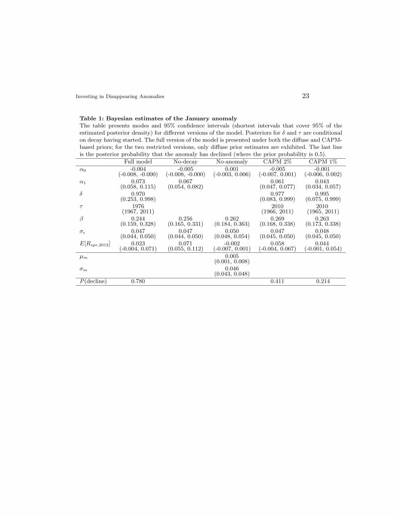
Table 1 presents the estimation results, in the form of posterior modes and 95% highestposterior density (HPD) intervals, for the full model and for the special cases of no-decay(δ = 1) and no-anomaly (α1 = 0), all under diffuse (non-informative) priors.11

For the full model, we find the posterior probability that decay has begun to be 78%.That is, there is a 22% posterior probability that the January effect remains at full strengthas of the end of our sample in 2011. The estimated decay parameter, δ, and decline startdate, τ , are 0.97 and 1976, respectively. The initial level of the anomaly, α1, is estimatedat 7.3%. Overall, the mean return for the first out-of-sample January (2012) is estimatedat 2.3%, a decline of about two-thirds from the pre-discovery level.

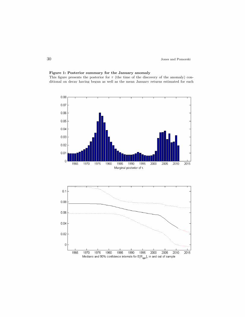
As discussed in the introduction, one advantage of the Bayesian approach is the exactfinite sample inference it offers, even for discrete parameters such as τ . This is illustratedin Figure 1, which plots the posterior distribution of τ under diffuse priors (conditionalon decay having begun). The posterior is clearly bimodal, with the primary mode in 1976and a secondary mode in the early 2000s, driven by the high January returns of 2000 and2001.

It is possible that bimodality of τ reflects “multiple discoveries” of the anomaly.12

When the anomaly is first incorporated into investors’ portfolios, it gradually declines andbecomes less attractive. Over time, investors chasing returns may focus on other strategies,consistent with work showing that portfolio managers respond to fashions (e.g., Cooper,Dimitrov, and Rau, 2001). As long as the underlying reasons for the anomaly (e.g., tax lossselling) persist, this may lead to a rebound in the anomaly’s strength, and the increasingreturns may eventually attract investors back. While the evidence we present here isconsistent with such behavior, without further data to support it this explanation is onlyspeculative.

The second panel of Figure 1 presents the evolution of the January mean return overthe sample period and the next few out-of-sample years based on the full-sample posterior.While there is a substantial amount of estimation uncertainty, a downward path is clearlyevident. The estimates are fairly constant at about 8% until the mid-1970s, when thedecline likely started, and then decrease steadily until about 2000. At that stage, past thesecond estimated peak of τ , the decline speeds up and the mean return drops to 3.4% inthe last in-sample January. The first out-of-sample mean estimate is 3.1% for January 2012(the mode of the posterior distribution is 2.3%, as reported in Table 1). Extrapolating thetrend forward, the effect would appear likely to survive for some time further.

Table 1 also presents the estimation results for the two restricted specifications, no-decay and no-anomaly. The former provides a more optimistic view of the anomaly, with

10 For δ, we use a 1000-point grid on the interval [0,1]. The grid of τ consists of allJanuaries in the sample.11 A 95% HPD is the shortest interval containing 95% of the mass of the posteriordistribution.12 We note that the modeling framework we propose here is easily extended to multiple“discovery points.”


the first out-of-sample estimate of 7.1%, more than twice above the corresponding estimatefrom the full model.

Interestingly, the no-decay estimate of the January alpha, α1, is lower than that of thefull model (6.7% versus 7.3%). This happens because the high January returns early onin the sample are averaged with the lower returns in the second half of the sample. Thispoint is worth stressing. Papers that describe a new anomaly may actually underestimateits level unless they account for its potential decline prior to their sample end. Ironically,this also means that since this lower estimate is not allowed to decay, such papers may atthe same time overestimate out-of-sample predictions.

Finally, under the no-anomaly prior the spread portfolio is allowed to exhibit a sizepremium but not a January effect. This prior leads to economically and statistically smallestimated alphas.

2.1.3 The effect of economic theory-based priors

One potential drawback of the analysis above is that it may lead (and, as we show below,indeed leads) to very large portfolio weights. Such extreme weights present an imple-mentation challenge and are perhaps economically unrealistic. Consequently, a numberof ways have been suggested to alleviate this issue. Perhaps the most straightforward isto impose ex ante constraints. A more elegant approach is to shrink optimization inputstowards values implied by economic theory and consequently tilt the implied portfoliotowards a well accepted benchmark. In the Bayesian context, one way to do so has beenproposed in Pastor and Stambaugh (1999) and Pastor (2000). They recommend that theprior for alphas (mispricing) be centered at zero, in line with a preferred asset pricingmodel, and that the strength of the belief in the model be reflected in the prior standarddeviation of alpha. Thus, we now repeat our analysis with the “2% CAPM” prior, in whichα0, α1 ∼ N(0, 0.022) and the “1% CAPM” prior, where α0, α1 ∼ N(0, 0.012).

The two rightmost columns of Table 1 present the full model estimates under theseCAPM priors. As the prior belief about α1 becomes tighter around zero, the posteriornaturally shrinks towards zero as well. This is not the only effect of imposing this view,however. Tighter priors for α0 and α1 also lead to much later estimates for τ and higherestimates for the persistence of the anomaly, δ. Consequently, the mean January returnpredicted for 2012, 5.8% for the 2% CAPM prior and 4.4% for the more conservative 1%CAPM prior, are both substantially larger than the 2.3% implied by the diffuse prior.

This effect arises because the CAPM-based priors depress the initial level of theanomaly, which must then persist for longer to be consistent with the data. Suppose,for instance, that under diffuse priors we estimate the initial level of the anomaly atα1 = 8% and the end of sample level at α1 = 3%. If the CAPM prior shrinks the initiallevel from 8% to 3%, the data will suggest that there was no decline in the sample. Thismay reduce estimates of δ so substantially as to more than offset the initial shrinkage ofα1 and lead to higher out-of-sample predictions. An implication of this result is that aprior that displays skepticism towards the initial level of anomalies and that generatesmore in-sample shrinkage may actually lead to higher return forecasts at the end of thesample.


2.2 Short-horizon autocorrelations in equity index returns

... we learned that over the past decade several investment firms – most no-tably, Morgan Stanley and D.E. Shaw – have been engaged in high-frequencyequity trading strategies specifically designed to take advantage of the kindof patterns we uncovered in 1988.

Lo and MacKinlay(1999)

While short-horizon autocorrelations in individual equity returns had been noticed asfar back as Fama (1965), the extremely high short-term autocorrelations of diversifiedequity indices were generally unknown until Lo and MacKinlay (1988).13 Their resultsimply weekly return autocorrelations as high as 15% for the value-weighted and 30%for the equally-weighted CRSP index. While not a violation of market efficiency per se,autocorrelations of this magnitude are viewed as anomalous in light of the dominant viewin the finance literature, summarized by Ahn et al. (2002), that “time variation in expectedreturns is not a high-frequency phenomenon.”

While the analysis within Lo and MacKinlay (1988) suggests that index autocorrelationsmay have begun to decline by the end of their sample, it is difficult to find more recentcomparable evidence. For example, Ahn et al. (2002) examine various US index and futuresreturns since 1982 and find daily autocorrelations ranging from -9% to +22%, albeit withlarge standard errors.

2.2.1 Modeling disappearance

As with the January effect, we model the potential disappearance of index autocorrelationsusing geometric decay. Since the anomaly affects covariances rather than means, we needto rewrite our model (2). Specifically, the market return Rt is described by

Rt − µ = ρ δ(t−τ)+

(Rt−1 − µ) + εt, (4)

where x+ = max{x, 0}.The model implies that returns display a first-order autocorrelation of ρ up until and

including date τ . After that time, the autocorrelation disappears at a rate determined byδ. The extreme values δ = 0 and δ = 1 again correspond to the cases of immediate and nodisappearance.

Initially we assume εt ∼ N(0, σ2ε ). However, in light of the well-known heteroskedasticity

of weekly market returns, we also pursue a generalization in which volatility is stochasticand returns, conditional on volatility, are distributed as student-t. As discussed in Tuand Zhou (2004), the normality approximation is substantially worse for weekly returnsthan it is for daily returns, and realistic modeling of the distribution’s tails is necessary forobtaining accurate portfolio weights. The combination of stochastic volatility and student-t errors allows for a variety of departures from normality that are well documented in theliterature. In this case, we replace the assumption that εt ∼ N(0, σ2

ε ) with εt ∼ t(0, ht, ν),where the log variance process is modeled as

lnht = a+ b lnht−1 + cRt−1 + ηt (5)

13 Interestingly, a similar finding was obtained by Hawawini (1980), but it was not theprimary focus of his paper and appears to have been generally overlooked in the academicliterature.


and ηt ∼ N(0, σ2

η

). The parameter b measures the persistence of log variance, while c

allows for the possibility of a leverage effect, or a negative correlation between returnsand volatilities. ν, the student-t degrees of freedom parameter, measures the degree ofleptokurtosis in returns conditional on volatility.

As before, we also consider restricted versions of this specification. The no-anomalymodels (one with constant, one with stochastic volatility) impose the restriction thatρ = 0 (making δ and τ irrelevant). The no-decay models set δ = 1 (making τ irrelevant).Finally, we consider an investor who believes that the date of discovery was 4/1/1988,approximately when Lo and MacKinlay (1988) was published. This investor is said tofollow a “Lo and MacKinlay” model.

We consider relatively diffuse priors on the parameters in an attempt to represent priorignorance. As before, our priors allow for a 50% probability that the anomaly has not yetbegun to disappear as of sample end (time T ). Conditional on decay having begun, theprior on δ is flat on [0, 1), and the prior on τ is uniform over the set {1, 2, ..., T}. Priorson remaining parameters are independent of δ and τ and are given by

p(µ, ρ, σε) ∝ 1/σε (6)

for the constant volatility model and by

p(µ, ρ, a, b, c, ση, ν) ∝ λ exp(−λν)/ση (7)

for the stochastic volatility model. The parameter λ is set to .05, a value that implies arelatively diffuse prior distribution for ν, with a mean of about 18 and a standard deviationof about 12.

All models are estimated using the Gibbs sampler, as before. For constant volatilityspecifications, conditional distributions are obtained for each parameter conditional on allthe rest. The conditional distributions of µ and ρ are each Gaussian, while σε is invertedgamma. The remaining parameters, δ and τ , are drawn by discretizing the parameterspace, as in Section 2.1.

Our approach to estimation of the student-t stochastic volatility model combines thealgorithms of Jacquier, Polson, and Rossi (1994) and Geweke (1993). In essence, we aug-ment observed price data with unobserved volatility data. Conditional on the augmenteddata set, estimation proceeds similarly to the above method, relying on the propertiesof the Gaussian augmented likelihood. We describe this procedure in more detail in theappendix.

2.2.2 Data

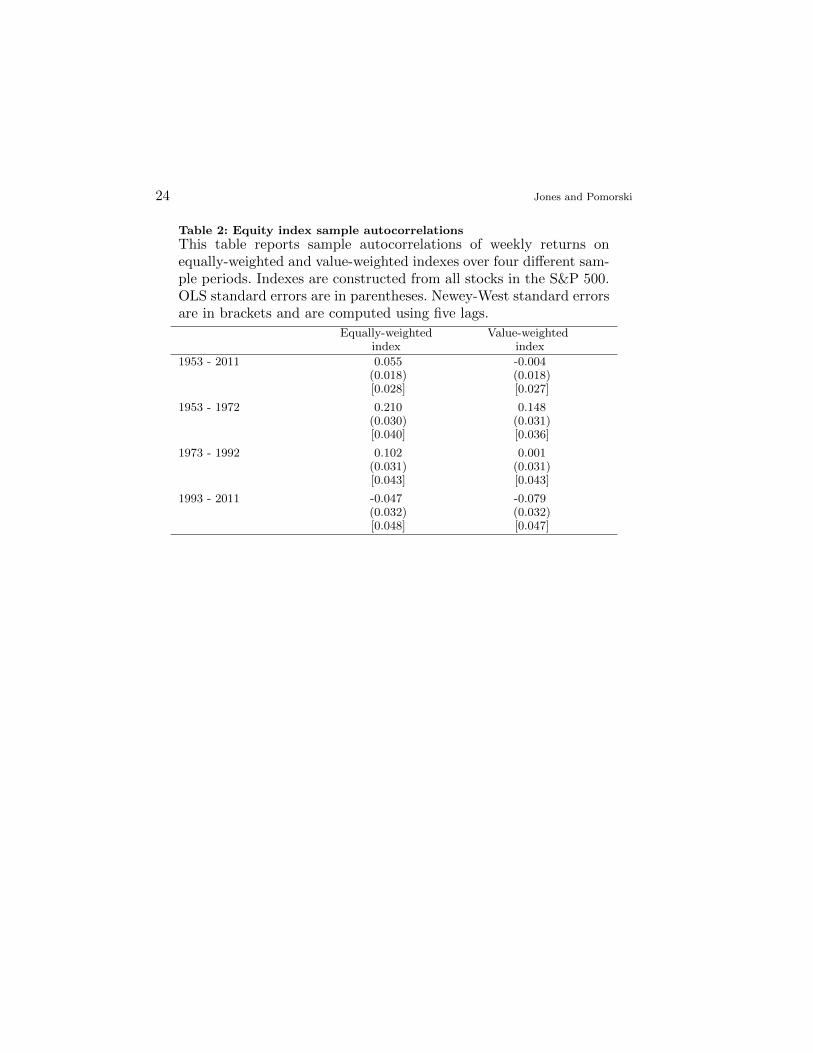
Following Lo and MacKinlay (1988), we work with weekly returns on value- and equally-weighted CRSP indexes. To minimize biases induced by nontrading and other microstruc-ture effects, we examine indexes based only on stocks in the S&P 500.14 Our sample startsin January of 1953, shortly after the end of Saturday trading on the NYSE, and ends inDecember of 2011. Weekly returns are computed by geometrically compounding daily re-turns from one Wednesday to the following Wednesday. If a Wednesday return is missing,Thursday’s return is used instead; if the Thursday return is also missing, then the Tuesdayreturn is used. The only missing week is from September 11 to 16 of 2001, when trading

14 Following Fisher (1966), Ahn et al. (2002) argue that positive index autocorrelationsmay be at least partly spurious as the result of nontrading.


was suspended due to the events of September 11. Our sample therefore consists of 3,077weeks.

Table 2 reports sample autocorrelations for our entire sample and three subsamples.For both equally-weighted (EW) and value-weighted (VW) indexes, autocorrelations arestrong in the first third of the sample period, with values of 0.21 and 0.15, respectively. Inthe middle third of the sample, the autocorrelation of the EW index is about half of itsoriginal level, while autocorrelation in the VW index has disappeared. In the final third,both indexes display slightly negative but insignificant autocorrelations.

2.2.3 Posterior summaries

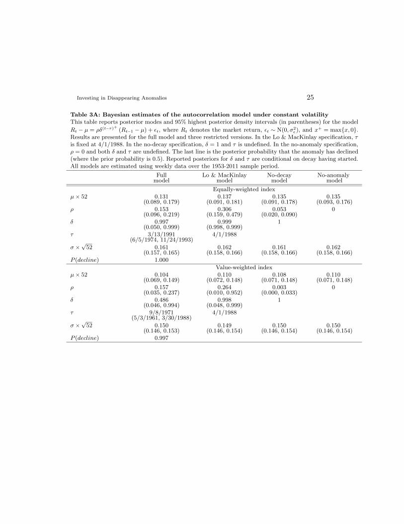
The results in Table 2 suggest that weekly autocorrelations have diminished over time.We refine this result by analyzing the model in (4) using the Bayesian methods describedabove. The posterior modes and 95% HPD intervals for the model parameters are shownin Table 3. The µ and σ parameters are annualized for easier interpretation. As before, wereport results for the δ and τ parameters for the full model conditional on decay havingbegun. For both indexes and for both volatility specifications the probability that decayhas started by the end of the sample is essentially 100%.

Panel A of Table 3 was obtained under the assumption of constant volatility. For theequally-weighted index, the mode of ρ differs significantly across specifications. It rangesfrom about 30% under the Lo and MacKinlay (LM) model to 5% under the no-decaymodel. The full model produces an intermediate but still sizable value of 15%. For boththe full and LM models, the posterior mode of δ is close to one, suggesting extremepersistence or near-zero decay. However, this parameter is inaccurately estimated for thefull model, and values close to zero are within the 95% HPD interval.

For the value-weighted index, results are somewhat different. For the full model, theposterior of δ now has a mode of 0.486 rather than 0.997, though that parameter remainsvery uncertain. The initial autocorrelation ρ is, surprisingly, about the same for the VWindex as it is for the EW index, though under the LM model it is somewhat lower. Forboth models, the posterior of ρ is much less precise for the VW index as it was for theEW index.

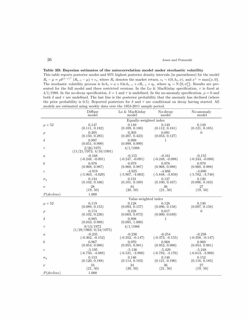
Panel B of Table 3 extends the model to the fat-tailed stochastic volatility processproposed in (5). Posteriors of the stochastic volatility parameters a, b, c, and ση are fairlytypical of those found in the literature. Values of b near one indicate that volatility ishighly persistent, while negative values of c are consistent with a leverage effect. Averagelevels of volatility, implied by a and b, are consistent with the unconditional estimatesof Panel A. The parameter ν, which represents the degrees of freedom in the student-t-distributed residual, is centered between 27 and 36, indicating that stochastic volatility isresponsible for almost all of the leptokurtosis in weekly returns.

Under stochastic volatility, the autocorrelation results for the equally-weighted indexare similar to the constant volatility case. Initial autocorrelations remain large for thefull and LM models, even for the VW index. In addition, there continues to be muchuncertainty about the decay parameter δ, particularly under for the full model and for theVW index.

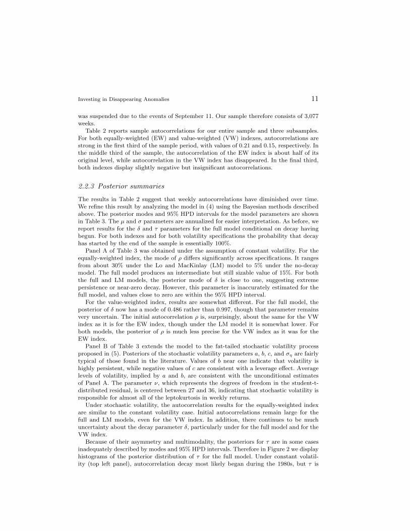
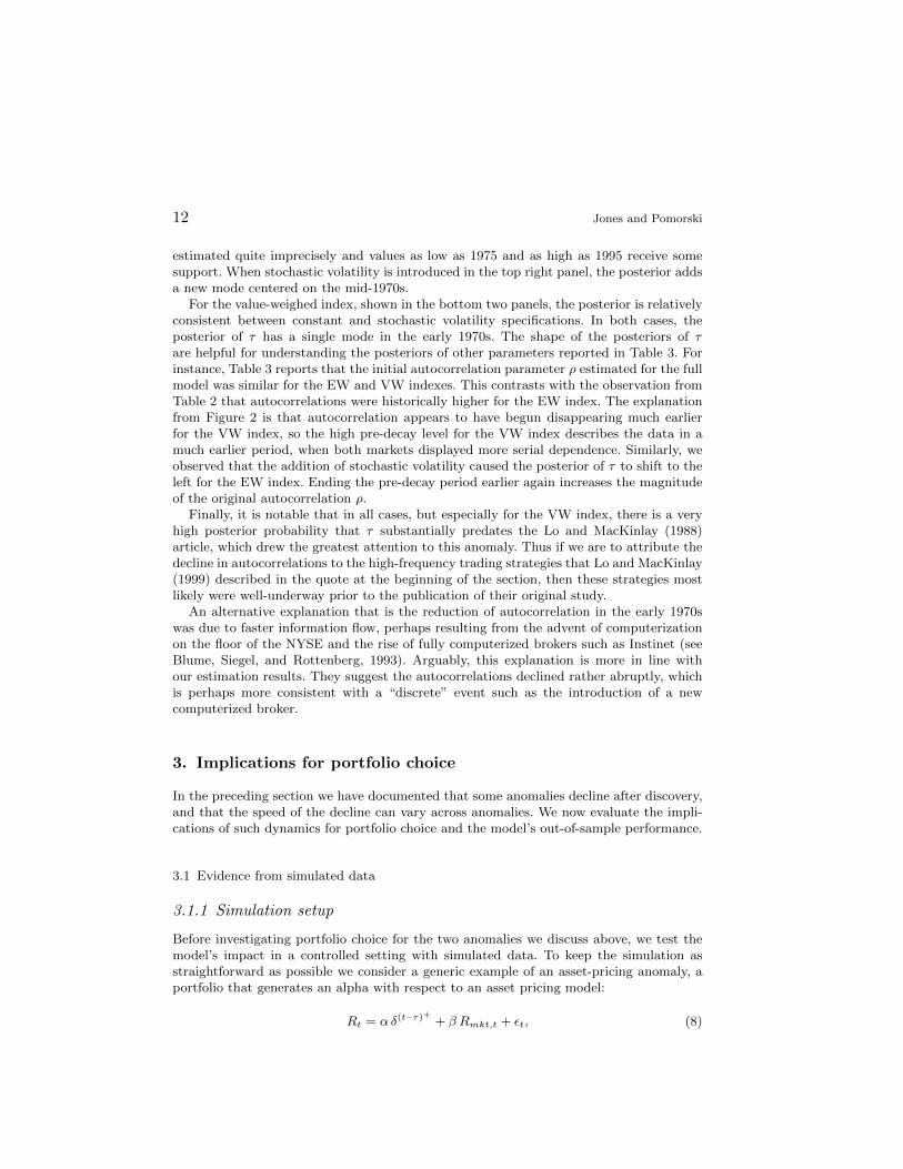
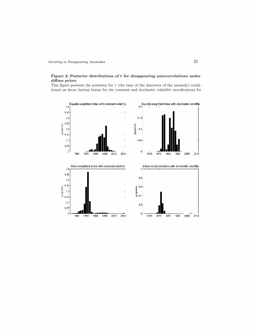
Because of their asymmetry and multimodality, the posteriors for τ are in some casesinadequately described by modes and 95% HPD intervals. Therefore in Figure 2 we displayhistograms of the posterior distribution of τ for the full model. Under constant volatil-ity (top left panel), autocorrelation decay most likely began during the 1980s, but τ is


estimated quite imprecisely and values as low as 1975 and as high as 1995 receive somesupport. When stochastic volatility is introduced in the top right panel, the posterior addsa new mode centered on the mid-1970s.

For the value-weighed index, shown in the bottom two panels, the posterior is relativelyconsistent between constant and stochastic volatility specifications. In both cases, theposterior of τ has a single mode in the early 1970s. The shape of the posteriors of τare helpful for understanding the posteriors of other parameters reported in Table 3. Forinstance, Table 3 reports that the initial autocorrelation parameter ρ estimated for the fullmodel was similar for the EW and VW indexes. This contrasts with the observation fromTable 2 that autocorrelations were historically higher for the EW index. The explanationfrom Figure 2 is that autocorrelation appears to have begun disappearing much earlierfor the VW index, so the high pre-decay level for the VW index describes the data in amuch earlier period, when both markets displayed more serial dependence. Similarly, weobserved that the addition of stochastic volatility caused the posterior of τ to shift to theleft for the EW index. Ending the pre-decay period earlier again increases the magnitudeof the original autocorrelation ρ.

Finally, it is notable that in all cases, but especially for the VW index, there is a veryhigh posterior probability that τ substantially predates the Lo and MacKinlay (1988)article, which drew the greatest attention to this anomaly. Thus if we are to attribute thedecline in autocorrelations to the high-frequency trading strategies that Lo and MacKinlay(1999) described in the quote at the beginning of the section, then these strategies mostlikely were well-underway prior to the publication of their original study.

An alternative explanation that is the reduction of autocorrelation in the early 1970swas due to faster information flow, perhaps resulting from the advent of computerizationon the floor of the NYSE and the rise of fully computerized brokers such as Instinet (seeBlume, Siegel, and Rottenberg, 1993). Arguably, this explanation is more in line withour estimation results. They suggest the autocorrelations declined rather abruptly, whichis perhaps more consistent with a “discrete” event such as the introduction of a newcomputerized broker.

3. Implications for portfolio choice

In the preceding section we have documented that some anomalies decline after discovery,and that the speed of the decline can vary across anomalies. We now evaluate the impli-cations of such dynamics for portfolio choice and the model’s out-of-sample performance.

3.1 Evidence from simulated data

3.1.1 Simulation setup

Before investigating portfolio choice for the two anomalies we discuss above, we test themodel’s impact in a controlled setting with simulated data. To keep the simulation asstraightforward as possible we consider a generic example of an asset-pricing anomaly, aportfolio that generates an alpha with respect to an asset pricing model:

Rt = αδ(t−τ)+

+ β Rmkt,t + εt, (8)


where Rt is the excess return on the anomaly portfolio, Rmkt,t ∼ N(µmkt, σ2mkt) is the

excess return on the market portfolio, εt ∼ N(0, σ2ε ), and x+ = max{x, 0}. As before, the

evolution of the anomaly is described by the triple (α, τ, δ), which captures the initial levelof the anomaly, the time that it starts to decline, and the speed of decay, respectively.

To evaluate the impact our approach has on portfolio choice, we need to translateestimation results into forward-looking predictive estimates of the mean and the varianceof anomaly returns. The anomaly portfolio’s predictive mean is computed as

µ = E [E[Rt+1|θ]] = E[αδ(t−τ+1)+ + β µmkt

], (9)

where a “tilde” denotes a moment estimated by averaging across all Gibbs draws andwhere θ denotes all parameters of the model. Predictive variances are calculated using thevariance decomposition

σ2 = E [Var(Rt+1|θ)] + Var (E[Rt+1|θ])

= E[β2σ2

mkt + σ2ε

]+ Var

(αδ(t−τ+1)+ + β µmkt

)Similar calculations produce the predictive moments of the market portfolio and the pre-dictive covariance between the two assets.

Armed with these estimates we consider a myopic Bayesian investor with quadraticutility,

µp −A

2σ2p, (10)

where µp and σp denote the predictive mean and standard deviation of the investor’sportfolio return. To keep the model simple and tractable, here and for the January effectwe consider two risky assets only, the anomaly portfolio and the market portfolio, as wellas the one-month Treasury bill. For return autocorrelations we simplify the setup to thechoice between the market portfolio (either VW or EW) and the risk-free asset. In all ourexamples, the investor’s risk aversion parameter A is set to 10. This choice implies that theinvestor who observed the entire sample of market returns would allocate approximately100% of his wealth to the market portfolio.15

Finally, based on the above inputs, we compute optimal portfolios implied by our fullmodel, which allows for anomalies’ gradual disappearance. We assess the model’s perfor-mance by comparing this portfolio to those implied by two nested versions of the model:the no-decay specification, which acknowledges the anomaly but does not allow it to dis-appear, and the no-anomaly specification, which rules out the existence of the anomaly.For each of these portfolios we compute the out-of-sample performance using a gradu-ally extending estimation window. First, we estimate the model using an initial subset ofour data. We then form portfolios that are held over the first out-of-sample period andrecord their returns. We next increase the estimation window by one period and repeatthe process, until we reach the end of our sample.

15 Note that A is just a scaling factor for the portfolio weights: as A becomes larger, theweight on the risk-free asset increases, but the composition of the risky assets portfolioremains the same.


3.1.2 Simulation results

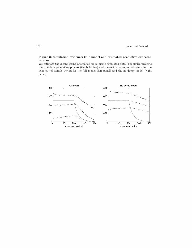
To parametrize (8) we choose α = 0.25%, β = 0, and σε = 1%, which translates into aninformation ratio of 0.25. In other words, prior to its disappearance, the anomaly is anattractive investment opportunity. We allow the investor to observe the initial 200 periodsof the anomaly’s evolution (periods -199 to 0) before making any investment. We assumethat the anomaly starts to disappear 400 periods after the start of the simulation (τ = 200)and that it decays relatively slowly, at the rate of δ = 0.975. We simulate the anomalyfor 200 periods after the start of the decay at time τ , but already 100 periods after τ theanomaly is at just 8% of its original level. The investor may also allocate funds to themarket portfolio, which has a mean return µmkt of 0.5% and a volatility σmkt of 4.5%.

We first present a summary of the estimation and the quality of out-of-sample resultsin Figure 3. The figure depicts the true alpha along with the out-of-sample predictionsgenerated by two models. The first, in the left panel, is the full specification that allowsfor decay. The second, in the right panel, is the no-decay specification that restricts δ = 1.

Not surprisingly, since we simulate the data under the null of decay, the full model doesnoticeably better in capturing the evolution of true alphas. There is, however, interestingnuance to this observation. Over the first two hundred out-of-sample periods (1-200) theanomaly does not decline. Within that subperiod the restricted model fits the data almostexactly on average. The full model, in contrast, builds in some conservatism. Since we startwith a prior that assigns 50% probability to decay and since the data do not completelydominate the prior, the posterior incorporates a significant possibility of decay and leads tothe expected returns prediction consistently below the true value. After the data generatingmodel triggers decay, starting in period τ = 200, the situation reverses. The full modelrecognizes the start of the decay and reduces the predictive mean return essentially to zeroover the subsequent 200 periods. In contrast, the no-decay approach keeps the predictivemean relatively unchanged throughout the whole period.

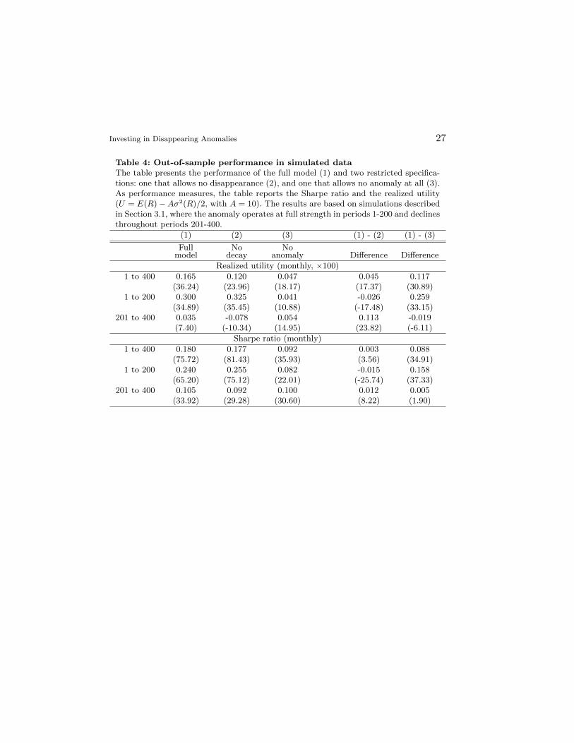
We translate the estimation output into portfolio weights and record the out-of-sampleperformance of the resulting portfolios. For completeness, we also present the performanceof the no-anomaly model, which rules out the anomaly to begin with by imposing α = 0.Table 4 summarizes the evidence for the full out-of-sample period, as well for the sub-periods before and after the start of decay. To compare the performance of the variousmodels we use two measures: the Sharpe ratio, capturing the risk-to-variability tradeoff foreach portfolio, and the realized utility measure of Fleming et al. (2001), which is simply theinvestor’s utility (10) evaluated using the sample moments of the realized out-of-sampleportfolio returns.

Over the complete out-of-sample period, the full model dominates the two restrictedspecifications. The differences are in all cases statistically significant and are particularlypronounced for realized utility. The no-decline model comes close to the full model interms of Sharpe ratio because of its aggressive allocations to the anomaly before it startsto decay. However, the tendency to be aggressive also causes the no-decay investor to takesubstantially more risk than an investor who uses the full model, especially after decayhas begun, and this leads to lower realized utility.

There are interesting patterns in the two sub-samples we consider. As expected, theno-decay model does particularly well before the anomaly starts to decline, slightly out-performing the full model but dominating the no-anomaly specification. Its performance,however, markedly decreases after decay is underway. In this period, judging by the real-ized utility, ex post the investor would have preferred not investing at all and earning no


return rather than investing using the no-decay model. The best performer in the latterperiod depends on the performance metric, with the full model having a slightly higherSharpe ratio but a slightly lower realized utility than the the no-anomaly portfolio.

These results are intuitive: if investors know that the anomaly is in full strength, theyshould allocate to it aggressively. When the anomaly starts to decay to zero, the mostconservative approach eventually becomes the most attractive. Of course, the problem isthat investors would not know in which of these two situations they find themselves, soby examining pre- and post-decay periods separately we are effectively conditioning on anunknown. It is therefore more realistic and more relevant to include both the pre-decayand post-decay regimes in the evaluation period. As we see in Table 4, in this case the fullmodel leads to better performance than the two alternatives.

3.2 Investing in January anomaly

We initiate our out-of-sample analysis of the January anomaly in December 1976, whichroughly represents the data available to an investor who read the Rozeff and Kinney(1976) article. Using this sample, we compute the implied allocation for 1977, then redothe estimation at the end of December 1977, etc. The shortest sample therefore contains15 Januaries from which the model parameters are estimated.

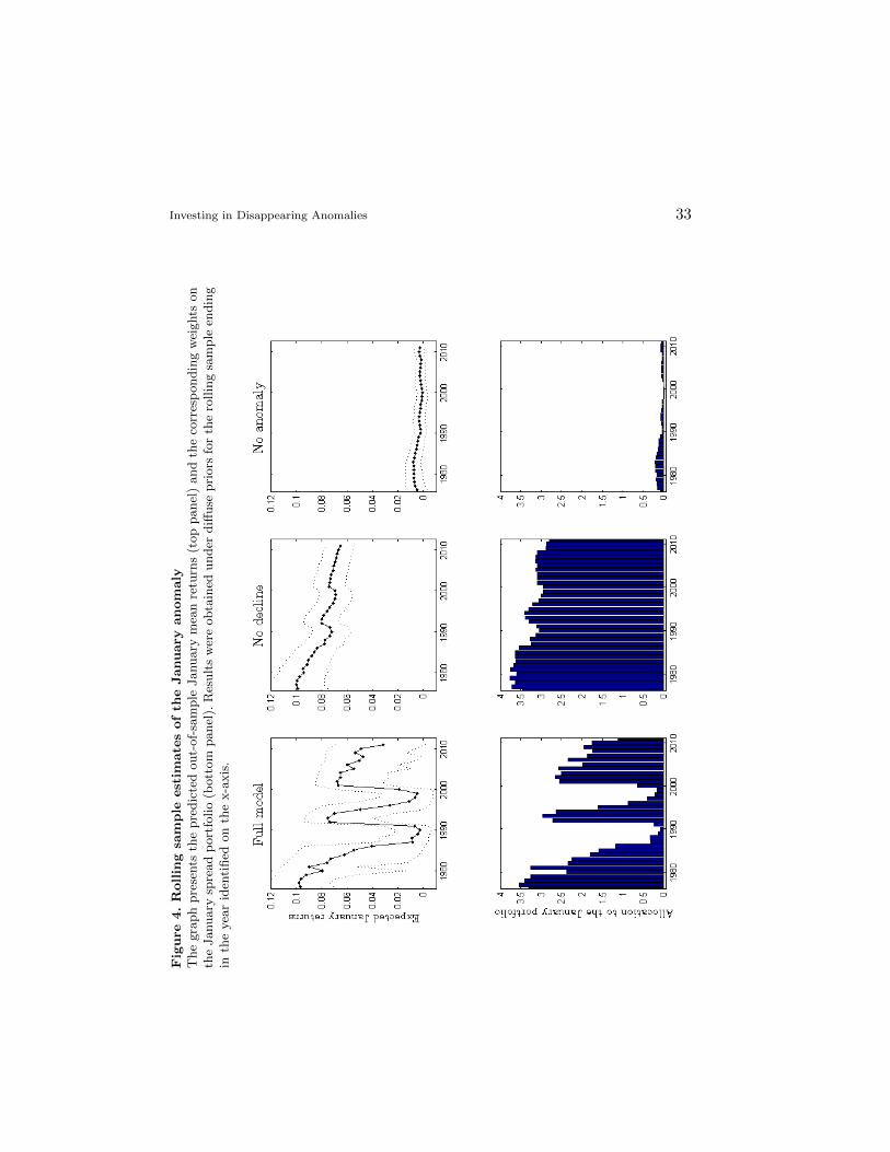
Figure 4 presents the model-implied predictive mean returns for each out-of-sampleJanuary and the corresponding January portfolio weights. As expected, the full model’sweight is between the no-decay and no-anomaly allocations. It tends to be closer to theformer early on and over time gradually approaches the latter.16 Interestingly, in the early1990s and in the early 2000s the full model dramatically increases its allocations, almostto the no-decay level. This rebound results from additional modes for τ , as we noted inSection 2.1.2, and from higher posterior mean returns in the samples ending during thoseperiods. In the full sample, the early 1990s turn out to have been less important, leavingthe posterior for τ with two clear modes (Figure 1).

A downward trend in the anomaly weights is visible for the two restricted models aswell. The no-decay investor’s January weight drops from 371% in 1977 to 280% in 2012.There is also a decline in the no-anomaly investor’s allocation, because lower Januaryreturns translate into lower α0 estimates when α1 is restricted to be zero. The no-anomalyinvestor’s weights decline from about 20% at the beginning of the sample to 5% in 2012.Note that the no-anomaly investor’s allocation can be interpreted as an allocation thataccounts for the size effect but not for the January effect.

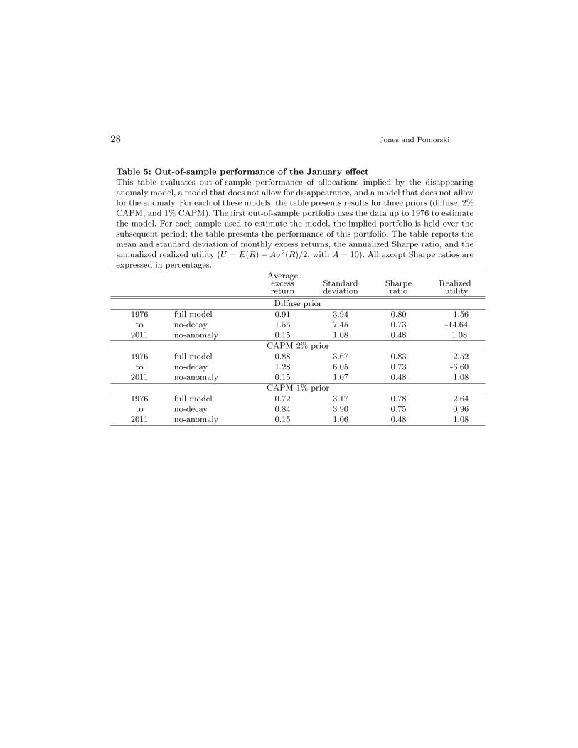
Table 5 describes the out-of-sample performance of these portfolios. Under diffuse priorson α0 and α1, the no-decay portfolio generated the highest average excess returns, 1.56%per month, as compared to 0.91% for the full model and 0.15% for the no-anomaly alloca-tion. However, this performance comes at the cost of very high risk: the no-decay standarddeviation was 7.45%, almost twice the standard deviation of the full model, 3.94%. Con-sequently, it is the full model that earns the highest out-of-sample Sharpe ratio, 0.80, andthe highest realized utility, 0.13% (1.56% using annualized average returns and standard

16 When one invokes trading costs, obviously high in the case of the spread portfolio,the allocation may well remain substantial. Assuming the round trip transaction costsof 2%, the full model allocates 42% to the January portfolio at the end of the sample,economically large but perhaps more realistic. The no-decay allocation declines to 198%and thus is still economically rather implausible.


deviation). The Sharpe ratio of the no-decay model is lower, at 0.73, and the excessiverisk of that strategy results in a negative utility, indicating a portfolio that is worse (inutility terms) than Treasury bills. The no-anomaly portfolio offers both a lower Sharperatio and a lower (but positive) realized utility.17

Table 5 also documents the performance of investors guided by our two CAPM-basedpriors on α0 and α1. As in the diffuse prior case, we observe better out-of-sample per-formance of the full model over the no-decay and no-anomaly specifications under thesetheory-based priors. The 2% CAPM (1% CAPM) Sharpe ratios of the full model and no-decay specifications are 0.83 and 0.73 (0.78 and 0.75), respectively. For both CAPM priors,the realized utility measure strongly favors the full model. Comparing full model resultsunder CAPM to those under diffuse priors, we see that CAPM priors generally improveperformance. This is consistent with the notion that shrinkage has the biggest potentialbenefits when sample sizes are small, and that the shrinkage introduced by CAPM-basedpriors is complementary to that induced by our modeling of decay.

3.3 Investing in index autocorrelations

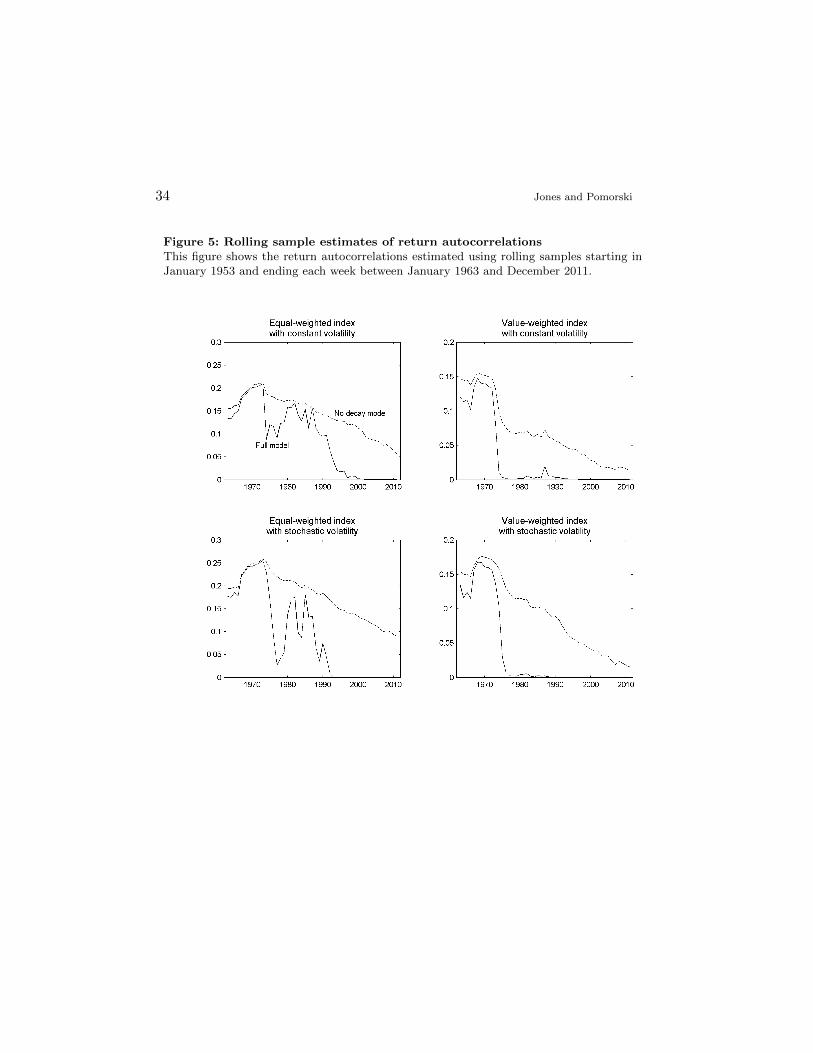
For the market index autocorrelations, we re-estimate each model using samples startingin January 1953 and ending in each week between January 1963 and December 2011.We start by plotting, in Figure 5, the rolling sample posterior means of the terminalautocorrelations ρδ(T−τ)

+, where T is the last observation of each rolling sample period.

These are the autocorrelations that an investor might have predicted, at least in the veryshort term, under each model. For visual clarity, we only plot end-of-year values. Since theno-anomaly model sets autocorrelations equal to zero, there are only two lines per panelin Figure 5.

Through the mid-1970s, the full and no-decay models are in rough agreement on thelevel of return autocorrelation, both for the EW and VW indexes, and both for the constantand stochastic volatility models. Afterward, autocorrelations drop quickly under the fullmodel (the solid line). The mid-1970s therefore appears to provide the first substantialevidence that the anomaly is disappearing. For the EW index, the mean autocorrelationunder the full model recovers somewhat during the early to mid-1980s before trending tozero over the subsequent 5-10 years. For the VW index, the mean autocorrelation dropsclose to zero well before 1980.

In contrast, under the no-decay model (the dashed line), autocorrelations are onlygradually trending downward after their peak in the 1970s. The decline becomes moreapparent as the post-discovery period becomes a more important part of the rolling sample.Nonetheless, the no-decay model still implies a substantial level of autocorrelation in theEW index by the end of our sample in 2011. For the VW index, the autocorrelation in2011 is smaller but clearly positive.

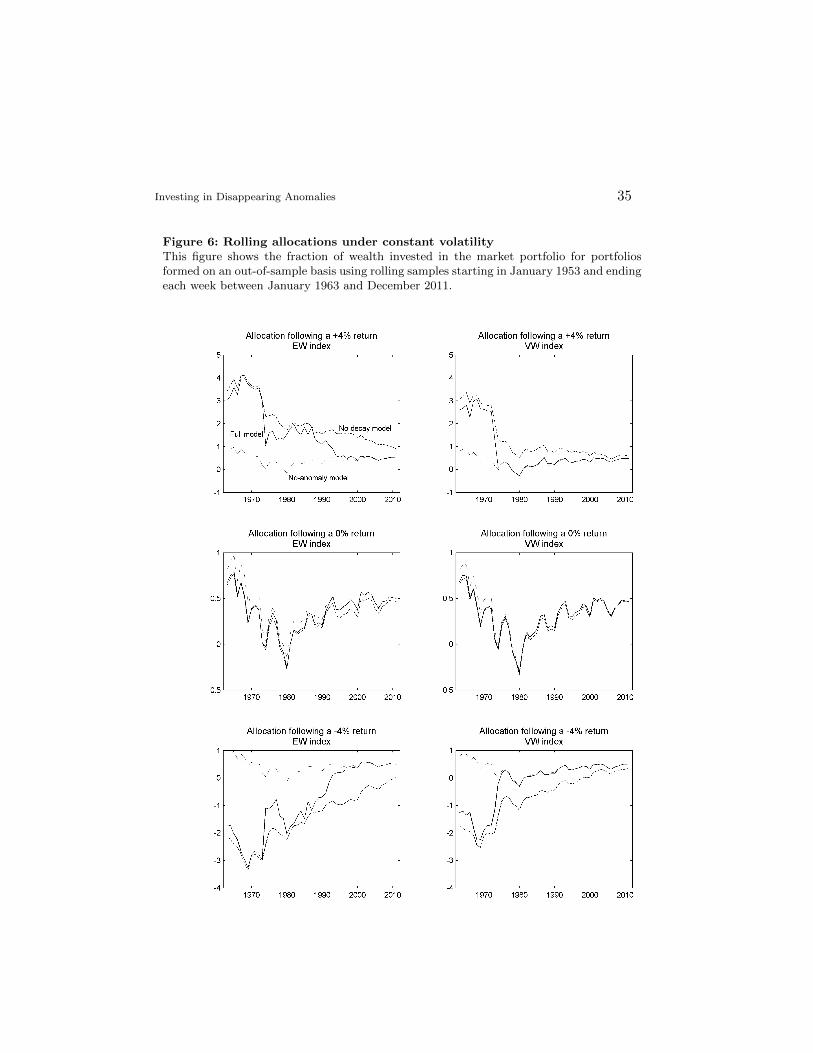
The portfolio allocations implied by the different models are shown in Figure 6. Weplot these results only for the constant volatility model. Stochastic volatility introducessubstantial variation in allocations that is unrelated to the conditional mean we are fo-cusing on, making it more difficult to interpret the allocations. They are consistent withthe conclusions we draw from the constant volatility case, however.

17 In untabulated tests, available by request, we divide the 36 years of our out-of-sampleevidence into three equal-length sub-periods and show that the full model outperformsalso in subsamples.


The panels in Figure 6 report hypothetical year-end allocations under three models forboth the EW and VW indexes. Allocations are based on the one-week ahead predictivedistribution of returns computed on a rolling sample basis. They are hypothetical in thatthe conditional mean forecast is based on one of three hypothetical values of RT ratherthan the actual value. The distribution of the parameters, however, is derived from theinvestor’s posterior distribution given actual data.

In short, the results in Figure 6 are straightforward given the autocorrelations fromFigure 5. In the early part of the sample, the investor who follows the full model choosesportfolio allocations that are fairly consistent with those of the no-decay investor. By theend of the sample, however, the investor who uses the full model is mirroring the investorwith a fixed autocorrelation of zero and investing approximately 50% in the EW or VWmarket index regardless of the past return. The transition of the full model investor isrelatively prolonged for the EW index, with a period of about 20 years during which theallocations are between those of the no-decline and no-anomaly investors. For the VWindex, the transition is much quicker and follows the patterns in Figure 5.

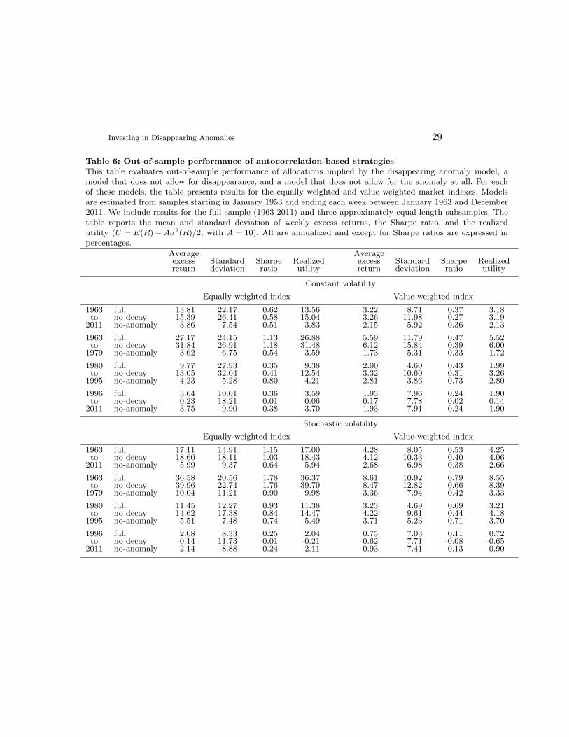
Table 6 summarizes the out of sample performance of these strategies. Under constantvolatility, the strategy based on the full model fares best in terms of its Sharpe ratio.Realized utility, however, is lower than for the no-anomaly investor. The reason for thisdiscrepancy is the misspecification represented by constant volatility. An investor whoinfers a substantial amount of autocorrelation will take a very significant position followinga large positive or negative return. When a significant position is taken during a periodof high volatility, an investor who treats volatility as constant runs the risk of earningan extremely negative return. For investors allocating to the EW index, these extremereturns were as low as -60% in a single week. Even a small number of these returns has alarge negative impact on the realized utility measure.

Results under stochastic volatility, presented in the bottom panel, are much better.Aside from the last subsample, stochastic volatility-based strategies perform much betterthan constant volatility strategies, both for the EW and VW indexes. In addition, realizedutilities for the full and no-decay models are much higher. This can be attributed to adramatic reduction in extreme negative returns, the worst of which were -17% for the fullmodel and -18% for the no-decay model.

Using stochastic volatility, the full model trounces the other specifications in terms ofboth Sharpe ratios and realized utilities. In the early subsample, its performance matchesor slightly outperforms the no-decay strategy, as both take advantage of the strong auto-correlations observed during that period. In the late subsample, its performance matchesthe conservative no-anomaly strategy, while the no-decay portfolio performs badly as ittrades on nonexistent autocorrelation.18 As in Johannes et al. (2014), who consider theout-of-sample performance of a Bayesian investor in a much different setting, it appearsthat the full benefits of return predictability can only be gained under an appropriatemodel of conditional variance.

Overall, results are very positive for the full model, supporting the conclusion thatmodeling disappearance of the anomaly is crucial.

18 As an additional robustness check, we also combine the expected return forecasts ofthe constant volatility model with the out-of-sample volatility forecast of a GARCH(1,1)fitted to the same sequence of subsamples. These results are very similar to those of themodel with stochastic volatility.


4. Conclusions

We argue that when studying anomalies or their impact on portfolio choice, it is importantto allow for the possibility of a prolonged decay. Such a decay may arise because investorsneed time to build models and capabilities or to market the idea to raise funds. Therecould also be implementation frictions, e.g., transaction costs that only slowly decreaseover time. Moreover, the market’s efficiency may itself vary over time, as suggested by Lo(2004) and Akbas et al. (2015), which will make some anomalies longer lived than others.

We propose a framework for modeling anomalies that specifically allows for a gradualdisappearance. Rather than describe an anomaly with a single parameter (e.g., its alpha),this framework calls for a triple of parameters: the initial strength (α), the time of discovery(τ), and the speed of disappearance (δ). Our approach nests and thus allows for direct testsof various economically-motivated special cases: immediate disappearance, no decline, etc.We argue that estimating this model, or an equivalent model that allows for decay, wouldbe a valuable part of any paper that identifies a new anomaly or that documents anexisting anomaly in a different market or context. The model would allow the authorsto better estimate the original full strength of the anomaly (which would be understatedif the anomaly already started declining) and would improve out-of-sample predictions(which would be overstated if the decline already began).

To illustrate the value of our approach we specialize the model to two well-knownanomalies: the January effect and short-term autocorrelations of market returns. We showthat the January effect is slowly dissipating, with the current magnitude of about a thirdof its original level. The decay likely started during the 1970s, with 1976 being the mostprobable first year of decline. We also find strong evidence for disappearance for theautocorrelations anomaly. Specifically, autocorrelations in the value-weighted index havealmost certainly declined to zero. Although there is some uncertainty about when thisdecline began, the early 1970s appear most probable, and point estimates suggest thedisappearance was quite abrupt. The autocorrelations in the equal-weighted index havedecayed more slowly, but they too have disappeared by about 1990s.

Our results shed light on how likely various explanations of the two anomalies are.The fact that both show gradual decline makes it unlikely that they were simply a resultof data mining. Their decline also suggests that they are unlikely to be risk-driven – atleast, such an explanation would need to explain why the compensation for risk decreasedslowly over time. We believe that the most probable explanation is that both the Januaryeffect and autocorrelated market returns represented genuine mispricing that was initiallyunnoticed by investors.

Moreover, our approach sheds light on what may have triggered the decay of the anoma-lies. The most likely starting year for the decline of the January anomaly is 1976, coincidingwith the publication of Rozeff and Kinney’s 1976 study. To the best of our knowledge,Rozeff and Kinney (1976) is the first paper to document January seasonalities in the stockmarket, which suggests that academic research may play a role in eliminating market inef-ficiencies. In contrast, it appears that the decay of the stock index autocorrelations beganwell ahead of the publication of Lo and MacKinlay (1988), the seminal academic articleon the subject. Instead, the timing coincides with the introduction of computerization tothe NYSE in the early 1970s, suggesting that the anomaly was sustained by the frictionsto trading, lessened in the early 1970s. This has important implications for research on theanomaly’s underlying causes. Most obviously, studies using shorter, more recent sampleperiods may provide little insight on the historical factors that contributed to the anoma-


lous behavior. For example, Ahn et al. (2002) attempt to determine the source of indexautocorrelation by examining a variety of value-weighted indexes and their correspondingfutures contracts. However, equity index futures were not traded until the 1980s or later,by which time value-weighted (though not equally-weighted) autocorrelations remained atjust a tiny fraction of their original levels.

An additional contribution is to document a surprising result that shrinking ananomaly’s returns towards a benchmark (in our case, the CAPM) may lead to increasedallocations to the anomalous asset. Such shrinkage is often proposed to alleviate the issueof large weights implied by optimizers. However, a prior that reduces the initial level ofan anomaly can cause that anomaly to persist for longer, and the higher estimated persis-tence may lead to higher end- and out-of-sample levels of the anomaly. Hence, skepticismabout the existence of tradeable inefficiencies might be better represented as a belief bothabout the levels of anomalies and their rates of disappearance. We believe that this point,not yet made in the literature, will be of interest to both academics and practitioners.

Finally, we show that accounting for decay has a substantial impact on portfolio choiceand, most importantly, that using a model that incorporates decay results in superior out-of-sample portfolio performance. This is notable, as the return predictability literaturehas recently been called into question by Goyal and Welch (2008), albeit in a differentsetting, for its inability to provide useful forecasts on an out-of-sample basis. The implicitassumption in Goyal and Welch (2008) is that the return generating process is stationary,so that the predictive relationships are unchanged over time. This “no-decay” approachoften proves problematic in the settings that we analyze as well, in many cases underper-forming strategies that ignore the abnormal return opportunities completely. However, byallowing anomalous returns to shrink over time, we are able to take advantage of returnpredictability in a way that is both conservative and adaptive. Our results suggest thatpredictive return models may be an important component of active investment strategiesonce those models allow for the possibility of decay.

1. Student-t / stochastic volatility sampling algorithm

In this appendix we adapt the methods of Geweke (1993) and Jacquier, Polson, and Rossi(1994, hereafter JPR) to estimate the stochastic volatility model

Rt − µ = ρδ(t−τ)+

(Rt−1 − µ) + εt (A1)

lnht = a+ b lnht−1 + cRt−1 + ηt, (A2)

where εt ∼ t(0, ht, ν), ηt ∼ N(0, σ2

η

), and t ∈ {1, 2, ..., T}.

Following Geweke (1993), assuming that εt ∼ t(0, ht, ν) is equivalent to assuming thatεt =

√ht√ωtε

∗t, where ε∗t is a standard normal and ν/ωt ∼ χ2(ν). We adopt this latter

representation.Introducing stochastic volatility to the framework outlined in Section 2.2 requires

adding an additional component to the Gibbs sampling algorithm. First, conditioningon the time series of ht and of ωt, we draw the parameters ση, a, b, c, and ν. Second,conditional on all the parameters as well as the asset returns, we draw values of ht andωt.

Conditional on the ht, drawing the parameters ση, a, b, and c uses standard regressionresults such as those found in Zellner (1971). In particular, the distribution of ση is an


inverted gamma, and the vector [a, b, c] given ση is multivariate normal. Conditional onthe ωt, drawing ν is also fairly straightforward. Following Geweke (1993), the conditionaldensity of νt is

(ν/2)Tν/2Γ(ν/2) exp(−ξν), where ξ =1

2

T∑t=1

[ln(ωt) + ω−1t

]+ λ. (A3)

We sample from this univariate density using the griddy Gibbs sampler. To draw thelatent variable ωt given all the parameter values and the time series of ht and Rt, we usethe result from Geweke that (

ε2t + ν)/ωt ∼ χ2(ν + 1). (A4)

The last step is to draw the ht conditional on the model parameters and the ωt. As inJPR, we draw the entire time series of ht by cycling through each element one at a time.In effect, this step actually consists of T separate draws from the densities

p(ht|h1, h2, ..., ht−1, ht+1, ..., hT , R1, R2, ..., RT , ω1, ω2, ..., ωT , θ), (A5)

where θ represents the vector of all model parameters. Similar to JPR, the Markoviannature of the ht process and Bayes rule together imply that this density is proportionalto

p(ht|ht−1, θ)p(ht+1|ht)p(Rt|ht, ωt). (A6)

Furthermore, this product of densities is proportional to

f(ht) ≡1

htexp

(− (lnht −mt)

2

2s2t

)1√ht

exp

(− ε2t

2ωtht

), (A7)

where

εt = (Rt − µ)− ρδ(t−τ)+(Rt−1 − µ) (A8)

mt = [a(1− b) + b(lnht−1 + lnht+1) + cRt−1 − bcRt] /(1 + b2) (A9)

s2 = σ2η/(1 + b2) (A10)

When c = 0 and ωt = 1, these match the formulas found in JPR. Similarly to JPR, we usethe Metropolis Hastings algorithm with the candidate generating density

q(ht) ∝ h−(φ+1)t exp(−ψt/ht), (A11)

where φ = −1.5 + (1− 2 exp(s2))/(1− exp(s2)) and ψt = .5ε2/ωt + (φ+ 1) exp(mt +.5s2). This produces a inverse gamma candidate generating density that approximatesthe target density in (A7). JPR show that this candidate generator has relatively thicktails and demonstrates good convergence properties.

A candidate draw h∗t from this inverse gamma is then accepted, replacing the currentdraw ht, with probability

min

{f(h∗t)/q(h

∗t)

f(ht)/q(ht), 1

}(A12)

If the draw is rejected, the current draw ht is kept.By drawing each ht in turn, from t = 1 to t = T , a new draw of the time series of ht is

obtained. While the algorithm must be modified for t = 1 and t = T , this is straightforwardfollowing the procedure of Jacquier, Polson, and Rossi (2001).


References

Ahn, D., Boudoukh, J., Richardson, M. and Whitelaw, R.F. (2002) Partial adjustmentor stale prices? Implications from stock index and futures return autocorrelations,Review of Financial Studies 15, 655-689.

Akbas, F., Armstrong, W.J., Sorescu, S. and Subrahmanyam, A. (2015) Capital mar-ket efficiency and arbitrage efficacy, Journal of Financial and Quantitative Analysis,forthcoming.

Avramov, D. (2004) Stock return predictability and asset pricing models, Review of Fi-nancial Studies 17, 699-738.

Banz, R.W. (1981) The relationship between return and market value of common stocks,Journal of Financial Economics 9, 3-18.

Blume, M.E., Siegel, J.J. and Rottenberg, D. (1993) Revolution on Wall Street: The Riseand Decline of the New York Stock Exchange, W.W. Norton, New York, NY.

Busse, J. and Irvine, P. (2006) Bayesian alphas and mutual fund persistence, Journal OfFinance 61, 2251-2288.

Conrad, J. and Kaul, G. (1988) Time-variation in expected returns, Journal of Business61, 409-425.

Cooper, M.J., Dimitrov, O. and Rau, P.R. (2001) A Rose.com by any other name, Journalof Finance 56, 2371-2388.

Fama, E. (1965) The behavior of stock prices, Journal of Business 38, 34-105.Fisher, L. (1966) Some new stock market indexes, Journal of Business 39, 191-225.Fleming, J., Kirby, C. and Ostdiek, B. (2001) The economic value of volatility timing,

Journal of Finance 56, 329-352.Geman, S. and Geman, D. (1984) Stochastic relaxation, Gibbs distributions, and the

Bayesian restoration of images, IEEE Transactions on Pattern Analysis and MachineIntelligence 6, 721-741.

Geweke, J. (1993) Bayesian treatment of the independent student-t linear model, Journalof Applied Econometrics 8, S19-S40.

Goyal, A. and Welch, I. (2008) A comprehensive look at the empirical performance ofequity premium prediction, Review of Financial Studies 21, 1455-1508.

Hand, J., Green, G. and Soliman, M. (2011) Going, going, gone? The demise of the accrualsanomaly, Management Science 57, 797-816.

Haugen, R.A. and Jorion, P. (1996) The January effect: Still there after all these years,Financial Analysts Journal, January-February, 27-31.

Hawawini, G. (1980) Intertemporal cross dependence in securities daily returns and theshort-term intervailing effect on systematic risk, Journal of Financial and QuantitativeAnalysis 15, 139-149.

Jacquier, E., Polson, N.G. and Rossi, P.E. (1994) Bayesian analysis of stochastic volatilitymodels, Journal of Business and Economic Statistics 12, 371-389.

Jegadeesh N. and Titman, S. (2001) Profitability of momentum strategies: An evaluationof alternative explanations, Journal of Finance 56, 699-720.

Johannes, M., Korteweg, A. and Polson, N.G. (2014) Sequential learning, predictive re-gressions and optimal portfolios, Journal of Finance 69, 611-644.

Jones, C. and Shanken, J. (2005) Mutual fund performance with learning across funds,Journal of Financial Economics 78, 507-552.

Jorion, P. (1986) Bayes-Stein estimation for portfolio analysis, Journal of Financial andQuantitative Analysis 21, 279-292.


Kandel, S. and Stambaugh, R.F. (1996) On the predictability of stock returns: An AssetAllocation Perspective, Journal of Finance 51, 385-424.

Keim, D.B. (1983) Size-related anomalies and stock return seasonality: Further empiricalevidence, Journal of Financial Economics 12, 13-32.

Lo, A.W. (2004) The Adaptive market hypothesis: Market efficiency from an evolutionaryperspective, Journal of Portfolio Management 30, 15-29.

Lo, A.W. and MacKinlay, A.C. (1988) Stock market prices do not follow random walks:Evidence from a simple specification test, Review of Financial Studies 1, 41-66.

Lo, A.W. and MacKinlay, A.C. (1999) A Non-Random Walk Down Wall Street, PrincetonUniversity Press, Princeton, NJ.

McLean, R.D. and Pontiff, J. (2015) Does academic research destroy stock return pre-dictability?, Journal of Finance, forthcoming.

McQueen, G. and Thorley, S. (1997) Do investors learn? Evidence from a gold marketanomaly, Financial Review 32, 501-525.

Mittoo, U. and Thompson, R. (1990) Do the capital markets learn from financialeconomists?, working paper, University of Manitoba.

Pastor, L. (2000) Portfolio selection and asset pricing models, Journal of Finance 40,179-223.

Pastor, L. and Stambaugh, R.F. (1999) Cost of equity capital and model mispricing,Journal of Finance 54, 67-121.

Pastor, L. and Stambaugh, R.F. (2001) The equity premium and structural breaks, Journalof Finance 56, 1207-1239.

Pastor, L. and Stambaugh, R.F. (2002) Mutual fund performance and seemingly unrelatedassets, Journal of Financial Economics 63, 315-349.

Reinganum, M.R. (1983) The anomalous stock market behavior of small firms in January:Empirical tests for tax-loss selling effects, Journal of Financial Economics 12, 89-104.

Rozeff, M. and Kinney, W. (1976) Capital market seasonality: The case of stock returns,Journal of Financial Economics 3, 379-402.

Schwert, G.W. (2003) Anomalies and market efficiency, in: G. Constantinides, M. Har-ris, and R.M. Stulz (eds.), Handbook of the Economics of Finance, North-Holland,Amsterdam, 937-972.

Sloan, R. (1996) Do stock prices fully reflect information in accruals and cash flows aboutfuture earnings, The Accounting Review 71, 289-316.

Tu, J. and Zhou, G. (2004) Data-generating process uncertainty: What difference does itmake in portfolio decisions? Journal of Financial Economics 72, 385-421.

Tu, J. and Zhou, G. (2010) Incorporating economic objectives into Bayesian priors: Port-folio choice under parameter uncertainty, Journal of Financial and Quantitative Anal-ysis 45, 959-986.

Watts, R. (1978) Systematic ‘abnormal’ returns after quarterly earnings announcements,Journal of Financial Economics 6, 127-150.

Zellner, A. (1971) An Introduction to Bayesian Inference in Econometrics, Wiley, NewYork, NY.


Table 1: Bayesian estimates of the January anomalyThe table presents modes and 95% confidence intervals (shortest intervals that cover 95% of theestimated posterior density) for different versions of the model. Posteriors for δ and τ are conditionalon decay having started. The full version of the model is presented under both the diffuse and CAPM-based priors; for the two restricted versions, only diffuse prior estimates are exhibited. The last lineis the posterior probability that the anomaly has declined (where the prior probability is 0.5).

Full model No-decay No-anomaly CAPM 2% CAPM 1%

α0 -0.004 -0.005 0.001 -0.005 -0.001(-0.008, -0.000) (-0.008, -0.000) (-0.003, 0.006) (-0.007, 0.001) (-0.006, 0.002)

α1 0.073 0.067 0.061 0.043(0.058, 0.115) (0.054, 0.082) (0.047, 0.077) (0.034, 0.057)

δ 0.970 0.977 0.995(0.253, 0.998) (0.083, 0.999) (0.075, 0.999)

τ 1976 2010 2010(1967, 2011) (1966, 2011) (1965, 2011)

β 0.244 0.256 0.262 0.269 0.263(0.159, 0.328) (0.165, 0.331) (0.184, 0.363) (0.168, 0.338) (0.173, 0.338)

σε 0.047 0.047 0.050 0.047 0.048(0.044, 0.050) (0.044, 0.050) (0.048, 0.054) (0.045, 0.050) (0.045, 0.050)

E[Rspr,2012] 0.023 0.071 -0.002 0.058 0.044(-0.004, 0.071) (0.055, 0.112) (-0.007, 0.001) (-0.004, 0.067) (-0.001, 0.054)

µm 0.005(0.001, 0.008)

σm 0.046(0.043, 0.048)

P (decline) 0.780 0.411 0.214


Table 2: Equity index sample autocorrelationsThis table reports sample autocorrelations of weekly returns onequally-weighted and value-weighted indexes over four different sam-ple periods. Indexes are constructed from all stocks in the S&P 500.OLS standard errors are in parentheses. Newey-West standard errorsare in brackets and are computed using five lags.

Equally-weighted Value-weightedindex index

1953 - 2011 0.055 -0.004(0.018) (0.018)[0.028] [0.027]

1953 - 1972 0.210 0.148(0.030) (0.031)[0.040] [0.036]

1973 - 1992 0.102 0.001(0.031) (0.031)[0.043] [0.043]

1993 - 2011 -0.047 -0.079(0.032) (0.032)[0.048] [0.047]


Table 3A: Bayesian estimates of the autocorrelation model under constant volatilityThis table reports posterior modes and 95% highest posterior density intervals (in parentheses) for the model


(Rt−1 − µ) + εt, where Rt denotes the market return, εt ∼ N(0, σ2ε ), and x+ = max{x, 0}.

Results are presented for the full model and three restricted versions. In the Lo & MacKinlay specification, τis fixed at 4/1/1988. In the no-decay specification, δ = 1 and τ is undefined. In the no-anomaly specification,ρ = 0 and both δ and τ are undefined. The last line is the posterior probability that the anomaly has declined(where the prior probability is 0.5). Reported posteriors for δ and τ are conditional on decay having started.All models are estimated using weekly data over the 1953-2011 sample period.

Full Lo & MacKinlay No-decay No-anomalymodel model model model

Equally-weighted indexµ× 52 0.131 0.137 0.135 0.135

(0.089, 0.179) (0.091, 0.181) (0.091, 0.178) (0.093, 0.176)ρ 0.153 0.306 0.053 0

(0.096, 0.219) (0.159, 0.479) (0.020, 0.090)δ 0.997 0.999 1

(0.050, 0.999) (0.998, 0.999)τ 3/13/1991 4/1/1988

(6/5/1974, 11/24/1993)

σ ×√

52 0.161 0.162 0.161 0.162(0.157, 0.165) (0.158, 0.166) (0.158, 0.166) (0.158, 0.166)

P (decline) 1.000

Value-weighted indexµ× 52 0.104 0.110 0.108 0.110

(0.069, 0.149) (0.072, 0.148) (0.071, 0.148) (0.071, 0.148)ρ 0.157 0.264 0.003 0

(0.035, 0.237) (0.010, 0.952) (0.000, 0.033)δ 0.486 0.998 1

(0.046, 0.994) (0.048, 0.999)τ 9/8/1971 4/1/1988

(5/3/1961, 3/30/1988)

σ ×√

52 0.150 0.149 0.150 0.150(0.146, 0.153) (0.146, 0.154) (0.146, 0.154) (0.146, 0.154)

P (decline) 0.997


Table 3B: Bayesian estimates of the autocorrelation model under stochastic volatilityThis table reports posterior modes and 95% highest posterior density intervals (in parentheses) for the model


(Rt−1 − µ) + εt, where Rt denotes the market return, εt ∼ t(0, ht, ν), and x+ = max{x, 0}.The stochastic volatility process is lnht = a+ b lnht−1 + cRt−1 + ηt, where ηt ∼ N

(0, σ2

η

). Results are pre-

sented for the full model and three restricted versions. In the Lo & MacKinlay specification, τ is fixed at4/1/1988. In the no-decay specification, δ = 1 and τ is undefined. In the no-anomaly specification, ρ = 0 andboth δ and τ are undefined. The last line is the posterior probability that the anomaly has declined (wherethe prior probability is 0.5). Reported posteriors for δ and τ are conditional on decay having started. Allmodels are estimated using weekly data over the 1953-2011 sample period.

Diffuse Lo & MacKinlay No-decay No-anomalymodel model model model

Equally-weighted indexµ× 52 0.147 0.149 0.149 0.149

(0.111, 0.182) (0.109, 0.180) (0.112, 0.181) (0.121, 0.185)ρ 0.205 0.303 0.091 0

(0.150, 0.285) (0.207, 0.423) (0.053, 0.127)δ 0.997 0.999 1

(0.051, 0.999) (0.999, 0.999)τ 2/26/1975 4/1/1988

(11/21/1973, 4/10/1991)a -0.168 -0.155 -0.161 -0.155

(-0.248, -0.091) (-0.247, -0.091) (-0.248, -0.088) (-0.243, -0.088)b 0.978 0.979 0.978 0.979

(0.968, 0.987) (0.968, 0.987) (0.968, 0.988) (0.968, 0.988)c -4.919 -4.925 -4.866 -4.690

(-5.963, -4.029) (-5.907, -4.003) (-5.848, -3.859) (-5.782, -3.748)ση 0.134 0.131 0.127 0.120

(0.102, 0.166) (0.101, 0.169) (0.100, 0.167) (0.096, 0.163)ν 28 34 36 27

(19, 50) (20, 50) (21, 50) (19, 50)P (decline) 1.000

Value-weighted indexµ× 52 0.119 0.128 0.128 0.130

(0.089, 0.155) (0.093, 0.157) (0.096, 0.158) (0.097, 0.158)ρ 0.174 0.228 0.017 0

(0.102, 0.236) (0.003, 0.873) (0.000, 0.049)δ 0.985 0.998 1

(0.043, 0.988) (0.095, 1.000)τ 9/13/1972 4/1/1988

(1/29/1969, 9/24/1975)a -0.235 -0.236 -0.254 -0.238

(-0.362, -0.152) (-0.352, -0.147) (-0.373, -0.155) (-0.358, -0.147)b 0.967 0.970 0.968 0.969

(0.954, 0.980) (0.955, 0.981) (0.952, 0.980) (0.954, 0.981)c -5.195 -5.136 -5.429 -5.248

(-6.750, -4.088) (-6.531, -3.980) (-6.782, -4.176) (-6.613, -3.908)ση 0.153 0.146 0.146 0.152

(0.120, 0.188) (0.114, 0.183) (0.121, 0.190) (0.116, 0.185)ν 34 34 36 27

(21, 50) (20, 50) (21, 50) (19, 50)P (decline) 1.000


Table 4: Out-of-sample performance in simulated dataThe table presents the performance of the full model (1) and two restricted specifica-tions: one that allows no disappearance (2), and one that allows no anomaly at all (3).As performance measures, the table reports the Sharpe ratio and the realized utility(U = E(R)−Aσ2(R)/2, with A = 10). The results are based on simulations describedin Section 3.1, where the anomaly operates at full strength in periods 1-200 and declinesthroughout periods 201-400.

(1) (2) (3) (1) - (2) (1) - (3)

Full No Nomodel decay anomaly Difference Difference

Realized utility (monthly, ×100)

1 to 400 0.165 0.120 0.047 0.045 0.117(36.24) (23.96) (18.17) (17.37) (30.89)

1 to 200 0.300 0.325 0.041 -0.026 0.259(34.89) (35.45) (10.88) (-17.48) (33.15)

201 to 400 0.035 -0.078 0.054 0.113 -0.019(7.40) (-10.34) (14.95) (23.82) (-6.11)

Sharpe ratio (monthly)

1 to 400 0.180 0.177 0.092 0.003 0.088(75.72) (81.43) (35.93) (3.56) (34.91)

1 to 200 0.240 0.255 0.082 -0.015 0.158(65.20) (75.12) (22.01) (-25.74) (37.33)

201 to 400 0.105 0.092 0.100 0.012 0.005(33.92) (29.28) (30.60) (8.22) (1.90)


Table 5: Out-of-sample performance of the January effectThis table evaluates out-of-sample performance of allocations implied by the disappearinganomaly model, a model that does not allow for disappearance, and a model that does not allowfor the anomaly. For each of these models, the table presents results for three priors (diffuse, 2%CAPM, and 1% CAPM). The first out-of-sample portfolio uses the data up to 1976 to estimatethe model. For each sample used to estimate the model, the implied portfolio is held over thesubsequent period; the table presents the performance of this portfolio. The table reports themean and standard deviation of monthly excess returns, the annualized Sharpe ratio, and theannualized realized utility (U = E(R)−Aσ2(R)/2, with A = 10). All except Sharpe ratios areexpressed in percentages.

Averageexcess Standard Sharpe Realizedreturn deviation ratio utility

Diffuse prior

1976 full model 0.91 3.94 0.80 1.56to no-decay 1.56 7.45 0.73 -14.64

2011 no-anomaly 0.15 1.08 0.48 1.08

CAPM 2% prior

1976 full model 0.88 3.67 0.83 2.52to no-decay 1.28 6.05 0.73 -6.60

2011 no-anomaly 0.15 1.07 0.48 1.08

CAPM 1% prior

1976 full model 0.72 3.17 0.78 2.64to no-decay 0.84 3.90 0.75 0.96

2011 no-anomaly 0.15 1.06 0.48 1.08


Table 6: Out-of-sample performance of autocorrelation-based strategiesThis table evaluates out-of-sample performance of allocations implied by the disappearing anomaly model, amodel that does not allow for disappearance, and a model that does not allow for the anomaly at all. For eachof these models, the table presents results for the equally weighted and value weighted market indexes. Modelsare estimated from samples starting in January 1953 and ending each week between January 1963 and December2011. We include results for the full sample (1963-2011) and three approximately equal-length subsamples. Thetable reports the mean and standard deviation of weekly excess returns, the Sharpe ratio, and the realizedutility (U = E(R)−Aσ2(R)/2, with A = 10). All are annualized and except for Sharpe ratios are expressed inpercentages.

Average Averageexcess Standard Sharpe Realized excess Standard Sharpe Realizedreturn deviation ratio utility return deviation ratio utility

Constant volatility

Equally-weighted index Value-weighted index

1963 full 13.81 22.17 0.62 13.56 3.22 8.71 0.37 3.18to no-decay 15.39 26.41 0.58 15.04 3.26 11.98 0.27 3.19

2011 no-anomaly 3.86 7.54 0.51 3.83 2.15 5.92 0.36 2.13

1963 full 27.17 24.15 1.13 26.88 5.59 11.79 0.47 5.52to no-decay 31.84 26.91 1.18 31.48 6.12 15.84 0.39 6.00

1979 no-anomaly 3.62 6.75 0.54 3.59 1.73 5.31 0.33 1.72

1980 full 9.77 27.93 0.35 9.38 2.00 4.60 0.43 1.99to no-decay 13.05 32.04 0.41 12.54 3.32 10.60 0.31 3.26

1995 no-anomaly 4.23 5.28 0.80 4.21 2.81 3.86 0.73 2.80

1996 full 3.64 10.01 0.36 3.59 1.93 7.96 0.24 1.90to no-decay 0.23 18.21 0.01 0.06 0.17 7.78 0.02 0.14

2011 no-anomaly 3.75 9.90 0.38 3.70 1.93 7.91 0.24 1.90

Stochastic volatility

Equally-weighted index Value-weighted index

1963 full 17.11 14.91 1.15 17.00 4.28 8.05 0.53 4.25to no-decay 18.60 18.11 1.03 18.43 4.12 10.33 0.40 4.06

2011 no-anomaly 5.99 9.37 0.64 5.94 2.68 6.98 0.38 2.66

1963 full 36.58 20.56 1.78 36.37 8.61 10.92 0.79 8.55to no-decay 39.96 22.74 1.76 39.70 8.47 12.82 0.66 8.39

1979 no-anomaly 10.04 11.21 0.90 9.98 3.36 7.94 0.42 3.33

1980 full 11.45 12.27 0.93 11.38 3.23 4.69 0.69 3.21to no-decay 14.62 17.38 0.84 14.47 4.22 9.61 0.44 4.18

1995 no-anomaly 5.51 7.48 0.74 5.49 3.71 5.23 0.71 3.70

1996 full 2.08 8.33 0.25 2.04 0.75 7.03 0.11 0.72to no-decay -0.14 11.73 -0.01 -0.21 -0.62 7.71 -0.08 -0.65

2011 no-anomaly 2.14 8.88 0.24 2.11 0.93 7.41 0.13 0.90


Figure 1: Posterior summary for the January anomalyThis figure presents the posterior for τ (the time of the discovery of the anomaly) con-ditional on decay having begun as well as the mean January returns estimated for eachsample year. Results were obtained under diffuse priors using the whole sample period.


Figure 2: Posterior distributions of τττ for disappearing autocorrelations underdiffuse priorsThis figure presents the posterior for τ (the time of the discovery of the anomaly) condi-tional on decay having begun for the constant and stochastic volatility specifications forboth the equally-weighted and value-weighted indexes.


Figure 3: Simulation evidence: true model and estimated predictive expectedreturnsWe estimate the disappearing anomalies model using simulated data. The figure presentsthe true data generating process (the bold line) and the estimated expected return for thenext out-of-sample period for the full model (left panel) and the no-decay model (rightpanel).


Fig

ure

4.

Rollin

gsa

mple

est

imate

sof

the

January

anom

aly

The

gra

ph

pre

sents

the

pre

dic

ted

out-

of-

sam

ple

January

mea

nre

turn

s(t

op

panel

)and

the

corr

esp

ondin

gw

eights

on

the

January

spre

ad

port

folio

(bott

om

panel

).R

esult

sw

ere

obta

ined

under

diff

use

pri

ors

for

the

rollin

gsa

mple

endin

gin

the

yea

rid

enti

fied

on

the

x-a

xis

.


Figure 5: Rolling sample estimates of return autocorrelationsThis figure shows the return autocorrelations estimated using rolling samples starting inJanuary 1953 and ending each week between January 1963 and December 2011.


Figure 6: Rolling allocations under constant volatilityThis figure shows the fraction of wealth invested in the market portfolio for portfoliosformed on an out-of-sample basis using rolling samples starting in January 1953 and endingeach week between January 1963 and December 2011.

Date post:	06-Feb-2018
Category:	Documents
Upload:	lequynh
View:	215 times
Download:	0 times

Investing in Disappearing Anomalies - Personal World …christoj/pdf/jones_pomorski_2016_rof.pdf ·...

Documents