Wps 3wS POLICY RESEARCH WORKING PAPER 3 102 Investing in Infrastructure What is Needed from 2000 to 2010? Marianne Fay Tito Yepes The World Bank Infrastructure Vice Presidency July 2003 Public Disclosure Authorized Public Disclosure Authorized Public Disclosure Authorized Public Disclosure Authorized Public Disclosure Authorized Public Disclosure Authorized Public Disclosure Authorized Public Disclosure Authorized
Transcript
Wps 3wSPOLICY RESEARCH WORKING PAPER 3 102
Investing in Infrastructure
What is Needed from 2000 to 2010?
Marianne Fay
Tito Yepes
The World Bank
Infrastructure Vice Presidency
July 2003
Pub
lic D
iscl
osur
e A
utho
rized
Pub
lic D
iscl
osur
e A
utho
rized
Pub
lic D
iscl
osur
e A
utho
rized
Pub
lic D
iscl
osur
e A
utho
rized
Pub
lic D
iscl
osur
e A
utho
rized
Pub
lic D
iscl
osur
e A
utho
rized
Pub
lic D
iscl
osur
e A
utho
rized
Pub
lic D
iscl
osur
e A
utho
rized
| POLICY RESEARCH WORKING PAPER 3102
AbstractFay and Yepes estimate demand for infrastructure demand rather than on any absolute measure of "need"services over the first decade of the new millennium such as those developed in the Millenium Developmentbased on a model that relates demand for infrastructure Goals. The authors also provide estimates of associatedwith the structural change and growth in income the investment and maintenance expenditures and predictworld is expected to undergo between now and 2010. It total required resource flows to satisfy new demandshould be noted that predictions are based on estimated while maintaining service for existing infrastructure.
This paper-a product of the Infrastructure Vice Presidency-is part of a larger effort in the vice presidency to improveknowledge of infrastructure needs. Copies of the paper are available free from the World Bank, 1818 H Street NW,Washington, DC 20433. Please contact Marianne Fay, room 15-007, telephone 202-458-7200, fax 202-676-9594, emailaddress [email protected]. Policy Research Working Papers are also posted on the Web athttp://econ.worldbank.org. The authors may be contacted at [email protected] or [email protected]. July 2003.(19 pages)
The Policy Research Working Paper Series disseminates the findings of work in progress to encourage the exchange of ideas about
development issues. An objective of the series is to get the findings out quickly, even if the presentations are less than fully polished. Thepapers carry the names of the authors and should be cited accordingly. The findings, interpretations, and conclusions expressed in this
paper are entirely those of the authors. They do not necessarily represent the view of the World Bank, its Executive Directors, or the
countries they represent.
Produced by Partnerships, Capacity Building, and Outreach
INVESTING IN INFRASTRUCTURE:
WHAT IS NEEDED FROM 2000 to 2010?
Marianne FayLCSFP, The World Bank
Tito YepesConsultant, The World Bank
This paper was commissioned by the INFVP Office of the World Bank. We are grateful to Judy Baker, JohnBesant-Jones, Cecilia Briceno, Antonio Estache, Pierre Guislain, Jonathan Halpem, Charles Kenny, Bill
Kingdom, Anat Lewin, Christina Malmberg, Kyron O'Sullivan, Peter Roberts, Tomas Serebrisky, Richard
Scurfield and Christine Zhen-Wei Qiang for useful comments and/or contributions. We are particularly
indebted to Antonio Estache for long debates in the preparation of this paper.
Introduction
The world is expected to grow at 2.7% per annum in the first decade of the newmillennium. Accompanying this growth will be an increase in demand for infrastructureservices, for both consumption and production purposes. A failure to respond to thisdemand will cause bottlenecks to growth and hamper poverty alleviation efforts.
This paper sets out to estimate the change in demand for infrastructure services that willspring from the expected structural change and growth in income the world is expected toundergo in the next 7 years. We use the same macro model that links growth and demandfor infrastructure services that was developed in Fay (2000.) To our knowledge, this
paper is the only one that systematically tries to estimate infrastructure need across across section of countries and across a variety of sectors.' We then discuss theimplication for investment needs across region and income groups. The word "need" is
used here only to refer to the investment necessary to satisfy consumer and producerdemand based on predicted GDP growth. It does not refer to any socially optimalmeasure of need for infrastructure service or infrastructure investment.
The infrastructure sectors covered in this paper are roads, railroads, telecommunications,electricity, water and sanitation. For lack of comparable data across countries, weexcluded ports, airports, and canals - which represent a small share of overallinfrastructure endowments - and oil and gas. Table 1 offers a quick review of access toinfrastructure services across low, middle and high income groups, showing howinfrastructure stocks or access increases along with income. This however, variessomewhat across different types of infrastructure. For water and sanitation, where access,by definition, is bounded at 100, access to water in high income countries is only 1.3times what it is in poor countries, and 2.2 times higher for sanitation. In contrast, the ratiofor mobile phones, a relatively new technology is 91:1 in favor of rich countries. Notefinally, that for most types of infrastructure, the difference in access between poor andrich countries is much less than the difference in income (estimated here at about 63: 1.)2
Table 1. Access to infrastructure by income group - 2000Telecommunications
Electricity (per 1000 person) Road Rail Water Sanitation
GDP per Generation Fixed Mobile (km/1000 (km/1000 (% householdcapita (kw per capita) (lines) (subscribers) person) person) connected)
LIC 475 116 28 5.8 1.06 0.07 76.26 45.58
MIC 1,919 406 127 83.7 1.10 0.13 81.82 61.87
HIC 29,808 2,031 582 526.0 10.54 0.44 99.59 98.07
Ratio HIC to LIC 63 18 21 91 10 6 1.3 2.2
Source: see Annex 1.
' Many countries, in the course of their investment plans, make this kind of estimates. These may be much
more accurate inasmuch as they are based on individual country and sector data, although in many cases
they are more "wishlists." Also, there are sector studies that typically tackle one type of infrastructure such
as one on energy by Moore and Smith (1990.)2 Note that we are not taking into account differences in quality. Thus access to water in high income
countries usually means reliable, continuous service, while in many developing countries it may only entail
sporadic access to water of unreliable quality.
2
The world's infrastructure endowments today
Using best practice average prices as discussed later on in this paper, the world'sinfrastructure stock today can be valued at about US$ 15 trillion (table 2.) Of this total,about 60% is in high income countries, 28% in middle income countries and 13% in lowincome countries. In contrast, the population shares are 16%, 45%, and 39% respectively.
The composition of infrastructure also changes across income groups. In low incomecountries, roads tend to dominate, accounting for about 50% of infrastructure stocks,whereas in middle income countries, this share falls to 28% while electricity accounts forclose to 50%. In high income countries, electricity and roads amount to about 40% to45% each of overall infrastructure stocks. Everywhere, roads and electricity representthe bulk of investment accounting for 75 to 85 of total infrastructure value. Water andsanitation drop in relative importance as income increases, while the reverse is true fortelecom.
Table 2: The composition of infrastructure stocks, 2000Low Income Middle income High income World
*The composition of infrastructure has also changed quite dramatically over time.Whereas in the 1960s, rail accounted for almost a third of the value of infrastructurestocks, today this share has dropped to a mere 6%. In contrast, electricity's importancehas doubled from about 22% to 44% and telecom has tripled, albeit from a very low 2%.
Table 3 How the composition of infrastructure stocks has changed over time, all countries:
1960 1970 1980 1990 2000 2010Electricity 22% 32% 40% 43% 44% 42%Roads 47% 46% 45% 44% 44% 43%Rail 29% 19% 13% 9% 6% 5%Telecom 2% 3% 3% 4% 6% 10%Total 100% 100% 100% 100% 100% 100%Note: water and sanitation are excluded for lack of historical data.
3
Projecting demand for new infrastructure
The model developed below is from Fay (2000) and seeks to ask the question of whatinfrastructure levels will be required in the future, either as consumption goods, or asinput into production function.
A model of Infrastructure demand
We develop a model to estimate future demand for infrastructure, where infrastructureservices are demanded both as consumption goods by individuals and as inputs into theproduction process by firms. On the consumption side, the amount of service demanded isa function of income and prices:
Ijc = f(Yj; q)
Demand for a particular type of infrastructure service I by individual j is a function of j'sincome, Yj, and the price of infrastructure service I, ql. Aggregating over the population,national per capita demand of infrastructure service for consumption, lC, will then begiven as:
1. p = p Ejlc = F(Y;q,)
where Y/P is income per capita.
On the production side, each individual firm's demand for infrastructure service I will bebased on a profit maximization decision which yields the usual first order condition:
ay, = q,
alip WI
where Y, is output of good i by the firm, and wi is the price of that good.
To go any further, we must adopt a specific functional form for the production function.Assuming a Cobb-Douglas, we can rewrite the first order condition as:
Wj
where K is physical capital (excluding infrastructure), L is labor or human capital, and I isthe flow of infrastructure services consumed by the individual firm in the production ofgood i. Solving for Ii yields the derived demand for infrastructure services of firm i:
IjP = X,_ KjaLja ]
qip
4
Aggregating over all firms yields the following:
2. wPXIPX[ K-L~5
The derived demand for any given infrastructure service IP is the sum of weightedindividual firms' demands.
Equation 2 is however of limited usefulness since we do not have firm level data. Areasonable proxy for firms' aggregate demand for infrastructure is given by aggregateoutput. However, it is unlikely that the elasticity of demand for a particular infrastructureservice, 4, is the same across sectors of the economy. Thus the weight attributable to agiven firm's demand depends on the sectoral composition of the economy. Also, astechnology changes, 4 may change. Finally, the weighted average of the relative pricewi/qi can be proxied by the real price of the infrastructure good -- quw where w is theprice level. The reduced form of equation 2, is then given as:
3. IP =F Y, YAG I Kd; A
where Y is aggregate output, YAG and YIND are the share of GDP derived from agricultureand industry, and A is a term representing technology level. Combining equations 1 and3, and expressing infrastructure demand in per capita terms yields the following foroverall production and consumption demand for infrastructure services:
I Y q_
4. -=F(;-; YAG;YIND;A)
Note that to the extent that the model assumes a competitive market for infrastructure(prices are assumed to be given for any individual firm) and that it assumes a perfectlyelastic supply of infrastructure.
Estimating infrastructure demand empirically
The purpose of this paper is to estimate investment needs in infrastructure. For this thevariable of interest is the stock of infrastructure, rather than the flow of services that willbe produced from it. To the extent that services are proportional to the physical stock(though intensity of use may vary), equation 4 can easily be understood as demand forphysical stocks of infrastructure.
ProxiesLacking measures of technological change or actual real prices of infrastructure services,we use time dummies and country fixed effects as proxy. The country fixed effect allows
5
each country to have a different intercept, which combined with the time dummy allowsus to capture (albeit roughly) the price variable.
Note that our interest is not to establish a causal relationship between infrastructure stocksand various economic variables. Instead, since we want to use this regression forprojection, our interest is to obtain the best fit possible and the highest explanatory power.Thus, since infrastructure stocks tend to change reasonably slowly over time and have along life span, we include lagged value of the dependant variable in the regression inorder to increase explanatory power.
We therefore estimate equation 4 as follows:
5. it, =a 1 + I i,t 4 aAi,t 5+ a5Di + a 6Dt + 6i,t
where all variables are in natural logs to linearize the model, Ii.t is demand forinfrastructure stock of type j in country i at time t; Pit-i is the lagged value of theinfrastructure stock, y is income per capita; A is share of agriculture value added in GDP;M is the share of manufacturing value added in GDP, Di is a country fixed effect, Dt is atime dummy; and £ is the error term.3 Given then that there is no modeling of the supplyside, equation (5) can be interpreted as a law of motion for infrastructure stock.
Most infrastructure goods are provided through networks so that the price of the service isoften reduced with higher population density. Urbanization, in particular, allows easierand cheaper access to electricity and telephone. Average costs of water and sanitationtend to be actually higher in urban areas, but this is because the standard service offeredthere is typically much higher. Access is however always much higher in cities, partlybecause of the higher income of the population, and partly because of public healthconsideration that make piped water and reasonably sophisticated sanitation servicesnecessary. In the case of roads, roads per capita tend to decrease with higher populationdensity. We therefore also estimated a version of equation (5) that included urbanizationand population density to capture the density effect and its impact on demand (both directand through price.)
DataThe infrastructure variables we use are telephone mainlines (lines per 1000 person),mobile phones (subscribers per 1000 persons), KW of installed electricity generatingcapacity per capita, km of rail per 1000 person, km of paved road per km2 of land andpercentage of households with access to water and sanitation. The only reason for usingland rather than population as the deflator for roads is that it yielded a slightly better fit.Annex 1 discusses the variables and their source.
For all but the mobile phone data, our data base is organized as an unbalanced panel withobservations every 5 years from 1960 to 2000 and includes all independent low, middleand high income countries with population of more than 500,000 in 2000 for which datawas available (113 countries). In the case of mobile phones, this is a more recent
3Manufacturing rather than industry was used here because industry includes mining, which has verydifferent implications on the demand for infrastructure.
6
technology, that appeared in different countries in different years, starting in the eighties.Thus for mobile, we use an annual data base, of different "length" depending on thecountry (from a minimum of 1 in Sierra Leone to a maximum of 21 in Finland) For theseregressions we added a variable called market maturity equal to the number of years themarket has existed in a given country.
ResultsUsing OLS with fixed effects, we ran both the basic model described by equation 5 andan extended model that included density and urbanization on all 5 infrastructure variables.In all cases, we ran regressions both on a full sample of up to 113 countries and thenseparately for low and middle income as one group and high income countries asanother.4
As mentioned, country fixed effects proxy for differences in technology and price acrossnations. Their use also allow us to obtain consistent parameter estimates. Canning(1998), shows that per capita infrastructure levels are nonstationary, which implies thatrunning the regressions in levels may produce misleading results unless the variablevariables used in the regressions are cointegrated. Unfortunately, cointegration would notyield an easy system with which to make predictions, leaving us with two possiblesolutions. One is to run the regressions on first differences, which Canning shows to bestationary. This would reduce our sample size considerably since we only have up toeight time series observations, and the series are often incomplete. The second possibility- which we use- is to include fixed effects. Kao (1997) shows that in this caseparameters estimates are consistent even if the estimated relationship is not acointegrating one.
A Chow test of structural change allows us to determine whether the estimatedrelationship is the same for developing countries and the high income sample.5 With theexception of water, sanitation, and mobile we reject the hypothesis that coefficients areequal across samples and therefore present the results separately for developing and highincome countries. For water, sanitation and mobile phones however, we cannot reject thehypothesis that they are equal, and therefore run the regression on the world sample.
For mobile phones and rail, we modified the basic regression structure since including alagged variable or a time dummy resulted in projections that either went to zero (rail) orexploded into infinity (mobile phones.) In the case of mobile, we also found that thesectoral share of GDP did not add any explanatory power so we dropped it.
Table 4 presents the regressions that were subsequently used for the projections. Countryfixed effects are not reported. For all but water, we obtain very high R2 (0.95 and above)which is our goal given that we want to predict infrastructure values as best as possible.
4When explanatory variables, the variable is set to zero and a dummy variable equal to 1 is included in thatregression.5 Note that the presence of fixed effects somewhat complicated the estimation of Chow test. The hypothesistested (Ho) was not in fact whether all coefficients were the same across samples, but only whether thecoefficients on the explanatory variables other than the country fixed effects and the time dummies.
7
In the case of water we manage to explain 60% of cross country and over time variationin coverage.
Table 4. Estimated models for infrastructure predictionsElectricity Generation
Capacity Telephone Mainlines Rails Paved Roads Water Sanitation MobileL&MIC HIC L&MIC HIC L&MIC HIC L&MIC HIC ALL ALL ALL
Fixed Fixed Fixed Fixed Fixed Fixed Fixed Fixed Random Fixed RandomModel Type Effects Effects Effects Effects Effects Effects Effects Effects Effects Effects EffectsSample Quinquennial AnnualAbsolute value of t statistics in parentheses. * significant at 10%; ** significant at 5%; *** significant at 1%. All regressions include country fixed effects, which arenot reported here for lack of space. Dumniies for missing observations in explanatory variables were included but not shown here.
9
Projections
The World Bank calculates an official set of GDP projections for in its annual GlobalEconomic Prospects. No such projections are available for GDP composition (share inagriculture and in manufacturing) so we took take the simplistic and admittedly not sosatisfactory approach of keeping them at 2000 values. For urbanization and populationwe have UN projections. Thus we have projections for up to 113 countries representingabout 90% of world GDP.
Data on access to infrastructure are available for the year 2000 for another 34 othercountries. We therefore expand our set of projections by using projected infrastructuregrowth rates for the region/income group to which an individual country belongs, andapplying them to the 2000 actual infrastructure stock. As a result, we have projections forup to 147 countries (water, sanitation and rail have poorer coverage.)
Looking at the results of our projections, it appears that the largest increases in coveragewill occur in telecommunications, particularly mobile phones (table 5.) Fixed density isexpected to more than double in low income countries and nearly triple in middle incomecountries. As to mobile density, it is projected to quadruple or quintuple in developingcountries. Even high income countries should see a steady growth of 3 or 4% per annumin mobile and fixed lines.
Electricity generating capacity and road density should increase by similar orders ofmagnitude (2.3 to 2.5% per annum) in MICs. In low income countries, instead, electricityis expected to increase by about 3.2% p.a. while road density should only rise by about1.4% p.a.. Water and sanitation should increase by about 2 to 2.5% p.a. in LICs andabout 1.5% p.a. in MICs. For high income countries, increases are expected to be muchsmaller, except for roads density.
Table 5: Infrastructure stocks, 2000-2010
Electricity TelecommunicationsGeneration Fixed Mobile Roads Rail Water Sanitation Total
Annual Increase 1.1% 3.6% 3.0% 1.6% -0.6% 0.4% 0.4% 1.4%Units: Electricity Generation: kilowatts per hab; Telephone Mainlines: lines per 1000 hab. Paved RoadLength lineal km by square km of surface Rail Road Length: km per 1000 hab. Mobile: subscribers per1000 hab Water; % Households with access Sanitation % Households with access
10
In the case of rail, we show a quasi stagnation in km of tracks per capita in developingcountries. This is not particularly surprising as rail construction has largely stopped in thelast 20 years and given the fact that in most countries, privatization of the railroads hasbrought with it the abandonment of unprofitable lines. In high income countries we alsosee a small decline - note that this is in per capita terms and need not therefore imply anabsolute decline; Overall, the implication for the rail sector is not that no new investmentwill be taking place, but rather that it is more likely to take the shape of upgrading andrehabilitation rather than of an actual expansion of the network. This is indeed what hasbeen happening in a number of countries (Mexico, Brazil) already.
Implications for investment*
From our projections for infrastructure stocks in 2010, we can derive the associated flowof required new investment. To do so we simply look at the predicted increase in stock,and price it using best practice prices taking into account associated network costs. Thisis important notably in the case of power, where generating capacity is only a share oftotal infrastructure cost.6
Table 6. Unit costs for infrastructure investmentSector $ Unit
Electricity $1,900 per kilowatt of generating capacity, including associatednetwork cost.
Roads $410,000 per kilometer of two lane paved roadRailway $900,000 per kilometers or rail, including associated rolling stockSanitation $700 per connected householdWater $400 per connected household
Mainlines $400 (from 2000 onward) per lineMobile $700 in 2000 and $580 from 2005 on per subscriber
Source: Mobile, Pyramid Research, World Bank specialists; Mainlines: Ruzzier, Kennet, Benitez, andEstache (2000). Water, Sanitation, Roads, Electricity : World Bank specialists.
It would be misleading however, to only look at investment needs, in the sense that thisseriously underestimates the flow of resources needed to maintain or improve access toservices. Thus we also look at maintenance needs. These are calculated, in roughestimates, to be 2% of the replacement cost of the capital stock for electricity generation,rail and road; 3% for water and sanitation, and 8% for mobile and mainline. Thesenumbers are not meant to represent an optimum for maintenance expenditures but arebroadly seen as being the minimum annual average expenditure on maintenance, belowwhich the network's functionality will be threatened.
An argument can be made that since many developing countries have substantiallyunderinvested in maintenance, we should also include an estimate for rehabilitation.Unfortunately, the data is simply not available to make such an estimate. Nevertheless, it
6 Depending on the choice of technology and the population density, the proportion will vary, but a decentrule of thumb could be that 60% of the investment cost is for generation, 30% for distribution, and 10% fortransmission.
should be noted that our estimates of overall investment needs are probably lower boundestimates since they do not include rehabilitation needs. On the other hand, they may beappropriate estimates of what will actually be spent, except that the resources that in anideal world would go to maintenance will more likely continue to be used forrehabilitation.
Table 7. Expected annual investment needs 2005-2010New Maintenance Total
US$Mn %GDP US$Mn %GDP US$Mn %GDP
By income groupLow Income 49,988 3.18% 58,619 3.73% 108,607 6.92%Middle Income 183,151 2.64% 173,035 2.50% 356,187 5.14%High income 135,956 0.42% 247,970 0.76% 383,926 1.18%
Developing countries by region
East Asia & Pacific 99,906 3.67% 78,986 2.90% 178,892 6.57%South Asia 28,069 3.06% 35,033 3.82% 63,101 6.87%Europe & Central Asia 39,069 2.76% 58,849 4.16% 97,918 6.92%Middle East&N. Africa 14,884 2.37% 13,264 2.11% 28,148 4.48%Sub-Saharan Africa 13,268 2.84% 12,644 2.71% 25,912 5.55%Latin America & Caribb. 37,944 1.62% 32,878 1.40% 70,822 3.02%
All developing countries 233,139 2.74% 231,654 2.73% 464,793 5.47%
World 369,095 0.90% 479,624 1.17% 848,719 2.07%GDP deflator used is an average of the 2005-10 projections.
New investment needs are estimated to be approximately US$370 Billion per annum forthe period 2005-10, amounting to nearly 1% of worldwide GDP. Another $480 billion(1.2% of global GDP) are needed for maintenance. The total resources needed aretherefore approximately 2.1% of GDP, excluding any expenditure on rehabilitation orupgrading. Results for each country are presented in Annex n.7
The burden for developing countries is much heavier, however, both because of theirgreater need for new investments and because of their much smaller resource base.Estimated needed new investment decreases with income - from a high of 3.2% of GDPfor low income countries to a low of 0.4% of GDP, with a middle point of 2.6% formiddle income countries. Maintenance follows a similar pattern, so that total resourcesneeded are 6.9% in low income countries and 5.1% in middle income countries, for adeveloping country average of 5.5% of GDP.
Our investment estimates are similar to the results obtained elsewhere. The 1994 WorldDevelopment Report estimated that developing countries spent on average 4% of GDP on
7Note however that we are much more confident about regional or income group averages than we areabout individual country results. This type of approach is indeed much better suited to producing aggregateresults, which usually are fairly accurate, than it is to producing individual country predictions. Thus,whereas we are reasonably confident on the overall estimates, we do not recommend relying on individualcountry level estimates except in a very indicative manner.
12
investments in infrastructure. Traditionally, most of this was publicly funded: in theeighties for example, public investment in infrastructure was estimated at 4.3% of GDP inmiddle income countries (Easterly and Rebelo, 1993). This, most certainly includedrehabilitation, upgrading, and probably even some maintenance, given that fewgovernment budgets in developing countries make a clear distinction between these threecategories. 8
Within developing countries, there is also substantial regional variation from a low of 3%of GDP in Latin America to a high of 6.9% in South Asia and Eastern Europe.
In terms of sectoral allocation, three sectors (electricity, mobile phones and roads) willabsorb four fifth of developing country and worldwide new investment. Electricitygeneration is likely to absorb about 30% of new and total investments. This number issomewhat higher than Easterly and Rebelo's (1993) finding that developing countries inthe 1980s were spending about a quarter of their infrastructure investments on the powersector. 9
Table 8. Sectoral allocation of investments, new and total
Developing countries World
New Total New Total
Electricity Generation 32% 30% 30% 30%
Roads 17% 19% 31% 31%
Mobile 32% 27% 23% 20%
Telephone Mainlines 13% 14% 11% 11%
Water and sanitation 6% 8% 4% 6%
Rail 1 % 2% 0% 2%
Total (%) 100% 100% 100% 100%
Total (US$ Mn) 233,139 464,793 369,095 848,719
Mobile is expected to be the next most important expenditure item, absorbing anotherthird of new and total investments in developing countries. This implies developingcountries would spend about 0.9% of their GDP in new investments in mobile but up to1.5% if maintenance is included.
Finally, roads are projected to require about 17% of new investment (19% of totalinvestment) in developing countries amounting to 0.5% to 1% of GDP depending onwhether maintenance is included. This compares well with the estimates of Ingram andFay (1994) who calculated that on average developing countries spend about 0.8% ofGDP on roads (which certainly does not include full funding for maintenance.) As to
8 Typically the distinction is made on the basis of the amount of resources needed - if the amount is small, itis included in the current budget; if the amount is large (as for periodic maintenance expenditure) it wouldbe included in the capital budget.9 At the time, most of the electricity sector in developing countries was in the public sector, so publicinvestment would have represented the quasi totality of investment in electricity.
13
mobile phone, a newcomer in the infrastructure world, is expected to absorb about 32% ofdeveloping country new investments.
When including high income countries we see that new investment will be just asconcentrated, with power, roads, and mobile absorbing 84% of resources. Mobile,however, will absorb relatively less resources.
Telephone mainline will absorb about 13% of developing countries investment, whilewater and sanitation together should require about 6%. Including maintenance we expectthat water and sanitation should add up to about 2% of GDP. Note that this, as mentionedearlier, is not calculated in relation to some normative goal of water and sanitationcoverage. It is however substantially higher than Easterly and Rebelo's (1993) findingsthat in the 1980s, public investment in water and sanitation in developing countriesabsorbed about 0.4% of GDP in middle income countries. As to rail, it is expected toabsorb very little in new investments but about 2% of GDP in maintenance.
Overall it seems new investment composition is in fact quite different across incomegroups. We verify that with Figure 1 below which shows expected new investmentcomposition across income groups. The power sector is most important in low incomecountries where we expect it to require about 36% of all new investments. Mobiledominate in middle income countries accounting for a similar share of new investment.Finally, in high income countries, roads are expected to account for nearly 60% of all newinvestments.
Figure 1: New investment composition varies across income group
100%
90% 14-O.37 i ,
913137 7Y'. 1~~~~~~~~~~~~~~~~~~~~~~8%~~5 .P
00% ~~~~27 2%
40%
20%
Low lnoco,e l ir Sddl I, Kgh 1b
El3 Electricity Generation 0 Paved Road Lengtha0 Mobile Lo Telephone Mainl ines10.RaiLERoad Lenath E ae ~dSntto
14
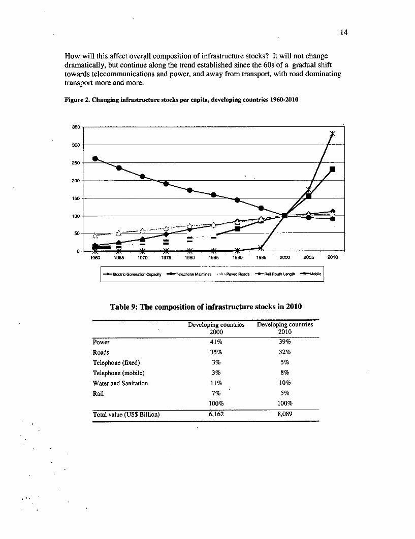
How will this affect overall composition of infrastructure stocks? It will not changedramatically, but continue along the trend established since the 60s of a gradual shifttowards telecommunications and power, and away from transport, with road dominatingtransport more and more.
Figure 2. Changing infrastructure stocks per capita, developing countries 1960-2010
Table 9: The composition of infrastructure stocks in 2010
Developing countries Developing countries2000 2010
Power 41% 39%
Roads 35% 32%
Telephone (fixed) 3% 5%
Telephone (mobile) 3% 8%
Water and Sanitation 11% 10%
Rail 7% 5%
100% 100%
Total value (US$ Billion) 6,162 8,089
15
Conclusion
We developed a model to predict future demand for infrastructure, which performs verywell in all sectors, even in water and sanitation where poor data usually makes estimationdifficult. It should be noted that ours are estimates of demand, rather than some absolutemeasure of "need." We also estimate needed resources for maintenance based on what isconsidered the minimum expenditure necessary to maintain the integrity of a system, andpredict total required resource flows to satisfy new demand and maintain service forexisting stocks.
Our overall estimates do not include resources that might be needed for rehabilitation ( tomake up for deferred past maintenance) or for upgrading. As such they are likely to belower bound estimates. Nevertheless they compare well with other studies estimates,notably with data on public expenditure on infrastructure from the 1980s.
The investments needed should amount to about $ 465 billion per annum or 5.5% ofdeveloping countries' GDP over 2005-2010. Most of it will go to the telecommunicationssector ($187 billion), followed by the power sector ($138 billion), and roads ($90 billion),including maintenance. Estimates for ports, airports and canals are not available, but sincethese types of infrastructure represent but a fraction of the total, it is unlikely thatincluding them would change our total estimates.
This study is an interesting, albeit limited, first foray into trying to systematically estimateinvestment needs. Like many study of its kind, it is surely broadly accurate in the orderof magnitude that it projects - notably concerning the inability of private investment tosatisfy demand in the near future. This work would however greatly benefit fromcomplementary studies, notably at individual country level.
16
Bibliography
Aschauer, David A. 1989. "Is public expenditure productive ?" Journal of MonetaryEconomics, Vol. 23, ppl77-200.
Canning, David. 1998. "A Database of World Infrastructure Stocks, 1950-95." PolicyResearch Working Papers no. 1929. The World Bank, Washington, DC.
Canning, David and Marianne Fay. 1993. The effect of Transportation Networks onEconomic Growth. Columbia University. Discussion Paper Series.
Easterly, William and Sergio Rebelo. 1993. "Fiscal Policy and Economic Growth: anEmpirical Investigation." National Bureau of Economic Research. Working Paper Series;No. 4499.
Fay, Marianne. 2000. "Financing the Future: Infrastructure Needs in Latin America,2000-05." World Bank Working Paper No. 2545. The World Bank, Washington DC.http://econ.worldbank.ora/resource.php
Ingram, Gregory K. and Marianne Fay. 1994. "Valuing Infrastructure Stocks and Gainsfrom Improved Performance.". Background Paper for the 1994 World DevelopmentReport. The World Bank, Washington, DC.
Moore, Edwin A. and George Smith, 1990. "Capital Expenditures for Electric Power inDeveloping Countries in the 1990s", World Bank Energy Series Paper No 21, WorldBank, Washington DC.
World Bank. 1994. "The World Development Report: Infrastructure for Development."Washington, DC.
17
Annex I
Data source and description
Telephone, number of main lines; electricity generating capacity in millions of watts;rail track length, in kilometers; and, paved roads length, in kilometers are from Canning(1998) for 1960 to 1995, available at:http://www.worldbank.ora/html/dec/Publications/WorkpapersMNPS1 900series/wDsl1929/canninc 1.xis.
Telephone, paved roads, mobile phones (in subscribers per 1000 inhabitants) are fromthe World Development Indicators (WDI) database of The World Bank(http:/Hwww.worldbank.org/data/.)
Rails for 2000 are from International Railways Statistics, available athttp://www.uic.asso.fr/d stats/stats en.html.
Electricity generating capacity for 2000 are from US Energy InformationAdministration, available at httD://www.eia.doe.gov/neic/historic/hinternational.htm.
Safe water is defined as percentage of population with reasonable access to an adequateamount of safe water, including treated surface water and untreated but uncontaminatedwater such as from springs, sanitary wells, and protected boreholes. In urban areas thismay be a public fountain or standpipe located no more than 200 m from the dwelling. Inrural areas, the definition implies that members of the household do not have to spend adisproportionate part of the day fetching water. Sanitation is defined as percentage ofpopulation with at least adequate excreta disposal facilities that can effectively preventhuman, animal and insect contact with excreta. Suitable facilities range from simple butprotected pit latrines to flush toilets with sewerage connection. Data are from the WDIdatabase of The World Bank (http://www.worldbank.6rg/data/.)
GDP and GDP per capita are from the World Development Indicators and are expressedin constant 1995 dollars. Data are from the WDI database of The World Bank(http://www.worldbank.orn/data/.)
Agriculture share and manufacture share of value added are expressed in percentageare from the WDI database of The World Bank (http://www.worldbank.org/datal.)
Total population and urban population, in percentage are from the United NationsPopulation Projections (http://www.un.org/popin/wdtrends.htm)
Annex IIExpected annual investment needs 2005-2010, $ millions
New |Paved
Electricity Telephone Road Rail RoadGeneration Mainlines Length Length Mobile Water Sanitation Total
East Asia & Pacific 25,005 17,041 12,133 164 41,15 1,799 2,608 99,90South Asia 11,124 3,233 6,575 12 3,39 1,91 1,707 28,069Europe & Central Asia 12,643 5,157 9,800 743 9,74 23 750 39,069Middle East & North Africa 7,30 1,278 3,308 51 1,85 39 691 14,88Sub-Saharan Africa 3,273 539 4,09 14 3,27 689 1,256 13,26Latin America & Caribbean 15,034 3,276 2,791 15,04 64 1,14 37,944High income 37,051 8,706 77,05 1 11,595 56 98 135,95Low Income 17,99 4,835 13,59 491 6,393 2,974 3,706 49,98Middle Income 56,39 25,690 25,104 733 68,068 2,70 4,454 183,151Developing Regions 74,38 30,525 38,702 1,22 74,461 5,681 8,160 233,13WORLD 111,436 39,231 115,758 1,225 86,056 6,246 9,143 369,095
MaintenanceEast Asia & Pacific 18,373 16,838 8,475 1,426 26,070 3,602 4,202 78,986South Asia 6,98 3,404 15,753 1,372 1,815 3,28 2,41 35,03Europe & Central Asia 20,333 6,67 16,454 4,035 7,298 1,43 2,616 58,849Middle East & North Africa 4,625 1,569 3,61 450 1,344 62 1,03 13,264Sub-Saharan Africa 2,941 653 3,429 873 2,181 949 1,619 12,644Latin America & Caribbean 10,593 4,175 4,128 733 10,015 1,24 1,989 32,87
Annex IIExpected annual investment needs 2005-2010, as % of GDP
New _Electricity Telephone Paved Road Rail RoadGeneration Mainlines Length Length Mobile Water Sanitation Total
East Asia & Pacific 0.929' 0.639' 0.459' 0.019' 1.51% 0.079' 0.109' 3.67%South Asia 1.219' 0.359' 0.729' 0.019' 0.37% 0.219' 0.19% 3.06%Europe & Central Asia 0.899' 0.369' 0.699' 0.059' 0.69% 0.029' 0.059' 2.76%Middle East & North Africa 1.169' 0.209' 0.539' 0.019' 0.29% 0.069' 0.119' 2.37%Sub-Saharan Africa 0.709' 0.129' 0.88% 0.03% 0.70% 0.159' 0.27% 2.84%Latin America & Caribbean 0.649' 0.14% 0.12% 0.009' 0.64% 0.039' 0.05% 1.62%High income 0.11% 0.03% 0.24% 0.009' 0.049' 0.009' 0.00% 0.42%Low Income 1.15% 0.31% 0.879' 0.039' 0.419' 0.199' 0.249' 3.18%Middle Income 0.81% 0.37% 0.36% 0.019' 0.989' 0.049' 0.069' 2.64%Developing Regions 0.889' 0.369' 0.469' 0.019' 0.889' 0.079' 0.109' 2.74%WORLD 0.279' 0.109' 0.28% 0.009' 0.21% 0.029' 0.029' 0.90%
MaintenanceEast Asia & Pacific 0.67% 0.62% 0.3 1% 0.05% 0.96% 0.139' 0.159' 2.90%South Asia 0.769' 0.379' 1.729' 0.15% 0.20% 0.369 0.269' 3.82%Europe & Central Asia 1.44% 0.47% 1.169' 0.29% 0.52% 0.109' 0.189' 4.16%
iddle East & North Africa 0.74% 0.259' 0.58% 0.07% 0.21% 0.109 0.169' 2.11%Sub-Saharan Africa 0.639' 0.149' 0.739' 0.19% 0.47% 0.209 0.359' 2.71%Latin America & Caribbean 0.45% 0.189' 0.189' 0.03% 0.43% 0.059 0.089' 1.40%High income 0.249' 0.079' 0.289' 0.02% 0.11% 0.01% 0.029' 0.76%Low Income 0.859' 0.349' 1.469' 0.199 0.24% 0.329 0.359' 3.73%Middle Income 0.739X 0.40% 0.429' 0.09% 0.65% 0.099 0.129' 2.50%Developing Regions 0.759' 0.39% 0.619' 0.109 0.57% 0.13 0.16' 2.73%WORLD 0.35% 0.14% 0.35' 0.049' 0.209' 0.04% 0.05' 1.17%
I
Policy Research Working Paper Series
ContactTitle Author Date for paper
WPS3087 Gender, Generations, and Nonfarm M. Shahe Emran June 2003 P. KokilaParticipation Misuzu Otsuka 33716
Forhad Shilpi
WPS3088 U.S. Contingent Protection against Julio J. Nogu6s June 2003 P. FlewittHoney Imports: Development Aspects 32724and the Doha Round
WPS3089 The "Glass of Milk" Subsidy Program David Stifel June 2003 H. Sladovichand Malnutrition in Peru Harold Alderman 37698
WPS3090 The Cotonou Agreement and its Manuel de la Rocha June 2003 F. SyImplications for the Regional Trade 89750Agenda in Eastern and Southern Africa
WPS3091 Labor Market Policies and Pierre-Richard Agenor July 2003 M. GosiengfiaoUnemployment in Morocco: Karim El Aynaoui 33363A Quantitative Analysis
WPS3092 The Integrated Macroeconomic Model Pierre-Richard Agenor July 2003 M. Gosiengfiaofor Poverty Analysis: A Quantitative Alejandro lzquierdo 33363Macroeconomic Framework for the Hippolyte FofackAnalysis of Poverty Reduction Strategies
WPS3093 Migration and Human Capital in Norbert M. Fiess July 2003 R. IzquierdoBrazil during the 1990s Dorte Verner 84161
WPS3094 Oil, Agriculture, and the Public Norbert M. Fiess July 2003 R. lzquierdoSector: Linking Intersector Dynamics Dorte Verner 84161in Ecuador
WPS3095 The Emerging Project Bond Market: Mansoor Dailami July 2003 S. CrowCovenant Provisions and Credit Robert Hauswald 30763Spreads
WPS3096 International Survey of Integrated Jose de Luna Martinez July 2003 S. CocaFinancial Sector Supervision Thomas A. Rose 37474
WPS3097 Measuring Up: New Directions for Piet Buys July 2003 Y. D'SouzaEnvironmental Programs at the Susmita Dasgupta 31449World Bank Craig Meisner
Kiran PandeyDavid WheelerKatharine BoltKirk HamiltonLimin Wang
WPS3098 Governance and Economic Growth Mark Gradstein July 2003 H. Sladovich37698
WPS3099 Creating Partnerships for Capacity F. Desmond McCarthy July 2003 D. PhilageBuilding in Developing Countries: William Bader 36971The Experience of the World Bank Boris Pleskovic
WPS3100 Governance of Communicable Monica Das Gupta July 2003 H. SladovichDisease Control Services: A Case Peyvand Khaleghian 37698Study and Lessons from India Rakesh Sarwal
Policy Research Working Paper Series
ContactTitle Author Date for paper
WPS3101 Portfolio Preferences of Foreign Reena Aggarwal July 2003 A. YaptencoInstitutional Investors Leora Klapper 31823