Leonardo Becchetti – Annalisa Castelli – Iftekhar Hasan

Investment-cash flow sensitivities, credit rationing and financing constraints

Bank of Finland ResearchDiscussion Papers15 • 2008

Suomen Pankki Bank of Finland

PO Box 160 FI-00101 HELSINKI

Finland +358 10 8311

http://www.bof.fi

Bank of Finland Research Discussion Papers 15 • 2008

Leonardo Becchetti* – Annalisa Castelli* – Iftekhar Hasan**

Investment-cash flow sensitivities, credit rationing and financing constraints

The views expressed in this paper are those of the authors and do not necessarily reflect the views of the Bank of Finland. * Department of Economics and Institutions, Faculty of

Economics, University of Rome “Tor Vergata”. ** Lally School of Management and Technology, Rensselaer

Polytechnic Institute, Troy, NY 12180-3590 and Bank of Finland. E-mail: hasan@rpi.edu.

We thank Jerry Dwyer, Zeno Rotondi, Enrico Santarelli, Chris Tucci, A. Zazzaro and participants of the seminars at the Lally School of Management of Rensselaer Polytechnic Institute, Capitalia, Rome, and at the University of Naples (SUN) seminar for useful comments and suggestions. The usual disclaimer applies.

http://www.bof.fi

ISBN 978-952-462-446-6 ISSN 0785-3572

(print)

ISBN 978-952-462-447-3 ISSN 1456-6184

(online)

Helsinki 2008

3

Investment-cash flow sensitivities, credit rationing and financing constraints

Bank of Finland Research Discussion Papers 15/2008

Leonardo Becchetti – Annalisa Castelli – Iftekhar Hasan Monetary Policy and Research Department Abstract

The controversy over whether investment-cash flow sensitivity is a good indicator of financing constraints is still unresolved. We tackle it from several different angles and cross-validate our analysis with both balance sheet and qualitative data on self-declared credit rationing and financing constraints. Our qualitative information shows that (self-declared) credit rationing is (weakly) related to both traditional a priori factors – such as firm size, age and location – and lenders’ rational decisions based on their credit risk models. We use our qualitative information on firms that were denied credit to provide evidence relevant to the investment-cash flow sensitivity debate. Our results show that self-declared credit rationing significantly discriminates between firms that do and do not have such sensitivity, whereas a priori criteria do not. The same result does not apply when we consider the wider group of financially constrained firms (which do not seem to have a higher investment-cash flow sensitivity), which supports the more recent empirical evidence in this direction. Keywords: financing constraints, credit rationing, investment/cash flow sensitivity JEL classification numbers: D92, G21

4

Aiheuttavatko luotonsäännöstely ja rahoitusrajoitteet riippuvuuden yritysten investointien ja kassavirran välille?

Suomen Pankin keskustelualoitteita 15/2008

Leonardo Becchetti – Annalisa Castelli – Iftekhar Hasan Rahapolitiikka- ja tutkimusosasto Tiivistelmä

Yritysten investointien ja kassavirran välisen korrelaation tulkinnasta käydään taloustieteissä yhä vilkasta keskustelua. Viime kädessä kysymys on siitä, aiheu-tuuko investointien havaittu riippuvuus kassavirrasta yritykseen kohdistuvista rahoitusrajoitteista vai reagoivatko investoinnit sittenkin yrityksen tulo-odotusten muutoksiin, joita kassavirran vaihtelut ilmentävät. Tässä tutkimuksessa investoin-tien kassavirtaherkkyyttä rahoitusrajoitteiden indikaattorina tarkastellaan empiiri-sesti eri näkökulmista. Tarkastelujen apuna käytetään sekä yritysten tasetietoja että kvalitatiivisia kyselyaineistoja yrityksiin kohdistuvista luotonsääntelystä ja rahoitusrajoitteista. Yritysten kokema luotonsäännöstely korreloi käytetyn kvalita-tiivisen aineiston perusteella sekä perinteisten indikaattoreiden – kuten yrityksen koko, ikä ja maantieteellinen sijainti – että lainanantajien luottoriskimalleista las-kettujen päätösten kanssa. Korrelaatiot eivät tosin ole kovin vahvoja. Tarkastelu-jen yksi keskeinen ajatus on löytää näyttöä yhteydestä yritykseen kohdistuvan luo-tonsäännöstelyn sekä sen investointien ja kassavirran korrelaation voimakkuuden välillä. Tulosten mukaan yrityksen raportoimaa tietoa luotonsäännöstelystä voi-daan selvästi käyttää hyödyksi eroteltaessa toisistaan yritykset, joissa investoin-tien riippuvuus kassavirrasta on selvä, niistä yrityksistä, joissa tätä riippuvuutta ei ole havaittavissa. Perinteiset indikaattorit eivät ole tällaisen erottelun kannalta hyödyllisiä. Yrityksiin kohdistuvalla luotonsäännöstelyllä ei kuitenkaan ole vas-taavaa erotteluvoimaa laajemmin rahoitusrajoitteista kärsivien yritysten keskuu-dessa. Näiden yritysten investointien ja kassavirran välinen riippuvuus ei nähtä-västi ole vertailuryhmän yrityksiin verrattuna voimakkaampaa. Nämä tulokset ovat sopusoinnussa tuoreissa tutkimuksissa raportoidun empiirisen näytön kanssa. Avainsanat: rahoitusrajoitteet, luotonsäännöstely, investointien ja kassavirran kor-relointi JEL-luokittelu: D92, G21

5

Contents

Abstract .................................................................................................................... 3 Tiivistelmä (abstract in Finnish) .............................................................................. 4 1 Introduction ...................................................................................................... 7 2 Financing constraints, credit rationing and the KZ/FHP controversy ..... 11 3 The database ................................................................................................... 12 3.1 Some descriptive findings on the Capitalia sample ................................. 14 3.2 Some descriptive findings on credit rationing and financing constraints ................................................................................................ 14 4 Logit econometric findings: efficient screening vs discrimination ............ 16 5 Our approach to solve observational equivalence in econometric tests of financing constraints ......................................................................... 21 6 Results from Euler equation estimations ..................................................... 25 7 Conclusions ..................................................................................................... 27 References .............................................................................................................. 28 Tables 1–11 ............................................................................................................ 34 Appendix 1 ............................................................................................................. 40 Appendix 2 ............................................................................................................. 49

6

7

1 Introduction

A main point in the literature on the empirical tests on the existence of financing constraints remains unsettled. The controversy is represented by the criticism of Kaplan and Zingales (hereafter also KZ) (1997) about the well known Fazzari, Hubbard and Petersen (hereafter also FHP) (1988) results on the higher investment-cash flow sensitivity of financially constrained firms.1 KZ (1997) theoretically demonstrate that firm investment choices under profit maximising behaviour do not imply a monotonic relationship between financing constraints and the sensitivity of investment to cash flow. Therefore, they conclude, it is not correct to test for the existence of financing constraints by comparing investment cash-flow sensitivities of two subgroups based on given a priori cut-off criteria (ie small firms are financially constrained and large firms are not). This is because the cut-off does not necessarily separate a subgroup of more financially constrained firms in which the sensitivity is significantly higher, from one of less financially constrained firms in which the same sensitivity is significantly lower. To test empirically their point, the two authors consider the 49 low-dividend payout firms that FHP selected a priori as more financially constrained in a given historical period. By using qualitative and quantitative information they divide the available firm-year observations into five groups according to the degree of financing constraints revealed by qualitative information.2 They find that investment-cash flow sensitivity is not higher (it is in fact lower) for the subgroup of more financially constrained firm-year observations.3 Empirical findings similar to those of KZ are found by Cleary (1999) who uses multiple discriminant analysis to identify firm financing constraints and finds that less constrained firms are those whose investment is more sensitive to cash flow. An original theoretical interpretation of these findings comes from Almeida et al (2004) who analyse the demand of precautionary savings of constrained and unconstrained firms and find that financially constrained firms have a higher sensitivity of cash (reserves) to cash flow which justifies the observed reduced sensitivity of their investment to cash flow. Additional theoretical rationales supporting the criticism to the FHP interpretation of the investment-cash flow sensitivity come from Alti (2003). The author shows that FHP findings may simply result from a standard neoclassical model in which younger firms face uncertainty about their growth prospects and

1 Findings which do not contradict FHP (1988) results are those of Bond and Meghir (1994), Withed (1992) and Hoshi et al (1991). 2 The qualitative information is taken from the 10-K annual report containing information on financial conditions. 3 The authors test financing constraints directly with the investment-cash flow equation and are therefore subject to all the critiques related to problems in measuring the marginal Tobin’s q and the replacement cost of capital (Chirinko, 1993).

8

this uncertainty is resolved by cash flow realizations which, in part, represent the option value of their long-term growth potential. Calibration of the Alti (2003) model shows that investment is sensitive to cash flow for all firms after correcting for the Tobin’s q. In this model, investment-cash flow sensitivity is higher for younger and smaller firms with high growth rates since these firms learn about their project quality through cash flow realizations. In a similar way, Gomes (2001) and Abel and Eberly (2002 and 2004) develop frameworks in which positive investment-cash flow correlations arise in absence of financial market imperfections. FHP (2000) reply to KZ (1997) theoretical argument by identifying conditions under which the investment-cash flow sensitivity is larger for financially constrained firms. They argue that, as far as the constrained/unconstrained ratio of the second derivative of the supply curve for external finance is higher than the ratio of their marginal productivity of capital, the constrained group exhibits a higher investment-cash flow sensitivity (for analytical details on this point see section 2). Even though in this way they admit that the relationship between investment-cash flow sensitivity and financing constraints is non monotonic, FHP (2000) argue that the above mentioned condition on the slope of the supply of external finance is likely to be met for the a priori classification criteria (size, age, dividend payout, access to public debt) usually considered in the literature. This paper aims to provide an additional contribution to this literature. It shows how the combination of survey and balance sheet information on credit rationing may provide additional evidence and disentangle many of the joint hypothesis/observational equivalence problems which prevent to shed light on the alternative interpretations of the investment/cash flow sensitivity.4 More specifically, we argue that: i) the newly available qualitative information on self declared credit rationing

overcomes the KZ objection on the inaccuracy of the sorting criteria used for testing the correspondence between the investment/cash flow sensitivity and the presence of credit rationing. In section 2 we in fact show that, even though – according to KZ – such sensitivity is not monotonically increasing in the

4 Empirical papers closely related to our are those of Cole (1998) and Sapienza (2002). Cole (1998) uses survey data to examine the likelihood of credit denial for small US firms, finding that firms without pre-existing relationships, younger firms and smaller firms are more likely to be denied credit. Sapienza (2002) documents that Italian firms with higher leverage and lower profitability are more likely to lose their credit lines. The difference of our approach with Cole (1998) is in the matching of qualitative and balance sheet data and the use of qualitative information on credit denial to shed light on the investment/cash flow sensitivity debate. The difference with respect to Sapienza (2000) is that our analysis is not limited to target banks’ and borrower banks’ prior to bank acquisition and the focus is the loss of credit lines while ours is on the more general issue of credit denial (without reference to the previous existence of credit lines).

9

degree of financing constraints, it is definitely higher for credit rationed than for non credit rationed firms.5

ii) the combination of survey data and balance sheet information allows us to

disentangle the traditionally tested hypothesis (subgroups of firms defined according to a priori criteria exhibit excess investment/cash flow sensitivity and therefore are financially constrained) into three separate hypotheses: a) H0: a priori criteria used for subgroup classification significantly affect the probability of (self declared) financing constraints and/or credit rationing; b) H1: (self declared) credit rationed and/or financially constrained firms have higher investment/cash flow sensitivity; c) H2: a priori criteria used to discriminate among different degrees of financing constraints identify firms with higher investment/cash flow sensitivity (links among these hypotheses are illustrated in Figure 1).

Another contribution of this paper is in the construction of credit risk indicators based on the most relevant available results of the credit risk empirical literature.6 This allows us to test whether credit denial is the rational outcome of the application of lender’s credit risk measures or, alternatively, discrimination based on a priori criteria (size, age, etc). Finally, while most empirical papers on financing constraints work on samples of large companies listed at the US stock exchange, our paper focuses on a representative sample of mainly small and medium sized firms which are not public (the median size in our sample is 22 employees). We believe this is important since the impact of financing constraints or credit rationing on corporate behaviour may differ whether we consider large companies, which have alternative sources of external finance such as bond or equity issues, or small and medium sized companies, whose main source of external finance is bank debt. The paper is divided into seven sections (including introduction and conclusions).

5 For financing constraints we intend a wedge between the cost of external and internal finance. For credit rationing the impossibility of obtaining (additional) finance from external sources. 6 Our use of credit risk indicators is different from that of Cleary (1999). We use these variables as regressors in the estimate of the determinants of self declared credit rationing and not as sorting criteria used to test the investment/cash flow sensitivity of firms with financing constraints.

10

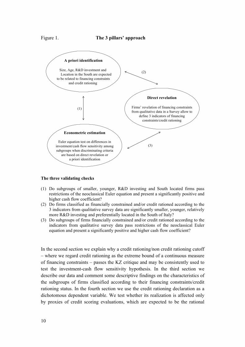
Figure 1. The 3 pillars’ approach

The three validating checks (1) Do subgroups of smaller, younger, R&D investing and South located firms pass

restrictions of the neoclassical Euler equation and present a significantly positive and higher cash flow coefficient?

(2) Do firms classified as financially constrained and/or credit rationed according to the 3 indicators from qualitative survey data are significantly smaller, younger, relatively more R&D investing and preferentially located in the South of Italy?

(3) Do subgroups of firms financially constrained and/or credit rationed according to the indicators from qualitative survey data pass restrictions of the neoclassical Euler equation and present a significantly positive and higher cash flow coefficient?

In the second section we explain why a credit rationing/non credit rationing cutoff – where we regard credit rationing as the extreme bound of a continuous measure of financing constraints – passes the KZ critique and may be consistently used to test the investment-cash flow sensitivity hypothesis. In the third section we describe our data and comment some descriptive findings on the characteristics of the subgroups of firms classified according to their financing constraints/credit rationing status. In the fourth section we use the credit rationing declaration as a dichotomous dependent variable. We test whether its realization is affected only by proxies of credit scoring evaluations, which are expected to be the rational

A priori identification

Size, Age, R&D investment and Location in the South are expected

to be related to financing constraintsand credit rationing

Direct revelation

Firms’ revelation of financing constraintsfrom qualitative data in a Survey allow to

define 3 indicators of financingconstraints/credit rationing

Econometric estimation

Euler equation test on differences ininvestment/cash flow sensitivity amongsubgroups when discriminating criteria

are based on direct revelation ora priori identification

(1)

(3)

(2)

11

outcome of the bank screening process, or also by ‘discrimination variables’ such as firm size, age, R&D investing status and geographical location. In the fifth and sixth sections we check the consistence among qualitative declarations, a priori criteria and the FHP test on investment-cash flow sensitivities. We estimate Euler equations for subgroups of firms in our sample, according to different sorting mechanisms based either on the traditional a priori criteria or on the qualitative declaration of credit constraints contained in our survey data. In the seventh section we comment our empirical findings. 2 Financing constraints, credit rationing and the

KZ/FHP controversy

To explain how we devise our test we start from the benchmark used by KZ (1997) and FHP (2000) in their controversy: a one period model in which a representative firm chooses I to maximise the following

)k,E(C)I(MaxF − (2.1) where F(I) is the revenue function, I = W+E is investment which can be financed with internal (W) or external finance (E), while C(.) is a cost function convex in E (the amount of external funds raised) and depending on (k), a measure of the firm’s wedge between internal and external finance. By implicitly differentiating the first order condition we obtain an expression for the investment-cash flow sensitivity on which both KZ (1997) and FHP (2000) agree

1111

11

FCC

dWdI

−= (2.2)

where C11 is the second derivative of the cost function with respect to external finance and F11 is the slope of the marginal productivity of investment. We start from the definition of financing constraints in which financially constrained firms are intended as those having a positive wedge between the cost of external and internal finance. As far as the intensity of financing constraints is higher, we end up to a point in which firms are refused additional credit at the existing interest rate. We may then consider this type of credit rationing as the

12

extreme which delimits the interval of a continuous measure of the intensity of financing constraints.7 Consider that, if we use as cut-off the rationing/non rationing status, we definitely meet the FHP (2000) and Zingales (1997) condition (equation 2) for the correspondence between higher financing constraints and higher investment cash-flow sensitivity. Credit rationing in fact implies that C11 tends to infinite and,

therefore, 1dWdIlim

11C=

∞→, while, under the standard assumptions of F1 > 0 and

F11 < 0, dI/dw < 1 for the subgroup of non credit rationed facing less than infinite marginal cost of external finance. Hence, the latter have an investment/cash flow sensitivity which is significantly lower than that of credit rationed firms.8 A similar reasoning considers that, under the assumption that the denied credit would have been used for investment, credit rationed firms are able to finance

with bank debt only a share α of their planned investment with 1111

11

FCC

dWdI

−= ,

while, for the remaining share (1–α), their sensitivity of investment to cash flow is, by definition, equal to one. On the contrary, non financially constrained firms succed in financing all their investment and, therefore, their sensitivity coincides

with 1111

11

FCC

dWdI

−= . As far as α gets smaller in the credit rationed subgroup,

marginal and average investment/cash flow sensitivity coincide and are necessarily higher than the corresponding average and marginal values for the non credit rationed subgroup. 3 The database

The opportunity of discriminating among the above mentioned different conclusions on the significance of the investment-cash flow sensitivity is provided by a unique source of information, the Capitalia Survey, which is the most important, periodically repeated, quantitative-qualitative survey on Italian firms.9

7 Consider that KZ (1997) have similar information for the fifth subgroup of firm-year observations which they define as undoubtedly financially constrained. In this group they include companies ‘in violation of debt covenants, cut out of the usual source of credit, renegotiating debt payment or forced to reduce investments for liquidity problem’. It is likely that some of these firms would fall into our credit rationed subgroup. Since firm-year observations for these firms are too few, KZ do not test the investment-cash flow sensitivity on this specific subgroup. 8 Credit denial implies that the supplier of credit is not available to provide additional finance at any (no matter how higher) interest rate and is therefore equivalent as saying that the price for external finance for the borrower approaches infinity. 9 The Survey has been previously known as Mediocredito Centrale Survey and the related questionnaire is entirely reported in Appendix 2.

13

The survey has been repeated every three years, starting from 1989, on a sample of around 4,500 firms with more than 9 employees. In order to maintain representativeness and take into account the high exit/entry rate of firms in the Italian market, the original sample has been reshaped for each wave. The different waves have been stratified by size classes based on the number of employees, geographical areas and macrosectors according to the Pavitt (1984) classification.10 The value added per employee has been used as a stratifying factor. For the purpose of this study we start from the last wave of the survey (1998–2000) and match information on firm financial status and balance sheet data from the previous waves. Balance sheet and income statement data come from the CERVED and AIDA databases. Qualitative data are obtained from questionnaires answered by a representative of each firm and then checked for inconsistencies.11 From the overall sample, we select firms for which complete balance sheet and income statement are available. We select firms with positive values of total assets, net worth and net sales.12 The result is a balanced panel of 3,840 firms for the period 1992–2000 (Capitalia survey merged with balance sheets from CERVED and AIDA databases).

10 Size classes: 11–20; 21–50; 51–250; 251–500; more than 500. Macroareas: North East (Trentino Alto Adige, Veneto, Friuli Venezia Giulia and Emilia Romagna), North West (Piemonte, Valle d’Aosta, Lombardia and Liguria), Central Regions (Toscana, Umbria, Marche and Lazio), South and Isles (Abruzzo, Molise, Campania, Puglia, Basilicata, Calabria, Sicilia and Sardegna). Pavitt sectors: Scale Economies, Specialised, Traditional and High tech. 11 All balance sheet data in the Capitalia Survey database are accurately checked. These data come from official sources: the CERVED database (first sample period) and AIDA – Bureau Van Dijk database (last two sample periods) which collects from CERVED all balance sheets for the same firms. CERVED obtains the information from the Italian Chambers of Commerce and is currently the most authoritative and reliable source of information on Italian companies. Qualitative data from questionnaire are filled by a representative appointed by the firm collecting information from the relevant firm division. The questionnaire has a system of controls based on ‘long inconsistencies’, namely inconsistencies between answers to questions placed at a certain distance in the questionnaire. In case of inconsistent information the firm is subject to a second phone interview. Firms which do not provide reliable information after being recontacted are excluded from the sample. A supplementary list of 8000 firms is built for each of the three year surveys in order to avoid that exclusions generated by missing answers or inaccuracies in the questionnaire, may alter the sample design. Substitutions follow the criteria of consistency between the sample size and the population of the Universe. 12 In order to eliminate the influence of extreme values we follow the procedure adopted by Cleary (1999) and winsorize the data according to the following rules: i) return on equity (ROE) greater than 100 per cent or lower than -20 per cent; ii) return on assets (ROA) greater than 30 per cent or lower than -20 per cent; iii) ratio of total sales to total assets greater than 300 per cent or lower than 20 per cent; iv) ratio of investment to net fixed assets greater than 50 per cent; v) ratio of total sales to net fixed assets grater than 400 per cent; vi) ratio of cash flow to net fixed assets grater than 50 per cent; vii) ratio of total debt to net fixed assets grater than 200 per cent. Results presented in the next sections are nonetheless robust to the inclusion of outliers. Evidence on this point is available from the authors upon request.

14

3.1 Some descriptive findings on the Capitalia sample

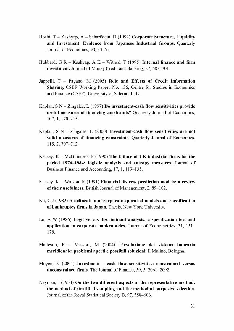
We inspect the properties of our balanced sample by looking at characteristics of firms by size classes (Table 1).13 Large firms are much older than small firms (approximately 39 against 23 years). Firms are also generally smaller in the Center and South of Italy. As expected, large firms are affiliated to groups (around 84 per cent against 12 per cent) and export (around 94 per cent against 64 per cent) in a much higher proportion than small firms. Significant differences in size classes also arise in R&D expenditures (76 per cent against 31 per cent). The reader can verify that medium firms are somewhere in the middle between these two extremes for each of the above mentioned variables. When we look at bank-firm relationships we find that small firms have in higher proportion the first lender located in their same province (65 per cent against 47 per cent of large firms). Large firms have, on average, commercial relationships with around 10 different banks, while small firms only with 5. As expected, the share of debt held by the first lender is larger in small firms (41 against 19 per cent) and its relationship with the borrower is younger (17 against 19 years). Finally, a higher share of large firms obtains government subsidies (60 per cent against 38 per cent). 3.2 Some descriptive findings on credit rationing and

financing constraints

To identify the subsample of credit rationed firms we consider the following questions in the survey: 1) in the year 2000 had the company desired more credit at the market interest rate? In case of affirmative answer the following two questions are asked: 2) had the company been willing to pay a higher interest rate in order to obtain more credit? 3) Did the company demanded in the year 2000 more credit without obtaining it? We classify as highlyrationed firms those answering positively to all of the three questions, deniedcred firms those answering positively to questions 1) and 3) and desirecred firms all firms answering affirmatively to question 1) (even when they do not answer positively to questions 2 and 3). These three classifications identify some potential differences in the intensity of financing constraints. Consider, in fact, that an affirmative response to question 2) indicates the existence of a positive difference between demand and supply of 13 We adopt here the standard EU classification which considers as small firms those below 50 employees, as medium firms those between 50 and 250 employees and as large firms those above 250 employees.

15

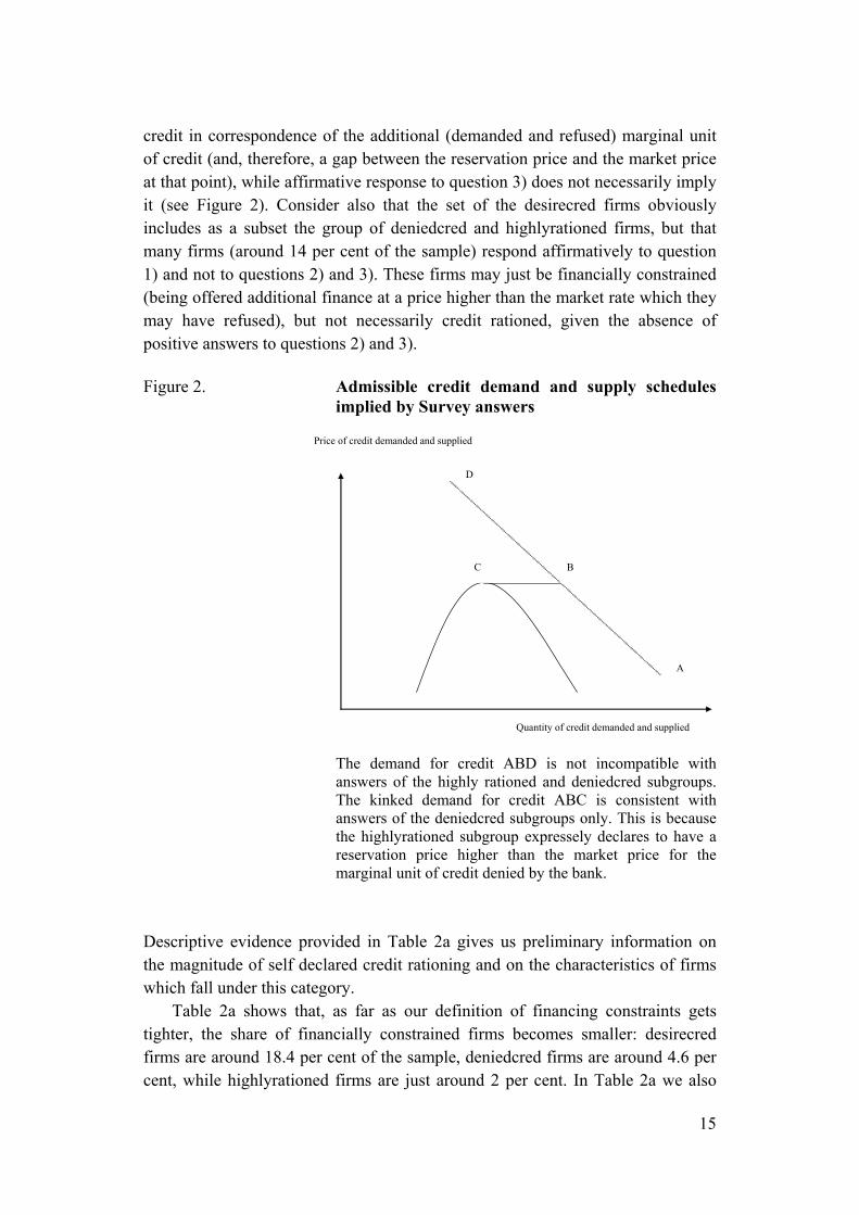
credit in correspondence of the additional (demanded and refused) marginal unit of credit (and, therefore, a gap between the reservation price and the market price at that point), while affirmative response to question 3) does not necessarily imply it (see Figure 2). Consider also that the set of the desirecred firms obviously includes as a subset the group of deniedcred and highlyrationed firms, but that many firms (around 14 per cent of the sample) respond affirmatively to question 1) and not to questions 2) and 3). These firms may just be financially constrained (being offered additional finance at a price higher than the market rate which they may have refused), but not necessarily credit rationed, given the absence of positive answers to questions 2) and 3). Figure 2. Admissible credit demand and supply schedules

implied by Survey answers

The demand for credit ABD is not incompatible with

answers of the highly rationed and deniedcred subgroups. The kinked demand for credit ABC is consistent with answers of the deniedcred subgroups only. This is because the highlyrationed subgroup expressely declares to have a reservation price higher than the market price for the marginal unit of credit denied by the bank.

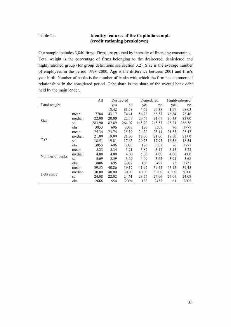
Descriptive evidence provided in Table 2a gives us preliminary information on the magnitude of self declared credit rationing and on the characteristics of firms which fall under this category. Table 2a shows that, as far as our definition of financing constraints gets tighter, the share of financially constrained firms becomes smaller: desirecred firms are around 18.4 per cent of the sample, deniedcred firms are around 4.6 per cent, while highlyrationed firms are just around 2 per cent. In Table 2a we also

Quantity of credit demanded and supplied

A

B

D

C

Price of credit demanded and supplied

16

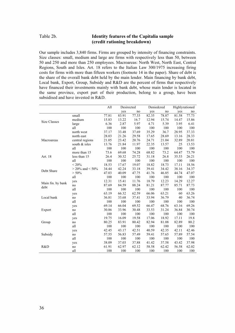
find that firms belonging to the three subgroups of financially constrained firms are smaller than the complementary sample (desirecred firms have mean and median size of respectively 43 and 20 employees against 74 and 22 of the control sample). Financially constrained firms are also younger in both mean and median with a difference with respect to the complementary sample ranging between 1 and 3 years. With regard to the credit rationing geographical breakdown, Table 2b shows that, while only 14 per cent of sample firms are located in the South, this share jumps to 22 (25) per cent when we consider the deniedcred (highlyrationed) subgroup. In the same way, firms below 15 employees are 26 per cent in the overall sample and 31 (36) per cent in the deniedcred (highlyrationed) subgroup.14 Descriptive evidence provided in Table 3 also suggests that both the deniedcred and desirecred subgroups underperform with respect to their complementary samples in terms of both ROI and ROE which are up to 2 to 3 points lower in both mean and median. The difference in leverage among subgroups is also quite strong. For the deniedcred subgroup we observe a 10 point difference in median with respect to the control sample (0.18 against 0.8) which is reduced to a 5 point difference in the desirecred subgroup. The financial situation of the three subgroups is also worsened by the fact that highlyrationed firms have a median interest on net sales ratio of 4% against the 3% of the deniedcred and desirecred subgroups and the 2% of the overall sample.15 On the other hand, we observe that mean and median productivity per worker (net sales per worker) among the same subgroups are not so different, even though firms in the three subgroups appear slightly less productive than the complementary sample. 4 Logit econometric findings: efficient screening

vs discrimination

The literature of financing constraints has today its main focus on theoretical models and empirical tests aimed to solve the question of the relationship between the investment-cash flow sensitivity and the existence of financing constraints. 14 This threshold of 15 employees identifies a discontinuity in firing costs determined by an Italian law (Law 300/1975) which establishes that workers fired by firms with more than fifteen employees must be reintegrated in their workplace if a judge concludes that they have been fired without giusta causa (ie fair grounds). The same ‘fair grounds’ rule cannot be applied to workers fired in firms with less than 15 employees 15 More in detail, by observing the subgroup distribution of this variable at some relevant points we find that more than 25 per cent of the deniedcred (19 per cent of the desirecred) firms are above 50 per cent in the interest payment/net sales ratio against the 9 per cent (8 per cent) of the non deniedcred (non desirecred) firms. In the same way, more than 24 per cent (16 per cent) of deniedcred firms (desirecred firms) have an average leverage above .40 against about 10 per cent of firms in their respective complementary samples having leverage above that level.

17

We want to enlarge this focus by testing a related hypothesis which has relevant normative consequences. Are financing constraints under the extreme form of credit rationing the rational outcome of bank credit scoring processes based on balance sheet indicators? How much additional environmental variables (geographical location, size, age, R&D investment) matter in the credit rationing decisions? Were rationed firms relatively less productive ex ante than the rest of the sample? We test these hypotheses by combining the traditional expected determinants of financing constraints in the specific literature with those identified as enhancing borrower risk in the bankruptcy risk literature. This literature has grown extensively since Beaver (1966) and Altman (1968) proposed the use of linear discriminant analysis to predict firm bankruptcy. After these first contributions, discrete dependent variable econometric models, namely logit or probit models, have become the most popular tools for credit scoring.16 The main commercial application using logistic approach for default estimation is the Moody’s KMV Risk-Calc Suite of models developed for several countries.17 In recent years, alternative approaches using non parametric methods have been developed. These include classification trees, neural networks, fuzzy algorithms and k-nearest neighbours. Since our sample is mostly composed by non listed firms, we focus on corporate credit risk modelling for privately held firms in order to choose credit scoring measures adequate to our needs. Although firms with unlisted equity or debt represent a significant fraction of the corporate sector worldwide, research in this area has been hampered by the scarce availability of public data. This implied that, for privately held firms, accounting based credit scoring models have been mostly applied.18 Table A1.1 in Appendix 1 reports the results of a selection of some of the most important published credit risk papers with the identification of the estimated vector of variables and parameters which maximize the likelihood that a borrower is going to fail. We test whether some of these credit risk predictors have relevance if added to the vector of traditional determinants of financing constraints. In order to avoid correlation problems between balance sheet indicators and credit risk predictors we test the balance sheet and credit risk variables separately, in the following two logit model specifications written in compact form

16 See Barniv and McDonald (1999) for a detailed survey on the issue. 17 See Dwyer et al (2004). 18 Although credit scoring has well known disadvantages (see for example Allen, 2002), it remains the most effectively and widely used methodology for the evaluation of privately-held firms’ risk profiles.

18

i

6

1kikk

12

1jijj0i BalanceIdentity)Fc(Raz ε+γ+α+α= ∑∑

== (4.1)

i

7

1lill

12

1jijj0i eCreditscorIdentity)Fc(Raz ε+δ+α+α= ∑∑

== (4.2)

where the dependent variable Raz(Fc) is, alternatively, one if the firm belongs to the desirecred, deniedcred or highlyrationed subgroup and zero otherwise. Our twelve identity variables include ten dichotomous dummies (Small, Young, South and Isles, Export, Group, R&D, Local bank, Main fin. by bank debt, Subsidy and Art. 18) taking the value of one if the firm has the relevant characteristic and zero otherwise. Among them, Local bank is a dummy for firms whose main lender’s headquarter is located in the same province, Main fin. by bank debt is a dummy for firms whose main source of external finance is bank debt and the Art. 18 dummy takes the value of one for firms with less than 15 employees and zero otherwise. This variable tests the effect on credit rationing of the discontinuity in firing costs established by an Italian law (Law 300/1975) which states that workers fired by firms with more than 15 employees must be reintegrated in their workplace if they are judged to have been fired without giusta causa (ie fair grounds). The remaining Identity variables are Number of banks (number of different banks with which the firm has commercial relationships), Debt share (share of bank debt on total non short term debt). Our vector of balance sheet variables (Balance) includes the following regressors calculated on 1998 balance sheet values: ROS, ROI, ROE, Leverage, Interests on Net Sales and Net Sales per worker which measure, respectively, the value of operating profits over net sales, operating profits over total assets, net earnings over net worth, firm leverage debt, interest payments over net sales and net sales over the number of workers. Finally, we identify a vector of credit risk indicators (Creditscore) as follows. We select a limited number of published empirical papers (Table A1.1 in Appendix 1) in which credit risk measures have been successfully tested out of sample in given periods and countries. We calculate 1998 values for the credit risk predictor by applying the methodology of each of these papers. Unfortunately our data do not allow to construct all the credit risk indicators reviewed.19 The scoring variable is therefore introduced as an additional regressor in our estimate where we test, one by one, the inclusion of the credit scores from each of the reviewed papers. Results of specifications including insignificant indicators are omitted for reasons of space and are available upon request. The indicators which result significant and are finally selected are those suggested by Altman (1984), Altman, Baidya and Riberio-Dias (1979), Zmijeski (1984), Shumway (2001) and Saretto 19 Indicators tested are the ones marked with * in table A1.1 in Appendix 1.

19

(2004).20 The correlation matrix between balance sheet and credit risk indicators is provided in Table 4. All estimates in different specifications are run at a constant number of observations to avoid that our results be driven by sample selection effects caused by missing variables. Results are presented in Tables 5, 6, 7 and 8 where we test, respectively, the determinants of affiliation to the group of desirecred (but non deniedcred and non highlyrationed), of deniedcred and of highlyrationed. The question whether rationed firms were ex ante more indebted has undoubtedly a positive answer. Table 5 shows that rationed firms have significantly higher interest payment/net sales ratios. The inclusion of the significant credit risk indicators (Tables 6, 7 and 8) shows that financially constrained firms would result as significantly more riskier if bank screening were based on the reported risk measures. According to the Altman’s indicator (1984) a high Z-score is associated with a good financial position of the firm and this means that the negative sign we find in logit estimates is consistent with our interpretation of efficient screening. On the other side, the Zmijeski’s indicator (1984) is increasing in the probability of failure which is, again, consistent with the positive sign we get in logit estimates.21 The interesting finding though, is that, after correcting for performance, indebtedness and risk measures, identity variables such as location in the South, size, R&D investment status, age and the number of banks still remain (weakly or strongly) significant, even though only in some of the presented estimates. Our interpretation is that credit rationing is a mix of efficient screening and discrimination from the lender. On the one hand, the significance of the reported credit risk indicators leads us to consider the imposition of financing constraints as an efficient screening process and not as discrimination among firms with similar performance characteristics. On the other hand, the (weak or strong) significance of identity variables after correcting for performance, indebtedness and risk measures may be explained in two different ways. First, these variables are proxies for additional risk factors not captured by previously considered balance sheet indicators. Second, we have enough measures of risk, indebtedness and performance in the estimate to capture all risk dimensions and, therefore, the

20 Shumway (2001) and Saretto (2004) reproduce both Altman (1984) and Zmijeski (1984) indicators proposing different approaches for their estimations and applying them to different samples. For this reason we consider two indicators for Shumway (2001) (Shumway Altman and Shumway Zmijeski) and two for Saretto (2004) (Saretto Altman and Saretto Zmijeski). 21 The Z-model implies that all the accounting ratios included in the function have positive coefficients. And this is in fact true for the Altman (1984), Altman Baydia (1979) and Saretto (2004) Altman indicators. On the contrary Altman’s coefficients, as estimated by Shumway (2001), have negative signs and this explains the counterintuitive sign of the Shumway–Altman indicator in our logit estimates. The same is true for the negative sign of the Zmijeski Up (Unweighted Probit) indicator whose coefficients have positive sign.

20

significance of identity variables supports the hypothesis of discrimination of firms along these characteristics. The intepretation of the significance of some of the identity variables deserves further attention. With regard to the South variable, consider that the wave of mergers and acquisitions occurred in the Italian banking system in the 90’s has transferred, for large part, ownership of overindebed banks of the South in the hands of banks of the North.22 The empirical analysis on the effects of this change shows that the process of bank concentration and ownership transfer has increased bank performance (Focarelli et al, 2002) but some authors, on the other side, complain that it has also generated a loss of local information and reduced credit to local firms, as shown by the dramatic drop in the total volume of financed investment in the area (Mattesini and Messori, 2004). This should explain why location in the South is significant in the credit rationing estimate in the 1998–2000 sample and not in the 1989–1991 sample (Bagella et al, 2001). The alternative interpretation however is that the South variable proxies risk factors not captured by credit risk indicators. To this purpose Guiso, Sapienza and Zingales, (2004) and Jappelli, et al (2005) specifically show that regional differences in the efficiency of the Italian courts has a notable effect on the availability of credit to small businesses. Another important result (the inverse relationship between size and credit rationing) seems to be a constant in Italian empirical analyses on financing constraints (Bagella et al, 2001). The important additional point in our estimate is that, with the exception of the desirecred subgroup, we find that, being below the 15 worker threshold generates an additional significant effect on the probability of being credit rationed, net of the effect of being below the 50 worker threshold, measured by our size dummy (Table 5). As already mentioned above and in section 3.2, we test the impact of this additional threshold since regulation of the Italian job market establishes significantly lower firing costs for firms below 15 employees, thereby creating a downsizing incentive. Our analysis does not reject the hypothesis that the incentive to remain small produced by the law has negative consequences on the availability of external finance (Tables 5–8). Another apparently unexpected result is the significance of the local bank dummy on the desirecred (but not on the deniedcred and highlyrationed) variable. The two most likely interpretations are that: i) a relationship with a local (and presumably smaller) bank is a signal of firm weakness; ii) if credit markets are segmented the local bank has some monopoly power which translates into a wedge between external and internal finance. Finally, an apparently counterintuitive finding is the weak positive effect of the number of lenders, but only when the dependent variable is represented by

22 Some relevant examples of it are Banco di Napoli acquired by S. Paolo IMI, Banco di Sicilia acquired by Capitalia and Banco di Sardegna acquired by Cassa di Risparmio di Reggio Emilia.

21

affiliation to the deniedcred subgroup (Table 5). This is at odd with the hypothesis of Detragiache, Garella and Guiso (2000) who argue that multiple banking reduces the probability of credit rationing and von Thadden (1995) finding that a higher number of lenders reduces banking rent extraction. On the other side, though, it is compatible with results of Bolton and Scharfstein (1996) showing how multiple banking may make debt renegotiation more difficult and, mainly, with those of Petersen and Rajan (1994) showing that the passage from single to multiple borrowing increases the cost of credit and reduces its availability. Furthermore, the choice of multiple borrowing may be pursued by the firm to increase its ‘opacity’ with the result of a relatively lower production of information in equilibrium. Overall, our results suggest a profile of credit rationed firms as firms which tend to be relatively small and preferentially located in the South. Credit rationed firms are also more indebted on average and financially constrained firms have higher scores in terms of credit risk indicators (Tables 6–8).23 5 Our approach to solve observational equivalence

in econometric tests of financing constraints

Four are the main methods employed in the financing constraints empirical literature to test the investment/cash flow relationship: i) the direct estimate of the investment demand function obtained from first order conditions of standard profit maximization in which the shadow value of capital (marginal Tobin’s q) is proxied by the average Tobin’s q (Fazzari, Hubbard and Petersen, 1988; Gertler and Hubbard, 1988; Kaplan and Zingales, 1997 and 2000, for the US; Hayashi-Inoue, 1988; Hoshi, Kashyap and Sharfstein, 1991, for Japan; Devereux and Schiantarelli, 1989; Schiantarelli and Georgoutsos, 1990, for the UK); ii) the Euler equation approach which combines two first order conditions to avoid the inclusion of the marginal Tobin’s q among regressors when testing for financing constraints (Bond and Meghir, 1994; Withed, 1992; Hubbard, Kashyap and Withed, 1995); iii) an estimate of the investment demand function in which the shadow value of capital is proxied by a VAR forecast of firm fundamentals observable to the econometrician (Gilchrist and Himmelberg, 1995); iv) calibration methods in which artificially generated data originated by stochastic dynamic models are used to estimate the investment-cash flow relationship and to

23 Logit estimates for the desirecred subgroups including desirecred firms which are also in the highlyrationed and deniedcred subgroups have also been performed without significant changes in our findings. Results are omitted for reasons of space and are available from the authors upon request.

22

test the consistency between a given original theoretical framework and the stylized empirical findings (Moyen, 2004; Caggese, 2004). Among most relevant shortcomings, the first method has the problem of measurement errors in the marginal Tobin’s q which generate biases in the measurement of the investment-cash flow relationship. It shares with the other methods also two additional problems relative to i) the difficulties in finding the correct depreciation rates when estimating the replacement cost of capital (Chirinko, 1993; Schiantarelli, 1996); ii) the ambivalent information provided by the cash flow variable which may proxy for both financing constraints and future investment opportunities when firms and markets are still learning how to extract the latter from the Tobin’s q (Gilchrist and Himmelberg, 1995). Our choice of the Euler equation approach for the econometric analysis of financing constraints hinges upon these considerations and on the characteristics of our dataset (see section 3) in which very few firms are public and it is almost impossible to obtain a reliable measure of the average Tobin’s q from balance sheet data. Furthermore, the availability of the qualitative source of information on credit rationing provides us with an important opportunity. Without qualitative information on financing constraints in fact the traditional test on the investment/cash flow sensitivity of subgroups of firms classified according to a priori criteria (size, age, etc.) is actually a test of two different hypotheses: i) H0 – a priori criteria are significantly related to higher financing constraints (ie small and young firms have higher financing constraints); ii) H1 – firms with higher financing constraints exhibit excess investment-cash flow sensitivity. Alti (2003) and Abel and Eberle (2003 and 2004) have shown that the findings of younger and smaller firms with excess investment-cash flow sensitivity do not necessarily imply that H0 and H1 are not rejected, since excess investment-cash flow sensitivity may simply arise from the fact that younger and smaller firms learn from current cash flow about future investment opportunities (and they therefore tend to invest more if their cash flow is higher). With our information we may avoid observational equivalence between Alti (2003) and FHP rationales by testing separately H0 and H1 using credit rationing as discriminating factor, thereby overcoming the KZ objection to FHP discriminating criteria (see introduction and section 2). Finally, we may test whether the classical a priori criteria used for subgroup classification, identify firms with higher investment/cash flow sensitivity (hypothesis H2).

23

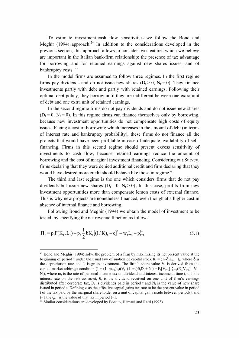
To estimate investment-cash flow sensitivities we follow the Bond and Meghir (1994) approach.24 In addition to the considerations developed in the previous section, this approach allows to consider two features which we believe are important in the Italian bank-firm relationship: the presence of tax advantage for borrowing and for retained earnings against new shares issues, and of bankruptcy costs. 25 In the model firms are assumed to follow three regimes. In the first regime firms pay dividends and do not issue new shares (Dt > 0, Nt = 0). They finance investments partly with debt and partly with retained earnings. Following their optimal debt policy, they borrow until they are indifferent between one extra unit of debt and one extra unit of retained earnings. In the second regime firms do not pay dividends and do not issue new shares (Dt = 0, Nt = 0). In this regime firms can finance themselves only by borrowing, because new investment opportunities do not compensate high costs of equity issues. Facing a cost of borrowing which increases in the amount of debt (in terms of interest rate and bankruptcy probability), these firms do not finance all the projects that would have been profitable in case of adequate availability of self-financing. Firms in this second regime should present excess sensitivity of investments to cash flow, because retained earnings reduce the amount of borrowing and the cost of marginal investment financing. Considering our Survey, firms declaring that they were denied additional credit and firm declaring that they would have desired more credit should behave like those in regime 2. The third and last regime is the one which considers firms that do not pay dividends but issue new shares (Dt = 0, Nt > 0). In this case, profits from new investment opportunities more than compensate lemon costs of external finance. This is why new projects are nonetheless financed, even though at a higher cost in absence of internal finance and borrowing. Following Bond and Meghir (1994) we obtain the model of investment to be tested, by specifying the net revenue function as follows

[ ] tIttt

2ttttttt IpLwc)K/I(bK

21p)L,K(Fp −−−−=Π (5.1)

24 Bond and Meghir (1994) solve the problem of a firm by maximising its net present value at the beginning of period t under the usual law of motion of capital stock Kt = (1–δ)Kt–1+It, where δ is the depreciation rate and It is gross investment. The firm’s share value Vt is derived from the capital market arbitrage condition (1 + (1–mt+1)ιt)(Vt–(1–mt)ϑtDt + Nt) = Et[Vt+1]-ζt+1(Et[Vt+1] –Vt–Nt), where mt is the rate of personal income tax on dividend and interest income at time t, ιt is the interest rate on the riskless asset, θt is the dividend received on one unit of firm’s earnings distributed after corporate tax, Dt is dividends paid in period t and Nt is the value of new share issued in period t. Defining zt as the effective capital gains tax rate to be the present value in period t of the tax paid by the marginal shareholder on a unit of capital gains made between periods t and t+1 the ζt+1 is the value of that tax in period t+1. 25 Similar considerations are developed by Bonato, Hamaui and Ratti (1993).

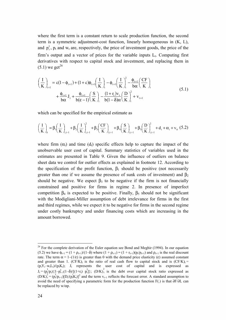
24

where the first term is a constant return to scale production function, the second term is a symmetric adjustment-cost function, linearly homogeneous in (K, L), and I

tp , pt and wt are, respectively, the price of investment goods, the price of the firm’s output and a vector of prices for the variable inputs Lt. Computing first derivatives with respect to capital stock and investment, and replacing them in (5.1) we get26

( ) ( )

( )( )( ) 1t

2

t

tt

t

1tt

1t

t

1t2

t1t

t1t1t

1t

vKD

1bvr1

KS

1bJ

b

KCF

bKI

KIc11c

KI

+++

++++

+

+⎟⎠⎞

⎜⎝⎛

αδ−+−⎟

⎠⎞

⎜⎝⎛

−εφ+

αφ+

⎟⎠⎞

⎜⎝⎛

αφ−⎟

⎠⎞

⎜⎝⎛φ−⎟

⎠⎞

⎜⎝⎛φ++φ−=⎟

⎠⎞

⎜⎝⎛

(5.1)

which can be specified for the empirical estimate as

itit

2

1t,i5

1t,i4

1t,i3

2

1t,i2

1t,i1

itvd

KD

KS

KCF

KI

KI

KI +α++⎟

⎠⎞

⎜⎝⎛β+⎟

⎠⎞

⎜⎝⎛β+⎟

⎠⎞

⎜⎝⎛β+⎟

⎠⎞

⎜⎝⎛β+⎟

⎠⎞

⎜⎝⎛β=⎟

⎠⎞

⎜⎝⎛

−−−−−

(5.2)

where firm (αi) and time (dt) specific effects help to capture the impact of the unobservable user cost of capital. Summary statistics of variables used in the estimates are presented in Table 9. Given the influence of outliers on balance sheet data we control for outlier effects as explained in footnote 12. According to the specification of the profit function, β1 should be positive (not necessarily greater than one if we assume the presence of sunk costs of investment) and β2 should be negative. We espect β3 to be negative if the firm is not financially constrained and positive for firms in regime 2. In presence of imperfect competition β4 is expected to be positive. Finally, β5 should not be significant with the Modigliani-Miller assumption of debt irrelevance for firms in the first and third regimes, while we expect it to be negative for firms in the second regime under costly bankruptcy and under financing costs which are increasing in the amount borrowed.

26 For the complete derivation of the Euler equation see Bond and Meghir (1994). In our equation (5.2) we have φt+1 = (1 + ρt+1)/(1–δ) where (1 + ρt+1) = (1 + rt+1)(pt/pt+1) and ρt+1 is the real discount rate. The term α = 1–(1/ε) is greater than 0 with the demand price elasticity (ε) assumed constant and greater than 1. (CF/K)t is the ratio of real cash flow to capital stock and is (CF/K)t = (ptYt–wtLt)/(ptKt); Jt represents the user cost of capital and is expressed as Jt = (pt

I/pt){1–pIt–1(1–δ)/[(1+rt) pt

I]}; (D/K)2t is the debt over capital stock ratio expressed as

(D/K)2t = (pI

t/pt+1)[Dt/(pitKt)]2 and the term vt+1 reflects the forecast error. A standard assumption to

avoid the need of specifying a parametric form for the production function F(.) is that ∂F/∂L can be replaced by w/αp.

25

6 Results from Euler equation estimations

The specification of firm investment demand presented in (5.3) contains lagged values of the dependent variable among regressors. Considering this Arellano and Bover (1995) and Blundell and Bond (1998) demonstrate that the correlation between the lagged dependent variable and the error term makes OLS estimates biased and inconsistent, even when error terms are not serially correlated. To address this issue the usual approach is that of using ‘first generation’ first-differenced GMM which we also follow to estimate Euler equations in our paper. To estimate equation (5.3) we use the following variables: pS (net sales); piI (total new fixed assets); pCF (cash flow which is operating profit before taxes plus depreciation); D (total debt repayable in more than one year); piK= net capital stock at replacement cost. To calculate piK we use the usual perpetual inventory formula: pt+1Kt+1 = ptKt(1+δt)(pt+1/pt) + pt+1It+1. The depreciation rate is estimated applying the legal depreciation coefficients for land and machinery (land and building share on total capital stock 30% and plants and machinery 70%). Our instruments are two period lagged values of non dummy (or dummy interacted) regressors. In table 10 we present our findings from Euler equation estimation when using self declared credit rationing as subgroup criteria. Diagnostics on these estimates show that residuals are first order, but not second order, autocorrelated and the Sargan test does not reject the null hypothesis of the overall validity of the instruments we use in our estimates.27 Model coefficients in the estimate of the unsorted sample (Table 10, column 1) show the expected signs on cash flow (negative), firm output (positive), debt (negative or insignificant) and on the level (positive) and square (negative) of the investment /capital ratio. A positive and lower than one coefficient for the level of the investment /capital ratio may be interpreted in the logit of the real option hypothesis (Dixit and Pindyck, 1994) (negative c in equation (5.1)) on investment adjustment costs is supported here against the traditional Bond and Meghir (1994) specification in which c is positive. Overall, these findings do not reject the investment choice model proposed by Bond and Meghir (1994). Columns 2, 3 and 4 of Table 10 show that the hypothesis of higher positive sensitivity of investment to cash flow for the subgroups of deniedcred and highlyrationed firms is not rejected. The apparently surprising result on the desirecred subgroup is that the dummy measuring the excess sensitivity of the cash flow coefficient for these firms is significant and negative. This finding may be interpreted as reconciling different perspectives in 27 Exceptions are the two estimates in which we test the cash flow/investment sensitivity of the R&D investing firms and the desirecred subsamples.

26

the financing constraint literature. When the extreme form of financing constraints applies (deniedcred and highlyrationed subgroups), the hypothesis of excess sensitivity of investment to cash flow is not rejected. Under the more generic case of financing constraints (wedge between costs of external and internal finance) the Almeida et al (2004) argument seems to apply and the higher sensitivity of cash reserves and precautionary savings of these firms may generate the result of their (negative) excess sensitivity of investment to cash flow, thereby supporting also KZ findings on this issue. In Table 11 (columns 2, 3, 4 and 5) we use traditional a priori such as size, age, R&D investment status and location in the South as subgroup criteria. In this case we do not find any evidence of higher (positive) sensitivity of investment to cash flow for the subgroup of smaller, younger, R&D investing and located in the South firms. How the overall picture of our results relates to the financing constraints and investment/cash flow sensitivity debate? First, in relation to the FHP argument it seems to show that, on the one hand, a priori criteria are significantly (even though sometimes weakly) correlated to the most extreme forms of financing constraints represented by (self declared) credit rationing. This relationhip holds even after controlling for credit risk measures which are usually not considered in this literature. On the other hand, though, a priori criteria indicated by FHP do not seem to be strong enough, at least in our sample, to become efficient sorting criteria in the identification of subgroups of more financially constrained firms with higher investment/cash flow relationship. Second, our balance sheet/qualitative approach allows to disentangle the observational equivalence problem in the interpretation of the investment/cash flow sensitivity outlined by Alti (2003). In our data we find support for the hypothesis that the investment/cash flow sensitivity is associated to self declared credit rationing and not to the uncertainty about growth prospects of younger firms. Third, our findings are somehow consistent with the KZ hypothesis on the non monotonicity of the investment/cash flow relationship with respect to financing constraints. A priori criteria are shown to be not sufficient to discriminate between subgroups of less (more) financially constrained firms with lower (higher) investment/cash flow sensitivity. In section 2 of the paper, by using the common benchmark in the FHP/KZ debate, we argue that a significant difference in the investment/cash flow sensitivity arises only when we consider the extreme form of financing constraints represented by credit rationing and our findings are consistent with this hypothesis.28 28 GMM estimates for the desirecred subgroups including desirecred firms which are also in the highlyrationed and deniedcred subgroups have also been performed without significant changes in our findings. Results are omitted and available from the authors upon request.

27

7 Conclusions

The missing link of qualitative survey data in which firms directly declare whether they have been credit rationed usually prevents the solution of the controversy among different interpretations of the investment/cash flow sensitivity. In this paper we exploit the opportunity (availability of qualitative survey data) provided by the Capitalia survey database to shed light on this issue. First, we find that standard credit risk measures extracted from previous literature findings, together with ‘discrimination’ variables, significantly affect the probability of self declared credit rationing. The latter include some of the a priori criteria (size, age) used by Fazzari et al (1988 and 2000) to discriminate among subgroups in their test on financing constraints and investment/cash flow sensitivity. Second, we observe that the subgroup of self declared credit rationed firms has excess positive investment/cash flow sensitivity, differently from the complementary subgroup, while this does not occur when we use traditional a priori criteria. Overall, we believe that our findings support the hypothesis that only the credit rationing status may overcome the KZ critique on the non monotonicity between investment-cash flow sensitivity and financing constraints. On their side, a priori criteria appear to be significantly related, in the expected direction, to the probability of credit rationing. Taken as themselves though, they demonstrate to be not enough good predictors of such probability for their successful use in the financing constraint, investment/cash flow literature.

28

References

Abel, A – Eberly, J C (2002) Q theory without adjustment costs & cash flow effects without financing constraints. Mimeo, University of Pennsylvania.

Abel, A – Eberly, J C (2004) Investment, valuation and growth options.

Mimeo, Northwestern University. Almeida, H – Campello, M – Weisbach, M S (2004) The cash flow sensitivity of

cash. Journal of Finance, 59, 4, 1777–1804. Alti, A (2003) How sensitive is investment to cash flow when financing is

frictionless? Journal of Finance, LVIII, 2, 707–722. Altman, E (1968) Financial ratios, discriminant analysis and the prediction of

corporate bankruptcy. Journal of Finance, 23, 589–609. Altman, E (1984) The success of business failure prediction models. An

international survey. Journal of Banking and Finance, 8, 171–198. Altman, E – Baidya, T – Ribeiro Dias, L M (1979) Assessing pPotential

financial problems for firms in Brazil. Journal of International Business Studies, Fall.

Altman, E – Lavallee, M (1981) Business failure classification in Canada.

Journal of Business Administration, Summer. Altman, E – Saunders, A (1998) Credit risk measurement: developments over

the last 20 years. Journal of Banking and Finance, 21, 1721–1742. Arellano, M – Bover, O (1995) Another look at instrumental variables

estimation of the error components model. Journal of Econometrics, 68, 29–51.

Bagella, M – Becchetti, L – Caggese, A (2001) Financing constraints on

investment: a three pillars approach. Research in Economics, 55, 2, 219–254.

Barniv, R – MacDonald, J B (1999) Review of Categorical Models for

Classification Issues in Accounting and Finance. Review of Quantitative Finance and Accounting, 13, 1, 39–62.

29

Beaver, W H (1966) Financial ratios as predictors of failure. Journal of Accounting Research 4, 71–111.

Bianco, M – Jappelli, T – Pagano, M (2005) Courts and banks; effects of

judicial enforcement on credit markets. Journal of Money, Credit and Banking, Vol. 37(2), 223–244.

Bilderbeek, J (1979) An empirical study of the predictive ability of financial

ratios in the Netherlands. Zeitschrift fur Betriebswirtschaft, 5. Blundell, R – Bond, S (1998) Initial conditions and moment restrictions in

dynamic panel data models. Journal of Econometrics, 87, 115–143. Bolton, P – Scharfstein, D S (1996) Optimal debt structure and the number of

creditors. The Journal of Political Economy, 104, 1, 1–25. Bonato, L – Hamaui, R – Ratti, R (1993) Come spiegare la struttura finanziaria

delle imprese italiane. Politica Economica, 9, 49–103. Bond, S – Hoeffler, A – Temple, G (2001) GMM estimations of empirical

growth models. CEPR Discussions Papers n. 3048. Bond, S – Meghir, C (1994) Dynamic investment models and the firm’s

financial policy. The Review of Economic Studies, 61, 197–222. Caggese, A (2004) Testing financing constraints on firm investment using

variable capital. Mimeo, University Pompeu Fabra, Barcellona. Chirinko, R S (1993) Business Fixed Investment Spending. Journal of

Economic Literature, 31, 1875–1911. Cleary, S (1999) The relationship between firm investment and financial

status. Journal of Finance, 54, 673–692. Cole, R A (1998) The importance of relationships to the availability of credit.

Journal of Banking & Finance, Vol. 22, Issue 6–8, 959–977. Detragiache, E – Garella, P – Guiso, L (2000) Multiple versus single banking

relationships: theory and evidence. The Journal of Finance, LV, 3, 1133–1161.

30

Devereaux, M – Schiantarelli, F (1989) Investment, Financial Factors and Cash Flow: evidence from UK Panel Data. NBER Working Paper, No. 3116.

Dixit, A K – Pindyck, R S (1994) Investment under Uncertainty. Princeton

University Press, Princeton, N.J. Dwyer, D – Kocagil, A – Stein, R (2004) The Moody’s KMV RiskCalc v3.1

Model: Next-Generation Technology for Predicting Private Firm Credit Risk. Moody’s KMV.

Edmister, R (1972) An empirical test of financial ratio analysis for small

business failure prediction. Journal of Financial and Quantitative Analysis, 7, 2, 1477–1493.

Fazzari, S M – Hubbard, G R – Petersen, B C (1988) Financing constraints and

corporate investment. Brooking Papers on Economic Activity, 141–195. Fazzari, S M – Hubbard, G R – Petersen, B C (2000) Investment-cash flow

sensitivities are useful: a comment on Kaplan and Zingales. Quarterly Journal of Economics, 115, 2, 695–705.

Focarelli, D – Panetta, F – Salleo, C (2002) Why Do Banks Merge? Journal of

Money, Credit and Banking, 34, 4, 1047–1066. Gertler, M – Hubbard, R G (1988) Financial factors in business fluctuations,

Financial Market Volatility: Causes, consequences and policy recommendations. Federal Reserve Bank of Kansas City, 33–71.

Gilchrist, S – Himmelberg, C P (1995) Evidence on the role of cash flow for

investment. Journal of Monetary Economics, 36, 541–572. Gomes, J F (2001) Financing investment. American Economic Review, 91,

1263–1285. Guiso, L – Sapienza, P – Zingales, L (2004) Does Local Financial Development

Matter? Quarterly Journal of Economics, 119 (3), 929–969. Hayashi, F – Inoue, T (1988) The relation between firm growth and q with

multiple capital goods: theory and evidence from panel data on Japanese firms. Econometrica, 59, 3, 731–753.

31

Hoshi, T – Kashyap, A – Scharfstein, D (1992) Corporate Structure, Liquidity and Investment: Evidence from Japanese Industrial Groups. Quarterly Journal of Economics, 90, 33–61.

Hubbard, G R – Kashyap, A K – Withed, T (1995) Internal finance and firm

investment. Journal of Money Credit and Banking, 27, 683–701. Jappelli, T – Pagano, M (2005) Role and Effects of Credit Information

Sharing. CSEF Working Papers No. 136, Centre for Studies in Economics and Finance (CSEF), University of Salerno, Italy.

Kaplan, S N – Zingales, L (1997) Do investment-cash flow sensitivities provide

useful measures of financing constraints? Quarterly Journal of Economics, 107, 1, 170–215.

Kaplan, S N – Zingales, L (2000) Investment-cash flow sensitivities are not

valid measures of financing constraints. Quarterly Journal of Economics, 115, 2, 707–712.

Keasey, K – McGuinness, P (1990) The failure of UK industrial firms for the

period 1976–1984: logistic analysis and entropy measures. Journal of Business Finance and Accounting, 17, 1, 119–135.

Keasey, K – Watson, R (1991) Financial distress prediction models: a review

of their usefulness. British Journal of Management, 2, 89–102. Ko, C J (1982) A delineation of corporate appraisal models and classification

of bankruptcy firms in Japan. Thesis, New York University. Lo, A W (1986) Logit versus discriminant analysis: a specification test and

application to corporate bankruptcies. Journal of Econometrics, 31, 151–178.

Mattesini, F – Messori, M (2004) L’evoluzione del sistema bancario

meridionale: problemi aperti e possibili soluzioni. Il Mulino, Bologna. Moyen, N (2004) Investment – cash flow sensitivities: constrained versus

unconstrained firms. The Journal of Finance, 59, 5, 2061–2092. Neyman, J (1934) On the two different aspects of the representative method:

the method of stratified sampling and the method of purposive selection. Journal of the Royal Statistical Society B, 97, 558–606.

32

Ohlson, J A (1980) Financial ratios and the probabilistic prediction of bankruptcy. Journal of Accounting Research, 18, 109–131.

Pavitt, K (1984) Sectoral patterns of technological change: Towards a

taxonomy and a theory. Research Policy, 13, 4, 343–373. Petersen, M – Rajan, R (1994) The benefits of lending relationships: evidence

from small business data. Journal of Finance, 49, 1367–1400. Saretto, A A (2004) Predicting and pricing the probability of default. Working

Paper, UCLA. Sapienza, P (2002) The effect of banking mergers on loan contracts. The

Journal of Finance, Vol. 57, No. 1, 329–367. Schiantarelli, F – Georgoutsos, D (1990) Imperfect competition, Tobin’s q and

investment: evidence from aggregate UK data. European Economic Review, 34, 1061–1078.

Schiantarelli, F (1996) Financial constraints and investment: methodological

issues and international evidence. Oxford Review of Economic Policy, 12, 2, 70–89.

Shumway, T (2001) Forecasting bankruptcy more accurately: a simple hazard

rate model. Journal of Business, 74, 101–124. Skogsvik, K (1990) Current cost accounting ratios as predictors of business

failure: the Swedish case. Journal of Business Finance & Accounting, 17, 1, 137–160.

van Frederkslust, R (1978) Predictability of corporate failure. Martinus Nijhoff

Social Science Division, Leiden. von Thadden, E L (1995) Long term contracts, short term investment and

monitoring. Review of Economic Studies, 62, 557–575. Whited, T M (1992) Debt, Liquidity Constraints, and Corporate Investment:

Evidence from Panel Data. The Journal of Finance, 47, 1425–1460. Zavgren, C V (1985) Assessing the vulnerability to failure of American

industrial firms: a logistic analysis. Journal of Business Finance & Accounting, 12, 1, 19–45.

33

Zmijeski, M E (1984) Methodological issues related to the estimation of financial distress prediction models. Journal of Accounting Research, 22, supplement, 59–82.

34

Table 1. Descriptive features of the Capitalia sample (size breakdown) Our sample includes 3,840 firms. Firms are grouped by average number of employees in the period 1998–2000. Small firms are those with less than 50 employees, medium firms are those with less (more) than 250 (50) employees, large firms are those with more than 250 employees. Pavitt is sector classification as defined by Pavitt. Macroareas: North West, North East, Central Regionsa and South and Isles. Group, Susidy, R&D and Export are the % of firms that respectively belong to a group, have been subsidised, have invested in R&D and export part of their production. Age is the difference between 2001 and firm's year of birth. Number of banks is the number of banks with which the firm has commercial relationships. Debt share is the share of the overall bank debt held by the main lender. Local bank means that the main lender is located in the same province. Duration is the length in years of the main bank relationship. Small Medium Large traditional 55.30 43.77 40.82

Pavitt scale economies 18.51 15.08 23.67 specialised 22.38 32.30 28.16

high tech 3.80 8.85 7.35 north west 35.32 43.11 44.90

Macroareas north east 26.98 29.51 37.14 central regions 23.18 14.10 12.24

south & isles 14.51 13.28 5.71 Group 12.07 31.58 84.43 Subsidy 38.27 56.03 60.50 R&D 31.11 57.00 76.67 Export 63.51 86.84 93.88 Age 23.24* 30.30* 38.66* Number of banks 4.46 7.13 10.51 Debt share 41.10 34.76 19.31 Local bank 65.39 57.65 47.47 Duration 17.02* 19.31* 19.12*

Percentage values except * which are averages.

35

Table 2a. Identity features of the Capitalia sample (credit rationing breakdown) Our sample includes 3,840 firms. Firms are grouped by intensity of financing constraints. Total weight is the percentage of firms belonging to the desirecred, deniedcred and highlyrationed group (for group definitions see section 3.2). Size is the average number of employees in the period 1998–2000. Age is the difference between 2001 and firm's year birth. Number of banks is the number of banks with which the firm has commercial relationships in the considered period. Debt share is the share of the overall bank debt held by the main lender.

All Desirected Deniedcred Highlyrationed Total weight yes no yes no yes no 18.42 81.58 4.62 95.38 1.97 98.03 mean 7784 43.17 74.41 56.78 68.57 46.84 78.46

Size median 22.00 20.00 22.33 20.67 21.67 20.33 22.00 sd 283.90 82.89 264.07 145.72 245.57 98.21 286.38

obs. 3853 696 3083 170 3507 76 3777 mean 25.34 23.74 25.39 24.22 25.11 21.55 25.42

Age median 21.00 19.00 21.00 18.00 21.00 18.50 21.00 sd 18.51 19.81 17.63 20.75 17.93 16.58 18.54

obs. 3853 696 3083 170 3507 76 3777 mean 5.23 5.34 5.21 5.82 5.17 5.43 5.23

Number of banks median 4.00 4.00 4.00 5.00 4.00 4.00 4.00 sd 3.69 3.59 3.69 4.09 3.62 3.91 3.68

obs. 3806 695 3072 169 3497 75 3731 mean 39.53 40.86 39.17 41.92 39.44 43.15 39.45

Debt share median 30.00 40.00 30.00 40.00 30.00 40.00 30.00 sd 24.08 22.02 24.61 23.77 24.06 24.09 24.08

obs 2666 554 2094 138 2433 61 2605

36

Table 2b. Identity features of the Capitalia sample (credit rationing breakdown) Our sample includes 3,840 firms. Firms are grouped by intensity of financing constraints. Size classes: small, medium and large are firms with respectively less than 50, between 50 and 250 and more than 250 employees. Macroareas: North West, North East, Central Regions, South and Isles. Art. 18 refers to the Italian Law 300/1975 increasing firing costs for firms with more than fifteen workers (footnote 14 in the paper). Share of debt is the share of the overall bank debt held by the main lender. Main financing by bank debt, Local bank, Export, Group, Subsidy and R&D are the percent of firms that respectively have financed their investments mainly with bank debt, whose main lender is located in the same province, export part of their production, belong to a group, have been subsidised and have invested in R&D.

All Desirected Deniedcred Highlyrationed yes no yes no yes no small 77.81 83.91 77.33 82.35 78.87 81.58 77.73

Size Classes medium 15.83 13.22 16.7 12.94 15.74 14.47 15.86 large 6.36 2.87 5.97 4.71 5.39 3.95 6.41

all 100 100 100 100 100 100 100 north west 37.17 33.48 37.69 35.29 36.7 28.95 37.33 north east 28.03 21.26 29.58 17.65 28.69 13.16 28.33 Macroareas central regions 21.05 23.42 20.76 24.71 21.04 32.89 20.81 south & isles 13.76 21.84 11.97 22.35 13.57 25 13.53 all 100 100 100 100 100 100 100 more than 15 73.6 69.68 74.28 68.82 73.2 64.47 73.79 Art. 18 less than 15 26.4 30.32 25.72 31.18 26.8 35.53 26.21 all 100 100 100 100 100 100 100 < 20% 18.53 17.67 19.07 18.82 18.73 17.11 18.56

Debt Share > 20% and < 50% 34.44 42.24 33.18 39.41 34.42 38.16 34.37 > 50% 47.03 40.09 47.75 41.76 46.85 44.74 47.07

all 100 100 100 100 100 100 100

Main fin. by bank debt

yes 12.31 15.41 11.76 18.79 12.23 14.29 12.27 no 87.69 84.59 88.24 81.21 87.77 85.71 87.73 all 100 100 100 100 100 100 100

yes 63.19 66.32 62.59 66.06 63.21 60 63.26 Local bank no 36.81 33.68 37.41 33.94 36.79 40 36.74 all 100 100 100 100 100 100 100 yes 69.14 66.04 69.52 66.47 68.76 63.16 69.26 Export no 30.86 33.96 30.48 33.53 31.24 36.84 30.74 all 100 100 100 100 100 100 100 yes 19.75 16.09 19.58 17.06 18.92 17.11 19.8 Group no 80.25 83.91 80.42 82.94 81.08 82.89 80.2 all 100 100 100 100 100 100 100 yes 42.45 43.17 42.51 40.59 42.35 42.11 42.46 Subsidy no 57.55 56.83 57.49 59.41 57.65 57.89 57.54 all 100 100 100 100 100 100 100 yes 38.09 37.03 37.88 41.42 37.58 43.42 37.98 R&D no 61.91 62.97 62.12 58.58 62.42 56.58 62.02 all 100 100 100 100 100 100 100

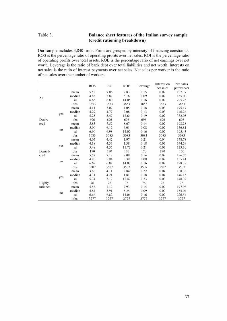
37

Table 3. Balance sheet features of the Italian survey sample (credit rationing breakdown) Our sample includes 3,840 firms. Firms are grouped by intensity of financing constraints. ROS is the percentage ratio of operating profits over net sales. ROI is the percentage ratio of operating profits over total assets. ROE is the percentage ratio of net earnings over net worth. Leverage is the ratio of bank debt over total liabilities and net worth. Interests on net sales is the ratio of interest payments over net sales. Net sales per worker is the ratio of net sales over the number of workers. ROS ROI ROE Leverage Interest on

net sales Net sales

per worker

All

mean 5.52 7.06 7.83 0.15 0.02 197.77 median 4.83 5.87 5.16 0.09 0.02 155.00 sd 6.65 6.80 14.05 0.16 0.02 225.25 obs 3853 3853 3853 3853 3853 3853

Desire-cred

yes

mean 4.11 5.07 4.05 0.18 0.03 195.17 median 4.29 4.77 2.08 0.13 0.03 146.26

sd 5.25 5.47 13.64 0.19 0.02 332.05 obs 696 696 696 696 696 696

no

mean 5.83 7.52 8.67 0.14 0.02 198.28 median 5.00 6.12 6.01 0.08 0.02 156.81

sd 6.90 6.98 14.02 0.16 0.02 195.43 obs 3083 3083 3083 3083 3083 3083

Denied-cred

yes

mean 4.05 4.42 1.97 0.21 0.04 178.78 median 4.18 4.33 1.38 0.18 0.03 144.59

sd 5.48 4.55 11.72 0.21 0.03 123.10 obs 170 170 170 170 170 170

no

mean 5.57 7.18 8.09 0.14 0.02 196.76 median 4.85 5.94 5.39 0.08 0.02 155.41

sd 6.69 6.82 14.07 0.16 0.02 198.38 obs 3507 3507 3507 3507 3507 3507

Highly-rationed

yes

mean 3.86 4.11 2.84 0.22 0.04 188.38 median 4.31 4.21 1.81 0.18 0.04 146.15

sd 5.74 5.17 12.47 0.23 0.03 148.39 obs 76 76 76 76 76 76

no

mean 5.56 7.12 7.93 0.15 0.02 197.96 median 4.84 5.91 5.25 0.09 0.02 155.04

sd 6.66 6.82 14.06 0.16 0.02 226.54 obs 3777 3777 3777 3777 3777 3777

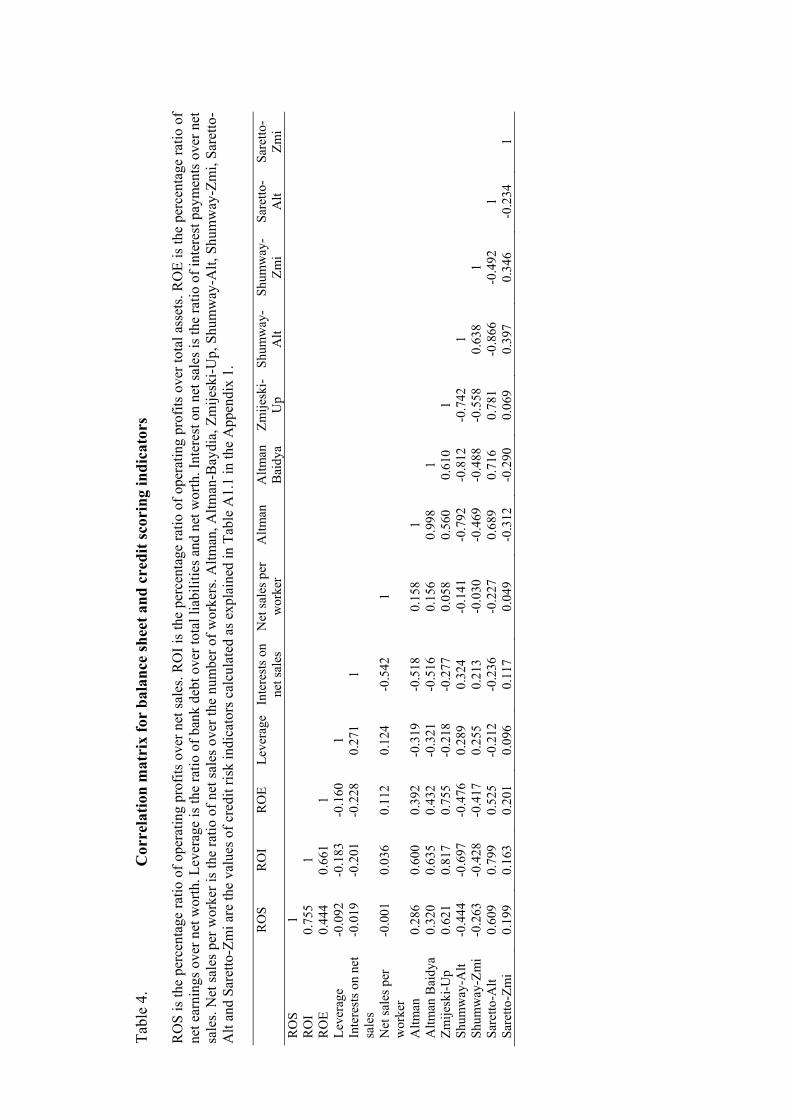
Tabl

e 4.

C

orre

latio

n m

atri

x fo

r ba

lanc

e sh

eet a

nd c

redi

t sco

ring

indi

cato

rs

RO

S is

the

perc

enta

ge ra

tio o

f ope

ratin

g pr

ofits

ove

r net

sal

es. R

OI i

s th

e pe

rcen

tage

ratio

of o

pera

ting

prof

its o

ver t

otal

ass

ets.

RO

E is

the

perc

enta

ge ra

tio o

f ne

t ear

ning

s ove

r net

wor

th. L

ever

age

is th

e ra

tio o

f ban

k de

bt o

ver t

otal

liab

ilitie

s and

net

wor

th. I

nter

est o

n ne

t sal

es is

the

ratio

of i

nter

est p

aym

ents

ove

r net

sa

les.

Net

sal

es p

er w

orke

r is

the

ratio

of n

et s

ales

ove

r the

num

ber o

f wor

kers

. Altm

an, A

ltman

-Bay

dia,

Zm

ijesk

i-Up,

Shu

mw

ay-A

lt, S

hum

way

-Zm

i, Sa

retto

-A

lt an

d Sa

retto

-Zm

i are

the

valu

es o

f cre

dit r

isk

indi

cato

rs c

alcu

late

d as

exp

lain

ed in

Tab

le A

1.1

in th

e A

ppen

dix

1.

R

OS

RO

I R

OE

Leve

rage

Inte

rest

s on

net s

ales

N

et sa

les p

er

wor

ker

Altm

an

Altm

an

Bai

dya

Zmije

ski-

Up

Shum

way

-A

lt Sh

umw

ay-

Zmi

Sare

tto-

Alt

Sare

tto-

Zmi

RO

S 1

RO

I 0.

755

1

RO

E 0.

444

0.66

1 1

Leve

rage

-0

.092

-0

.183

-0

.160

1

In

tere

sts o

n ne

t sa

les

-0.0

19

-0.2

01

-0.2

28

0.27

1 1

Net

sale

s per

w

orke

r -0

.001

0.

036

0.11

2 0.

124

-0.5

42

1

Altm

an

0.28

6 0.

600

0.39

2 -0

.319

-0

.518

0.

158

1

A

ltman

Bai

dya

0.32

0 0.

635

0.43

2 -0

.321

-0

.516

0.

156

0.99

8 1

Zm

ijesk

i-Up

0.62

1 0.

817

0.75

5 -0

.218

-0

.277

0.

058

0.56

0 0.

610

1

Sh

umw

ay-A

lt -0

.444

-0

.697

-0

.476

0.

289

0.32

4 -0

.141

-0

.792

-0

.812

-0

.742

1

Sh

umw

ay-Z

mi

-0.2

63

-0.4

28

-0.4

17

0.25

5 0.

213

-0.0

30

-0.4

69

-0.4

88

-0.5

58

0.63

8 1

Sare

tto-A

lt 0.

609

0.79

9 0.

525

-0.2

12

-0.2

36

-0.2

27

0.68

9 0.

716

0.78

1 -0

.866

-0

.492

1

Sa

retto

-Zm

i 0.

199

0.16

3 0.

201

0.09

6 0.

117

0.04

9 -0

.312

-0

.290

0.

069

0.39

7 0.

346

-0.2

34

1

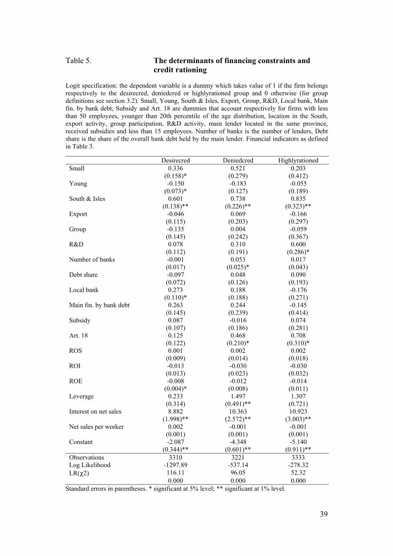
39

Table 5. The determinants of financing constraints and credit rationing Logit specification: the dependent variable is a dummy which takes value of 1 if the firm belongs respectively to the desirecred, deniedcred or highlyrationed group and 0 otherwise (for group definitions see section 3.2). Small, Young, South & Isles, Export, Group, R&D, Local bank, Main fin. by bank debt, Subsidy and Art. 18 are dummies that account respectively for firms with less than 50 employees, younger than 20th percentile of the age distribution, location in the South, export activity, group participation, R&D activity, main lender located in the same province, received subsidies and less than 15 employees. Number of banks is the number of lenders, Debt share is the share of the overall bank debt held by the main lender. Financial indicators as defined in Table 3.

Desirecred Deniedcred Highlyrationed Small 0.336 0.521 0.203 (0.158)* (0.279) (0.412) Young -0.150 -0.183 -0.055 (0.073)* (0.127) (0.189) South & Isles 0.601 0.738 0.835 (0.138)** (0.226)** (0.323)** Export -0.046 0.069 -0.166 (0.115) (0.203) (0.297) Group -0.135 0.004 -0.059 (0.145) (0.242) (0.367) R&D 0.078 0.310 0.600 (0.112) (0.191) (0.286)* Number of banks -0.001 0.053 0.017 (0.017) (0.025)* (0.043) Debt share -0.097 0.048 0.090 (0.072) (0.126) (0.193) Local bank 0.273 0.188 -0.176 (0.110)* (0.188) (0.271) Main fin. by bank debt 0.263 0.244 -0.145 (0.145) (0.239) (0.414) Subsidy 0.087 -0.016 0.074 (0.107) (0.186) (0.281) Art. 18 0.125 0.468 0.708 (0.122) (0.210)* (0.310)* ROS 0.001 0.002 0.002 (0.009) (0.014) (0.018) ROI -0.013 -0.030 -0.030 (0.013) (0.023) (0.032) ROE -0.008 -0.012 -0.014 (0.004)* (0.008) (0.011) Leverage 0.233 1.497 1.307 (0.314) (0.491)** (0.721) Interest on net sales 8.882 10.363 10.923 (1.998)** (2.572)** (3.003)** Net sales per worker 0.002 -0.001 -0.001 (0.001) (0.001) (0.001) Constant -2.087 -4.348 -5.140 (0.344)** (0.601)** (0.911)** Observations 3310 3221 3333 Log Likelihood -1297.89 -537.14 -278.32 LR(χ2) 116.11 96.05 52.32 0.000 0.000 0.000

Standard errors in parentheses. * significant at 5% level; ** significant at 1% level.

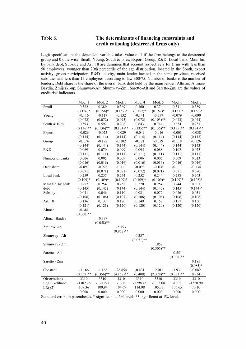
40

Table 6. The determinants of financing constraints and credit rationing (desirecred firms only) Logit specification: the dependent variable takes value of 1 if the firm belongs to the desirecred group and 0 otherwise. Small, Young, South & Isles, Export, Group, R&D, Local bank, Main fin. by bank debt, Subsidy and Art. 18 are dummies that account respectively for firms with less than 50 employees, younger than 20th percentile of the age distribution, located in the South, export activity, group participation, R&D activity, main lender located in the same province, received subsidies and less than 15 employees according to law 300/75. Number of banks is the number of lenders, Debt share is the share of the overall bank debt held by the main lender. Altman, Altman-Baydia, Zmijeski-up, Shumway-Alt, Shumway-Zmi, Saretto-Alt and Saretto-Zmi are the values of credit risk indicators.

Mod. 1 Mod. 2 Mod. 3 Mod. 4 Mod. 5 Mod. 6 Mod. 7 Small 0.382 0.380 0.369 0.360 0.374 0.341 0.389 (0.156)* (0.156)* (0.157)* (0.157)* (0.157)* (0.157)* (0.156)* Young -0.116 -0.117 -0.132 -0.141 -0.557 -0.079 -0.090 (0.072) (0.072) (0.073) (0.072) (0.103)** (0.073) (0.074) South & Isles 0.593 0.592 0.706 0.643 0.744 0.654 0.751 (0.136)** (0.136)** (0.134)** (0.135)** (0.135)** (0.135)** (0.134)** Export -0.026 -0.025 -0.029 -0.049 -0.016 -0.003 -0.038 (0.114) (0.114) (0.114) (0.114) (0.114) (0.114) (0.113) Group -0.174 -0.172 -0.102 -0.121 -0.079 -0.118 -0.126 (0.144) (0.144) (0.144) (0.144) (0.144) (0.144) (0.143) R&D 0.069 0.070 0.099 0.095 0.088 0.102 0.075 (0.111) (0.111) (0.111) (0.111) (0.111) (0.111) (0.111) Number of banks 0.006 0.005 0.009 0.006 0.005 0.009 0.013 (0.016) (0.016) (0.016) (0.016) (0.016) (0.016) (0.016) Debt share -0.097 -0.096 -0.111 -0.096 -0.106 -0.111 -0.134 (0.071) (0.071) (0.071) (0.072) (0.071) (0.071) (0.070) Local bank 0.259 0.257 0.244 0.252 0.244 0.258 0.263 (0.109)* (0.109)* (0.109)* (0.109)* (0.109)* (0.109)* (0.108)* Main fin. by bank 0.257 0.254 0.258 0.220 0.254 0.244 0.301 debt (0.145) (0.145) (0.144) (0.144) (0.145) (0.145) (0.144)* Subsidy 0.041 0.046 0.110 0.081 0.072 0.076 0.031 (0.106) (0.106) (0.107) (0.106) (0.106) (0.106) (0.106) Art. 18 0.136 0.137 0.170 0.149 0.157 0.157 0.150 (0.121) (0.121) (0.120) (0.120) (0.120) (0.120) (0.120) Altman -0.381 (0.060)** Altman-Baidya -0.377 (0.058)** Zmijeski-up -5.753 (0.958)** Shumway - Alt 0.337 (0.051)** Shumway - Zmi 1.852 (0.305)** Saretto - Alt -0.551 (0.088)** Saretto - Zmi 0.185 (0.083)* Constant -1.166 -1.166 -26.854 -0.431 12.016 -1.931 -0.082 (0.357)** (0.356)** (4.157)** (0.408) (2.328)** (0.333)** (0.934) Observations 3310 3310 3310 3310 3310 3310 3310 Log Likelihood -1302.26 -1300.97 -1303 -1298.45 -1303.08 -1302 -1320.90 LR(χ2) 107.36 109.94 104.69 114.98 105.73 106.65 70.10 0.000 0.000 0.000 0.000 0.000 0.000 0.000

Standard errors in parentheses. * significant at 5% level; ** significant at 1% level.

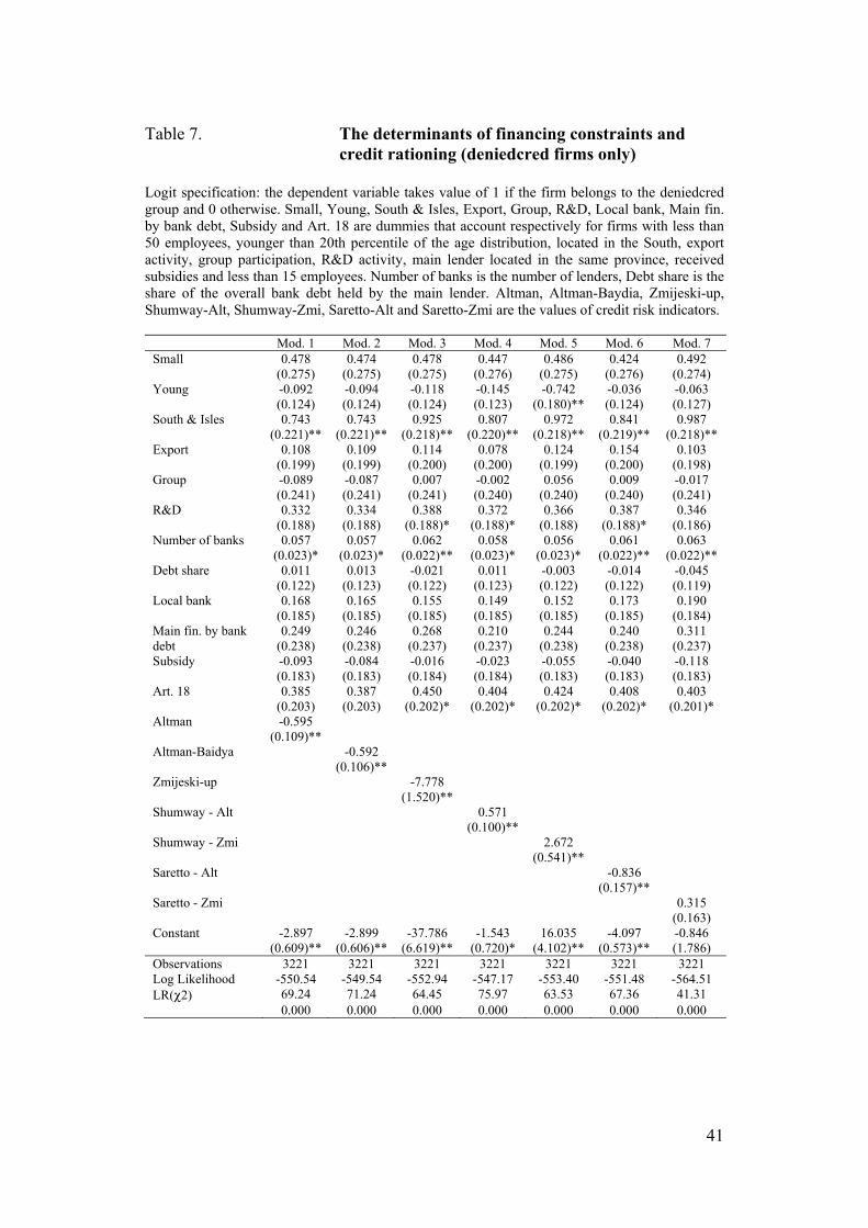
41

Table 7. The determinants of financing constraints and credit rationing (deniedcred firms only) Logit specification: the dependent variable takes value of 1 if the firm belongs to the deniedcred group and 0 otherwise. Small, Young, South & Isles, Export, Group, R&D, Local bank, Main fin. by bank debt, Subsidy and Art. 18 are dummies that account respectively for firms with less than 50 employees, younger than 20th percentile of the age distribution, located in the South, export activity, group participation, R&D activity, main lender located in the same province, received subsidies and less than 15 employees. Number of banks is the number of lenders, Debt share is the share of the overall bank debt held by the main lender. Altman, Altman-Baydia, Zmijeski-up, Shumway-Alt, Shumway-Zmi, Saretto-Alt and Saretto-Zmi are the values of credit risk indicators.

Mod. 1 Mod. 2 Mod. 3 Mod. 4 Mod. 5 Mod. 6 Mod. 7 Small 0.478 0.474 0.478 0.447 0.486 0.424 0.492 (0.275) (0.275) (0.275) (0.276) (0.275) (0.276) (0.274) Young -0.092 -0.094 -0.118 -0.145 -0.742 -0.036 -0.063 (0.124) (0.124) (0.124) (0.123) (0.180)** (0.124) (0.127) South & Isles 0.743 0.743 0.925 0.807 0.972 0.841 0.987 (0.221)** (0.221)** (0.218)** (0.220)** (0.218)** (0.219)** (0.218)** Export 0.108 0.109 0.114 0.078 0.124 0.154 0.103 (0.199) (0.199) (0.200) (0.200) (0.199) (0.200) (0.198) Group -0.089 -0.087 0.007 -0.002 0.056 0.009 -0.017 (0.241) (0.241) (0.241) (0.240) (0.240) (0.240) (0.241) R&D 0.332 0.334 0.388 0.372 0.366 0.387 0.346 (0.188) (0.188) (0.188)* (0.188)* (0.188) (0.188)* (0.186) Number of banks 0.057 0.057 0.062 0.058 0.056 0.061 0.063 (0.023)* (0.023)* (0.022)** (0.023)* (0.023)* (0.022)** (0.022)** Debt share 0.011 0.013 -0.021 0.011 -0.003 -0.014 -0.045 (0.122) (0.123) (0.122) (0.123) (0.122) (0.122) (0.119) Local bank 0.168 0.165 0.155 0.149 0.152 0.173 0.190 (0.185) (0.185) (0.185) (0.185) (0.185) (0.185) (0.184) Main fin. by bank 0.249 0.246 0.268 0.210 0.244 0.240 0.311 debt (0.238) (0.238) (0.237) (0.237) (0.238) (0.238) (0.237) Subsidy -0.093 -0.084 -0.016 -0.023 -0.055 -0.040 -0.118 (0.183) (0.183) (0.184) (0.184) (0.183) (0.183) (0.183) Art. 18 0.385 0.387 0.450 0.404 0.424 0.408 0.403 (0.203) (0.203) (0.202)* (0.202)* (0.202)* (0.202)* (0.201)* Altman -0.595 (0.109)** Altman-Baidya -0.592 (0.106)** Zmijeski-up -7.778 (1.520)** Shumway - Alt 0.571 (0.100)** Shumway - Zmi 2.672 (0.541)** Saretto - Alt -0.836 (0.157)** Saretto - Zmi 0.315 (0.163) Constant -2.897 -2.899 -37.786 -1.543 16.035 -4.097 -0.846 (0.609)** (0.606)** (6.619)** (0.720)* (4.102)** (0.573)** (1.786) Observations 3221 3221 3221 3221 3221 3221 3221 Log Likelihood -550.54 -549.54 -552.94 -547.17 -553.40 -551.48 -564.51 LR(χ2) 69.24 71.24 64.45 75.97 63.53 67.36 41.31 0.000 0.000 0.000 0.000 0.000 0.000 0.000

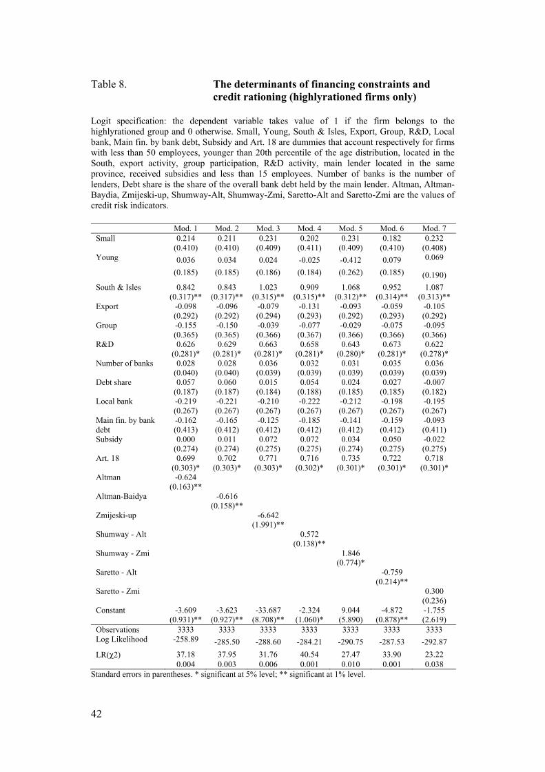
42

Table 8. The determinants of financing constraints and credit rationing (highlyrationed firms only) Logit specification: the dependent variable takes value of 1 if the firm belongs to the highlyrationed group and 0 otherwise. Small, Young, South & Isles, Export, Group, R&D, Local bank, Main fin. by bank debt, Subsidy and Art. 18 are dummies that account respectively for firms with less than 50 employees, younger than 20th percentile of the age distribution, located in the South, export activity, group participation, R&D activity, main lender located in the same province, received subsidies and less than 15 employees. Number of banks is the number of lenders, Debt share is the share of the overall bank debt held by the main lender. Altman, Altman-Baydia, Zmijeski-up, Shumway-Alt, Shumway-Zmi, Saretto-Alt and Saretto-Zmi are the values of credit risk indicators.

Mod. 1 Mod. 2 Mod. 3 Mod. 4 Mod. 5 Mod. 6 Mod. 7 Small 0.214 0.211 0.231 0.202 0.231 0.182 0.232 (0.410) (0.410) (0.409) (0.411) (0.409) (0.410) (0.408) Young 0.036 0.034 0.024 -0.025 -0.412 0.079 0.069

(0.185) (0.185) (0.186) (0.184) (0.262) (0.185) (0.190) South & Isles 0.842 0.843 1.023 0.909 1.068 0.952 1.087 (0.317)** (0.317)** (0.315)** (0.315)** (0.312)** (0.314)** (0.313)** Export -0.098 -0.096 -0.079 -0.131 -0.093 -0.059 -0.105 (0.292) (0.292) (0.294) (0.293) (0.292) (0.293) (0.292) Group -0.155 -0.150 -0.039 -0.077 -0.029 -0.075 -0.095 (0.365) (0.365) (0.366) (0.367) (0.366) (0.366) (0.366) R&D 0.626 0.629 0.663 0.658 0.643 0.673 0.622 (0.281)* (0.281)* (0.281)* (0.281)* (0.280)* (0.281)* (0.278)* Number of banks 0.028 0.028 0.036 0.032 0.031 0.035 0.036 (0.040) (0.040) (0.039) (0.039) (0.039) (0.039) (0.039) Debt share 0.057 0.060 0.015 0.054 0.024 0.027 -0.007 (0.187) (0.187) (0.184) (0.188) (0.185) (0.185) (0.182) Local bank -0.219 -0.221 -0.210 -0.222 -0.212 -0.198 -0.195 (0.267) (0.267) (0.267) (0.267) (0.267) (0.267) (0.267) Main fin. by bank -0.162 -0.165 -0.125 -0.185 -0.141 -0.159 -0.093 debt (0.413) (0.412) (0.412) (0.412) (0.412) (0.412) (0.411) Subsidy 0.000 0.011 0.072 0.072 0.034 0.050 -0.022 (0.274) (0.274) (0.275) (0.275) (0.274) (0.275) (0.275) Art. 18 0.699 0.702 0.771 0.716 0.735 0.722 0.718 (0.303)* (0.303)* (0.303)* (0.302)* (0.301)* (0.301)* (0.301)* Altman -0.624 (0.163)** Altman-Baidya -0.616 (0.158)** Zmijeski-up -6.642 (1.991)** Shumway - Alt 0.572 (0.138)** Shumway - Zmi 1.846 (0.774)* Saretto - Alt -0.759 (0.214)** Saretto - Zmi 0.300 (0.236) Constant -3.609 -3.623 -33.687 -2.324 9.044 -4.872 -1.755 (0.931)** (0.927)** (8.708)** (1.060)* (5.890) (0.878)** (2.619) Observations 3333 3333 3333 3333 3333 3333 3333 Log Likelihood -258.89 -285.50 -288.60 -284.21 -290.75 -287.53 -292.87 LR(χ2) 37.18 37.95 31.76 40.54 27.47 33.90 23.22 0.004 0.003 0.006 0.001 0.010 0.001 0.038

Standard errors in parentheses. * significant at 5% level; ** significant at 1% level.

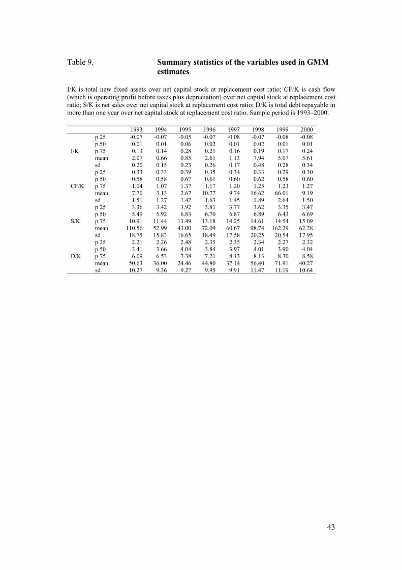
43

Table 9. Summary statistics of the variables used in GMM estimates I/K is total new fixed assets over net capital stock at replacement cost ratio; CF/K is cash flow (which is operating profit before taxes plus depreciation) over net capital stock at replacement cost ratio; S/K is net sales over net capital stock at replacement cost ratio; D/K is total debt repayable in more than one year over net capital stock at replacement cost ratio. Sample period is 1993–2000.

1993 1994 1995 1996 1997 1998 1999 2000

I/K

p 25 -0.07 -0.07 -0.05 -0.07 -0.08 -0.07 -0.08 -0.08 p 50 0.01 0.01 0.06 0.02 0.01 0.02 0.01 0.01 p 75 0.13 0.14 0.28 0.21 0.16 0.19 0.17 0.24 mean 2.07 0.66 0.85 2.61 1.13 7.94 5.07 5.61 sd 0.20 0.15 0.23 0.26 0.17 0.48 0.28 0.34

CF/K

p 25 0.33 0.33 0.39 0.35 0.34 0.33 0.29 0.30 p 50 0.58 0.58 0.67 0.61 0.60 0.62 0.58 0.60 p 75 1.04 1.07 1.37 1.17 1.20 1.25 1.23 1.27 mean 7.70 3.13 2.67 10.77 9.74 16.62 66.01 9.19 sd 1.51 1.27 1.42 1.63 1.45 1.89 2.64 1.50

S/K

p 25 3.36 3.42 3.92 3.81 3.77 3.62 3.35 3.47 p 50 5.49 5.92 6.83 6.70 6.87 6.89 6.43 6.69 p 75 10.91 11.44 13.49 13.18 14.25 14.61 14.54 15.09 mean 110.56 52.99 43.00 72.09 60.67 98.74 162.29 62.28 sd 18.75 15.83 16.65 18.49 17.58 20.25 20.54 17.95

D/K

p 25 2.21 2.26 2.48 2.35 2.35 2.34 2.27 2.32 p 50 3.41 3.66 4.04 3.84 3.97 4.01 3.90 4.04 p 75 6.09 6.53 7.38 7.21 8.13 8.13 8.30 8.58 mean 50.63 36.00 24.46 44.80 37.14 56.40 71.91 40.27 sd 10.27 9.36 9.27 9.95 9.91 11.47 11.19 10.64

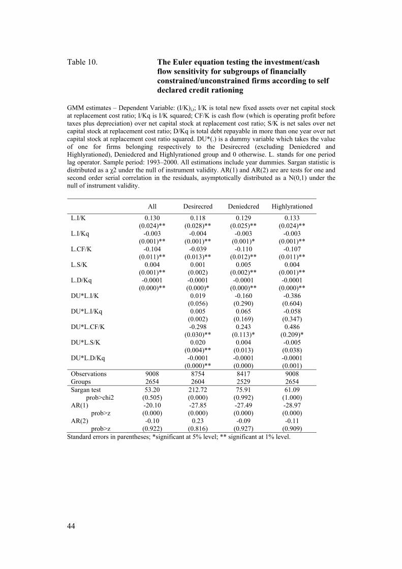
44

Table 10. The Euler equation testing the investment/cash flow sensitivity for subgroups of financially constrained/unconstrained firms according to self declared credit rationing GMM estimates – Dependent Variable: (I/K)i,t; I/K is total new fixed assets over net capital stock at replacement cost ratio; I/Kq is I/K squared; CF/K is cash flow (which is operating profit before taxes plus depreciation) over net capital stock at replacement cost ratio; S/K is net sales over net capital stock at replacement cost ratio; D/Kq is total debt repayable in more than one year over net capital stock at replacement cost ratio squared. DU*(.) is a dummy variable which takes the value of one for firms belonging respectively to the Desirecred (excluding Deniedcred and Highlyrationed), Deniedcred and Highlyrationed group and 0 otherwise. L. stands for one period lag operator. Sample period: 1993–2000. All estimations include year dummies. Sargan statistic is distributed as a χ2 under the null of instrument validity. AR(1) and AR(2) are are tests for one and second order serial correlation in the residuals, asymptotically distributed as a N(0,1) under the null of instrument validity.

All Desirecred Deniedcred Highlyrationed

L.I/K 0.130 0.118 0.129 0.133 (0.024)** (0.028)** (0.025)** (0.024)** L.I/Kq -0.003 -0.004 -0.003 -0.003 (0.001)** (0.001)** (0.001)* (0.001)** L.CF/K -0.104 -0.039 -0.110 -0.107 (0.011)** (0.013)** (0.012)** (0.011)** L.S/K 0.004 0.001 0.005 0.004 (0.001)** (0.002) (0.002)** (0.001)** L.D/Kq -0.0001 -0.0001 -0.0001 -0.0001 (0.000)** (0.000)* (0.000)** (0.000)** DU*L.I/K 0.019 -0.160 -0.386 (0.056) (0.290) (0.604) DU*L.I/Kq 0.005 0.065 -0.058 (0.002) (0.169) (0.347) DU*L.CF/K -0.298 0.243 0.486 (0.030)** (0.113)* (0.209)* DU*L.S/K 0.020 0.004 -0.005 (0.004)** (0.013) (0.038) DU*L.D/Kq -0.0001 -0.0001 -0.0001 (0.000)** (0.000) (0.001) Observations 9008 8754 8417 9008 Groups 2654 2604 2529 2654 Sargan test 53.20 212.72 75.91 61.09 prob>chi2 (0.505) (0.000) (0.992) (1.000) AR(1) -20.10 -27.85 -27.49 -28.97 prob>z (0.000) (0.000) (0.000) (0.000) AR(2) -0.10 0.23 -0.09 -0.11 prob>z (0.922) (0.816) (0.927) (0.909)

Standard errors in parentheses; *significant at 5% level; ** significant at 1% level.

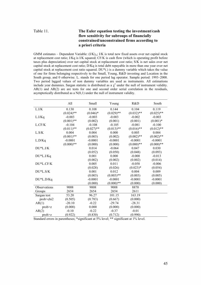
45

Table 11. The Euler equation testing the investment/cash flow sensitivity for subroups of financially constrained/unconstrained firms according to a priori criteria GMM estimates – Dependent Variable: (I/K)i,t; I/K is total new fixed assets over net capital stock at replacement cost ratio; I/Kq is I/K squared; CF/K is cash flow (which is operating profit before taxes plus depreciation) over net capital stock at replacement cost ratio; S/K is net sales over net capital stock at replacement cost ratio; D/Kq is total debt repayable in more than one year over net capital stock at replacement cost ratio squared. DU*(.) is a dummy variable which takes the value of one for firms belonging respectively to the Small, Young, R&D investing and Location in the South group, and 0 otherwise. L. stands for one period lag operator. Sample period: 1993–2000. Two period lagged values of non dummy variables are used as instruments. All estimations include year dummies. Sargan statistic is distributed as a χ2 under the null of instrument validity. AR(1) and AR(2) are are tests for one and second order serial correlation in the residuals, asymptotically distributed as a N(0,1) under the null of instrument validity.

All Small Young R&D South

L.I/K 0.130 0.108 0.144 0.104 0.119 (0.024)** (0.046)* (0.029)** (0.032)** (0.025)** L.I/Kq -0.003 -0.003 -0.003 -0.002 -0.003 (0.001)** (0.002) (0.001) (0.001) (0.001)* L.CF/K -0.104 -0.108 -0.105 -0.081 -0.100 (0.011)** (0.027)** (0.013)** (0.016)** (0.012)** L.S/K 0.004 0.004 0.000 0.005 0.004 (0.001)** (0.003) (0.002) (0.002)** (0.002)** L.D/Kq -0.0001 -0.0001 -0.0001 -0.0001 -0.0001 (0.000)** (0.000) (0.000) (0.000)** (0.000)** DU*L.I/K 0.014 -0.064 0.047 0.030 (0.052) (0.050) (0.048) (0.093) DU*L.I/Kq 0.001 0.000 -0.000 -0.013 (0.002) (0.002) (0.002) (0.014) DU*L.CF/K 0.005 0.011 -0.058 -0.006 (0.028) (0.026) (0.023)* (0.054) DU*L.S/K 0.001 0.012 0.004 0.009 (0.003) (0.003)** (0.003) (0.005) DU*L.D/Kq -0.0001 -0.0001 -0.0001 -0.0001 (0.000) (0.000)** (0.000) (0.000) Observations 9008 9008 9008 8870 Groups 2654 2654 2654 2611 Sargan test 53.20 96.27 101.15 163.19 prob>chi2 (0.505) (0.783) (0.667) (0.000) AR(1) -20.10 -0.22 -29.74 -28.31 prob>z (0.000) 0.000 (0.000) (0.000) AR(2) -0.10 -0.22 -0.37 -0.01 prob>z (0.922) (0.830) (0.712) (0.990)

Standard errors in parentheses; *significant at 5% level; ** significant at 1% level.

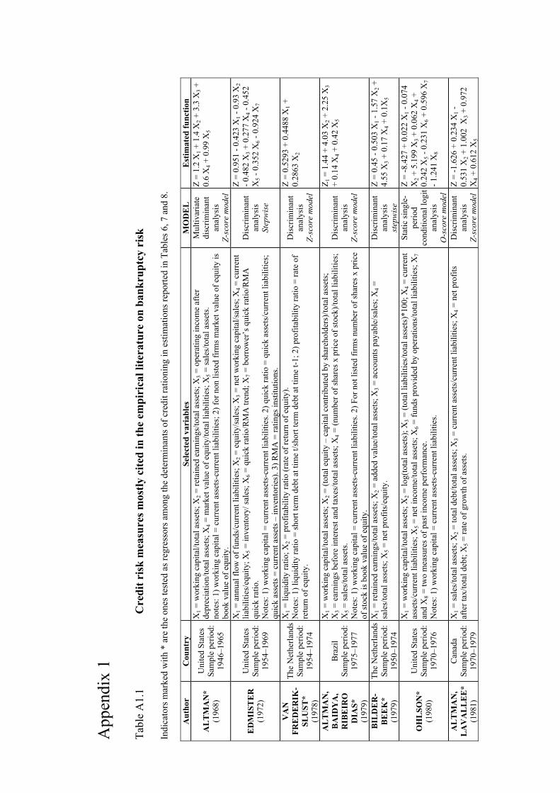
App

endi

x 1

Tabl

e A

1.1

Cre

dit r

isk

mea

sure

s mos

tly c

ited

in th

e em

piri

cal l

itera

ture

on

bank

rupt

cy r

isk

Indi

cato

rs m

arke

d w

ith *

are

the

ones

test

ed a

s reg

ress

ors a

mon

g th

e de

term

inan

ts o

f cre

dit r

atio

ning

in e

stim

atio

ns re

porte

d in

Tab

les 6

, 7 a

nd 8

.

Aut

hor

Cou

ntry

Sele

cted

var

iabl

esM

OD

EL

Est

imat

ed fu

nctio

n

AL

TM

AN

* (1

968)

Uni

ted

Stat

es

Sam

ple

perio

d:

1946

–196

5

X1 =

wor

king

cap

ital/t

otal

ass

ets;

X2 =

reta

ined

ear

ning

s/to

tal a

sset

s; X

3 = o

pera

ting

inco

me

afte

r de

prec

iatio

n/to

tal a

sset

s; X

4 = m

arke

t val

ue o

f equ

ity/to

tal l

iabi

litie

s; X

5 = sa

les/

tota

l ass

ets.

note

s: 1

) wor

king

cap

ital =

cur

rent

ass

ets-

curr

ent l

iabi

litie

s; 2

) for

non

list

ed fi

rms m

arke

t val

ue o

f equ

ity is

bo

ok v

alue

of e

quity

.

Mul

tivar

iate

di

scrim

inan

t an

alys

is

Z-sc

ore

mod

el

Z =

1.2

X1 +

1.4

X2 +

3.3

X3 +

0.

6 X

4 + 0

.99

X5

ED

MIS

TE

R

(197

2)

Uni

ted

Stat

es

Sam

ple

perio

d:

1954

–196

9

X1 =

ann

ual f

low

of f

unds

/cur

rent

liab

ilitie

s; X

2 = e

quity

/sal

es; X

3 = n

et w

orki

ng c

apita

l/sal

es; X

4 = c

urre

nt

liabi

litie

s/eq

uity

; X5 =

inve

ntor

y/ sa

les;

X6 =

qui

ck ra

tio/R

MA

tren

d; X

7 = b

orro

wer

’s q

uick

ratio

/RM

A

quic

k ra

tio.

Not

es: 1

) wor

king

cap

ital =

cur

rent

ass

ets-

curr

ent l

iabi

litie

s. 2)

qui

ck ra

tio =

qui

ck a

sset

s/cu

rren

t lia

bilit

ies;

qu

ick

asse

ts =

cur

rent

ass

ets –

inve

ntor

ies)

. 3) R

MA

= ra

tings

inst

itutio

ns.

Dis

crim

inan

t an

alys

is

Step

wis

e

Z =

0.95

1 - 0

.423

X1 -

0.9

3 X

2 - 0

.482

X3 +

0.2

77 X

4 - 0

.452

X

5 - 0

.352

X6 -

0.9

24 X

7

VA

N

FRE

DE

RIK

-SL

UST

* (1

978)

The

Net

herla

nds

Sam

ple

perio

d:

1954

–197

4

X1 =

liqu

idity

ratio

; X2 =

pro

fitab

ility

ratio

(rat

e of

retu

rn o

f equ

ity).

Not

es: 1

) liq

uidi

ty ra

tio =

shor

t ter

m d

ebt a

t tim

e t/s

hort

term

deb

t at t

ime

t-1; 2

) pro

fitab

ility

ratio

= ra

te o

f re

turn

of e

quity

.

Dis

crim

inan

t an

alys

is

Z-sc

ore

mod

el

Z =

0.52

93 +

0.4

488

X1 +

0.

2863

X2

AL

TM

AN

, B

AID

YA

, R

IBE

IRO

D

IAS*

(1

979)

Bra

zil

Sam

ple

perio

d:

1975

–197

7

X1 =

wor

king

cap

ital/t

otal

ass

ets;

X2 =

(tot

al e

quity

– c

apita

l con

tribu

ted

by sh

areh

olde

rs)/t

otal

ass

ets;

X

3 = e

arni

ngs b

efor

e in

tere

st a

nd ta

xes/

tota

l ass

ets;

X4 =

(num

ber o

f sha

res x

pric

e of

stoc

k)/to

tal l

iabi

litie

s;

X5 =

sale

s/to

tal a

sset

s. N

otes

: 1) w

orki

ng c

apita

l = c

urre

nt a

sset

s-cu

rren

t lia

bilit

ies.

2) F

or n

ot li

sted

firm

s num

ber o

f sha

res x

pric

e of

stoc

k is

boo

k va

lue

of e

quity

.

Dis

crim

inan

t an

alys

is

Z-sc

ore

mod

el

Z 1 =

1.4

4 +

4.03

X2 +

2.2

5 X

3 +

0.14

X4 +

0.4

2 X

5

BIL

DE

R-

BE

EK

* (1

979)

The

Net

herla

nds

Sam

ple

perio

d:

1950

–197

4

X1 =

reta

ined

ear

ning

s/to

tal a

sset

s; X

2 = a

dded

val

ue/to

tal a

sset

s; X

3 = a

ccou

nts p

ayab

le/s

ales

; X4 =

sa

les/

tota

l ass

ets;

X5 =

net

pro

fits/

equi

ty.

Dis

crim

inan

t an

alys

is

step

wis

e

Z =

0.45

- 0.

503

X1 -

1.5

7 X

2 +

4.55

X3 +

0.1

7 X

4 + 0

.1X

5

OH

LSO

N*

(198

0)

Uni

ted

Stat

es

Sam

ple

perio

d:

1970

–197

6

X1 =

wor

king

cap

ital/t

otal

ass

ets;

X2 =

log(

tota

l ass

ets)

; X3 =

(tot

al li

abili

ties/

tota

l ass

ets)

*100

; X4 =

cur

rent

as

sets

/cur

rent

liab

ilitie

s; X

5 = n

et in

com

e/to

tal a

sset

s; X

6 = fu

nds p

rovi

ded

by o

pera

tions

/tota

l lia

bilit

ies;

X7

and

X8 =

two

mea

sure

s of p

ast i

ncom

e pe

rfor

man

ce.

Not

es: 1

) wor

king

cap

ital =

cur

rent

ass

ets-

curr

ent l

iabi

litie

s.

Stat

ic si

ngle

-pe

riod

cond

ition

al lo

git

anal

ysis

O

-sco

re m

odel

Z =

-8.4

27 +

0.0

22 X

1 - 0

.074

X

2 + 5

.199

X3 +

0.0

62 X

4 +

0.24

2 X

5 - 0

.231

X6 +

0.5

96 X

7 - 1

.241

X8

AL

TM

AN

, L

AV

AL

LE

E*

(198

1)

Can

ada

Sam

ple

perio

d:

1970

–197

9

X1 =

sale

s/to

tal a

sset

s; X

2 = to

tal d

ebt/t

otal

ass

ets;

X3 =

cur

rent

ass

ets/

curr

ent l

iabi

litie

s; X

4 = n

et p

rofit

s af

ter t

ax/to

tal d

ebt;

X5 =

rate

of g

row

th o

f ass

ets.

Dis

crim

inan

t an

alys

is

Z-sc

ore

mod

el

Z =

-1.6

26 +

0.2

34 X

1 -

0.53

1 X

2 + 1

.002

X3 +

0.9

72

X4 +

0.6

12 X

5

Aut

hor

Cou

ntry

Sele

cted

var

iabl

esM

OD

EL

Est

imat

ed fu

nctio

n

KO

(1

982)

Japa

n Sa

mpl

e pe

riod:

19

70–1

980

X1 =

EB

IT/s

ales

; X2 =

inve

ntor

y tu

rnov

er 2

yea

rs p

rior/i

nv. t

urno

ver 3

y.p

.; X

3 = st

anda

rd e

rror

of n

et

inco

me

(4 y

ears

); X

4 = w

orki

ng c

apita

l/tot

al d

ebt;

X5 =

mar

ket v

alue

equ

ity/to

tal d

ebt.

Not

es: 1

) wor

king

cap

ital =

cur

rent

ass

ets-

curr

ent l

iabi

litie

s.

Dis

crim

inan

t an

alys

is

Z-sc

ore

mod

el

Z =

0.86

8 X

1 + 0

.198

X2 +

0.

048

X3 +

0.4

36 X

4 +

0.11

5 X

5

ZM

IJE

SKI*

(1

984)

Uni

ted

Stat

es

Sam

ple

perio

d:

1972

–197

8

X1 =

net

inco

me/

tota

l ass

ets;

X2 =

tota

l lia

bilit

ies/

tota

l ass

ets;

X3 =

cur

rent

ass

ets/

curr

ent l

iabi

litie

s. Th

e m

odel

is e

timat

ed u

sing

Unw

eigh

ted

Prob

it (U

p) a

nd W

eigh

ted

Exog

enou

s Sam

ple

Max

imum

Li

kelih

ood

(Wes

ml)

Prob

it

anal

ysis

Up:

Z =

-4.3

36 -

4.51

3 X

1 +

5.67

9 X

2 + 0

.004

X3

Wes

ml:

Z =

-4.8

03 -

3.59

9 X

1 +

5.40

6 X

2 - 0

.100

X3

ZA

VG

RE

N*

(198

5)

Uni

ted

Stat

es

Sam

ple

perio

d:

1972

–197

8

X1 =

tota

l inc

ome/

tota

l ass

ets;

X2 =

sale

s/ne

t pla

nt; X

3 = in

vent

ory/

sale

s; X

4 = d

ebt/t

otal

cap

ital;

X5 =

re

ceiv

able

s; X

6 = q

uick

ass

ets/

curr

ent l

iabi

litie

s/in

vent

ory;

X7 =

cas

h/to

tal a

sset

s. N

otes

: 1) q

uick

ass

ets =

cur

rent

ass

ets –

inve

ntor

ies.

Logi

t m

odel

Z =

-1.5

1150

+ 0

.005

19 X

1 +

0.00

002

X2 +

0.0

6257

X3 +

0.

0182

2 X

4 + 0

.008

29 X

5 -0.

0154

9 X

6 + 0

.422

8 X

7

LO

(1

986)

Uni

ted

Stat

es

Sam

ple

perio

d:

1975

–198

2

X1 =

Log

(tot

al a

sset

s/G

NP

pric

e de

flato

r); X

2 = C

urre

nt d

ebt l

iabi

litie

s/to

tal a

sset

s; X

3 = O

ther

deb

t lia

bilit

ies/

tota

l ass

ets;

X4 =

Cur

rent

ass

ets/

tota

l ass

et; X

5 = N

et in

com

e/to

tal a

sset

s; X

6 = L

o in

dex:

(cas

h +

inta

gibl

es)/c

urre

nt d

ebt l

iabi

litie

s.

Logi

t m

odel

Z =

1.21

40 -

0.04

41 X

1 +

0.10

74 X

2 - 3

.325

8 X

3 - 1

.232

1 X

4 + 1

0.79

71 X

5 - 4

.164

2 X

6

SKO

GSV

IK

(198

8)

Swed

en

Sam

ple

perio

d:

1977

–198

0

X1 =

real

pro

fit b

efor

e ta

xes a

nd in

tere

st/to

tal a

sset

s; X

2 = in

tere

st e

xpen

ses (

nom

inal

)/all

liabi

litie

s and

de

ferr

ed ta

xes;

X3 =

inco

me

taxe

s/re

al b

usin

ess p

rofit

bef

ore

taxe

s; X

4 = in

vent

ory/

reve

nues

; X5 =

ca

sh/c

urre

nt li

abili

ties;

X6 =

ow

ners

’ equ

ity/to

tal a

sset

s; X

7 = re

al g

row

th o

wne

rs’ e

quity

/ow

ners

’ equ

ity; X

8 =

real

gro

wth

unt

axed

rese

rves

/unt

axed

rese

rves

; X9 =

real

real

isab

le g

ain

on in

vent

ory/

inve

ntor

y.

Prob

it

anal

ysis

Z =

-0.9

2 - 2

.78

X1 +

12.

45 X

2 +

1.14

X4 -

0.6

6 X

5 - 3

.13

X6 +

0.

91 X

8 + 2

.49

X9

KE

ASE

Y,

McG

UIN

ESS

(1

990)

Uni

ted

Kin

gdom

Sa

mpl

e pe

riod:

19

76–1

984

X1 =

qui

ck ra

tio; X

2 = 1

/[(to

tal s

ales

– tr

adin

g pr

ofit)

/tota

l cre

dito

rs];

X3 =

turn

over

/net

pla

nt; X

4 = p

re-ta

x pr

ofit

mar

gin.

N

otes

: qui

ck ra

tio =

qui

ck a

sset

s/cu

rren

t lia

bilit

ies.

Logi

t m

odel

step

wis

e

Z =

6.42

02 -

1.55

99 X

1 -

0.30

10 X

2 - 0

.879

9 X

3 - 0

.421

6 X

4 K

EA

SEY

, W

AT

SON

(1

991)

Uni

ted

Kin

gdom

Sa

mpl

e pe

riod:

19

70–1

983

X1 =

(cur

rent

ass

ets –

stoc

k)/c

urre

nt li

abili

ties;

X2 =

tota

l deb

t (in

clus

ive

of o

verd

rafts

)/tot

al a

sset

s; X

3 =

fixed

ass

ets/

tota

l ass

ets;

X4 =

(Pre

Tax

Pro

fit+d

epre

ciat

ion)

/tota

l ass

ets;

X5 =

(Net

pro

fit+i

nter

est)/

Net

W

orth

; X6 =

(Net

pro

fit +

inte

rest

)/tot

al d

ebt.

Logi

t an

alys

is

step

wis

e

Z =

0.60

11+

0.70

48 X

2 -

0.94

93 X

3 - 0

.200

3 X

4 - 0

.124

0 X

5 - 0

.410

4X6

SHU

MW

AY

* (2

001)

Uni

ted

Stat

es

Sam

ple

perio

d:

1962

–199

2

Estim

ates

Altm

an, Z

mije

wsk

i and

a 2

new

form

ulat

ion

usin

g H

azar

d fu

nctio

ns.

Altm

an: X

1 = w

orki

ng c

apita

l/tot

al a

sset

s; X

2 = re

tain

ed e

arni

ngs/

tota

l ass

ets;

X3 =

ope

ratin

g in

com

e af

ter

depr

ecia

tion/

tota

l ass

ets;

X4 =

mar

ket v

alue

of e

quity

/tota

l lia

bilit

ies;

X5 =

sale

s/to

tal a

sset

s; X

6 = ln

(age

) N

otes

: 1) w

orki

ng c

apita

l = c

urre

nt a

sset

s – c

urre

nt li

abili

ties;

2) f

or n

on li

sted

firm

s mar

ket v

alue

of e

quity

is

boo

k va

lue

of e

quity

. Zm

ijew

ski:

X1 =

net

inco

me/

tota

l ass

ets;

X2 =

tota

l lia

bilit

ies/

tota

l ass

ets;

X3 =

cur

rent

ass

ets/

curr

ent

liabi

litie

s; X

4 = ln

(age

) M

arke

t var

iabl

es: X

1 = R

elat

ive

size

; X2 =

pas

t yea

r sto

ck p

erfo

rman

ce; X

3 = id

iosy

ncra

tic st

anda

rd

devi

atio

n of

retu

rns

Mar

ket a

nd a

ccou

ntin

g va

riabl

es: X

1 = n

et in

com

e/to

tal a

sset

s; X

2 = to

tal l

iabi

litie

s/to

tal a

sset

s; X

3 =

Rel

ativ

e si

ze; X

4 = p

ast y

ear s

tock

per

form

ance

; X5 =

idio

sync

ratic

stan

dard

dev

iatio

n of

retu

rns.

Not

es: 1

) wor

king

cap

ital =

cur

rent

ass

ets –

cur

rent

liab

ilitie

s. 2)

rela

tive

size

= lo

g (f

irm’s

mar

ket

capi

talis

atio

n/to

tal m

arke

t cap

italis

atio

n)

Haz

ard

mod

el

Altm

an: Z

= -3

.226

- 0.

732

X1

- 0.8

18 X

2 - 8

.946

X3 -

1.

712

X4 +

0.1

58 X

5 + 0

.15

X6

Zmije

wsk

i: Z

= -7

.811

- 6.

307

X1 +

4.0

68 X

2 - 0

.158

X3

+ 0.

307

X4

Mar

ket v

aria

bles

: Z =

-12.

027

- 0.

503

X1 -

2.07

2 X

2 + 9

.834

X3

Mar

ket a

nd a

ccou

ntin

g va

riabl

es: Z

= -1

3.30

3 -

1.98

2 X

1 + 3

.593

X2 -

0.4

67 X

3 - 1

.809

X4 +

5.7

91 X

5

Aut

hor

Cou

ntry

Sele

cted

var

iabl

esM

OD

EL

Est

imat

ed fu

nctio

n

SAR

ET

TO

* (2

004)

Uni

ted

Stat

es

Sam

ple

perio

d:

1979

–199

6

Estim

ates

Altm

an, O

hlso

n, S

hum

way

, Zm

ijew

ski a

nd 2

new

form

ulat

ions

(Pvt

and

dur

) usi

ng d

urat

ion

anal

ysis

. A

ltman

: X1 =

wor

king

cap

ital/t

otal

ass

ets;

X2 =

reta

ined

ear

ning

s/to

tal a

sset

s; X

3 = o

pera

ting

inco

me

afte

r de

prec

iatio

n/to

tal a

sset

s; X

4 = m

arke

t val

ue o

f equ

ity/to

tal l

iabi

litie

s; X

5 = sa

les/

tota

l ass

ets

Not

es: 1

) wor

king

cap

ital =

cur

rent

ass

ets-

curr

ent l

iabi

litie

s; 2

) for

non

list

ed fi

rms m

arke

t val

ue o

f equ

ity is

bo

ok v

alue

of e

quity

. O

hlso

n: X

1 = w

orki

ng c

apita

l/tot

al a

sset

s; X

2 = lo

g(to

tal a

sset

s); X

3 = (t

otal

liab

ilitie

s/to

tal a

sset

s)*1

00; X

4 =

curr

ent a

sset

s/cu

rren

t lia

bilit

ies;

X5 =

net

inco

me/

tota

l ass

ets;

X6 =

fund

s pro

vide

d by

ope

ratio

ns/to

tal

liabi

litie

s; X

7 and

X8 =

two

mea

sure

s of p

ast i

ncom

e pe

rfor

man

ce

Not

es: 1

) wor

king

cap

ital =

cur

rent

ass

ets-

curr

ent l

iabi

litie

s. Sh

umw

ay: X

1 = to

tal l

iabi

litie

s/to

tal a

sset

s; X

2 = n

et in

com

e/to

tal a

sset

s; X

3 = id

iosy

ncra

tic st

anda

rd

devi

atio

n of

retu

rns;

X4 =

pas

t yea

r sto

ck p

erfo

rman

ce; X

5 = m

easu

re o

f mar

ket c

apita

lisat

ion.

Zm

ijew

ski:

X1 =

tota

l lia

bilit

ies/

tota

l ass

ets;

X2 =

cur

rent

ass

ets/

curr

ent l

iabi

litie

s; X

3 = n

et in

com

e/to

tal

asse

ts.

Mod

el 1

(Pvt

): X

1 = w

orki

ng c

apita

l/tot

al a

sset

s; X

2 = re

tain

ed e

arni

ngs/

tota

l ass

ets;

X3 =

ope

ratin

g in

com

e af

ter d

epre

ciat

ion/

tota

l ass

ets;

X4 =

sale

s/to

tal a

sset

s; X

5 = lo

g(to

tal a

sset

s); X

6 = to

tal l

iabi

litie

s/to

tal a

sset

s;

X7 =

cur

rent

ass

ets/

curr

ent l

iabi

litie

s; X

8 = n

et in

com

e/to

tal a

sset

s; X

9 = fu

nds p

rovi

ded

by o

pera

tions

/tota

l lia

bilit

ies;

X10

and

X11

= tw

o m

easu

res o

f pas

t inc

ome

perf

orm

ance

; X12

= (o

pera

ting

inco

me

– in

tere

st

expe

nses

)/abs

olut

e va

lue

of o

pera

ting

inco

me;

X13

= a

ge.

Mod

el 2

(Dur

) : X

1 = re

tain

ed e

arni

ngs/

tota

l ass

ets;

X2 =

ope

ratin

g in

com

e af

ter d

epre

ciat

ion/

tota

l ass

ets;

X3

= to

tal l

iabi

litie

s/to

tal a

sset

s; X

4 and

X5 =

two

mea

sure

s of p

ast i

ncom

e pe

rfor

man

ce; X

6 = id

iosy

ncra

tic

stan

dard

dev

iatio

n of

retu

rns;

X7 =

pas

t yea

r sto

ck p

erfo

rman

ce; X

8 = lo

g[(r

atio

of m

arke

t cap

italiz

atio

n at

th

e en

d of

the

year

)/ to

tal m

arke

t cap

italiz

atio

n]; X

9 = T

obin

’s Q

; X10

= a

ge.

Dur

atio

n an

alys

is

Altm

an: Z

= 1

.8 X

1 - 0

.081

X2

+ 6.

077

X3 +

0.0

01 X

4 -

0.20

8 X

5 O

hlso

n : Z

= -8

.427

+ 0

.022

X1

- 0.0

74 X

2 +5.

199

X3 +

0.

062

X4 +

0.2

42 X

5 - 0

.231

X6

+ 0.

596

X7 -

1.2

41 X

8 Sh

umw

ay: Z

= -9

.784

+

5.63

9 X

1 - 0

.256

X2 +

2.4

82 X

3 - 1

.004

X4 -

0.0

56 X

5 Zm

ijew

ski:

Z =

-9.4

79 +

6.

384

X1 +

0.0

69 X

2 - 1

.060

X3

Mod

el 1

(Pvt

): Z

= -8

.171

+

0.01

4 X

1 + 0

.388

X2 -

1.9

08 X

3 - 0

.015

X4 -

0.0

32 X

5 +5

.240

X6 +

0.0

57 X

7 +

0.53

4 X

8 + 0

.001

X9 +

0.

478

X10

- 1.

265

X11

- 0.

006

X12

- 0.

024

X13

M

odel

2 (D

ur) :

Z =

-7.2

12 +

0.

277

X1 -

1.7

20 X

2 + 5

.077

X3

+ 0.

331

X4 -

0.9

70 X

5 +

2.63

3 X

6 - 0

.566

X7 +

0.0

39 X

8 - 0

.604

X9 -

0.0

24 X

10

49

Appendix 2

Questionnaire for the VIII Inquiry on Italian manufacturing firms – Year 2001

Section A: General information A.1 Year of birth

A.2 Activity A.2.1 Main Activity

A.2.2 Main products

A.3 Net sales A.3.1 1998 (mill. £) __________________ A.3.2 1999 (mill. £) __________________ A.3.3 2000 (mill. £) __________________ A.4 Share of 2000 net sales from products unchanged in the last three years __________________ A.5 Current legal status � Individually owned � Unlimited liability � Limited liability � Cooperative � Others A.6 Acquisitions and spin-offs A.6.1 Did the firm operate acquisitions, spin-offs or mergers in the period 1998–00? Yes No

A.6.2 Did the firm operate partial acquisitions, spin-offs or mergers in the period 1998–00? Yes No

50

A.7 Ownership structure and control Describe the features of shareholders who own/control the firm in descending order of ownership share N.B. direct control is intended as a determinant influence – exercised through voting power or by appointing members of the board – on medium long term firm goals and on strategies needed to achieve them, on firm’s financial and real development and on investment Type of

owner * (see footnote)

Share of onwership held by the voting owner

Does the owner directly controls the firm ?

Does the owner participate to voting agreements with other shareholders ?

Owner A % Yes No Yes No Owner B % Yes No Yes No Owner C % Yes No Yes No Others % Yes No Yes No Total % Yes No Yes No

* Indicate with 1. Individual of foreign nationality 2. Individual of domestic nationality 3. Private Italian nonfinancial firm 4. State participated Italian nonfinancial firm 5. Private holding 6. State participated holding 7. Banks and other financial institutions

A.8 Groups A.8.1 Does the firm belong to a group ?

Yes No

As a group we indend a set of firms directly or indirectly controlled by the same individual, by the same private or state participated corporation.

A.8.2 The firm is:

Holding Is controlled but controls other firms in the group Subsidiary

A.8.3 How many firms are in the group (including foreign firms)? __________________ A.8.4 When the group has been funded? _______________________________________ A.8.5 Are firms in the group part of the same industry ?

Yes No Partially

51

A.8.6 Do operative relationship exist among firm in the group?

Yes No A.8.7 How many employees are in the group (including foreign subsidiaries)?

A.8.8 Please state the degree of independence of subsidiaries from the holding for each of the following functions A.8.8.1 Administration

controlled by the holding some independence complete independence

A.8.8.2 Finance

controlled by the holding some independence complete independence

A.8.8.3 Marketing

controlled by the holding some independence complete independence

A.8.8.4 R&D

controlled by the holding some independence complete independence

A.9 Consortia A.9.1 Do the firm participate to a consortium?29

Yes No

29 Consortia are contractual agreements ruled by Italian Civil Law among firms which choose to cooperate, to provide common funds and to share information for the development of some common activity (usually internationalisation, R&D and access to credit). They may lead or not to the creation of an independent corporation even though constituents always maintain their independent identity. Consortia differ from cartels and are tolerated by antitrust authorities because their goal is not to restrict competition by altering prices or quantities but just to promote cooperation and economies of scale among associates in order to improve their performance and efficiency.

52

A.9.2 Type of consortium

credit consortium export consortium R&D consortium other consortia

A.9.3 Did the firm used consortium collateral services in the last three years?

Yes No Section B: Labour Force B.1 Employees in 1998–2000 B.1.1 type of workers Owners of the licence for operating the business if managing the business and relatives which work in the firm without fixed wage in case of individual firms. CEO and board executives in case of corporations end of 1998 end of 1999 end of 2000 _.1 Entrepreneurs and supporting relatives _.2 Executives _.3 Intermediate executives _.4 Clerks _.5 Blue collars _.6 Total (_.1+_.2+_.3+_.4+_.5) _.6.4 of which part-time workers _.6.5 of which full time workers _.6.6 of which part time workers (internship)

B.1.2 Employees according to the educational degree Number at 31-12-2000 B.1.2.1 Intermediate school degree B.1.2.2 High school degree B.1.2.3 University degree

B.2.1 Did the firm hired workers in the 1998–2000 period?

Yes No B.2.2 B.2.3 If yes, how many? 1998 9.1.1 Share of graduates 1998 1999 1999 2000 2000

53

B.3 How many employees exited the firm for firing, dismissal, anticipated retirement and other causes in the 1998–2000 period?

1998 1999 2000

B.4 How many employees at point B.1.1 have: 1998 1999 2000 B.4.1 did R&D activity B.4.2 were hired under Employment Training Programs B.4.3 participated to training activity managed by private or state participated training centres

B.5.1 Did the firm used ‘agenzie di lavoro interinale’ in the period 1998–2000? Yes No

B.5.2 How many workers coming from ‘Agenzie di lavoro interinale’ has been employed by the firm in 2000? ________________ B.5.3 On average, for how many months these kind of workers have been employed during 2000?

0–3 months 3–6 months 6–9 months 9–12 months

B.5.4 How many of these workers have been hired by the firm? B.6 On average how many atypical workers collaborate with the firm during one year? Section C: Physical and R&D Investment and technological

innovation activity C.1 Investment C.1.1. Did the firm invest in physical capital in the 1998–2000 period? Yes No

C.1.2 For which amount (millions of liras)? 1998 1999 2000

C.1.3.1 Did the firm invested in hardware, software, networking or telecommunications in the 1998–2000 period? Yes No

54

C.1.3.2 If yes for which total amount in the three years (millions of liras) 1998–2000

C.1.3.3 Indicate the shares of the tree types of investment hardware % software % networking or telecommunications %

C.1.3.4 Indicate the sares per type of application Administrative systems % Production systems % Commercial systems % Internet/Intranet/Extranet % Others %

C.1.4 Which were the goals of physical investment in the 1998–2000 period? (please indicate degree of importance) High Medium Low C.1.4.1 Quality improvement of existing products C.1.4.2 Higher production of existing products C.1.4.3 Production of new products C.1.4.4 Reduced environmental impact C.1.4.5 Reduced raw material utilisation C.1.4.6 Reduced manpower utilisation C.1.4.7 Other goals

C.1.5 How was physical investment financed in the 1998–2000 period? C.1.5.1 Equity capital (%) %C.1.5.2 Internal finance (%) %C.1.5.3 Short term loans (%) %C.1.5.4 Medium-long term loans at market rates (%) %C.1.5.5 Medium-long term soft loans (%) %C.1.5.6 State grants (%) %C.1.5.7 Tax allowances (%) %C.1.5.8 Leasing (%) %C.1.5.9 Intergroup lending (%) %C.1.5.10 Industrial lenders (%) %C.1.5.11 Others (%) %

55

C.2 Technological innovation research and development C.2.1. Did the firm realise in the 1998–2000 period product innovations process innovations organisational innovations related to product innovations Neither of the above

C.2.2.1 Did the firm incurred in R&D expenditures? Yes No

C.2.2.2 For which amount? 1998 1999 2000

C.2.2.3 Which was the contribution of Internal research labs %External research labs %

C.2.2.3.3 And, among external labs: Universities %External research centres %Other firms %Other %

C.2.2.4 How much of R&D expenditure was devoted to C.2.2.4.1 Improvement of existing processes %C.2.2.4.2 Improvement of existing products %C.2.2.4.3 Introduction of new processes %C.2.2.4.4 Introduction of new products %C.2.2.4.5 Others %

C.2.2.5 How was the R&D expenditure financed (% on total amount)? C.2.2.5.1 Equity capital %C.2.2.5.2 Internal finance %C.2.2.5.3 Medium-long term loans at market rates %C.2.2.5.4 Medium-long term soft loans %C.2.2.5.5 State or EEC grants %C.2.2.5.6 Tax allowances %C.2.2.5.7 Others %

56

Section D: Internationalisation D.1 Export D.1 Did the firm export part or all its production in 2000? Yes No

D.1.2 Export geographic breakdown

Geographical areas % EU Russia and Central-Eastern Europe Other European countries Africa United States and Canada Central and South America Middle East and other Asian countries China Australia and Oceania Other D.2 The firm in the 1998–2000 period D.2.1 Purchased patents or licences from abroad?

Yes, from EU countries

Yes, from other industrialised countries

Yes, from other non-industrialised countries

No

D.2.2 Sold patents or licences from abroad?

Yes, from EU countries

Yes, from other industrialised countries

Yes, from other non-industrialised countries

No

D.2.3 Stipulated productive agreements with foreign firms?

Yes, from EU countries

Yes, from other industrialised countries

Yes, from other non-industrialised countries

No

D.2.4 Stipulated trade agreements with foreign firms?

Yes, from EU countries

Yes, from other industrialised countries

Yes, from other non-industrialised countries

No

57

D.2.5 Did foreign direct investment to produce abroad?

Yes, from EU countries

Yes, from other industrialised countries

Yes, from other non-industrialised countries

No

D.2.5.2 If yes to question D.2.5, indicate year and amount in million liras EU

1998 1999 2000

Non EU industrialised countries

1998 1999 2000

Non EU non-industrialised countries

1998 1999 2000

D.2.6.1 Did the firm created sale structures abroad in the 1998–2000 period?

Yes, from EU countries

Yes, from other industrialised countries

Yes, from other non-industrialised countries

No

Of which: Directly managed local fixed structures

EU countries Other industrialised

countries

Other non industrialised

countries Fixed structures managed by local traders

EU countries Other industrialised

countries

Other non industrialised

countries Fixed structures managed by participated companies

EU countries Other industrialised

countries

Other non industrialised

countries Other types of promotional activities

EU countries Other industrialised

countries

Other non industrialised

countries D.2.7.1 Was the firm consulted by Italian individuals or institutions?

Yes, from EU countries

Yes, from other industrialised countries

Yes, from other non-industrialised countries

No

58

EU countries Other industrialised

countries

Other non industrialised

countries Institute for Foreign Trade Embassies Chambers of Commerce Banks Regional institutions Others

Section E: The market E.1 2000 Net sales breakdown according to customers and trading channel characteristics E.1.1 Domestic distributive channels % E.1.2 Foreign distributive channels % E.1.3 Specialised intermediaries (wholesalers, buyers) % E.1.4 Intermediaries specialised in goods for firms % E.1.5 Direct sale to firms % E.1.6 Direct sale to customers % E.1.7 Franchising % E.1.8 Other %

E.2 2000 Net sales breakdown according to …. E.2.1 Subcontracting % E.2.2 Direct sale %

For subcontracting we mean an industrial relationship by which a firm entrusts another with the execution of a step of its own productive process or of an activity linked to the productive process itself, or of the provision of intermediate inputs or components which will be integrated in a more complex product E.3 Breakdown of subcontracted net sales in 2000 (item E.2.1) Firms belonging to the same group in The same province % The rest of Italy % Abroad %

Other firms in The same province % The rest of Italy % Abroad %

59

E.4. Localisation of the main firm’s competitors Same province Same region Other Italian regions EU countries Other industrialised countries LDC

E.5 Size of competitors Large Medium Small

E.6. Did the firm received ISO9000 (quality) certification? Yes No E.7 Does the firm measure customer’s satisfaction? Yes No Section F: Finance F.1 Relationship with banks F.1.1 Indicate the number of banks with which the firm

had a commercial relationship at the end of 2000

F.1.2 Share of firm bank debt held by the main lender at the end of 2000

%

F.1.3 Is the main bank lender located in the same province of the firm? Yes No

F.1.4 Since how many years is it the main lender? ____________________________ F.1.5 In the year 2000 had the company desired more credit at the market interest rate? Yes No

F.1.6 Had the company been willing to pay a higher interest rate in order to obtain more credit? Yes No

60

F.1.7 Did the company demanded in the year 2000 more credit without obtaining it? Yes No

F.2 Innovating financial instruments and equity capital F.2.1 Has the firm made use of innovative financial instruments from 1998 on? Yes No

Which ones?

F.2.2 Will the firm make use of innovative financial instruments in the next 3 years? Yes No

F.2.3 Has any financial operator underwritten venture capital in the firm from 1998 to today? Yes No

F.2.4 Is the firm ready to yield venture capital minority shares to banks, merchant banks, financial holding companies, closed-end funds or other financial operators in the years to come? Yes No

F.2.5 Has the firm yielded venture capital shares to non-financial private operators? Yes No

F.2.6 Is the firm listed at the stock exchange? Yes No

F.2.7 If no, is it willing to go public in the next three years? Yes No

F.3 Subsidies F.3.1.1.1 Has the firm applied for any type of financial subsidies in 1998–2000 period? Yes No

61

F.3.1.1.2 If yes, check below the type of subsidy required Law 1329/65 (Sabatini)

Law 317/91

Other laws supporting Small and Medium Sized Firms

Laws supporting applied research and technological innovation: Law 46/82

Fund for technological innovation (Art. 14–19 Law 46/82)

Laws to stimulate investment in depressed areas: Law 488/92

Law ‘Visco’ to stimulate investments

DIT Dual Income Tax

Industry Guarantees

Tax allowances for firms investing in depressed areas

Low interest credit for export programs (loans and insurance): Law 227/77

External market trade penetration programs: Law 394/81

Other laws (Specify number and objective of each law)

Regional laws (Specify number and objective of each law)

Other laws (Specify number and objective of each law)

F.4 Financial Management F.4 1.1 The firm’s financial management is carried out by:

own personnel

external intermediaries

F.4.1.2 External financial intermediaries are in charge of: Cash position management in Liras or foreign currency

Administrative services (collection-payments)

Guaranties – bank guaranties – banker’s acceptances

Export finance operations

62

Derivatives (forwards, futures, swaps) Project financing

Other operations

F.4.2.1 Has the firm planned a strategy to develop its own financial management? Yes No

F.4.2.2 If yes, which are the main means? Own personnel

Intermediaries

-National

-Foreign

-External consultants

F.4.3 Breakdown of the firm's financial investment? Participation in Italian firms %

Participation in foreign firms %

Italian short term securities %

Foreign short term securities %

Italian long and mid term securities % Foreign long and mid term securities %

Other Italian derivative instruments %

Other foreign derivative instruments %

BANK OF FINLAND RESEARCH DISCUSSION PAPERS ISSN 0785-3572, print; ISSN 1456-6184, online 1/2008 Peik Granlund Regulatory choices in global financial markets – restoring

the role of aggregate utility in the shaping of market supervision. 2008. 36 p. ISBN 978-952-462-416-9, print; ISBN 978-952-462-417-6, online.

2/2008 Ari Hyytinen – Tuomas Takalo Consumer awareness and the use of

payment media: evidence from Young Finnish consumers. 2008. 34 p. ISBN 978-952-462-418-3, print; ISBN 978-952-462-419-0, online.

3/2008 Patrick M Crowley One money, several cycles? Evaluation of European

business cycles using model-based cluster analysis. 2008. 47 p. ISBN 978-952-462-420-6, print; ISBN 978-952-462-421-3, online.

4/2008 József Molnár Market power and merger simulation in retail banking.

2008. 26 p. ISBN 978-952-462-422-0, print; ISBN 978-952-462-423-7, online. 5/2008 Heli Huhtala Along but beyond mean-variance: Utility maximization in a

semimartingale model. 2008. 29 p. ISBN 978-952-462-426-8, print; ISBN 978-952-462-427-5, online.

6/2008 Mikael Juselius Cointegration implications of linear rational expectation

models. 2008. 25 p. ISBN 978-952-462-428-2, print; ISBN 978-952-462-429-9, online.

7/2008 Tuomas Takalo – Tanja Tanayama – Otto Toivanen Evaluating innovation

policy: a structural treatment effect model of R&D subsidies. 2008. 59 p. ISBN 978-952-462-430-5, print; ISBN 978-952-462-431-2, online.

8/2008 Essi Eerola – Niku Määttänen On the importance of borrowing constraints

for house price dynamics. 2008. 40 p. ISBN 978-952-462-432-9, print; ISBN 978-952-462-433-6, online.

9/2008 Marko Melolinna Using financial markets information to identify oil supply

shocks in a restricted VAR. 2008. 35 p. ISBN 978-952-462-434-3, print; ISBN 978-952-462-435-0, online.

10/2008 Bill B Francis – Iftekhar Hasan – James R Lothian – Xian Sun The signalling

hypothesis revisited: Evidence from foreign IPOs. 2008. 41 p. ISBN 978-952-462-436-7, print; ISBN 978-952-462-437-4, online.

11/2008 Kari Takala – Matti Viren Efficiency and costs of payments: some new evidence from Finland. 2008. 50 p. ISBN 978-952-462-438-1, print; ISBN 978-952-462-439-8, online.

12/2008 Jukka Topi Bank runs, liquidity and credit risk. 2008. 31 p. ISBN 978-952-462-440-4, print; ISBN 978-952-462-441-1, online. 13/2008 Juha Kilponen – Matti Viren Why do growth rates differ? Evidence from

cross-country data on private sector production. 2008. 29 p. ISBN 978-952-462-442-8, print; ISBN 978-952-462-443-5, online. 14/2008 Bill B Francis – Iftekhar Hasan – Delroy M Hunter Does hedging tell the full

story? Reconciling differences in US aggregate and industry-level exchange rate risk premia. 2008. 58 p. ISBN 978-952-462-444-2, print;

ISBN 978-952-462-445-9, online. 15/2008 Leonardo Becchetti – Annalisa Castelli – Iftekhar Hasan Investment-cash

flow sensitivities, credit rationing and financing constraints. 2008. 64 p. ISBN 978-952-462-446-6, print; ISBN 978-952-462-447-3, online.

Suomen PankkiBank of FinlandP.O.Box 160FI-00101 HELSINKIFinland