47
Investment Course III – November 2007 Topic One: Expected Returns & Measuring the Risk Premium
| Date post: | 28-Dec-2015 |
| Category: |
Documents |
| Upload: | tobias-parsons |
| View: | 214 times |
| Download: | 0 times |

Investment Course III – November 2007
Topic One:
Expected Returns & Measuring the Risk Premium

1 - 2
Some Important Concepts Involving Expected Investment Returns
1. Investors perform two functions for capital markets:- Commit Financial Capital- Assume Risk
so,
E(R) = (Risk-Free Rate) + (Risk Premium)
2. The expected return (i.e., E(R)) of an investment has a number of alternative names: e.g., discount rate, cost of capital, cost of equity, yield to maturity. It can also be expressed as:
k = (Nominal RF) + (Risk Premium)= [(Real RF) + E(Inflation)] + (Risk Premium)
where:
Risk Premium = f (business risk, liquidity risk, political risk, financial risk)
3. Investors can be compensated in two ways:- Period Cash Flows- Capital Gain
so,
E(R) = E(Cash Flow) + E(Capital Gain)

1 - 3
Rt = (1 + Rft) (1+ RPt) – 1
or
Rt = (1 + Inft) (1 + RRft) (1 + RPt) – 1
where Rt = return on asset class for year t,
Inft = inflation rate
Rft = risk free rate
RRft = real risk free rate
RPt = risk premium
RPt =
where RRt = real asset class return
Measuring Expected Returns: Overview
Risk Premium
1 + Rft
1 + Rt - 1 =1 + RRft
1 + RRt - 1

1 - 4
Developing Expected Return Assumptions With the Risk Premium Approach
March, 2005 18
T bills
Real Interest
Rate
Inflation
Term Premium
Credit Risk
Premium
T notes
CorpBonds
USEquities
Equity Risk
Premium
3.00%
1.00%
1.40%
1.25%
1.5% to 2.0%
4.00%
5.40%6.65%
8.15%to
8.65%T bills
Real Interest
Rate
Real Interest
Rate
InflationInflation
Term Premium
Term Premium
Credit Risk
Premium
Credit Risk
Premium
T notes
CorpBonds
USEquities
Equity Risk
Premium
Equity Risk
Premium
3.00%
1.00%
1.40%
1.25%
1.5% to 2.0%
4.00%
5.40%6.65%
8.15%to
8.65%

1 - 5
Methods for Estimating the Equity Risk Premium
1. Historical Evidence
2. Fundamental Estimates
3. Economic Estimates
4. Surveys

1 - 6
Estimating the Equity Risk Premium
1. Historical Evidence: Representative Work
– Ibbotson Associates – US Markets (2006)
– Fidelity Investments - Global Markets (2004)
– Jorion and Goetzmann (Journal of Finance, 1999)
– Siegel (Financial Analysts Journal, 1992)
– Dimson, Marsh and Staunton (Business Strategy Review, 2000)

1 - 7
Ibbotson Associates U.S. Return & Risk Data: 1926 - 2006
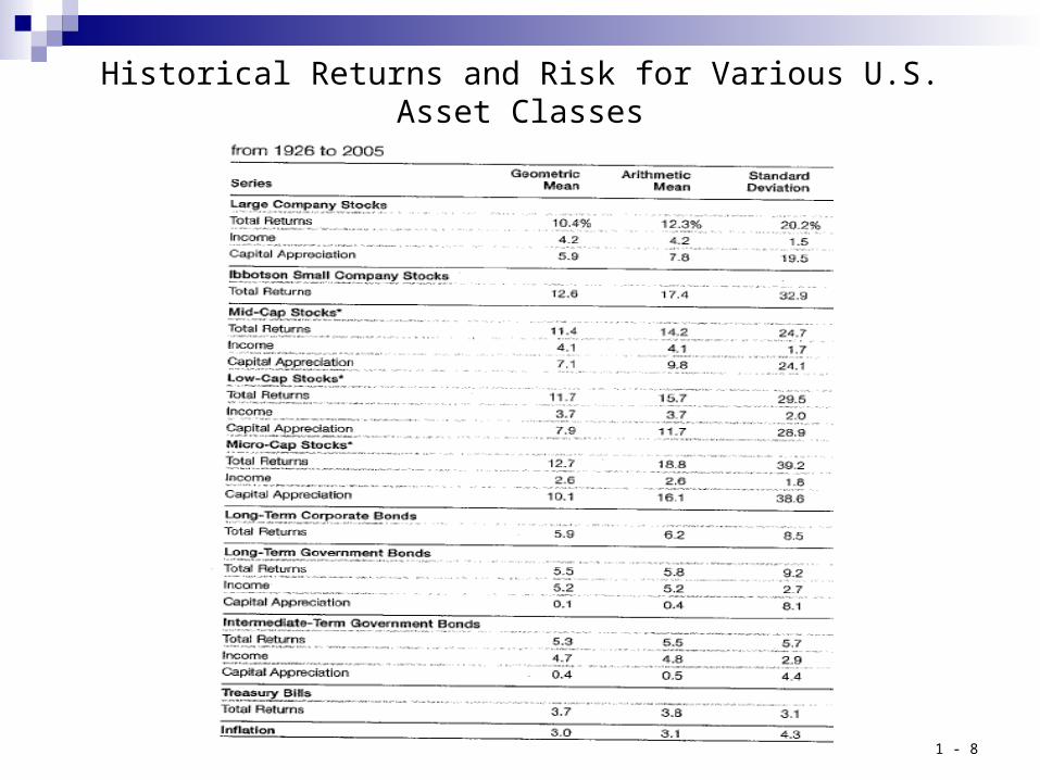
1 - 8
Historical Returns and Risk for Various U.S. Asset Classes
1 - 9
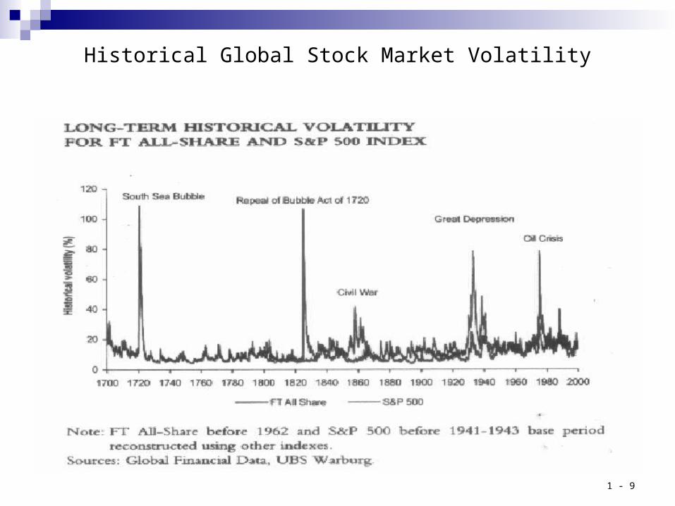
Historical Global Stock Market Volatility

1 - 10
U.S. Equity Return Histogram
199919981996
2005 2006 19891992 2004 19831987 1993 19791984 1988 1976 20031978 1986 1967 1997
1994 1970 1982 1963 19951990 1960 1972 1961 1991
2001 1981 1956 1971 1955 19852000 1977 1953 1968 1951 19801973 1966 1948 1965 1950 19751969 1946 1947 1964 1949 1945
2002 1962 1941 1939 1959 1944 19361974 1957 1940 1934 1952 1943 1928 1958 1954
1931 1937 1930 1929 1932 1926 1942 1938 1927 1935 1933-50 -40 -30 -20 -10 0 10 20 30 40 50 60
Annual Stock Market Return (%)

1 - 11
International Equity Histogram
2006*20041999
1997 19982002 1996 2005 1988 20032000 1994 1995 1987 1993
2001 1992 1984 1991 1983 19781990 1973 1982 1979 1989 1980 19751974 1970 1981 1976 1977 1971 1972 1985 1986
-30 -20 -10 0 10 20 30 40 50 60 70
Annual Non-U.S. Stock Return (%)
1 - 12
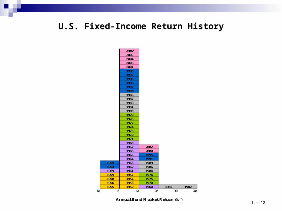
U.S. Fixed-Income Return History
2006*200520042003200119981997199619931992199019881987198319811980197919781977197419731972197119681967 20021966 20001965 19951964 1991
1999 1963 19891994 1962 19861969 1961 19841959 1957 19761958 1954 19751956 1953 19701955 1952 1960 1985 1982
-10 0 10 20 30 40
Annual Bond Market Return (%)

1 - 13
More on Historical Asset Class Returns: U.S. Experience
Stocks:
Bonds:
T-Bills:
Inflation:
1926-2006: Avg. Return 12.34% 6.22% 3.77% 3.11% Std. Deviation 20.08% 8.46% 3.10% 4.26% 1982-2006: Avg. Return 14.45 11.81 5.36 3.09 Std. Deviation 15.54 10.90 2.52 1.16 1997-2006: Avg. Return 10.02 8.08 3.61 2.38 Std. Deviation 19.14 6.61
1.79 0.75
2002-2006: Avg. Return 7.63 8.20 2.32 2.58 Std. Deviation 18.79 4.80 1.56 0.72 Source: Ibbotson Associates

1 - 14
Historical Risk Premia vs. T-bills: U.S. Experience
Stocks: Bonds:
Stock - Bond
Difference:
1926-2006: 8.57% 2.45% 6.12%
1982-2006: 9.09 6.45 2.64
1997-2006: 6.41 4.47 1.94
2002-2006: 5.31 5.88 -0.57

1 - 15
Data for Historical Global Analysis
Series Starting Dates
Stocks Bonds Stocks Bonds
Argentina Jan-1988 May-1991 Italy Jan-1925 Jan-1862Australia Nov-1882 Jan-1859 Japan Jan-1921 Dec-1870Austria Jan-1970 Aug-1945 Mexico Jan-1970 Jan-1995Belgium Jan-1951 Jul-1832 Netherlands Jan-1951 Nov-1915Canada Jan-1934 Sep-1855 New Zealand Aug-1986 Mar-1925Chile Feb-1927 Jan-1993 Norway Jan-1970 Dec-1876Denmark Jan-1970 Jul-1821 Portugal Jan-1988 Jan-1976Finland Jan-1962 Jan-1960 South Africa Mar-1960 Dec-1860France Mar-1895 Mar-1800 Spain May-1940 Dec-1940Germany Jan-1870 Jan-1924 Sweden Jan-1919 Jan-1922Greece Jan-1977 n/a Switzerland Mar-1966 Mar-1915Ireland Jan-1988 Jun-1928 UK Oct-1694 Aug-1700Israel Jan-1993 Nov-1993 USA Mar-1871 Mar-1800
Source: Global Financial Data

1 - 16
Historical Real Returns, 1954-2003: The Global Experience
Historical Real Returns, 1954-2003
0%
1%
2%
3%
4%
5%
6%
7%
8%
9%
Ann
ually
Com
poun
ded
Rea
l Ret
urn,
%
Equities
Bonds
Chile: Returns 1/54 – 6/03Chile*: Returns 1/54 – 12/71; 1/76 – 6/03Source: Global Financial Data
1 - 17
Global Historical Volatility Measures, 1954-2003
Historical Risk, 1954-2003
0%
5%
10%
15%
20%
25%
30%
35%
40%
Ann
ually
Com
pou
nded
Rea
l Ret
urn,
%
Equities
Bonds
1 - 18
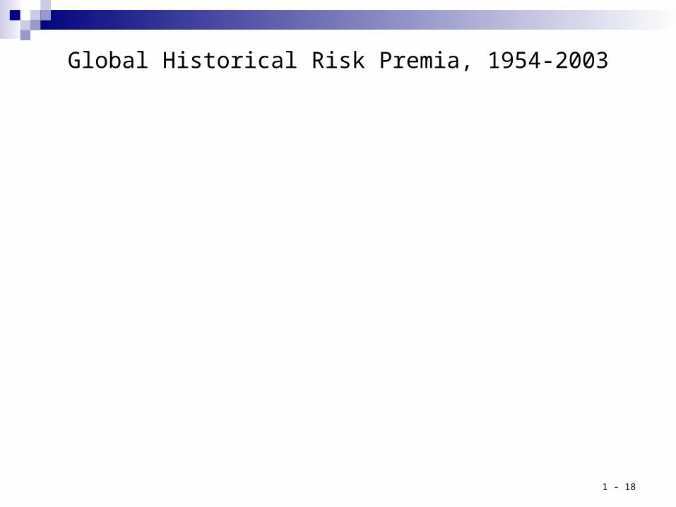
Global Historical Risk Premia, 1954-2003
Risk Premia of Stocks and Bonds to Cash, 1954-2003
-2%
0%
2%
4%
6%
8%
10%
12%
14%
16%
18%
Ann
ually
Com
poun
ded
Rea
l Ret
urn,
%
Equities-CashBonds-Cash

1 - 19
Estimating the Equity Risk Premium (cont.)
2. Fundamental Estimates: Representative Work
– Fama and French (University of Chicago, 2000)
– Ibbotson and Chen (Yale University, 2001)
– Claus and Thomas (Journal of Finance, 2001)
– Arnott and Bernstein (Financial Analysts Journal, 2002)

1 - 20
Fundamental Risk Premium Estimates: An Overview
One potential problem with using historical averages to estimate future expected returns is that there is no way to control for the possibility that the past data sample you selected produced averages that are “abnormal” (i.e., too high or too low) in some way.
Another problem we have seen is that historical average returns tend to be fairly unstable (i.e., they are extremely sensitive to the time period chosen in the analysis).
Fundamental risk premium estimates attempt to objectively forecast the expected returns that would normally occur, given the fundamental relationships that tend to exist in the capital markets. In other words, fundamental forecasts attempt to link return expectations to the economic conditions likely to pertain in the market during the forecast interval.

1 - 21
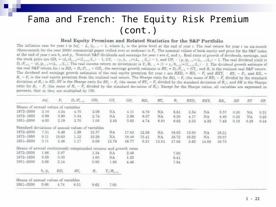
Fama and French: The Equity Risk Premium
Main Idea: Use dividend and earnings growth rates to measure the expected rate of capital gains for equity investments. This process creates two ways of then estimating real (i.e., inflation-adjusted) expected equity returns:a. E(R) = E(Div Yld) + E(Real Growth Rate of Dividends) = RDb. E(R) = E(Div Yld) + E(Real Growth Rate of Earnings) = RY
Notice that the intuition behind this approach is simply that it is possible to compensated investors in two ways: cash flow and capital gain. This is sometimes referred to as a demand-side approach to estimating the risk premium.
Real Equity Risk Premium can then be estimated by subtracting short-term commercial paper yields from RD and RY, which leaves RXD and RXY, respectively.
Main Result: Using data from the period 1951 to 2000 for the US market (i.e., S&P 500), they find that:- RXD = 2.55%- RXY = 4.32%
Notice that both of these fundamental risk premium estimates are well below the average historical risk premium during the period (i.e., 7.43%), leading the authors that future expected returns to equity investments are unlikely to match the high levels of the recent past.
1 - 22
Fama and French: The Equity Risk Premium (cont.)

1 - 23
Claus and Thomas: Equity Risk Premia in US and International Markets
Main Idea: Based on the notion that the fundamental value of an equity investment can be described by its book value plus the present value of future abnormal earnings.
This valuation can be estimated by a modified version of the multi-stage growth model:
where the discount rate k (= rf + rp) is the equity expected return.
Main Results: Using observed market data (e.g., p, bv) and analyst forecasts (e.g., g) for the other inputs over 1985-1998, the authors calculate the values of the equity risk premium (rp) that solve the model:
- US: 3.40%- Japan: 0.21%- UK: 2.81%- France: 2.60%- Canada: 2.23%
1t
t00 rp) rf (1
)gae(1 bv p

1 - 24
Claus and Thomas: Estimates of Equity Risk Premia for US Markets
1 - 25
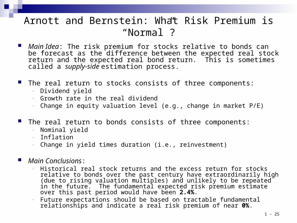
Arnott and Bernstein: What Risk Premium is “Normal”?
Main Idea: The risk premium for stocks relative to bonds can be forecast as the difference between the expected real stock return and the expected real bond return. This is sometimes called a supply-side estimation process.
The real return to stocks consists of three components:- Dividend yield- Growth rate in the real dividend- Change in equity valuation level (e.g., change in market P/E)
The real return to bonds consists of three components:- Nominal yield- Inflation- Change in yield times duration (i.e., reinvestment)
Main Conclusions: - Historical real stock returns and the excess return for stocks relative to bonds
over the past century have extraordinarily high (due to rising valuation multiples) and unlikely to be repeated in the future. The fundamental expected risk premium estimate over this past period would have been 2.4%.
- Future expectations should be based on tractable fundamental relationships and indicate a real risk premium of near 0%.

1 - 26
Arnott and Bernstein: What Risk Premium is “Normal”? (cont.)

1 - 27
Estimating the Equity Risk Premium (cont.)
3. Economic Estimates: Representative Work
– Black and Litterman (1992, 2007)
– Asset Class-Specific Risk Premia
– Ennis Knupp Associates (2007)
1 - 28
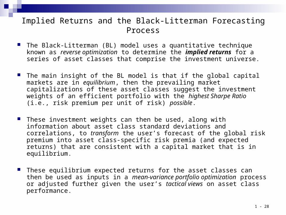
Implied Returns and the Black-Litterman Forecasting Process
The Black-Litterman (BL) model uses a quantitative technique known as reverse optimization to determine the implied returns for a series of asset classes that comprise the investment universe.
The main insight of the BL model is that if the global capital markets are in equilibrium, then the prevailing market capitalizations of these asset classes suggest the investment weights of an efficient portfolio with the highest Sharpe Ratio (i.e., risk premium per unit of risk) possible.
These investment weights can then be used, along with information about asset class standard deviations and correlations, to transform the user’s forecast of the global risk premium into asset class-specific risk premia (and expected returns) that are consistent with a capital market that is in equilibrium.
These equilibrium expected returns for the asset classes can then be used as inputs in a mean-variance portfolio optimization process or adjusted further given the user’s tactical views on asset class performance.
1 - 29
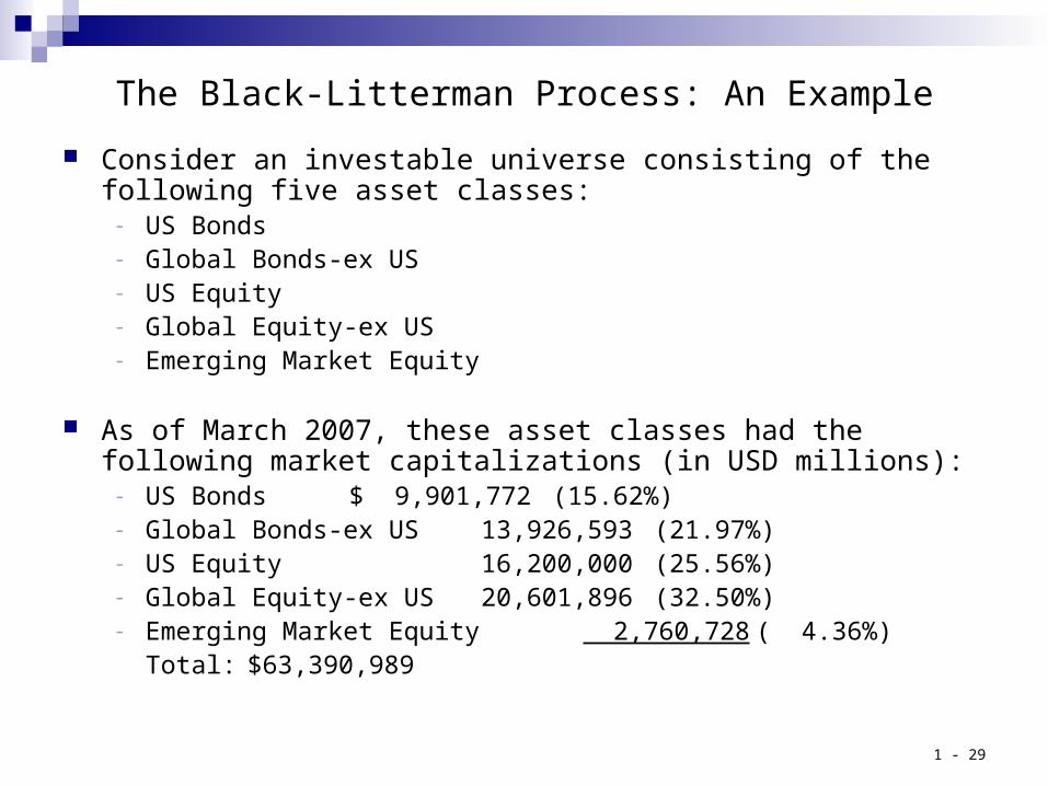
The Black-Litterman Process: An Example
Consider an investable universe consisting of the following five asset classes:
- US Bonds- Global Bonds-ex US- US Equity- Global Equity-ex US- Emerging Market Equity
As of March 2007, these asset classes had the following market capitalizations (in USD millions):
- US Bonds $ 9,901,772 (15.62%)
- Global Bonds-ex US 13,926,593 (21.97%)- US Equity 16,200,000 (25.56%)- Global Equity-ex US 20,601,896 (32.50%)- Emerging Market Equity 2,760,728 ( 4.36%)
Total: $63,390,989

1 - 30
Black-Litterman Example (cont.)
Consider also the following historical return standard deviations (March 2002 – March 2007):
usb = 3.84% gb = 8.27% uss = 12.30%
gs = 13.24% ems = 17.46%
The historical correlation matrix, measured using all available pairwise historical return data:
usb,gb = 0.55 gb,gs = 0.13
usb,uss = -0.28 gb,ems = 0.05
usb,gs = -0.15 uss,gs = 0.86
usb,ems = -0.10 uss,ems = 0.77
gb,uss = -0.13 gs,ems = 0.89

1 - 31
Black-Litterman Example (cont.)
The remaining inputs that the user must specify are: (i) the global risk premium of the investment universe, and (ii) the risk-free rate. Using current market data we have:
- Global Risk Premium: 4.14% (10-yr Global Balanced)
- Risk-Free Rate: 4.63% (10-yr US Treasury)
The heart of the BL process is to then calculate the implied excess return for each asset class, using the following (stylized) formula:
[Risk Aversion Parameter] x [Covariance Matrix] x [Market Cap Weight Vector]

1 - 32
Black-Litterman Example (cont.)
The risk aversion parameter is the rate at which more return is required as compensation for more risk. It is calculated as:
RAP = [Global Risk Premium] / [Market Portfolio Variance]
It can be shown in this example that the market portfolio variance is (8.09%)2 = 0.654%, so that:
RAP = (0.0414)/(0.00654) = 6.33
The covariance between two asset classes (Y and Z) is given by the formula:
Cov(Y,Z) = y,z x y x z
For instance, the covariance between US Equity and Global Equity-ex US is: (0.86) x (12.30%) x (13.24%) = 0.014
1 - 33
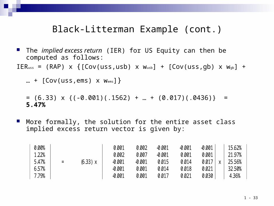
Black-Litterman Example (cont.)
The implied excess return (IER) for US Equity can then be computed as follows:
IERuss = (RAP) x {[Cov(uss,usb) x wusb] + [Cov(uss,gb) x wgb] +
… + [Cov(uss,ems) x wems]}
= (6.33) x {(-0.001)(.1562) + … + (0.017)(.0436)} = 5.47%
More formally, the solution for the entire asset class implied excess return vector is given by:
0.00% 0.001 0.002 -0.001 -0.001 -0.001 15.62% 1.22% 0.002 0.007 -0.001 0.001 0.001 21.97% 5.47% = (6.33) x -0.001 -0.001 0.015 0.014 0.017 x 25.56% 6.57% -0.001 0.001 0.014 0.018 0.021 32.50% 7.79% -0.001 0.001 0.017 0.021 0.030 4.36%

1 - 34
Black-Litterman Example (cont.)
The total expected return for US Equity is then simply the IER plus the risk-free rate:
4.63% + 5.47% = 10.10%
The excess and total expected returns for the other asset classes in this example are:
Excess Total
- US Bonds: 0.00% 4.63%- Global Bonds: 1.22% 5.85%- Global Equity: 6.57% 11.20%- Emerging Equity: 7.79% 12.42%

1 - 35
Black-Litterman Example: Excel Spreadsheet

1 - 36
Black-Litterman Example: Proprietary Software (Zephyr Associates)
Asset Allocation Analysis Zephyr AllocationADVISOR: LBJ Asset Management Partners
Analysis InputsCase: Allocation Case
Analysis InputsForecast Date Constraint
Return Risk Start End Min Max
AssetsUS Bonds 4.6% 3.8% Mar 2002 Mar 2007 0% 100%
Global Bonds xUSD 5.9% 8.3% Mar 2002 Mar 2007 0% 100%US Equity 10.1% 12.3% Mar 2002 Mar 2007 0% 100%
Global Equity xUS 11.2% 13.2% Mar 2002 Mar 2007 0% 100%Emerging Equity 12.4% 17.5% Mar 2002 Mar 2007 0% 100%
BenchmarkS&P 500 10.0% 12.3% Mar 2002 Mar 2007
Projection InputsTarget Return: 10.0%Time Horizon: 10 Years
Initial Value: $1,000,000
Correlations1 2 3 4 5
1. US Bonds 1.002. Global Bonds xUSD 0.55 1.003. US Equity -0.28 -0.13 1.004. Global Equity xUS -0.15 0.13 0.86 1.005. Emerging Equity -0.10 0.05 0.77 0.89 1.00
Black-Litterman Model InputsPalette Risk Premium 4.14%
Risk-free Rate 4.63%
Market Cap(millions) Date Weight
US Bonds $9,901,772 Mar 2007 15.62%Global Bonds xUSD $13,926,593 Mar 2007 21.97%
US Equity $16,200,000 Mar 2007 25.56%Global Equity xUS $20,601,896 Mar 2007 32.50%
Emerging Equity $2,760,728 Mar 2007 4.36%

1 - 37
Ennis Knupp Associates (EKA) – January 2007
EKA uses a similar process to the BL methodology in that they develop asset class expected return forecasts that are grounded in the notion that the global capital markets are in equilibrium.
Specifically, EKA estimates asset class expected returns to be consistent with a global Capital Asset Pricing Model (CAPM). Two expected return “anchors” are used as a starting point:
- US Equity = 8.6%: Total return is divided into three components: dividend yield (1.7%), nominal growth rate of corporate earnings (6.9%), and change in valuation levels (0%)
- US Bonds = 5.6%: Based on two components: current yield and simulated future changes in yields (based on forecasts of expected inflation, inflation risk premium, and real yields)

1 - 38
EKA Fundamental Expected Return Estimates (cont.)
Other asset class expected returns are then estimated relative to these anchors using the global CAPM. Specifically, expected returns on the various asset classes are proportional to their systematic risk levels relative to the global market portfolio, shown at the right.
For example, the ratio of the US Bonds beta (0.40) to the US Equity beta (1.71) is 0.24. This implies that the ratio of US Bond risk premium to US Equity risk premium should also be 24%.
Therefore:
(5.6 – RF)/(8.6 – RF) = 0.24
which results in an implied risk-free rate of 4.7%. The risk premium of each asset class is then calculated so that it is directly proportional to its systematic risk, given these two anchors

1 - 39
EKA Fundamental Expected Return Estimates (cont.)
1 - 40
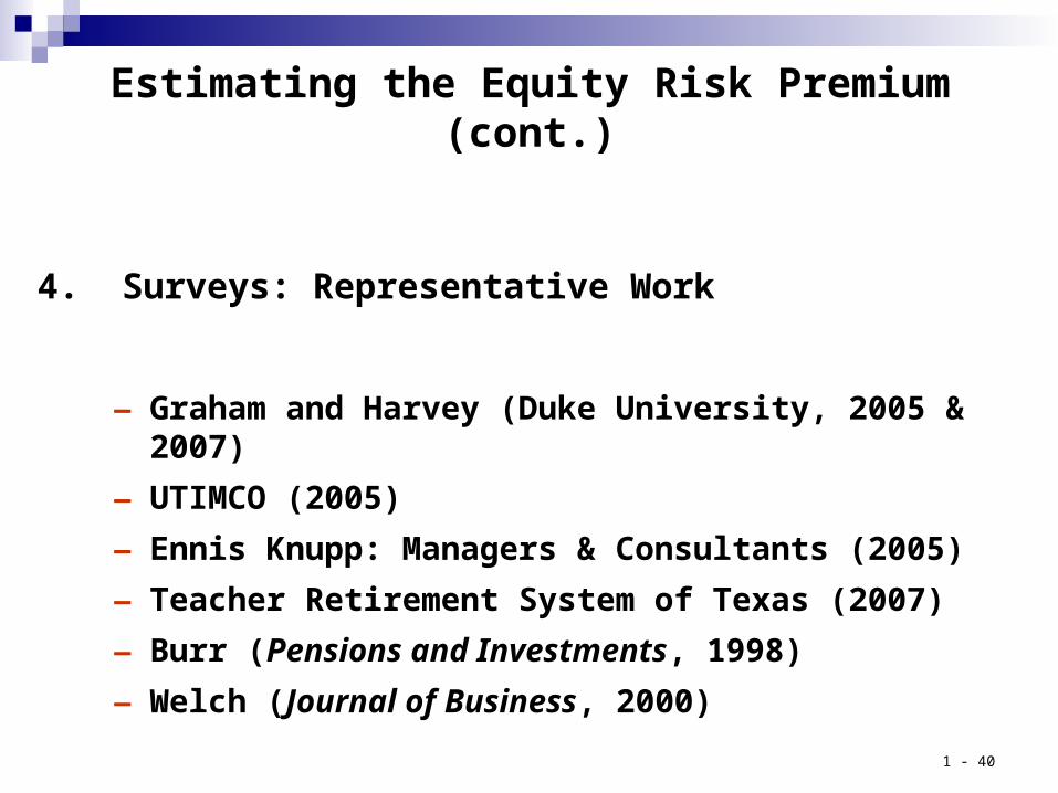
Estimating the Equity Risk Premium (cont.)
4. Surveys: Representative Work
– Graham and Harvey (Duke University, 2005 & 2007)
– UTIMCO (2005)
– Ennis Knupp: Managers & Consultants (2005)
– Teacher Retirement System of Texas (2007)
– Burr (Pensions and Investments, 1998)
– Welch (Journal of Business, 2000)

1 - 41
Campbell-Harvey Survey of Corporate CFOs – June 2005

1 - 42
Campbell-Harvey Survey of Corporate CFOs – January 2007

1 - 43
Survey of Asset Class Return & Risk Expectations:UTIMCO Staff & External Expert Opinions – March 2005
March, 2005 20
Asset CategoryCambridge Associates
Goldman Sachs
Wilshire Associates
BridgeWater BGIEnnisKnupp
10 yearsCitigroup
Consultant Average
HistoricalUTIMCO
2003UTIMCO
2005
US Equity Nominal Returns 10.00% 8.00% 9.20% 7.90% 8.06% 8.80% 10.00% 8.85% 11.53% 8.50% 8.50% Real Returns 7.00% 5.80% 6.95% 5.00% 6.06% 6.30% 7.50% 6.37% 6.86% 5.50% 5.50% Std Deviation 17.00% 17.30% 17.00% 15.50% 15.50% 17.00% 15.79% 16.44% 15.82% 17.00% 17.00%
Global Equity Nominal Returns 10.00% 7.70% 9.75% 7.60% 8.06% NA 10.00% 8.85% 11.86% 8.50% 8.50% Real Returns 7.00% 5.50% 7.50% 4.70% 6.06% NA 7.50% 6.38% 7.19% 5.50% 5.50% Std Deviation 20.00% 17.40% 20.00% 14.50% 16.25% 19.00% 15.23% 17.48% 16.77% 19.00% 19.00%
Emerging Markets Equity Nominal Returns 13.00% 8.30% 11.40% 9.30% 9.14% NA 10.90% 10.34% 15.04% 11.00% 10.50% Real Returns 10.00% 6.10% 9.15% 6.40% 7.14% NA 8.40% 7.86% 10.36% 8.00% 7.50% Std Deviation 28.00% 23.60% 27.00% 21.00% 25.00% NA 24.22% 24.80% 23.25% 26.00% 26.00%
Absolute Return Hedge Funds Nominal Returns 7.00% 8.40% 6.82% NA NA NA 5.40% 6.91% 10.79% 7.00% 7.00% Real Returns 4.00% 6.20% 4.57% NA NA NA 2.90% 4.42% 6.12% 4.00% 4.00% Std Deviation 9.00% 4.90% 8.00% NA NA NA 4.06% 6.49% 6.15% 7.50% 7.50%
Directional Hedge Funds Nominal Returns 9.00% 8.40% 6.82% NA NA NA 9.60% 8.46% 10.48% 8.00% 8.00% Real Returns 6.00% 6.20% 4.57% NA NA NA 7.10% 5.97% 5.81% 5.00% 5.00% Std Deviation 13.00% 4.90% 8.00% NA NA NA 7.56% 8.37% 8.16% 11.00% 10.00%
Venture Capital Nominal Returns 15.00% NA 15.25% 10.30% NA NA 16.40% 14.24% 15.16% 14.00% 14.00% Real Returns 12.00% NA 12.99% 7.40% NA NA 13.90% 11.57% 10.49% 11.00% 11.00% Std Deviation 28.00% NA 30.00% 25.00% NA NA 43.50% 31.63% 18.78% 30.00% 30.00%
1 - 44
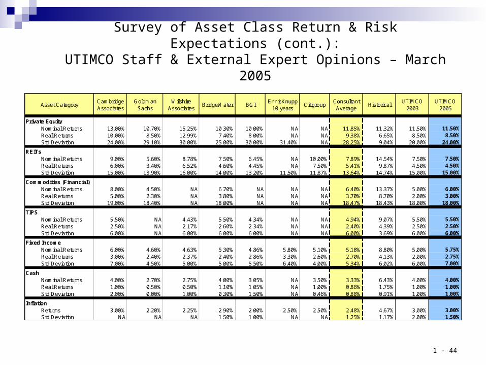
Survey of Asset Class Return & Risk Expectations (cont.):UTIMCO Staff & External Expert Opinions – March 2005
March, 2005 21
Asset CategoryCambridge Associates
Goldman Sachs
Wilshire Associates
BridgeWater BGIEnnisKnupp
10 yearsCitigroup
Consultant Average
HistoricalUTIMCO
2003UTIMCO
2005
Private Equity Nominal Returns 13.00% 10.70% 15.25% 10.30% 10.00% NA NA 11.85% 11.32% 11.50% 11.50% Real Returns 10.00% 8.50% 12.99% 7.40% 8.00% NA NA 9.38% 6.65% 8.50% 8.50% Std Deviation 24.00% 29.10% 30.00% 25.00% 30.00% 31.40% NA 28.25% 9.04% 20.00% 24.00%
REITs Nominal Returns 9.00% 5.60% 8.78% 7.50% 6.45% NA 10.00% 7.89% 14.54% 7.50% 7.50% Real Returns 6.00% 3.40% 6.52% 4.60% 4.45% NA 7.50% 5.41% 9.87% 4.50% 4.50% Std Deviation 15.00% 13.90% 16.00% 14.00% 13.20% 11.50% 11.87% 13.64% 14.74% 15.00% 15.00%
Commodities (Financial) Nominal Returns 8.00% 4.50% NA 6.70% NA NA NA 6.40% 13.37% 5.00% 6.00% Real Returns 5.00% 2.30% NA 3.80% NA NA NA 3.70% 8.70% 2.00% 3.00% Std Deviation 19.00% 18.40% NA 18.00% NA NA NA 18.47% 18.43% 18.00% 18.00%
TIPS Nominal Returns 5.50% NA 4.43% 5.50% 4.34% NA NA 4.94% 9.07% 5.50% 5.50% Real Returns 2.50% NA 2.17% 2.60% 2.34% NA NA 2.40% 4.39% 2.50% 2.50% Std Deviation 6.00% NA 6.00% 6.00% 6.00% NA NA 6.00% 3.69% 6.00% 6.00%
Fixed Income Nominal Returns 6.00% 4.60% 4.63% 5.30% 4.86% 5.80% 5.10% 5.18% 8.80% 5.00% 5.75% Real Returns 3.00% 2.40% 2.37% 2.40% 2.86% 3.30% 2.60% 2.70% 4.13% 2.00% 2.75% Std Deviation 7.00% 4.50% 5.00% 5.00% 5.50% 6.40% 4.00% 5.34% 6.02% 6.00% 7.00%
Cash Nominal Returns 4.00% 2.70% 2.75% 4.00% 3.05% NA 3.50% 3.33% 6.43% 4.00% 4.00% Real Returns 1.00% 0.50% 0.50% 1.10% 1.05% NA 1.00% 0.86% 1.75% 1.00% 1.00% Std Deviation 2.00% 0.00% 1.00% 0.30% 1.50% NA 0.46% 0.88% 0.91% 1.00% 1.00%
Inflation Returns 3.00% 2.20% 2.25% 2.90% 2.00% 2.50% 2.50% 2.48% 4.67% 3.00% 3.00% Std Deviation NA NA NA 1.50% 1.00% NA NA 1.25% 1.17% 2.00% 1.50%
1 - 45
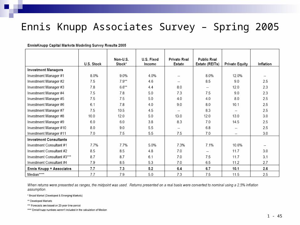
Ennis Knupp Associates Survey – Spring 2005
1 - 46
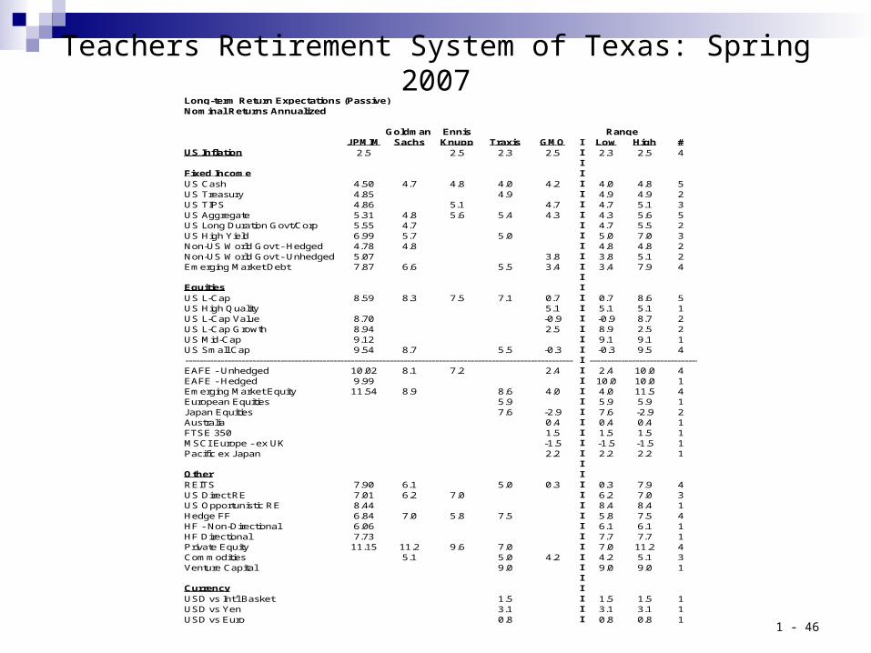
Teachers Retirement System of Texas: Spring 2007Long-term Return Expectations (Passive)Nominal Returns Annualized
Goldman Ennis RangeJPMIM Sachs Knupp Traxis GMO I Low High #
US Inflation 2.5 2.5 2.3 2.5 I 2.3 2.5 4I
Fixed Income IUS Cash 4.50 4.7 4.8 4.0 4.2 I 4.0 4.8 5US Treasury 4.85 4.9 I 4.9 4.9 2US TIPS 4.86 5.1 4.7 I 4.7 5.1 3US Aggregate 5.31 4.8 5.6 5.4 4.3 I 4.3 5.6 5US Long Duration Govt/Corp 5.55 4.7 I 4.7 5.5 2US High Yield 6.99 5.7 5.0 I 5.0 7.0 3Non-US World Govt - Hedged 4.78 4.8 I 4.8 4.8 2Non-US World Govt - Unhedged 5.07 3.8 I 3.8 5.1 2Emerging Market Debt 7.87 6.6 5.5 3.4 I 3.4 7.9 4
IEquities IUS L-Cap 8.59 8.3 7.5 7.1 0.7 I 0.7 8.6 5US High Quality 5.1 I 5.1 5.1 1US L-Cap Value 8.70 -0.9 I -0.9 8.7 2US L-Cap Growth 8.94 2.5 I 8.9 2.5 2US Mid-Cap 9.12 I 9.1 9.1 1US Small Cap 9.54 8.7 5.5 -0.3 I -0.3 9.5 4-------------------------------------------------------------------------------------------------------------------I --------------------------------EAFE - Unhedged 10.02 8.1 7.2 2.4 I 2.4 10.0 4EAFE - Hedged 9.99 I 10.0 10.0 1Emerging Market Equity 11.54 8.9 8.6 4.0 I 4.0 11.5 4European Equities 5.9 I 5.9 5.9 1Japan Equities 7.6 -2.9 I 7.6 -2.9 2Australia 0.4 I 0.4 0.4 1FTSE 350 1.5 I 1.5 1.5 1MSCI Europe - ex UK -1.5 I -1.5 -1.5 1Pacific ex Japan 2.2 I 2.2 2.2 1
IOther IREITS 7.90 6.1 5.0 0.3 I 0.3 7.9 4US Direct RE 7.01 6.2 7.0 I 6.2 7.0 3US Opportunistic RE 8.44 I 8.4 8.4 1Hedge FF 6.84 7.0 5.8 7.5 I 5.8 7.5 4HF - Non-Directional 6.06 I 6.1 6.1 1HF Directional 7.73 I 7.7 7.7 1Private Equity 11.15 11.2 9.6 7.0 I 7.0 11.2 4Commodities 5.1 5.0 4.2 I 4.2 5.1 3Venture Capital 9.0 I 9.0 9.0 1
ICurrency IUSD vs Int'l Basket 1.5 I 1.5 1.5 1USD vs Yen 3.1 I 3.1 3.1 1USD vs Euro 0.8 I 0.8 0.8 1
1 - 47
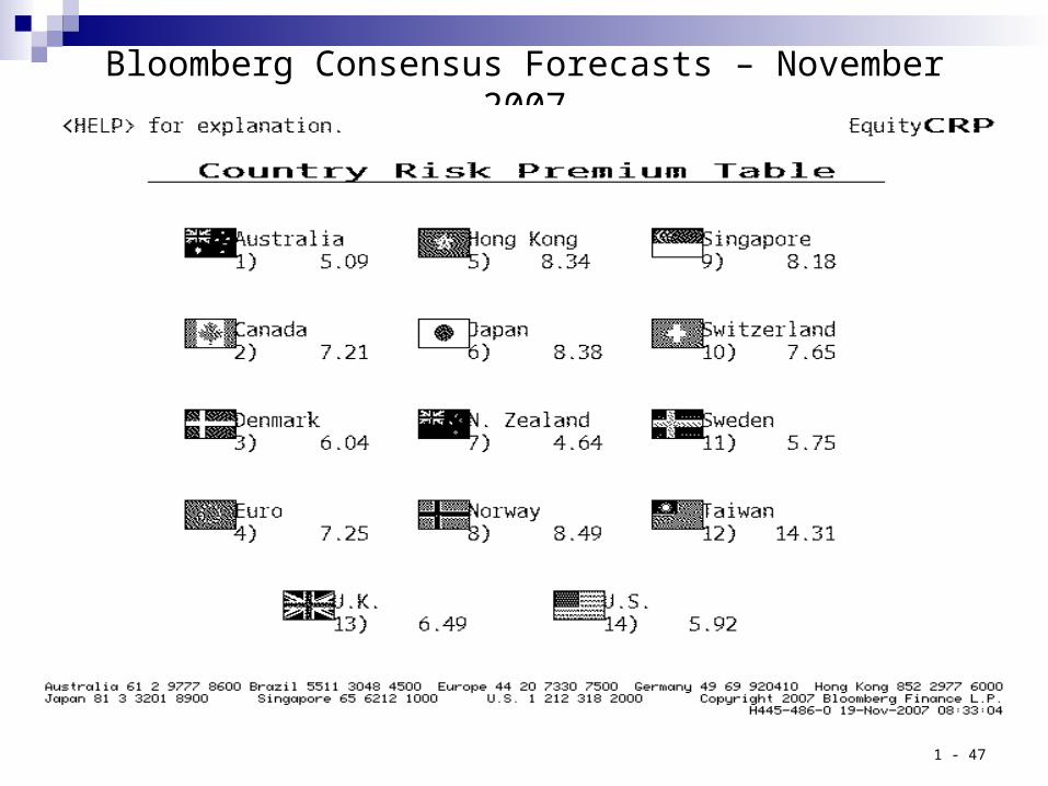
Bloomberg Consensus Forecasts – November 2007


