Investment Timing, Agency and Information∗

Steven R. Grenadier† Neng Wang‡

March 2004

Abstract

This paper provides a model of investment timing by managers in a decentralizedfirm in the presence of agency conflicts and information asymmetries. When investmentdecisions are delegated to managers, contracts must be designed to provide incentives formanagers to both extend effort and truthfully reveal private information. Using a realoptions approach, we show that an underlying option to invest can be decomposed intotwo components: a manager’s option and an owner’s option. The implied investmentbehavior differs significantly from that of the first-best no-agency solution. In particular,there will be greater inertia in investment, as the model predicts that the manager willhave a more valuable option to wait than the owner.

∗We thank Tony Bernardo, Peter DeMarzo, Harrison Hong, John Long, Erwan Morellec, Mike Raith, DavidScharfstein, Bill Schwert, Cliff Smith, Jeff Zwiebel, seminar participants at 2004 AFA (San Diego), Columbiaand Rochester, and especially Mike Barclay, Rene Stulz (the editor) and an anonymous referee for helpfulcomments.

†Graduate School of Business, Stanford University and NBER. Email: sgren@stanford.edu.‡Corresponding author. William E. Simon School of Business Administration, University of Rochester.

Email: wang@simon.rochester.edu.

1 Introduction

One of the most important topics in corporate finance is the formulation of the optimal

investment strategies of firms. There are two components of the investment decision: how

much to invest and when to invest. The first is the capital allocation decision and the

second is the investment timing decision. The standard textbook prescription for the capital

allocation decision is that firms should only invest in projects if their net present values

(NPV) are positive. Similarly, a standard framework for the investment timing decision is

the real options approach. The real options approach posits that the opportunity to invest in

a project is analogous to an American call option on the investment project, and the timing

of investment is economically equivalent to the optimal exercise decision for an option. The

real options approach is well summarized in Dixit and Pindyck (1994) and Trigeorgis (1996).1

However, both the simple NPV rule and the standard real options approach fail to ac-

count for the presence of agency conflicts and information asymmetries. In most modern

corporations, shareholders delegate the investment decision to managers, taking advantage

of managers’ special skills and expertise. In such decentralized settings, there are likely to

be both information asymmetries (e.g., managers are better informed than owners about

projected cash flows) and agency issues (e.g., unobserved managerial effort, perquisite con-

sumption, empire building). A number of papers in the corporate finance literature provide

models of capital budgeting under asymmetric information and agency.2 The focus of this

literature is on the first element of the investment decision: the amount of capital allocated

to managers for investment. Thus, this literature provides predictions on whether firms over-

or under-invest relative to the first-best no-agency benchmark. The focus of this paper is

on the second element of the investment decision: the timing of investment. We extend the

real options framework to account for the issues of information and agency in a decentralized

firm. Analogous to the notions of over- or under-investment, our paper provides results on

hurried or delayed investment.1The application of the real options approach to investment is quite broad. Brennan and Schwartz (1985)

use an option pricing approach to analyze investment in natural resources. McDonald and Siegel (1986)provided the standard continuous-time framework for analysis of a firm’s investment in a single project. Majdand Pindyck (1987) enrich the analysis with a time-to-build feature. Dixit (1989) uses the real option approachto examine entry and exit from a productive activity. Triantis and Hodder (1990) analyze manufacturingflexibility as an option. Titman (1985) and Williams (1991) use the real options approach to analyze realestate development.

2See Stein (2001) for a useful summary.

1

In the standard real options paradigm, there are no agency conflicts as it is assumed that

the option’s owner makes the exercise decision.3 However, in this paper, an owner delegates

the option exercise decision to a manager. Thus, the timing of investment is determined by

the manager. The owner’s problem is to design an optimal contract under both hidden action

and hidden information. The true quality of the underlying project can be high or low. The

hidden action problem is that the manager can influence the likelihood that the quality of

the project is high. An optimal contract will have the property that the manager will be

induced to provide costly (but unverifiable) effort. The hidden information problem is that

the underlying project’s future value contains a component that is only privately observed

by the manager. Absent any mechanism that induces the manager to reveal his private

information voluntarily, the manager may have an incentive to lie about the true quality of

the project and divert value for his private interests. For example, the manager could divert

privately observed project value by consuming excessive perquisites, building empires, or by

working less hard. An optimal contract will induce the manager to deliver to the owner the

true value of the privately observed component of project value, and thus no actual value

diversion will take place in equilibrium.

Importantly, we show that the underlying option can be decomposed into two components:

a “manager’s option” and an “owner’s option.” The manager’s option has a payout upon

exercise that is a function of the contingent compensation contract. Based on this contractual

payout, the manager determines the exercise time. The owner’s option has a payout, received

at the manager’s chosen exercise time, equal to the payoff from the underlying option minus

the manager’s compensation. The model provides the solution for the optimal contract that

comes as close as possible to the first-best no-agency solution.

The model implies investment behavior that differs substantially from that of the standard

real options approach with no agency problems. In general, managers will display greater

inertia in their investment behavior, in that they will invest later than implied by the first-

best solution. In essence, this is a result of the manager (even in an optimal contract) not

having a full ownership stake in the option payoff. This less than full ownership interest

implies that the manager has a more valuable “option to wait” than the owner.3While our paper focuses on the agency issues that arise from the divergence of interests between owners

and shareholders, similar issues exist between stockholders and bondholders. Mello and Parsons (1992), Mauerand Triantis (1994), Leland (1998), Mauer and Ott (2000), and Morellec (2001, 2003) examine the impact ofagency conflicts on firm value using the real options approach.

2

An important aspect of the model is the interaction of hidden action and hidden infor-

mation. We find that the nature of the optimal contract depends explicitly on the relative

importance of these two forces. While we focus on the economically most interesting case

in which both forces play a role in the optimal contract, it is instructive to consider two

extremes. If the cost benefit ratio of inducing effort (a measure of the strength of the hid-

den effort component) is very low, then the hidden action component disappears from the

optimal contract terms. Thus, if the nature of the underlying option is such that inducing

effort is sufficiently inexpensive, then we are left with a simple problem of hidden informa-

tion and the contract will simply reward the manager with information rents. This is similar

to the setting of Maeland (2002), which considers a real options problem with only hidden

information about the exercise cost.4 Conversely, as the cost benefit ratio of inducing effort

becomes very high, then the hidden action component dominates the optimal contract. The

cost of inducing effort is so high as to no longer necessitate the payment of information rents.

When the cost benefit ratio of inducing effort is in the intermediate range, both forces are

in effect, and the optimal contract must induce both effort and truthful revelation of private

information. Interestingly, the interplay between hidden information and hidden action may

actually reduce the inefficiency in investment timing, compared with the setting in which

hidden information is the only friction. This is because the manager’s additional option to

exert effort makes his incentives more closely aligned with those of the owner.

We further generalize the model to allow managers to display greater impatience than

owners. There are several potential justifications for such an assumption. First, there are

various models of managerial myopia that attempt to explain managers’ preferences for choos-

ing projects with quicker pay-backs, even in the face of eschewing more valuable long-term

opportunities.5 Such models are based on information asymmetries and agency problems.

Second, in our “investment timing” setting, greater impatience can represent the manager’s

preference for empire building or greater perquisite consumption and reputation that comes

from running a larger company sooner rather than later. Third, managers may simply have

shorter horizons (due to job loss, alternative job offers, death, etc.). Phrased in real options4Bjerksund and Stensland (2000) provide a similar model to Maeland (2002), where a principal delegates

an investment decision to an agent who holds private information about the investment’s cost. Brennan(1990) considers a setting in which managers attempt to signal the true quality of “latent” assets to investorsthrough converting them into observable assets (e.g., exercising real options).

5See Narayanan (1985), Stein (1989) and Bebchuk and Stole (1993).

3

terms, managerial impatience decreases the value of the manager’s option to wait. While the

base case model predicts that investment will never occur sooner than the first-best case, in

this generalized setting investment can occur either earlier or later than the first-best case.

The setting of our paper is most similar to that of Bernardo et al. (2001). In a de-

centralized firm under asymmetric information and moral hazard, they examine the capital

allocation decision, while we examine the investment timing decision. In their model, the

firm’s headquarters delegates the investment decision to a manager, who possesses private

information about project quality. The manager can improve project quality through the

exertion of effort, which is costly to the manager but unverifiable by headquarters. These

two assumptions mirror our framework. In addition, managers have preferences for “empire

building” in that they derive utility from overseeing large investment projects. This assump-

tion is addressed in the generalized version of our model that appears in Section 5. Absent

any explicit incentive mechanism, managers will always claim that all projects are of high

quality and worthy of funding, and then provide the minimal amount of effort. As in our

paper, they use an optimal contracting approach to jointly derive the optimal investment

and compensation policies. An incentive contract is derived that induces truth-telling and

minimizes agency costs. In equilibrium, they find that there will be under-investment in all

states of the world. Our model provides an intertemporal analogy to their equilibrium: in

our base case model, we find that in equilibrium there will be delayed investment due to the

information asymmetries and agency costs.6

While our paper derives an optimal contract that best aligns the incentives of owners

and managers, other papers in the corporate finance literature analyze the capital budgeting

problem under information asymmetry and agency using other control mechanisms. Harris

et al. (1982) consider the case of capital allocation in a decentralized firm with multiple

division managers. Managers have private information about project values. In addition,

managers have private interests in overstating investment requirements, and then diverting6In a different setting, Holmstrom and Ricart i Costa (1986) provide a model that combines an optimal

wage contract with capital rationing. In their model, the manager and the market learn about managerialtalent over time by observing investment outcomes. A conflict of interest arises because the manager wantsto choose investment to maximize the value of his human capital while the shareholders want to maximizefirm value. The optimal wage contract has the option feature that insures the manager against the possibilitythat an investment reveals his ability to be of low quality, but allows the manager to captures the gains if heis revealed to be of high quality. This option feature of the wage contract encourages the manager to take onexcessive risks. Rationing capital mitigates the manager’s incentive to overinvest. As a result, in equilibriumboth under- and over-investment are possible.

4

the excess cash flows in order to minimize effort or to consume greater perquisites. They

focus on the role of transfer prices in allocating capital. Firms offer managers a menu of

allocation/transfer price combinations. In equilibrium, truth-telling is achieved, and there can

be both under- and over-investment.7 Harris and Raviv (1996) use a very similar framework,

but focus on a random auditing technology. By combining probabilistic auditing with a

capital restriction, headquarters is able to learn the true project quality from the manager.

In equilibrium there will be both regions of under- and over-investment. Stulz (1990) considers

a decentralized investment framework in which the manager has private information about

investment quality and a preference for empire building. Absent any controls, the manager

would always overstate the investment opportunities and invest all available cash. The owners

of the firm use debt as a mechanism to align the interests of managers and shareholders.

By increasing the required debt payment, managers have less free cash flow to spend on

investment projects. The optimal level of debt is chosen to trade off the benefits of preventing

managers from investing in negative NPV projects when investment opportunities are poor

with the costs of rationing managers away from taking positive NPV projects when investment

opportunities are good. Again, in equilibrium there will be both under- and over-investment.

The remainder of the paper is organized as follows. Section 2 describes the setup of the

model. Section 3 simplifies the optimization program and solves for the optimal contracts.

In Section 4, we analyze the implications of the model in terms of the stock price’s reaction

to investment, equilibrium investment lags, and the erosion of the option value due to the

agency problem. Section 5 generalizes the model to allow for managers to display greater

impatience than owners. Section 6 concludes. Appendices contain the solution details of the

optimal contracts.

2 Model

In this section, we begin with a description of the model. We then, as a useful benchmark,

provide the solution to the first-best no-agency investment problem. Finally, we present the

full principal-agent optimization problem faced by the owner.7Antle and Eppen (1985) provide a model that is very similar to that of Harris et al (1982).

5

2.1 Setup

The principal owns an option to invest in a single project. We assume that the principal

(owner) delegates the exercise decision to an agent (manager). Once investment takes place,

the project generates two sources of value. One portion is observable and contractible to

both the owner and the manager, while the other portion is privately observed only by the

manager. Let P (t) represent the observable component of the project’s value, and θ the value

of the privately observed component. Thus, the total value of the project is P (t) + θ.8

In a standard call option setting, exercise yields the difference between the observable

value P (t) of the underlying asset and the exercise price, K. Thus, the payoff from exercise

is typically P (t) −K. However, in the present model, the payoff from exercise also includes

a privately observed random variable, θ, whose realization directly impacts the option payoff.

Thus, in this model the net payoff from exercise is P (t) + θ − K. Note that the problem

could be equivalently formulated as one in which the total value of the project is P (t) and

the effective cost of exercising the option is K − θ.

Let the value P (t) of the observable component of the underlying project evolve as a

geometric Brownian motion:

dP (t) = αP (t) dt + σP (t) dz(t), (1)

where α is the instantaneous conditional expected percentage change in P (t) per unit time,

σ is the instantaneous conditional standard deviation per unit time, and dz is the increment

of a standard Wiener process. Let P0 equal the value of the project at time zero, in that

P0 = P (0). Both the owner and the manager are risk neutral, with the risk-free rate of

interest denoted by r.9 For convergence, we assume that r > α.

The assumption that a portion of project value is only observed by the manager and not

verifiable by the owner is quite common in the capital budgeting literature. This information

asymmetry invites a host of agency issues. Harris et al. (1982) posit that managers have8For ease of presentation, we model the process P (t) for the present value of observable cash flows. We

could back up a step, and begin with an underlying process for observable cash flows. However, if observablecash flows follow a geometric Brownian motion, then the present value of expected future observable cashflows will also follow a geometric Brownian motion as above. Similarly, rather than modeling θ as the presentvalue of unobservable cash flows, we could begin with an underlying process for the unobservable cash flowsthemselves.

9We rule out the time-zero selling-the-firm contract between the owner and the manager. This may bejustified, for example, if the manager is liquidity constrained and cannot obtain financing.

6

incentives to understate project payoffs and to divert the free cash flow to themselves. In

their model, such value diversion takes the form of managers reducing their level of effort.

Stulz (1990), Harris and Raviv (1996) and Bernardo et al. (2001) model managers as having

preferences for perquisite consumption or empire building. In these models, managers have

incentives to divert free cash flows to inefficient investments or to excessive perquisites. In all

of these models, mechanisms are used by firms (i.e., incentive contracts, auditing, required

debt payments) to mitigate such value diversion.

The private component of value, θ, may take on two possible values: θ1 or θ2, with

θ1 > θ2.10 We denote ∆θ = θ1 − θ2 > 0. One may interpret a draw of θ1 as a “higher

quality” project and a draw of θ2 as a “lower quality” project. Although the owner cannot

observe the true value of θ, the owner does observe the amount handed over by the manager

upon exercise. While in theory the manager could attempt to hand over θ2 when the true

value is θ1, it will be seen in equilibrium that the amount transferred to the owner at exercise

will always be the true value.11

The effort of the manager plays an important role in determining the likelihood of obtain-

ing a higher quality project. The manager may affect the likelihood of drawing θ1 by exerting

a one-time effort, at time zero. If the manager exerts no effort,12 the probability of drawing

a higher quality project θ1 equals qL. However, if the manager exerts effort, he incurs a cost

ξ > 0 at time zero, but increases the likelihood of drawing a higher quality project θ1 from

qL to qH . Immediately after his exerting effort at time zero, the manager observes the private

component of project quality. In order to ensure a positive “net” exercise price, we restrict

θ1 < K.

Although the owner cannot contract on the private component of value, θ, he can contract

on the observable component of value, P (t). Contingent on the level of P (t) at exercise,

the manager is paid a wage.13 The manager has limited liability and is always free to walk10In Section 3.3 we generalize the model to allow θ to have continuous distributions.11Off the equilibrium path, the manager could attempt to hand over θ2 when the true value is θ1. As will be

discussed below, if the transferred value is less than θ1 at the trigger P1, a non-pecuniary penalty is imposedon the manager. This penalty will ensure that it will never be in the manager’s interest not to hand over thetrue value of the project upon exercise.

12Without loss of generality, we may normalize the manager’s lower effort level to zero.13Note that what we refer to as “wages” are payments contingent on the project’s quality. They are

analogous to a payment scheme in which a fixed wage is paid to the manager for exercising, plus a “bonus”for delivering a higher quality project.

7

away.14

In summary, the owner faces a problem with both hidden information (the owner does not

observe the true realization of θ) and hidden action (the owner cannot verify the manager’s

effort level). The owner needs to provide compensation incentive both (i) to induce the

manager exert effort at time zero and (ii) to have the manager reveal his type voluntarily

and truthfully, by choosing the equilibrium exercise strategy and supplying the corresponding

unobservable component of firm value. Before analyzing the optimal contract, we first briefly

review the first-best no-agency solution that is used as the benchmark.

2.2 First-Best Benchmark (The Standard Real Options Case)

As a benchmark, we consider the case in which there is no delegation of the exercise deci-

sion and the owner observes the true value of θ. Equivalently, this first-best solution can

be achieved in a principal-agent setting, provided that θ is both publicly observable and

contractible. Let W (P ; θ) denote the value of the owner’s option, in a world where θ is a

known parameter and P is the current level of P (t). Using standard arguments [i.e., Dixit

and Pindyck (1994)], W (P ; θ) must solve the following differential equation:

0 =12σ2P 2WPP + αPWP − rW. (2)

Differential equation (2) must be solved subject to appropriate boundary conditions.

These boundary conditions serve to ensure that an optimal exercise strategy is chosen:

W (P ∗(θ), θ) = P ∗(θ) + θ − K, (3)

WP (P ∗(θ), θ) = 1, (4)

W (0, θ) = 0. (5)

Here, P ∗(θ) is the value of P (t) that triggers entry. The first boundary condition is the

value-matching condition. It simply states that at the moment the option is exercised, the

payoff is P ∗(θ)+θ−K. The second boundary condition is the smooth-pasting or high-contact

condition.15 This condition ensures that the exercise trigger is chosen so as to maximize the14The limited-liability condition is essential in delivering the investment inefficiency result in this context.

Otherwise, with risk-neutrality assumptions for both the owner and the manager, and no limited liability, thefirst-best optimal investment timing may be achieved even in the presence of hidden information and hiddenaction. For a related discussion of limited liability, see Innes (1990). An alternative mechanism of generatinginvestment inefficiency in an agency context is to assume managerial risk aversion.

15See Merton (1973) for a discussion of the high-contact condition.

8

value of the option. The third boundary condition reflects the fact that zero is an absorbing

barrier for P (t).

The owner’s option value at time zero, W (P0; θ), and the exercise trigger P ∗(θ) are:

W (P0; θ) =

(P0

P ∗(θ)

)β(P ∗(θ) + θ − K ) , for P0 < P ∗(θ),

P0 + θ − K, for P0 ≥ P ∗(θ),

(6)

and

P ∗(θ) =β

β − 1(K − θ) , (7)

where

β =1σ2

−

(α − σ2

2

)+

√(α − σ2

2

)2

+ 2rσ2

> 1. (8)

Since the realized value of θ can be either θ1 or θ2, we denote P ∗(θ1) = P ∗1 and P ∗(θ2) =

P ∗2 . We shall always assume that the initial value of the project is less than the lower trigger,

P0 < P ∗1 , to ensure that there is always some positive option value inherent in the project.

The ex-ante value of the owner’s option in the first-best no agency setting is qHW (P0; θ1)+

(1 − qH)W (P0; θ2). We can therefore write this first-best option value, V ∗(P0), as:

V ∗(P0) = qH

(P0

P ∗1

)β

(P ∗1 + θ1 − K) + (1 − qH)

(P0

P ∗2

)β

(P ∗2 + θ2 − K) . (9)

It will prove useful in future calculations to define the present value of one dollar received

at the first moment that a specified trigger P is reached. Denote this present value operator

by the discount function D(P0; P ). This is simply the solution to differential equation (2)

subject to the boundary conditions that D(P ; P ) = 1, and D(0; P ) = 0. The solution can

be written as:

D(P0; P ) =(

P0

P

)β

, P0 ≤ P . (10)

2.3 A Principal-Agent Setting

The owner offers the manager a contract at time zero that commits the owner to pay the

manager at the time of exercise.16 The payment can be made contingent on the observable

component of the project’s value at the time of exercise. Thus, in principle, for any realized16Renegotiation is not allowed. While commitment leads to inefficiency in investment timing ex-post, it

increases the value of the project ex-ante.

9

value of P (t) obtained at the time of exercise, P , a contracted wage w(P ) can be specified,

provided that w(P ) > 0. The contract will endogenously provide incentives to ensure that

the manager exercises the option in accordance with the owner’s rational expectations and

delivers the true value of the project to the owner.

The principal-agent setting leads to a decomposition of the underlying option into two

options: an owner’s option and a manager’s option. The owner’s option has a payoff function

of P +θ−K −w(P ), and the manager’s option has a payoff function of w(P ). Upon exercise,

the owner receives the value of the underlying project (P + θ), after paying the exercise price

(K) and the manager’s wage (w(P )). The manager’s payoff is the value of the contingent

wage, w(P ). Obviously, the sum of these payoff functions equals the payoff of the underlying

option. The manager’s option is a traditional American call option, since the manager chooses

the exercise time to maximize the value of his option. However, in this optimal contracting

setting, it is the owner who sets the contract parameters that induce the manager to follow

an exercise policy that maximizes the value of the owner’s option. In addition, the manager

also possesses a compound option, since the manager has the option to exert effort at time

zero to increase the total expected surplus. The properties of the manager’s option thus are

contingent upon this initial effort choice.

Since there are only two possible values of θ, for any w(P ) schedule, there can be at most

two wage/exercise trigger pairs that will be chosen by the manager.17 Thus, the contract

need only include two wage/exercise trigger pairs from which the manager can choose: one

that will be chosen by a manager when he observes θ1, and one chosen by a manager when

he observes θ2. Therefore, the owner will offer a contract that promises a wage of w1 if the

option is exercised at P1 and a wage of w2 if the option is exercised at P2. The revelation

principle will ensure that a manager who privately observes θ1 will exercise at the P1 trigger,

and a manager who privately observes θ2 will exercise at the P2 trigger.

The owner’s option has a payout function of P1+θ1−K−w1, if θ = θ1, and P2+θ2−K−w2,

if θ = θ2. Thus, using the discounting function D( · ; · ) derived in (10), conditional on the

manager exerting effort, the value of the owner’s option, πo(P0;w1, w2, P1, P2), can be written17We allow for the possibility of a pooling equilibrium in which only one wage/exercise trigger pair is

offered. However, this pooling equilibrium always will be dominated by a separating equilibrium with twowage/exercise trigger pairs.

10

as:

πo(P0;w1, w2, P1, P2) = qHD(P0;P1)(P1 +θ1−K−w1)+(1−qH)D(P0;P2)(P2 +θ2−K−w2).

(11)

The manager’s option has a payout function of w1 if θ = θ1 and w2 if θ = θ2. Conditional

on the manager exerting effort, the value of the manager’s option, πm(P0;w1, w2, P1, P2), can

be written as:

πm(P0;w1, w2, P1, P2) = qH D(P0;P1)w1 + (1 − qH)D(P0;P2)w2. (12)

For notational simplicity, we sometimes will drop the parameter arguments and simply write

the owner’s and manager’s option values as πo(P0), and πm(P0), respectively.

The owner’s objective is to maximize its option value through its choice of the contract

terms w1, w2, P1, and P2. Thus, the owner solves the following optimization problem:

maxw1, w2, P1, P2

qH

(P0

P1

)β

(P1 + θ1 − K − w1) + (1 − qH)(

P0

P2

)β

(P2 + θ2 − K − w2) . (13)

This optimization is subject to a variety of constraints induced by the hidden information

and hidden action of the manager. The contract must induce the manager to exert effort,

exercise at the trigger P1 and provide the owner with a project value of P1 + θ1 if θ = θ1,

and exercise at the trigger P2 and provide the owner with a project value of P2 + θ2 if θ =

θ2. It is to the specification of these constraints that we now turn.

There are both ex-ante and ex-post constraints. The ex-ante constraints ensure that the

manager exerts effort and that the contract is accepted. These are the standard constraints

as in a static moral hazard/asymmetric information setting.

• ex-ante incentive constraint:

qH

(P0

P1

)β

w1 + (1 − qH)(

P0

P2

)β

w2 − ξ ≥ qL

(P0

P1

)β

w1 + (1 − qL)(

P0

P2

)β

w2. (14)

The left side of this inequality is the value of the manager’s option if effort is exerted minus

the cost of effort. The right side is the value of the manager’s option if no effort is exerted.

This constraint ensures that the manager will exert effort. Re-arranging the ex-ante incentive

constraint (14) gives (P0

P1

)β

w1 −(

P0

P2

)β

w2 ≥ ξ

∆q, (15)

where ∆q = qH − qL > 0.

11

• ex-ante participation constraint:

qH

(P0

P1

)β

w1 + (1 − qH)(

P0

P2

)β

w2 − ξ ≥ 0. (16)

This constraint ensures that the total value to the manager of accepting the contract is

non-negative.

The ex-post incentive constraints ensure that managers will exercise in accordance with the

owner’s expectations. Specifically, managers will exercise θ1-type projects at the P1 trigger

and will exercise θ2-type projects at the P2 trigger. To provide such a timing incentive,

managers must not have any incentive to divert value. As discussed at the beginning of

Section 2.1, managers with private information have an incentive to misrepresent cash flows

and divert free cash flows to themselves. For example, the manager may have an incentive

to lie and claim that a higher quality project is a lower quality project, and then divert

the difference in values. This could be done by diverting cash for private benefits such as

perquisites and empire building [as in Stulz (1990), Harris and Raviv (1996) and Bernardo

et al. (2001)]. Importantly, these incentive compatibility conditions ensure that this value

diversion does not occur; such deception only occurs off the equilibrium path.

• ex-post incentive constraints:(

P0

P1

)β

w1 ≥(

P0

P2

)β

(w2 + ∆θ) , (17)

(P0

P1

)β

(w1 − ∆θ) ≤(

P0

P2

)β

w2 . (18)

The second constraint will be shown not to bind, so only constraint (17) is relevant to our

discussion. The first inequality ensures that a manager of a higher quality project will choose

to exercise at P1. By truthfully revealing the private quality θ1 through exercising at P1, the

manager receives the wage w1. This inequality requires the payoff from truthful revelation

to be greater than or equal to the present value of the payoff from misrepresenting the

private quality by waiting until the trigger P2. The payoff from misrepresenting θ1 as θ2 is

equal to the wage w2, plus the value of diverting the private component of value ∆θ. These

constraints are common in the literature on moral hazard and asymmetric information. For

example, entirely analogous conditions appear in Bolton and Scharfstein (1990) and Harris

et al. (1982).

12

While the two ex-post incentive constraints ensure that the manager exercises in accor-

dance with the owner’s rational expectations, we also need to ensure that a manager of a

θ1-type project will indeed hand over P1 + θ1 in value and not divert the unobservable

amount ∆θ of the project’s value.18 We assume that a non-pecuniary penalty of κ can

be imposed on a manager who fails to deliver P1 + θ1 at the trigger P1.19 Specifically, we

assume that the penalty, κ, is large enough to satisfy the condition κ ≥ ∆θ − w1. Thus,

when the manager with a high quality project exercises at P1, it is in their interest to deliver

a value of P1 + θ1 and receive w1 rather than deliver only P1 + θ2 and receive the penalty

κ.20 Such a penalty could be envisioned as a reputational penalty (i.e., managers who fail to

deliver what they promise are given poor recommendations) or a job search cost (i.e., such

managers are terminated and forced to seek new employment).21 Importantly, without such

a penalty, any kind of contracting solution would likely break down since the manager would

not have to live up to his claims.

• ex-post limited-liability constraints:

wi ≥ 0, i = 1, 2. (19)

Note that non-negative w1 and w2 are necessary to provide an incentive for the manager to

implement the exercise of the project. For example, if w2 < 0, then upon learning that

θ = θ2, the manager would rather walk away from the contract then by sticking around

and receiving a negative wage at P2.22 It is assumed that if the manager walks away, the

investment opportunity is lost, and thus the owner will ensure that the manager has an

incentive to invest ex-post.

Therefore, the owner’s problem can be summarized as the solution to the objective func-

tion in (13), subject to a total of six inequality constraints: the ex-ante incentive and par-18Note that there is no need to worry about the opposite problem of a manager of a θ2-type project exercising

at P2 and handing over P2 + θ1, since that would never be in the manager’s interest.19For non-pecuniary penalties and optimal contracting, see the seminal contribution of Diamond (1984).20A manager could never transfer a value of θ < θ2, since it is common knowledge that θ2 is the lower bound

of the distribution of θ. See Bolton and Scharfstein (1990) for similar assumptions and justifications.21An alternative mechanism for ensuring ex-post enforceability of the manager’s claim is through a costly

state verification mechanism as in Townsend (1979) and Gale and Hellwig (1985). Specifically, the ownermay possess a monitoring technology that permits, at a cost, the determination of the true value of θ afterinvestment is undertaken. Provided that the cost is not too high, it can be easily shown that the owner wouldalways choose to pay the monitoring cost for managers who signal high quality projects and only hand overθ2 in value.

22Even if the manager decided to try to “fool” the owner by exercising at P1, the net payout to the managerwould be w1 − ∆θ < 0, where this inequality is displayed in Proposition 4.

13

ticipation constraints, and each of the two ex-post incentive and limited-liability constraints.

Fortunately, we will see in the next section that the problem can be substantially simplified

in that we can reduce the number of constraints to two.

3 Model Solution: Optimal Contracts

In this section, we provide the solution to the optimal contracting problem described in

the previous section: maximizing (13) subject to the six inequality constraints (15) - (19).

We find that the nature of the solution depends on the parameter values. In particular,

the solution depends explicitly on the magnitude of the cost benefit ratio of inducing the

manager’s effort. Depending on this magnitude, the optimal contract can take on three

possible types: a “pure hidden information” type, a “joint hidden information/hidden action”

type, and a “pure hidden action” type.

3.1 A Simplified Statement of the Principal-Agent Problem

Although the owner’s optimization problem is subject to six inequality constraints, the solu-

tion can be found through only considering two of the constraints. Appendix A proves four

propositions, Proposition 1 through Proposition 4, that provide the underpinnings for this

simplification.

Proposition 1 shows that the limited liability for the manager of a θ1-type project in con-

straint (19) does not bind, while Proposition 2 shows that the ex-ante participation constraint

(16) does not bind. Proposition 3 demonstrates that the limited liability for the manager of a

θ2-type project binds, and thus we can simply substitute w2 = 0 into the problem. Proposi-

tion 4 implies that the ex-post incentive constraint for the manager of a θ2-type project does

not bind.

These four propositions jointly simplify the owner’s optimization problem as follows:

maxw1, P1, P2

qH

(P0

P1

)β

(P1 + θ1 −K) − qH

(P0

P1

)β

w1 +(1 − qH)(

P0

P2

)β

(P2 + θ2 −K), (20)

subject to

(P0

P1

)β

w1 ≥(

P0

P2

)β

∆θ , (21)

(P0

P1

)β

w1 ≥ ξ

∆q. (22)

14

In summary, we now have a simplified optimization problem for the owner. Equation (20) is

the owner’s option value. Constraint (21) is the simplified ex-post incentive constraint for the

manager of the θ1-type project. Constraint (22) ensures that it is in the manager’s interest

to extend his effort at time zero.

Proposition 5, proved in Appendix A, demonstrates that at least one of the two constraints

must bind. Note that the two constraints can be written more succinctly as

(P0

P1

)β

w1 ≥ max

[(P0

P2

)β

∆θ,ξ

∆q

]. (23)

3.2 General Properties of the Solution

Before we provide the explicit solutions for the three contract regions, we discuss some general

properties of contracts that hold for all regions.

The first property of the solution is that the manager of the higher quality project will

exercise at the first-best level. Intuitively, for any manager’s option value that satisfies

constraint (23), the owner will always prefer to choose the first-best timing trigger P ∗1 , and

vary wage w1 to achieve the same level of compensation. On the margin, it is cheaper for

the owner to increase the wage for the manager of a higher quality project than to have that

manager deviate away from the first-best optimal timing strategy.

Property 1. The optimal contracts have P1 = P ∗1 , for all admissible parameter regions.

Proof. Consider any candidate optimal contract(w1, P1, P2

)with P1 6= P ∗

1 . The owner may

improve his surplus by proposing an alternative contract(w1, P

∗1 , P2

), in which w1 is chosen

such that the manager’s option has the same value as the first contract, in that (P0/P∗1 )β w1 =

(P0/P1

)βw1. The newly proposed contract is clearly feasible, as it will also satisfy con-

straints (21) and (22). For all such constant levels of the manager’s option value, the owner’s

objective function (20) is maximized by choosing P1 = P ∗1 = arg max

x(P0/x)β (x + θ1 − K).

As we shall now see, it is less costly for the owner to distort P2 away from the first-best

level than to distort P1 away from the first-best level in order to provide the appropriate

incentives to the manager. The next property of the solutions is that delay (beyond first-

best) for the lower quality project is needed in order to create enough incentives for the

manager of a higher-quality project not to imitate the one of a lower-quality project.

15

Property 2. For all admissible parameter regions, the investment trigger for a manager of

a θ2-type project is (weakly) later than the first-best, in that P2 ≥ P ∗2 .

Proof. Suppose P2 < P ∗2 . It is simple to show that this contract is dominated by the contract

with P2 = P ∗2 . we can always increase P2 without violating constraint (21). Moreover, the

objective function (20) is increasing in P2, for P2 < P ∗2 , irrespective of which constraint binds.

Thus, any contract with P2 < P ∗2 is dominated by one with P2 = P ∗

2 .

Intuitively, the necessity of ensuring that the manager of a higher-quality project not

imitate one of a lower-quality project leads the manager of a lower-quality project to display

a greater “option to wait” than the first-best solution. In order to dissuade the manager

of a higher-quality project from exercising at the trigger P2, the contract must sufficiently

increase P2 above P ∗2 to make such “lying” unprofitable.

We shall see that the extent to which P2 exceeds P ∗2 depends explicitly on the relative

strengths of the forces of hidden information and hidden action. The amount of suboptimal

delay will vary across the three regions, and will be discussed in greater detail below.

3.3 Optimal Contracts

We first define the three regions that serve to determine the nature of the optimal contract.

As a result of Proposition 5, the solution will depend on which of the two constraints (21) and

(22) bind. The key to the contract is the cost benefit ratio of inducing the manager’s effort,

defined by ξ/∆q. The numerator is the direct cost of extending effort, and the denominator

is the change in the likelihood of drawing a higher quality project θ1 due to effort. The

regions are then defined by where this cost benefit ratio falls relative to the present value of

receiving a payment of ∆θ at three particular trigger values: P ∗1 = P ∗(θ1), P ∗

2 = P ∗(θ2), and

P ∗3 = P ∗(θ3), where

θ3 = θ2 −qH

1 − qH∆θ < θ2. (24)

These present values are ordered by (P0 /P ∗3 )β∆θ < (P0 /P ∗

2 )β∆θ < (P0 /P ∗1 )β∆θ. Note that

another potential region in which ξ/∆q > (P0/P∗1 )β∆θ exists, however in this range the costs

of effort are so high as to no longer justify the exertion of effort in equilibrium. Thus, we do

not consider this region.23

23A proof of this result is available from the authors by request.

16

Because optimal contracts specify P1 = P ∗1 and w2 = 0 across all three regions, we may

focus on P2 and w1 when we describe the optimal contracts in each of the three regions. The

proofs detailing the solution are provided in Appendix A.

• Hidden Information Only Region: ξ/∆q < (P0/P∗3 )β ∆θ

In this region, we have

P2 = P ∗3 = P ∗(θ3) > P ∗

2 , (25)

w1 =(

P ∗1

P ∗3

)β

∆θ, (26)

where θ3 is given in (24).

The net costs of inducing effort are low enough so that there is no need for the firm to

compensate the manager for extending effort. In this range, the ex-ante incentive constraint

does not bind, and therefore the cost of effort does not find its way into the optimal contract.24

The payments that the manager of the θ1-type project receives are purely information rents

that induce the manager to exercise at the first-best trigger P ∗1 , in accordance with the

revelation principle. Since w1 is relatively low in this region, the P2 trigger needs to be high

(relative to the first-best trigger P ∗2 ) in order to dissuade the manager of the θ1-type project

from deviating from the equilibrium first-best trigger P ∗1 .

We can use these contract terms to place a value on the owner’s and manager’s option

values. The owner’s and manager’s option values, πo(P0) and πm(P0), respectively, can be

written as:

πo(P0) = qH

(P0

P ∗1

)β

(P ∗1 + θ1 − K) + (1 − qH)

(P0

P ∗3

)β

(P ∗3 + θ3 − K) , (27)

πm(P0) = qH

(P0

P ∗3

)β

∆θ. (28)

It is interesting to note that the solution for the owner’s option value is observationally

equivalent to the first-best solution in which one substitutes θ3 for the lower project quality

θ2. In such a setting, the owner will choose to exercise at P ∗1 if θ = θ1 and at P ∗

3 if θ = θ3.

Thus, the impact of the costs of hidden information is fully embodied by a reduction of

project quality in the low state.24In a different setting where the hidden information is the cost of exercising, Maeland (2002) shows a

similar result.

17

• Joint Hidden Information/Hidden Action Region: (P0/P∗3 )β ∆θ ≤ ξ/∆q ≤ (P0/P

∗2 )β ∆θ

In this region, we have

P2 = PJ = P0

(∆q∆θ

ξ

)1/β

> P ∗2 , (29)

w1 =(

P ∗1

PJ

)β

∆θ =ξ

∆q

(P ∗

1

P0

)β

. (30)

Here, both the ex-ante and ex-post constraints bind. Since now the manager must be induced

into providing effort, w1 must be high enough to provide enough compensation for the ex-

ante incentive constraint (22) to bind. This reflects the hidden action component of the

contract. In addition, the exercise trigger P2 must be high enough to dissuade the manager

of the θ1-type project from deviating from the equilibrium first-best trigger P ∗1 . Thus, in

this region, P2 is set so that the ex-post incentive constraint (21) binds. This requires that

P2 be above the full-information trigger P ∗2 . This deviation from the full-information trigger

reflects the hidden information component of the contract.

Importantly, P2 is lower in this region than in the hidden information only region. This is

due to the fact that in this joint region w1 is now higher in order to induce effort. This higher

wage makes it easier to satisfy the ex-post incentive constraint, and the deviation from P ∗2

required to prevent managers of the θ1-type project from pretending to have a θ2-type project

becomes smaller. Surprisingly, moral hazard serves to increase investment timing efficiency

since the increased share of the firm that must go to compensate the manager leads the

manager to more fully internalize the benefits of relatively more efficient investment timing.

The owner’s and manager’s option values, πo(P0) and πm(P0), respectively, can be written

as:

πo(P0) = qH

(P0

P ∗1

)β

(P ∗1 + θ1 − K) + (1 − qH)

(P0

PJ

)β

(PJ + θ3 − K) , (31)

πm(P0) = qHξ

∆q. (32)

The owner’s option value deviates from the first-best value, V ∗(P0) in (9) in two ways. First,

the hidden information rents effectively make the manager mark down his privately observed

component of project value from θ2 to θ3, similar to that in the pure hidden information

region. Second, the exercise trigger for a manager of a θ2-type project is equal to PJ , which

is larger than P ∗2 . Note that the only difference between πo(P0) in this region and in the

18

pure hidden-information region is the different terms for the exercise trigger: PJ versus P ∗3 .

Here, the trigger is lower due to the hidden action component.

• Hidden Action Only Region: (P0/P∗2 )β ∆θ < ξ/∆q < (P0/P

∗1 )β ∆θ

In this parameter range, we have

P2 = P ∗2 , (33)

w1 =ξ

∆q

(P ∗

1

P0

)β

. (34)

The equilibrium triggers equal those of the first-best outcomes. The moral hazard costs

are so high that rents needed for motivating effort (via the ex-ante incentive constraint) is

sufficiently large so that the ex-post incentive constraints do not demand additional rents.

That is, the wage needed to motivate the manager to extend effort ends up being high enough

so that the manager of the θ1-type project no longer needs P2 to exceed P ∗2 in order to dissuade

him from deviating from the equilibrium trigger P ∗1 . Thus, the contract is entirely driven by

the need to motivate ex-ante effort, as the ex-post incentive constraint that reflects hidden

information does not bind.

The owner’s and manager’s option values, πo(P0) and πm(P0), respectively, can be written

as:

πo(P0) = V ∗(P0) − qHξ

∆q, (35)

πm(P0) = qHξ

∆q. (36)

The owner’s option value is equal to the first-best solution V ∗(P0) characterized in (9), minus

the present value of the rent paid to the manager in order to induce effort.

Figure 1 summarizes the details of the optimal contracts through the three regions. The

upper and lower graphs plot the equilibrium trigger strategy P2 and wage payment w1 in

terms of effort cost ξ, respectively. The upper graph shows that the trigger strategy for the

manager of the θ2-type project is flat and equal to P ∗3 for ξ in the pure hidden information

region; is decreasing and convex in ξ for the joint hidden action/hidden information region;

and is flat and equal to the first-best trigger level P ∗2 for ξ in the pure hidden action. The

equilibrium trigger P2 is closer to the first-best level, for higher level of ξ, ceteris paribus. The

lower graph plots corresponding wage contracts for a manager of the θ1-type project. For

19

low levels of ξ (pure hidden information region), he only needs to be compensated with pure

information rents. As a result, wage is insensitive to effort cost ξ and is flat in this region. In

both the joint hidden information/hidden action region and the pure hidden action region,

w1 increases linearly in ξ.

3.4 An Extension to Cases with Continuous Distributions of θ

For ease of presentation, our basic model uses a simple two-point distribution for θ. In

order to check the robustness of our results, we generalize our model to allow for admissible

continuous distributions of θ on[θ, θ]

in Appendix B. In this setting, the principal designs

the contract such that the manager will find it optimal to exert effort at time zero and then

reveal his θ truthfully by choosing the recommended equilibrium strategy P (θ) and w(θ). As

in the basic setting, we also suppose that the owner may impose a non-pecuniary penalty

κ on the manager if the manager fails to live up to his signaled (and true) value of the

unobservable component θ.25 The manager is protected by ex-post limited liability in that

w(θ) ≥ 0 for all θ. Also, the manager’s participation is voluntary at time zero. We show that

the following key results remain valid:

1. Agency problems (hidden information and hidden action) lead to a delayed investment

timing decision, compared with first-best trigger levels;

2. Introducing hidden action into the model at time zero lowers investment timing distor-

tions, because the manager has an option to align his incentives better with the owner

by exerting effort at time zero. This leads to an investment timing trigger closer to the

first-best level.

In addition, the model predicts that the manager with the lowest privately observed

project value θ receives no rents, in that w(θ) = 0 as in our basic setting.26 The ex-ante

participation constraint does not bind, because the limited liability condition for the manager

and ex-ante incentive constraint together provide enough incentive for the manager with any

ex-post realized θ to participate, as in our basic setting. For technical convenience, we have25A sufficient condition to deter the manager from diverting the unobservable incremental part of value θ−θ

is to require that the non-pecuniary cost κ is large enough to deter the manager with the highest-type θ, inthat, κ ≥ θ − θ − w(θ).

26Recall that the manager with θ2 receives no rents.

20

assumed that the distribution of θ under effort first-order stochastically dominates that under

no effort. Intuitively, the manager is more likely to draw a “better” distribution of θ after

exerting effort than not exerting effort. Under those conditions,27 managers of higher quality

projects will exercise at lower equilibrium trigger strategies and receive higher equilibrium

wages.

We may further generalize our model by allowing for multiple discrete choices of effort

levels. One can solve this problem by following a similar two-step procedure: (i) first solving

for the optimal contract for each given level of effort; and (ii) then choosing the “optimal”

level of effort for the owner by searching for the maximum among owner’s option value across

all effort levels. Subtle technical issues arise when we allow for effort choice to be continuous.28

However, the basic approach and intuition remain valid.

4 Model Implications

In this section, we analyze several of the more important implications of the model. First,

Section 4.1 examines the stock price reaction to investment (or failure to invest). We shall

see that the stock price will move by a discrete jump due to the information released at the

trigger P ∗1 . Investment at P ∗

1 signals good news about project quality and the stock price

jumps upward; failure to invest at P ∗1 signals bad news about project quality and the stock

price falls downward. Second, a clear prediction of our model is that the principal-agent

problem will introduce inertia into a firm’s investment behavior, in that investment will on

average be delayed beyond first-best. Section 4.2 considers the factors that influence the

expected lag in investment. Third, specifically because the timing of investment differs

from that of the first-best outcome, the principal-agent problem results in a social loss and

reduction in the owner’s option value. Section 4.3 analyzes the comparative statics of the

social loss and owner’s option value with respect to the key parameters of the model.

In this section, we focus our analysis on the contract that prevails in the joint hidden

information/ hidden action region. It is in this region that the incentive problems are the

richest and most meaningful. Therefore, it should be noted that in this section when we refer27See Appendix B for other technical conditions.28We need to verify the validity of first-order approach, which refers to the practice of replacing an infinite

number of global incentive constraints imposed by ex-ante incentive to exert effort, with simple local incentiveconstraints as captured by first-order condition associated with the global incentive constraints. See Rogerson(1985) and Jewitt (1988) for more on the first-order approach.

21

to contracting variables such as w1 and PJ , we are referring to the values of those variables

that hold in this joint hidden information/hidden action region. The terms of the contract

and resulting option values in this region are displayed in equations (29)–(32).

4.1 Stock Price Reaction to Investment

In this section, we analyze the stock price reaction to the information released via the man-

ager’s investment decision.29 The manager’s investment decision will signal to the market

the true value of θ, and the stock price will reflect this information revelation. Importantly,

this will allow for the manager’s compensation contract to be contingent on the firm’s stock

price. That is, while in the model we have made the wages in the incentive contract con-

tingent on the manager’s investment decision, the wages can also be made contingent on the

stock price.

The equity value of the firm is equal to the value of the owner’s option value given in

(31). Prior to the point at which P (t) reaches the threshold P ∗1 , the market does not know

the true value of θ: the market believes that θ = θ1 with probability qH and θ = θ2 with

probability 1 − qH .

Once the process P (t) hits the threshold P ∗1 , the manager’s unobserved component of

project value is fully revealed. The manager’s investment behavior signals to the market the

true value of θ. If the manager exercises the option at P ∗1 , then the manager reveals to the

market that the privately observed component of project value is high. Therefore, the firm’s

value instantly jumps to Su, given by

Su = P ∗1 + θ1 − K − w1 = P ∗

1 + θ1 − K −(

P ∗1

PJ

)β

∆θ . (37)

If the manager does not exercise his option at P ∗2 , then the market infers that the manager’s

privately observed component of project value is low. Then, the firm’s value instantly drops

to Sd, given by

Sd =(

P ∗1

PJ

)β

(PJ + θ2 − K) . (38)

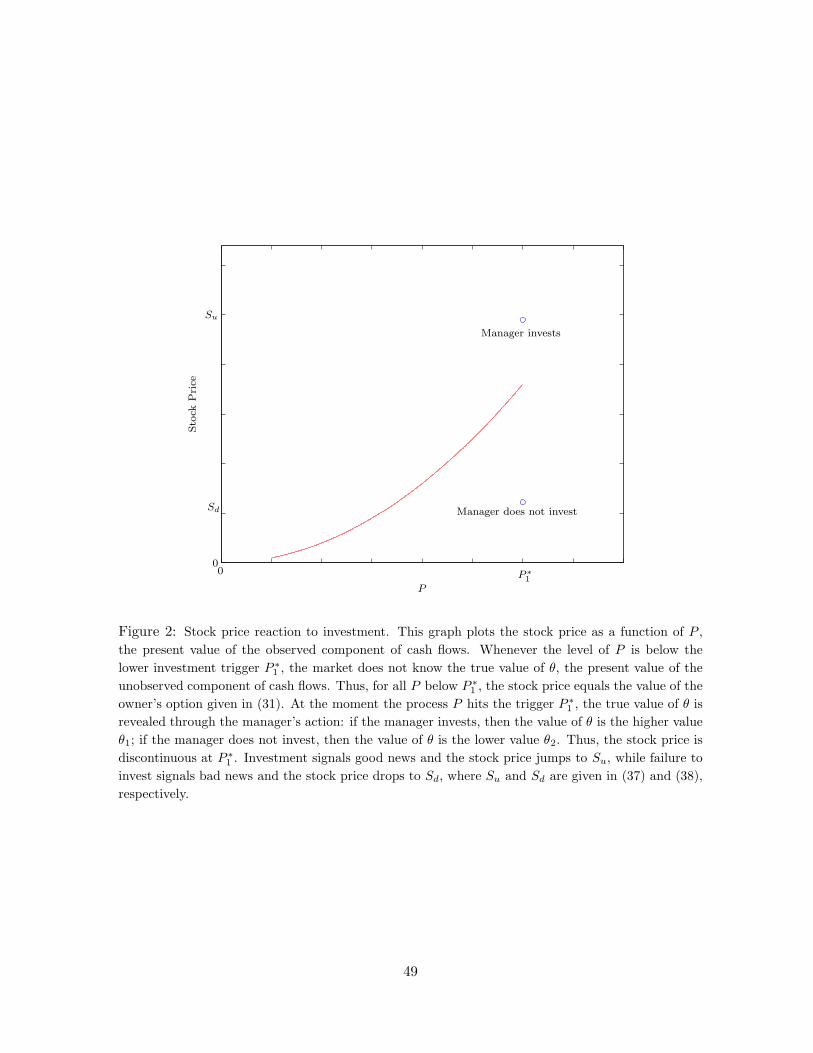
Figure 2 plots the stock price S as a function of P , the current value of the process P (t).

For all P < P ∗1 , S (P ) = πo (P ), where πo is given in (31). For P = P ∗

1 , S(P ) = Su if

investment is undertaken, and S(P ) = Sd if investment is not undertaken. The jump in29We thank the referee for suggesting this discussion.

22

the stock price at P ∗1 is a result of the information revealed by the manager’s investment

decisions.

This result is consistent with the empirical findings in McConnell and Muscarella (1985).

They find that announcements of unexpected increases in investment spending lead to in-

creases in stock prices, and ice versa for unexpected decreases.

Since the stock price movement at the trigger P ∗1 reveals the true value of θ, the manager’s

incentive contract can be made contingent on the stock price. For example, the manager

could be paid a bonus w1 if the stock price jumps upward to Su. Since w2 = 0, no bonus is

paid if the stock price falls to Sd. Similarly, such a contingent payoff could be implemented

through a properly parameterized stock option grant.

4.2 Agency Problems and Investment Lags

In the standard real options setting, investment is triggered at the value maximizing triggers,

P ∗1 and P ∗

2 , for the higher and lower project quality outcomes, respectively. However,

in our setting, while the trigger for investment in the higher quality state remains at P ∗1 ,

investment in the lower quality state may be triggered at PJ , which is higher than the first-

best benchmark level P ∗2 .

Let T and T ∗ be the stopping times at which the option is exercised, in our model and the

first-best setting, respectively. We denote Γ = E (T − T ∗) as the expected time lag due to the

principal-agent problem. A solution for such an expectation can be derived using Harrison

(1985, Chapter 3). The expected lag is given by

Γ =(

1 − qH

α − σ2/2

)ln(

PJ

P ∗2

)(39)

=(

1 − qH

α − σ2/2

)[ln(

P0

K − θ2

)+

1β

ln(

∆q∆θ

ξ

)− lnβ + ln (β − 1)

], (40)

where we assume that α > σ2/2 in order for this expectation to exist.

An important insight from Section 3 is that increases in the cost benefit ratio of inducing

effort lead to less distortion in investment timing. That is, as the ratio ξ/∆q increases, the

equilibrium trigger PJ becomes closer to the first-best trigger P ∗2 . This is confirmed by the

following comparative static:

∂Γ∂ (ξ/∆q)

= −(

1 − qH

α − σ2/2

)∆q

βξ< 0. (41)

23

An increase in the volatility of the underlying project, σ, has an ambiguous effect on the

expected time lag Γ. This can be seen from the following comparative static:

∂Γ∂σ

= −(

1 − qH

α − σ2/2

)1β2

[ln(

∆q∆θ

ξ

)− β

β − 1

]∂β

∂σ+

(1 − qH) σ

(α − σ2/2)2ln(

PJ

P ∗2

), (42)

where ∂β/∂σ < 0. An increase in σ raises the option value and makes waiting more worth-

while, implying that both P ∗2 and PJ are larger, ceteris paribus. However, if the cost benefit

ratio for exerting effort is relatively high, in that

ln(

ξ

∆q

)>

β − 1β

+ ln(∆θ), (43)

then the change of PJ relative to the change in P ∗2 is larger. Therefore, under such conditions

the expected time lag increases in volatility σ.

An increase in the expected growth rate of the project, α, also has an ambiguous effect

on the expected time lag Γ. This can be seen from the following comparative static:

∂Γ∂α

= − 1 − qH

(α − σ2/2)2

ln

(PJ

P ∗2

)− 1

β

(ln(

∆q∆θ

ξ

)− β

β − 1

)α − σ2/2√

(α − σ2/2)2 + 2rσ2

. (44)

However, if (43) holds, then expected time lag decreases with drift α.

4.3 Social Loss and Option Values

Although the owner chooses the value-maximizing contract to provide an incentive for the

manager to extend effort, the agency problem ultimately still proves costly. In an owner-

managed firm, the manager will extend effort and will exercise the option at the first-best

stopping time. However, in firms with delegated management, there will be a social loss due

to the firm’s suboptimal exercise strategy.

By a social loss, we are referring to the difference between the values of the first-best

option value, V ∗(P0) in (9), and the sum of the owner and manager options, πo(P0) and

πm(P0) in (31) and (32). Thus, define the social loss due to agency issues as L, where

L = V ∗(P0) − [πo(P0) + πm(P0)]. Simplifying, we have:

L = (1 − qH)

[(P0

P ∗2

)β

(P ∗2 − K + θ2) −

(P0

PJ

)β

(PJ − K + θ2)

]. (45)

This social loss is likely to have economic ramifications on the structure of firms. For firms

in industries with potentially large social losses due to agency costs, there will be powerful

24

forces that will push them to be privately held, or to be organized in a manner that provides

the closest alignment between owners and managers.

There are two effects of a later-than-first-best exercising trigger (PJ > P ∗2 ) on the social

loss L: (i) a larger payout (PJ + θ2 −K) reduces social loss, ceteris paribus, and (ii) a lower

discount factor [(P0/PJ )β < (P0/P∗2 )β] increases the social loss. The latter dominates the

former, because PJ > P ∗2 and P ∗

2 = arg max (P0/x)β (P0 + θ2 − K). Equation (45) suggests

that social loss is driven by the distance of the equilibrium trigger PJ from P ∗2 . As previously

discussed, the firm’s exercise timing becomes less distorted as the net cost benefit ratio of

inducing effort increases. That is, as the ratio ξ/∆q increases, the equilibrium trigger PJ gets

closer to the first-best trigger P ∗2 , and thus:

∂L

∂ (ξ/∆q)< 0. (46)

Note that with or without an agency problem, the owner’s value decreases as the cost

of effort ξ increases, in that dπo(P0)/dξ < 0. Without an agency problem (e.g., the firm’s

owner also manages the investment decisions), the owner’s value falls one for one with an

increase in effort cost; the owner simply must increase his effort outlay. In the case of

delegated management with agency costs, the owner’s value πo(P0 ) also falls as the cost of

effort increases. A question that we ask below is whether or not πo(P0 ) falls by more or less

than the first-best value does when the cost of effort increases.

In terms of the owner’s option value, the incentive problem represents a trade-off between

timing efficiency and the surplus that must be paid to the manager to extend effort. One can

obtain better intuition on the forces at work in the agency problem through the following

decomposition. In the first-best solution, the owner pays the cost of effort ξ and obtains the

first-best option value V ∗(P0). In the agency equilibrium, the owner delegates the cost of

effort to the manager, but then holds the sub-optimal option value πo(P0). The loss in the

owner’s option value due to the incentive problem is therefore given by

∆πo(P0) ≡ V ∗(P0) − ξ − πo(P0 ) = L + V m, (47)

where L is the total social loss given in (45), and V m is the ex-ante expected surplus paid to

the manager to exert effort, and is given by:

V m = πm(P0) − ξ = qHξ

∆q− ξ =

qL

∆qξ. (48)

25

Decomposing the loss in the owner’s option value given in (47) into the sum of the tim-

ing component (L) and the compensation component (V m) is useful for providing intuition.

When the owner delegates the option exercise decision to the manager, the owner’s option

value is lowered for two reasons: (i) the exercising inefficiency induced by agency and infor-

mation asymmetry; and (ii) the surplus needed to pay the manager to induce him to extend

effort and reveal his private information. The impact of a higher effort cost ξ represents a

trade-off in terms of the timing and compensation components. As shown in (46), a higher

effort cost results in more efficient investment timing. This must be traded-off against the

increased compensation that must be paid to provide appropriate incentives to the manager,

as seen in (48). Therefore, the total effect on the loss of owner’s option value due to an

increase in ξ depends on whether the “timing effect” or “compensation effect” is larger, in

that

∂

∂ξ∆πo(P0) = − (1 − qH) (β − 1)

(P0

PJ

)β (1 − P ∗

2

PJ

)PJ

βξ+

qL

∆q(49)

=β − 1

β

1∆q∆θ

[− (1 − qH) (PJ − P ∗2 ) + qL (P ∗

2 − P ∗1 )] . (50)

If the investment trigger PJ is significantly larger than P ∗2 , in that

(1 − qH) (PJ − P ∗2 ) > qL (P ∗

2 − P ∗1 ) , (51)

then an increase in ξ leads to a smaller loss in the owner’s option value, as the gain in timing

efficiency overshadows the loss due to the manager’s increased compensation.30 That is,

while the owner’s option value under agency falls as ξ increases, it may fall by less than the

full amount of the increase in ξ due to the gain in timing efficiency.

5 Impatient Managers and Early Investment

So far, we have assumed that both owners and managers value payoffs identically. However,

it may be the case that managers are more impatient than owners. There are several potential

justifications for such an assumption. First, there are various models of managerial myopia30Note that the above condition is non-empty. This can be seen as follows. Condition (51) is equivalent to

PJ >1

1 − qH[(1 − qH)P ∗

2 + qL(P ∗2 − P ∗

1 )] = P ∗3 − ∆q

1 − qH(P ∗

2 − P ∗1 ) .

The joint hidden action/hidden information region is characterized by P ∗2 ≤ PJ ≤ P ∗

3 . Therefore, the abovecondition is met for some PJ .

26

that attempt to explain a manager’s preference for choosing projects with quicker pay-backs,

even in the face of eschewing more valuable long-term opportunities. For example, Narayanan

(1985) and Stein (1989) argue that concerns about either the firm’s short-term performance or

labor-market reputation may give the manager an incentive to take actions that pay off in the

near term at the expense of the long term. Second, in our “investment timing” setting, greater

impatience can represent the manager’s preference for empire building or greater perquisite

consumption and reputation that comes from running a larger company sooner rather than

later. Third, managerial short-termism could be the result of the manager facing stochastic

termination.31 This termination, for example, could be due to the manager leaving for a

better job elsewhere or being fired. We can model such stochastic termination by supposing

that the manager faces an exogenous termination driven by a Poisson process with intensity

ζ. The addition of stochastic termination transforms the manager’s option to one in which

his discount rate r is elevated to r + ζ to reflect the stochastic termination.32

Phrased in real options terms, managerial impatience decreases the value of the manager’s

option to wait. Thus, this generalization leads to very different predictions about investment

timing. While the basic model predicts that investment will never occur earlier than the first-

best case, in this generalized setting investment can occur earlier or later than the first-best

case. This is similar to the result found in Stulz (1990) where there is – which generates?

both over- and under-investment in the capital allocation decision, as shareholders use debt

to constrain managerial empire-building preferences.

Recall that the owner discounts future cash flows by the discount function D(P0; P ) =(P0/P

)βfor P0 < P . We can therefore represent greater managerial impatience by defining a

managerial discount function Dm(P0; P ) =(P0/P

)γ, where γ > β ensures that Dm(P0; P ) <

D(P0; P ). That is, a dollar received at the stopping time described by the trigger strategy

P is worth less to the manager than to the owner.33

This generalized problem is quite similar to that of Section 2, with the exception that the

constraints all use γ rather than β. Much of the solution methodology is the same. For

example, Propositions 1 and 2 apply as before, using the same proof. In addition, Proposition31We assume that the owner can costlessly replace the manager in the event of separation.32We suppose that the manager receives his reservation value (normalized to zero), when the termination

occurs. See Yaari (1965), Merton (1971) and Richard (1975) for analogous results on stochastic horizon.33Note that this is also consistent with the interpretation that the manager has a higher discount rate than

the owner. Since ∂β/∂r > 0, the manager’s higher discount rate is embodied by the condition γ > β.

27

3 and 4 remain valid, and are demonstrated in Appendix C. Thus, the optimal contracting

problem in the generalized setting can be written as:

maxw1, P1, P2

qH

(P0

P1

)β

(P1 + θ1 −K)− qH

(P0

P1

)β

w1 + (1 − qH)(

P0

P2

)β

(P2 + θ2 −K), (52)

subject to(

P0

P1

)γ

w1 ≥(

P0

P2

)γ

∆θ , (53)(

P0

P1

)γ

w1 ≥ ξ

∆q. (54)

Similar to Proposition 5, at least one of (53) and (54) binds. Otherwise, the owner may strictly

increases his payoff by lowering the wage payment w1 without violating any constraints.

Just as in Section 3, there are three contracting regions: a hidden information region,

a joint hidden information/hidden action region, and a hidden action region, depending on

the level of cost/benefit ratio ξ/∆q. In this section, we focus on the joint hidden informa-

tion/hidden action region.34

The joint hidden information/hidden action region is defined by: (P0/P∗3 )γ∆θ < ξ/∆q <

(P0/P∗2 )γ∆θ, where P ∗

3 is defined in (C.11), and shown to be greater than the trigger P ∗2 . In

this region the optimal contract can be written as:

P1 = P1, (55)

P2 = PJ = P0

(∆q∆θ

ξ

)1/γ

, (56)

w1 =

(P1

PJ

)γ

∆θ < ∆θ, (57)

w2 = 0, (58)

where P1 is the root of H(x) = 0, defined by

H(x) =β

β − 1

[K − θ1 +

(1 − γ

β

)(x

P0

)γ ξ

∆q

]− x. (59)

Unlike the results of the basic model, we now have the possibility of investment occurring

before the first-best trigger is reached, in that P1 = P1 < P ∗1 . To see this, note that

H(0) = P ∗1 and

H(P ∗1 ) =

β

β − 1

(1 − γ

β

)(P ∗

1

P0

)γ ξ

∆q< 0. (60)

34The derivations for the optimal contracts in the other regions are shown in Appendix C.

28

The derivative of H( · ) is

H ′(x) =β

β − 1γ

(1 − γ

β

)(x

P0

)γ−1 1P0

ξ

∆q− 1 < 0. (61)

Therefore, there exists a unique solution P1 = P1 < P ∗1 .

As in the basic model, the trigger strategy for the manager of a θ2-type project is greater

than the first-best trigger, P ∗2 . Recall that PJ > P ∗

2 in the region (P0/P∗3 )γ∆θ < ξ/∆q <

(P0/P∗2 )γ∆θ, where P ∗

3 is given in (C.11). However, for γ > β, the trigger is closer to the

first-best trigger than for the standard case in which γ = β. This is true, since for γ > β,

PJ = P0

(∆q∆θ

ξ

)1/γ

< P0

(∆q∆θ

ξ

)1/β

= PJ . (62)

Thus, when the manager is more impatient than the owner, equilibrium investment occurs

sooner than it does in the standard principal-agent model described earlier in the paper. In

particular, investment actually occurs prior to the first-best trigger is reached for the θ1-type

project. The greater impatience on the part of the manager implies that it is in the owner’s

interest to offer a contract that motivates earlier exercise. This results in both costs and

benefits to the owner. By motivating investment for the θ2-type project earlier than the

standard principal-agent model, investment timing trigger moves closer to the first-best one.

Since the manager receives no surplus for the θ2-type project, the owner is the sole beneficiary

of this timing efficiency. However, investment for the θ1-type project occurs earlier than that

in the model of Section 2, which is the first-best outcome. Therefore, the owner is worse off

with respect to the θ1-type projects for two reasons: investment occurs too early, and the

wage paid to the manager in this state must be higher (than in the standard model) in order

to motivate earlier investment. The net effect on ex-ante owner’s option value is ambiguous

and is driven by the relative parameter values.

6 Conclusion

This paper extends the real options framework to account for the agency and information

issues that are prevalent in many real-world applications. When investment decisions are

delegated to managers, contracts must be designed to provide incentives for managers to

both extend effort and to truthfully reveal their private information. This paper provides a

model of optimal contracting in a continuous-time principal-agent setting in which there is

29

both moral hazard and adverse selection. The implied investment behavior differs significantly

from that of the first-best no-agency solution. In particular, there will be greater inertia in

investment, as the model predicts that the manager will have a more valuable option to wait

than the owner. The interplay between the twin forces of hidden information and hidden

action leads to markedly different investment outcomes than when only one of the two forces

is at work. Allowing the manager to have an effort choice that affects the likelihood of getting

a high quality project mitigates the investment inefficiency due to information asymmetry.

When the model is generalized to include differing degrees of impatience between owners and

managers, we find that investment may occur either earlier or later than optimal.

Some extensions of the model would prove interesting. First, the model could allow for

repeated investment decisions. This richer setting would permit owners to update their

beliefs over time, and for managers to establish reputations. Second, the model could also

be generalized to include competition in both the labor and product markets. As shown by

Grenadier (2002), the forces of competition greatly alter the investment behavior implied by

standard real options models.

30

Appendices

A Solution to the Optimal Contracting Problem

This appendix provides a derivation of the optimal contracts detailed in Section 3.

First, we simplify the optimal contracting problem by presenting and proving

the following four propositions. Proposition 1 shows that the limited liability

for the manager of a θ1-type project in constraint (19) does not bind, while

Proposition 2 shows that the ex-ante participation constraint (16) does not bind.

Proposition 1. The limited-liability condition for a manager of a θ1-type project does not

bind. That is, w1 > 0.

Proof.

w1 ≥(

P1

P2

)β

(w2 + ∆θ) ≥(

P1

P2

)β

∆θ > 0,

The first and second inequalities follow from (17) and (19), respectively.

In order to motivate the manager to exert effort, we need to reward the manager with

an option value larger than zero, which is the manager’s reservation value. This leads to the

following result.

Proposition 2. The ex-ante participation constraint (16) does not bind.

Proof. (P0

P1

)β

w1 +1 − qH

qH

(P0

P2

)β

w2 −ξ

qH≥ ξ

∆q− ξ

qH> 0,

where the first inequality follows from the ex-ante incentive constraint (15) and the limited

liability condition for the type-θ2 project.

Propositions 1 and 2 allow us to express the owner’s objective as maximizing the value

of his option, given in (13), subject to (15), (17), (18) and w2 ≥ 0. Using the method of

31

Kuhn-Tucker, we form the Lagrangian as follows:

L =(

P0

P1

)β

(P1 + θ1 − K − w1) +1 − qH

qH

(P0

P2

)β

(P2 + θ2 − K − w2)

+ λ1

[(P0

P1

)β

w1 −(

P0

P2

)β

(w2 + ∆θ)

]+ λ2

[(P0

P2

)β

w2 −(

P0

P1

)β

(w1 − ∆θ)

]

+ λ3

[(P0

P1

)β

w1 −(

P0

P2

)β

w2 −ξ

∆q

]+ λ4 w2, (A.1)

with corresponding complementary slackness conditions for the four constraints.

The first-order condition with respect to w1 gives

λ1 − λ2 + λ3 = 1 . (A.2)

The first-order condition with respect to w2 implies

(−λ1 + λ2 − λ3 −

1 − qH

qH

)(P0

P2

)β

+ λ4 = 0. (A.3)

Simplifying (A.3) gives λ4 = (P0/P2)β /qH > 0. Therefore, the complementary slackness

condition λ4 w2 = 0 implies that w2 = 0. This is summarized in Proposition 3.

Proposition 3. The limited liability for a manager of a θ2-type project binds, in that w2 = 0.

The intuition is straightforward. Giving the manager of a θ2-type project any positive

rents implies higher rents for managers of θ1-type projects in order to meet the ex-post

incentive constraint of the manager of a θ1-type project. In order to minimize the rents

subject to the manager’s participation and incentive constraints, the owner shall give the

manager of a θ2-type project no ex-post rents.

The first-order conditions with respect to P1 and P2 imply:

P1 =β

β − 1(K − θ1 − λ2∆θ) , (A.4)

P2 =β

β − 1

(K − θ2 +

qH

1 − qHλ1 ∆θ

). (A.5)

The following proposition states that the ex-post incentive constraint for the manager of

a θ2-type project, (18), does not bind, in that λ2 = 0. We verify this conjecture, formalized

in Proposition 4 for each region. Proposition 4 allows us to ignore (18) in the optimization

problem.

32

Proposition 4. Optimal contracts imply w1 ≤ ∆θ.

Intuitively, if w1 > ∆θ, then the manager of a θ2-type project would never accept the

equilibrium contract with w2 = 0. This would clearly be inconsistent with Proposition 3.

Propositions 1–4 jointly simplify the owner’s optimization problem as the solution to the

objective function (20), subject to constraints (21) and (22).

The following proposition demonstrates that at least one of the two constraints binds.

Proposition 5. At least one of (21) and (22) binds.

The argument is immediate. If Proposition 5 did not hold, then reducing w1 will increase

the owner’s value strictly without violating any of the constraints. With λ2 = 0, then (A.2)

may be written as λ1 + λ3 = 1. Therefore, it must be the case that at least one of (21) and

(22) binds.

The problem summarized in equations (20)-(22) is now solved below.

A.1 The Hidden Information Only Region

Suppose that the ex-ante incentive constraint (22) does not bind. Since (21) must hold as

an equality and λ1 = 1, (A.5) implies P2 = P ∗3 where P ∗

3 is given in (25) and w1 is given

in (26). The inequality P ∗1 < P ∗

3 implies (18) does not bind, consistent with Proposition 4.

Finally, in order to be consistent with the assumption that (22) does not bind, we require

that ξ/∆q < (P0/P∗3 )β ∆θ, the parameter range defining this hidden information only region.

A.2 The Joint Hidden Information/Hidden Action Region

We derive the optimal contract in this region by conjecturing that both (21) and (22) bind.

Solving these two equality constraints gives (29) and (30). The inequality PJ > P ∗1 confirms

that (18) does not bind, consistent with Proposition 4. The solution for P2 implies that λ1

can be written as:

λ1 =β − 1

β(PJ − P ∗

2 )1 − qH

qH∆θ. (A.6)

The only possible region under which both constraints may bind35 is characterized by(

P0

P ∗3

)β

∆θ <ξ

∆q<

(P0

P ∗2

)β

∆θ . (A.7)

35If (P0/P ∗1 )β∆θ > ξ/∆q > (P0/P ∗

2 )β∆θ, then only the third constraint binds. If (P0/P ∗3 )β∆θ > ξ/∆q,

then only the first constraint binds. If ξ/∆q > (P0/P ∗1 )β∆θ, then supporting high effort is no longer in the

owner’s interest.

33

We now show that indeed both (21) and (22) bind throughout this entire region. The region

characterized by (A.7) can be equivalently expressed as P ∗2 < PJ < P ∗

3 . Because (A.6)

implies that λ1 is monotonically increasing in PJ , therefore, 0 < λ1 < 1 in this region. Since

λ3 = 1−λ1, we also have 0 < λ3 < 1. By complementary slackness conditions, both (21) and

(22) bind in this joint region, confirming the result that (A.7) is the whole region, with both

constraints binding.36

A.3 The Hidden Action Only Region

Suppose that (21) does not bind and (22) binds, then λ1 = 0 by complementary slackness,

and λ3 = 1. Therefore, P2 = P ∗2 given in (33) and w1 is given in (34). We need to verify that

(21) and (18) do not bind. The constraint (18) is non-binding (consistent with Proposition

4) if and only if P ∗1 < PJ . The constraint (21) is non-binding if and only if PJ < P ∗

2 . Thus,

together these imply that P ∗1 < PJ < P ∗

2 , which is identical to the condition (P0/P∗2 )β∆θ <

ξ/∆q < (P0/P∗1 )β∆θ, that defines this region.

If the parameters do not fall in any of the three regions, namely, ξ/∆q > (P0/P∗1 )β∆θ

then it can be shown that the owner will not choose to motivate the manager to exert effort.

The cost of effort is so high as to overwhelm any potential benefits of motivating effort. A

proof of this result is available from the authors upon request.

B Optimal Contracting with a Continuous Distribution of θ

This appendix contains the derivation of the optimal contracts when the distribution of the

project’s unobserved component θ of value is continuous.

Denote the manager’s time-zero expected utility as u(θ, θ), if he reports that his privately

observed component of project value is θ, and the true level of his privately observed value

is θ. His time-zero expected utility is then given by

u(θ, θ) =

(P0

P (θ)

)β (w(θ) + θ − θ

). (B.1)

We denote U(θ) as the value function of the manager whose privately observed component36We also need additional technical conditions to ensure that inducing the manager to extend high effort is

in the interest of the owner.

34

of project value is θ. That is,

U(θ) = u(θ, θ) =(

P0

P (θ)

)β

w(θ). (B.2)

As in Section 2, we denote ξ as the cost of extending effort at time zero. Let FH(θ) and

FL(θ) be the cumulative distribution functions of θ drawn if the manager extends effort and

if he does not extend effort, respectively. Using the revelation principle, we may write the

principal’s optimization problem as follows:

maxP ( · ), w( · )

∫ θ

θ

(P0

P (θ)

)β

(P (θ) + θ − K − w(θ)) dFH(θ) , (B.3)

subject to:

1. ex-post incentive-compatibility condition:

U(θ) ≥ u(θ, θ) , for any θ and θ ; (B.4)

2. limited-liability condition:

w(θ) ≥ 0 , for any θ ; (B.5)

3. ex-ante incentive compatibility condition:

∫ θ

θU(θ) dFH(θ) − ξ ≥

∫ θ

θU(θ) dFL(θ) ; (B.6)

4. ex-ante participation constraint:

∫ θ

θU(θ) dFH(θ) − ξ ≥ 0. (B.7)

Proposition 6. The ex-ante participation constraint (B.7) does not bind.

Proof. The ex-ante incentive constraint (B.6) and the limited-liability condition (B.5) to-

gether imply that the ex-ante participation constraint (B.7) does not bind.

First, we simplify the ex-ante incentive constraint (B.6) using integration by parts. This

gives ∫ θ

θM(θ) dU(θ) ≥ ξ , (B.8)

where M(θ) = − (FH(θ) − FL(θ)) .

35

Next, we simplify the ex-post incentive-compatibility condition (B.4) by totally differen-

tiating U(θ), the value function for a manager of a type-θ project, with respect to θ. This

givesdU(θ)

dθ= u1

dθ

dθ+ u2 , (B.9)

where

u1 =∂u(θ, θ)

∂θ

∣∣∣∣θ=θ

, and u2 =∂u(θ, θ)

∂θ

∣∣∣∣θ=θ

. (B.10)

Since the manager optimally reveals his project quality by choosing recommended equilibrium

strategy, we have u1(θ, θ) = 0. Therefore, we have U ′(θ) = u2. Integration gives

U(θ) = U(θ) +∫ θ

θu2(s, s) ds = U(θ) +

∫ θ

θ

(P0

P (s)

)β

ds. (B.11)

We note that the Spence-Mirrlees condition is satisfied.37

A standard result in the contracting literature with asymmetric information states that the

limited-liability condition for a manager of a θ-type project binds, in that U(θ) = w(θ) = 0.

Therefore, the information rents U(θ) that accrues to the manager of a θ-type project is given

by

U(θ) =∫ θ

θ

(P0

P (s)

)β

ds . (B.12)

The relationship between U(θ) and the equilibrium wage implies that

w(θ) =(

P (θ)P0

)β

U(θ) =∫ θ

θ

(P (θ)P (s)

)β

ds. (B.13)

Using (B.13), we simplify the present value of expected wage payment as follows:

∫ θ

θ

(P0

P (θ)

)β

w(θ) dFH (θ) =∫ θ

θ

[∫ θ

θ

(P0

P (s)

)β

ds

]dFH(θ) ,

=

[∫ θ

θ

(P0

P (s

)β

ds

]FH(θ)

∣∣∣∣θ

θ

−∫ θ

θFH(θ)

(P0

P (θ)

)β

dθ ,

=∫ θ

θλH(θ)

(P0

P (θ)

)β

dFH(θ), (B.14)

where

λH(θ) =1 − FH(θ)

fH(θ)(B.15)

is the inverse of the hazard rate under FH( · ).37Details are available upon request.

36

Using (B.14) allows us to simplify the principal’s optimization problem as follows:

maxP ( · )

∫ θ

θ

(P0

P (θ)

)β

(P (θ) + θ − K − λH(θ)) dFH(θ) , (B.16)

subject to the ex-ante incentive constraint (B.8) and ex-post limited-liability condition (B.5).

The equilibrium wage is then obtained by using (B.13).

Similar to the model with discrete values for θ, optimal contracts, characterized by the

pair of trigger strategy and wage payment functions, depend on the region in which effort

cost ξ lies. Subsection B.1 solves for the optimal contracts in the region under which the

ex-ante incentive constraint does not bind. Subsection B.2 solves for the optimal contracts

in the region under which both the ex-ante incentive constraint and the ex-post incentive

constraint bind.

B.1 The Hidden Information Only Region

If effort cost ξ is low enough, then no additional rent is needed to induce the manager to

extend effort. The following condition ensures that the ex-ante incentive constraint (B.8)

does not bind.

Condition 1. ∫ θ

θM(θ)

(P0

P ∗3 (θ)

)β

dθ ≥ ξ, (B.17)

where

P ∗3 (θ) =

β

β − 1[K − θ + λH(θ)] . (B.18)

Maximizing (B.16) may be done point by point. This gives the candidate optimal trigger

level P (θ) = P ∗3 (θ), where P ∗

3 (θ) is given in (B.18). Because λH(θ) > 0, the exercise trigger

is larger than the first-best level, confirming the intuition delivered in Section 3 using the

two-point distribution of θ. A verification easily confirms that (B.8) does not bind under

Condition 1.

The following condition ensures that the candidate trigger strategy is positive for any θ.

Condition 2. For all θ on the support, θ − λH(θ) < K .

Finally, we ensure that the candidate trigger strategy decreases in θ by requiring the

following condition:

37

Condition 3. dλH(θ)/dθ < 1.

It is straightforward to note that Conditions 2 and 3 also imply that wage is positive and

increases in the project quality θ, as seen from (B.13).

B.2 The Joint Hidden Information/Hidden Action Region

When the effort cost is higher, both the ex-ante incentive constraint (B.6) and the ex-post

incentive constraint (B.4) bind. The condition governing the parameters for this region when

θ is drawn from a continuous distribution is given as follows.

Condition 4.∫ θ

θM(θ)

(P0

P ∗3 (θ)

)β

dθ ≤ ξ ≤∫ θ

θM(θ)

(P0

P ∗2 (θ)

)β

dθ , (B.19)

where P ∗3 (θ) is given in (B.18) and

P ∗2 (θ) =

β

β − 1

(K − θ +

1 − FL(θ)fH(θ)

). (B.20)

Denote l as the Lagrangian multiplier for (B.8). Then, the candidate equilibrium trigger

strategy is given by

P (θ) = PJ(θ) =β

β − 1

(K − θ + λH(θ) − l

M(θ)fH(θ)

). (B.21)

The Lagrangian multiplier l is positive under Condition 4. Therefore, the optimal trigger

with the exception of the one for the manager of the lowest quality project θ is larger than

the first-best P ∗(θ) = β(K − θ)/(β − 1). Because (B.8) holds with strict equality, we may

combine (B.8), (B.12) and (B.21) in order to obtain

ξ =∫ θ

θM(θ)

(P0

PJ(θ)

)β

dθ . (B.22)

Solving the above equation gives the Lagrangian multiplier l. It is straightforward to show

that the Lagrangian multiplier l increases in effort cost ξ, in that

dl

dξ=

P0

β − 1

[∫ θ

θ

M2(θ)fH(θ)

(β

β − 1

)2 ( P0

PJ(θ)

)β+1

dθ

]−1

. (B.23)

Therefore, as effort cost ξ increases, the optimal trigger PJ(θ) decreases, as shown below:

dPJ(θ)dξ

= − β

β − 1M(θ)fH(θ)

dl

dξ< 0. (B.24)

38

This is consistent with our intuition and results in Section 3 that a higher effort cost mitigates

investment inefficiency by pushing the exercise trigger towards the first-best level.

The following two conditions ensure that the conjectured candidate solutions PJ(θ) is

positive and decreasing in θ.

Condition 5.d

dθ

(θ − λH(θ) + l

M(θ)fH(θ)

)> 0 , (B.25)

for 0 ≤ l ≤ 1.

Condition 6. The distribution FH( · ) first-order stochastically dominates FL( · ), in that

FH(θ) ≤ FL(θ), for all θ . (B.26)

This implies M(θ) ≥ 0, for all θ.

We note that, under Conditions 5 and 6, wage is positive and increasing in θ, in that

w(θ2) =∫ θ

θ2

(P (θ2)P (s)

)β

ds >

∫ θ2

θ

(P (θ1)P (s)

)β

ds >

∫ θ1

θ

(P (θ1)P (s)

)β

ds = w(θ1) , (B.27)

for θ2 > θ1. The first inequality follows from the monotonicity of P (θ).

C Derivations of Optimal Contracts in Section 5

This appendix provides a derivation of the optimal contracts for the generalized model of

Section 5. Propositions 1 and 2 apply as in Appendix A. Using the method of Kuhn-Tucker,

we form the Lagrangian as follows:

L =(

P0

P1

)β

(P1 + θ1 − K − w1) +1 − qH

qH

(P0

P2

)β

(P2 + θ2 − K − w2)

+ λ1

[(P0

P1

)γ

w1 −(

P0

P2

)γ

(w2 + ∆θ)]

+ λ2

[(P0

P2

)γ

w2 −(

P0

P1

)γ

(w1 − ∆θ)]

+ λ3

[(P0

P1

)γ

w1 −(

P0

P2

)γ

w2 −ξ

∆q

]+ λ4 w2 , (C.1)

with corresponding complementary slackness conditions for the four constraints. As in Ap-

pendix A, we also conjecture that the ex-post incentive constraint does not bind, in that the

Lagrangian multiplier λ2 associated with the constraint below is zero:(

P0

P2

)γ

w2 ≥(

P0

P1

)γ

(w1 − ∆θ) . (C.2)

39

We will verify this conjecture for each region.

The first-order conditions with respect to w1 and w2 imply

0 = (λ1 + λ3)(

P0

P1

)γ

−(

P0

P1

)β

, (C.3)

0 = − (λ1 + λ3)(

P0

P2

)γ

− 1 − qH

qH

(P0

P2

)β

+ λ4 . (C.4)

Using (C.3) to simplify (C.4) gives λ4 > 0. The complementary slackness condition implies

that w2 = 0. The first-order conditions with respect to P1 and P2 are given by

P1 =β

β − 1

[K − θ1 +

(1 − γ

β

)w1

], (C.5)

P2 =β

β − 1

[K − θ2 + λ1

qH

1 − qH

γ

β

(P0

P2

)γ−β

∆θ

]. (C.6)

Therefore, it must be the case that at least one of (53) and (54) binds (Similar to Proposition

5 of Appendix A). Depending on the cost benefit ratio ξ/∆q, we have three disjoint regions

to be analyzed below, similar to the analyses in Section 3.

C.1 The Hidden Information Only Region

Suppose that the constraint (54) does not bind and thus λ3 = 0. Then, λ1 = (P0/P1)β−γ >

1. A binding ex-ante incentive constraint (53) implies that the wage payment is w1 =

(P1/P2)γ ∆θ . The first-order conditions (C.5) and (C.6) give the following coupled equa-

tions:

P1 =β

β − 1

[K − θ1 +

(1 − γ

β

)(P1

P2

)γ

∆θ

], (C.7)

P2 =β

β − 1

[K − θ2 +

qH

1 − qH

γ

β

(P1

P2

)γ−β

∆θ

]. (C.8)

Note that with γ > β, we immediately have P1 < P ∗1 and P2 > P ∗

2 . Therefore, w1 < ∆θ, as

conjectured, confirming that (C.2) does not bind and λ2 = 0.

Define the ratio x = P1/P2. The coupled equations (C.7) and (C.8) allow us to first solve

for ratio x∗, in that

G(x∗) = 0, (C.9)

where

G(x) = x

[K − θ2 +

γ

β

(qH

1 − qH

)xγ−β∆θ

]−[K − θ1 +

(1 − γ

β

)xγ∆θ

]= 0. (C.10)

40

First, note that G(0) = −(K − θ1) < 0 and G(1) = γ∆θ/(β(1 − qH)) > 0. Second,

G′(x) = K − θ2 +γ + γ(γ − β)

β

qH

1 − qHxγ−β∆θ + γxγ−1

(γ

β− 1)

∆θ > 0 ,

for γ > β. Therefore, there exist a unique x∗ ∈ (0, 1) solving (C.9).

Therefore, for the region defined by ξ/∆q < (P/P ∗3 )γ∆θ, where

P ∗3 =

β

β − 1

[K − θ2 +

qH

1 − qH

γ

β(x∗)γ−β∆θ

], (C.11)

the optimal contract can be written as:

P1 =β

β − 1

[K − θ1 +

(1 − γ

β

)(x∗)γ ∆θ

], (C.12)

P2 = P ∗3 , (C.13)

w1 =(

P1

P2

)γ

∆θ, (C.14)

w2 = 0. (C.15)

Finally, if ξ/∆q < (P0/P∗3 )γ∆θ, constraint (54) is indeed not binding, consistent with our

conjecture.

C.2 The Joint Hidden Information/Hidden Action Region

We derive the optimal contract in this region by conjecturing that both (53) and (54) bind.

Solving these two equality constraints gives (56) and (57). Plugging (56) and (57) into the

first-order condition (C.5) gives

P1 =β

β − 1

[K − θ1 +

(1 − γ

β

)(P1

PJ

)γ

∆θ

]. (C.16)

The solution for P1 is P1, the same solution for P1 as in the hidden action region. In

Section 5 we proved that a unique P1 exists, where P1 ∈ (0, P ∗1 ). Naturally, we have

w1 =(P1/PJ

)γ∆θ. As before, we have verified that (C.2) does not bind in this region,

because P1 < PJ implies that w1 < ∆θ.

We know that the only possible regions in which both (53) and (54) bind is (P0/P∗3 )γ∆θ ≤

ξ/∆q ≤ (P0/P∗2 )γ∆θ, since we have already shown that in the other regions only one of

these constraints binds.38 Equivalently stated in terms of PJ , this region is characterized by

38Note that in the region ξ/∆q > (P0/P1)γ∆θ, it can be shown that effort cannot be induced. This result

is available upon request.

41

P ∗2 < PJ < P ∗

3 . We now verify that the above solutions are indeed optimal for this entire

region. Recall that λ1 + λ3 =(P0/P1

)β−γ. Therefore, if we show that λ1 lies within the

range defined by

0 < λ1 <

(P0

P1

)β−γ

, (C.17)

then we have shown both (53) and (54) bind (λ1, λ3 6= 0).

The first-order condition with respect to P2 implies that

λ1 =

[β

β − 1qH

1 − qH

γ

β

(P0

PJ

)γ−β

∆θ

]−1 (PJ − P ∗

2

). (C.18)

Since PJ > P ∗2 , we have confirmed that λ1 > 0. We next prove that λ1 <

(P0/P1

)β−γ.

Expressing λ1 as a function of PJ , we can rewrite (C.18) as:

λ1(PJ ) =

(P0

P1(PJ)

)β−γ (P1(PJ )

PJ

)β−γ [qH

1 − qH

γ

β(P ∗

2 − P ∗1 )]−1 (

PJ − P ∗2

). (C.19)

Note that from (C.16), P1 is a function of PJ ; we make this functional dependence explicit

in the above equation. Proving that λ1 <(P0/P1

)β−γover the region PJ ∈ (P ∗

2 , P ∗3 ) is

equivalent to showing that

N(x) > 0, for x ∈ (P ∗2 , P ∗

3 ),

where N(x) is defined by

N(x) = P ∗2 +

(P1(x)

x

)γ−βqH

1 − qH

γ

β(P ∗

2 − P ∗1 ) − x. (C.20)

Using implicit differentiation in (C.16), we can write:

dP1(x)dx

=P1(x)

x

γ(P1(x) − P ∗1 )

γ(P1(x) − P ∗1 ) − P1(x)

> 0, (C.21)

because P1(x) < P ∗1 in this region. Therefore,

dL(x)dx

= (γ − β)qH

1 − qH

γ

β(P ∗

2 − P ∗1 )

(P1(x)

x

)γ−β−11x2

(x

dP1(x)dx

− P1(x)

)− 1 . (C.22)

From (C.21),

xdP1(x)

dx− P1(x) =

(P1(x)

)2

γ(P1(x) − P ∗1 ) − P1(x)

< 0, (C.23)

because P1(x) < P ∗1 in this region. Therefore, N ′(x) < 0, for x ∈ (P ∗

2 , P ∗3 ). Since N(P ∗

3 ) = 0,

we thus have N(x) > 0 for x ∈ (P ∗2 , P ∗

3 ). This confirms that λ1, λ3 > 0 in this entire region,

and therefore both (53) and (54) bind.

42

C.3 The Hidden Action Only Region

Suppose that (54) binds, while (53) does not. Thus, λ1 = 0 and λ3 = (P0/P1)β−γ > 1. With

λ1 = 0, equation (C.6) implies that P2 = P ∗2 .

A binding (54) implies that the wage payment is

w1 =(

P1

P0

)γ ξ

∆q=(

P1

PJ

)γ

∆θ, (C.24)

where PJ is given in (56). Substituting (C.24) into (C.5) gives P1 = P1, the root of the

expression given in (59). Section 5 proves that a unique P1 exists, where P1 ∈ (0, P ∗1 ).

To ensure that our conjecture that (C.2) is not binding, (C.24) implies that we need to

check if P1 < PJ holds. This inequality can be written as ξ/∆q < (P0/P1)γ∆θ, which is

assured to hold in this region. In order to be consistent with the fact that (53) does not bind,

we need (P0/P∗2 )γ∆θ > ξ/∆q, which again holds in this region.

43

References

[1] Antle, R., and G. Eppen, 1985, “Capital Rationing and Organizational Slack in Capital

Budgeting,” Management Science 31, 163-174.

[2] Bebchuk, L. A. and Lars Stole, 1993, “Do Short-Term Managerial Objectives Lead to

Under- or Over-Investment in Long-Term Projects?,” Journal of Finance 48, 719-29.

[3] Bernardo, A. E., H. Cai, and J. Luo, 2001, “Capital Budgeting and Compensation with

Asymmetric Information and Moral Hazard,” Journal of Financial Economics 61, 311-

344.

[4] Bjerksund, P., and G. Stensland, 2000, “A Self-Enforced Dynamic Contract for Process-

ing of Natural Resources,” in M. J. Brennan and L. Trigeorgis, eds, Project Flexibility,

Agency, and Competition, Oxford University Press.

[5] Bolton, P., and D. S. Scharfstein, 1990, “A Theory of Predation Based on Agency

Problems in Financial Contracting,” American Economic Review 80, 93-106.

[6] Brennan, M. J., 1990, “Latent Assets,” Journal of Finance 45, 709-730.

[7] Brennan, M. J., and E. Schwartz, 1985, “Evaluating Natural Resource Investments,”

Journal of Business 58, 135-157.

[8] Diamond, D., 1984, “Financial Intermediation and Delegated Monitoring,” Review of

Economic Studies 51, 393-414.

[9] Dixit, A., 1989, “Entry and Exit Decisions Under Uncertainty,” Journal of Political

Economy 97, 620-638.

[10] Dixit, A. K., and R. S. Pindyck, 1994, “Investment Under Uncertainty,” Princeton Uni-

versity Press, Princeton, New Jersey.

[11] Grenadier, S. R., 2002, “Option Exercise Games: An Application to the Equilibrium

Investment Strategies of Firms,” Review of Financial Studies 15, 691-721.

[12] Gale, D, and M. Hellwig 1985, “Incentive-compatible Debt Contracts: The One-period

Problem,” Review of Economic Studies 52, 647-63.

44

[13] Harris, M., C. H. Kriebel, and A. Raviv, 1982, “Asymmetric Information, Incentives and

Intrafirm Resource Allocation,” Management Science 28, 604-620.

[14] Harris, M., and A. Raviv, 1996, “The Capital Budgeting Process: Incentives and Infor-

mation” Journal of Finance 46, 297-355.

[15] Holmstrom, B. R. and J. Ricart i Costa, 1986, “Managerial Incentives and Capital

Management,” Quarterly Journal of Economics 101, 835-860.

[16] Innes, R. D., 1990, “Limited Liabilities and Incentive Contracting with ex-ante Action

Choices,” Journal of Economic Theory 52, 45-67.

[17] Jewitt, I., 1988, “Justifying the First-Order Approach to Principal-Agent Problems,”

Econometrica 56, 1170-1190.

[18] Leland, H. E., 1998, “Agency Costs, Risk Management, and Capital Structure,” Journal

of Finance 53, 1213-1243.

[19] Maeland, J., 2002, “Asymmetric Information About a Constant Investment Cost,” work-

ing paper, Norwegian School of Economics.

[20] Majd, S., and R. Pindyck, 1987, “Time to Build, Option Value, and Investment Deci-

sions,” Journal of Financial Economics 18, 7-28.

[21] Mauer D. C., and S. H. Ott, 2000, “Agency Costs, Underinvestment, and Optimal

Capital Structure: The Effect of Growth Options to Expand,” in M. J. Brennan and L.

Trigeorgis, eds, Project Flexibility, Agency, and Competition, Oxford University Press.

[22] Mauer D. C., and A. Triantis, 1994, “Interactions of Corporate Financing and Investment

Decisions: A Dynamic Framework,“,Journal of Finance 49, 1253-1277.

[23] McConnell J. J., and C. J. Muscarella, 1985, “Corporate Capital Expenditure Decisions

and the Market Value of the Firm,” Journal of Financial Economics 14, 399-422.

[24] Mello A., and J. Parsons, 1992, “Measuring the Agency Costs of Debt,” Journal of

Finance 47, 1887-1904.

[25] McDonald, R., and D. Siegel, 1986, “The Value of Waiting to Invest,” Quarterly Journal

of Economics 101, 707-727.

45

[26] Merton, R. C., 1973, “Theory of Rational Option Pricing,” Bell Journal of Economics

and Management Science 4, 141-183.

[27] Merton, R. C., 1971, “Optimal Consumption and Portfolio Rules in a Continuous-Time

Model,” Journal of Economic Theory 3, 373-413.

[28] Mirrlees, J., 1976, “The Optimal Structure of Incentives and Authority Within an Or-

ganization,” Bell Journal of Economics 7, 105-131.

[29] Morellec, E., 2001, “Asset Liquidity, Capital Structure and Secured Debt,” Journal of

Financial Economics 61, 173-206.

[30] Morellec, E., 2003, “Can Managerial Discretion Explain Observed Leverage Ratios?”

Manuscript, University of Rochester, forthcoming, Review of Financial Studies.

[31] Narayanan, M. P., 1985, “Managerial Incentives for Short-Term Results,” Journal of

Finance 40, 1469-1484.

[32] Paddock, J. L., D. R. Siegel, and J. L. Smith, 1988, “Option Valuation of Claims on

Real Assets: The Case of Offshore Petroleum Leases,” Quarterly Journal of Economics

103, 479-508.

[33] Richard, S., 1975, “Optimal Consumption, Portfolio, and Life Insurance Rules for an Un-

certain Lived Individual in a Continuous-Time Model,” Journal of Financial Economics

2, 187-204.

[34] Rogerson, W., “The First-Order Approach to Principal-Agent Problems,” Econometrica

53, 1357-1367.

[35] Stein, J. C., 1989, “Efficient Capital Markets, Inefficient Firms: A Model of Myopic

Corporate Behavior, ” Quarterly Journal of Economics 104, 655-669.

[36] Stein, J. C., 2001, “Agency, Information and Corporate Investment,” Manuscript, Har-

vard University.

[37] Stulz, R. M., 1990, “Managerial Discretion and Optimal Financing Policies,” Journal of

Financial Economics 26, 3-27.

46

[38] Titman, S., 1985, “Urban Land Prices Under Uncertainty,” American Economic Review

75, 505-514.

[39] Townsend, R., 1979, “Optimal Contracts and Competitive Markets with Costly State

Verification,” Journal of Economic Theory 21, 417-25.

[40] Triantis, A., and J. Hodder, 1990, “Valuing Flexibility as a Complex Option,” Journal

of Finance 45, 549-565.

[41] Trigeorgis, L., 1996, “Real Options,” MIT Press, Cambridge, MA.

[42] Williams, J. T., 1991, “Real Estate Development as an Option,” Journal of Real Estate

Finance and Economics 4, 191-208.

[43] Yaari M. E., 1965, “Uncertain Lifetime, Life Insurance, and the Theory of the Con-

sumer,” Review of Economic Studies 32, 137-150.

47

0

0

P ∗2

Effort Cost ξ

Effort Cost ξ

Equilib

rium

Wage

w1

Equilib

rium

Tri

gger

P2

Hidden Information

Hidden Information

Joint Region

Joint Region

Hidden Action

Hidden Action

Figure 1: Optimal incentive contracts across the three parameter regions. The upper and lower graphsplot the equilibrium trigger strategy P2 and wage payment w1 in terms of effort cost ξ, respectively.As the cost of effort increases, the hidden action problem becomes more pronounced. The upper graphdemonstrates that as the cost of effort increases, the equilibrium trigger strategy P2 decreases, as itapproaches the first best trigger P ∗

2 . The lower graph demonstrates that as the cost of effort increases,the wage payment must increase in order to induce effort from the manager. In summary, as the costof inducing hidden effort increases, the timing of investment becomes more efficient while the value ofthe compensation package increases.

48

00

Su

Sd

P ∗1

P

Sto

ckP

rice

Manager invests

Manager does not invest

Figure 2: Stock price reaction to investment. This graph plots the stock price as a function of P ,the present value of the observed component of cash flows. Whenever the level of P is below thelower investment trigger P ∗

1 , the market does not know the true value of θ, the present value of theunobserved component of cash flows. Thus, for all P below P ∗

1 , the stock price equals the value of theowner’s option given in (31). At the moment the process P hits the trigger P ∗

1 , the true value of θ isrevealed through the manager’s action: if the manager invests, then the value of θ is the higher valueθ1; if the manager does not invest, then the value of θ is the lower value θ2. Thus, the stock price isdiscontinuous at P ∗

1 . Investment signals good news and the stock price jumps to Su, while failure toinvest signals bad news and the stock price drops to Sd, where Su and Sd are given in (37) and (38),respectively.

49