Interest in this area of potential human hazard stems, in part, from the magnitude of harm or damage that an individual who is exposed can experience. It is widely known that the risks associated with exposures to ionizing radiation are significantly greater than compa-rable exposures to non-ionizing radiation. This fact notwithstanding, it is steadily becom-ing more widely accepted that non-ionizing radiation exposures also involve risks to which one must pay close attention. This chapter will focus on the fundamental characteristics of the various types of ionizing and non-ionizing radiation, as well as on the factors, parame-ters, and relationships whose application will permit accurate assessments of the hazard that might result from exposures to any of these physical agents.
RELEVANT DEFINITIONS
Electromagnetic Radiation
Electromagnetic Radiation refers to the entire spectrum of photonic radiation, from wave-lengths of less than 10–5 Å (10–15 meters) to those greater than 108 meters — a dynamic wavelength range of more than 22+ decimal orders of magnitude! It includes all of the segments that make up the two principal sub-categories of this overall spectrum, which are the “Ionizing” and the “Non-Ionizing” radiation sectors. Photons having wavelengths shorter than 0.4 µ (400 nm or 4,000 Å) fall under the category of Ionizing Radiation; those with longer wavelengths will all be in the Non-Ionizing group. In addition, the overall Non-Ionizing Radiation sector is further divided into the following three sub-sectors:
Optical Radiation Band * 0.1 µ to 2,000 µ, or 0.0001 to 2.0 mm
Radio Frequency/Microwave Band 2.0 mm to 10,000,000 mm, or 0.002 to 10,000 m
Sub-Radio Frequency Band 10,000 m to 10,000,000+ m, or 10 km to 10,000+ km
* It must be noted that the entirety of the ultraviolet sector [0.1 µ to 0.4 µ wave-lengths] is listed as a member of the Optical Radiation Band, and appears, there-fore, to be a Non-Ionizing type of radiation. This is not true. UV radiation is in-deed ionizing; it is just categorized incorrectly insofar as its group membership among all the sectors of Electromagnetic Radiation.
Although the discussion thus far has focused on the wavelengths of these various bands, this subject also has been approached from the perspective of the frequencies involved. Not surprisingly, the dynamic range of the frequencies that characterize the entire Electromag-netic Radiation spectrum also covers 22+ decimal orders of magnitude — ranging from 30,000 exahertz or 3 ×10 22 hertz [for the most energetic cosmic rays] to approximately 1 or 2 hertz [for the longest wavelength ELF photons]. The energy of any photon in this overall spectrum will be directly proportional to its wavelength — i.e., photons with the highest frequency will be the most energetic.
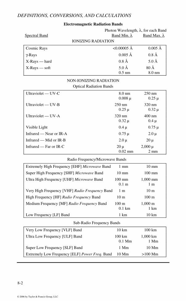
The most common Electromagnetic Radiation bands are shown in a tabular listing on the following page. This tabulation utilizes increasing wavelengths, or λs, as the basis for identifying each spectral band.
Ionizing Radiation is any photonic (or particulate) radiation — either produced naturally or by some man-made process — that is capable of producing or generating ions. Only the shortest wavelength [highest energy] segments of the overall electromagnetic spectrum are capable of interacting with other forms of matter to produce ions. Included in this grouping are most of the ultraviolet band [even though this band is catalogued in the Non-Ionizing sub-category of Optical Radiation], as well as every other band of photonic radiation having wavelengths shorter than those in the UV band.
Ionizations produced by this class of electromagnetic radiation can occur either “directly” or “indirectly.” “Directly” ionizing radiation includes:
(1) electrically charged particles [i.e., electrons, positrons, protons, α-particles, etc.], & (2) photons/particles of sufficiently great kinetic energy that they produce ionizations by
colliding with atoms and/or molecules present in the matter.
In contrast, “indirectly” ionizing particles are always uncharged [i.e., neutrons, photons, etc.]. They produce ionizations indirectly, either by:
(1) liberating one or more “directly” ionizing particles from matter with which these par-ticles have interacted or are penetrating, or
(2) initiating some sort of nuclear transition or transformation [i.e., radioactive decay, fission, etc.] as a result of their interaction with the matter through which these parti-cles are passing.
Protection from the adverse effects of exposure to various types of Ionizing Radiation is an issue of considerable concern to the occupational safety and health professional. Certain types of this class of radiation can be very penetrating [i.e., γ-Rays, X-Rays, & neutrons]; that is to say these particles will typically require very substantial shielding in order to en-sure the safety of workers who might otherwise become exposed. In contrast to these very penetrating forms of Ionizing Radiation, α- and β-particles are far less penetrating, and therefore require much less shielding.
Categories of Ionizing Radiation
Cosmic Radiation
Cosmic Radiation [cosmic rays] makes up the most energetic — therefore, potentially the most hazardous — form of Ionizing Radiation. Cosmic Radiation consists primarily of high speed, very high energy protons [protons with velocities approaching the speed of light] — many or even most with energies in the billions or even trillions of electron volts. These particles originate at various locations throughout space, eventually arriving on the earth after traveling great distances from their “birthplaces.” Cataclysmic events, or in fact any event in the universe that liberates large amounts of energy [i.e., supernovae, quasars, etc.], will be sources of Cosmic Radiation. It is fortunate that the rate of arrival of cosmic rays on Earth is very low; thus the overall, generalized risk to humans of damage from cos-mic rays is also relatively low.
Nuclear Radiation Nuclear Radiation is, by definition, terrestrial radiation that originates in, and emanates from, the nuclei of atoms. From one perspective then, this category of radiation probably should not be classified as a subset of electromagnetic radiation, since the latter is made up of photons of pure energy, whereas Nuclear Radiation can be either energetic photons or particles possessing mass [i.e., electrons, neutrons, helium nuclei, etc.]. It is clear, however,
that this class of “radiation” does belong in the overall category of Ionizing Radiation; thus it will be discussed here. In addition, according to Albert Einstein’s Relativity Theory, en-ergy and mass are equivalent — simplistically expressed as E = mc2 — this fact further so-lidifies the inclusion of Nuclear Radiation in this area.
Nuclear events such as radioactive decay, fission, etc. all serve as sources for Nuclear Ra-diation. Gamma rays, X-Rays, alpha particles, beta particles, protons, neutrons, etc., as stated on the previous page, can all be forms of Nuclear Radiation. Cosmic rays should also be included as a subset in this overall category, since they clearly originate from a wide variety of nuclear sources, reactions, and/or disintegrations; however, since they are extra-terrestrial in origin, they are not thought of as Nuclear Radiation. Although of interest to the average occupational safety and health professional, control and monitoring of this class of ionizing radiation usually falls into the domain of the Health Physicist.
Gamma Radiation
Gamma Radiation — Gamma Rays [γ-Rays] — consists of very high energy photons that have originated, most probably, from one of the following four sources:
(1) nuclear fission [i.e., the explosion of a simple “atomic bomb,” or the reactions that occur in a power generating nuclear reactor],
(2) nuclear fusion [i.e., the reactions that occur during the explosion of a fusion based “hydrogen bomb,” or the energy producing mechanisms of a star, or the operation of one of the various experimental fusion reaction pilot plants, the goal of which is the production of a self-sustaining nuclear fusion-based source of power],
(3) the operation of various fundamental particle accelerators [i.e., electron linear ac-celerators, heavy ion linear accelerators, proton synchrotrons, etc.], or
(4) the decay of a radionuclide.
While there are clearly four well-defined source categories for Gamma Radiation, the one upon which we will focus will be the decay of a radioactive nucleus. Most of the radioac-tive decays that produce γ-Rays also produce other forms of ionizing radiation [β–-particles, principally]; however, the practical uses of these radionuclides rest mainly on their γ-Ray emissions. The most common application of this class of isotope is in the medical area. Included among the radionuclides that have applications in this area are: 53
125 I & 53
131 I [both
used in thyroid therapy], and 27
60 Co [often used as a source of high energy γ-Rays in radia-
tion treatments for certain cancers]. Gamma rays are uncharged, highly energetic photons possessing usually 100+ times the energy, and less than 1% of the wavelength, of a typical X-Ray. They are very penetrating, typically requiring a substantial thickness of some shielding material [i.e., lead, steel rein-forced concrete, etc.].
Alpha Radiation
Alpha Radiation — Alpha Rays [α-Rays, α-particles] — consists solely of the completely ionized nuclei of helium atoms, generally in a high energy condition. As such, α-Rays are particulate and not simply pure energy; thus they should not be considered to be electro-magnetic radiation — see the discussion under the topic of Nuclear Radiation, beginning on the previous page.
These nuclei consist of two protons and two neutrons each, and as such, they are among the heaviest particles that one ever encounters in the nuclear radiation field. The mass of an α-particle is 4.00 atomic mass units, and its charge is +2 [twice the charge of the electron, but positive — the basic charge of an electron is –1.6 × 10⁻¹⁹ coulombs]. The radioactive de-
cay of many of the heaviest isotopes in the periodic table frequently involves the emission of α-particles. Among the nuclides included in this grouping are: 92
238 U , 88
226 Ra , and 86
222 Rn .
Considered as a member of the nuclear radiation family, the α-particle is the least penetrat-ing. Typically, Alpha Radiation can be stopped by a sheet of paper; thus, shielding indi-viduals from exposures to α-particles is relatively easy. The principal danger to humans arising from exposures to α-particles occurs when some alpha active radionuclide is in-gested and becomes situated in some vital organ in the body where its lack of penetrating power is no longer a factor.
Beta Radiation
Beta Radiation constitutes a second major class of directly ionizing charged particles; and again because of this fact, this class or radiation should not be considered to be a subset of electromagnetic radiation.
There are two different β-particles — the more common negatively charged one, the β– [the electron], and its positive cousin, the β+ [the positron]. Beta Radiation most commonly arises from the radioactive decay of an unstable isotope. A radioisotope that decays by emitting β-particles is classified as being beta active. Among the most common beta active [all β– active] radionuclides are: 1
3 H (tritium), 6
14 C , and 38
90 Sr .
Most Beta Radiation is of the β– category; however, there are radionuclides whose decay involves the emission of β+ particles. β+ emissions inevitably end up falling into the Elec-tron Capture [EC] type of radioactive decay simply because the emitted positron — as the antimatter counterpart of the normal electron, or β– particle — annihilates immediately upon encountering its antiparticle, a normal electron. Radionuclides that are β+ active include: 11
22 Na and 9
18 F .
Although more penetrating than an α-particle, the β-particle is still not a very penetrating form of nuclear radiation. β-particles can generally be stopped by very thin layers of any material of high mass density [i.e., 0.2 mm of lead], or by relatively thicker layers of more common, but less dense materials [i.e., a 1-inch thickness of wood]. As is the case with α-particles, β-particles are most dangerous when an ingested beta active source becomes situ-ated in some susceptible organ or other location within the body.
Neutron Radiation Although there are no naturally occurring neutron sources, this particle still constitutes an important form of nuclear radiation; and again since the neutron is a massive particle, it should not simply be considered to be a form of electromagnetic radiation. As was the case with both α- and β-particles, neutrons can generate ions as they interact with matter; thus they definitely are a subset of the overall class of ionizing radiation. The most important source of Neutron Radiation is the nuclear reactor [commercial, research, and/or military]. The characteristic, self-sustaining chain reaction of an operating nuclear reactor, by defini-tion, generates a steady supply of neutrons. Particle accelerators also can be a source of Neutron Radiation.
Protecting personnel from exposures arising from Neutron Radiation is one of the most difficult problems in the overall area of radiation protection. Neutrons can produce consid-erable damage in exposed individuals. Unlike their electrically charged counterparts [α- and β-particles], uncharged neutrons are not capable, either directly or indirectly, of produc-ing ionizations. Additionally, neutrons do not behave like high energy photons [γ-Rays and/or X-Rays] as they interact with matter. These relatively massive uncharged particles
simply pass through matter without producing anything until they collide with one of the nuclei that are resident there. These collisions accomplish two things simultaneously:
(1) they reduce the energy of the neutron, and (2) they “blast” the target nucleus, usually damaging it in some very significant manner
— i.e., they mutate this target nucleus into an isotope of the same element that has a higher atomic weight, one that will likely be radioactive. Alternatively, if neu-trons are passing through some fissile material, they can initiate and/or maintain a fission chain reaction, etc.
Shielding against Neutron Radiation always involves processes that reduce the energy or the momentum of the penetrating neutron to a point where its collisions are no longer capa-ble of producing damage. High energy neutrons are most effectively attenuated [i.e., re-duced in energy or momentum] when they collide with an object having approximately their same mass. Such collisions reduce the neutron’s energy in a very efficient manner. Be-cause of this fact, one of the most effective shielding media for neutrons is water, which obviously contains large numbers of hydrogen nuclei, or protons which have virtually the same mass as the neutron.
X-Radiation
X-Radiation — X-Rays — consists of high energy photons that, by definition, are man-made. The most obvious source of X-Radiation is the X-Ray Machine, which produces these energetic photons as a result of the bombardment of certain heavy metals — i.e., tung-sten, iron, etc. — with high energy electrons. X-Rays are produced in one or the other of the two separate and distinct processes described below:
(1) the acceleration (actually, negative acceleration or “deceleration”) of a fast mov-ing, high energy, negatively charged electron as it passes closely by the positively charged nucleus of one of the atoms of the metal matrix that is being bombarded [energetic X-Ray photons produced by this mechanism are known as “Brems-strahlung X-Rays,” and their energy ranges will vary according to the magnitude of the deceleration experienced by the bombarding electron]; and
(2) the de-excitation of an ionized atom — an atom that was ionized by a bombard-ing, high energy electron, which produced the ionization by “blasting” out one of the target atom’s own inner shell electrons — the de-excitation occurs when one of the target atom’s remaining outer shell electrons “falls” into (transitions into) the vacant inner shell position, thereby producing an X-Ray with an energy pre-cisely equal to the energy difference between the beginning and ending states of the target atom [energetic X-Ray photons produced in this manner are known as “Characteristic X-Rays” because their energies are always precisely known].
The principal uses of X-Radiation are in the areas of medical and industrial radiological diagnostics. The majority of the overall public’s exposure to ionizing radiation occurs as a result of exposure to X-Rays.
Like their γ-Ray counterparts, X-Rays are uncharged, energetic photons with substantial penetrating power, typically requiring a substantial thickness of some shielding material [i.e., lead, iron, steel reinforced concrete, etc.] to protect individuals who might otherwise be exposed.
Ultraviolet Radiation
Photons in the Ultraviolet Radiation, or UV, spectral band have the least energy that is still capable of producing ionizations. As stated earlier, all of the UV band has been classified as being a member of the Optical Radiation Band, which — by definition — is Non-
Ionizing. This is erroneous, since UV is indeed capable of producing ionizations in exposed matter. Photoionization detection, as a basic analytical tool, relies on the ability of certain wavelengths of UV radiation to generate ions in certain gaseous components.
“Black Light” is a form of Ultraviolet Radiation. In the industrial area, UV radiation is produced by plasma torches, arc welding equipment, and mercury discharge lamps. The most prominent source of UV is the Sun.
Ultraviolet Radiation has been further classified into three sub-categories by the Commis-sion Internationale d’Eclairage (CIE). These CIE names are: UV-A, UV-B, and UV-C. The wavelengths associated with each of these “CIE Bands” are shown in the tabulation on Page 8-2.
The UV-A band is the least dangerous of these three, but it has been shown to produce cata-racts in exposed eyes. UV-B and UV-C are the bands responsible for producing injuries such as photokeratitis [i.e., welder’s flash, etc.], and erythema [i.e., sunburn, etc.]. A variety of protective measures are available to individuals who may become exposed to potentially harmful UV radiation. Included among these methods are glasses or skin ointments de-signed to block harmful UV-B and/or UV-C photons.
Categories of Non-Ionizing Radiation
Visible Light Visible Light is that portion of the overall electromagnetic spectrum to which our eyes are sensitive. This narrow spectral segment is the central member of the Optical Radiation Band. The hazards associated with Visible Light depend upon a combination of the energy of the source and the duration of the exposure. Certain combinations of these factors can pose very significant hazards [i.e., night and color vision impairments]. In cases of extreme exposure, blindness can result. As an example, it would be very harmful to an individual’s vision for that individual to stare, even for a very brief time period, at the sun without using some sort of eye protection. In the same vein, individuals who must work with visible light lasers must always wear protective glasses — i.e., glasses with appropriate optical density characteristics.
For reference, the retina, which is that part of the eye that is responsible for our visual capa-bilities, can receive the entire spectrum of visible light as well as the near infrared — which will be discussed under the next definition. It is the exposure to these bands that can result in vision problems for unprotected individuals.
Infrared Radiation Infrared Radiation, or IR, is the longest wavelength sector of the overall Optical Radia-tion Band. The IR spectral band, like its UV relative, is usually thought of as being divided into three sub-segments, the near, the mid, and the far. These three sub-bands have also been designated by the Commission Internationale d’Eclairage (CIE), respectively, as IR-A, IR-B, and IR-C. The referenced non-CIE names, “near,” “mid,” and “far,” refer to the relative position of the specific IR band with respect to visible light — i.e., the near IR band has wavelengths that are immediately adjacent to the longest visible light wavelengths, while the far IR photons, which have the greatest infrared wavelengths, are most distant from the visible band. In general, we experience Infrared Radiation as radiant heat.
As stated earlier in the discussion for visible light, the anterior portions of the eye [i.e., the lens, the vitreous humor, the cornea, etc.] are all largely opaque to the mid and the far IR; only the photons of the near IR can penetrate all the way to the retina. Near IR photons are,
therefore, responsible for producing retinal burns. Mid and far IR band photons, for which the anterior portions of the eye are relatively opaque, will typically be absorbed in these tissues and are, therefore, responsible for injuries such as corneal burns.
Microwave Radiation
General agreement holds that Microwave Radiation involves the EHF, SHF, & UHF Bands, plus the shortest wavelength portions of the VHF Band — basically, the shortest wavelength half of the Radio Frequency/Microwave Band sub-group. All the members of this group have relatively short wavelengths — the maximum λ is in the range of 3 meters.
Virtually all the adverse physiological effects or injuries that accrue to individuals who have been exposed to harmful levels of Microwave Radiation can be understood from the per-spective of the “radiation” rather than the “electric and/or magnetic field” characteristics of these physical agents [see the discussion of the differences between these two characteristic categories, as well as the associated concepts of the “Near Field” and the “Far Field,” later on Pages 8-10 & 8-11, under the heading, Radiation Characteristics vs. Field Characteris-tics]. Physiological injuries to exposed individuals, to the extent that they occur at all, are simply the result of the absorption — within the body of the individual who has been ex-posed to the Microwave Radiation — of a sufficiently large amount of energy to produce significant heating in the exposed organs or body parts. The long-term health effects of exposures that do not produce any measurable heating [i.e., increases in the temperature of some organ or body part] are unknown at this time.
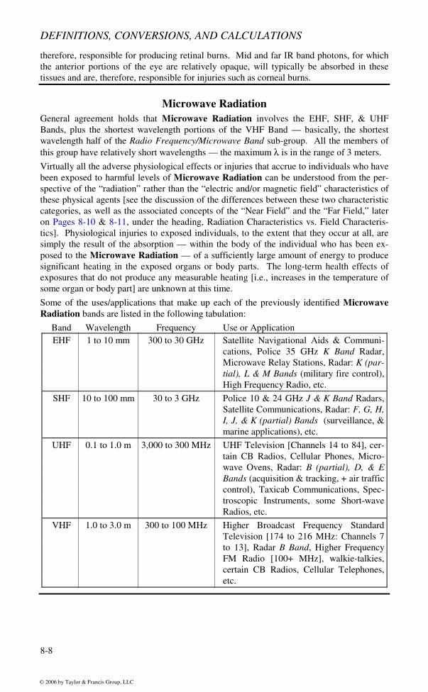
Some of the uses/applications that make up each of the previously identified Microwave Radiation bands are listed in the following tabulation:
Band Wavelength Frequency Use or Application EHF 1 to 10 mm 300 to 30 GHz Satellite Navigational Aids & Communi-
cations, Police 35 GHz K Band Radar, Microwave Relay Stations, Radar: K (par-tial), L & M Bands (military fire control), High Frequency Radio, etc.
SHF 10 to 100 mm 30 to 3 GHz Police 10 & 24 GHz J & K Band Radars, Satellite Communications, Radar: F, G, H, I, J, & K (partial) Bands (surveillance, & marine applications), etc.
UHF 0.1 to 1.0 m 3,000 to 300 MHz UHF Television [Channels 14 to 84], cer-tain CB Radios, Cellular Phones, Micro-wave Ovens, Radar: B (partial), D, & E Bands (acquisition & tracking, + air traffic control), Taxicab Communications, Spec-troscopic Instruments, some Short-wave Radios, etc.
VHF 1.0 to 3.0 m 300 to 100 MHz Higher Broadcast Frequency Standard Television [174 to 216 MHz: Channels 7 to 13], Radar B Band, Higher Frequency FM Radio [100+ MHz], walkie-talkies, certain CB Radios, Cellular Telephones, etc.
Radio Frequency Radiation makes up the balance of the Radio Frequency/Microwave Band sub-group. The specific segments involved are the longest wavelength half of the VHF Band, plus all of the HF, MF, & LF Bands. In general, all of the wavelengths in-volved in this sub-group are considered to be long to very long, with the shortest λ being 3+ meters and the longest, approximately 10 km, or just less than 6.25 miles.
The adverse physiological effects or injuries, if any, that result from exposures to Radio Frequency Radiation can be understood from the perspective of the “electric and/or mag-netic field,” rather than the “radiation” characteristics of these particular physical agents [again, see the discussion of the differences between these two characteristic categories, as well as the associated concepts of the “Near Field” and the “Far Field,” later on Pages 8-10 & 8-11, under the heading, Radiation Characteristics vs. Field Characteristics]. Injuries to exposed individuals, to the extent that they have been documented at all, are also the result of the absorption by some specific organ or body part of a sufficiently large amount of en-ergy to produce highly localized heating. As was the case with Microwave Radiation expo-sures, the long-term health effects of exposure events that do not produce any measurable heating are unknown at this time.
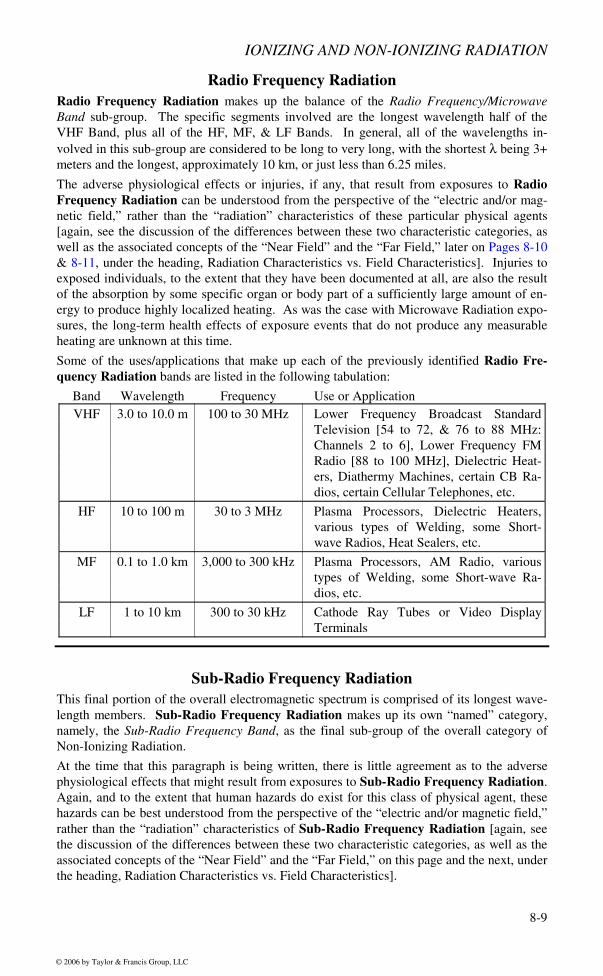
Some of the uses/applications that make up each of the previously identified Radio Fre-quency Radiation bands are listed in the following tabulation:
Band Wavelength Frequency Use or Application VHF 3.0 to 10.0 m 100 to 30 MHz Lower Frequency Broadcast Standard
Television [54 to 72, & 76 to 88 MHz: Channels 2 to 6], Lower Frequency FM Radio [88 to 100 MHz], Dielectric Heat-ers, Diathermy Machines, certain CB Ra-dios, certain Cellular Telephones, etc.
HF 10 to 100 m 30 to 3 MHz Plasma Processors, Dielectric Heaters, various types of Welding, some Short-wave Radios, Heat Sealers, etc.
MF 0.1 to 1.0 km 3,000 to 300 kHz Plasma Processors, AM Radio, various types of Welding, some Short-wave Ra-dios, etc.
LF 1 to 10 km 300 to 30 kHz Cathode Ray Tubes or Video Display Terminals
Sub-Radio Frequency Radiation
This final portion of the overall electromagnetic spectrum is comprised of its longest wave-length members. Sub-Radio Frequency Radiation makes up its own “named” category, namely, the Sub-Radio Frequency Band, as the final sub-group of the overall category of Non-Ionizing Radiation.
At the time that this paragraph is being written, there is little agreement as to the adverse physiological effects that might result from exposures to Sub-Radio Frequency Radiation. Again, and to the extent that human hazards do exist for this class of physical agent, these hazards can be best understood from the perspective of the “electric and/or magnetic field,” rather than the “radiation” characteristics of Sub-Radio Frequency Radiation [again, see the discussion of the differences between these two characteristic categories, as well as the associated concepts of the “Near Field” and the “Far Field,” on this page and the next, under the heading, Radiation Characteristics vs. Field Characteristics].
Primary concern in this area seems generally to be related to the strength of either or both the electric and the magnetic fields that are produced by sources of this class of radiation. The American Conference of Government Industrial Hygienists [ACGIH] has published the following expressions that can be used to calculate the appropriate 8-hour TLV-TWA — each as a function of the frequency, f, of the Sub-Radio Frequency Radiation source be-ing considered. The relationship for electric fields provides a field strength TLV expressed in volts/meter [V/m]; while the relationship for magnetic fields produces a magnetic flux density TLV in milliteslas [mT].
Electric Fields Magnetic Fields
ETLV = 2.5 × 10⁶
f BTLV =
60f
Finally, one area where there does appear to be very considerable, well-founded concern about the hazards produced by Sub-Radio Frequency Radiation is in the area of the ad-verse impacts of the electric and magnetic fields produced by this class of source on the normal operation of cardiac pacemakers. An electric field of 2,500 volts/meter [2.5 kV/m] and/or a magnetic flux density of 1.0 gauss [1.0 G, which is equivalent to 0.1 milliteslas or 0.1 mT] each clearly has the potential for interrupting the normal operation of an exposed cardiac pacemaker, virtually all of which operate at roughly these same frequencies.
Some of the uses/applications that make up each of the previously identified Sub-Radio Frequency Radiation bands are listed in the following tabulation:
Band Wavelength Frequency Use or Application VLF 10 to 100 km 30 to 3 kHz Cathode Ray Tubes or Video Display
Terminals [video flyback frequencies], certain Cellular Telephones, Long-Range Navigational Aids [LORAN], etc.
ULF 0.1 to 1 Mm 3,000 to 300 Hz Induction Heaters, etc.
SLF 1 to 10 Mm 300 to 30 Hz Standard Electrical Power [60 Hz], Home Appliances, Underwater Submarine Communications, etc.
ELF 10 to 100 Mm 30 to 3 Hz Underwater Submarine Communications, etc.
Radiation Characteristics vs. Field Characteristics
All of the previous discussions have been focused on the various categories and sub-categories of the electromagnetic spectrum [excluding, in general, the category of particu-late nuclear radiation]. It must be noted that every band of electromagnetic radiation — from the extremely high frequencies of Cosmic Rays [frequencies often greater than 3 ×10 21 Hz or 3,000 EHz] to the very low end frequencies characteristic of normal electri-cal power in the United States [i.e., 60 Hz] — will consist of photons of radiation possess-ing both electric and magnetic field characteristics.
That is to say, we are dealing with radiation phenomena that possess field [electric and magnetic] characteristics. The reason for considering these two different aspects or factors is that measuring the “strength” or the “intensity” of any radiating source is a process in which only rarely will both the radiation and the field characteristics be easily quantifiable. The vast majority of measurements in this field will, of necessity, have to be made on only one or the other of these two characteristics. It is the frequency and/or the wavelength being
considered that determines whether the measurements will be made on the radiation or the field characteristics of the source involved.
When the source frequencies are relatively high — i.e., f > 100 MHz [with λ < 3 meters] — it will almost always be easier to treat and measure such sources as simple radiation sources. For these monitoring applications [with the exception of situations that involve lasers], it will be safe to assume that the required “strength” and/or “intensity” characteris-tics will behave like and can be treated as if they were radiation phenomena — i.e., they vary according to the inverse square law.
In contrast, when the source frequencies fall into the lower ranges — i.e., f ≤ 100 MHz [with λ ≥ 3 meters] — then it will be the field characteristics that these sources produce [electric and/or magnetic] that will be relatively easy to measure. While it is certainly true that these longer wavelength “photons” do behave according to the inverse square law — since they are, in fact, radiation — their relatively long wavelengths make it very difficult to measure them as radiation phenomena.
These measurement problems relate directly to the concepts of the Near and the Far Field. The Near Field is that region that is close to the source — i.e., no more than a very few wavelengths distant from it. The Far Field is the entire region that exists beyond the Near Field.
Field measurements [i.e., separate electric and/or magnetic field measurements] are usually relatively easy, so long as the measurements are completed in the Near Field. It is in this region where specific, separate, and distinct measurements of either of these two fields can be made. The electric fields that exist in the Near Field are produced by the voltage charac-teristics of the source, while the magnetic fields in this region result from the source’s elec-trical current. Electric field strengths will typically be expressed in one of the following three sets of units: (1) volts/meter — v/m; (2) volts2/meter2 — v2/m2; or (3) milliwatts/cm2 — mW/cm2. Magnetic field intensities will typically be expressed in one of the following four sets of units: (1) amperes/meter — A/m; (2) milliamperes/meter — mA/m; (3) Am-peres2/meter2 — A2/m2; or (4) milliwatts/cm — mW/cm.
Radiation measurements, in contrast, are typically always made in the Far Field. As an example, let us consider a 75,000 volt X-Ray Machine — i.e., one that is producing X-Rays with an energy of 75 keV. For such a machine, the emitted X-Rays will have a frequency of 1.81× 10 19 Hz and a wavelength of 1.66 × 10⁻¹¹ meters, or 0.166 Å [from Planck’s Law]. Clearly for such a source, it would be virtually impossible to make any measurements in the Near Field — i.e., within a very few wavelengths distant from the source — since even a six wavelength distance would be only 1 Å away [a 1 Å distance is less than the diameter of a methane molecule!!]. Measurements made in the Far Field of the strength or intensity of a radiating source then will always be radiation measurements, usually in units such as mil-lirem/hour — mRem/hr. As stated earlier, radiation behaves according to the inverse square law, a relationship that states that radiation intensity decreases as the square of the distance between the point of measurement and the source.
Radioactivity Radioactivity is the process by which certain unstable atomic nuclei undergo a nuclear dis-integration. In this disintegration, the unstable nucleus will typically emit one or more of: (1) the common sub-atomic particles [i.e., the α-Particle, the β-Particles, etc.], and/or (2) photons of electromagnetic energy, [i.e., γ-Rays, etc.].
Radioactive Decay
Radioactive Decay refers to the actual process — involving one or more separate and dis-tinct steps — by which some specific radioactive element, or radionuclide, undergoes the transition from its initial condition, as an “unstable” nucleus, ultimately to a later generation “unstable” radioactive nucleus, or — eventually — a “stable” non-radioactive nucleus. In the process of this Radioactive Decay, the originally unstable nucleus will very frequently experience a change in its basic atomic number. Whenever this happens, its chemical iden-tity will change — i.e., it will become an isotope of a different element. As an example, if an unstable nucleus were to emit an electron [i.e., a β–-particle], its atomic number would increase by one — i.e., an unstable isotope of calcium decays by emitting an electron, and in so doing becomes an isotope of scandium, thus:
20
45 Ca → 21
45Sc + -1
0 e , which could also be written as follows: 2045 Ca → 21
45Sc + β – A second example would be the Radioactive Decay of the only naturally occurring isotope of thorium, which involves the emission of an α-particle:
90232 Th → 88
228Ra + 24 He , which could also be written as follows: 90
232 Th → 88228Ra + 2
4 α In this situation, the unstable thorium isotope was converted into an isotope of radium.
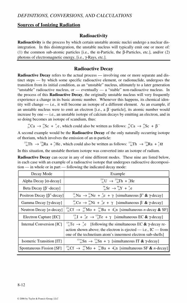
Radioactive Decay can occur in any of nine different modes. These nine are listed below, in each case with an example of a radioactive isotope that undergoes radioactive decomposi-tion — in whole or in part — following the indicated decay mode:
Decay Mode Example
Alpha Decay [α-decay] 92235 U → 90
231Th + 24He
Beta Decay [β–-decay] 3890 Sr → 39
90 Y + -10 e
Positron Decay [β+-decay] 1122 Na → 10
22 Ne + +10e + γ [simultaneous β+ & γ-decay]
Gamma Decay [γ-decay] 2760 Co → 28
60 Ni + –10e + γ [simultaneous β- & γ-decay]
Neutron Decay [n-decay] 98252 Cf → 42
107Mo + 56141Ba + 40
1n [simultaneous n-decay & SF]
Electron Capture [EC] 53125 I + –1
0e → 52125Te + γ [simultaneous EC & γ-decay]
Internal Conversion [IC] 52125 Te → –1
0 e [following the simultaneous EC & γ-decay re-action shown above; the electron is ejected — i.e., IC — from one of the technetium atom’s innermost electron sub-shells]
Radioactive Decay Constant The Radioactive Decay Constant is the isotope specific “time” coefficient that appears in the exponent term of Equation #8-4 on Page 8-18. Equation #8-4 is the widely used rela-tionship that always serves as the basis for determining the quantity [atom count or mass] of any as yet undecayed radioactive isotope. This exponential relationship is used to evaluate remaining quantities at any time interval after a starting determination of an “initial” quan-tity. By definition, all radioactive isotopes decay over time, and the Radioactive Decay Constant is an empirically determined factor that effectively reflects the speed at which the decay process has occurred or is occurring.
Mean Life The Mean Life of any radioactive isotope is simply the average “lifetime” of a single atom of that isotope. Quantitatively, it is the reciprocal of that nuclide’s Radioactive Decay Con-stant — see Equation #8-6, on Page 8-19. Mean Lives can vary over extremely wide ranges of time; as an example of this wide variability, the following are the Mean Lives of two fairly common radioisotopes, namely, the most common naturally occurring isotope of uranium and a fairly common radioactive isotope of beryllium:
For an atom of 92238 U , the Mean Life [α-decay] is 6.44 ×10 9 years
For an atom of 47Be , the Mean Life [EC decay] is 76.88 days
Half-Life
The Half-Life of any radioactive species is the time interval required for the population of that material to be reduced, by radioactive decay, to one half of its initial level. The Half-Lives of different isotopes, like their Mean Lives, can vary over very wide ranges. As an example, for the two radioactive decay schemes described under the definition of Radioac-tive Decay on the previous page, namely, Page 8-12, the Half-Lives are as follows
For 2045 Ca , the Half-Life is 162.7 days
For 90232 Th , the Half-Life is 1.4 × 10¹⁰ years
As can be seen from these two Half-Lives, this parameter can assume values over a very wide range of times. Although the thorium isotope listed above certainly has a very long Half-Life, it is by no means the longest. On the short end of the scale, consider another thorium isotope, 90
218 Th which has a Half-Life of 0.11 microseconds.
Nuclear Fission
Nuclear Fission, as the process that will be described here, differs from the Spontaneous Fission mode that was listed on Page 8-12 under the description of Radioactive Decay as one of the nine radioactive decay modes. This class of Nuclear Fission is a nuclear reac-tion in which a fissile isotope — i.e., an isotope such as 92
235 U or 94239 Pu — upon absorbing a
free neutron undergoes a fracture which results in the conversion of the initial isotope into: 1. two daughter isotopes, 2. two or more additional neutrons, 3. several very energetic γ-rays, and 4. considerable additional energy, usually appearing in the form of heat.
Nuclear Fission reactions are the basic energy producing mechanisms used in every nuclear reactor, whether it is used to generate electric power, or to provide the motive force for a nuclear submarine. One of the most important characteristics of this type of reaction is that
by regenerating one or more of the particles [i.e., neutrons] that initiated the process, the reaction can become self-sustaining. Considerable value can be derived from this process if the chain reactions involved can be controlled. In theory, control of these chain reactions occurs in such things as nuclear power stations. An example of an uncontrolled Nuclear Fission reaction would be the detonation of an atomic bomb.
An example of a hypothetically possible Nuclear Fission reaction might be:
92235 U + 0
1n → 44109Ru + 48
123Cd + 3 01n + 3 γs + considerable energy
In this hypothetical fission reaction, the sum of the atomic masses of the two reactants to the left of the arrow is 236.052589 amu, whereas the sum of atomic masses of all the products to the right of this arrow is 234.856015 amu. Clearly there is a mass discrepancy of 1.196574 amu or 1.987 ×10 –24 grams. It is this mass that was converted into the several γ-rays that were created and emitted, as well as the very considerable amount of energy that was liberated. It appears that Albert Einstein was correct: mass and energy are simply dif-ferent forms of the same thing.
Since Nuclear Fission reactions are clearly sources for a considerable amount of ionizing radiation, they are of interest to occupational safety and health professionals.
Radiation Measurements
The Strength or Activity of a Radioactive Source
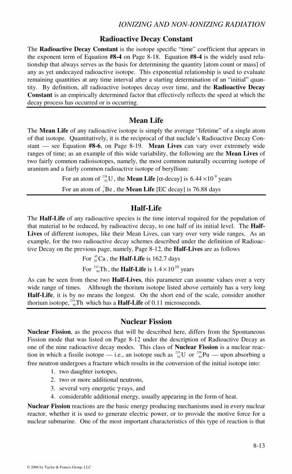
The most common measure of Radiation Source Strength or Activity is the number of radioactive disintegrations that occur in the mass of radioactive material per unit time. There are several basic units that are employed in this area; they are listed below, along with the number of disintegrations per minute that each represents:
Unit of Source Activity Abbreviation Disintegrations/min
1 Curie Ci 2.22 × 10¹²
1 Millicurie mCi 2.22 × 10⁹
1 Microcurie µCi 2.22 × 10⁶
1 Picocurie pCi 2.22
1 Becquerel Bq 60
Exposure Exposure is a unit of measure of radiation that is currently falling into disuse. The basic definition of Exposure — usually designated as X — is that it is the sum number of all the ions, of either positive or negative charge — usually designated as ΣQ — that are produced in a mass of air — which has a total mass, Σm — by some form of ionizing radiation that, in the course of producing these ions, has been totally dissipated. Quantitatively, it is desig-nated by the following formula:
X = Q∑m∑
The unit of Exposure is the roentgen, or R. There is no SI unit for Exposure; thus as stated above this measure is now only rarely encountered. References to Exposure are now only likely to be found in older literature.
Dose, or more precisely Absorbed Dose, is the total energy imparted by some form of ion-izing radiation to a known mass of matter that has been exposed to that radiation. Until the mid 1970s the most widely used unit of Dose was the rad, which has been defined to be equal to 100 ergs of energy absorbed into one gram of matter. Expressed as a mathematical relationship:
1.0 rad = 100 ergs
gram = 100 ergs ⋅ grams –1
At present, under the SI System, a new unit of Dose has come into use. This unit is the gray, which has been defined to be the deposition of 1.0 joule of energy into 1.0 kilogram of mat-ter. Expressed as a mathematical relationship:
1.0 gray = 1.0 joule
kilogram = 1.0 joule ⋅ kilogram –1
The gray is steadily replacing the rad although the latter is still in fairly wide use. For refer-ence, 1 gray = 100 rad [1 Gy = 100 rad], or 1 centigray = 1 rad [1 cGy = 1 rad]. For most applications, Doses will be measured in one of the following “sub-units”: (1) millirad — mrads; (2) microrads — µrads; (3) milligrays — mGys; or (4) micrograys — µGys. These units are — as their prefixes indicate — either 10–3 or 10–6 multiples of the respective basic Dose unit.
Dose, as a measurable quantity, is always represented by the letter “D.”
Dose Equivalent
The Dose Equivalent is the most important measured parameter insofar as the overall sub-ject of radiation protection is concerned. It is basically the product of the Absorbed Dose and an appropriate Quality Factor, a coefficient that is dependent upon the type of ionizing particle involved — see Equation #8-12 on Pages 8-22 & 8-23. This parameter is usually represented by the letter “H.” There are two cases to consider, and they are as follows:
1. If the Dose or Absorbed Dose, D, has been given in units of rads [or mrads, or µrads], then the units of the Dose Equivalent, H, will be rem [or mrem, or µrem] as applicable.
2. If the Dose or Absorbed Dose, D, has been given in units of grays [or mGy, or µGy], then the units of the Dose Equivalent, H, will be sieverts [or mSv, or µSv] as applica-ble.
It is very important to note that since 1 Gray = 100 rads, it follows that 1 sievert = 100 rem.
Finally, if it is determined that a Dose Equivalent > 100 mSv, there is almost certainly a very serious situation with a great potential for human harm; thus, in practice, for Dose Equivalents above this level, the unit of the sievert is rarely, if ever, employed.
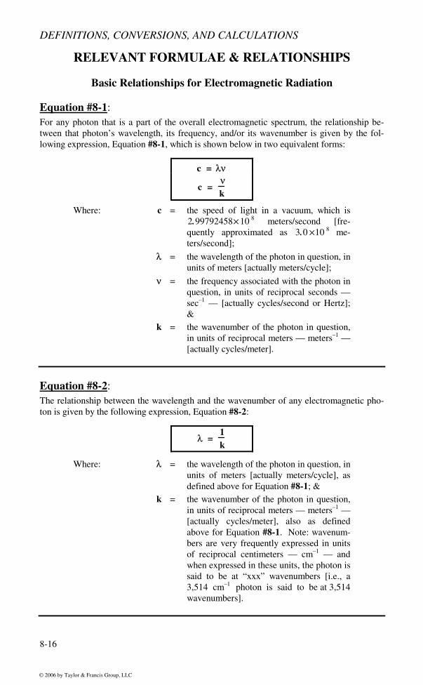
Equation #8-1: For any photon that is a part of the overall electromagnetic spectrum, the relationship be-tween that photon’s wavelength, its frequency, and/or its wavenumber is given by the fol-lowing expression, Equation #8-1, which is shown below in two equivalent forms:
c = λν
c = νk
Where: c = the speed of light in a vacuum, which is 2.99792458× 10 8 meters/second [fre-quently approximated as 3.0 ×10 8 me-ters/second];
λ = the wavelength of the photon in question, in units of meters [actually meters/cycle];
ν = the frequency associated with the photon in question, in units of reciprocal seconds — sec–1 — [actually cycles/second or Hertz]; &
k = the wavenumber of the photon in question, in units of reciprocal meters — meters–1 — [actually cycles/meter].
Equation #8-2: The relationship between the wavelength and the wavenumber of any electromagnetic pho-ton is given by the following expression, Equation #8-2:
λ = 1k
Where: λ = the wavelength of the photon in question, in units of meters [actually meters/cycle], as defined above for Equation #8-1; &
k = the wavenumber of the photon in question, in units of reciprocal meters — meters–1 — [actually cycles/meter], also as defined above for Equation #8-1. Note: wavenum-bers are very frequently expressed in units of reciprocal centimeters — cm–1 — and when expressed in these units, the photon is said to be at “xxx” wavenumbers [i.e., a 3,514 cm–1 photon is said to be at 3,514 wavenumbers].
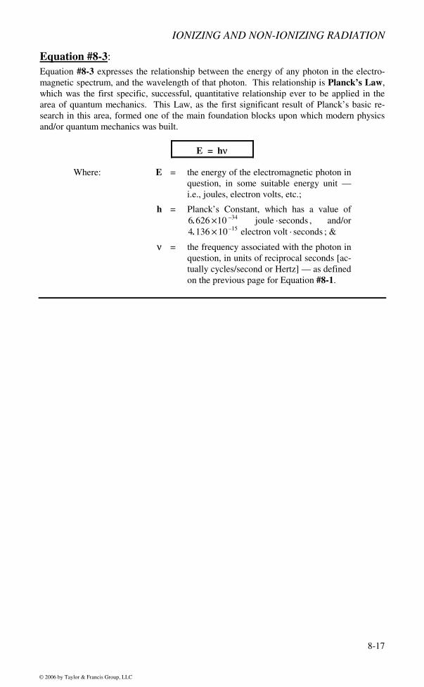
Equation #8-3: Equation #8-3 expresses the relationship between the energy of any photon in the electro-magnetic spectrum, and the wavelength of that photon. This relationship is Planck’s Law, which was the first specific, successful, quantitative relationship ever to be applied in the area of quantum mechanics. This Law, as the first significant result of Planck’s basic re-search in this area, formed one of the main foundation blocks upon which modern physics and/or quantum mechanics was built.
E = hν
Where: E = the energy of the electromagnetic photon in question, in some suitable energy unit — i.e., joules, electron volts, etc.;
h = Planck’s Constant, which has a value of 6.626 ×10 –34 joule ⋅seconds , and/or 4.136 × 10⁻¹⁵ electron volt ⋅ seconds ; &
ν = the frequency associated with the photon in question, in units of reciprocal seconds [ac-tually cycles/second or Hertz] — as defined on the previous page for Equation #8-1.
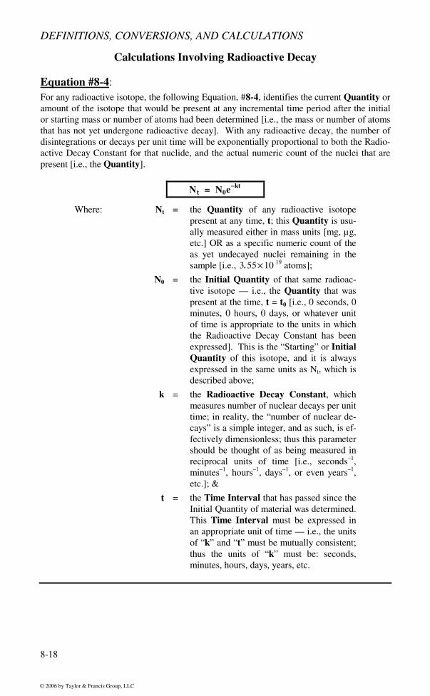
Equation #8-4: For any radioactive isotope, the following Equation, #8-4, identifies the current Quantity or amount of the isotope that would be present at any incremental time period after the initial or starting mass or number of atoms had been determined [i.e., the mass or number of atoms that has not yet undergone radioactive decay]. With any radioactive decay, the number of disintegrations or decays per unit time will be exponentially proportional to both the Radio-active Decay Constant for that nuclide, and the actual numeric count of the nuclei that are present [i.e., the Quantity].
Nt = N0e−kt
Where: Nt = the Quantity of any radioactive isotope present at any time, t; this Quantity is usu-ally measured either in mass units [mg, µg, etc.] OR as a specific numeric count of the as yet undecayed nuclei remaining in the sample [i.e., 3.55× 10 19 atoms];
N0 = the Initial Quantity of that same radioac-tive isotope — i.e., the Quantity that was present at the time, t = t0 [i.e., 0 seconds, 0 minutes, 0 hours, 0 days, or whatever unit of time is appropriate to the units in which the Radioactive Decay Constant has been expressed]. This is the “Starting” or Initial Quantity of this isotope, and it is always expressed in the same units as Nt, which is described above;
k = the Radioactive Decay Constant, which measures number of nuclear decays per unit time; in reality, the “number of nuclear de-cays” is a simple integer, and as such, is ef-fectively dimensionless; thus this parameter should be thought of as being measured in reciprocal units of time [i.e., seconds–1, minutes–1, hours–1, days–1, or even years–1, etc.]; &
t = the Time Interval that has passed since the Initial Quantity of material was determined. This Time Interval must be expressed in an appropriate unit of time — i.e., the units of “k” and “t” must be mutually consistent; thus the units of “k” must be: seconds, minutes, hours, days, years, etc.
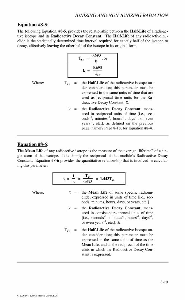
Equation #8-5: The following Equation, #8-5, provides the relationship between the Half-Life of a radioac-tive isotope and its Radioactive Decay Constant. The Half-Life of any radioactive nu-clide is the statistically determined time interval required for exactly half of the isotope to decay, effectively leaving the other half of the isotope in its original form.
T1 2 = 0.693
k, or
k = 0.693T
1 2
Where: T1 2 = the Half-Life of the radioactive isotope un-der consideration; this parameter must be expressed in the same units of time that are used as reciprocal time units for the Ra-dioactive Decay Constant; &
k = the Radioactive Decay Constant, meas-ured in reciprocal units of time [i.e., sec-onds–1, minutes–1, hours–1, days–1, or even years–1, etc.], as defined on the previous page, namely Page 8-18, for Equation #8-4.
Equation #8-6: The Mean Life of any radioactive isotope is the measure of the average ‘lifetime” of a sin-gle atom of that isotope. It is simply the reciprocal of that nuclide’s Radioactive Decay Constant. Equation #8-6 provides the quantitative relationship that is involved in calculat-ing this parameter.
τ = 1k
= T
1 2
0.693 = 1.443T1 2
Where: τ = the Mean Life of some specific radionu-clide, expressed in units of time [i.e., sec-onds, minutes, hours, days, or years, etc.]
k = the Radioactive Decay Constant, meas-ured in consistent reciprocal units of time [i.e., seconds–1, minutes–1, hours–1, days–1, or even years–1, etc.]; &
T1 2 = the Half-Life of the radioactive isotope un-der consideration; this parameter must be expressed in the same units of time as the Mean Life, and as the reciprocal of the time units in which the Radioactive Decay Con-stant is expressed.
Equation #s 8-7 & 8-8: The Activity of any radioisotope is defined to be the number of radioactive disintegrations that occur per unit time. Equation #s 8-7 & 8-8 are two simplified forms of the relationship that can be used to calculate the Activity of any radioactive nuclide.
Equation #8-7:
Ab = kN
Equation #8-8:
⎡ ⎤⎣ ⎦–11
c 10
kNA = = 2.703×10 kN
3.70×10
Where: Ab = the Activity of the radionuclide, expressed in becquerels,
OR
Ac = the Activity of the radionuclide, expressed in curies;
k = the Radioactive Decay Constant, meas-ured in reciprocal units of time [i.e., sec-onds–1, minutes–1, hours–1, days–1, or even years–1, etc.]; &
N = the Quantity of the radioactive isotope that is present in the sample at the time when the evaluation of the Activity is to be made, measured as a specific numeric count of the as yet undecayed nuclei remaining in the sample [i.e., 3.55× 10 19 atoms];
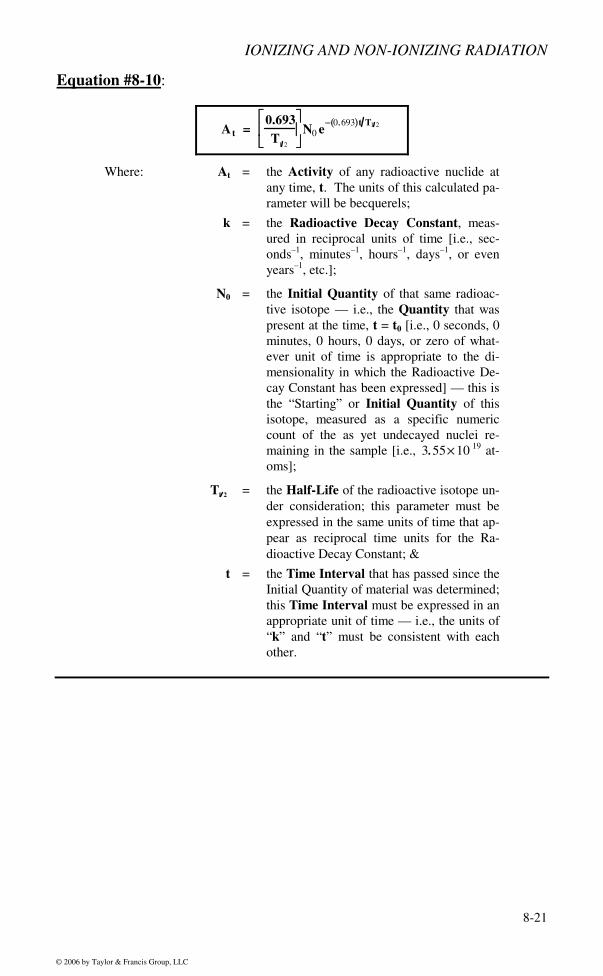
Equation #s 8-9 & 8-10: The following two Equations, #s 8-9 & 8-10, provide the two more general forms of the relationship for determining the Activity of any radioactive nuclide.
Where: At = the Activity of any radioactive nuclide at any time, t. The units of this calculated pa-rameter will be becquerels;
k = the Radioactive Decay Constant, meas-ured in reciprocal units of time [i.e., sec-onds–1, minutes–1, hours–1, days–1, or even years–1, etc.];
N0 = the Initial Quantity of that same radioac-tive isotope — i.e., the Quantity that was present at the time, t = t0 [i.e., 0 seconds, 0 minutes, 0 hours, 0 days, or zero of what-ever unit of time is appropriate to the di-mensionality in which the Radioactive De-cay Constant has been expressed] — this is the “Starting” or Initial Quantity of this isotope, measured as a specific numeric count of the as yet undecayed nuclei re-maining in the sample [i.e., 3.55× 10 19 at-oms];
T1 2 = the Half-Life of the radioactive isotope un-der consideration; this parameter must be expressed in the same units of time that ap-pear as reciprocal time units for the Ra-dioactive Decay Constant; &
t = the Time Interval that has passed since the Initial Quantity of material was determined; this Time Interval must be expressed in an appropriate unit of time — i.e., the units of “k” and “t” must be consistent with each other.
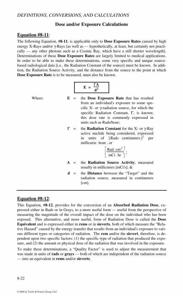
Equation #8-11: The following Equation, #8-11, is applicable only to Dose Exposure Rates caused by high energy X-Rays and/or γ-Rays [as well as — hypothetically, at least, but certainly not practi-cally — any other photons such as a Cosmic Ray, which have a still shorter wavelength]. Determinations of these Dose Exposure Rates are largely limited to medical applications. In order to be able to make these determinations, some very specific and unique source-based radiological data [i.e., the Radiation Constant of the source] must be known. In addi-tion, the Radiation Source Activity, and the distance from the source to the point at which Dose Exposure Rate is to be measured, must also be known.
E = ΓAd2
Where: E = the Dose Exposure Rate that has resulted from an individual's exposure to some spe-cific X- or γ-radiation source, for which the specific Radiation Constant, Γ, is known; this dose rate is commonly expressed in units such as Rads/hour;
Γ = the Radiation Constant for the X- or γ-Ray active nuclide being considered, expressed in units of [Rads ⋅ centimeters ]2 per millicurie ⋅ hour , or
Rad ⋅ cm2
mCi ⋅ hr
⎡
⎣ ⎢
⎤
⎦ ⎥ ;
A = the Radiation Source Activity, measured usually in millicuries [mCi's]; &
d = the Distance between the “Target” and the radiation source, measured in centimeters [cm].
Equation #8-12: This Equation, #8-12, provides for the conversion of an Absorbed Radiation Dose, ex-pressed either in Rads or in Grays, to a more useful form — useful from the perspective of measuring the magnitude of the overall impact of the dose on the individual who has been exposed. This alternative, and more useful, form of Radiation Dose is called the Dose Equivalent and is expressed either in rems or in sieverts, both of which measure the “Rela-tive Hazard” caused by the energy transfer that results from an individual's exposure to vari-ous different types or categories of radiation. The rem and/or the sievert, therefore, is de-pendent upon two specific factors: (1) the specific type of radiation that produced the expo-sure, and (2) the amount or physical dose of the radiation that was involved in the exposure.
To make these determinations, a “Quality Factor” is used to adjust the measurement that was made in units of rads or grays — both of which are independent of the radiation source — into an equivalent in rems and/or sieverts.
This Quality Factor [QF] is a simple multiplier that adjusts for the effective Linear Energy Transfer (LET) that is produced on a target by each type or category of radiation. The higher the LET, the greater will be the damage that can be caused by the type of radiation being considered; thus, this alternative Dose Equivalent measures the overall biological ef-fect, or impact, of an otherwise “simple” measured Radiation Dose.
The “range” of β- and/or α-rays is, as stated earlier, very limited — i.e., the “range” is the distance that any form of radiation is capable of traveling through solid material, such as metal, wood, human tissue, etc. before it is stopped. Because of this, Quality Factors as they apply to alpha and beta particles are only considered from the perspective of internal Dose Equivalent problems. Quality factors for neutrons, X-, and γ-rays apply both to inter-nal and external Dose Equivalent situations.
H Rem = DRad QF[ ] &
HSieverts = DGrays QF[ ]
Where: HRem or HSievert = the adjusted Dose Equivalent in the more useful “effect related” form, meas-ured in either rems or sieverts [SI Units];
DRad or DGray = the Absorbed Radiation Dose, which is independent of the type of radiation, and is measured in either rads or grays [SI Units]; &
QF = the Quality Factor, which is a properly dimensioned coefficient — either in units of rems/rad or sieverts/gray, as applica-ble — that is, itself, a function of the type of radiation being considered [see the following Tabulation].
Tabulation of Quality Factors [QFs] by Radiation Type
Types of Radiation Quality Factors — QFs Internal/External
X-Rays or γ-Rays 1.0 Both β-Rays [positrons or electrons] 1.0 Internal Only Thermal Neutrons 5.0 Both Slow Neutrons 4.0 - 22.0 Both Fast Neutrons 3.0 - 5.0 Both Heavy, Charged Particles [Alphas, etc.] 20.0 Internal Only
Calculations Involving the Reduction of Radiation Intensity Levels
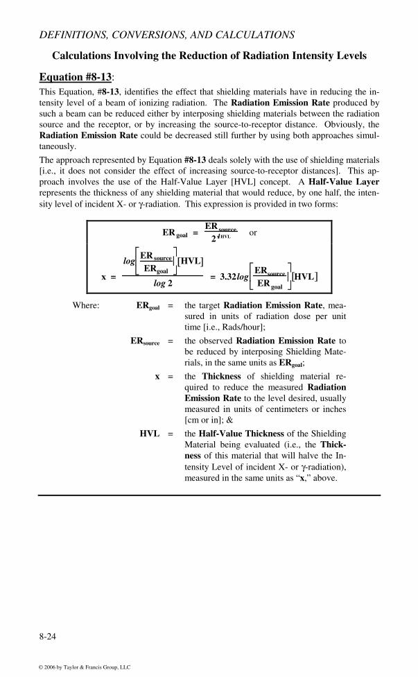
Equation #8-13: This Equation, #8-13, identifies the effect that shielding materials have in reducing the in-tensity level of a beam of ionizing radiation. The Radiation Emission Rate produced by such a beam can be reduced either by interposing shielding materials between the radiation source and the receptor, or by increasing the source-to-receptor distance. Obviously, the Radiation Emission Rate could be decreased still further by using both approaches simul-taneously.
The approach represented by Equation #8-13 deals solely with the use of shielding materials [i.e., it does not consider the effect of increasing source-to-receptor distances]. This ap-proach involves the use of the Half-Value Layer [HVL] concept. A Half-Value Layer represents the thickness of any shielding material that would reduce, by one half, the inten-sity level of incident X- or γ-radiation. This expression is provided in two forms:
ER goal = ER source
2 x HVL or
x =
logER source
ERgoal
⎡
⎣ ⎢
⎤
⎦ ⎥ HVL[ ]
log 2 = 3.32 log
ERsource
ER goal
⎡
⎣ ⎢
⎤
⎦ ⎥ HVL[ ]
Where: ERgoal = the target Radiation Emission Rate, mea-sured in units of radiation dose per unit time [i.e., Rads/hour];
ERsource = the observed Radiation Emission Rate to be reduced by interposing Shielding Mate-rials, in the same units as ERgoal;
x = the Thickness of shielding material re-quired to reduce the measured Radiation Emission Rate to the level desired, usually measured in units of centimeters or inches [cm or in]; &
HVL = the Half-Value Thickness of the Shielding Material being evaluated (i.e., the Thick-ness of this material that will halve the In-tensity Level of incident X- or γ-radiation), measured in the same units as “x,” above.
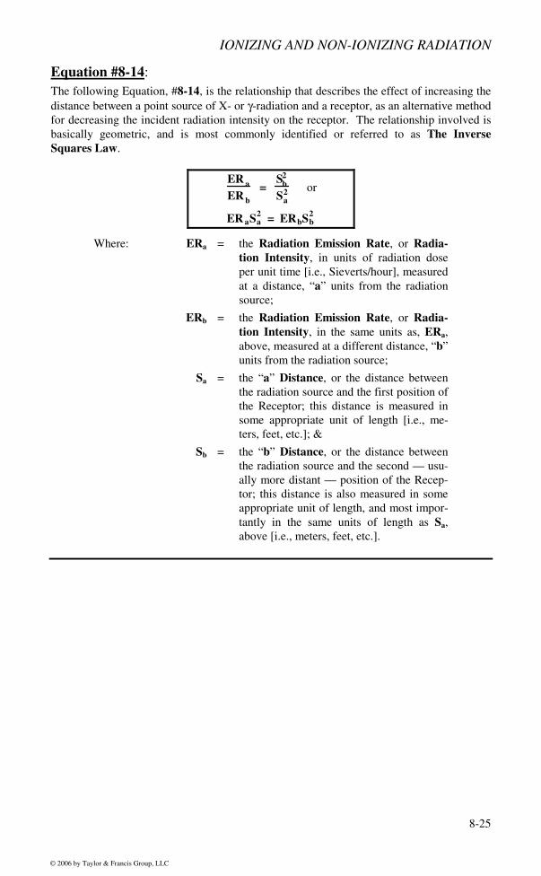
Equation #8-14: The following Equation, #8-14, is the relationship that describes the effect of increasing the distance between a point source of X- or γ-radiation and a receptor, as an alternative method for decreasing the incident radiation intensity on the receptor. The relationship involved is basically geometric, and is most commonly identified or referred to as The Inverse Squares Law.
ER a
ER b =
Sb2
Sa2 or
ER aSa2 = ERbSb
2
Where: ERa = the Radiation Emission Rate, or Radia-tion Intensity, in units of radiation dose per unit time [i.e., Sieverts/hour], measured at a distance, “a” units from the radiation source;
ERb = the Radiation Emission Rate, or Radia-tion Intensity, in the same units as, ERa, above, measured at a different distance, “b” units from the radiation source;
Sa = the “a” Distance, or the distance between the radiation source and the first position of the Receptor; this distance is measured in some appropriate unit of length [i.e., me-ters, feet, etc.]; &
Sb = the “b” Distance, or the distance between the radiation source and the second — usu-ally more distant — position of the Recep-tor; this distance is also measured in some appropriate unit of length, and most impor-tantly in the same units of length as Sa, above [i.e., meters, feet, etc.].
Equation #8-15: The following Equation, #8-15, describes the relationship between the absorption of mono-chromatic visible light [i.e., laser light], and the length of the path this beam of light must follow through some absorbing medium. This formula relies on the fact that each incre-mental thickness of this absorbing medium will absorb the same fraction of the incident ra-diation as will each other identical incremental thickness of this same medium.
The logarithm of the ratio of the Incident Beam Intensity to the Transmitted Beam In-tensity is used to calculate the Optical Density of the medium. This relationship, then, is routinely used to determine the intensity diminishing capabilities [i.e., the Optical Density] of the protective goggles that must be worn by individuals who must operate equipment that makes use of high intensity monochromatic light sources, such as lasers.
OD = logI incident
I transmitted
⎡
⎣ ⎢
⎤
⎦ ⎥
Where: OD = the measured Optical Density of the mate-rial being evaluated, this parameter is di-mensionless;
Iincident = the Incident Laser Beam Intensity, mea-sured in units of power/unit area [i.e., W/cm2]; &
Itransmitted = the Transmitted Laser Beam Intensity, measured in the same units as Iincident, above.
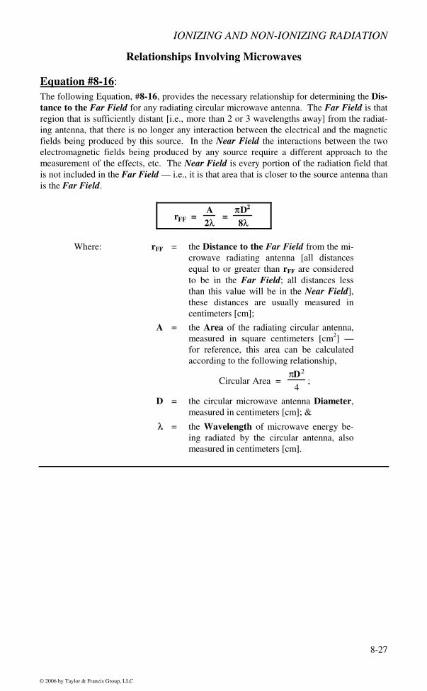
Equation #8-16: The following Equation, #8-16, provides the necessary relationship for determining the Dis-tance to the Far Field for any radiating circular microwave antenna. The Far Field is that region that is sufficiently distant [i.e., more than 2 or 3 wavelengths away] from the radiat-ing antenna, that there is no longer any interaction between the electrical and the magnetic fields being produced by this source. In the Near Field the interactions between the two electromagnetic fields being produced by any source require a different approach to the measurement of the effects, etc. The Near Field is every portion of the radiation field that is not included in the Far Field — i.e., it is that area that is closer to the source antenna than is the Far Field.
rFF = A2λ
= πD2
8λ
Where: rFF = the Distance to the Far Field from the mi-crowave radiating antenna [all distances equal to or greater than rFF are considered to be in the Far Field; all distances less than this value will be in the Near Field], these distances are usually measured in centimeters [cm];
A = the Area of the radiating circular antenna, measured in square centimeters [cm2] — for reference, this area can be calculated according to the following relationship,
Circular Area = πD2
4;
D = the circular microwave antenna Diameter, measured in centimeters [cm]; &
λ = the Wavelength of microwave energy be-ing radiated by the circular antenna, also measured in centimeters [cm].
Equation #8-17: The following Equation, #8-17, provides the relationship for determining the Near Field Microwave Power Density levels that are produced by a circular microwave antenna, radi-ating at a known Average Power Output.
WNF = 4PA
= 16PπD2
Where: WNF = the Near Field Microwave Power Den-sity, measured in milliwatts/cm2 [mW/cm2];
P = the Average Power Output of the mi-crowave radiating antenna, measured in milliwatts [mW];
A = the Area of the radiating circular antenna, measured in square centimeters [cm2] — for reference, this area can be calculated according to the following relationship,
Circular Area = πD2
4; &
D = the circular microwave antenna Diameter, measured in centimeters [cm].
Equations #s 8-18 & 8-19: The following two Equations, #s 8-18 & 8-19, provide the basic approximate relationships that are used for calculating either microwave Power Density Levels in the Far Field [Equation #8-18], OR, alternatively, for determining the actual Far Field Distance from a radiating circular microwave antenna at which one would expect to find some specific Power Density Level [Equation #8-19].
Unlike the Equation at the top of this page [i.e., Equation #8-17], these two formulae have been empirically derived; however, they may both be regarded as sources of reasonably accurate values for the Power Density Levels at points in the Far Field [Equation #8-18], or for various Far Field Distances [Equation #8-19].
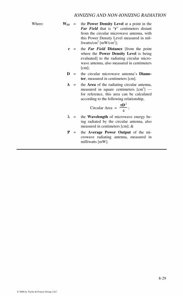
Where: WFF = the Power Density Level at a point in the Far Field that is “r” centimeters distant from the circular microwave antenna, with this Power Density Level measured in mil-liwatts/cm2 [mW/cm2];
r = the Far Field Distance [from the point where the Power Density Level is being evaluated] to the radiating circular micro-wave antenna, also measured in centimeters [cm];
D = the circular microwave antenna’s Diame-ter, measured in centimeters [cm].
A = the Area of the radiating circular antenna, measured in square centimeters [cm2] — for reference, this area can be calculated according to the following relationship,
Circular Area = πD2
4;
λ = the Wavelength of microwave energy be-ing radiated by the circular antenna, also measured in centimeters [cm]; &
P = the Average Power Output of the mi-crowave radiating antenna, measured in milliwatts [mW].
Problem #8.1: The mid-infrared wavelength at which the carbon-hydrogen bond absorbs energy [i.e., the “carbon-hydrogen stretch”] is at approximately 3.35 µ [i.e., 35 microns]. What is the fre-quency of a photon having this wavelength?
Problem #8.2: What is the energy, in electron volts, of one of these “carbon-hydrogen stretch” photons? Remember, the wavelength of these photons is 3.35 µ.
Problem #8.3: What is the wavenumber of the mid-infrared photon that is readily absorbed by a carbon-hydrogen bond [i.e., a photon with a wavelength of 3.35 µ — see Problem #8.1, on the pre-vious page, namely, Page 8-30]?
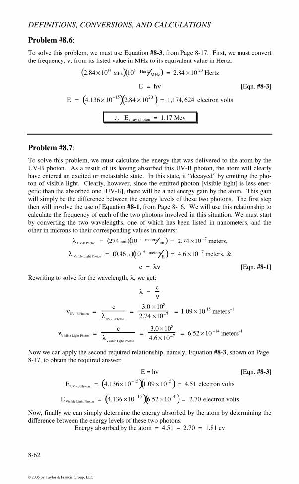
Problem #8.5: What is the wavenumber, in cm–1, of the γ-ray photon identified in Problem #8.4, on the previous page, namely Page 8-31? Remember, this photon has a frequency of 2.84 × 10¹⁴ MHz.
Problem #8.7: An atom is observed, in order: (1) to absorb an ultraviolet [UV-B] photon having a wavelength, λUV-B, of 274 nm, and
then subsequently (2) to emit a visible light photon having a wavelength, λVis, of 0.46 µ.
What was the net energy absorbed by this atom during this process? If the ionization energy of this atom is known to be 1.2 ev, did this process ionize this atom?
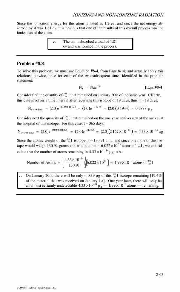
131 I , is frequently used in the treatment of thyroid cancer. It has a Radioactive Decay Constant of 0.0862 days-1. A local hospital received its order of 2.0 µg of this isotope on January 1st. How much of this isotope will remain on January 20th of the same year? How much will remain on the one year anniversary [not a leap anniversary] of the receipt of the 2.0 µg of the 53
Problem #8.10: What would be the measured Activity of the 53
131 I isotope mentioned in Problem #8.8, on Page 8-34, if measurement were made: (1) on January 1st — i.e., the day when it was re-ceived at the Hospital; (2) on January 20th of that same year; and (3) on January 1st of the following year [not a leap year]. Remember, the Radioactive Decay Constant of 53
131 I is 0.0862 days–1, and its mass on January 1st, the day it was received at the Hospital, was 2.0 µg. If it is of any use to you, the atomic weight of the 53
131 I isotope is 130.9061 amu.
Applicable Definitions: Amount of Any Substance Page 1-3
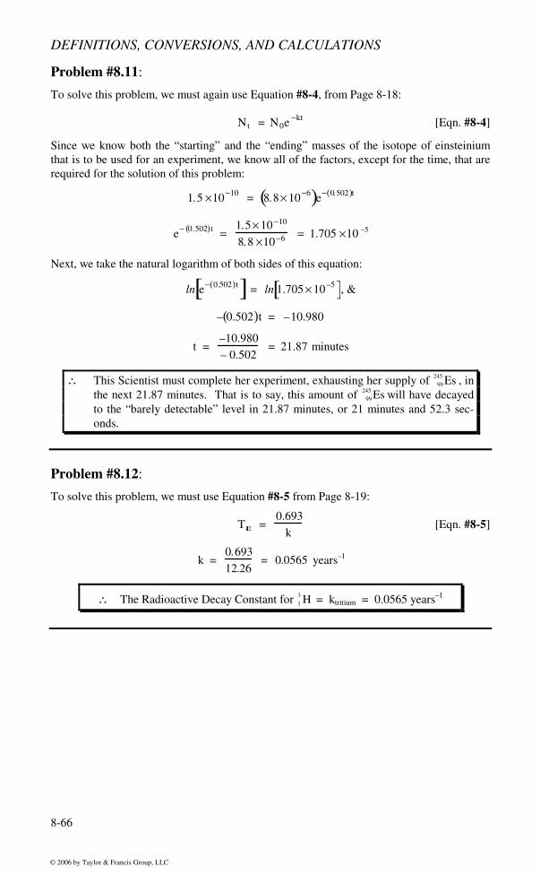
245 Es that can be detected or utilized in any type of experimenta-tion, is 1.5 ×10 –10 ng. The Radioactive Decay Constant for 99
245 Es is 0.502 minutes–1. If 8.8× 10 –6 ng of this material was successfully accumulated by a research scientist, how much time will this scientist have available to her as she performs experiments with her supply of this isotope of einsteinium — i.e., how much time will pass before this quantity has decayed to the “barely detectable” level?
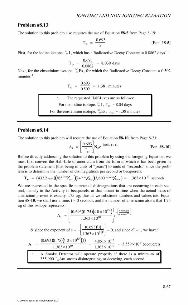
95241 Am is one of the most commonly used and readily available radioactive isotopes. As an example, it is widely used as the ionization source in most commercial smoke detectors. Its Half-Life is 432.2 years. A functional smoke detector must have at least 1.75 µg of this iso-tope in order to operate properly. If there are 4.0 × 10¹⁵ Americium atoms in each micro-gram of this isotope, what is the minimum number of disintegrations per second that are re-quired to operate a smoke detector?
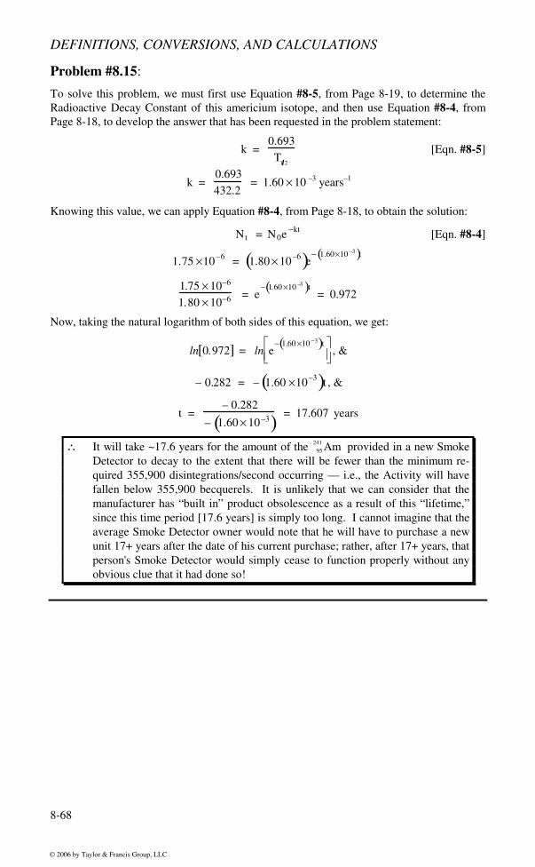
Problem #8.15: If each commercial smoke detector is manufactured with 1.80 µg of 95
241 Am , how long will it be before the minimum required level of radioactive disintegrations per second has been reached — i.e., how long will it take for this isotope’s radioactive decay to reduce the mass of 95
241 Am to 1.75 µg? Is it your opinion that the manufacturer has successfully produced a product with guaranteed obsolescence?
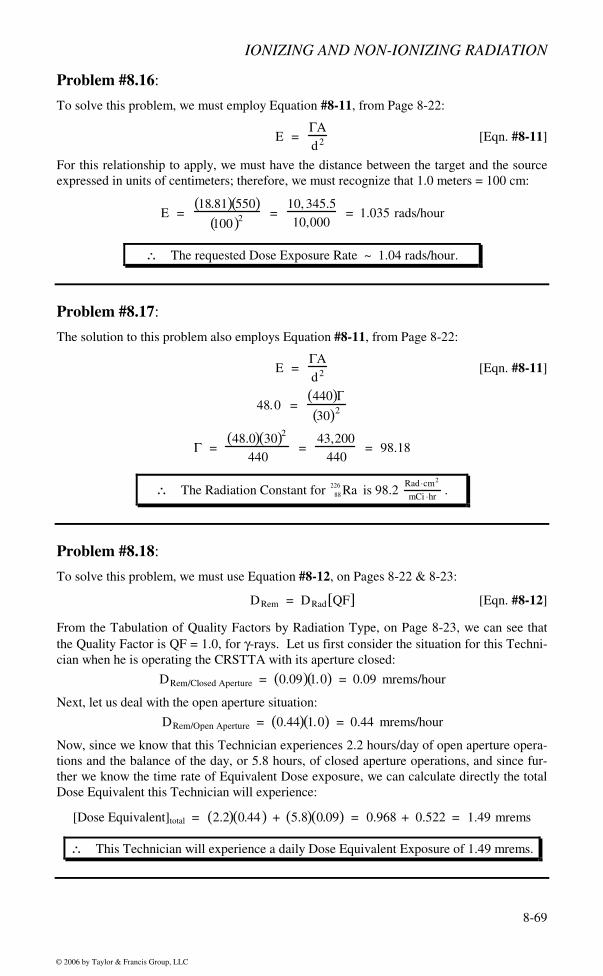
60 Co decays, in part, by emitting relatively high energy γ-rays. It is widely used as a radia-tion source in the treatment of certain cancerous tumors. The Radiation Technician who operates the Cobalt Radiation Source Tumor Treatment Apparatus [the CRSTTA] at a ma-jor hospital accumulates a steady 0.09 mrad, as an absorbed dose, for each hour he is in the room with the CRSTTA when its aperture is closed [i.e., when no patient treatment is oc-curring]. This Technician's absorbed dose increases to 0.44 mrad/hr whenever the CRSTTA's aperture is opened and a patient is being treated — during this treatment period, the Technician occupies a shielded cell in which his radiation exposure is reduced. On a typical day, this facility will have 2.2 hours of open aperture treatment time, and 5.8 hours of closed aperture operations (i.e., set-up, dosimeter development, etc.). What would this Technician's Dose Equivalent be, expressed in rems/day?
Problem #8.19: Among the numerous facilities that it makes available to its staff of Research Scientists — a large research facility has a pool type nuclear reactor, equipped with an externally accessi-ble graphite “Thermal Column.” The Technicians who work 8 hours each day, 5 days each week, around this nuclear reactor accumulate a background absorbed radiation dose at a rate of 0.12 mrads/hour [from thermal, or low energy, neutrons], when the Thermal Column’s access port is closed. Whenever the access port to this Thermal Column is opened — in or-der to work on one of the experiments in it, etc. — each Technician's absorbed dose rate from neutron exposure increases to 0.83 mrads/hour. If this access port is opened only 2 hours each week, and remains closed for the balance of the time, what will be the Dose Equivalent, expressed in an appropriate “sieverts/week” type unit [i.e., mSv/week, µSv/week, etc.], for each of the Technicians who work in this area?
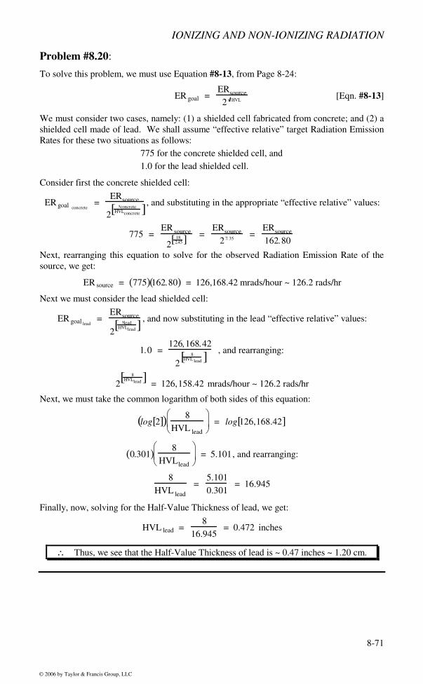
Problem #8.20: The facility described in Problem #8.18, on Page 8-45, was equipped with a new improved shielded cell from which the Radiation Technician could operate the CRSTTA when its aperture was open to provide treatment to a cancer patient. As a result of his operating this facility from his new improved cell, his radiation dose was reduced. The previous cell had been made from concrete, and was 18 inches thick. The improved cell shielding was fabri-cated from lead, and was 8 inches thick. (1) If the Half-Value Thickness for concrete is 2.45 inches; (2) If the radiation emission rate for the 27
60 Co Source in the CRSTTA is 40 rads/hour; (3) If the Technician-to-Source geometry is unchanged [except for the improvements in
the cell shielding]; and (4) If the observed Radiation Emission Rate for this facility has been reduced by a factor
of 775 when the Technician operates the CRSTTA from the new cell; what then would you calculate the Half-Value Thickness of lead to be when used to shield the γ-rays from a 27
Problem #8.21: A patient who has been injected with a quantity of 53
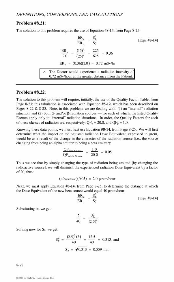
131 I for treatment of his thyroid cancer will, himself, become a radiation source for the γ-radiation emanating from this isotope as it accumulates in his cancerous thyroid gland. A doctor examining this patient from a distance of 15 cm would experience γ-radiation at an intensity of 2 mSv/hour. If this doctor were able to complete his examination at a distance of 25 cm, what would be the Dose Equivalent of radiation he would be experiencing at this increased distance?
Problem #8.22: There is a commercially available therapeutic medical injectant incorporating a low level
88
226 Ra source [an α-emitter]. This material has been compounded so as to accumulate pref-erentially in a patient’s liver. The adjusted radiation dose arising from this product is 40 µrem/hour, when this exposure is measured at a distance of 2.5 mm from the liver. An al-ternative form of this injectant is now also being marketed. This alternative has as its source, the radioisotope, 19
45 K [a β–-emitter]. This alternative injectant has been com-pounded so as to have the same low level of 19
45 K as is the case for the original form contain-ing the 88
226 Ra source. What will be the effect on the adjusted radiation dose that would be experienced at the same 2.5 mm distance from a liver that contains this new injectant? At what distance from such a liver would the adjusted radiation dose be at the same 40 µrem/hour level as was the case for a point 2.5 mm from a liver containing the product with the radium isotope?
Applicable Definitions: Radioactivity Page 8-12
Radioactive Decay Page 8-12
Dose Equivalent Page 8-15
Applicable Formulae: Equation #8-12 Table of “QFs” Page 8-23
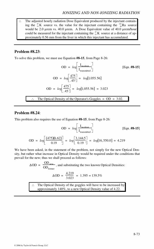
Problem #8.23: The Operator of a laser-based industrial metal trimmer [IR & visible light lasers] wears goggles that reduce the incident beam intensity at his eyes from 475 mW/cm2 [at which level, he would not even be able to see the area he was trimming] to a more workable and safe level of 0.45 mW/cm2, as the transmitted intensity. What is the effective Optical Den-sity of the protective goggles he is wearing?
Problem #8.24: If the industrial metal trimmer identified in Problem #8.23, on the previous page, namely Page 8-51, were to be retrofitted with a new improved laser source that had 6.62 times the laser beam intensity of the original unit, and if it is hoped to reduce still further the transmit-ted beam intensity experienced by the Operator to a new lower level of 0.19 mW/cm2 maxi-mum, by how much must the Optical Density of the goggles be increased to satisfy these new requirements?
Problem #8.25: The UHF Microwave Systems that are used for transmitting a very large fraction of all the public telecommunications in the United States employ a circular antenna with a diameter of 40.5 inches. If these antennas transmit their information using UHF Microwaves that have a wavelength of 46 cm, what will be the distance from these antennas to the Far Field?
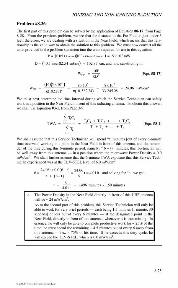
Problem #8.26: If the average power output of the highly focused, very directional UHF Antennas described in Problem #8.25, on the previous page, namely Page 8-53, is 0.05 kilowatts, what will be the approximate Power Density produced by this antenna at a point 12 inches directly in front of it? If the established 6-minute TLV-STEL for this frequency [ν ~ 600 MHz] is 6.0 mW/cm2, for what maximum time period can a Service Technician work, if his assigned task requires that he stand 12 inches away from and directly in front of this transmitting an-tenna? You may assume that his exposure must not exceed the established 6-minute TLV-STEL.
Applicable Definitions: Time Weighted Averages Page 3-2
Microwave Radiation Page 8-8
Radiation vs. Field Characteristics Pages 8-10 & 8-11
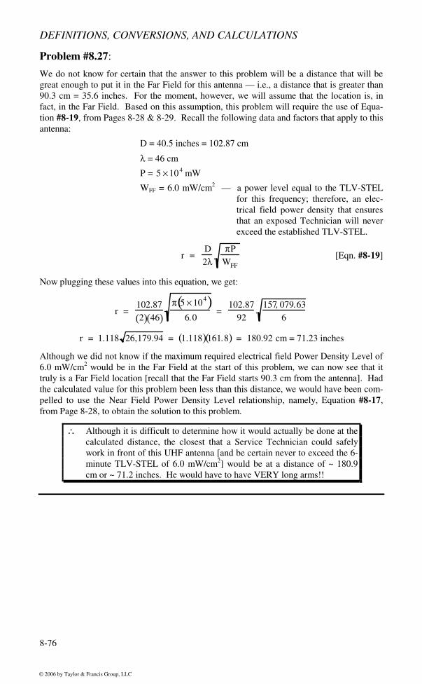
Problem #8.27: In order never to exceed the established TLV-STEL provided in Problem #8.26, on the pre-vious page, namely Page 8-54, what is the closest distance (directly in front of one of these transmitting UHF Antennas) that a Service Technician may safely work for periods of time longer than 6 minutes? Would this position be in the Near or the Far Field for this UHF antenna?
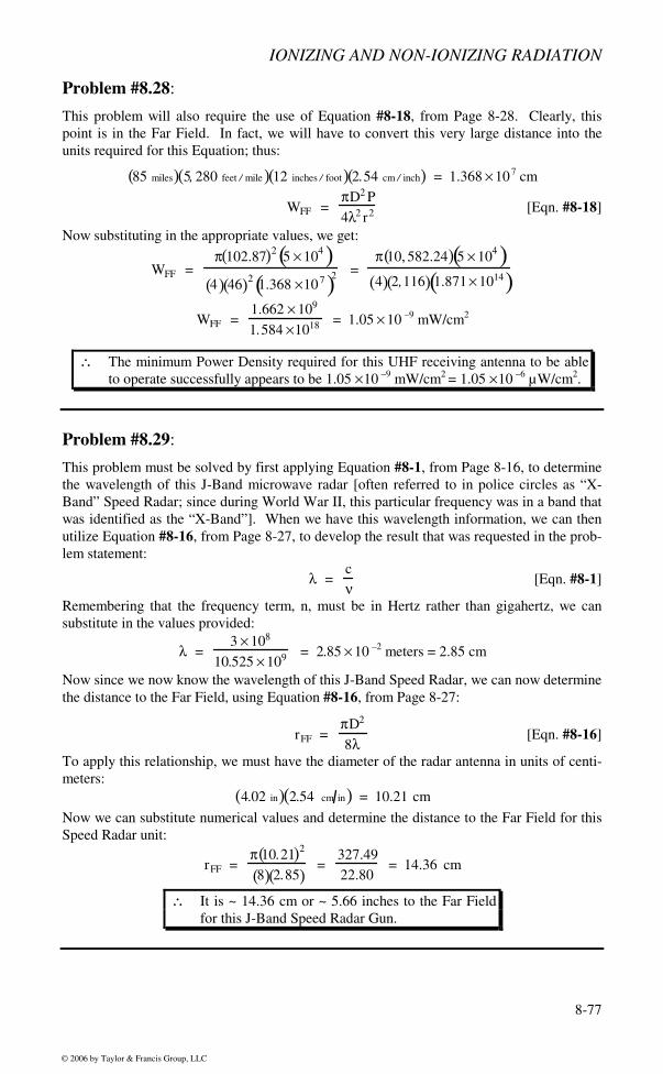
Problem #8.28: If these “line-of-sight” UHF Microwave Antenna Systems can successfully transmit voice or digital data over a distance 85 miles, what is the minimum Power Density Level at which the system's receiving antenna can still be expected to operate successfully?
Problem #8.29: Highway Patrol Officers frequently use a J-Band Radar system to measure the speed of ve-hicles on the highway. These J-Band Speed Radar Guns operate at a microwave frequency of 10.525 GHz, and they radiate from a 4.02-inch diameter antenna. How far is it to the Far Field for such a Radar Gun?
Continuation of Problem Workspace for Problem #8.29
Problem #8.30: The J-Band Speed Radar Gun described in Problem #8.29, on Pages 8-57 & 8-58, has an output power of 45 mW. What is the minimum distance in front of this Gun's antenna that a Highway Patrolman must be in order to ensure that his exposure will never exceed the 6-minute TLV-STEL, which has been established at 10.0 mW/cm2 for this frequency of mi-crowave radar?
SOLUTIONS TO THE IONIZING AND NON-IONIZING RADIATION PROBLEM SET
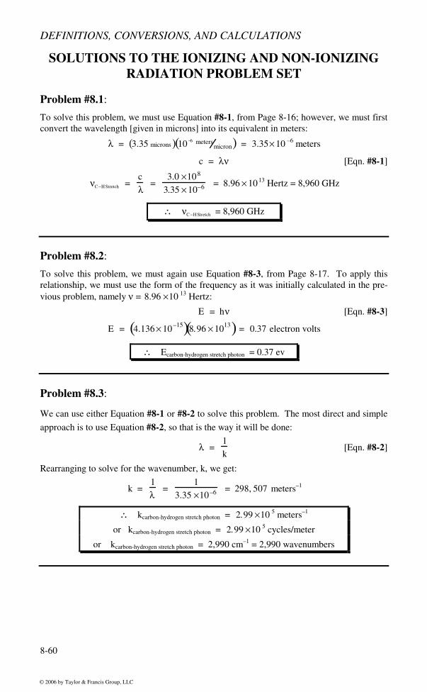
Problem #8.1:
To solve this problem, we must use Equation #8-1, from Page 8-16; however, we must first convert the wavelength [given in microns] into its equivalent in meters:
To solve this problem, we must again use Equation #8-3, from Page 8-17. To apply this relationship, we must use the form of the frequency as it was initially calculated in the pre-vious problem, namely ν = 8.96 ×10 13 Hertz:
E = hν [Eqn. #8-3]
E = 4.136 × 10⁻¹⁵( )8.96 × 10¹³( ) = 0.37 electron volts
∴ Ecarbon-hydrogen stretch photon = 0.37 ev
Problem #8.3:
We can use either Equation #8-1 or #8-2 to solve this problem. The most direct and simple
approach is to use Equation #8-2, so that is the way it will be done:
λ =
1k
[Eqn. #8-2]
Rearranging to solve for the wavenumber, k, we get:
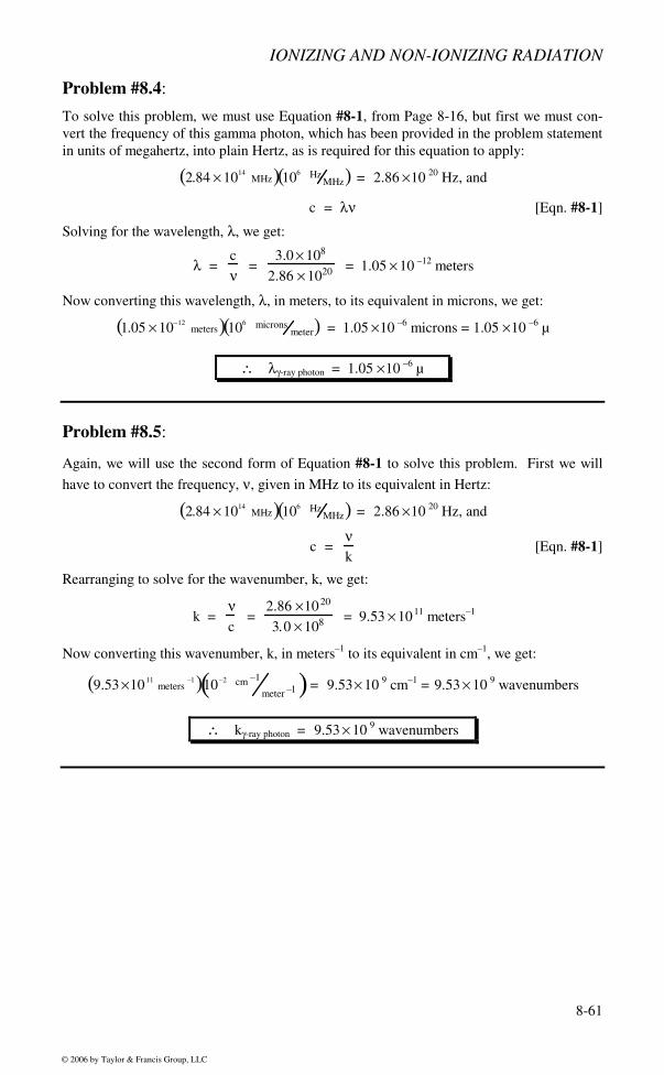
To solve this problem, we must use Equation #8-1, from Page 8-16, but first we must con-vert the frequency of this gamma photon, which has been provided in the problem statement in units of megahertz, into plain Hertz, as is required for this equation to apply:
To solve this problem, we must use Equation #8-3, from Page 8-17. First, we must convert the frequency, ν, from its listed value in MHz to its equivalent value in Hertz:
E = 4.136 × 10⁻¹⁵( )2.84 × 10²⁰( ) = 1,174, 624 electron volts
∴ Eγ-ray photon = 1.17 Mev
Problem #8.7:
To solve this problem, we must calculate the energy that was delivered to the atom by the UV-B photon. As a result of its having absorbed this UV-B photon, the atom will clearly have entered an excited or metastable state. In this state, it “decayed” by emitting the pho-ton of visible light. Clearly, however, since the emitted photon [visible light] is less ener-getic than the absorbed one [UV-B], there will be a net energy gain by the atom. This gain will simply be the difference between the energy levels of these two photons. The first step then will involve the use of Equation #8-1, from Page 8-16. We will use this relationship to calculate the frequency of each of the two photons involved in this situation. We must start by converting the two wavelengths, one of which has been listed in nanometers, and the other in microns to their corresponding values in meters:
Since the ionization energy for this atom is listed as 1.2 ev, and since the net energy ab-sorbed by it was 1.81 ev, it is obvious that one of the results of this overall process was the ionization of the atom.
∴ The atom absorbed a total of 1.81 ev and was ionized in the process.
Problem #8.8:
To solve this problem, we must use Equation #8-4, from Page 8-18, and actually apply this relationship twice, once for each of the two subsequent times identified in the problem statement:
Nt = N0e−kt [Eqn. #8-4]
Consider first the quantity of 53131 I that remained on January 20th of the same year. Clearly,
this date involves a time interval after receiving this isotope of 19 days, thus, t = 19 days:
Since the atomic weight of the 53131 I isotope is ~ 130.91 amu, and since one mole of this iso-
tope would weigh 130.91 grams and would contain 6.022 ×10 23 atoms of 53131 I , we can cal-
culate that the number of atoms remaining in 4.33 ×10 –14 µg to be:
Number of Atoms = 4.33 × 10⁻¹⁴
130.91
⎡
⎣ ⎢
⎤
⎦ ⎥ 6.022 × 10²³[ ] = 1.99 × 10¹⁰ atoms of 53
131 I
∴ On January 20th, there will be only ~ 0.39 µg of this 53131 I isotope remaining [19.4%
of the material that was received on January 1st]. One year later, there will only be an almost certainly undetectable 4.33 ×10 –14 µg — 1.99 × 10¹⁰ atoms — remaining.
To solve this problem we must use, first, Equation #8-5, from Page 8-19, to determine the Half-Life of this isotope. Next we will use Equation #8-6, also from Page 8-19, to deter-mine the Mean Life of an 53
131 I atom. Let us start with the Half-Life determination:
T12 = 0.693
k [Eqn. #8-5]
1 2
0.693T 10.16
0.0682 = = days
Next, let us determine the Mean Life of an 53131 I atom:
τ = 1k
[Eqn. #8-6]
τ = 1
0.0682 = 14.66 days
∴ The Half-Life of the 53131 I isotope = 10.16 days; &
the Mean Life of an 53131 I atom = 14.66 days.
Problem #8.10:
To solve this problem, we will have to employ a large number of relationships. To start with, we will have to determine the actual number of 53
131 I atoms that are present in each of the three time-based scenarios. This atom count is required for the application of either Equation #8-7, from Page 8-20, and/or Equation #8-9, from Page 8-20.
To make these required determinations, we must have specific designations for the three times of interest; thus we shall assign: t0 = 0 days — for the situation on January 1st, the date when the isotope was delivered to the hospital; t19 = 19 days — for the situation on January 20th of that same year; and t365 = 365 days — for the situation one year after the delivery of the isotope to the hospital. We must start this process, for each of the times re-quired, by determining the number of moles of the isotope present at that time. This is done by using Equation #1-10, from Page 1-20:
n = m
MW [Eqn. #1-10]
For the situation on January 1st, when the isotope was delivered to the hospital:
n = 2.0 × 10⁻⁶
130.9061 = 1.53× 10 –8 moles of 53
131 I
Next, we must apply Equation #1-11, from Page 1-20, to determine the atom count on Janu-ary 1st, when the isotope was delivered to the hospital:
n = N
6.022 ×10²³ [Eqn. #1-11]
Transposing this relationship in order to solve for the atom count, Q, we get:
Now, we can address the determination of the required Activity on this date, this time using Equation #8-7, from Page 8-20:
Ab = kN [Eqn. #8-7]
Now, using this relationship, we can determine the Activity level required:
Ab / t = 0 = kNt =0 = 0.0862( ) 9.20 ×10¹⁵( ) = 7.93 × 10¹⁴ becquerels
or, expressed in curies, Ac/t = 0 = 7.93 × 10¹⁴
3.70 × 1010 = 21, 435 curies — a very hot source!!
Next, we can use Equation #8-9, from Page 8-20, to determine the Activities of this source at the other two times of interest:
At = kN0e− kt [Eqn. #8-9]
First, for t = 19 days, we have:
At =19 days = 0.0862( ) 9.20 ×10¹⁵( )e− 0.0862( ) 19( ) = 7.93 × 10¹⁴( )e−1.6378
At =19 days = 7.93 × 10¹⁴( )0.1944( ) = 1.54 × 10 14 becquerels
or again expressing this Activity in curies, we have:
At =19 days = 1.54 × 10¹⁴
3.70 ×1010 = 4,167 curies — still a very hot source!!
Finally, for t = 365 days, we have:
At = 365 days = 0.0862( ) 9.20 ×10¹⁵( )e− 0.0862( ) 365( ) = 7.93 × 10¹⁴( )e−31.463
At = 365 days = 7.93 × 10¹⁴( )2.167 ×10⁻¹⁴( ) = 17.2 becquerels
∴ The three source Activity levels required for the solution of this problem are: At = 0 days = 7.93 × 10 14 becquerels = 21,435 curies At = 19 days = 1.54 × 10¹⁴ becquerels = 4,167 curies
To solve this problem, we must again use Equation #8-4, from Page 8-18:
Nt = N0e −kt [Eqn. #8-4]
Since we know both the “starting” and the “ending” masses of the isotope of einsteinium that is to be used for an experiment, we know all of the factors, except for the time, that are required for the solution of this problem:
1.5 ×10−10 = 8.8× 10⁻⁶( )e− 0.502( )t
e− 0 .502( )t = 1.5× 10⁻¹⁰
8.8 ×10−6 = 1.705 ×10 –5
Next, we take the natural logarithm of both sides of this equation:
ln e− 0.502( )t[ ] = ln 1.705 × 10⁻⁵[ ], &
– 0.502( )t = –10.980
t = –10.980– 0.502
= 21.87 minutes
∴ This Scientist must complete her experiment, exhausting her supply of 99245 Es , in
the next 21.87 minutes. That is to say, this amount of 99245 Es will have decayed
to the “barely detectable” level in 21.87 minutes, or 21 minutes and 52.3 sec-onds.
Problem #8.12:
To solve this problem, we must use Equation #8-5 from Page 8-19:
T12 = 0.693
k [Eqn. #8-5]
k = 0.69312.26
= 0.0565 years–1
∴ The Radioactive Decay Constant for 13 H = ktritium = 0.0565 years–1
The solution to this problem also requires the use of Equation #8-5 from Page 8-19:
T12 = 0.693
k [Eqn. #8-5]
First, for the iodine isotope, 53131 I , which has a Radioactive Decay Constant = 0.0862 days–1:
T12 = 0.6930.0862
= 8.039 days
Next, for the einsteinium isotope, 99245 Es , for which the Radioactive Decay Constant = 0.502
minutes–1:
T12 = 0.6930.502
= 1.381 minutes
∴ The requested Half-Lives are as follows:
For the iodine isotope, 53131 I , T12 ~ 8.04 days
For the einsteinium isotope, 99245 Es , T12 ~ 1.38 minutes
Problem #8.14:
The solution to this problem will require the use of Equation #8-10, from Page 8-21:
At = 0.693
T1 2
⎡
⎣ ⎢
⎤
⎦ ⎥ N0e
− 0.693( )t / T12 [Eqn. #8-10]
Before directly addressing the solution to this problem by using the foregoing Equation, we must first convert the Half-Life of americium from the form in which it has been given in the problem statement [that being in units of “years”] to units of “seconds,” since the prob-lem is to determine the number of disintegrations per second or becquerels:
T12 = 432.2years( ) 365daysyear( )24 hours
day( )3,600 secondshour( ) = 1.363× 10 10 seconds
We are interested in the specific number of disintegrations that are occurring in each sec-ond, namely in the Activity in becquerels, at that instant in time when the actual mass of americium present is exactly 1.75 µg; thus as we substitute numbers and values into Equa-tion #8-10, we shall use a time, t = 0 seconds, and the number of americium atoms that 1.75 µg of this isotope represents:
At = 0.693( )1.75( ) 4.0 × 10¹⁵( )
1.363× 10¹⁰
⎡
⎣ ⎢ ⎢
⎤
⎦ ⎥ ⎥ e
− 0.693( ) 0( )1 .363×10
10⎡ ⎣ ⎢
⎤ ⎦ ⎥
& since the exponent of e = −0.693( )0( )
1.363 ×10¹⁰⎡
⎣ ⎢
⎤
⎦ ⎥ = 0, and since e0 = 1, we have:
At = 0.693( )1.75( ) 4.0 × 10¹⁵( )1( )
1.363× 1010 = 4.851× 10¹⁵
1.363 × 1010 = 3.559 × 10 5 becquerels
∴ A Smoke Detector will operate properly if there is a minimum of 355,900 95
241 Am atoms disintegrating, or decaying, each second.
To solve this problem, we must first use Equation #8-5, from Page 8-19, to determine the Radioactive Decay Constant of this americium isotope, and then use Equation #8-4, from Page 8-18, to develop the answer that has been requested in the problem statement:
k = 0.693T
1 2
[Eqn. #8-5]
k = 0.693432.2
= 1.60 × 10 –3 years–1
Knowing this value, we can apply Equation #8-4, from Page 8-18, to obtain the solution:
Nt = N0e −kt [Eqn. #8-4]
1.75 ×10–6 = 1.80 × 10⁻⁶( )e− 1.60×10 –3( )t
1.75 × 10⁻⁶
1.80 × 10−6 = e− 1.60 ×10 −3( )t
= 0.972
Now, taking the natural logarithm of both sides of this equation, we get:
ln 0.972[ ] = ln e− 1.60 ×10 −3( )t⎡
⎣ ⎢ ⎤ ⎦ ⎥
, &
– 0.282 = – 1.60 ×10⁻³( )t , &
t = – 0.282
– 1.60 × 10⁻³( ) = 17.607 years
∴ It will take ~17.6 years for the amount of the 95241 Am provided in a new Smoke
Detector to decay to the extent that there will be fewer than the minimum re-quired 355,900 disintegrations/second occurring — i.e., the Activity will have fallen below 355,900 becquerels. It is unlikely that we can consider that the manufacturer has “built in” product obsolescence as a result of this “lifetime,” since this time period [17.6 years] is simply too long. I cannot imagine that the average Smoke Detector owner would note that he will have to purchase a new unit 17+ years after the date of his current purchase; rather, after 17+ years, that person's Smoke Detector would simply cease to function properly without any obvious clue that it had done so!
To solve this problem, we must employ Equation #8-11, from Page 8-22:
E = ΓAd2 [Eqn. #8-11]
For this relationship to apply, we must have the distance between the target and the source expressed in units of centimeters; therefore, we must recognize that 1.0 meters = 100 cm:
E = 18.81( ) 550( )
100( )2 = 10, 345.510,000
= 1.035 rads/hour
∴ The requested Dose Exposure Rate ~ 1.04 rads/hour.
Problem #8.17:
The solution to this problem also employs Equation #8-11, from Page 8-22:
E = ΓAd2 [Eqn. #8-11]
48.0 = 440( )Γ30( )2
Γ = 48.0( ) 30( )2
440 =
43,200440
= 98.18
∴ The Radiation Constant for 88226 Ra is 98.2
Rad ⋅cm2
mCi ⋅hr.
Problem #8.18:
To solve this problem, we must use Equation #8-12, on Pages 8-22 & 8-23:
DRem = DRad QF[ ] [Eqn. #8-12]
From the Tabulation of Quality Factors by Radiation Type, on Page 8-23, we can see that the Quality Factor is QF = 1.0, for γ-rays. Let us first consider the situation for this Techni-cian when he is operating the CRSTTA with its aperture closed:
Now, since we know that this Technician experiences 2.2 hours/day of open aperture opera-tions and the balance of the day, or 5.8 hours, of closed aperture operations, and since fur-ther we know the time rate of Equivalent Dose exposure, we can calculate directly the total Dose Equivalent this Technician will experience:
To solve this problem we must first understand the relationship between the units in which each Technician’s Absorbed Dose numbers have been provided, and the units in which the required Dose Equivalent values have been requested in the problem statement. Specifi-cally, remember that, for Absorbed Dose values: 1.0 Gy = 100 rad, and for Dose Equivalent values: 1.0 Sv = 100 rem. In the problem statement we have been given the Absorbed Dose data for each Technician in units of mrads/hour; therefore, it is easy and direct then to con-vert these data into their corresponding Dose Equivalent values in mrems/hour, using Equa-tion #8-12, from Pages 8-22 & 8-23.
Note, too, that we are dealing in an “external” radiation situation — in contrast to an “inter-nal” one, wherein the radiation source is located in some part of a person’s body. We know that Quality Factors for all energy states of neutrons are valid for both internal and external radiation source situations; therefore, we can simply proceed using a QF = 5.0 to develop the solution to this problem.
As stated on the previous page, for thermal neutrons, the Quality Factor = QF = 5.0. We can assume that these Technicians are employed for a 5-day work week, with each workday consisting of 8 hours, thus a 40-hour work week. Let us consider, first, the situation that exists when the Thermal Column’s access port is closed:
HRem = DRad QF[ ] [Eqn. #8-12]
Hrem -closed = 0.12( ) 5.0( ) = 0.60 mrem/hr
Let us consider next the situation when this access port is open:
Hrem -open = 0.83( ) 5.0( ) = 4.15 mrem/hr
Next, we can combine these items of specific hourly Dose Equivalent information to the stated weekly time intervals for the two scenarios under which these Technicians routinely work. Consider first the closed port situation, which involves 38 hours per week:
Next, we consider the situation that exists when the access port is open:
Hopen = 4.15mrem hour( ) 2 hours( ) = 8.30 mrem
For the next step, we need only combine these two data items to determine the Dose Equiva-lent, in units of mrem, that each Technician experiences each week:
Hweekly total = 22.80 + 8.30 = 31.10 mrem
And, since we know that 100 mrem = 1 mSv, we can obtain the answer in the form asked for in the problem statement:
To solve this problem, we must use Equation #8-13, from Page 8-24:
ER goal = ERsource
2 x HVL [Eqn. #8-13]
We must consider two cases, namely: (1) a shielded cell fabricated from concrete; and (2) a shielded cell made of lead. We shall assume “effective relative” target Radiation Emission Rates for these two situations as follows:
775 for the concrete shielded cell, and 1.0 for the lead shielded cell.
Consider first the concrete shielded cell:
ER goal concrete =
ERsource
2xconcrete
HVLconcrete[ ], and substituting in the appropriate “effective relative” values:
775 = ER source
2182.45[ ] =
ERsource
2 7. 35 =
ERsource
162.80
Next, rearranging this equation to solve for the observed Radiation Emission Rate of the source, we get:
The solution to this problem requires the use of Equation #8-14, from Page 8-25:
ERa
ER b
= Sb
2
Sa2 [Eqn. #8-14]
ER a
2.0 =
15( )2
25( )2 = 225625
= 0.36
ER a = 0.36( ) 2.0( ) = 0.72 mSv/hr
∴ The Doctor would experience a radiation intensity of 0.72 mSv/hour at the greater distance from the Patient.
Problem #8.22:
The solution to this problem will require, initially, the use of the Quality Factor Table, from Page 8-23; this tabulation is associated with Equation #8-12, which has been described on Pages 8-22 & 8-23. Note, in this problem, we are dealing with: (1) an “internal” radiation situation, and (2) both α- and/or β-radiation sources — for each of which, the listed Quality Factors apply only to “internal” radiation situations. In order, the Quality Factors for each of these classes of radiation are, respectively: QFα = 20.0, and QFβ = 1.0.
Knowing these data points, we must next use Equation #8-14, from Page 8-25. We will first determine what the impact on the adjusted radiation Dose Equivalent, expressed in µrem, would be as a result of the change in the character of the radiation source (i.e., the source changing from being an alpha emitter to being a beta emitter):
QFBeta Source
QFAlpha Source
= 1.020.0
= 0.05
Thus we see that by simply changing the type of radiation being emitted [by changing the radioactive source], we will diminish the experienced radiation Dose Equivalent by a factor of 20, thus:
40µrem/hour( ) 0.05( ) = 2.0 µrem/hour
Next, we must apply Equation #8-14, from Page 8-25, to determine the distance at which the Dose Equivalent of the new beta source would equal 40 µrem/hour:
∴ The adjusted hourly radiation Dose Equivalent produced by the injectant contain-ing the 19
45 K source vs. the value for the injectant containing the 88226 Ra source
would be 2.0 µrem vs. 40.0 µrem. A Dose Equivalent value of 40.0 µrem/hour could be measured for the injectant containing the 19
45 K source at a distance of ap-proximately 0.56 mm from the liver in which this injectant has accumulated.
Problem #8.23:
To solve this problem, we must use Equation #8-15, from Page 8-26:
OD = logIincident
Itransmitted
⎡
⎣ ⎢
⎤
⎦ ⎥ [Eqn. #8-15]
OD = log475
.45⎡ ⎣ ⎢
⎤ ⎦ ⎥ = log 1,055.56[ ]
OD = log475
.45⎡ ⎣ ⎢
⎤ ⎦ ⎥ = log 1,055.56[ ] = 3.023
∴ The Optical Density of the Operator's Goggles = OD = 3.02.
Problem #8.24:
This problem also requires the use of Equation #8-15, from Page 8-26:
OD = logIincident
Itransmitted
⎡
⎣ ⎢
⎤
⎦ ⎥ [Eqn. #8-15]
OD = log475( ) 6.62( )
0.19
⎡ ⎣ ⎢
⎤ ⎦ ⎥ = log
3,144.5
0.19⎡ ⎣ ⎢
⎤ ⎦ ⎥ = log 16, 550.0[ ] = 4.219
We have been asked, in the statement of the problem, not simply for the new Optical Den-sity, but rather what increase in Optical Density would be required under the conditions that prevail for the new; thus we shall proceed as follows:
∆OD = OD new
ODformer
, and substituting the two known Optical Densities:
∆OD = 4.2193.023
= 1.395 = 139.5%
∴ The Optical Density of the goggles will have to be increased by approximately 140%, to a new Optical Density value of 4.22.
This problem requires the use of Equation #8-16, from Page 8-27:
rFF =
πD2
8λ [Eqn. #8-16]
Remembering that since the antenna diameter term, “D,” for this expression must be in units of “centimeters,” rather than “inches,” we must convert the dimension provided in the prob-lem statement from inches into centimeters:
D = 40.5 inches( ) 2.54 cm inch( ) = 102.87 cm, and now substituting in:
rFF = π 102.87( )2
8( ) 46( ) =
33, 245.08368
= 90.34 cm
∴ The Far Field is ~ 90.3 cm ~ 35.6 inches out in front of this UHF antenna.
The first part of this problem can be solved by the application of Equation #8-17, from Page 8-28. From the previous problem, we see that the distance to the Far Field is just under 3 feet; therefore, we are dealing with a situation in the Near Field, which means that this rela-tionship is the valid way to obtain the solution to this problem. We must now convert all the units provided in the problem statement into the units required for use in this equation:
D = 40.5 inches( ) 2.54 cm inch( ) = 102.87 cm, and now substituting in:
WNF = 16PπD2 [Eqn. #8-17]
WNF = 16( ) 5 × 10⁴( )π 102.87( )2 =
8× 10⁵
π 10, 582.24( ) =
8× 10⁵
33, 245.08 = 24.06 mW/cm2
We must next determine the time interval during which the Service Technician can safely work in a position in the Near Field in front of this radiating antenna. To obtain this answer, we shall use Equation #3-1, from Page 3-9:
TWA =
TiCii =1
n
∑
Tii =1
n
∑ =
T1C1 + T2C 2 + . . . + TnCn
T1 + T2 + . . . + Tn
[Eqn. #3-1]
We shall assume that this Service Technician will spend “t” minutes [out of every 6-minute time intervals] working at a point in the Near Field in front of this antenna, and the remain-der of the time during this 6-minute period, namely, “(6 – t)” minutes, this Technician will be well away from this antenna — in a position where the microwave Power Density = 0.0 mW/cm2. We shall further assume that the 6-minute TWA exposure that this Service Tech-nician experienced was at the TLV-STEL level of 6.0 mW/cm2:
( )( )
24.06t 0.0 6 t 24.066 t 4.011t
t 6 t 6
+ −= = =
+ −, and solving for “t,” we get:
t = 6
4.011 = 1.496 minutes ~ 1.50 minutes
∴ The Power Density in the Near Field directly in front of this UHF antenna will be ~ 24 mW/cm2.
As to the second part of this problem, this Service Technician will only be able to work for very brief periods — each being 1.5 minutes [1 minute, 30 seconds] or less out of every 6 minutes — at the designated point in the Near Field, directly in front of this antenna, whenever it is transmitting. In essence, he will only be able to complete productive work for ~ 25% of the time; he must spend the remaining ~ 4.5 minutes out of every 6 away from this antenna — i.e., ~ 75% of his time. If he exceeds this duty cycle, he will exceed the TLV-STEL, which is 6.0 mW/cm2.
We do not know for certain that the answer to this problem will be a distance that will be great enough to put it in the Far Field for this antenna — i.e., a distance that is greater than 90.3 cm = 35.6 inches. For the moment, however, we will assume that the location is, in fact, in the Far Field. Based on this assumption, this problem will require the use of Equa-tion #8-19, from Pages 8-28 & 8-29. Recall the following data and factors that apply to this antenna:
D = 40.5 inches = 102.87 cm
λ = 46 cm
P = 5 × 10⁴ mW
WFF = 6.0 mW/cm2 — a power level equal to the TLV-STEL for this frequency; therefore, an elec-trical field power density that ensures that an exposed Technician will never exceed the established TLV-STEL.
r = D
2λπP
WFF
[Eqn. #8-19]
Now plugging these values into this equation, we get:
r = 102.872( ) 46( )
π 5 × 10⁴( )6.0
= 102.87
92157, 079.63
6
r = 1.118 26,179.94 = 1.118( )161.8( ) = 180.92 cm = 71.23 inches
Although we did not know if the maximum required electrical field Power Density Level of 6.0 mW/cm2 would be in the Far Field at the start of this problem, we can now see that it truly is a Far Field location [recall that the Far Field starts 90.3 cm from the antenna]. Had the calculated value for this problem been less than this distance, we would have been com-pelled to use the Near Field Power Density Level relationship, namely, Equation #8-17, from Page 8-28, to obtain the solution to this problem.
∴ Although it is difficult to determine how it would actually be done at the calculated distance, the closest that a Service Technician could safely work in front of this UHF antenna [and be certain never to exceed the 6-minute TLV-STEL of 6.0 mW/cm2] would be at a distance of ~ 180.9 cm or ~ 71.2 inches. He would have to have VERY long arms!!
This problem will also require the use of Equation #8-18, from Page 8-28. Clearly, this point is in the Far Field. In fact, we will have to convert this very large distance into the units required for this Equation; thus:
∴ The minimum Power Density required for this UHF receiving antenna to be able to operate successfully appears to be 1.05 ×10 –9 mW/cm2 = 1.05 ×10 –6 µW/cm2.
Problem #8.29:
This problem must be solved by first applying Equation #8-1, from Page 8-16, to determine the wavelength of this J-Band microwave radar [often referred to in police circles as “X-Band” Speed Radar; since during World War II, this particular frequency was in a band that was identified as the “X-Band”]. When we have this wavelength information, we can then utilize Equation #8-16, from Page 8-27, to develop the result that was requested in the prob-lem statement:
λ = cν
[Eqn. #8-1]
Remembering that the frequency term, n, must be in Hertz rather than gigahertz, we can substitute in the values provided:
λ = 3 × 10⁸
10.525 × 109 = 2.85 × 10 –2 meters = 2.85 cm
Now since we now know the wavelength of this J-Band Speed Radar, we can now determine the distance to the Far Field, using Equation #8-16, from Page 8-27:
rFF = πD2
8λ [Eqn. #8-16]
To apply this relationship, we must have the diameter of the radar antenna in units of centi-meters:
4.02 in( ) 2.54 cm in( ) = 10.21 cm
Now we can substitute numerical values and determine the distance to the Far Field for this Speed Radar unit:
rFF = π 10.21( )2
8( ) 2.85( ) =
327.4922.80
= 14.36 cm
∴ It is ~ 14.36 cm or ~ 5.66 inches to the Far Field for this J-Band Speed Radar Gun.
This problem will require the use of Equation #8-1, from Page 8-16, to calculate the wave-length of this J-Band Radar. When this value is known, we use Equation #8-18, from Page 8-28, to obtain the solution requested in the problem statement:
λ = cν
[Eqn. #8-1]
Remembering that the frequency term, n, must be in Hertz rather than gigahertz, we can substitute in the values provided:
λ = 3 × 10⁸
10.525 × 109 = 2.85 × 10 –2 meters = 2.85 cm
Since we now know the wavelength of this J-Band Speed Radar, we can determine the dis-tance at which the required maximum Power Density level occurs; for this step, as stated above, we will use Equation #8-18, from Page 8-28:
WFF = πD2 P
4λ2 r2 [Eqn. #8-18]
Again, remembering that the diameter of this J-Band radar is 4.02 inches = 10.21 cm, we can substitute in the numeric values that we have. Note, this relationship is most commonly used to calculate the Power Density in the Far Field; however, the distance term, “r,” is a factor in the denominator. Thus we will use this relationship — rearranged — to calculate the distance required in the problem statement:
10.0 = π 10.21( )2 45( )
4( ) 2.85( )2 r 2
r 2 = π 10.21( )2 45( )4( ) 2.85( )2 10.0( )
= 14,739.47
324.9 = 45.37, & taking the square root of both sides:
r = 45.37 = 6.74 cm
∴ The distance — in front of this J-Band Speed Radar Gun’s antenna — at which the Power Density Level will be ≤ 10 mW/cm2 will be ~ 6.74 cm, which is ~ 2.65 inches. For any distance greater than this, there will never be any danger of an individual exceeding the established TLV-STEL of 10 mW/cm2; however, at distances less than this, exposures — especially rela-tively long duration exposures — may well exceed this Standard.