Chapter 9 IONOSPHERIC PHYSICS Section 9.1 F.J. Rich Section 9.2 F.J. Rich Section 9.3 Su. Basu 9.1 STRUCTURE OF THE IONOSPHERE of the layers are shown in Table 9-1. This profile is valid only for midlatitudes. In the equatorial region, the profile 9.1.1 Ionospheric Layers is distorted by the geomagnetic field, and in the polar region, the profile is distorted by ionization by energetic particles, The ionized atmosphere of the earth is composed of a magnetospheric coupling, and other effects. series of overlapping layers. In each layer there is an altitude The D region is present only during daylight hours. The of maximum density, above and below which the ionization altitude of the peak density is normally around 90 km, but density tends to drop off. The total ionization profile with this may decrease considerably to ~ 78 km when the solar the layers indicated is shown in Figure 9-1. Characteristics x-ray flux is enhanced. The E region peak density occurs at a peak altitude of 110km. At sunset, the E Region electron MIDLATITUDE DENSITY PROFILES density drops by a factor of 10 or more in a short period 1000 (tens of minutes) before reaching a nighttime equilibrium 800 NEUTRALS density. At night, the region of low density near 150 km SOLAR MAX 600- between the E region and the F region may have a sharply SOLAR MIN TOPSIDE lower density than shown in Figure 9-1 or the density may 400 be great enough so that there is no depletion region de- pending on geophysical conditions. The F region is a com- NIGHTTIME F2 bination of two somewhat different regions. The F1 region ELECTRONS has an altitude peak near 200 km, but is absent at night. 200 F1 The F2 region has a peak near 300 km during the day and 150 at higher altitudes at night. Shortly after sunset, the absolute DAYTIME density near the peak of the F region often increases due to 100 ELECTRONS plasmatransport processes beforedecreasing to a nighttime 80 value. 60 The Topside Ionosphere is the name given to the rest 101 10 2 1 03 104 105 10 6 10 7 108 of the ionosphere above the F region peak. In a simple DENSITY(cm - 3 ) model of the ionosphere, the density of the topside iono- Figure 9-1. Total ionization profile with ionospheric layers. sphere decreases exponentially with height with somechar- Table 9-1. Layers of daytime midlatitude ionosphere. Layer Altitude(km) Major Component Production Cause D 70-90 km NO+, O2 + Lyman Alpha, x-rays E 95-140 km O2 + , NO + Lyman Beta, Soft x-rays, UV Continuum F1 140-200 km O + , NO + He II, UV Continuum (100-800A) F2 200-400 km O + , N + He II, UV Continuum (100-800A) Topside F > 400 km O + Transport from Below Plasmasphere > 1200 km H+ Transport from Below 9-1
9.1 STRUCTURE OF THE IONOSPHERE of the layers are shown in Table 9-1. This profile is validonly for midlatitudes. In the equatorial region, the profile
9.1.1 Ionospheric Layers is distorted by the geomagnetic field, and in the polar region,the profile is distorted by ionization by energetic particles,
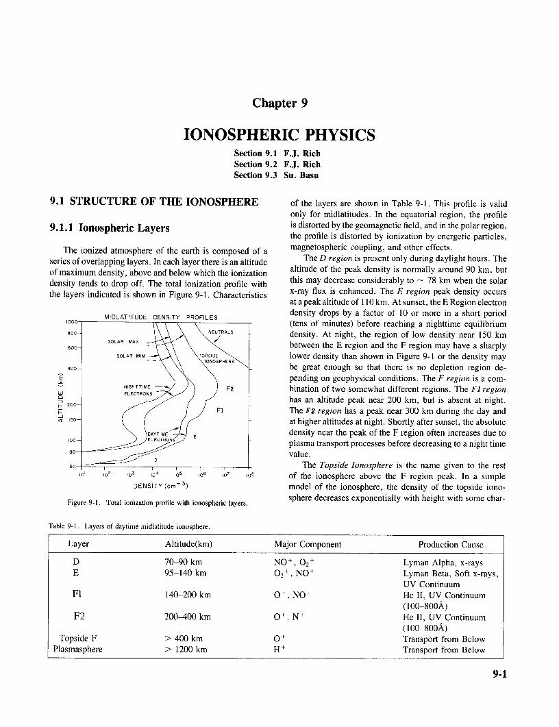
The ionized atmosphere of the earth is composed of a magnetospheric coupling, and other effects.series of overlapping layers. In each layer there is an altitude The D region is present only during daylight hours. Theof maximum density, above and below which the ionization altitude of the peak density is normally around 90 km, butdensity tends to drop off. The total ionization profile with this may decrease considerably to ~ 78 km when the solarthe layers indicated is shown in Figure 9-1. Characteristics x-ray flux is enhanced. The E region peak density occurs
at a peak altitude of 110 km. At sunset, the E Region electronMIDLATITUDE DENSITY PROFILES density drops by a factor of 10 or more in a short period
1000 (tens of minutes) before reaching a nighttime equilibrium800 NEUTRALS density. At night, the region of low density near 150 km
SOLAR MAX600- between the E region and the F region may have a sharply
SOLAR MIN TOPSIDE lower density than shown in Figure 9-1 or the density may400 be great enough so that there is no depletion region de-
pending on geophysical conditions. The F region is a com-NIGHTTIME F2 bination of two somewhat different regions. The F1 region
ELECTRONS has an altitude peak near 200 km, but is absent at night.200
F1 The F2 region has a peak near 300 km during the day and150 at higher altitudes at night. Shortly after sunset, the absolute
DAYTIME density near the peak of the F region often increases due to100 ELECTRONS plasma transport processes before decreasing to a night time80 value.
60 The Topside Ionosphere is the name given to the rest101 10
2 103 104 105 10
610
7 1 0 8 of the ionosphere above the F region peak. In a simpleDENSITY (cm - 3 ) model of the ionosphere, the density of the topside iono-
Figure 9-1. Total ionization profile with ionospheric layers. sphere decreases exponentially with height with some char-
Table 9-1. Layers of daytime midlatitude ionosphere.
Layer Altitude(km) Major Component Production Cause
D 70-90 km NO+, O2 + Lyman Alpha, x-raysE 95-140 km O2+ , NO+ Lyman Beta, Soft x-rays,
UV ContinuumF1 140-200 km O+ , NO+ He II, UV Continuum
(100-800A)F2 200-400 km O +, N+ He II, UV Continuum
(100-800A)Topside F > 400 km O+ Transport from Below
Plasmasphere > 1200 km H+ Transport from Below
9-1
CHAPTER 9
acteristic scale height until the ionization density is below photons v by setting the production rate equal to the lossdetectable levels. In the mid and low latitude ionosphere, rate for a quasi-equilibrium ionosphere. The production ratethe geomagnetic field tends to trap ions, especially hydrogen isions, that would otherwise drift off into deep space. Thus,somewhere between 800 and 2000 km altitude the scale Qv (h) = Bv N(h) Fv (h) ionizations cm -3 s-1 (9.1)height increases to a very large value ( > one earth radius).If one follows a geomagnetic field line out to the equatorial where Bv is the absorption cross section for photoionization,plane and back into the conjugate ionosphere, the density N(h) is the neutral density at the height h, and Fv (h) is thewould change by less than 102 and in some cases less than photon flux of frequency v. The recombination rate is ap-10. This region of trapped ionospheric ions is the Plas- proximatelymasphere [Carpenter and Park, 1973]. The outer edge ofthe plasmasphere where ionospheric ions are not trapped is L, (h) = aR Ni Ne (9.2)the Plasmapause. The plasmapause is located approximatelyalong the geomagnetic field line that maps down to 60° where aR is the recombination coefficient and Ni and Nemagnetic latitude. A representation of the topside iono- are the ion and electron densities. If multiply charged andsphere and plasmasphere is shown in Figure 9-2. negative ions are not important, Ni = Ne. For an appro-
priate set of assumptions, the density near the peak of thelayer is
PLASMA PAUSE DAYSIDE CUSP AURORALLIGHT NORTH
~
Ne(h) ~ 1/2 1- (9.3)PLASMASPHERE 2
where QM is the production at the peak of the layer, hm isthe height of the layer and H is the scale height of the neutral
ANOMALY atmosphere. The parabolic variation of density with h aroundthe peak gives the layers of the ionosphere their character-istic shape.
In principle, the above equation needs to be summedSOUTH over all appropriate frequencies of incident photons to obtain
POLAR CAP the total ionospheric profile. In fact, many details aboutionospheric chemistry (especially in the D and E layers) andabout plasma transport (especially in the F layer) must beconsidered. For example, NO is not a significant component
Figure 9-2. Representation of topside ionosphere and plasmasphere of the neutral atmosphere, but NO+ is a significant ioncomponent due to a chain of chemical reactions induced by
For further information about ionospheric layers see Banks photoionization. Details about computing an ionosphericand Kockarts [1973]; Kohnlein [1978]; and Chapters 12 and model with all factors included is given by Banks and Kock-21. arts [1973].
9.1.2 Chapman Theory for 9.1.3 Ionization Production, LossIonospheric Layers and Vertical Transport
The layering of the ionosphere was first discussed by Ionization production is generally a two-step process.Sydney Chapman in the 1920s. Ionizing photons from the The first step is the creation of ions from the neutrals bysun will produce more and more ions as they penetrate solar photons in the ultraviolet and x-ray spectrum, and todeeper and deeper into an atmosphere with rapidly increas- a lesser degree by collisions with energetic particles. Mosting density. As photoionization occurs, the flux of photons of the ionization is produced by solar radiation with wave-is attenuated until a depth is reached that photoionization lengths less than 1026 A, which ionizes O, O2, and N2.production drops. Thus, a layer of ionization near the al- There are a vast array of minor constituents, especiallytitude of maximum production is created. molecular and metallic ions, that are important in under-
The process of quantitatively determining the height pro- standing the ionosphere. Some of these minor constituentsfile of ionization is outlined as follows. We assume that play important roles in the absorption of solar UV radiationdirect photoionization and recombination are the only sources (especially in the D region), in the production of airglow,of production and loss respectively. We can find the ion in the chemistry of the ionosphere, and in the role of tracersdensity at a height h due to a single frequency of ionizing to indicate ionospheric and atmospheric transport. A review
9-2
IONOSPHERIC PHYSICS
of photoionization is given by Hudson [1971] and Stolarski are important to the dynamics of the ionosphere, especiallyand Johnson [1972]. above the density peak of the F region. Energetic ions can
The second step in the creation of the ionosphere is the undergo a charge exchange process, cross magnetic fieldreaction between ions, neutrals, and electrons to create dif- lines as a neutral and be re-ionized by a second chargeferent forms of ionization than that created by direct ioni- exchange. The result is a transfer of energy across field lineszation. Ionospheric chemistry explains why NO + is an im- that otherwise would be impossible.portant ionospheric ion despite the low abundance of NO The principal loss of ionization comes from recombi-in the neutral atmosphere. Two of the major reactions in nation. This is simply the reaction of positive ions andthe ionosphere which create NO are electrons to form neutrals. The most important recombi-
nation reactions areN2 + O+ -- >NO+ + N
NO+ + e N + ON 2
+ + O ---> NO+ + N (9.4)
O2 + e O + O. (9.6)All of the major reactions are summarized in Figure 9-1 ofTorr [1979]. The reactions that result in minor constituents The charge exchange reactionare quite numerous and not all of them are well understood.Reactions that should be mentioned involve metastable atomic O+ + O2 -- > O2+ + O (9.7)states, negative ions, ionization by photoelectrons, energetic is important to facilitate the recombination process. Theneutrals and vibrational states of molecules. Further details
major problem related to loss of ionization is not a lack ofof ionospheric chemistry are given in Chapter 21.After recombination of ions and electrons to form neu- knowledge of the reactions but a lack of precise knowledge
about the reaction rates. Reaction rates depend upon thetrals, the atoms are often in an excited state that is meta-density of the ions and neutrals, the atomic state of thestable. On the ground, such states are de-excited through incident and resultant ions, the vibrational state of mole-
collisions, but with the lower collision frequency in the cules, and the temperature of the ions and electrons. If onethermosphere, forbidden atomic transitions occur which re-
reaction rate for any related part of the recombination pro-lease photons not generally seen in the laboratory such asthe 5577 A and 6300 A emissions of atomic oxygen. cess is not known precisely, it is difficult to determine the
reaction rate of the complete recombination process. SolarNegative ions are generally found in the D and lower E eclipse data have been used to empirically determine some
regions. They are formed primarily through electron-neutralmolecule collisions. Photodissociation of electrons from of the effective recombination rates. The knowledge of re-
action rates for both production and loss covers a vast arraynegative ions provides the major source of D-region elec-of atomic and molecular reactions [Torr, 1979; Ferguson,trons shortly after sunrise. See Ferguson [1971] and Turco1971; and DNA Rate Rook, 1972] known with varying de-[1974] for a discussion of D-region chemistry. grees of precision
After electrons are removed from an atom by photoion- Vertical transport of ions and electrons is principallyization, they have an energy that depends upon the work
governed by collision frequency and gravity. Below 130function of the atom and the energy of the photon. The km, the collision frequency of ions and electrons is so largeenergy distribution function of photoelectrons is a complex that to a good approximation no ions or electrons enter orfunction [Jasperse, 1977 and Doering et al., 1976] that can leave a unit volume. The unit volume may move up or downcrudely be approximated by a combination of 2 eV and a under the influence of pressure gradients. Between 130 km20 eV Maxwellian distribution. In the D and E regions, the
e e n str n and 300 km the mean free path of electrons, and to a lesserphotoelectrons lose their energy through collisions close to degree ions, becomes comparable or larger than the scalethe location of their formation. In the F region, the photo- height or layer thickness of the ionosphere. Diffusion be-electrons can travel significant vertical distances before los- comes an important factor in plasma transport and energying all of their energy. As a rule of thumb, photoelectrons
exchange. Above an altitude of 300-400 km, the plasmatraveling upward at altitudes above 300 km are consideredcan be treated as collisionless for many purposes. At high
as escaping because of the low collision frequency. Except and midatitudes, vertical transport is approximately alongin the polar regions, these photoelectrons do not truly escape magnetic field lines and particles will tend to diffuse upwardbut follow magnetic field lines into the opposite hemisphere. or downward according to their mass. Becaus e ions andSome of their energy is lost to plasma in the plasmasphere
electrons are electrically coupled, ambipolar diffusion mustand the rest is used to heat and populate the opposite ion-be considered. The ions and electrons diffuse upward to-
osphere [Mantas et al. 19781. Photoelectraons from the op gether at a rate that must be less than a neutral particle withposite hemisphere are most important when one hemisphere the mass of an electron and slightly greater than a neutral
is in darkness and the other in sunlight, particle with the mass of the ion. Near the equator, verticalCharge exchange reactions such as transport is impeded by the magnetic field lines. In the
0* + H - O + H F (9.5) daytime, however, due to electrodynamic effects ionization
9-3
CHAPTER 9
is transported upwards at the magnetic equator which sub- contour of the trough follows the contours of the auroralsequently diffuses down magnetic field lines at + 15 mag- oval instead of paralleling the magnetic latitudes. As thenetic latitudes. This results in the Appleton anomaly as auroral oval moves poleward, the trough moves polewarddiscussed in greater detail in Section 9.2.2.4. and expands in width. As the auroral oval moves equator-
ward, the trough moves equatorward and decreases in width.The depth of the trough (the ratio of minimum density to
9.1.4 Neutral Winds and the density a few degrees equatorward and/or poleward) isHorizontal Transport typically a factor of ten in density or total electron content
(TEC) but may vary from barely discernible to a factor ofBelow 130 km altitude, the ion-neutral collision fre- 103.
quency is so high that ions will freely flow across field lines The equatorward wall of the trough tends to be foundwith the neutrals but the electrons are relatively fixed with on the same field line or 1°-2° poleward of the plasmapause.respect to the magnetic field. As a result, neutral winds tend From this observation has come the suggestion that theto cause ionospheric currents. These ionospheric currents trough is formed by plasma flow upwards into evacuatedare detected on the ground by the diurnal variations in the flux tubes. The region equatorward lies on filled flux tubesmagnetic field at mid and low latitudes (+ 60 to - 60). that can replenish the plasma, and the region poleward ofThe Sq (solar quiet) current system and the equatorial elec- the trough is replenished by ionization induced by precip-trojet are the major current systems related to the neutral itating energetic particles. An alternate explanation is thatwinds. The separation of ions and electrons in the E region the trough is created by the cancellation of the corotationproduce polarization electric fields that can cause E x B and convection electric field in the evening sector. Plasmadrift of plasma in both the E- and F-regions [Evans, 1978]. remains nearly stationery for several hours; depletion is due
Neutral winds are predominantly atmospheric tides with to recombination. After leaving the stagnation zone, theperiods of 24, 12, 8, 6, . . . hours. The zero order neutral trough is sustained through the night by the lack of pro-wind consists of a steady flow away from - 1400 local time duction in the region of the trough.toward ~ 0200. The latitude of these high and low pressure The light ion trough is a sharp drop in H+ and He+zones shifts seasonally with the sun. At high latitudes the density near the peak of F region and in the topside iono-neutral winds are strongly affected by geomagnetic activity sphere. On the night side, the light ion trough or density[Roble et al., 1981]. The ring current, which causes the gradient is collocated with the equatorward wall of the totalnegative Dst midlatitude deflection is dissipated in the ion- ion trough. On the dayside, the light ion trough continuesosphere near 60 which, in turn, heats the thermosphere. to be found near 60° magnetic latitude while the total ionThe Joule heating of the auroral zones and polar caps and trough either ceases to exist or moves to higher latitudes.the heating from precipitating particles also cause the high For a satellite traveling in the altitude range from -800 tolatitude thermosphere to be heated. As a result of the heating - 1500 km on the dayside and -600 to - 1500 km on theof the thermosphere, the neutral winds at high and mid- night side, the light ion trough is seen as a rapid transitionlatitudes can be strongly affected and even reverse direction. between H + and O + as the dominant ion [Titheridge, 1976].
The convection electric fields imposed upon the high Above -1500 km, the O+ density is so low even when itlatitude ionosphere from the magnetosphere also cause hor- is the dominant ion that the total density drops by a factorizontal plasma transport. In the winter ionosphere, the drifts of ~10 to >10 3 at all local times at the same latitude asdriven by the convection electric field are a major source the light ion trough.of ionization in the polar cap drawing from the auroral zone The plasma temperature in the F region near the troughand the dayside [Sojka et al., 1981]. The convection electric and the equatorward wall of the auroral zone is increasedfield can also decrease ionization by enhancing the recom- substantially from the temperature in adjacent regions. Thisbination rates as ions are driven through the neutrals. is partly related to energy from the ring current in the equa-
torial plane of the magnetosphere being transferred to theionosphere. When this energy deposition is large enough,
9.2 HIGH LATITUDE PHENOMENA the airglow is enhanced to form stable auroral red (SAR)arcs. SAR arcs are generally subvisual. They tend to bemost intense following a major geomagnetic storm.
9.2.1 Total Ionization Trough and Light IonTrough.
9.2.2 The Ionosphere in the Auroral Oval.The total ionization trough is a region of decreased F-
region ionization and/or total electron content found in a We have known of the visual displays called auroras forlatitudinally narrow band near 60°-65° magnetic latitude centuries and we have known for the past century that au-[Ahmed et al., 1979]. The ends of the trough are typically roras are associated with electromagnetic disturbances.found an hour after sunset and an hour before sunrise. The However, it has only been since the start of the space age
9-4
IONOSPHERIC PHYSICS
we have known auroras are global and are the projection of An important feature of the high latitude ionosphere isactivity at great altitudes in the magnetosphere and solar that the plasma density is irregular on the scale of meterswind (Chapters 3 and 8). The global nature of auroras is to kilometers vertically and on the scale of meters to hundredgenerally acknowledged by referring to the auroral oval, a of kilometers horizontally. The small scale irregularitiesband a few degrees in latitude and around both magnetic cause scintillation of radio signals passing through the ion-poles where auroral phenomena are found [Feldstein and osphere. The large scale irregularities or density gradientsStarkov, 1967; Meng, 1977; Gussenhoven et al., 1981 and provide a necessary condition for various plasma turbulence1983; see also Chapter 12]. The optical emissions are a mechanisms that result in small scale irregularities (see Chapterresult of the energy from precipitating energetic particles 10). The causes of irregularities in the auroral zone are(mostly electrons) being deposited in the ionosphere. Op- numerous [Fejer and Kelley, 1980] but are related to factorstical emissions visible to the naked eye are mostly in narrow such as particle precipitation and E x B drifts. The regionlatitudinal bands (1 to 10 km in width) called auroral arcs, of auroral zone scintillations extends equatorward of thebut there are precipitating particles and optical emissions optical auroral [Martin and Aarons, 1977], but are roughlythroughout the auroral zone. In the equatorward portion of collocated with the region of particle precipitation. Somethe auroral oval the optical emissions are spatially uniform of the strongest scintillations are observed when the ray pathand are known as the diffuse aurora. Along the poleward of the radio signal is aligned with the magnetic L-shell inportion of the oval, the precipitating particles tend to be the F region. This has been analyzed to indicate that irreg-grouped into bands about 1° wide. The intensity and max- ularities are in the form of sheets extended along the mag-imum energy of the precipitating particles are greatest in netic field and in the magnetic E-W direction [Rino et al.,the center of the band and fall off near the edges of the 1978].band. These have been called "inverted-V" events due totheir signature in the records of polar orbiting satellites. Ifthe maximum intensity is great enough, a visible auroralarc will appear at the center of the inverted-V event.
The precipitating energetic particles lose energy to the In the ionosphere, a substorm is an intensification ofprocesses and structures that are normally observed in theatmosphere by ionizing neutrals in a manner similar to the
ionization caused by protons. If the precipitating particles quiet time auroral zone ionosphere. See Chapter 8 for aall had the same energy, a thin layer of ionization would complete description. During a substorm the flux and av-be formed. The altitude of the ionization layer is determined erage energy of the precipitating particles increase rapidlyfrom the energy of the precipitating particles: 10 keV elec- and substantially. This causes more visible features to ap-trons produce an ionization layer near 110 km altitude; 500 pear. The increase in the energy of the particle causes ion-eV electrons produce an ionization layer near 180 km al- ization in the lower E layer that is not present during quiettitude. The density of the ionization layer is determined by times. The increased activity causes an increase in the scin-the intensity of the particle flux. tillation producing irregularities. The increased E x B drift
In the nighttime auroral zone, the electron density profile rates heat the ionosphere and increase the scale heights.During the early phases of a substorm, the auroral zone
can be accurately estimated if the spectrum of precipitating moves equatorward several degrees in 10-20 minutes. Theparticles is known, or conversely the spectrum of precipi-tating particles can be estimated from the electron density trough either moves equatorward with the auroral zone
movement or ceases to exist during the substorm dependingprofile [Vondrak and Baron, 1977]. This is especially truein the E region where the ionization lifetimes are short. In on geomagnetic conditions and local time. During the late
phases of a substorm the auroral oval contracts polewardthe F region where ionization lifetimes are long, the ioni-zation present at any given moment is influenced by the and precipitationprecipitation over the past few minutes to tens of minutesas well as the instantaneous precipitation. Also, vertical andhorizontal transport has a major effect upon the structure of 9.2.4 Polar Cap Structure.the F region. Regions of enhanced F region ionization candrift many degrees from the production region [Vickrey et The polar cap ionosphere is relatively placid comparedal., 19801. to the auroral zone, but soft particle precipitation known as
In the sunlit auroral zone, photoionization dominates the polar rain [Winningham and Heikkila, 19741 does affect theproduction of ionization, but ionization from particles has polar cap ionosphere. In the summer months, the polar capa major effect on plasma irregularities. Also, in limited ionosphere is dominated by photoionization similar to thealtitude regions the ionization from particles can occasion- midlatitude ionosphere. In the winter months, ionization isally dominate photoionization. Even where the photoioni- generally maintained by the polar rain and by convectionzation is the dominant source, the heat from precipitating from the day side to the night side of the polar cap. In theparticles increases the scale height of the ionosphere and winter months, the F layer can be sunlit while the E layerthe neutrals. is in darkness. This can lead to He+ being the dominant
9-5
CHAPTER 9
ion in parts of the topside ionosphere. During times of weak where n is the electron or ion concentration, e is the elec-convection and precipitation, the winter polar ionosphere tronic charge, ve and vi are the electron and ion collision fre-near the midnight sector can decay to very low levels of quencies, and me and mi are the masses of an electron and anionization; this area is called the polar hole [Brinton et al., ion respectively. The longitudinal conductivity is indepen-1978]. dent of magnetic field intensity and is identical to the con-
Since the magnetic field lines in the polar cap diverge ductivity obtained in the absence of any magnetic field.effectively toward infinity, the H+ in the polar ionosphere When an electric field is applied perpendicular to theescapes rapidly in a process known as the polar wind. Unlike magnetic field, the conductivity in the direction of the elec-the midlatitude ionosphere, O+ is generally the dominant tric field is called the Pedersen conductivity and is given byion at all altitudes of the F-region.
1 = ne2 +
9.3 EQUATORIAL PHENOMENA ) ((9.9)
9.3.1 Sq Current System where e and i are the electron and ion gyrofrequenciesrespectively.
See Chapter 4. In such cases of a crossed electric and magnetic field,a Hall current usually flows perpendicular to both the electricand magnetic fields and the resulting conductivity, called
9.3.2 Equatorial Electrojet the Hall conductivity, is given by
The intense eastward ionospheric current that flows byday over a narrow latitudinal strip along the magnetic equa- 2 i
tor is known as the equatorial electrojet [Matsushita and 2 = ne2 +Campbell, 1967]. The electrojet causes the large daily vari-me (ve2 +e2 mi(vi2 +i2)ations of the horizontal component of magnetic field inten- (9. 10)sity recorded by ground magnetometers near the magneticequator. The ionospheric current system is a result of a At the magnetic equator, an eastward electric field isdynamo action of the horizontal wind system and the elec- developed by the dynamo action of the horizontal windtrical conductivity of the ionosphere in the presence of the system, which gives rise to a motion of charged particleselectrons and ions. The concentration of ionospheric current in the east-west direction (X) due to the Pedersen conduc-near the magnetic equator is a result of the high value of tivity and in the vertical direction (Z) due to the Hallelectrical conductivity of the upper atmosphere at the dip conductivity 2. In view of the horizontal stratification ofequator, which arises from an inhibition of Hall current due the ionosphere, the flow of Hall current in the vertical di-to the horizontal configuration of the earth's magnetic field rection (Z) is totally inhibited and a polarization electricand the horizontal stratification of the ionosphere. field (Ez) develops. In such a case the current densities Jx,
The electrical conductivity of the ionosphere is not only Jz in the X and Z directions can be expressed asgoverned by the concentration of the charged particles butby the neutral particles and the earth's magnetic field as Jx = 1Ex + 2 Ezwell [Chapman, 1956]. Through collisions the neutral par-ticles restrict the motion of charged particles under the action Jz = - 2Ex + 1Ez= 0of any impressed electric field. The presence of the magnetic 2field, on the other hand, restricts the motion of charged or, Jx = + Exparticles across the magnetic field and therefore makes the 2conductivity anisotropic. 2
When a dc electric field is impressed parallel to the or, Jx/Ex = 1 +magnetic field, the longitudinal electrical conductivity that 1
exists parallel to the magnetic field is given by = 3 · (9.11)
The resulting conductivity in the east-west direction is called
ne2 1 (9.8) the Cowling conductivity 3.meve+ mivi, The variations of Pederson 1, Hall 2, and Cowling
3 conductivities with altitude at the magnetic equator are
9-6
IONOSPHERIC PHYSICS
shown in Figure 9-3a for an assumed variation of electron 9.3.3 Electrojet Irregularitiesdensity N and temperature T shown in Figure 9-3b. Theenhanced value of the Cowling conductivity in the dynamo lonosondes first detected the existence of a distinct typeregion is sufficient to account for the intensity of the equa- of sporadic E near the magnetic equator which is patchytorial electrojet. Away from the equator, the geomagnetic and transparent to radio waves reflected from higher layers.
The intensity of equatorial Es (or Esq) is strongly correlated
T, deg with the strength of the electrojet current discussed in the0 0.5 1.0 1.5 x 10³ last section [Matsushita, 1951]. A typical ionogram showing
250 (a) (b) Esq echoes is shown in Figure 9-4. VHF forward scatter
200
150
O2 10 2080
0 5 10 0 1 2 3x10⁵ f(Mc/s)
,emu N, cm-3
(a) (b)Figure 9-4. The typical equatorial sporadic E configuration on an iono-
gram recorded at Huancayo, Peru at 1229 hr (75°W) on 19Figure 9-3. (a) Variation of Pedersen I, Hall 2 , and Cowling 3 con- April 1960 [Cohen et al., 19621.
ductivities with altitude for an ionosphere in which electrondensity N and temperature T vary as shown at (b). Note thatscale for 3 is smaller than I and 2 by a factor of 10[Chapman and Raja Rao, 1965, based on Chapman, 1956]. experiments established that these echoes arise as a result
of scattering from field aligned irregularities of electron
field is no longer horizontal, which allows the Hall field to density immersed in the equatorial electroject [Bowles andleak away. Baker and Martyn [1952] estimated that the half- Cohen, 19621.width of the strip of enhanced east-west conductivity around The important characteristics of the electrojet irregular-the dip equator is about 3° in latitude. The equatorial elec- ities as related to the physics of the scattering region havetrojet corresponds to an east-west electric field of 0.5 mV/m been probed by the VHF radar measurements performed at
and a vertical polarization field of about 10 mV/m. This the Jicamarca Radio Observatory. Radar spectral studiesgives rise to an eastward current or westward electron drift have shown the existence of two classes of irregularitiesof several hundred m/s. The electron drift is westward by called Type 1 and Type 2, associated with the electrojetday and eastward at night. This electrojet model was studied [Balsley and Farley, 1973; Farley and Balsley, 1973; Fejerin detail by Sugiura and Cain [1966]. More complete models and Kelley, 1980].allowing for vertical currents have been discussed by Untiedt Type 1 irregularities have a very narrow spectrum with[1967], Sugiura and Poros [1969], Richmond [1973], and a Doppler shift corresponding approximately to the ionothers. acoustic velocity of about 360 m/s. Farley [1963] and Bune-
The equatorial electrojet current has been observed to man [1963] have explained the Type 1 irregularities byreverse its normal direction during day or night and during showing that a plasma is unstable to waves when the relativemagnetically quiet or disturbed condtions; this reverse cur- electron-ion drift velocity in the direction of the wave ex-rent system has been termed the counter electrojet [Gouin ceeds the ion acoustic velocity. As such, Type 1 irregular-and Mayaud, 1967; Hutton and Oyinloye, 1970; Rastogi, ities are also called two-stream irregularities. Type 2 irreg-1973; Fejer et al., 1976; Fejer and Kelley, 1980]. The rapid ularities on the other hand have phase velocities smaller
reversals during disturbed conditions have been related to than the ion-acoustic velocity and are observed even whenmagnetospheric and high-latitude phenomena [Matsushita the eastward drift velocity is very small during the day.and Balsley, 1972], whereas the reversals during quiet con- Type 2 irregularities are identified with Esq echoes in ion-
ditions have been related to lunar tides [Rastogi, 1974]. ograms and both disappear under counter electrojet condi-
9-7
CHAPTER 9
tions during the daytime. At night the Type 2 irregularities equator and plasma diffusion along geomagnetic field linesare almost always observed except for momentary disap- [Martyn, 1959]. Figure 9-6 illustrates how the eastward E-pearance when the electrojet electric field reverses sign. The region dynamo electric field at locations slightly off theType 2 irregularities are explained by the gradient drift magnetic equator maps to F-region altitude over the equator.instability mechanism. This is because the horizontal po- The eastward electric field in conjunction with the northwardlarization field arising from a relative electron-ion drift inthe electrojet region can, in the presence of the earth'smagnetic field, develop a drift in the direction of the ver-tically oriented density gradient and give rise to these ir-regularities [Fejer and Kelley, 1980].
F F
9.3.4 Equatorial Anomaly and Fountain E E
Effect
During the equinox the sun is overhead at the equator, Figure 9-6. The F region geomagnetic anomaly. Near the equator the
and in terms of solar control the ionization density is ex- electric fields of the atmospheric dynamo in the E layer arepected to be maximum in that region. Instead, the daytime conveyed upwards along geomagnetic lines of force to theionization density at the F2 peak shows a pronounced trough motor in the F layer where they produce an upwards move-
ment of the plasma during the day. The raised plasma thenat the magnetic equator and crests at about 30°N and 30°S diffuses down lines of force to produce enhanced concentra-magnetic dip. This anomalous latitude variation of F 2 ion- tion at places on each side of the equator and decreased
ization near the magnetic equator obtained from bottomside concentration at the equator itself [Ratcliffe, 1972].
ionograms illustrated in Figure 9-5, was first recognized bygeomagnetic field gives rise to a vertically upward plasmamotion. At high altitudes over the equator, the plasma en-counters field lines that connect to the F2 peak at 30°N and30°S magnetic dip along which the plasma diffuses underthe action of gravity. Such plasma transport depletes the F2ionization at the equator and increases the density at loca-tions 30°N and 30°S. Theoretical studies of the equatorialanomaly on a more rigorous basis have been performed by
340 km many workers [see Hanson and Moffett, 1966 and references300 therein].
The transport processes involved in the formation of theO(Nm) equatorial anomaly are best illustrated by the Alouette I
(O) topside sounder results. Figure 9-7 shows the variation ofO ([]) ionization density as a function of height and latitude in the
240 daytime topside ionosphere. At high altitudes over the mag-netic equator, the density shows a dome-like structure fol-
200 lowing the shape of a magnetic field line. At lower altitudes,O([]) below 700 km, a field-aligned double humped structure is
160 obtained, with the maxima being closer together at the greaterheights.
O([])90 60 30 0 -30 -60 - 90 The diurnal development of the equatorial anomaly hasMagnetic dip (deg) been studied from ground based as well as topside sounders.
Ground based data indicate that during years of sunspotFigure 9-5. Variation of NmF2 and of electron density (electron concen- minimum the anomaly is most pronounced at about 1400
hours [Martyn, 1959; Appleton, 1960; Wright, 1960] andAppleton [ 1946] and is known as the equatorial anomaly or often the ionization density at the crests in the evening periodAppleton anomaly. exceeds the daytime values. Latitudinal asymmetry of the
The equatorial anomaly is explained in terms of afoun- equatorial anomaly in the northern and southern hemispheretain effect caused by vertical electrodynamic drift at the as a function of season and longitude has also been studied
9-8
IONOSPHERIC PHYSICS
agated signal. The bulk of the information on magnitudeand occurrence of these irregularities came from amplitude
900 fluctuation or scintillation measurements at a host of equa-torial stations (see Chapter 10 for further details).
During the last decade a determined effort has been made0 700to understand the nature and occurrence of nighttime equa-
torial F-region irregularities since the largest propagationeffects extending up to S-band frequencies are observed inthis region. Our insight has come from multi-technique ob-
600 servations comprising satellite and rocket in situ measure-E ment of irregularity amplitude and spectra, coherent and
0 incoherent radar backscatter measurements, total electroncontent and ground based and airborne multi-frequency scin-tillation, and all-sky imaging photometer measurements.550
10 Together these techniques measure irregularities over scalelengths of 5 to 6 orders of magnitude from hundreds of
500 kilometers to tens of centimeters, and given the right con-8 ditions the post-sunset equatorial F-region is indeed found
to contain irregularities over this enormous scale size range470 [Basu and Basu, 1981]. A brief description of the different
6 techniques and their results are given below.The rocket and satellite in situ measurements have de-
tected large scale irregular biteouts of ion concentration (Ni)HEIGHT (km) in the nighttime equatorial spread-F region associated with
small scale irregularities in Ni [Hanson and Sanatani, 1973;Kelley et al., 1976; Morse et al., 1977]. A comprehensivestudy of such depleted regions by McClure et al., [1977]indicates the presence of very sharp electron density struc-
0 0 tures (see bottom panel of Figure 9-8) and the existence of-10° 0° +10 ° +20 ° +30 ionic species near the F-peak that are normally obtained in
GEOGRAPHIC LATITUDE(degrees) the bottomside and valley region between the E and F layers.This study also revealed the existence of a highly structured
Figure 9-7. Latitudinal variation of electron density across the equatorial upward velocity within these depleted regions on the orderanomaly at various altitudes above hmax from topside iono- of 100 m/S (hence the name bubbles), and sometimes, ingrams [Eccles and King, 1969]. (Reprinted with permission addition, a westward velocity of about 20 m/s as shown infrom IEEE (C) 1969.)
[Lyon, 1963; Lyon and Thomas, 1963]. Interhemispheric 10neutral wind and variation of magnetic declination withlongitude have been invoked in theoretical models [Hansonand Moffett, 1966] to account for such asymmetry.
6
9.3.5 Equatorial F Region Irregularities 5
4Historically, the signature of equatorial nighttime F-region irregularities was first obtained from the spread-F 3
signature on ionograrns [Booker and Wells, 1938]. Equa-torial spread-F has since been divided into two types, range ALT 633 498 380 284 212
DLAT -4.0 2.7 9.8 168 23.8and frequency spread [Calvert and Cohen, 1961; Rastogi, MLT 021 044 0.68 0.93 1.22
1980], the former type being attributed to strongly scatteringirregularities. Figure 9-8. Ion drift meter data, orbit 2282. Satellite altitude, dip latitude,
The advent of orbiting and geostationary beacons in the and magnetic local time are indicated on the figure. The sat-
early 1960s provided another technique for monitoring equa- ellite longitude was - 50 to -65. The observed pitch andyaw angles are shown in the upper and lower curves, res-
torial irregularities, that of measuring the phase, amplitude, pecitively. Positive angles correspond to ions moving up orand plane of polarization of the trans-ionospherically prop- left with respect to the spacecraft [McClure et al., 1977].
9-9
CHAPTER 9
Figure 9-8. Woodman and LaHoz [1976] using the radar mensional maps of these structures show that the depletionstechnique at Jicamarca observed plume-like structures in observed near the magnetic equator have typical E-W di-backscatter power maps of equatorial irregularities at 3 m mension of 100 km and are as large as 1200 km in thewave length. The maps they obtained are similar to that magnetic N-S direction. These observations establish thatshown in the top panel of Figure 9-9. They interpret the the bubbles are open at the bottom and confined withinplumes as being due to vertically rising bubbles and their magnetic field tubes. From measurements of both incoherentwakes. Evidence for the fact that the plasma bubbles, most scatter and coherent backscatter using a steerable radar atprobably initiated by the Rayleigh-Taylor instability, are 155 MHz, Tsunoda [1980a] located the 1 m field alignedprobably extended in altitude has been obtained from con- irregularities at the top edge of a plasma bubble and mappedventional polarimeter observations of the total electron con- the bubble along the magnetic field tube.tent (TEC). These observations [Yeh et al., 1979; DasGupta By performing careful coordinated studies of radar back-et al., 19821 show that scintillation patches in the early scatter, high resolution satellite and rocket in situ and groundevening hours occur in association with depletions of TEC scintillation measurements, the spatial and temporal coex-which may be as large as 40% of the ambient value. istence of kilometer and meter scale irregularities have been
From topside sounder observations, Dyson and Benson studied [Basu et al., 1978; 1980; Rino et al., 1981]. Figure[1978] have shown that plasma bubbles are confined within 9-9, taken from Basu and Basu [ 19811, shows that the 3 mmagnetic field tubes. By the use of an all sky imaging irregularities causing the radar backscatter and kilometer tophotometer on board an aircraft, Weber et al., [1978, 1980] several hundred meter irregularities causing scintillationshave detected 6300 A airglow depletions in the nighttime are simultaneously (within the limit of time resolution ofequatorial F-region in association with radar backscatter and the experiment - min) generated in the onset phase, butscintillation patches. The 6300 A airglow depletions signify the short scale irregularities are outlived by the large scaledepletions of integrated ionization density and the two-di- ones by several hours. A considerable effort has been made
700 JICAMARCA50 MHz BACKSCATTER
600 36 20-21 MARCH, 1977
24E 500-
100200 19 20 21 22 23 00 01
75°W TIME
36 MARCH 20-21, 1977 ANCON (GOES)136 MHz
30
24dB
18
12
6
19 20 21 22 23 00 01 02 EST
Figure 9-9. Temporal variation of range and intensity (different grey tones) of 50 MHz backscattered power at Jicamarca on 20-21 March 1977 (top
panel) and 137 MHz scintillations (bottom panel) over a nearly common ionospheric volume [Basu et al., 1980].
9-10
IONOSPHERIC PHYSICS
over the past few years to detect irregularities shorter than [Tsunoda et al., 1979; Towle, 1980; Tsunoda, 1980b] andthe ion gyroradius which is -5 m in the topside equatorial more recently the TRADEX radar at Kwajalein has beenionosphere [Woodman and Basu, 1978] for radar system used to detect 11 cm irregularities which are approximatelyapplications and for the understanding of the complex plasma 3 times the electron gyroradius and 30 times the Debyeprocesses in equatorial spread F. By the use of the ALTAIR length [Tsunoda, 1980c]. Thus equatorial spread F is foundradar at Kwajalein, Marshall Islands, irregularities with spa- to encompass irregularity wavelengths extending over 5-6tial wavelengths of I m and 36 cm have been detected orders of magnitude.
9-11
CHAPTER 9
REFERENCES
Ahmed, M., R.C. Sagalyn, and P.J.L. Wildman, "Topside Cormier, R.J., "Thule Riometer Observations of Polar CapIonosphere Trough Morphology: Occurrence Frequency Absorption Events, (1962-1972)," AFCRL TR-73-0060,and Diurnal, Seasonal and Altitude Variations," J. Geo- 1973.phys. Res., 84: 489-498, 1979. Croom, S., A. Robbins, and J.O. Thomas, "A Review of
Appleton, E.V., "Two Anomalies in the Ionosphere," Na- Topside Sounder Studies of the Equatorial Ionosphere,"ture (London), 157: 691, 1946. Nature (London), 184: 2003, 1959.
Appleton, E.V., "Two Anomalies in the Behavior of the DasGupta, A., J. Aarons, J.A. Klobuchar, S. Basu, and I.F2 Layer of the Ionosphere," Some Ionospheric Results Bushby, "Ionsopheric Electron Content Depletions As-Obtained During the IGY., edited by W.J.G. Beynon, sociated with Amplitude Scintillations in the Equatorialp. 3, Elsevier, Amsterdam, 1960. Region," Geophys. Res. Lett., 9: 147-150, 1982.
Baker, W.G. and D.F. Martyn, "Conductivity of the Ion- DNA Ratebook, Defense Nuclear Agency, U.S. Govern-osphere," Nature, 170: 1090, 1952. ment Printing Office, Washington, D.C., 1972.
Balsley, B.B. and D.T. Farley, "Radar Observations of Doering, J.P., T.A. Potemra, W.K. Petersen, and C.O.Two-Dimensional Turbulence in the Equatorial Electro- Bostrom, "Characteristic Energy Spectra of 1 to 500 eVjet," J. Geophys. Res., 78: 7174, 1973. Electrons Observed in the High Latitude Ionosphere from
Banks, P.M. and G. Kockarts, Aeronomy, Part B, Aca- Atmospheric Explorer C," J. Geophys. Res., 81: 5507,demic Press, New York, 1973. 1976.
Basu, S. and Su. Basu, "Equatorial Scintillations-A Re- Donnelly, R.F., "Contribution of X-Ray and EUV Burstsview," J. Atmos. Terr. Phys., 43: 473, 1981. of Solar Flares to Sudden Frequency Deviations," J.
Basu, S., Su. Basu, J. Aarons, J.P. McClure, and M.D. Geophys. Res., 74: 1973, 1969.Cousins, "On the Coexistence of Kilometer- and Meter- Donnelly, R.F., "Extreme Ultraviolet Flashes of Solar FlaresScale Irregularities in the Nighttime Equatorial F Re- Observed Via Sudden Frequency Deviations: Experi-gion," J. Geophys. Res., 83: 4219, 1978. mental Results," Sol. Phys., 29: 188, 1971.
Basu, S., J.P. McClure, S. Basu, W.B. Hanson, and J. Dyson, P.L. and R.F. Benson, "Topside Sounder Obser-Aarons, "Coordinated Study of Equatorial Scintillation vations of Equatorial Bubbles," Geophys. Res. Lett., 5:and In Situ and Radar Observations of Nighttime F Re- 795, 1978.gion Irregularities," J. Geophys. Res., 85: 5119, 1980. Eccles, D. and J.W. King, "A Review of Topside Sounder
Booker, H.G. and H.W. Wells, "Scattering of Radio Waves Studies of the Equatorial Ionosphere," Proc. IEEE, 57:by the F-Region of the Ionosphere," Terr. Magn. Atmos. 1012, 1969.Elect., 43: 249, 1938. Evans, J.V., "Incoherent Scatter Contributions to Studies
Bowles, K.L. and R. Cohen, "A Study of Radio Wave of the Dynamics of the Lower Thermosphere," Rev.Scattering from Sporadic E. Near the Magnetic Equa- Geophys. Space Sci., 16: 195-216, 1978.tor," in Ionospheric Sporadic E, edited by E.K. Smith Farley, D.T., "A Plasma Instability Resulting in Field-Alignedand S. Matsushita, Pergamon Press, New York, 1962. Irregularities in the Ionosphere," J. Geophys. Res., 68:
Brinton, H.C., J.M. Grebowsky, and L.H. Brace, "The 6083, 1963.High Latitude Winter F-Region at 300 km: Thermal Farley, D.T. and B.B. Balsley, "Instabilities in the Equa-Plasmas Observations from AE-C," J. Geophys. Res., torial Electrojet," J. Geophys. Res., 78: 227, 1973.83: 4767-4776, 1978. Fejer, B., D.T. Farley, B.B. Balsley, and R.F. Woodman,
Buneman, O., "Excitation of Field Aligned Sound Waves "Radar Studies of Anomalous Velocity Reversals in theby Electron Streams," Phys. Res. Lett., 10: 285, 1963. Equatorial Ionosphere," J. Geophys. Res., 81: 4621,
Calvert, W. and R. Cohen, "The Interpretation and Syn- 1976.thesis of Certain Spread-F Configurations Appearing on Fejer, B.G. and M.C. Kelley, "Ionospheric Irregularities,"Equatorial Monograms," J. Geophys. Res., 66: 3125, Rev. Geophys. Space Sci., 18: 401-454, 1980.1961. Feldstein, Y.I. and G.V. Starkov, "Dynamics of Auroral
Carpenter, D.L. and C.G. Park, "On What Ionospheric Belts and Polar Geomagnetic Disturbances," Planet. SpaceWorkers Should Know About the Plasmapause-Plas- Sci., 15: 209, 1967.masphere," Rev. Geophys. Space Sci., 11: 133-154, Ferguson, E.E., "D-Region Ion Chemistry," Rev. Geophys.1973. Space Phys., 9: 997-1008, 1971.
Chapman, S., "The Electrical Conductivity of the Iono- Gouin, P. and P.N. Mayaud, "A Propos de Existence Pos-sphere: A Review," Nuovo Cimento, 4(Suppl): 1385, sible d'un Contre-electrojet aux Latitudes Magnetiques1956. Equatoriales," Ann. Geophys., 23: 41, 1967.
Chapman, S. and K.S. Raja Rao, "The H and Z Variations Gussenhoven, M.S., D.A. Hardy, and W.J. Burke,Along and Near the Equatorial Electrojet in India, Africa "DMSP/F2 Electron Observations of Equatorward Au-and the Pacific," J. Atmos. Terr. Phys., 27: 559-581, roral Boundaries and Their Relationship to Magneto-1965. spheric Electric Fields," J. Geophys. Res., 86: 768,
Cohen, R., K.L. Bowles, and W. Calvert, "On the Nature 1981.of Equatorial Slant Sporadic E," J. Geophys. Res. 67: Gussenhoven, M.S., D.A. Hardy, N. Heinemann, and E.965 972, 1962. Holeman, "1978 Diffuse Auroral Boundaries and a De-
9-12
IONOSPHERIC PHYSICS
rived Auroral Boundary Index," AFGL TR-82-0398, Rasmussen, J.E., P.A. Kossey, and E.A. Lewis, "EvidenceADA130175, 1982. of an Ionospheric Reflecting Layer Below the Classical
Hanson, W.B. and R.J. Moffett, "Ionization Transport Ef- D Region," J. Geophys. Res., 85: 3037-3044, 1980.fects in the Equatorial F Region," J. Geophys. Res., 71: Rastogi, R.G., "The Diurnal Development of the Anoma-5559, 1966. lous Equatorial Belt in the F2 Region of the Ionosphere,"
Hanson, W.B. and S. Sanatani, "Large Ni Gradients Below J. Geophys. Res., 64: 727, 1959.the Equatorial F- Peak," J. Geophys. Res., 78: 1167, Rastogi, R.G., "Counter Electrojet Currents in the Indian1973. Zone," Planet. Space Sci., 21: 1355, 1973.
Hudson, R.D., "Critical Review of Ultraviolet Photoab- Rastogi, R.G., "Lunar Effects in the Counter-Electrojet Nearsorption Cross Section for Molecules of Astrophysical the Magnetic Equator," J. Atmos. Terr. Phys., 36: 167,and Aeronomic Interest," Rev. Geophys. Space Phys., 1974.9: 305-406, 1971. Rastogi, R.G., "Seasonal and Solar Cycle Variations of
Hutton, R. and J.O. Oyinloye, "The Counter-Electrojet in Equatorial Spread-F in the American Zone," J. Atmos.Nigeria," Ann. Geophys., 26: 921, 1970. Terr. Phys., 42: 593, 1980.
Jasperse, J.R., "Electron Distribution Function and Ion Ratcliffe, J.A., An Introduction to the Ionosphere and Mag-Concentrations in the Earth's Lower Ionosphere from netosphere, Cambridge University Press, 1972.Boltzman-Fokker-Planck Theory," Planet. Space Sci., Richmond, A.D., "Equatorial Electrojet, I. Development25: 743, 1977. of a Model Including Winds and Instabilities," J. Atmos.
Kelley, M.C., G. Haerendel, H. Kappler, A. Valenzuela, Terr. Phys., 35: 1083, 1973.B.B. Balsley, D.A. Carter, W.L. Eklund, C.W. Carl- Richmond, A.D., and S.V. Venkateswaran, "Geomagneticson, B. Hausler, and R. Torbert, "Evidence for a Ray- Crochets and Associated Ionospheric Current Systems,"leigh-Taylor Type Instability and Upwelling of Depleted Radio Sci., 6: 139, 1971.Density Regions during Equatorial Spread-F," Geophys. Rino, C.L., T. Tsunoda, J. Petriceks, R.C. Livingston,Res. Lett., 3: 448, 1976. M.C. Kelley, and K.D. Baker, "Simultaneous Rocket-
Kohnlein, W., "Electron Density Models of the Iono- Borne Beacon and in situ Measurements of Equatorialsphere," Rev. of Geophys. Space Phys., 16: 341-354, Spread-F-Intermediate Wavelength Results," J. Geo-1978. phys. Res., 86: 2411, 1981.
Lyon, A.J., The Ionosphere, p. 88, Physical Society, Lon- Rino, C.L., R.C. Livingston, and S.J. Matthews, "Evi-don, 1963. dence for Sheet-Like Auroral Ionospheric Irregulari-
Lyon, A.J. and L. Thomas, "The F2-Region Equatorial ties," Geophys. Res. Lett., 5: 1039, 1978.Anomaly in the African, American and East Asian Sec- Roble, R.G., R.E. Dickinson, E.C. Ridley, and Y. Kamide,tors during Sunspot Maximum," J. Atmos. Terr. Phys., "Thermospheric Response to the November 8-9, 196925: 373, 1963. Disturbance," J. Geophys. Res., 84: 4207-4216, 1979;
Mantas, G.P., H.C. Carlson, and V.B. Wickwar, "Photo- "Thermosphere Circulation Models," Eos, Trans. AGU,electron Flux Build-up in the Plasmasphere," J. Geo- 62: 3, 19, 1981.phys. Res., 83: 1-15, 1978. Sojka, J.J., W.J. Raitt, and R.W. Schunk, "A Theoretical
Martin, E. and J. Aarons, "F-Layer Scintillations and Au- Study of High Latitude Winter F Region at Solar Min-rora," J. Geophys. Res., 82: 2717-2722, 1977. imum for Low Magnetic Activity," J. Geophys. Res.,
Martyn, D.F., The Physics of the Ionosphere, p. 254, Phys- 86: 609-621, 1981.ical Society, London, 1963. Stolarski, R.S. and N.P. Johnson, "Photoionization and
Martyn, D.F., "The Normal F Region of the Ionosphere," Photoabsorption Cross Sections for Ionospheric Calcu-Proc. IRE N.Y., 47: 147, 1959. lations," J. Atmos. Terr. Phys., 34: 1691, 1972.
Matsushita, S., "Intense Es Ionization Near the Magnetic Strascio, M.A. and B. Sellers, "The Calculation of Riom-Equator," J. Geomagn. Geoelect., 3: 44-46. eters Absorption and Approximate Connection Between
Matsushita, S. and B.B. Balsley, "A Question of DP-2," Riometer Absorptions and Solar Proton Fluxes duringPlanet. Space Sci., 20: 1259, 1972. Night-Time PCA Events," AFCRL TR-75-0469,
Matsushita, S. and W.H. Campbell (eds.), Physics of Geo- ADA019656, 1975.magnetic Phenomena, Academic Press, New York, 1967. Sugiura, M. and J.C. Cain, "A Model Equatorial Electro-
McClure, J.P., W.B. Hanson, and J.H. Hoffman, "Plasma jet," J. Geophys. Res., 71: 1869, 1966.Bubbles and Irregularities in the Equatorial Ionosphere," Sugiura, M. and D.J. Poros, "An Improved Model Equa-J. Geophys. Res., 82: 2650, 1977. torial Electrojet with a Meridional Current System," J.
Meng, C.-I., R.H. Holzworth, and W.-I. Akasofu, "Auroral Geophys. Res., 74: 4025, 1969.Circle Delineating the Poleward Boundary of the Quiet Titheridge, J.E., "Ion Transition Heights from TopsideAuroral Oval," J. Geophys. Res., 82: 164, 1977. Electron Density Profiles," Planet. Space Sci., 24:
Morse, F.A., B.C. Edgar, H.C. Koons, C.J. Rice, W.J. 229-245, 1976.Heikkila, J.H. Hoffman, B.A. Timsley, J.D. Win- Torr, D.G., "Ionospheric Chemistry," Rev. Geophys. Spaceningham, A.B. Christiansen, R.F. Woodman, J. Pom- Phys., 17: 510-521, 1979.alaza, and R.N. Teixeiro, "Equion: An Equatorial Ion- Towle, D.M., "VHF and UHF Radar Observations of Equa-ospheric Irregularity Experiment," J. Geophys. Res., torial Ionospheric Irregularities and Background Den-82: 578, 1977. sities," Radio Sci., 15: 71, 1980.
9-13
CHAPTER 9
Tsunoda, R.T., "Magnetic-Field-Aligned Characteristics of Energy Distribution of Auroral Electrons from Incoher-Plasma Bubbles in the Nighttime Equatorial Iono- ent Scatter Radar Measurements," Radar Probing of thesphere," J. Atmos. Terr. Phys., 42: 743, 1980a. Auroral Plasma, edited by A. Brekke, pp 315-330,
Tsunoda, R.T., "On the Spatial Relationship of 1-m Equa- Scandinavian University Books, Oslo, Norway, 1977.torial Spread-F Irregularities and Plasma Bubbles," J. Weber, E.J., J. Buchau, R.H. Eather, and R.S. Mende,Geophys. Res., 85: 185, 1980b. "North-South Aligned Equatorial Airglow Depletions,"
Tsunoda, R.T., "Backscatter Measurements of 11-cm Equa- J. Geophys. Res., 83: 712, 1978.torial Spread-F Irregularities," Geophys. Res., Lett., 7: Weber, E.J., J: Buchau, and J.G. Moore, "Airborne Studies848, 1980c. of F Layer Ionospheric Irregularities," J. Geophys. Res.,
Tsunoda, R.T., M.J. Baron, J. Owen, and D.M. Towle, 85: 4631, 1980."Altair: An Incoherent Scatter Radar for Equatorial Spread- Winningham, J.D. and W.J. Heikkila, "Polar Cap AuroralF Studies," Radio Sci., 14: 1111, 1979. Electron Fluxes Observed with ISIS-I," J. Geophys.
Turco, R.P., "A Discussion of Possible Negative Ion De- Res., 79: 949-958, 1974.tachment Mechanisms in the Sunrise D Region," Radio Woodman, R.F. and C. LaHoz, "Radar Observations of FSci., 9: 655, 1974. Region Equatorial Irregularities," J. Geophys. Res., 81:
Untiedt, J., "A Model of the Equatorial Electrojet with a 5447, 1976.Meridional Current System," J. Geophys. Res., 72: 5799, Woodman, R.F. and S. Basu, "Comparison Between in situ1967. Spectral Measurements of Equatorial F Region Irregu-
Vickrey, J.F., C.L. Rino, and T.A. Potemra, "Chatan- larities and Backscatter Observations at 3-m Wave-ika/TRIAD Observations of Unstable Ionization En- length," Geophys. Res. Lett., 5: 869, 1978.hancements in the Auroral F-Region," Geophys. Res. Wright, J.N., "A Model of the F2 Region Above hmax F2,"Lett., 7: 798-792, 1980. J. Geophys. Res., 65: 185, 1960.
Vondrak, R.R. and M.J. Baron, "Radar Measurements of Yeh, K.C., H. Soicher, and C.H. Liu, "Observations ofthe Latitudinal Variation of Auroral Ionization," Radio Equatorial Ionospheric Bubbles by the Radio Propaga-Sci., 11: 939-946, 1976; "A Method of Obtaining the tion Method," J. Geophys. Res., 84: 6589, 1979.