Naval Postgraduate School Department of Electrical & Computer Engineering Monterey, California EC3630 Radiowave Propagation IONOSPHERIC WAVE PROPAGATION by Professor David Jenn EARTH’S SURFACE IONOSPHERE (version 1.5)
Transcript
Naval Postgraduate School Department of Electrical & Computer Engineering Monterey, California
EC3630 Radiowave Propagation
IONOSPHERIC WAVE PROPAGATION
by Professor David Jenn
EARTH’S SURFACE
IONOSPHERE
(version 1.5)
2
Naval Postgraduate School Department of Electrical & Computer Engineering Monterey, California
Ionospheric Radiowave Propagation (1)
The ionosphere refers to the upper regions of the atmosphere (90 to 1000 km). This region ishighly ionized, that is, it has a high density of free electrons (negative charges) and positivelycharged ions. The charges have several important effects on EM propagation:
1. Variations in the electron density ( eN ) cause waves to bend back towards Earth, butonly if specific frequency and angle criteria are satisfied. Some examples are shownbelow. Multiple skips are common thereby making global communication possible.
EARTH’S SURFACE
1
2
3
4
TX
IONOSPHERE
SKIP DISTANCE
maxeN
3
Naval Postgraduate School Department of Electrical & Computer Engineering Monterey, California
Ionospheric Radiowave Propagation (2)
2. The Earth’s magnetic field causes the ionosphere to behave like an anisotropic medium.Wave propagation is characterized by two polarizations (denoted as “ordinary” and“extraordinary” waves). The propagation constants of the two waves are different. Anarbitrarily polarized wave can be decomposed into these two polarizations upon enteringthe ionosphere and recombined on exiting. The recombined wave polarization angle willbe different that the incident wave polarization angle. This effect is called Faradayrotation.
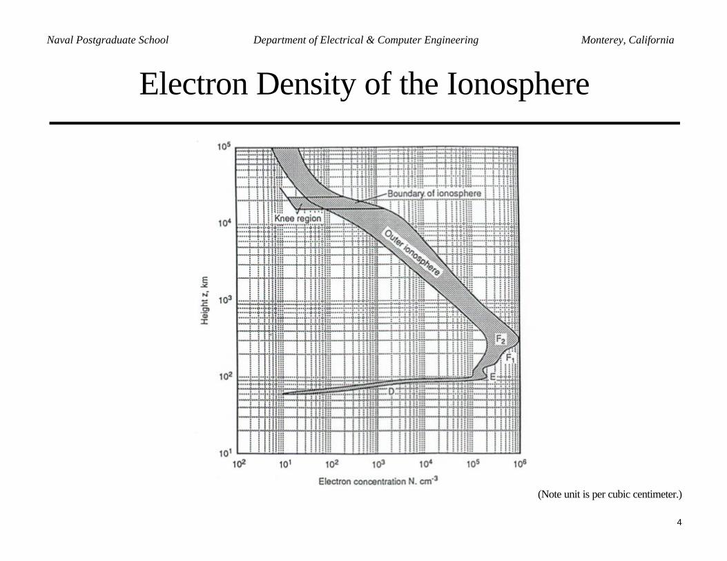
The electron density distribution has the general characteristics shown on the next page. Thedetailed features vary with
• location on Earth,• time of day,• time of year, and• sunspot activity.
The regions around peaks in the density are referred to as layers. The F layer often splitsinto the 1F and 2F layers.
4
Naval Postgraduate School Department of Electrical & Computer Engineering Monterey, California
Electron Density of the Ionosphere
(Note unit is per cubic centimeter.)
5
Naval Postgraduate School Department of Electrical & Computer Engineering Monterey, California
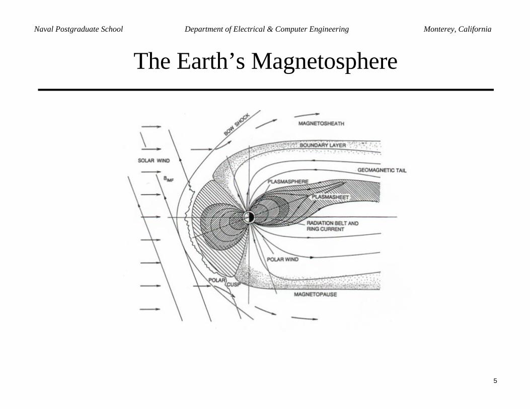
The Earth’s Magnetosphere
6
Naval Postgraduate School Department of Electrical & Computer Engineering Monterey, California
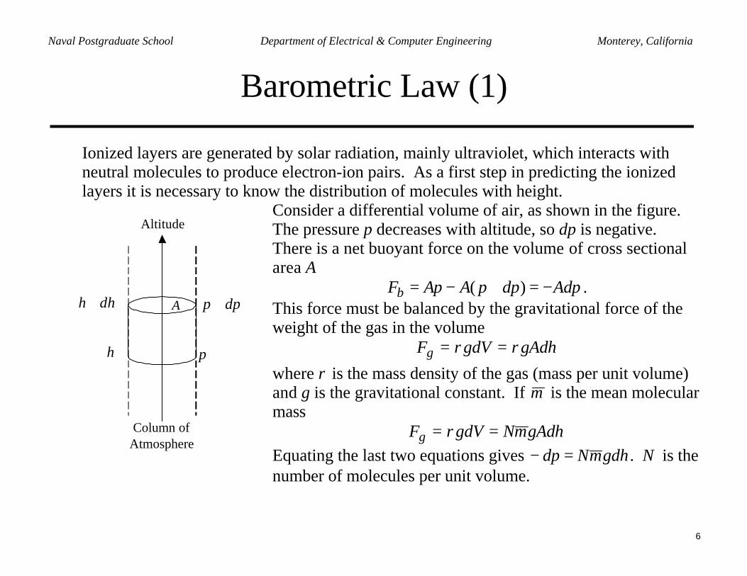
Barometric Law (1)
Ionized layers are generated by solar radiation, mainly ultraviolet, which interacts withneutral molecules to produce electron-ion pairs. As a first step in predicting the ionizedlayers it is necessary to know the distribution of molecules with height.
A
Altitude
Column ofAtmosphere
dhh +
h p
dpp +
Consider a differential volume of air, as shown in the figure.The pressure p decreases with altitude, so dp is negative.There is a net buoyant force on the volume of cross sectionalarea A
AdpdppAApFb −=+−= )( .This force must be balanced by the gravitational force of theweight of the gas in the volume
gAdhgdVFg ρρ ==where ρ is the mass density of the gas (mass per unit volume)and g is the gravitational constant. If m is the mean molecularmass
gAdhmNgdVFg == ρEquating the last two equations gives gdhmNdp =− . N is thenumber of molecules per unit volume.
7
Naval Postgraduate School Department of Electrical & Computer Engineering Monterey, California
Barometric Law (2)
Pressure and temperature are related by the ideal gas law: TNkp = (k is Boltzman’sconstant and T is temperature). Use the ideal gas law to substitute for N in dp:
dhk
gmp
dpT
−=−
then integrate from starting height oh to a final height h
∫ ′=h
ho o
hdk
gmhphp
T)()(
ln
Finally, assuming that all of the quantities are approximately constant over the heights of
concern, and defining a new constant ,T
1k
gmH
= gives the barometric law for pressure vs.
height:
−
−=
∫
′=
∫ ′=
Hhh
hpHhd
hphdk
gmhphp o
o
h
ho
h
ho
oo
exp)(exp)(T
exp)()(
H is called the local scale height and thus the exponent, when normalized by H, is in “Hunits.” The reference height is arbitrary. The pressure, mass density, and number densityare seen to vary exponentially with height difference measured in H units.
8
Naval Postgraduate School Department of Electrical & Computer Engineering Monterey, California
Chapman’s Theory (1)
Chapman was the first to quantify the formation of ionized regions due to flux from thesun. In general we expect ion production to vary as follows:1. Small at high altitudes − solar flux is high, but the number of molecules available for
ionization is small2. Small at low altitudes − the number of molecules available is large, but solar flux is low
due to attenuation at higher altitudes3. High at intermediate altitudes − sufficient number of molecules and flux
Chapman’s derivation proceeds along the following steps:1. Find the amount of flux penetrating to an altitude h.2. By differentiation, find the decrease in flux with incremental height dh.3. The decrease in flux represents absorbed energy. From the result of step 2 an
expression for ion production per unit volume at height h is derived.4. The barometric law is used to find the optical depth at height h (optical depth is a
measure of the opacity of the atmosphere above h). 5. The maximum height of electron-ion production is set as the reference height.6. Assuming equilibrium (no vertical wind) laws of the variation of the electron density
are derived based on the rates of electron production and loss.7. A scaling law is developed so that ionization can be represented by a single variable
rather than two (altitude and solar zenith angle).
9
Naval Postgraduate School Department of Electrical & Computer Engineering Monterey, California
Chapman’s Theory (2)
Only the final results are presented here. S denotes the solar flux and χ is the zenith angle.The electron density at height h and zenith angle χ is given by
( )
−−= −z
oe ezNhN χχ sec121
exp),(
where Hhhz o /)( −= and oN is the electrondensity at the reference height oh . This equationspecifies a recombination type of layer (as opposedto an attachment type layer1). It can be rewritten(by a substitution of variables and rescaling) as
)secln,0(cos),( χχχ −= zNzN ee
The value for any χ can be obtained from theo0=χ curve.
A
Column ofAtmosphere
dhh +
h
χ
dSS +
S
1There are several reactions which can remove electrons from the ionosphere. The two most important classes of recombination are (1) theelectron attaches itself to a positive ion to form a neutral molecule, and (2) it attaches itself to a neutral molecule to form a negative ion.
10
Naval Postgraduate School Department of Electrical & Computer Engineering Monterey, California
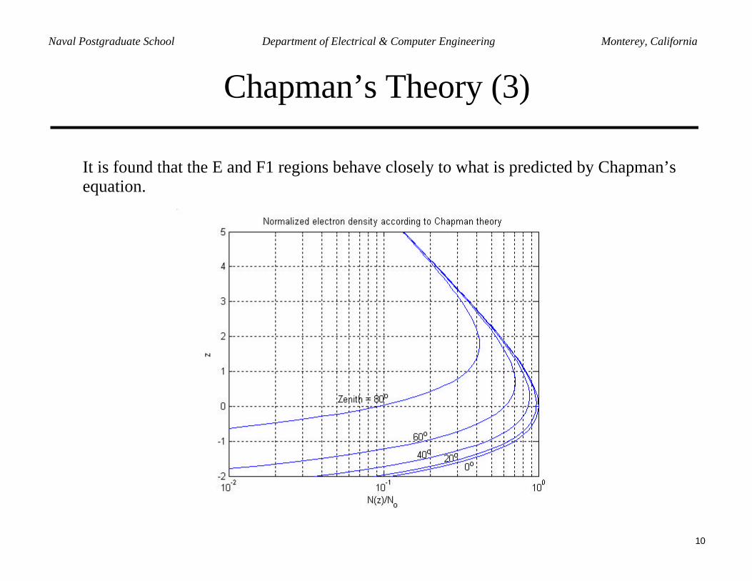
Chapman’s Theory (3)
It is found that the E and F1 regions behave closely to what is predicted by Chapman’sequation.
11
Naval Postgraduate School Department of Electrical & Computer Engineering Monterey, California
Dielectric Constant of a Plasma (1)
When an electric field is applied, charges in the ionosphere are accelerated. The mass ofthe ions (positive charges) is much greater than the electrons, and therefore the motion ofthe ions can be neglected in comparison with that of the electrons. The polarization vectoris
deNpNP eerrr
−=−=
where =eN electron density 3m/ , 191059.1 −×=e C, electron charge, and dr
is theaverage displacement vector between the positive and negative charges. The relativedielectric constant is
EP
EPE
ED
oo
o
or r
rr
rrr
r
εεε
εε +=
+== 1
The propagation constant is
njkc
jjk orc === εω
γ
where rn ε= is the index of refraction. Both the dielectric constant and index ofrefraction can be complex ( rrr jεεε ′′−′= and njnn ′′−′= ).
12
Naval Postgraduate School Department of Electrical & Computer Engineering Monterey, California
Dielectric Constant of a Plasma (2)
Assume a x polarized electric field. The electrons must follow the electric field, andtherefore, xxd ˆ=
r. The equation of motion of an electron is
tjxeeExmxm ων −=+ &&&
where 31100.9 −×=m kg, electron mass, and =ν collision frequency. The solution of theequation of motion is of the form tjaex ω= . Substituting this back into the equation gives
tjx
tjtj eeEaejmeam ωωω ωνω −=+− )()( 2
with ( )ωνω /12 jm
eEa x
−= . The polarization vector is
( )ωνω
ω
/1
ˆ2
2
jm
xeEeNP
tjxe
−−=
r
Now define a plasma frequency, o
ep m
eNε
ω2
= and constants 2
=
ω
ω pX and ων
=Z so
that
( )jZX
xeEP tjxo −
−=1
ˆωεr
.
13
Naval Postgraduate School Department of Electrical & Computer Engineering Monterey, California
Dielectric Constant of a Plasma (3)
The ratio of Pr
to Er
gives the complex dielectric constant, which is equal to the square ofthe index of refraction
( ) ( )νωω
ωεεε
jjZX
nj prrr −
−=−
−==′′−′=2
2 11
1
Separating into real and imaginary terms gives an equivalent conductivity o
rr jωε
σεε −′=
where
( )22
21
ωνεε
+−=′
m
eN
o
er and ( )22
2
ων
νσ
+=
m
eNe
For the special case of no collisions, 0=ν , and the corresponding propagation constantis real
2
2
1ω
ωεεµω p
ooroc kk −==
with oook εµω= .
14
Naval Postgraduate School Department of Electrical & Computer Engineering Monterey, California
Dielectric Constant of a Plasma (4)
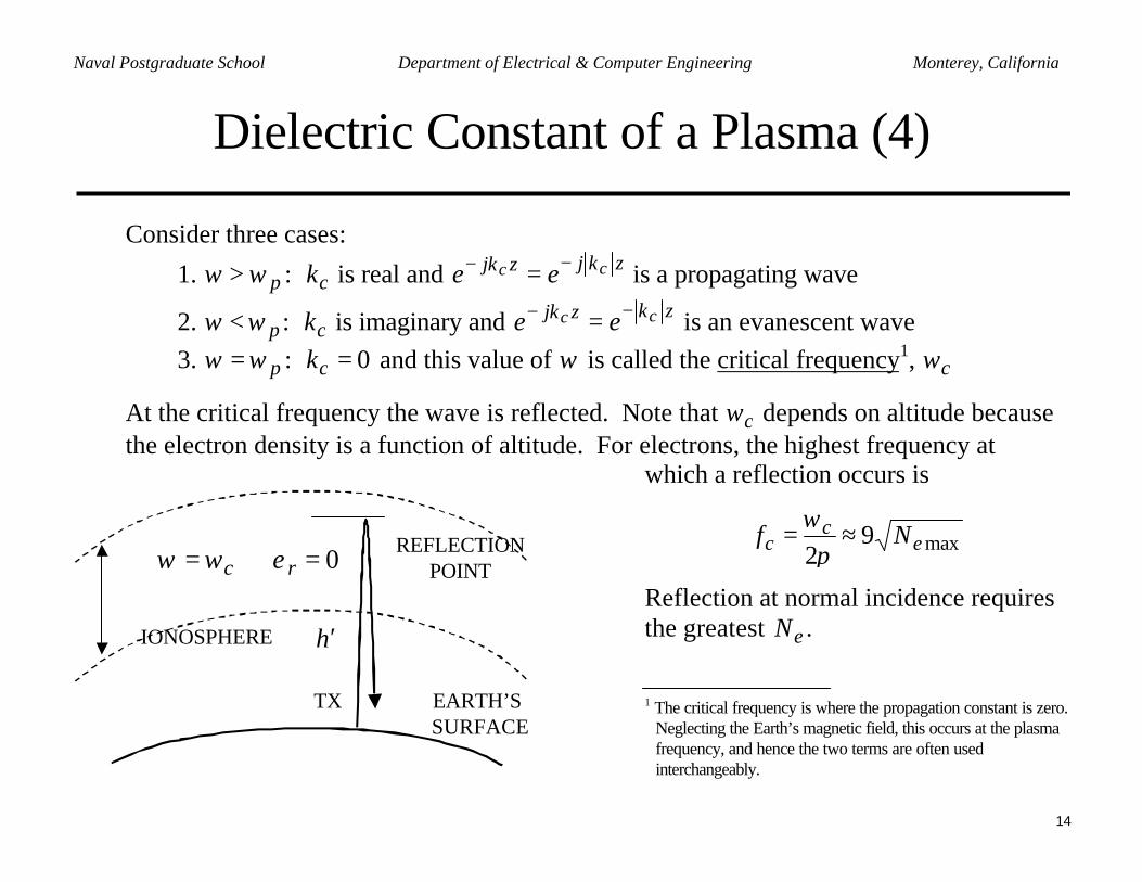
Consider three cases:
1. pωω > : ck is real and zkjzjk cc ee −− = is a propagating wave
2. pωω < : ck is imaginary and zkzjk cc ee −− = is an evanescent wave3. pωω = : 0=ck and this value of ω is called the critical frequency1, cω
At the critical frequency the wave is reflected. Note that cω depends on altitude becausethe electron density is a function of altitude. For electrons, the highest frequency at
EARTH’S SURFACE
TX
IONOSPHERE h′
REFLECTIONPOINT0=⇒= rc εωω
which a reflection occurs is
max92 e
cc Nf ≈=
πω
Reflection at normal incidence requiresthe greatest eN .
1 The critical frequency is where the propagation constant is zero.Neglecting the Earth’s magnetic field, this occurs at the plasmafrequency, and hence the two terms are often usedinterchangeably.
15
Naval Postgraduate School Department of Electrical & Computer Engineering Monterey, California
Ionospheric Radiowave Propagation (1)
If the wave’s frequency and angle of incidence on the ionosphere are chosen correctly,the wave will curve back to the surface, allowing for very long distance communication.For oblique incidence, at a point of the ionosphere where the critical frequency is cf ,the ionosphere can reflect waves of higher frequencies than the critical one. When thewave is incident from a non-normal direction, the reflection appears to occur at a virtualreflection point, h ′, that depends on the frequency and angle of incidence.
EARTH’S SURFACETX
IONOSPHERE
h′
VIRTUALHEIGHT
SKIP DISTANCE
16
Naval Postgraduate School Department of Electrical & Computer Engineering Monterey, California
Ionospheric Radiowave Propagation (2)
To predict the bending of the ray we use a layered approximation to the ionosphere just aswe did for the troposphere.
1z2z3z
1ψ
iψ
2ψ3ψ
AL
TIT
UD
E
LAYEREDIONOSPHERE
APPROXIMATION)( 1zrε)( 2zrε)( 3zrε
M
1=rε
Snell’s law applies at each layer boundary
( ) L== )(sinsin 11 zri εψψ
The ray is turned back when 2/)( πψ =z , or )(sin zri εψ =
17
Naval Postgraduate School Department of Electrical & Computer Engineering Monterey, California
Ionospheric Radiowave Propagation (3)
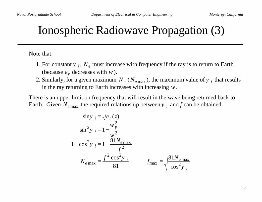
Note that:
1. For constant iψ , eN must increase with frequency if the ray is to return to Earth(because rε decreases with ω ).
2. Similarly, for a given maximum eN ( maxeN ), the maximum value of iψ that resultsin the ray returning to Earth increases with increasing ω .
There is an upper limit on frequency that will result in the wave being returned back toEarth. Given maxeN the required relationship between iψ and f can be obtained
i
eie
ei
pi
ri
Nf
fN
f
N
z
ψ
ψ
ψω
ωψ
εψ
2max
max
22
max
2max2
2
22
cos
8181
cos
811cos1
1sin
)(sin
=⇒=
−=−
−=
=
18
Naval Postgraduate School Department of Electrical & Computer Engineering Monterey, California
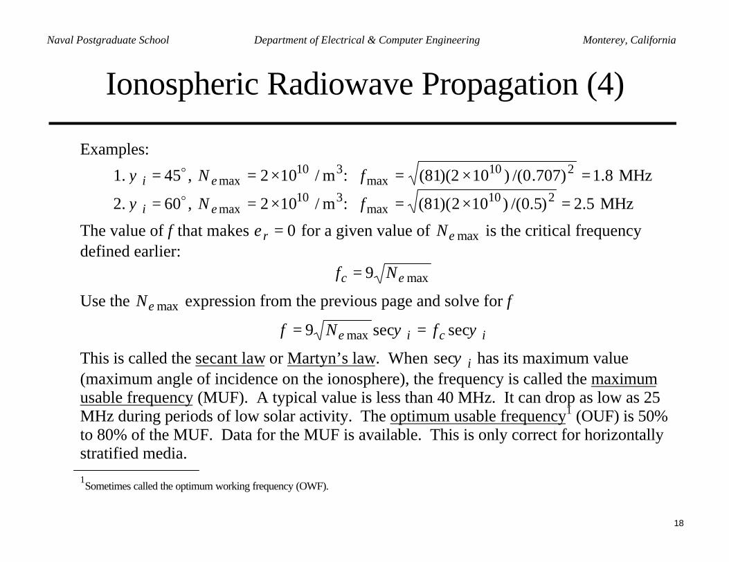
The value of f that makes 0=rε for a given value of maxeN is the critical frequencydefined earlier:
max9 ec Nf =
Use the maxeN expression from the previous page and solve for f
icie fNf ψψ secsec9 max ==
This is called the secant law or Martyn’s law. When iψsec has its maximum value(maximum angle of incidence on the ionosphere), the frequency is called the maximumusable frequency (MUF). A typical value is less than 40 MHz. It can drop as low as 25MHz during periods of low solar activity. The optimum usable frequency1 (OUF) is 50%to 80% of the MUF. Data for the MUF is available. This is only correct for horizontallystratified media.1Sometimes called the optimum working frequency (OWF).
19
Naval Postgraduate School Department of Electrical & Computer Engineering Monterey, California
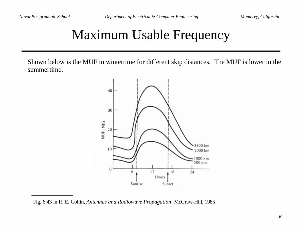
Maximum Usable Frequency
Shown below is the MUF in wintertime for different skip distances. The MUF is lower in thesummertime.
Fig. 6.43 in R. E. Collin, Antennas and Radiowave Propagation, McGraw-Hill, 1985
20
Naval Postgraduate School Department of Electrical & Computer Engineering Monterey, California
Ionospheric Radiowave Propagation (5)
Multiple hops allow for very long range communication links (transcontinental). Using asimple flat Earth model, the virtual height (h ′), incidence angle ( iψ ), and skip distance (d )
are related by hd
i ′=
2tanψ . This implies that the wave is launched well above the horizon.
However, if a spherical Earth model is used and the wave is launched on the horizon thenhRd e ′′= 22 .
EFFECTIVE SPECULARREFLECTION POINT
IONOSPHERE
ψ i
′ h
d
Single ionospheric hop(flat Earth)
EARTH’S SURFACE
TX
IONOSPHERE
Multiple ionospheric hops(curved Earth)
21
Naval Postgraduate School Department of Electrical & Computer Engineering Monterey, California
Ionospheric Radiowave Propagation (6)
Approximate virtual heights for layers of the ionosphere
Layer Range for h ′ (km)2F 250 to 400 (day)
1F 200 to 250 (day)F 300 (night)E 110
Example: Based on geometry, a rule of thumb for the maximum incidence angle on theionosphere is about o74 . The MUF is
cc ff 6.3)74sec(MUF == o
For 312max m/10=eN , 9≈cf MHz and the 4.32MUF = MHz. For reflection from the 2F
layer, 300≈′h km. The maximum skip distance will be about
4516)10300)(108500(2222 33max =××=′′≈ hRd e km
22
Naval Postgraduate School Department of Electrical & Computer Engineering Monterey, California
Ionospheric Radiowave Propagation (7)
For a curved Earth, using the law of sines for a triangle i
eRhψθ
θtan
1sin
cos/1=
−′′+
R/2h′
d / 2
θ
eR′
φ
ψi
LAUNCH ANGLE:
90o
−θ −ψ i = φ − 90o
∆ =
∆
R/2
where
eRd
′=
2θ
and the launch angle (antennapointing angle above the horizon)is
iψθφ −−=−=∆ oo 9090
The great circle path via thereflection point is R, which can beobtained from
i
eRR
ψθ
sinsin2 ′
=
23
Naval Postgraduate School Department of Electrical & Computer Engineering Monterey, California
Ionospheric Radiowave Propagation (8)
Example: Ohio to Europe skip (4200 miles = 6760 km). Can it be done in one hop?
To estimate the hop, assume that the antenna is pointed on the horizon. The virtual height required for the total distance is
( ) 3976.02/2/ =′=→′= ee RdRd θθ rad = 22.8 degrees720/coscos)( =′−′=′→′=′+′ eeee RRhRhR θθ km
This is above the F layer and therefore two skips must be used. Each skip will be half ofthe total distance. Repeating the calculation for 16902/ =d km gives
( ) 1988.02/ =′= eRdθ rad = 11.39 degrees711/cos =′−′=′ ee RRh θ km
This value lies somewhere in the F layer. We will use 300 km (a more typical value) incomputing the launch angle. That is, still keep 16902/ =d km and θ = 11.39 degrees, butpoint the antenna above the horizon to the virtual reflection point at 300 km
ooo 4.74)39.11cos(8500300
1)39.11sin(tan1
=→
−+=
−
ii ψψ
24
Naval Postgraduate School Department of Electrical & Computer Engineering Monterey, California
Ionospheric Radiowave Propagation (9)
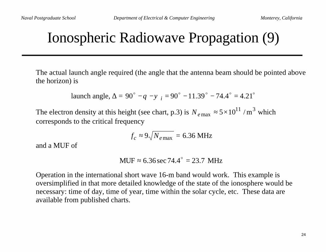
The actual launch angle required (the angle that the antenna beam should be pointed abovethe horizon) is
The electron density at this height (see chart, p.3) is 311max m/105×≈eN which
corresponds to the critical frequency
=≈ max9 ec Nf 6.36 MHzand a MUF of
7.234.74sec36.6MUF =≈ o MHz
Operation in the international short wave 16-m band would work. This example isoversimplified in that more detailed knowledge of the state of the ionosphere would benecessary: time of day, time of year, time within the solar cycle, etc. These data areavailable from published charts.
25
Naval Postgraduate School Department of Electrical & Computer Engineering Monterey, California
Ionospheric Radiowave Propagation (10)
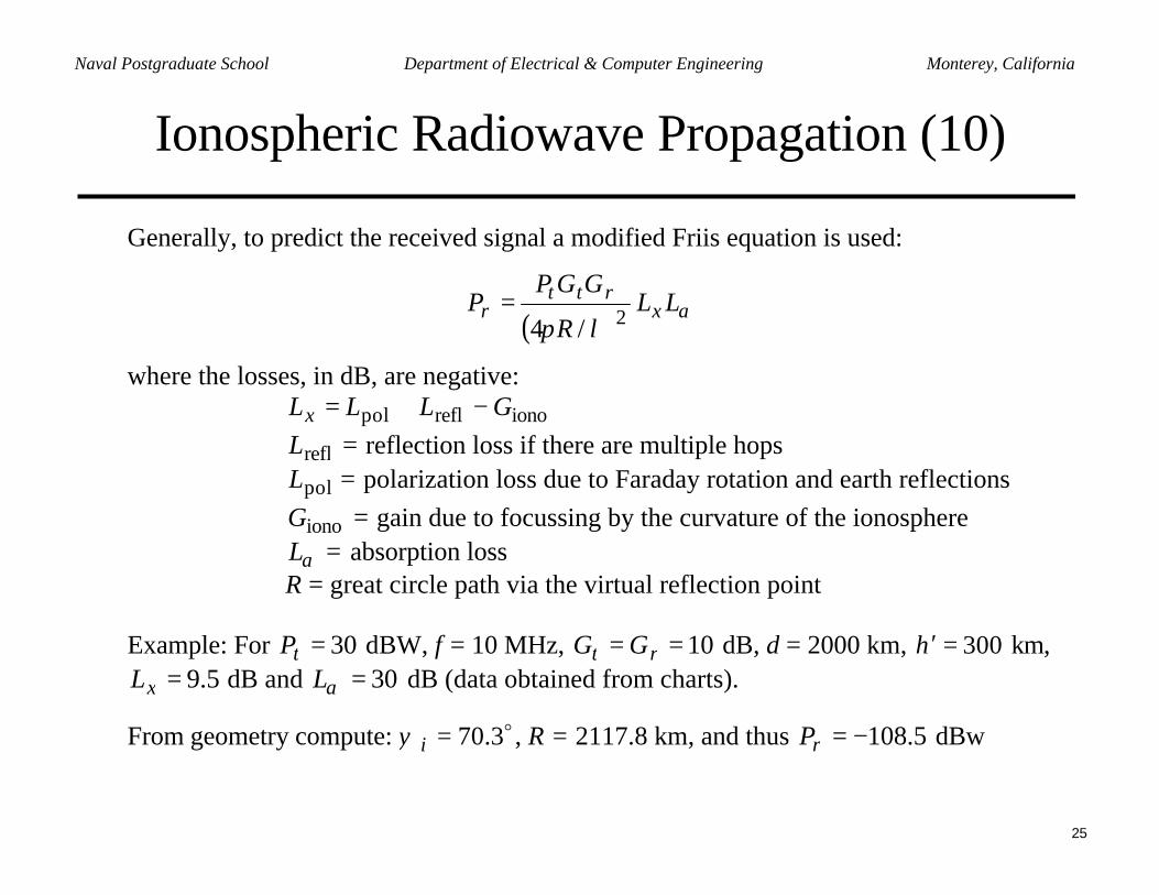
Generally, to predict the received signal a modified Friis equation is used:
( ) αλπ
LLR
GGPP x
rttr 2/4
=
where the losses, in dB, are negative:ionoreflpol GLLLx −+=
=reflL reflection loss if there are multiple hops=polL polarization loss due to Faraday rotation and earth reflections=ionoG gain due to focussing by the curvature of the ionosphere
=αL absorption lossR = great circle path via the virtual reflection point
Example: For 30=tP dBW, f = 10 MHz, 10== rt GG dB, d = 2000 km, 300=′h km,5.9=xL dB and 30=αL dB (data obtained from charts).
From geometry compute: o3.70=iψ , R = 2117.8 km, and thus 5.108−=rP dBw
26
Naval Postgraduate School Department of Electrical & Computer Engineering Monterey, California
Magneto-ionic Medium (1)
Thus far the Earth’s magnetic field has been ignored. An electron with velocity ur movingin a medium with a magnetic field ooo HB
rrµ= experiences a force om BueF
rrr×−= .
Assume a plane wave that is propagating in the z direction ( zeHE γ−~,rr
). From Maxwell’sequations
[ ]( )( )
( )
=+=+=+=
→+==×∇)3(0)2(/)1(/
zzzo
yyoyx
xxoxy
o
DjPEjEPEjHEPEjH
PEjDjHωεω
εωγεωγ
εωωrrrr
−==
−=→−=×∇
)6(0)5()4(
zo
yox
xoy
o
HjHjE
HjEHjE
ωµωµγ
ωµγωµ
rr
These equations show that the plane wave will be transverse only with respect to the Br
, Dr
and Hr
vectors, which is different from the isotropic case. The characteristic impedance ofthe medium is
γωµη /// oxyyx jHEHE =−== .
27
Naval Postgraduate School Department of Electrical & Computer Engineering Monterey, California
Magneto-ionic Medium (2)
Solve (5) for yH and use the result in (1): 43421
2
122
n
EP
xo
xoo
+−=
εεµωγ . A similar process
starting with equation (4) would lead to yo
y
E
Pn
ε+=12 . Equating this to the expression for
2n above gives the polarization ratio of the wave, y
x
y
xEE
PP
R =≡pol .
Rewrite the equation of motion for an average electron when both electric and magneticfields are present
( )oBrEermrmr&rr&r&&r ×+−=+ν
There is also a term in the parenthesis for the magnetic field of the wave, but it turns out tobe negligible. We now define the longitudinal and transverse components, which areparallel and perpendicular to the direction of propagation, respectively.
28
Naval Postgraduate School Department of Electrical & Computer Engineering Monterey, California
Magneto-ionic Medium (3)
Definition of the coordinate system: y lies in the plane defined by )( ooo HB µ= and z
)transverse(sin)allongitudin(cos
θθ
oyT
ozLHHHHHH
====
Note the direction of x is chosen to forma right-handed system (RHS). Anycombination of propagation directionand magnetic field can be handled withthis convention, as long as they are notparallel. If they are parallel anycombination of x and y that forms aRHS is acceptable.
x
y
Direction ofpropagation
oBr
Lies in the planedefined by z and BoEarth’s magnetic
field vector
LBr
TBr
Determinedfrom z and y
z
θ
In this coordinate system the equation of motion can be written as three scalar equations,which for the x component is
( )ToLox HzHyEexmxm µµν &&&&& −+−=+
29
Naval Postgraduate School Department of Electrical & Computer Engineering Monterey, California
Magneto-ionic Medium (4)
For time-harmonic displacements, phasors can be used and the derivatives in time give amultiplicative factor ωj
( )ToLox HzjHyjEemxjmx µωµωωνω −+−=+− 2
The polarization is caused by the electron displacements in x, y, and z
e
z
e
y
e
xeNP
zeN
Py
eNP
x−
=−
=−
= ,,
Substituting: e
Tzo
e
Lyox
e
x
e
xeN
HPjeN
HPjeE
eNmPj
eNmP ωµωµωνω
+−−=−2
Multiply by mo /ε and define the longitudinal and transverse gyro-frequencies1:
θωµω cos/ BLoL meH =≡θωµω sin/ BToT meH =≡ .
1In general, the gyro-frequency (also called the cyclotron frequency) of an electron in a magnetic field is defined as meBoB /≡ω or
mHe ooH /µω ≡ .
30
Naval Postgraduate School Department of Electrical & Computer Engineering Monterey, California
Magneto-ionic Medium (5)
For convenience we define the frequency ratios2
=
ω
ω pX , ω
ωLLY = ,
ωωT
TY = , and ων
=Z .
Recall that the plasma frequency is o
ep m
eNε
ω2
= . With this notation
zTyLxxo PjYPjYjZPXE +−−−= )1(ε
Going back to the y and z components of the equation of motion, and treating them thesame, gives two more equations
xTzzo
xLyyoPjYjZPXEPjYjZPXE
−−−=+−−=
)1()1(
εε
These are the equations needed to find n in terms of the components of Er
, and Pr
.Arbitrarily we choose to solve for yP and yE , eliminating zzxx EPEP ,,, .
31
Naval Postgraduate School Department of Electrical & Computer Engineering Monterey, California
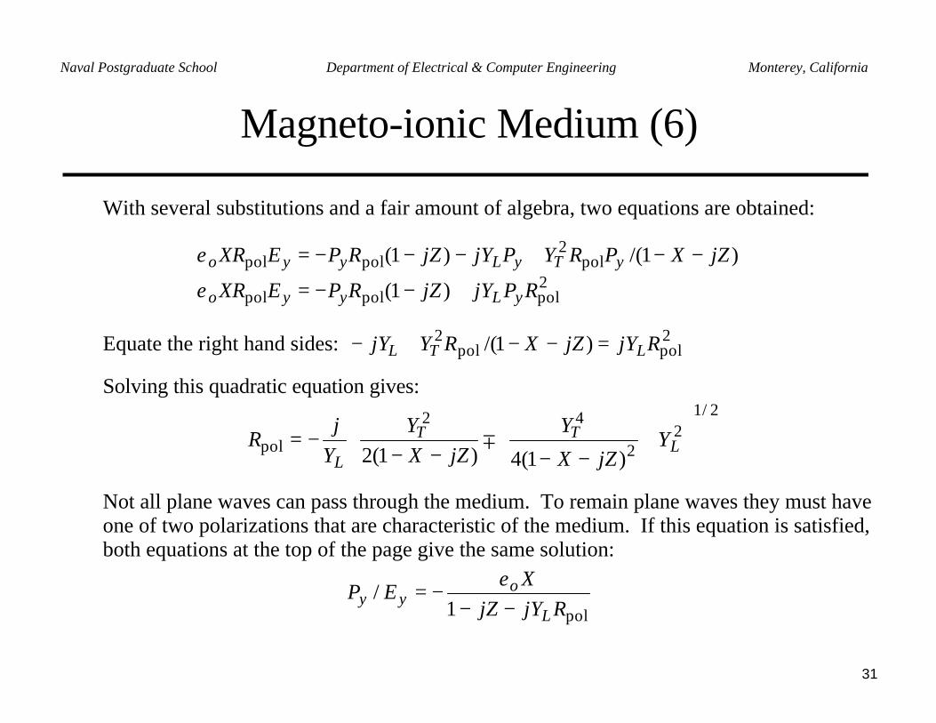
Magneto-ionic Medium (6)
With several substitutions and a fair amount of algebra, two equations are obtained:
2polpolpol
pol2
polpol
)1(
)1/()1(
RPjYjZRPEXR
jZXPRYPjYjZRPEXR
yLyyo
yTyLyyo
+−−=
−−+−−−=
ε
ε
Equate the right hand sides: 2polpol
2 )1/( RjYjZXRYjY LTL =−−+−
Solving this quadratic equation gives:
+
−−−−−=
2/12
2
42
pol)1(4)1(2 L
TT
LY
jZX
YjZX
YYj
R ∓
Not all plane waves can pass through the medium. To remain plane waves they must haveone of two polarizations that are characteristic of the medium. If this equation is satisfied,both equations at the top of the page give the same solution:
pol1/
RjYjZX
EPL
oyy −−
−=ε
32
Naval Postgraduate School Department of Electrical & Computer Engineering Monterey, California
Magneto-ionic Medium (7)
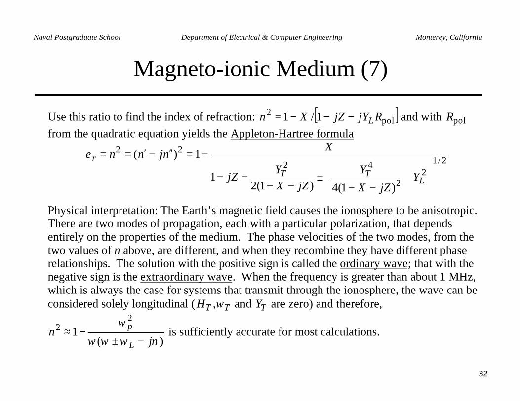
Use this ratio to find the index of refraction: [ ]pol2 1/1 RjYjZXn L−−−= and with polR
from the quadratic equation yields the Appleton-Hartree formula
2/12
2
42
22
)1(4)1(21
1)(
+−−
±−−
−−
−=′′−′==
LTT
r
YjZX
YjZX
YjZ
Xnjnnε
Physical interpretation: The Earth’s magnetic field causes the ionosphere to be anisotropic.There are two modes of propagation, each with a particular polarization, that dependsentirely on the properties of the medium. The phase velocities of the two modes, from thetwo values of n above, are different, and when they recombine they have different phaserelationships. The solution with the positive sign is called the ordinary wave; that with thenegative sign is the extraordinary wave. When the frequency is greater than about 1 MHz,which is always the case for systems that transmit through the ionosphere, the wave can beconsidered solely longitudinal ( TH , Tω and TY are zero) and therefore,
)(1
22
νωωω
ω
jn
L
p
−±−≈ is sufficiently accurate for most calculations.
33
Naval Postgraduate School Department of Electrical & Computer Engineering Monterey, California
Anisotropic Media
In an isotropic medium the phase velocity at any given point is independent of thedirection of propagation. For an anisotropic medium, the direction of phase propagation(i.e., movement of the equiphase planes) differs, in general, from that of energypropagation.
Isotropic Medium Anisotropic Medium
NoncircularWavefront
PrPoint
Source
RayDirection(Radial)
WavefrontNormal
oBrφ
CircularWavefront
P
r
PointSource
34
Naval Postgraduate School Department of Electrical & Computer Engineering Monterey, California
Phase Velocity and Time Delay (1)
The time delay between a transmitter at P1 and receiver at P2 is: ∫ ′=
2
1)(
11 P
Pd ds
snct
The angular (radian) phase path length is: ∫ ′=Φ2
1
)(P
Pdssn
cω
.
Let the distance between point P1 and P2 be l . As a check, for a homogeneous medium
ll βεω
==Φ rc
The phase velocity is βω
=pu , which can be determined once β is known. The group
velocity is βω
dd
ug = . The velocity of energy propagation is generally taken as the group
velocity1. It is always true that 2cuu gp = .
1This is the velocity of propagation of a packet of frequencies centered about a carrier frequency. For simple amplitude modulated (AM) waveforms, it
is the velocity of propagation of the envelope, whereas the phase velocity is the velocity of propagation of the carrier.
35
Naval Postgraduate School Department of Electrical & Computer Engineering Monterey, California
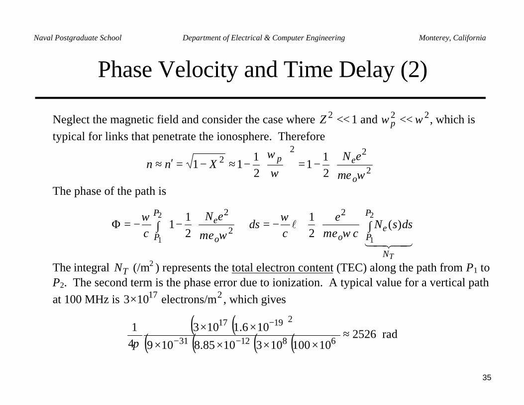
Phase Velocity and Time Delay (2)
Neglect the magnetic field and consider the case where 12 <<Z and 22 ωω <<p , which istypical for links that penetrate the ionosphere. Therefore
−=
−≈−=′≈ 2
222
21
121
11ωεω
ω
o
ep
m
eNXnn
The phase of the path is
43421l
TN
P
Pe
o
P
P o
e dssNcm
ec
dsm
eNc
∫
+−=∫
−−=Φ
2
1
2
1
)(21
21
12
2
2
ωεω
ωε
ω
The integral TN (/m2 ) represents the total electron content (TEC) along the path from P1 toP2. The second term is the phase error due to ionization. A typical value for a vertical pathat 100 MHz is 217 melectrons/ 103× , which gives
( )( )( )( )( )( ) rad 2526
101001031085.8109106.1103
41
681231
21917≈
××××××
−−
−
π
36
Naval Postgraduate School Department of Electrical & Computer Engineering Monterey, California
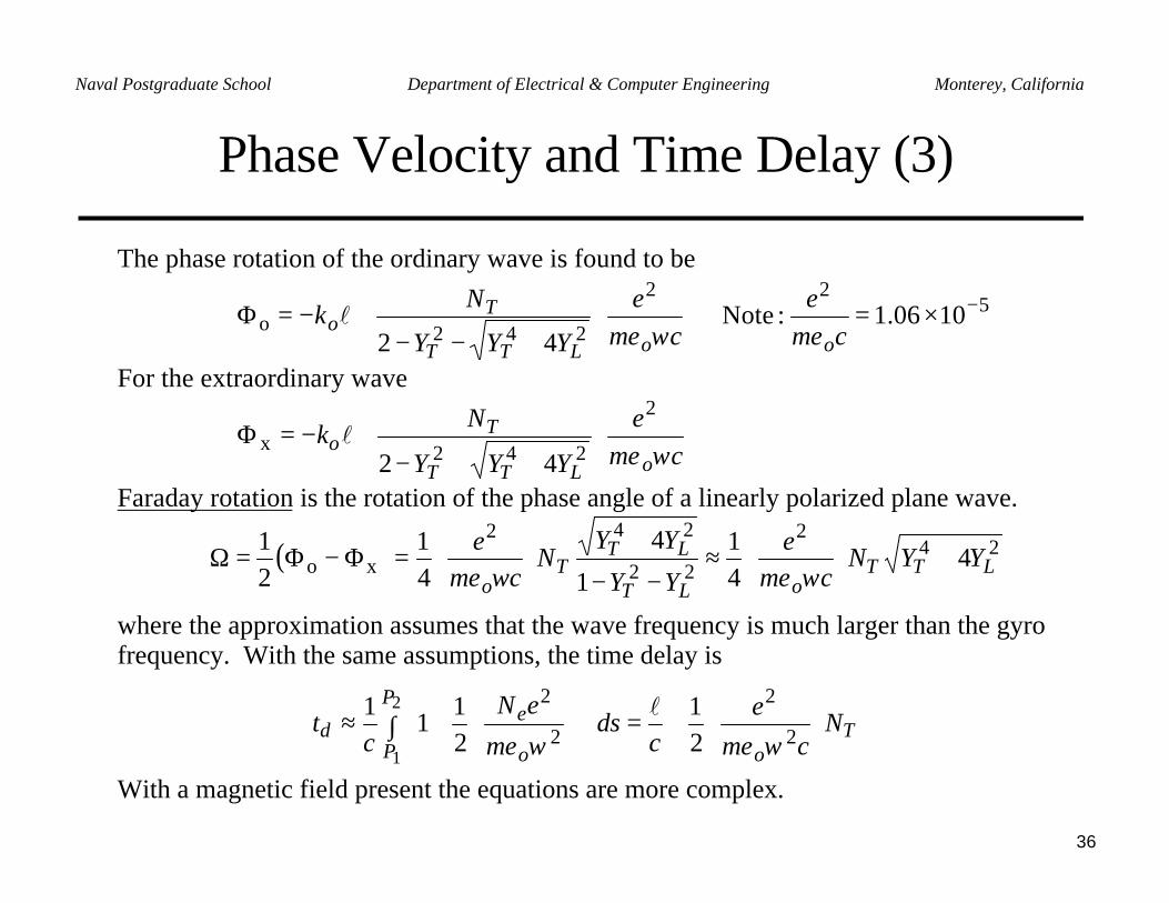
Phase Velocity and Time Delay (3)
The phase rotation of the ordinary wave is found to be
522
242o 1006.1:Note42
−×=
+−−+−=Φ
cme
cme
YYY
Nk
ooLTT
To εωεl
For the extraordinary wave
++−+−=Φ
cme
YYY
Nk
oLTT
To ωε
2
242x42
l
Faraday rotation is the rotation of the phase angle of a linearly polarized plane wave.
( ) 242
22
242
xo 441
1
441
21
LTToLT
LTT
oYYN
cme
YY
YYN
cme
+
≈
−−
+
=Φ−Φ=Ω
ωεωε
where the approximation assumes that the wave frequency is much larger than the gyrofrequency. With the same assumptions, the time delay is
To
P
P o
ed N
cme
cds
m
eNc
t
+=∫
+≈ 2
2
2
2
21
21
11 2
1 ωεωεl
With a magnetic field present the equations are more complex.
37
Naval Postgraduate School Department of Electrical & Computer Engineering Monterey, California
Example
Find the Faraday rotation of a 135 MHz plane wave propagating a distance of 200 kmthrough the ionosphere. The electron density is constant over the path and equal to
10105× /m3. The gyro-frequency is 6108× Hz. Assume collisions can be neglected andthat the propagation is longitudinal.
The TEC is ( ) 16103
01010510200)( =××=∫ == eeT NdssNN l
l /m2. For longitudinal
propagation and no collisions 0== ZYT and ωω /BLY =
( )( )( )( )( )
radians75.31013522
1082101006.1
241
26
6165
2
≈×
××≈
≈Ω
−
π
π
ωω
ωεB
To
Ncm
ex x
y yinE
r
outEr z
200 km
3.75 rad
38
Naval Postgraduate School Department of Electrical & Computer Engineering Monterey, California
Absorption
Once the index of refraction is determined for the medium, the attenuation constant can beobtained from
nc
jjω
βαγ =+= .
For simplicity, the effect of the magnetic field is ignored in this discussion ( 0== LT YY ) sothat
+−
+−=′′−′= 22
22
111)(
ZXZ
jZ
Xnjnn
yielding 2121
Z
XZnc
nc +′
=′′=ωω
α . In general, α is not constant along a path through the
ionosphere, because the electron density, and hence X and n′ are changing along the path.The collision frequency, if not zero, can also change with location in the ionosphere. Thus,the loss due to absorption from 1P to 2P should be computed from
∫−=2
1
)(expattn
P
PdssL α
where s is the distance along the path.
39
Naval Postgraduate School Department of Electrical & Computer Engineering Monterey, California
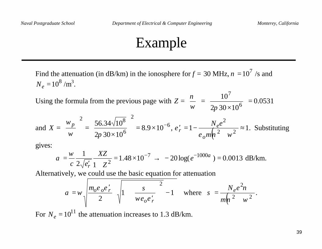
Example
Find the attenuation (in dB/km) in the ionosphere for f = 30 MHz, 710=ν /s and810=eN /m3.
Using the formula from the previous page with 0531.010302
106
7=
×=
=
πων
Z
and 62
6
82
109.810302
1034.56 −×=
×=
=
πω
ωpX , ( ) 11 22
2≈
+−=′
ωνεε
m
eN
o
er . Substituting
gives:
→×=+′
= −72 1048.1
121
Z
XZec r
ωα 0013.0)log(20 1000 =− − αe dB/km.
Alternatively, we could use the basic equation for attenuation
−
′
+′
= 112
2
ro
roo
εωεσεεµ
ωα where ( )22
2
ων
νσ
+=
m
eNe .
For 1110=eN the attenuation increases to 1.3 dB/km.