Satellite Constellation Assessment Study Using Dual Radio Occultation and Microwave Radiometry Observations
David D. Morabito,* Chi Ao,† Joseph Turk,‡ and Stephen Lowe†
ABSTRACT. — The use of constellations involving closely spaced low–Earth orbiting (LEO) satellites provides advantages allowing for improvement in understanding basic cloud convective processes. One can achieve several advantages by collecting successive radio occultation measurements using such a constellation of closely spaced LEO satellites that receive transmissions from global navigation satellite system (GNSS) constellations. These observations can be complemented with concurrent microwave radiometry measurements. We assess the relative performance of employing different satellite constellations in acquiring such measurements, with the aim of maximizing coverage over longitude and latitude and over short data-acquisition periods. Considerations for orbit strategies include the number of satellites, the spacing of the satellites, and the number of strings or orbital planes. We performed simulations involving different constellations (orbit strategies) to assess opportunities where radio occultation events lie within a given threshold relative to nadir-pointed microwave radiometry measurements. We also considered the number of participating GNSS constellations, such as Global Positioning System (GPS), Galileo, and Global Navigation Satellite System (GLONASS), as well as the number of days for analysis over which the observations were acquired.
I. Introduction
Constellations consisting of closely spaced low–Earth orbiting (LEO) satellites provide advantages in collecting information, allowing for improved understanding of basic cloud convective processes. Up to now, it has been difficult to obtain important observations dealing with accurate meteorological quantities in the vicinity of convective clouds [1]. One can achieve such advantages by collecting successive radio occultation (RO) measurements using a constellation of closely spaced LEO satellites that receive transmissions from global navigation satellite system (GNSS) constellations, complemented by concurrent microwave radiometry (MW) measurements.
2
Successive RO signal links can spatially sample different regions of air masses lying within and outside areas of high precipitation. A sequence of such RO links would allow some of these to intersect regions of heavy precipitation while others intersect regions that have less or are devoid of precipitation. In addition, by making use of two orthogonal polarizations, the RO measurements allow for the detection of heavy precipitation regions, as demonstrated by the Paz spacecraft [2]. The addition of nadir-pointed multifrequency passive microwave radiometers (MW) on the same (or other) satellites allows for collection of water vapor content outside of the regions of clouds and precipitation. The MW measurements therefore complement the RO measurements when made spatially close (in angle) and temporally close to each other. The passive satellite sensors provide pressure, temperature, and water vapor content profiles that allow for the characterization of total columnar water vapor over large regions of longitude-latitude space. In the past, such measurements were mostly available over land, such as those acquired by radiosonde and ground-based radiometry equipment.
Existing passive microwave constellations include those on the National Oceanic and Atmospheric Administration (NOAA) and the European Organisation for the Exploitation of Meteorological Satellites (EUMETSAT) weather satellites that employ Advanced Technology Microwave Sounder (ATMS) sounders. By sampling frequencies along the skirt of the 183.31 GHz water vapor absorption line, one can achieve observations that are sensitive to emission and scattering processes that originate from precipitation-sized ice hydrometeors associated with vertical air motion [3]. The MW data thus provide detail on the horizontal extent and the structure of the convective systems that are traversed or sensed by the RO signals. Total columnar water vapor extracted from MW data, and combined with the RO signal data, could allow for resolving water vapor structure within the boundary layer as opposed to that lying above it in the free troposphere [4].
In this paper, we assess the relative performance of using a variety of different satellite constellations in acquiring the measurements, with the aim of maximizing coverage over longitude-latitude space and over shorter temporal data-acquisition periods. Considerations in the various orbit strategies include the number of satellites, the spacing of the satellites, and the number of strings or orbital planes. We performed simulations involving the different orbit strategies in order to identify the number of and density of opportunities where RO events lie close (within a given threshold) relative to the MW measurement points. Previous work focused on the use of a four-satellite constellation simulation [1], where the RO ray paths were superimposed on actual precipitation field maps. In this paper, we also consider the number of participating GNSS constellations, which could include GPS, Galileo, and GLONASS. We also consider the number of days for analysis over which the observations are acquired.
II. Instrumentation
Each satellite in the constellation carries both RO and passive MW radiometer equipment. In addition, each satellite carries two complementary receiving antennas for the RO links with boresights pointed in both forward and aft directions aligned along the velocity vector. The antennas are modeled with 60° beams (relative to boresight), and thus can receive GNSS signals for both rising and setting occultation events. Each RO event is
3
characterized by the location of the tangent point of the signal path above the Earth’s surface between it and the GNSS transmitting satellite. When the straight-line tangent point between the transmitter and the receiver is 100 km below the surface due to refraction, this will correspond to the signal path roughly grazing the Earth’s surface due to atmospheric refraction. For the purpose of this study, we consider straight-line paths whose tangent points lie ~1 km above the surface, thus neglecting refraction.
We assume that each of the satellites carries passive MW sounding radiometers that operate in the millimeter-wave (183 GHz) water vapor absorption band. In practice, not all of the satellites in a constellation may carry MW equipment, for only satellites in strategically placed orbit locations would carry these. These instruments are sensitive to cloud-top ice regions under conditions of heavy precipitation [3]. Other radiometers that operate in a longer wavelength water vapor band (near 22 GHz, for example) can provide a long record of total columnar water vapor [6]. We assume that these instruments have a ±45° beam shape in the cross-direction of the satellite velocity vector which translates to swaths of ±4° projected onto the Earth’s surface at the ~500 km altitude of the satellites. Alternatively, some experimenters might opt to use MW measurements from other independently operated meteorological satellites such as National Oceanic and Atmospheric Administration (NOAA) [7].
III. Satellite Constellations
The satellite constellations are assumed to have circular orbits (zero eccentricity), altitudes of ~475 km and inclinations of 45°. The inclination of 45° allows for coverage over the tropics as well as much of the temperate zones. The temporal spacing between adjacent satellites in an orbital plane (or string) typically range from 2 to 3 min. The orbital period of these constellations is ~1.57 h resulting in ~15 orbits per day. The precession rate of about ~3°/day allows for increased coverage of surface area and thus improved sampling over the globe as successive orbits occur. Eight different satellite constellations were examined and are summarized in Table 1. Each string represents an orbital plane. As an example, the notation “1/6/1” in the last column denotes three orbital planes or strings, where the first orbital plane contains one satellite, the second (or central plane) has six satellites, and the third orbital plane has one satellite.
Table 1. Satellite Constellations
Case Number of Sats.
Altitude (km)
Inclination (deg)
Number Strings
Number Each Str
1 8 475 45 3 “1/6/1”
2 6 475 45 3 “1/4/1”
3 4 475 45 3 “1/2/1”
4 7 475 45 3 “2/3/2”
5 8 475 45 1 “0/8/0”
6 16 475 45 2 “8/8”
7 3 500 45 1 “0/3/0”
8 8 475 45 3 “2/5/1”
4
An example of one such constellation is shown in a snapshot of a Satellite Orbit Analysis Program (SOAP) [5] animation depicted in Figure 1. Here Case 4 (see Table 1) has seven satellites distributed over three strings (or orbital planes), where each string intersects the Earth equatorial plane at longitudes of 97.48°, 107.48° and 117.48°, and the separation between individual satellites in a string is ~10° in angle (or ~2 min in time). For the analysis to follow, we are interested in those RO ray paths whose tangent points lie about 1 km from the surface of the Earth to allow for more optimum sampling of the atmosphere.
Figure 1. SOAP depiction of satellite constellation for Case 4 of Table 1. The ray paths from the different
transmitting GPS satellites to one receiving satellite in the constellation are shown in yellow. To minimize clutter
in the plot, we only show the signal links to one satellite (R0) at the instant of the 19:55:30 UTC time stamp.
The satellite constellation orbit configuration file was used as an input to the simulation software. This file specified orbit parameters for each of the six satellites, which included orbital altitude (in all cases we are assuming eccentricity of zero), inclination, longitude of the ascending node, and mean anomaly. We make use of “pseudo” trajectory information of the GNSS constellation available in the software or their input files.
Figure 2 displays snapshots of the SOAP animations of each of the eight satellite constellations shown in Table 1.
5
Figure 2. SOAP depictions of each constellation case examined: a) Case 1, b) Case 2, c) Case 3, d) Case 4,
e) Case 5, f) Case 6, g) Case 7, and h) Case 8 (see Table 1). Line-of-sight paths to “visible” GPS transmitting
satellites are shown for only receiver satellite (R0) to minimize “clutter”.
6
IV. Simulation Generation Approach
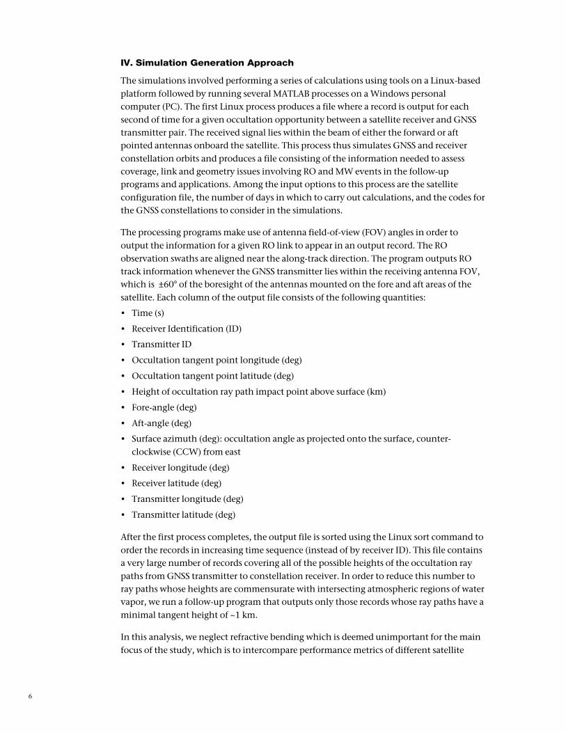
The simulations involved performing a series of calculations using tools on a Linux-based platform followed by running several MATLAB processes on a Windows personal computer (PC). The first Linux process produces a file where a record is output for each second of time for a given occultation opportunity between a satellite receiver and GNSS transmitter pair. The received signal lies within the beam of either the forward or aft pointed antennas onboard the satellite. This process thus simulates GNSS and receiver constellation orbits and produces a file consisting of the information needed to assess coverage, link and geometry issues involving RO and MW events in the follow-up programs and applications. Among the input options to this process are the satellite configuration file, the number of days in which to carry out calculations, and the codes for the GNSS constellations to consider in the simulations.
The processing programs make use of antenna field-of-view (FOV) angles in order to output the information for a given RO link to appear in an output record. The RO observation swaths are aligned near the along-track direction. The program outputs RO track information whenever the GNSS transmitter lies within the receiving antenna FOV, which is ±60° of the boresight of the antennas mounted on the fore and aft areas of the satellite. Each column of the output file consists of the following quantities:
• Time (s)
• Receiver Identification (ID)
• Transmitter ID
• Occultation tangent point longitude (deg)
• Occultation tangent point latitude (deg)
• Height of occultation ray path impact point above surface (km)
• Fore-angle (deg)
• Aft-angle (deg)
• Surface azimuth (deg): occultation angle as projected onto the surface, counter-clockwise (CCW) from east
• Receiver longitude (deg)
• Receiver latitude (deg)
• Transmitter longitude (deg)
• Transmitter latitude (deg)
After the first process completes, the output file is sorted using the Linux sort command to order the records in increasing time sequence (instead of by receiver ID). This file contains a very large number of records covering all of the possible heights of the occultation ray paths from GNSS transmitter to constellation receiver. In order to reduce this number to ray paths whose heights are commensurate with intersecting atmospheric regions of water vapor, we run a follow-up program that outputs only those records whose ray paths have a minimal tangent height of ~1 km.
In this analysis, we neglect refractive bending which is deemed unimportant for the main focus of the study, which is to intercompare performance metrics of different satellite
7
constellations. Thus, at this stage, the output file contains records satisfying the ~1 km height criterion for the occultation tangent point along with the time instants corresponding to the specified target heights.
We are interested in sampling heights from ~1 km up to 10 km due to available evidence that there is a relatively smaller but more variable amount of moisture present above the boundary layer, which range from tens to thousands of meters in height. Such moisture, when abundant, can strengthen convection [1]. Thus, we consider occultation swath lengths that range from ±3° on either side (at the ~10 km height) of the ~1 km height impact distance,1 which lies in the center of the occultation swaths.
As previously mentioned, the addition of multichannel nadir-pointed passive MW instruments aboard one or more of the satellites allow for complementing the RO observations. These instruments provide water vapor structure outside of the high precipitation regions. The ±45° fan-shaped beam of the radiometers translates to a ±4° swath in the cross-track direction intersecting the Earth’s surface as viewed from the satellite orbit altitude.
In order to make use of both MW and RO observations, we require positions of Radio Occultation Microwave (RO-MW) pairs to lie sufficiently close to each other to allow for complementary meteorological observations. Thus, it is desired for the satellites to provide spectrometer (MW) measurements in close proximity to the occultation (RO) impact points (~1 km) in both time and angular distance. Given each record in the output file contains both RO and MW positions, one can identify the opportunities using such a simulation. We desire to have such opportunities flagged whenever a receiver position falls within 5° of an RO ray path impact point (1 km altitude). It is impossible for the same RO-MW pair to satisfy this constraint because the distance between them far exceeds 5° for the given orbital geometry. However, the MW nadir-pointed position could come within 5° of the RO impact point involving the same satellite as it advances (or retards) in its orbit in time. Thus, a test is imposed to calculate the position distance between satellite position (radiometer) and occultation ray path impact point position up to 30 min of each other and infer whether their swath centers lie within the 5° threshold. One deficiency of this approach is that we are constrained to use only MW satellite positions corresponding to given RO opportunities of the same satellite in order to estimate relative RO-MW positions. Given that we are only interested in assessing relative coverage performance between different constellations, we deem this is sufficient. For each constellation configuration we examine the distribution of all possible RO-MW pairs satisfying the threshold criterion over longitude-latitude space for the given GNSS constellations and the number of days considered.
A follow-on program produces another file that contains one record for each RO-MW pair satisfying the threshold criterion (redundancies had been removed). A search is performed by considering each occultation location (li, fi) at time instance ti, and MW receiver location opportunity (lj, fj) at time instance tj where j > i. We then calculate the angular separation distance Dq as
1 The impact distance is also known as the height of the tangent point of the occultation ray path above the surface.
8
∆𝜃 = cos!" (sin f# sin f$ +cos f# cos f$ cos,l# − l$./ (1)
If Dq < 5° within the 30 min search window, then we count this opportunity as one RO-MW pair. In most cases, this angle will exceed 5° as the time difference becomes large. Given that most satellite constellations have about 2- to 3-minute separations between successive satellites in a string, and that the strings considered can have up to eight satellites, 30 min suffices as a temporal search window. This program provides a count of the number of RO-MW pairs for calculation in the forward direction, where ti < tj, starts at the beginning of the file. Here, each occultation event at ti is compared with each MW event at tj, where j ranges from i + 1 to n, and where n is the number of records in the file. A similar process is performed starting at the end of the file going backwards in order to calculate the total counts occurring in the reverse direction. We then wish to examine the number of such opportunities as well as how they are distributed over longitude-latitude space. For this study, we focused on counts only in the forward direction, since the counts are reasonably close to that in the reverse direction, and we are focused on only studying relative performance between satellite constellations.
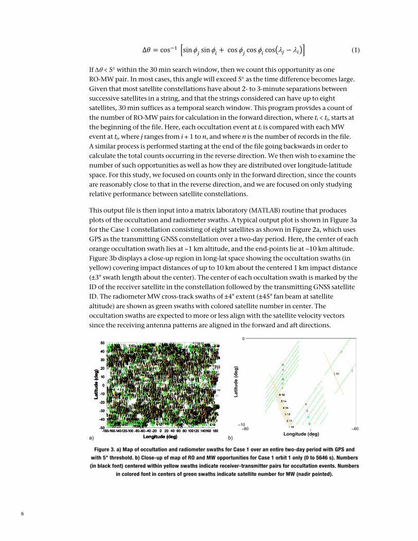
This output file is then input into a matrix laboratory (MATLAB) routine that produces plots of the occultation and radiometer swaths. A typical output plot is shown in Figure 3a for the Case 1 constellation consisting of eight satellites as shown in Figure 2a, which uses GPS as the transmitting GNSS constellation over a two-day period. Here, the center of each orange occultation swath lies at ~1 km altitude, and the end-points lie at ~10 km altitude. Figure 3b displays a close-up region in long-lat space showing the occultation swaths (in yellow) covering impact distances of up to 10 km about the centered 1 km impact distance (±3° swath length about the center). The center of each occultation swath is marked by the ID of the receiver satellite in the constellation followed by the transmitting GNSS satellite ID. The radiometer MW cross-track swaths of ±4° extent (±45° fan beam at satellite altitude) are shown as green swaths with colored satellite number in center. The occultation swaths are expected to more or less align with the satellite velocity vectors since the receiving antenna patterns are aligned in the forward and aft directions.
a) b)
Figure 3. a) Map of occultation and radiometer swaths for Case 1 over an entire two-day period with GPS and
with 5° threshold. b) Close-up of map of RO and MW opportunities for Case 1 orbit 1 only (0 to 5646 s). Numbers
(in black font) centered within yellow swaths indicate receiver-transmitter pairs for occultation events. Numbers
in colored font in centers of green swaths indicate satellite number for MW (nadir pointed).
We can also examine various quantities such as 1) the angular distances between centers of RO and MW swaths; 2) the angles between satellite velocity direction and nearby occultation swaths; and the number of counts for each bin. Here we partition bins in longitude space from -180° to 180° into 20° segments and latitude space of -50° to 50° into 10° segments. Thus, we can examine the opportunities into each 20°´10° bin for these different quantities.
Figure 4a displays the number of RO-MW pairs satisfying the 5° threshold from center-to-center of the RO and MW swaths in each 20°´10° bin. Figure 4b displays the color map equivalent of Figure 4a. The brighter (yellow-white) colors show heavily dense opportunity regions and the darker (red-black) colors show regions that are less dense or devoid of such opportunities. We examine these plots for different satellite configurations to qualitatively compare their relative performance under equivalent assumptions. It is expected that, as the number of GNSS constellations increase and the number of days of observation increase, the longitude-latitude space would be populated with more observations filling the voids and becoming more uniform.
a) b)
Figure 4. a) Density map of number of RO-MW opportunity counts in each 20°´10° cell satisfying 5° threshold
over a two-day period for Case 1; b) Color map displaying number of RO-MW opportunities.
Figure 5 displays a map of average angles between velocity vectors and projected occultation vector directions in each 20°´10° bin for the Case 1 constellation whose numbers are shown in Figure 4 for the GPS constellation over a two-day period (about 30 orbits). Since the forward and aft antenna boresights are centered along the velocity vector, only associated occultation events occurring within the antenna beam are considered. Figure 5b shows the equivalent color map.
Figure 6a displays a density map of the number of distinct GPS transmitters involved in the occultation events in each 20°´10° bin for the Case 1 constellation whose numbers and angular distances are shown in Figures 4 and 5, respectively, involving the GPS constellation over a two-day period (about 30 orbits).
By examining these plots for the different satellite constellations, one can make qualitative inferences using equivalent assumptions (same two-day period, GPS constellation for RO, and 5° threshold criterion) as we shall further explore in the next section.
Figure 5. a) Density map of average angular separation between velocity vector and projected occultation
direction vector (deg) in each 20°´10° cell over a two-day period for Case 1; b) Color map displaying this average
in a visual sense.
a) b)
Figure 6. a) Density map of number of distinct GPS transmitter IDs present in each 20°´10° cell over a two-day
period for Case 1; b) Color map displaying this quantity in a visual sense.
V. Simulation Results and Evaluation
Table 2 provides a quantitative summary of the results of the intercomparison of the different satellite constellations introduced in Table 1 and Figure 2. We have the following for each satellite constellation listed in Table 2:
Column Description
1 Case number – see Table 1 and Figure 2
2 total number of RO-MW events satisfying the threshold in the forward direction
3 total number of RO-MW events satisfying the threshold in the reverse direction
4 sum of the total number of pairs counted in each 20°´10° cell summed over all 180 bins for the forward direction
5 average angle between occultation swath and satellite velocity direction vector calculated over all 180 bins
6 standard deviation (STDV) of the angle between occultation swath and satellite velocity direction vector calculated over all 180 bins
7 maximum number of distinct transmitter IDs appearing over the 180 bins
The “Total Pairs” for forward direction (4) column will not match the “Number Forward” column (2) because some RO and MW events might lie in adjacent cells, and thus will be smaller. The maximum number of distinct transmitter IDs is greatest for Case 4 at 15.
Table 2. Summary of First Order Results of Satellite Constellation Intercomparison
for two-day duration, GPS transmitters, 5° threshold
(1) (2) (3) (4) (5) (6) (7)
Case # Number Forward
Number Reverse
Total Pairs
Average Angle Mean (deg)
Average Angle STDV (deg)
Max # Distinct Transmitters
1 11471 10864 9326 –6.34 13.29 12
2 6179 6134 5194 –3.42 13.63 14
3 2675 2752 2334 –0.08 14.57 11
4 8609 9180 7682 –0.18 12.91 15
5 11838 10600 9183 –0.72 9.32 10
6 48776 50160 39726 –2.99 12.20 14
7 3410 3313 3045 –0.06 5.57 7
8 11804 11662 10145 –2.93 11.12 13
We first take a look at the performance of a single string of satellites such that they all occupy the same orbital plane and are separated by ~2 min. Specifically, we analyze Case 5 (eight satellites) and Case 7 (three satellites). As expected, upon examination of the number of forward and reverse RO-MW events from Table 2, the coverage over the same time period with the same transmitter constellation (GPS) is better for Case 5 having more satellites over a longer arc than for Case 7. We can also inspect this visually via Figure 7a for Case 5, showing more dense coverage, versus Figure 7b for Case 7, where the coverage of RO-MW pairs is sparser with bigger holes, as expected. These two examples are for equivalent cases involving two days of orbits and the same GNSS constellation. We would expect the holes to be filled up as more days of orbits are attained given the precession of the orbit over the globe. One would not go much beyond the eight-satellite linear constellation (in a given orbital plane) because we are constraining the RO-MW events satisfying the threshold criteria to lie within 30 min (~2 min spacing/satellite over eight satellites).
a) Case 5 (eight satellites in linear formation) and b) Case 7 (three satellites in linear formation)
Longitude (deg)
Latit
ude
(deg
)
50
40
30
20
10
0
--10
-20
-30
-40
-50-200 -150 -100 -50 0 50 100 150 200
50
40
30
20
10
0
--10
-20
-30
-40
-50-200 -150 -100 -50 0 50 100 150 200
Longitude (deg)
Latit
ude
(deg
)
12
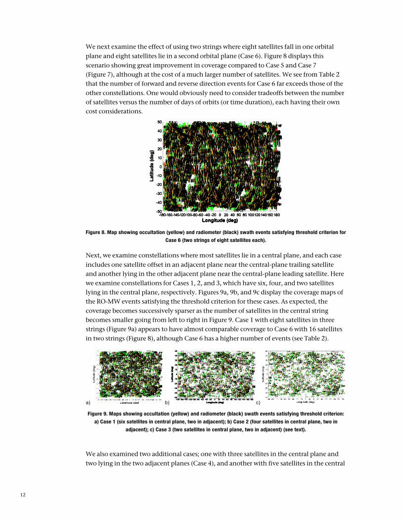
We next examine the effect of using two strings where eight satellites fall in one orbital plane and eight satellites lie in a second orbital plane (Case 6). Figure 8 displays this scenario showing great improvement in coverage compared to Case 5 and Case 7 (Figure 7), although at the cost of a much larger number of satellites. We see from Table 2 that the number of forward and reverse direction events for Case 6 far exceeds those of the other constellations. One would obviously need to consider tradeoffs between the number of satellites versus the number of days of orbits (or time duration), each having their own cost considerations.
Figure 8. Map showing occultation (yellow) and radiometer (black) swath events satisfying threshold criterion for
Case 6 (two strings of eight satellites each).
Next, we examine constellations where most satellites lie in a central plane, and each case includes one satellite offset in an adjacent plane near the central-plane trailing satellite and another lying in the other adjacent plane near the central-plane leading satellite. Here we examine constellations for Cases 1, 2, and 3, which have six, four, and two satellites lying in the central plane, respectively. Figures 9a, 9b, and 9c display the coverage maps of the RO-MW events satisfying the threshold criterion for these cases. As expected, the coverage becomes successively sparser as the number of satellites in the central string becomes smaller going from left to right in Figure 9. Case 1 with eight satellites in three strings (Figure 9a) appears to have almost comparable coverage to Case 6 with 16 satellites in two strings (Figure 8), although Case 6 has a higher number of events (see Table 2).
a) Case 1 (six satellites in central plane, two in adjacent); b) Case 2 (four satellites in central plane, two in
adjacent); c) Case 3 (two satellites in central plane, two in adjacent) (see text).
We also examined two additional cases; one with three satellites in the central plane and two lying in the two adjacent planes (Case 4), and another with five satellites in the central
plane with two satellites lying in one adjacent plane (offset near the trailing and lead satellites), and with a single satellite lying in the other adjacent plane (Case 8). Figure 10a displays the coverage map for Case 4 and Figure 10b displays the coverage map for Case 8. We see that the Case 8 example provides better coverage as expected given that it involves more satellites over a longer orbital arc.
a) b)
Figure 10. a) Case 4 (2/3/2) using GPS over two days and b) Case 8 (2/5/1) using GPS over two days.
If we take Case 8 and extend the duration out to four days, we get the coverage map shown in Figure 11. If we also add additional GNSS constellations to the mix (GPS, Galileo, and GLONASS) over the same four-day period (not shown), the resulting coverage map pretty much fills up the regions of sparser coverage as expected when we have longer orbital durations and with more transmitting GNSS constellations. The multiple GNSS constellation case might require additional RO processing circuitry on board each satellite to accommodate GNSS constellations with different signaling protocols.
Figure 11. Case 8 with four days duration with GPS only.
In evaluating the performance of each RO-MW satellite constellation, we also examine various figures of merit (FOM). One such FOM includes the number of concurrent RO-MW opportunities where an RO event occurs within 5° spatially and within 30 min temporally of an MW event (such as shown in Figure 4). Another FOM involves the average angular separation between satellite velocity vector and projected occultation direction vector
14
(such as shown in Figure 5). Another FOM includes the number of distinct GNSS transmitters involved in each RO event (such as in Figure 6). Figures 4–6 display these quantities over longitude-latitude space within 20°´10° bins. One could also examine these quantities using other bin sizes. Figure 12a displays the number of RO-MW counts in each 20°´10° cell satisfying the 5° threshold over an entire two-day period for Case 1 (also see Figure 4b). Figure 12b shows how this distribution appears if we use smaller 10°´5° bins.
a) b)
Figure 12. (a) Color map superimposed on occultation opportunity counts for each 20°´10° bin from Figure 4b.
(b) Higher resolution color map in 10°´5° bins.
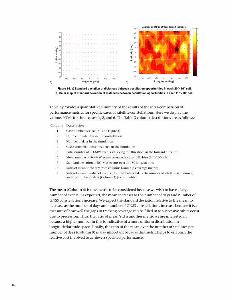
Additional quantities of interest include the average separation between successive occultation centers in each bin shown in Figure 13, and the standard deviation of occultation separation between centers shown in Figure 14. These are calculated as the average of all of the occultation distances in a grouping. A grouping involves a family of occultation swaths having the same transmitter ID. Given that there might be multiple groupings in a cell, it is more difficult to separate the groupings and then calculate this average. Thus, a future study would involve a more comprehensive analysis of average distances between successive occultation events in a grouping.
a) b)
Figure 13. a) Average angular distance between occultation opportunities in each 20°´10° cell; b) Color bar
graph of average angular distances between occultation opportunities in each 20°´10° cell.
Figure 14. a) Standard deviation of distances between occultation opportunities in each 20°´10° cell.
b) Color map of standard deviation of distances between occultation opportunities in each 20°´10° cell.
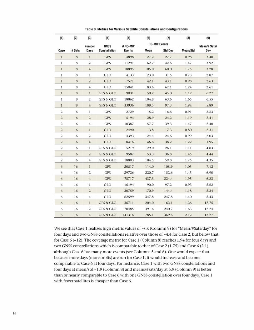
Table 3 provides a quantitative summary of the results of the inter-comparison of performance metrics for specific cases of satellite constellations. Here we display the various FOMs for three cases: 1, 2, and 6. The Table 3 column descriptions are as follows:
Column Description
1 Case number (see Table 2 and Figure 3)
2 Number of satellites in the constellation
3 Number of days in the simulation
4 GNSS constellations considered in the simulation
5 Total number of RO-MW events satisfying the threshold in the forward direction
6 Mean number of RO-MW events averaged over all 180 bins (20°´10° cells)
7 Standard deviation of RO-MW events over all 180 long/lat bins
8 Ratio of mean to std dev from columns 6 and 7 (a coverage metric)
9 Ratio of mean number of events (Column 7) divided by the number of satellites (Column 2) and the number of days (Column 3) (a cost metric)
The mean (Column 6) is one metric to be considered because we wish to have a large number of events. As expected, the mean increases as the number of days and number of GNSS constellations increase. We expect the standard deviation relative to the mean to decrease as the number of days and number of GNSS constellations increase because it is a measure of how well the gaps in tracking coverage can be filled in as successive orbits occur due to precession. Thus, the ratio of mean/std is another metric we are interested in because a higher number in this is indicative of a more uniform distribution in longitude/latitude space. Finally, the ratio of the mean over the number of satellites per number of days (Column 9) is also important because this metric helps to establish the relative cost involved to achieve a specified performance.
16
Table 3. Metrics for Various Satellite Constellations and Configurations
(1) (2) (3) (4) (5) (6) (7) (8) (9)
Case # Sats Number
Days GNSS
Constellation # RO-MW
Events
RO-MW Events
Mean/Std Mean/# Sats/
Day Mean Std Dev
1 8 1 GPS 4898 27.2 27.7 0.98 3.40
1 8 2 GPS 11291 62.7 42.6 1.47 3.92
1 8 4 GPS 18895 105.0 60.0 1.75 3.28
1 8 1 GLO 4133 23.0 31.5 0.73 2.87
1 8 2 GLO 7571 42.1 43.1 0.98 2.63
1 8 4 GLO 15041 83.6 67.1 1.24 2.61
1 8 1 GPS & GLO 9031 50.2 45.0 1.12 6.27
1 8 2 GPS & GLO 18862 104.8 63.6 1.65 6.55
1 8 4 GPS & GLO 33936 188.5 97.3 1.94 5.89
2 6 1 GPS 2729 15.2 16.6 0.91 2.53
2 6 2 GPS 5194 28.9 24.2 1.19 2.41
2 6 4 GPS 10387 57.7 39.3 1.47 2.40
2 6 1 GLO 2490 13.8 17.3 0.80 2.31
2 6 2 GLO 4393 24.4 24.6 0.99 2.03
2 6 4 GLO 8416 46.8 38.2 1.22 1.95
2 6 1 GPS & GLO 5219 29.0 26.1 1.11 4.83
2 6 2 GPS & GLO 9587 53.3 36.8 1.45 4.44
2 6 4 GPS & GLO 18803 104.5 59.8 1.75 4.35
6 16 1 GPS 20517 114.0 108.9 1.05 7.12
6 16 2 GPS 39726 220.7 152.6 1.45 6.90
6 16 4 GPS 78717 437.3 224.4 1.95 6.83
6 16 1 GLO 16194 90.0 97.2 0.93 5.62
6 16 2 GLO 30759 170.9 144.4 1.18 5.34
6 16 4 GLO 62599 347.8 247.8 1.40 5.43
6 16 1 GPS & GLO 36711 204.0 162.1 1.26 12.75
6 16 2 GPS & GLO 70485 391.6 240.7 1.63 12.24
6 16 4 GPS & GLO 141316 785.1 369.6 2.12 12.27
We see that Case 1 realizes high metric values of ~six (Column 9) for “Mean/#Sats/day” for four days and two GNSS constellations relative over those of ~4.4 for Case 2, but below that for Case 6 (~12). The coverage metric for Case 1 (Column 8) reaches 1.94 for four days and two GNSS constellations which is comparable to that of Case 2 (1.75) and Case 6 (2.1), although Case 6 has many more events (see Columns 5 and 6). One would expect that because more days (more orbits) are run for Case 1, it would increase and become comparable to Case 6 at four days. For instance, Case 1 with two GNSS constellations and four days at mean/std ~1.9 (Column 8) and means/#sats/day at 5.9 (Column 9) is better than or nearly comparable to Case 6 with one GNSS constellation over four days. Case 1 with fewer satellites is cheaper than Case 6.
17
The mean/std of 1.75 (Column 8) for Case 1 with GPS only at four days lies below the 1.95 for Case 6 with four days and one GNSS constellation. Thus, Case 6 is comparable to Case 1 at four days and using only the GPS constellation.
The mean number of RO-MW events of 188.5 for Case 1 with four days and two GNSS constellations (Column 6) is comparable (just below) to that of Case 6 with one constellation (GPS) over two days. Thus, we could infer that the Case 1 constellation with two GNSS constellations and four days of orbits is just as cost effective (5.9) as Case 6 with one GNSS over four days (~5–7). Case 1 is obviously better than Case 2 for the metrics with the same number of GNSS constellations and same number of days. Likewise, we see that the mean number of events at 104.5 (Column 6) for Case 2 with four days and two GNSS constellations would be equivalent to Case 1 over two days with two GNSS constellations at 104.8. Again, as one adds more GNSS constellations and more days of observations for a given receiver constellation with fewer satellites (Case 2), it becomes competitive or better with constellations involving more satellites. Thus, one can use such tables to make tradeoffs between the various metrics, which in some cases can serve as figures of merit.
We are assuming that all satellites in a constellation include equipment to allow for performing both RO and MW measurements. These metrics will change as we reduce the number of satellites carrying MW measurement capability, and will change significantly as we run the simulations out to a higher number of days (say, 10) and include more GNSS constellations.
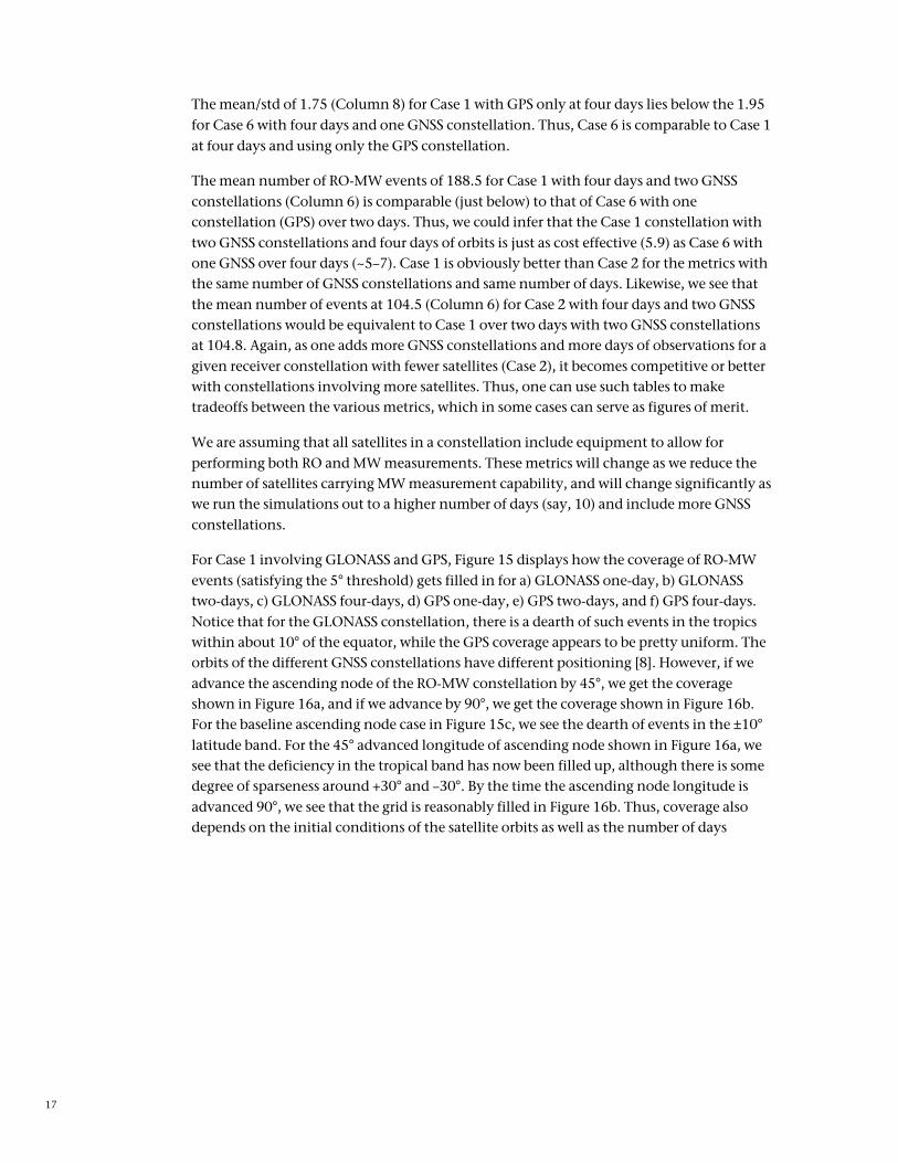
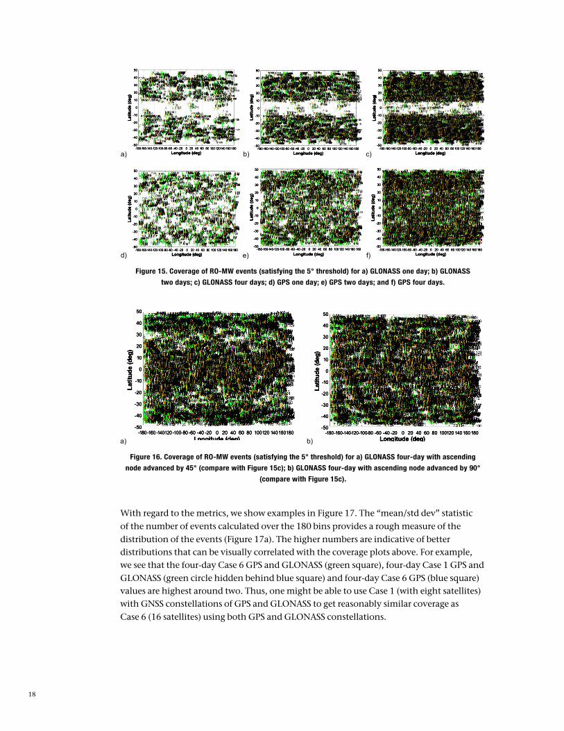
For Case 1 involving GLONASS and GPS, Figure 15 displays how the coverage of RO-MW events (satisfying the 5° threshold) gets filled in for a) GLONASS one-day, b) GLONASS two-days, c) GLONASS four-days, d) GPS one-day, e) GPS two-days, and f) GPS four-days. Notice that for the GLONASS constellation, there is a dearth of such events in the tropics within about 10° of the equator, while the GPS coverage appears to be pretty uniform. The orbits of the different GNSS constellations have different positioning [8]. However, if we advance the ascending node of the RO-MW constellation by 45°, we get the coverage shown in Figure 16a, and if we advance by 90°, we get the coverage shown in Figure 16b. For the baseline ascending node case in Figure 15c, we see the dearth of events in the ±10° latitude band. For the 45° advanced longitude of ascending node shown in Figure 16a, we see that the deficiency in the tropical band has now been filled up, although there is some degree of sparseness around +30° and –30°. By the time the ascending node longitude is advanced 90°, we see that the grid is reasonably filled in Figure 16b. Thus, coverage also depends on the initial conditions of the satellite orbits as well as the number of days
18
a) b) c)
d) e) f)
Figure 15. Coverage of RO-MW events (satisfying the 5° threshold) for a) GLONASS one day; b) GLONASS
two days; c) GLONASS four days; d) GPS one day; e) GPS two days; and f) GPS four days.
a) b)
Figure 16. Coverage of RO-MW events (satisfying the 5° threshold) for a) GLONASS four-day with ascending
node advanced by 45° (compare with Figure 15c); b) GLONASS four-day with ascending node advanced by 90°
(compare with Figure 15c).
With regard to the metrics, we show examples in Figure 17. The “mean/std dev” statistic of the number of events calculated over the 180 bins provides a rough measure of the distribution of the events (Figure 17a). The higher numbers are indicative of better distributions that can be visually correlated with the coverage plots above. For example, we see that the four-day Case 6 GPS and GLONASS (green square), four-day Case 1 GPS and GLONASS (green circle hidden behind blue square) and four-day Case 6 GPS (blue square) values are highest around two. Thus, one might be able to use Case 1 (with eight satellites) with GNSS constellations of GPS and GLONASS to get reasonably similar coverage as Case 6 (16 satellites) using both GPS and GLONASS constellations.
x x x
xx x x
19
a) b)
Figure 17. a) “Mean/St. dev” metric of the number of RO-MW opportunities for the different situations shown in
Table 3; b) Cost metric for the various scenarios shown in Table 3.
Figure 18 displays a side-by-side comparison of the Case 1 constellation (Figure 18a) versus the Case 5 constellation (Figure 18b) for concurrent RO-MW events within 5° threshold for the same 4-day period using only the GPS constellation. SOAP depictions of the two constellations are shown in Figure 2a for Case 1 with two satellites offset in different planes, and Figure 2e for the case of all eight satellites lying in a single plane. The coverage is superior for the eight-satellite case with two satellites offset in different planes (Case 1) versus that of the case for eight satellites all lying in the same plane (Case 5). Thus, this example illustrates the advantage of having some satellites offset in different planes, allowing coverage holes to be more quickly filled up.
a) b)
Figure 18. Side-by-side comparison of coverage for the Case 1 constellation (a) and for the Case 5 constellation
(b) where concurrent RO-MW events lie within a 5° threshold for the same four-day period using the
GPS constellation.
x x
20
VI. Conclusion
We performed simulations involving different constellations (orbit strategies) to assess opportunities where radio occultation events lie within a given threshold relative to nadir-pointed microwave radiometry measurements. We also considered the number of participating GNSS constellations (such as GPS, Galileo, and GLONASS), as well as the number of days for analysis over which the observations are acquired. Based on this analysis, it appears that an eight-satellite constellation consisting of three orbital planes with about six satellites in the central plane and one satellite each in each adjacent plane is reasonably efficient in terms of global coverage and cost. As more days of coverage are realized, a somewhat smaller constellation might suffice. One can make trade-offs based on given receiver constellation configurations, number of days, number of GNSS constellations, and other considerations using the approaches presented in this article.
Acknowledgments
We appreciate the feedback and informative discussions we received during the progress of this task from Tanvir Islam, Kuo-Nung Wang, George Hajj, and Svetla Hristova-Veleva. We also thank Eric Fetzer for the thorough review of this paper.
References
[1] J. Turk, et al., “Benefits of a Closely-Spaced Satellite Constellation of Atmospheric Polarimetric Radio Occultation Measurements,” Remote Sensing, vol. 11, no. 20, p. 2399, 2019.
[2] E. Cardellach, S. Oliveras, A. Rius, S. Tomás, C. O. Ao, G. W. Franklin, B. A. Iijima, D. Kuang, T. K. Meehan, R. Padullés, et al., “Sensing heavy precipitation with GNSS polarimetric radio occultations,” Geophys. Res. Lett., vol. 46, pp. 1024–1031, 2019.
[3] Z. S. Haddad, R. C. Sawaya, S. Kacimi, O. O. Sy, F. J. Turk, and J. Steward, “Interpreting millimeter-wave radiances over tropical convective clouds,” J. Geophys. Res. Atmos., vol. 122, pp. 1650–1664, 2017. doi: 10.1002/2016JD025923.
[4] K.-N. Wang, M. de la Torre Juárez, C. O. Ao, and F. Xie, “Correcting negatively biased refractivity below ducts in GNSS radio occultation: an optimal estimation approach towards improving planetary boundary layer (PBL) characterization,” Atmos. Meas. Tech., vol. 10, pp. 4761–4776, 2017. https://doi.org/10.5194/amt-10-4761-2017.
[5] D. Y. Stodden and G. D. Galasso, “Space system visualization and analysis using the satellite orbit analysis program (SOAP),” Proceedings of the 1995 IEEE Aerospace Applications Conference, Aspen, Colorado, 4–11 February 1995. http://ieeexplore.ieee.org/stamp/stamp.jsp?arnumber=00468892 .
[6] F. J. Wentz, “A 17-yr climate record of environmental parameters derived from the Tropical Rainfall Measuring Mission (TRMM) microwave imager.” J. Climate, vol. 28, pp. 6882–6902, 2015.
[7] J. Turk, D. D. Morabito, C. O. Ao, E. Wang, and M. de la Torre Juarez, “Combining polarimetric radio occultations (PRO) and passive microwave observations to enhance the STORM-PROBE science investigation concept,” Extension to Advanced Concepts Study: Final Report, Jet Propulsion Laboratory, Pasadena, California, 6 October 2020.
[8] X. Li, M. Ge, X. Dai, X. Ren, M. Fritsche, J. Wickert, and H. Schuh, “Accuracy and reliability of multi-GNSS real-time precise positioning: GPS, GLONASS, BeiDou, and Galileo,” J Geod, vol. 89, pp. 607–635, 2015. doi: 10.1007/s00190-015-0802-8. https://link.springer.com/article/10.1007/s00190-015-0802-8 .