Iran Agricultural Research An evaluation of genetic...

Iran Agricultural Research (2017) 36(1) 91-104

An evaluation of genetic algorithm method compared to geostatistical and neural network methods to estimate saturated soil hydraulic conductivity using soil texture Y. Hoseini1*, R. Sedghi2, S. Bairami2

1Moghan College of Agriculture and Natural Resources, University of Mohaghegh Ardabili, Ardabil, I. R. Iran 2Sama Technical and Vocatinal Training College, Islamic Azad University, Ardabil Branch, Ardabil, I. R. Iran

* Corresponding Author: [email protected]

ARTICLE INFO

ABSTRACT-Determining hydraulic conductivity of soil is difficult, expensive, and time-consuming. In this study, genetic algorithm (GA) and geostatistical analysis and Neural Network method are used to estimate soil saturated hydraulic conductivity using the properties of particle size distribution. The data were gathered from 134 soil profiles from soil and lander form studies of the Ardabil Agricultural Organization. Results showed that Ordinary cokriging has the best fit for the geostatistical methods. The best-fitted variogram was the exponential model with a nugget effect of 0 cm day-1 and sill of 156 cm day-1 which is the strength of the spatial structure and full effect of the structural components on the variogram model for the region; also, in the ordenary cokriging method, an accurate estimate was obtained using R2 = 0.93 and RMSE = 3.21.Multilayer perceptron (MLP) network used the Levenberg- Marquardt (trainlm) algorithm with are a regression coefficient of 0.997 and RMSE of 1.22 to estimate the hydraulic conductivity of saturated soil. For GA model, parameters and R2 were determined as 1.35 and 0.926 cm day-1 respectively. Performance evaluation of the models showed that the Neural Network model compared with geostatistical analysis and genetic algorithm was able to predict soil hydraulic conductivity with high and more accuracy and results of this method was closer to the measurement results.

Article history:Received 17 January 2016 Accepted 4 March 2017 Available online 5 April 2017

Keywords:Geostatistics Saturated hydraulic conductivity Neural Network Methods (ANN) Cokriging Genetic algorithm

INTRODUCTION

Measuring properties such as hydraulic conductivity of saturated soil is most important for the technical and economic aspects of the design of drainage projects. Measurement of these properties is often difficult because they are costly, time-consuming and result in high spatial and temporal variability. Soft computing techniques such as Artificial Neural Networks, fuzzy inference systems, evolutionary computation, and their hybrids have been successfully employed to develop predictive models to estimate parameters. These techniques are attractive because they tolerate a wide range of uncertainty. Soft computing techniques are now used as alternate statistical tools. Geostatistical and neural networks methods can estimate soil parameters such as hydraulic conductivity with reasonable accuracy. Geostatistic methods are more efficient than classic estimation methods based on random variables because classic methods do not consider data location

and direction when estimating random variable sat the regional level. However, geostatistical estimation takes these two factors in to consideration. Geostatistics can also calculate estimation error and sampling error, carry out data preparation and offer an index for estimating the strength of spatial structure and data. Also, the use of soil texture to quickly determine soil parameters using neural networks is a new method of determining the saturated hydraulic conductivity of soil. Neural networks can be used form ode ling for Modeling and extraction of pedestrian’s ferfunctions. An Artificial Neural Network (ANNs) is the most widespread of intelligent systems, has a mathematical structure, and can processor betray linear combinations to communicate between the inputs and outputs of the system. Fig. 1. is a simple model of an ANN. A typical network consists of the input, mean layer (hidden), and output layer.

Shiraz University

Hoseini and Sedghi / Iran Agricultural Research (2017) 36(1) 91-104

92

Fig. 1. Structure of ANN

Delbari et al. (2004) used 605 measured hydraulic

conductivity data to assess geostatistical methods in terms of estimating soil hydraulic conductivity in the slope areas of the water and behind the water of the down part of Sis tan Plain. In this study, the applied interpolation methods included cokriging, a weighted moving average, and TPSS. To compare statistical criteria of the methods, mean absolute error was applied. In this work, hydraulic conductivity was measured in both saturated and unsaturated methods and the data of both methods were separately studied. Findings showed that hydraulic conductivity did not have high spatial correlations in Sistan region. As a result, cokriging method did not offer reasonable accuracy in the hydraulic conductivity estimation in the mentioned region. The results also showed that for both saturated hydraulic conductivity and unsaturated hydraulic conductivity, TPSS method with the powers (exponential) of 2 and 3 had a better estimation. BegayHerchgani and Heshmati (2012) examined Shahrekord's groundwater quality using geostatistics in irrigation systems. In this study, electrical conductivity (EC), total dissolved salts (TDS), total suspended solids (TSS), and water pH were measured in 97 wells. Also, ordinary cokriging method was used for zoning the variables and RMSE criterion was applied for demonstrating the accuracy of the estimations. In all the indicators, less than 40% was obtained that indicated the estimated accuracy was good. Nezami and Alipour (2012) provided soil salinity map using geostatistical methods in Qazvin Plain. Based on the ground assessments, soil salinity was a limiting factor for growing plants; so, samples were taken from 0 to 30 cm of soil depth in Qazvin plain and electrical conductivity (EC), pH, and percentage of the samples were measured. In this study, several methods including cokriging, Spline, and inverse distance weighting were used to assess soil salinity. The researchers found that use of auxiliary variables such as height and soil texture which have high correlation with the main variables increased the accuracy of the interpolation method. As a result, in this study, cokriging method using clay percentage as a covariate had high accuracy in anticipation. Hoseini (2004) optimized the estimation of hydraulic conductivity using cokriging method. In this study that was conducted for fulfilling the requirement for a Master's degree, it was tried to do region-rated agricultural land in the Weiss in terms of hydraulic conductivity using geostatistics. Also, isolated areas were compared in terms of hydraulic conductivity (low, medium, and high) using Thiess

Polygon-rated method. The results showed that cokriging method area with low hydraulic conductivity and average expend rather than Thiess and also on the high hydraulic conductivity of area by Thiess was more than cokriging that This makes with considering the amount of hydraulic conductivity more than the actual in these areas with thiess method. Obtained draining distances in these areas are less than the actual amount. Merdun et al. (2006) used transfer functions and neural networks to estimate the saturated hydraulic conductivity. In this study, 130 data samples for the creation of models and the remaining 65 samples were used to evaluate the models. The results showed that regression models had better estimates of saturated hydraulic conductivity than Artificial Neural Networks. However, the mentioned differences were not statistically significant for the estimation of the considered variables. Navabian et al. (2004) applied Artificial Neural Network by using soil quickly finding parameters which modeled the saturated hydraulic conductivity. They introduced bulk density, effective porosity, geometric mean of particle size and geometric standard deviation of particle size as critical parameters. Doaie et al. (2005) estimated the saturated hydraulic conductivity using 221 soil samples from Guilan Province and measuring parameters of organic carbon, sand, silt, clay, bulk density, and saturated hydraulic conductivity. In the present study, three different models were used: Model (1) included the parameters of sand, silt, and clay; Model (2) included the parameters for clay content, bulk density, and organic matter; and Model (3) included the parameters of organic matter, sand, silt, clay, and bulk density. Comparison of the obtained results showed that although neural networks could offer an acceptable estimation of soil hydraulic conductivity using all the three models, the input model had high accuracy and less error in the estimation of saturated hydraulic conductivity compared to others. So, due to the limited number of similar studies conducted inside and outside the country and considering the difficulty, time consumption, and measuring cost of the direct method, the purpose of this study was to estimate the saturated hydraulic conductivity. For this purpose, some parameters of soil which are quickly found such as the percentage of clay particles, silt, and sand were measured using Artificial Neural Network techniques and methods based on geostatistics; then, the accuracy of these methods was compared. Cadenas and Rivera (2009) predicted wind speed in the areas of Lavnta, Osaka, and Mexico using Artificial Neural Network model for a short term. Their results showed that a


93

three-layer preceptor model with 7 Nero on the hidden layer had the best performance so that the error square mean and its absolute mean were 0.0016 and 0.0399, respectively, showing the high accuracy of the designed network. Dahamsheh and Aksoy (2009) used feed-forward Artificial Neural Networks and predicted the next month rainfall in three stations using different climatic conditions. The results were compared with those of a multivariate regression model and it was concluded that, for humid climate stations, Artificial Neural Networks and multivariate regression model were more suitable for drier areas. So, the aim of this study was to compare two methods for determining hydraulic conductivity of soil using geostatistical methods and Artificial Neural Networks and assess the accuracy of each of them. Results of studies done by Kim and Kim (2008) and Kayadelen (2011) have shown that by optimizing input parameters and selecting the number of middle layer in Fuzzy Inference Systems and Genetic Algorithm accurately, the results of these two methods will be optimized. The results of Haghverdi et al. (2011) demonstrated the superior performance of Genetic Neural Algorithm than Fuzzy Neural Algorithm on characteristic curve of soil moisture. (Prasad and Mathur, 2007). Neural Network Method is used to estimate the accuracy of genetic algorithm when measurement data lack high accuracy.

There has been a limited number of published studies and the direct methods have drawbacks such as level of difficulty, time-consumption, and cost of measurement. The present study estimated the saturated hydraulic conductivity using soil parameters that are quickly found, such as percentage of clay particles, silt, and sand using ANNs, geostatistics and GA methods and compared the accuracy of these methods.

MATERIALS AND METHODS The studied region with the area of 5181. 89 ha was located on a piece of land in Fathali Plain at the distance of approximately 35 km southwest of Parsabad City and

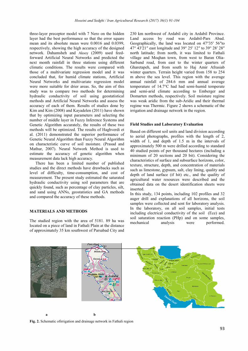
230 km northwest of Ardabil city in Ardabil Province. Land access by road was Ardabil-Pars Abad. Geographically, the land was located on 47°35′ 56″to 47° 43′21″ east longitude and 39° 25′ 12″ to 39° 28′ 28″north latitude; from north, it was limited to Fathali village and Moqhan town, from west to Baran Olia-Sarband road, from east to the winter quarters of Gharetapeh, and from south to Haj Amir Afrasiab winter quarters. Terrain height varied from 158 to 254 m above the sea level. This region with the average annual rainfall of 284.6 mm and annual average temperature of 14.7°C had had semi-humid temperate and semi-arid climate according to Emberger and Domarten methods, respectively. Soil moisture regime was weak aridic from the sub-Aridic and their thermal regime was Thermic. Figure 2 shows a schematic of the irrigation and drainage network in the region.

Field Studies and Laboratory Evaluation

Based on different soil units and land division according to aerial photographs, profiles with the length of 2, width of 1, and depth of 1.5 m in the intervals of approximately 500 m were drilled according to standard 40 studied points of per thousand hectares (including a minimum of 20 sections and 20 bit). Considering the characteristics of surface and subsurface horizons, color, texture, structure, depth, and concentration of materials such as limestone, gypsum, salt, clay lining, quality and depth of land surface (if hit) etc., and the quality of agricultural water resources were described and the obtained data on the desert identification sheets were inserted. In this study, 134 points, including 102 profiles and 32 auger drill and explanations of all horizons, the soil samples were collected and sent for laboratory analysis. In the laboratory, on all soil samples, initial tests including electrical conductivity of the soil (Ece) and soil saturation reaction (PHp) and on some samples, mechanical analysis were performed.

a b

Fig. 2. Schematic ofirrigation and drainage network in Fathali region


94

soils and land use classification was determined based on interpreting aerial photographs information, profiles description, drills and the primary chemical experiments on normal effects with a scale of 1:5000. According to the soil properties and considering the characteristics of each profile, complete chemical analysis of soils and soil series was performed. To measure physical parameters, different depths of undisturbed samples were prepared and the required parameters were determined in the laboratory. Physical and chemical properties of studied soil are shown in Table 1. Neural Network Model

Neural networks can be used as a direct substitute for auto correlation, multivariable regression, linear regression, trigonometric, and other statistical analysis and techniques. Neural networks, with their remarkable ability to derive a general solution from complicated or imprecise data, can be used to extract patterns and detect trends that are too complex to be noticed by either humans or other computer techniques. A trained neural network can be thought of as an ‘‘expert’’ in the category of information it has been given to analyze. This expert can then be used to provide projections given new situations of interest and answer ‘‘what if’’ questions. When a data stream is analyzed using a neural network, it is possible to detect important predictive patterns that are not previously apparent to a non-expert. Thus, the neural network can act as an expert. The particular network can be defined by three fundamental components: transfer function, network architecture, and learning law. It is essential to define these components, to solve the problem satisfactorily. In this study, the architectures of ANN- multi-layer preceptor (MLP) were also used to estimate the soil saturated hydraulic conductivity using soil texture. MLP network models are the popular network architectures used in most research applications in medicine, engineering, and mathematical modeling. In MLP, the weighted sum of the inputs and bias term are passed to the activation level through a transfer function to produce the output, and the units are arranged in a layered feed-forward neural network (Venkatesan and Anitha, 2006). Before training the neural network, the input data were normalized. The purpose of normalization was to transform data into numbers between zero and one. In this study, for processing elements (neurons-S) in the hidden layer, the sigmoid threshold function selected as the output of this function should be numbers between 0 to 1; thus, the input function of data should be numbers between zero and one. For inputs close to zero and one, the changes of neuron weight would be minimal, because on this number, processor components would act slowly due to the sigmoid function; but, for the input values close to the half, the response of the neurons to the input signals would be faster. Considering this issue, the data-normalization was done in such a way that the mean of

the data set was 0.5. For this purpose, the following equation was used for the normalization.

_

0

max min

0.5( ) .5Xnorm oX XX X

−= +

−(1)

where Xnorm is the normalized input of X0, X� is the mean of data, and Xmax and Xmin are the maximum and minimum pieces of data, respectively.

All data were divided into training (50% of all data), testing (25% of all data) and verification (25% of all data) sets. Matlab 7.2 software was used in neural network analyses having a three-layer feed-forward network consisting of an input layer (3 neurons), one hidden layer (11 neurons) and one output layer. The number of neurons in the hidden layers was selected after a series of trial runs of networks having 1 to 20 neurons to obtain the neuron number in the network having minimum error. Network parameters of learning rate and momentum were set at 0.01 and 0.9, respectively. The variable learning rates were used for all layers with momentum as the network training function and tan-sigmoid (tansig) as an activation (transfer) function. Geostatistical Analysis

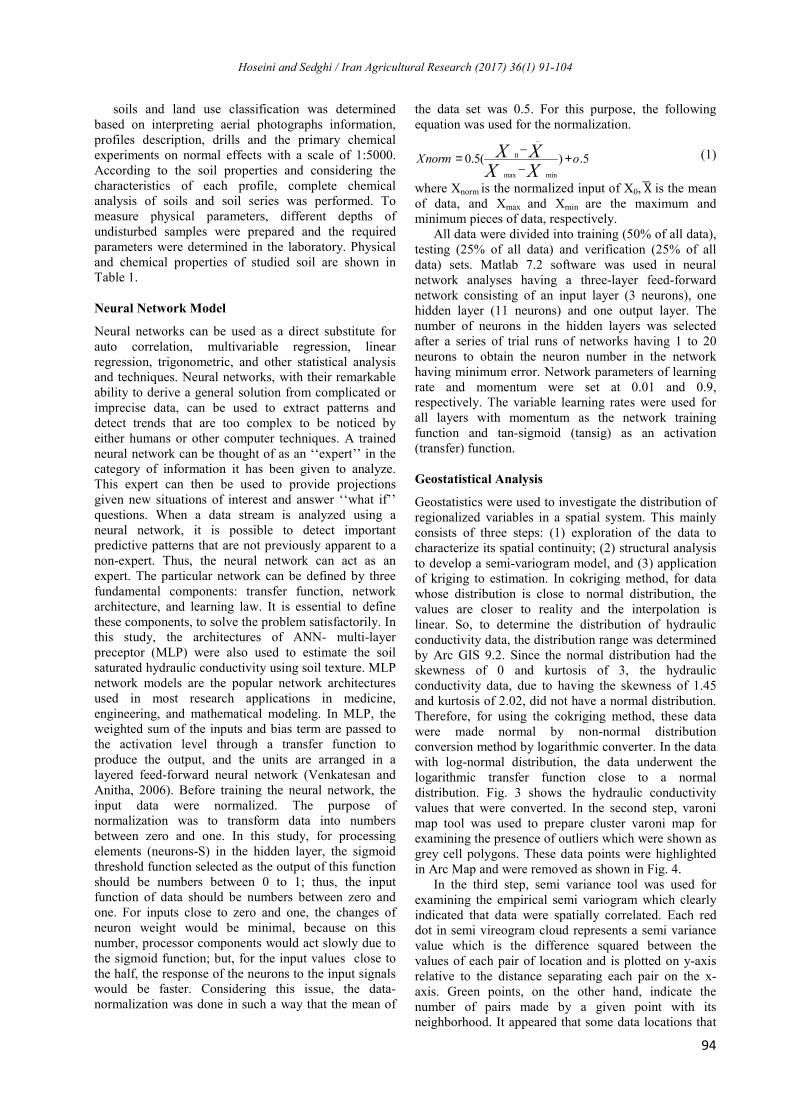
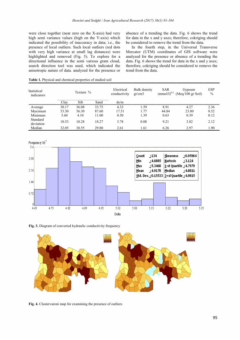
Geostatistics were used to investigate the distribution of regionalized variables in a spatial system. This mainly consists of three steps: (1) exploration of the data to characterize its spatial continuity; (2) structural analysis to develop a semi-variogram model, and (3) application of kriging to estimation. In cokriging method, for data whose distribution is close to normal distribution, the values are closer to reality and the interpolation is linear. So, to determine the distribution of hydraulic conductivity data, the distribution range was determined by Arc GIS 9.2. Since the normal distribution had the skewness of 0 and kurtosis of 3, the hydraulic conductivity data, due to having the skewness of 1.45 and kurtosis of 2.02, did not have a normal distribution. Therefore, for using the cokriging method, these data were made normal by non-normal distribution conversion method by logarithmic converter. In the data with log-normal distribution, the data underwent the logarithmic transfer function close to a normal distribution. Fig. 3 shows the hydraulic conductivity values that were converted. In the second step, varoni map tool was used to prepare cluster varoni map for examining the presence of outliers which were shown as grey cell polygons. These data points were highlighted in Arc Map and were removed as shown in Fig. 4.

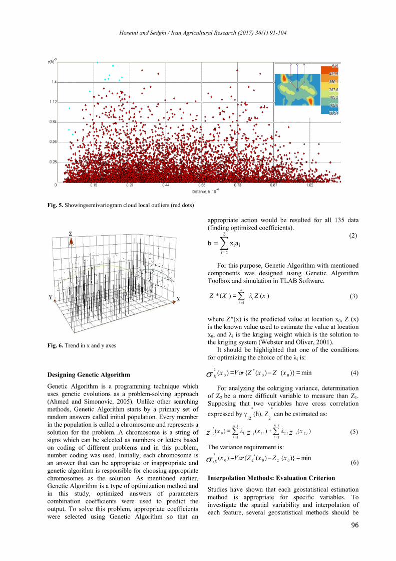
In the third step, semi variance tool was used for examining the empirical semi variogram which clearly indicated that data were spatially correlated. Each red dot in semi vireogram cloud represents a semi variance value which is the difference squared between the values of each pair of location and is plotted on y-axis relative to the distance separating each pair on the x-axis. Green points, on the other hand, indicate the number of pairs made by a given point with its neighborhood. It appeared that some data locations that


95

were close together (near zero on the X-axis) had very high semi variance values (high on the Y-axis) which indicated the possibility of inaccuracy in data; i.e., the presence of local outliers. Such local outliers (red dots with very high variance at small lag distances) were highlighted and removed (Fig. 5). To explore for a directional influence in the semi various gram cloud, search direction tool was used, which indicated the anisotropic nature of data. analyzed for the presence or

absence of a trending the data. Fig. 6 shows the trend for data in the x and y axes; therefore, cokriging should be considered to remove the trend from the data.

In the fourth step, in the Universal Transverse Mercator (UTM) coordinates of GIS software were analyzed for the presence or absence of a trending the data. Fig. 6 shows the trend for data in the x and y axes; therefore, cokriging should be considered to remove the trend from the data.

Table 1. Physical and chemical properties of studied soil

Statistical indicators

Texture % Electrical

conductivity

Bulk density gr/cm3

SAR (mmol/l)0.5

Gypsum (Meq/100 gr Soil)

ESP %

Clay Silt Sand ds/m Average 30.17 36.08 33.75 4.33 1.59 8.91 4.27 2.36 Maximum 53.30 56.30 87.60 17.51 1.77 44.84 23.80 8.52 Minimum 5.60 4.10 11.00 0.50 1.39 0.63 0.39 0.12 Standard deviation 10.53 10.28 18.27 3.78 0.08 9.21 3.82 2.12

Median 32.05 38.55 29.80 2.61 1.61 6.26 2.97 1.90

Fig. 3. Diagram of converted hydraulic conductivity frequency

Fig. 4. Clustervaroni map for examining the presence of outliers


96

Fig. 5. Showingsemivariogram cloud local outliers (red dots)

Fig. 6. Trend in x and y axes

Designing Genetic Algorithm

Genetic Algorithm is a programming technique which uses genetic evolutions as a problem-solving approach (Ahmed and Simonovic, 2005). Unlike other searching methods, Genetic Algorithm starts by a primary set of random answers called initial population. Every member in the population is called a chromosome and represents a solution for the problem. A chromosome is a string of signs which can be selected as numbers or letters based on coding of different problems and in this problem, number coding was used. Initially, each chromosome is an answer that can be appropriate or inappropriate and genetic algorithm is responsible for choosing appropriate chromosomes as the solution. As mentioned earlier, Genetic Algorithm is a type of optimization method and in this study, optimized answers of parameters combination coefficients were used to predict the output. To solve this problem, appropriate coefficients were selected using Genetic Algorithm so that an

appropriate action would be resulted for all 135 data (finding optimized coefficients).

(2) � ��

�

��

For this purpose, Genetic Algorithm with mentioned components was designed using Genetic Algorithm Toolbox and simulation in TLAB Software.

(3)

where Z*(x) is the predicted value at location x0, Z (x) is the known value used to estimate the value at location x0, and λi is the kriging weight which is the solution to the kriging system (Webster and Oliver, 2001).

It should be highlighted that one of the conditions for optimizing the choice of the λi is:

(4)

For analyzing the cokriging variance, determination

of Z2 be a more difficult variable to measure than Z1.Supposing that two variables have cross correlation expressed by γ

12

*(h), Z

2

*can be estimated as:

(5)

The variance requirement is:

(6)

Interpolation Methods: Evaluation Criterion

Studies have shown that each geostatistical estimation method is appropriate for specific variables. To investigate the spatial variability and interpolation of each feature, several geostatistical methods should be

1

* ( ) ( )n

ii

Z X Z xλ=

=∑

2 *0 0 0( ) { ( ) ( )} minK x Var Z x Z xσ = − =

2 *0 2 0 2 0( ) { ( ) ( )} mincK x Var Z x Z xσ = − =

1 2*

0 1 1 2 22 1 21 1

( ) ( ) ( )N N

i i j ji i

x x xz z zλ λ= =

= +∑ ∑


97

compared and evaluated and the best one chosen depending on the desirable accuracy and ease of use. The comparison technique used here was the mutual authentication method where each time an observation point was removed from adjacent points, a value is estimated. The actual value returns to the previous location and, for all grid points, this operation is repeated. Finally, given the observed and estimated values, the percentage of relative errs or (ε), Average Amount of Error (MAE), and RMSE of each method is calculated as:

(7)

(8)

(9)

in which )(*

ixZ . The estimated amount at xi points is )( ixZThe observed value is at point xi, N is the number of points, MAE represents the accuracy and average amount of error (whichever is closer to zero is better). The value of ε represents the estimated me and eviction of the observed value (whichever the lower is better). In practice, the revalues will not be zero. Theoretically, when the two values are equal to zero, the accuracy is 100% and the estimated value is exactly equal to the actual value.

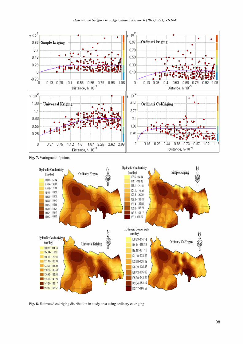
RESULTS AND DISCUSSION Predicting Saturated Hydraulic Conductivity Using Geo-Statistical Method By plotting the directional variogram assuming the non-uniform region in the directions 0°, 45°, 90° and 135°, it can be seen that these variograms were homogeneous in different directions and had the same type and the effecting range and sill effects are the same and follow homogeneity of the spatial structure of the model, on these exponential variograms models, the nugget effect is (0.002 mm day-1) and the maximum sill (0.006 mm day-1). Considering these numbers, due to the nugget effect to the sill of smaller than 0.5 (C0/Q2<0.5), it can be concluded that the role of structured component of the variogram was greater than that of the non-structured component. This issue showed the strength of the spatial structure of the region. Then, different combinations of kriging (ordinary, simple and universal) were taken and their cross validation statistics were compared (Fig. 9). It was observed that for all types of kriging, predictions were unbiased as mean of prediction errors was nearer to zero (0.05 - 0.1) and prediction of standard errors was appropriate as indicated by the closeness of the root-mean-square prediction error and average standard prediction error values (differences in their magnitude were 1.68 - 3). But predictions were not close to measured values as

indicated by appreciable magnitude of root-mean-square prediction error (nearly 1.5) and also best fit line was far away from 1:1 line and slope of best fit line was less (0.51). The results thus described these choices as not desirable. In the next step, soil physical parameters such as sand and soil clay were used to help the estimation; for this work, cokriging method was used. The best fitted variogram in this way was exponential variogram model with the nugget effect of 0 mm day-1 and sill of 156 mm day-1 that represented the strength of the spatial structure of the region and the full impact of structured component on variogram model for the region.

Also, the obtained variogram can show spatial correlation data to the range of 1998 m; this amount can be used in the sampling grid reduction to estimate the saturated hydraulic conductivity in the area. As a result, using the measurements, a limited number of hydraulic conductivity, and soil texture in the area and using cokriging algorithm, hydraulic conductivity can be estimated in the whole area with good accuracy (Merdun et al., 2006). Fig. 7 shows the resulting variogram. In Fig. 8, distribution of estimation in the area for ordinary cokriging is shown. To evaluate whether or not the obtained estimates were biased, cross-validation method was used as can be seen in Fig. 9. The estimated value for ordinary cokriging was very close to the measured values, which led the fitted line between the actual and estimated values to be close to the angle of 45°. As shown in the evaluation of the mentioned method, using the soil quickly finding parameters such as sand and clay and silt, rate of the conducted estimates in the area can be performed with very high precision; so, the slope of the fitted line was close to value 1.

As the results show, it is evident that the geostatistical methods are dependent to soil characteristics to accurately estimate saturated soil hydraulic conductive it yap plying cokriging without the use of auxiliary variables. In the hydraulic conductivity, estimation did not have accurate results. One of the reasons could be the inaccuracy of using block cokriging method, instead of point cokriging (Basaran et al., 2011; Kaplana and Agval, 2011); but, considering soil texture as the effective parameter in the hydraulic conductivity, estimation is very close to the true value. One of the advantages of geostatistics over other estimation methods such as neural networks is that hydraulic conductivity estimation can be noted in all areas in which measurements are done. In fact, using this method, hydraulic conductivity map is provided at the regional level that can be directly used on irrigation and drainage networks with high confidence. Hosseini et al. (1993) investigated the spatial variability of soil hydraulic conductivity in the southwest of Iran and concluded that in this area, soil hydraulic conductivity had moderate spatial correlation by comparing the piece effect to the threshold which is over 60 percent.

∑=

−=n

iniii xZxZxZ

1

* /100*)(/)()(ε

∑=

−=n

inii xZxZMAE

1

* /))()((

∑=

−=n

iii nxZxZRMSE

1

21

/2* ))()((


98

Fig. 7. Variogram of points

Fig. 8. Estimated cokriging distribution in study area using ordinary cokriging


99

Fig. 9. Evaluation of cross-validation method for ordinary cokriging

However, Alemi et al. (1980) studied the spatial variability of hydraulic conductivity and reported the presence of spatial dependence in this field. The results showed that, regardless of variables, space communication among hydraulic conductivity values was low and the obtained variogram had less strength than when the auxiliary variables were used. Even in the latter case, the nugget effect was reduced to zero. Therefore, it can be concluded that the use of auxiliary variables that could directly affect the main variables can specify the spatial structure of the variable region more carefully at the regional level.

Saturated Hydraulic Conductivity Prediction Using ANNs

To find the optimal threshold for networks, different functions including logarithmic sigmoid function, hyperbolic tangent sigmoid, and linear functions were used and, to optimize the weights of percept Ron

networks, the Levenberg–Marco algorithm was used. For each network (ANN), originally, a combination of default and various iterations, values of determination coefficient (R2), and error (RMSE) were studied. After determining the number of layers, number of neurons, threshold functions, and a learning algorithm to train the network, final weights of the neurons were determined. For learning the MLP neural network, the Levenberg-Marco algorithm was used and finally the trial-and-error method was applied to determine the best architecture for this network. Optimal selective architecture for this network had 3 neurons in the input layer, 11 neurons in the hidden layer using tangent sigmoid threshold function, and an output layer of neurons with linear threshold function and 1000 iterations. In all the networks, the learning rate and momentum were equal to 3.0. The regression graphs represent the relationship between measured and predicted values of the ANN with one hidden layer, in the training, validation and test


100

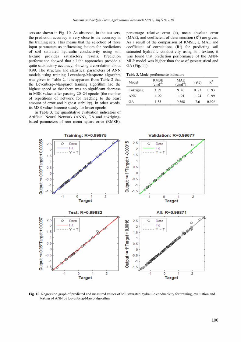
sets are shown in Fig. 10. As observed, in the test sets, the prediction accuracy is very close to the accuracy in the training sets. This means that the selection of three input parameters as influencing factors for predictions of soil saturated hydraulic conductivity using soil texture provides satisfactory results. Prediction performance showed that all the approaches provide a quite satisfactory accuracy, showing a correlation about 0.99. The structure and statistical parameters of ANN models using training Levenberg-Marquette algorithm was given in Table 2. It is apparent from Table 2 that the Levenberg–Marquardt training algorithm had the highest speed so that there was no significant decrease in MSE values after passing 20–24 epochs (the number of repetitions of network for reaching to the least amount of error and highest stability). In other words, its MSE values become steady for lower epochs.

In Table 3, the quantitative evaluation indicators of Artificial Neural Network (ANN), GA and cokriging-based parameters of root mean square error (RMSE),

percentage relative error (ε), mean absolute error (MAE), and coefficient of determination (R2) are given. As a result of the comparison of RMSE, ε, MAE and coefficient of correlations (R2) for predicting soil saturated hydraulic conductivity using soil texture, it was found that prediction performance of the ANN-MLP model was higher than those of geostatistical and GA (Fig. 11).

Table 3. Model performance indicators

Model RMSE (cmd-1)

MAE (cmd-1) ε (%) R2

Cokriging 3. 21 9. 43 0. 23 0. 93 ANN 1. 22 1. 21 1. 24 0. 99 GA 1.35 0.568 7.6 0.926

Fig. 10. Regression graph of predicted and measured values of soil saturated hydraulic conductivity for training, evaluation and testing of ANN by Levenberg-Marco algorithm


101

Table 2. Quantitative indicators of network assessment by Levenberg-Marquette algorithm

Average accuracy Simulation (%)

Correlation coefficient of network Statistically parameters of network Network parameters Number

of neurons Testing Assessment Training R2 RMSE(cmd-1) MomentumConstant learning rate

99.74 0.998 0.996 0.999 0.997 1.22 0.3 0.3 11

In order to predict the soil saturated hydraulic conductivity using soil texture, ANN models (MLP, having three inputs and one output) was applied successfully, and exhibited more reliable predictions than the geostatistical and GA models. The performance comparison showed that the soft computing system is a good tool for minimizing the uncertainties in the soil saturated hydraulic projects. The use of soft computing may also provide new approaches and methodologies, and minimize the potential inconsistency of correlations. Also, the intelligent data analysis methods and the need for additional tests can be considered as a neural network. As is known, the potential benefits of soft computing models extend beyond the high computation rates. Higher performances of the soft computing models were sourced from greater degree of robustness and fault tolerance than traditional statistical models because there are many more processing neurons, each with primarily local connections.

Fig. 12 shows deviation between measured values and the values predicted by models. According to this figure, deviation of values predicted by cokriging model (-0.08876 to +0.11823 for saturated hydraulic soil) is much smaller than the deviation of values predicted by

ANN model (-0.0180 to +0.02756) and GA (-0.0394 to +0.047) for saturated hydraulic soil.

According to the Neural Network Model used in this study, results of this study are not consistent with the results of Salazar et al. (2008) who estimated saturated hydraulic conductivity using Rosetta Model. In their study, the value of saturated hydraulic conductivity using Rosetta Model with neural network nature is 15 percent less than actual values. Although the results of Genetic Algorithms than Artificial Neural Network and ANFIS Model is less accurate, given the obtained correlation coefficient (0.92) and root mean square error (0.35), high accuracy of this method for determining soil hydraulic conductivity is approved. The results provided by Azizpour et al. (2012) and Golshadfasih et al. (2014) on application of genetic algorithm as an optimizer function to estimate the saturated hydraulic conductivity in drainage systems are consistent with the results of this study. Therefore, researchers suggested Genetic Algorithm as an accurate and efficient tool to determine the saturated hydraulic conductivity of soil.

Fig. 11. Comparison of predicted values of cokriging and ANN with measured values

110

120

130

140

150

160

170

1 5 9 13 17 21 25 29 33 37 41 45 49 53 57 61 65 69 73 77 81 85 89 93 97 101

105

109

113

117

121

125

129

133

hydr

aulic

codu

ctiv

ity(C

m/d

ay)

points

Measured (Cokriging) ANN GA


102

Fig. 12. Deviation between measured values and the values predicted by models (COKRIG, ANN,GA)

CONCLUSIONS Hydraulic conductivity is one of the hydrodynamic characteristics of soil that has a determining role in moving and transferring water and soil dissolution. In a drainage project, some soil saturated hydraulic conductivity is necessary. In this study, saturated hydraulic conductivity of soil in Ardabil was predicted using Artificial Neural Network (ANN), geostatistical and genetic algorithm. The results showed that all methods had high accuracy in determining the amount of saturated hydraulic conductivity of soil.

However, Artificial Neural Network had higher accuracy than ordinary cokriging and GA methods and can well simulate saturated hydraulic conductivity of soil with high accuracy and less error. Also, providing good results by Artificial Neural Network (ANN) requires being careful while selecting network components and also selecting a high number of the appropriate constituting elements of the network.

REFERENCES Ahmed, S., & Simonovic, S.P. (2005). An Artificial Neural

Network model for generating hydrograph from hydro meteorological parameters .Journal of Hydrology, 315, 236-251.

Alemi, M.H., Azari, A.S., & Nielsen, D.R. (1980). Krigingand univariate modeling of a spatial correlateddata. Soil Technology, 1, 133-147.

Azizpour, S., Fathi, P., & Nobakhtvakili, K. (2012). Estimating saturated hydraulic conductivity and porosity coupled with intelligent inverse problem approach. Journal of Science and Technology of Agriculture and Natural Resources, Soil and Water Sciences, 60, 13-22. (In Persian).

Basaran, M., Erpul, G., Ozcan, A.U., Saigon, D.S., Kibar, M., Bayramin, I., & Yilman, F.E. (2011). Spatial information of soil hydraulic conductivity and performance of cokriging over kriging in a semi-arid basin scale. Environmental Earth Sciences, 63, 827–838.

BegayHerchgan, H., Heshmati, S.S. (2012). In dicators of ground water quality zoning of Shahrekord’s for using on irrigation system design. Agriculture Water Reourcess., 51, 24-61. (In Persian).

Cadenas, E., & Rivera, W. (2009). Short term wind speed forecasting in La Venta, Oaxaca, Me´xico, using Artificial Neural Networks. Renewable Energy, 34, 274–278.

Dahamsheh, A., & Aksoy, H. (2009). Artificial Neural Network models for forecasting inter mittent monthly precipitation in arid regions. Meteorological Applications, 16, 325-337.

Delbari, M., Tailor mood, M., & Mahdian, M.H. (2004). Evaluation of methods for estimating the hydraulic conductivity of the soil in areas of steep terrain and the bottom surface water of the Sistan plain water. Journal of Agricultural Science,5, 1-12. (In Persian).

Doaie, M., Shabanpour, M., & Bagheri, F. (2005). Modeling of saturated hydraulic conductivity of Gilan Province involving Artificial Neural Networks. The agricultural Science Research Report. Faculty of Agriculture, GilanUnivesity. (In Persian).

Golshadfasih, M., Hooshmand, A.A., & Mehdinezhadiani, B. (2014). Application of genetic algorithms for estimating the saturated soil hydraulic parameters. Journal of Soil Research (Soil and Water Sciences). 28(1), 144-151. (In Persian).

Haghverdi, A., Ghahreman, B., Jalini, M., Khoshnudyazdi, A.A., & Arabi, Z. (2011). Comparison of different methods of artificial intelligence modeling of soil moisture characteristic curve in North and North East of Iran. Research Journal of soil and water conservation methods,18(2), 65-84. (In Persian).

Hoseini, Y. (2004). Drainag parameters optimization using geostatistical methods (Cokriging) and their impact ondrain spacing. Faculty of Water Science Engineering, Chamran University. (In Persian).

Hosseini, E., Gallich and, J, & Caren, J. (1993). Comparison of several in terpol ators for smoothing hydrauliccond

-0.04

-0.03

-0.02

-0.01

0

0.01

0.02

0.03

0.04

0.05

1 6 11 16 21 26 31 36 41 46 51 56 61 66 71 76 81 86 91 96 101

106

111

116

121

126

131

devi

atio

nbe

twee

nm

easu

red

valu

esan

dth

eva

lues

pred

icte

dby

mod

els

ANN GA (Cokriging)


103

uctivity data in south west Iran. Transactions of the ASAE, 36,1687-1693.

Kaplana, H.K., & Aggrawal, P. (2011). Geostatistical Analyst for Deciding Optimal Interpolation Strategies for Delineating Compact Zones. International Journal of Geosciences, 2, 585-596.

Kayadelen, C. (2011). Soil liquefaction modeling by Genetic Expression Programming and Neuro-Fuzzy. Expert Systems with Applications, 38, 4080-4087.

Kim, S., & Kim, H. (2008). Neural Networks and genetic algorithm approach for nonlinear evaporation and evapotrans piration modeling. Hydrology, 351, 299-317.

Merdun, H., Ozer, C., Meral, R., & Apan, M. (2006). Comparison of Artificial Neural Network and regression pedotransfer functions for prediction of soil water retention and saturated hydraulic conductivity. Soil and Tillage Research, 90, 108-116.

Navabian, M., Liaghat, A.M., & Homaee,M.(2004). Estimating soil saturated hydraulic conductivity using pedotransfer functions. Journal of Agricultural Engineering Research, 4,1-11.

Nezami, M.T., & Alipour, Z.T. (2012). Preparing of the soil salinity map using geastatistics method in Qazvin plaine. Journal of Soil Science and Environmental Management, 3, 36-41.

Prasad, R., & Mathur, S. (2007). Ground water Flow and Contaminant Transport Simulation with Imprecise Parameters. Irrigation and Drainage Engineering, 133(1) 61-70.

Salazar, O., Wesstrom, I., & Joel. A. (2008). Evaluation of Drainmod using saturated hydraulic conductivity stimated by a pedestrians fer function model. Journal of Agricultural Water Management, 95, 1135 – 1143.

Venkatesan, P., & Anitha,S. (2006). Application of a radial basis function neural network for diagnosis of diabetes mellitus. Current Science, 91, 1195–1199.

104

و وقت دشوار گيري هدايت هيدروليكي خاكاندازههاي مستقيمروش-چكيده باشد. گيرمي پر هزينه

از اين در و الگوريتم هاي روشپژوهش ( شبكه عصبي پرسپترونژنتيك هايو روش) MLPچنداليه اندازه توزيع درصد بااستفاده از خصوصيات هيدروليكي اشباع خاك براي تخمين هدايت آماري زميناز دادهاستفاده شد. ذرات كه اراضي بنديو طبقه خاك در قالب مطالعات خاكشناسي پروفيل 134ها

هاي روش دادكه از ميان نشان اردبيل انجام شده بود، بدست آمد. نتايج توسط سازمان جهاد كشاورزيو بهترين داراي معمولي يجينگكوكرآماري، زمين دراميوگروارينبهتربرازش بوده برازش داده شده

كه روز) بودبر متر سانتي( 3156و سقفروز)بر متر سانتي(2صفريا با اثر قطعه1يروش مدل توانيناو تاثييفضا ساختار استحكام نشان دهنده منطقه يوگرامدار بر مدل وار ساختار موئلفه كامليرمنطقه

خطايو)=93/0R2( تعيين ضريببا معمولي دقت برآورد همچنين در روش كوكيريجينگ است. آموزشي باالگوريتم MLPشبكه دادكه نشان نتايجگرديد. برآورد)=21/3RMSEروزبر متر سانتي(

( داراي4ماركوات– لونبرگ (=997/0R2ضريب تعيين و خطاي در=22/1RMSE متر بر روز سانتي) (ژنتيك، مقدار ريشه مربعات خطا براي روش الگوريتم. باشدمي هيدروليكي اشباع خاك تخمين هدايت

كه مدل كارايي گرديد. بنابراين برآورد925/0و35/1بر تعيين به ترتيب براو ضريب ها نشان داد هيدروليكي دايت توانسته ژنتيكو الگوريتم آماري زمين هاي باروش مصنوعي در مقايسه عصبي شبكه

آن برآورد خاك را با دقت باالتري و نتايج گيري شده گردد. اندازه نزديك به نتايجنمايد

اطالعات مقاله

تاريخچه مقاله:26/4/1395تاريخ دريافت: 8/12/1395تاريخ پذيرش:

16/1/1396تاريخ دسترسي:

هاي كليدي: واژه زمين آمار

هدايت هيدروليكي اشباع هاي شبكه عصبي مصنوعي روش

كوكريجينگ الگوريتم ژنتيك

) 104-91)1(36) 1396تحقيقات كشاورزي ايران

و هاي زمين الگوريتم ژنتيك در مقايسه با روشارزيابي روش آماريهيدروليكي اشباع خاك با استفاده شبكه عصبي در تخمين هدايت

از بافت خاك

2، سعيد بايرامي2صدقي، رضا*1ياسرحسيني

جاردبيل،دانشگاه محقق اردبيلي،و منابع طبيعي مغاندانشكده كشاورزي1 ايران..ا.،جاردبيل، فني وحرفه اي سما، دانشگاه آزاد اردبيل دانشكده2 ايران..ا.،

نويسنده مسئول*

دا�� از

Date post:	01-Apr-2018
Category:	Documents
Upload:	ngotram
View:	221 times
Download:	6 times

Iran Agricultural Research An evaluation of genetic...

Documents