Iron Ore Cost Curves

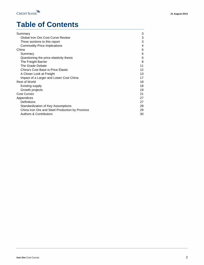
DISCLOSURE APPENDIX CONTAINS IMPORTANT DISCLOSURES, ANALYST CERTIFICATIONS, INFORMATION ON TRADE ALERTS, ANALYST MODEL PORTFOLIOS AND THE STATUS OF NON-U.S ANALYSTS. FOR OTHER

IMPORTANT DISCLOSURES, visit www.creditsuisse.com/researchdisclosures or call +1 (877) 291-2683 for Credit Suisse Equity Research disclosures and visit https://firesearchdisclosure.credit-suisse.com or call +1 (212) 538- 7625 for Credit Suisse Fixed Income Research disclosures. US Disclosure: Credit Suisse does and seeks to do business with companies covered in its research reports. As a result, investors should be aware that the Firm may have a conflict of interest that could affect the objectivity of this report. Investors should consider this report as only a single factor in making their investment decision.

CREDIT SUISSE SECURITIES RESEARCH & ANALYTICS BEYOND INFORMATION®

Client-Driven Solutions, Insights, and Access

21 August 2013

Americas/United States

Securities Research & Analytics

Iron Ore Cost Curves Connections Series

Global Update and a Closer Look at China

We expect the iron ore price to move lower in coming years as new projects

from Australia and Brazil hit the seaborne market. As this happens, investor

attention is likely to focus on the cost curve, and the role it plays in supporting

the iron ore price. This report explores the subject in some detail.

Exhibit 1: Global Cost Curve, 2013 Estimate Red=Consensus 2013 price, Blue=Credit Suisse 2013 price, Grey=Credit Suisse 2012 cost curve

BHP.AX CLF FMG.AX KIOJ.J RIO.AX VALE.N China Other Reported Cash Cost (FOB)

All-In Cash Cost (FOB)

All-In 62% IODEX equiv (CFR)

0

20

40

60

80

100

120

140

160

0 100 200 300 400 500 600 700 800 900 1000 1100 1200 1300

US

$ p

er

dry

metr

ic t

onne

Million tonnes per annum

Source: Company data, Credit Suisse Securities Research & Analytics and Commodities

Research estimates.

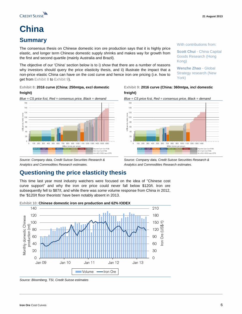
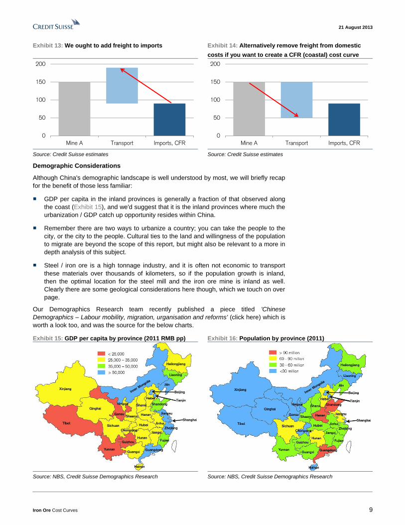
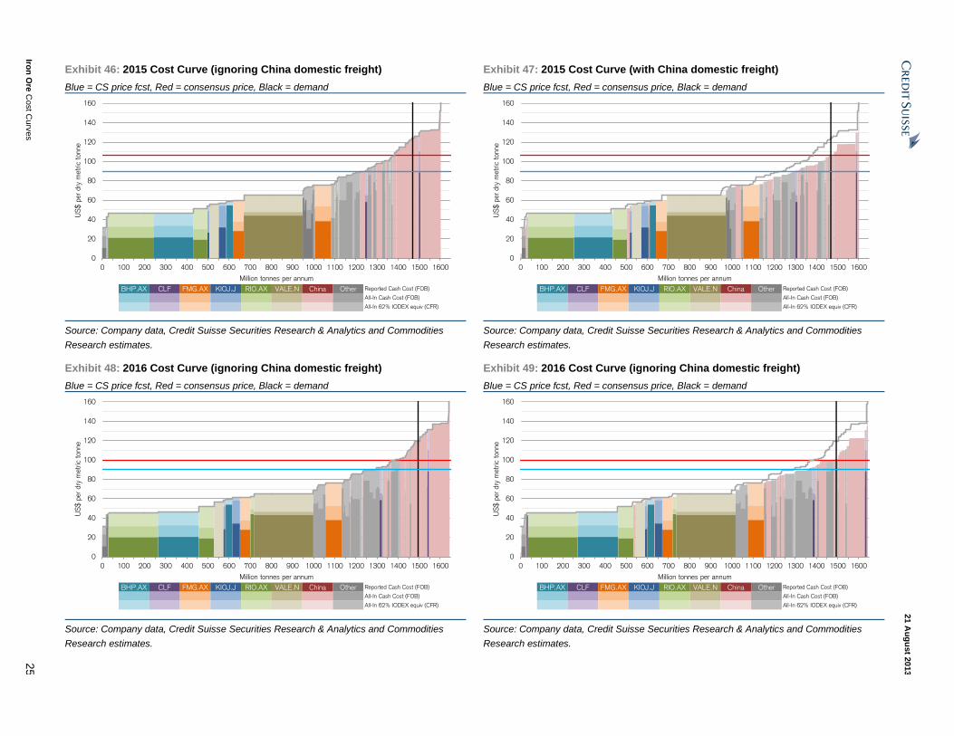
Perhaps the most differentiated section of this report is our analysis of the Chinese domestic cost curve. We provide reason for investors to query consensus thinking on Chinese volumes, and demonstrate the importance of

considering domestic freight from a cost curve perspective.

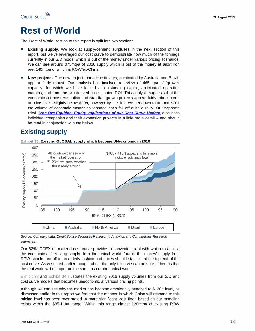
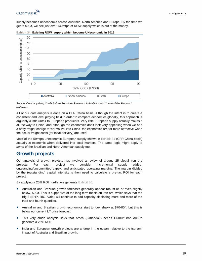
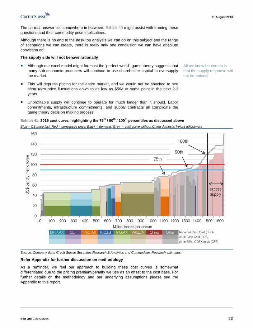
Our Rest of World analysis identifies ~140mtpa of existing supply which would

be uneconomic by 2016 at $90/t; however, we believe that the economics of 'Big 3' expansion tonnage from Australia and Brazil is robust at, or even slightly below, the same $90/t level. Please refer to our separate equities report for a

discussion of specific stocks.

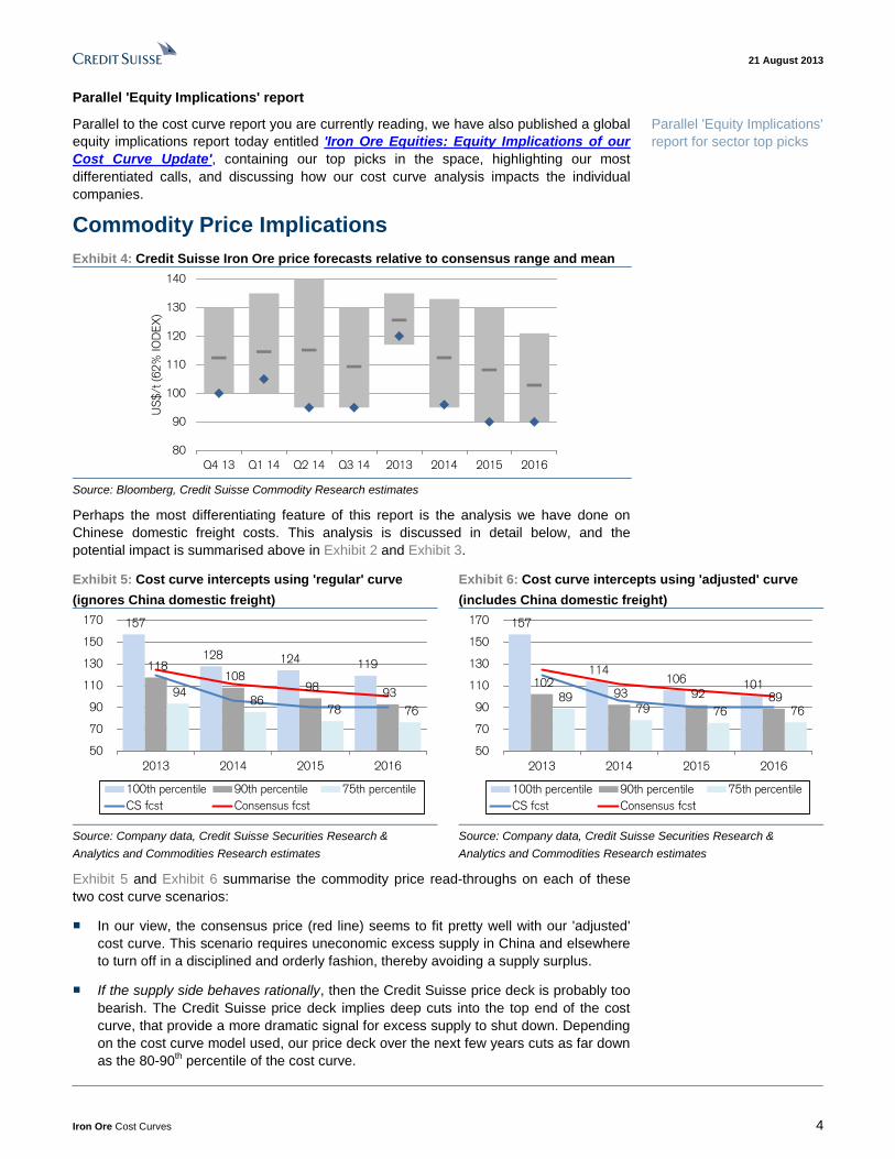
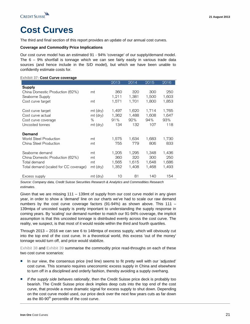
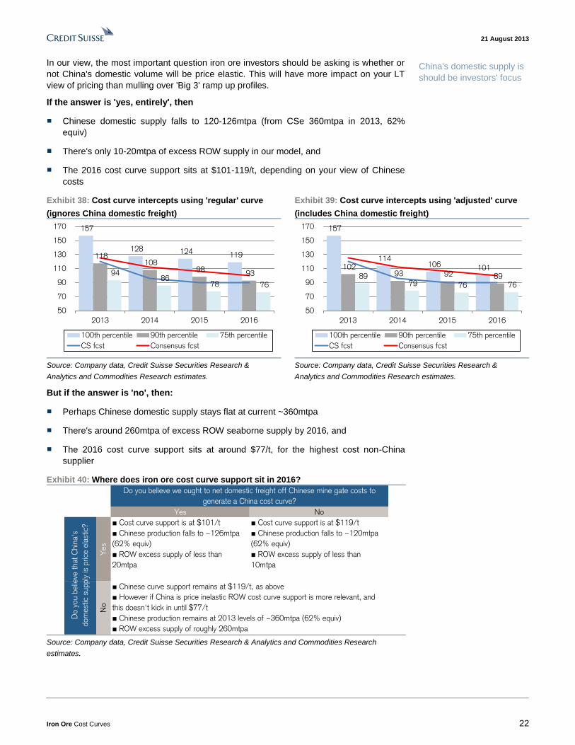
If the supply side behaves rationally, then consensus price forecasts correlate pretty well with our cost curve model over 2014-2016, but our own price forecasts cut well into the 80-90

th percentile of the cost curve. We demonstrate

how one’s view on China can generate 2016 price expectations anywhere from $76 to 119/t based on cost curve support.

The Credit Suisse Connections Series

leverages our exceptional breadth of

macro and micro research to deliver

incisive cross-sector and cross-border

thematic insights for our clients.

Equity Analysts

Nathan Littlewood

416 352 4585

Paul McTaggart

61 2 8205 4698

Matthew Hope

61 2 8205 4669

Ivano Westin

55 11 3701 6318

Liam Fitzpatrick

44 20 7883 8350

James Gurry

44 20 7883 7083

Neelkanth Mishra

91 22 6777 3716

Semyon Mironov

7 495 662 8510

Trina Chen

852 2101 7031

Fixed Income Analysts

Marcus Garvey

44 20 7883 4787

Andrew Shaw

65 6212 4244

http://release.theplatform.com/content.select?pid=jJTCPbU_trrv1REM5sqz0qqWxw2ziDsJ&UserName=Unknown

21 August 2013

Iron Ore Cost Curves 2

Table of Contents Summary 3

Global Iron Ore Cost Curve Review 3 Three sections to this report 3 Commodity Price Implications 4

China 6 Summary 6 Questioning the price elasticity thesis 6 The Freight Barrier 8 The Grade Debate 11 China's Cost Base is Price Elastic 12 A Closer Look at Freight 13 Impact of a Larger and Lower Cost China 17

Rest of World 18 Existing supply 18 Growth projects 19

Cost Curves 21 Appendices 27

Definitions 27 Standardization of Key Assumptions 28 China Iron Ore and Steel Production by Province 29 Authors & Contributors 30

21 August 2013


Summary Global Iron Ore Cost Curve Review

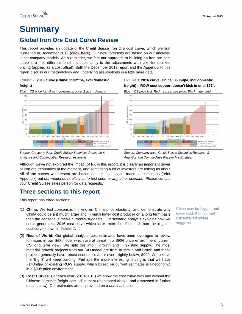
This report provides an update of the Credit Suisse Iron Ore cost curve, which we first

published in December 2012 (click here). Our new forecasts are based on our analysts'

latest company models. As a reminder, we feel our approach to building an iron ore cost

curve is a little different to others due mainly to the adjustments we make for realized

pricing (applied as a cost offset). Both the December 2012 report and the Appendix to this

report discuss our methodology and underlying assumptions in a little more detail.

Exhibit 2: 2016 curve (China: 250mtpa, excl domestic

freight)

Blue = CS price fcst, Red = consensus price, Black = demand

Exhibit 3: 2016 curve (China: 360mtpa, incl domestic

freight) – ROW cost support doesn't kick in until $77/t





0

20

40

60

80

100

120

140

160

0 100 200 300 400 500 600 700 800 900 1000 1100 1200 1300 1400 1500 1600

US

$ p

er

dry

metr

ic t

onne





0

20

40

60

80

100

120

140

160

0 100 200 300 400 500 600 700 800 900 1000 1100 1200 1300 1400

US

$ p

er

dry

metr

ic t

onne


Source: Company data, Credit Suisse Securities Research &

Analytics and Commodities Research estimates.



Although we've not explored the impact of FX in this report, it is clearly an important driver

of iron ore economics at the moment, and something a lot of investors are asking us about.

All of the curves we present are based on our 'base case' macro assumptions (refer

Appendix) but our model does allow us to test spot, or any other scenario. Please contact

your Credit Suisse sales person for data requests.

Three sections to this report

This report has three sections:

(1) China: We test consensus thinking on China price elasticity, and demonstrate why

China could be a i) much larger and ii) much lower cost producer on a long term basis

than the consensus thesis currently suggests. Our scenario analysis explains how we

could generate a 2016 cost curve which looks more like Exhibit 3 than the 'regular'

cost curve shown in Exhibit 2.

(2) Rest of World: Our global analysts' cost estimates have been leveraged to review

tonnages in our S/D model which are at threat in a $90/t price environment (current

CS long term view). We split this into i) growth and ii) existing supply. The most

material 'growth' projects from our S/D model are from Australia and Brazil, and these

projects generally have robust economics at, or even slightly below, $90/t. We believe

the 'Big 3' will keep building. Perhaps the more interesting finding is that we have

~140mtpa of existing ROW supply, which based on current estimates is uneconomic

in a $90/t price environment.

(3) Cost Curves: For each year (2013-2016) we show the cost curve with and without the

Chinese domestic freight cost adjustment (mentioned above, and discussed in further

detail below). Our estimates are all provided on a nominal basis.

China may be bigger, and

lower cost, than current

consensus thinking

suggests

https://doc.research-and-analytics.csfb.com/docView?sourceid=em&document_id=x487653&serialid=e%2bvKc7taBS3VZwcbqnGCxUlTUGTWT6If2gXtLPIuKZw%3d

21 August 2013


Parallel 'Equity Implications' report

Parallel to the cost curve report you are currently reading, we have also published a global

equity implications report today entitled 'Iron Ore Equities: Equity Implications of our

Cost Curve Update', containing our top picks in the space, highlighting our most

differentiated calls, and discussing how our cost curve analysis impacts the individual

companies.

Commodity Price Implications

Exhibit 4: Credit Suisse Iron Ore price forecasts relative to consensus range and mean

80

90

100

110

120

130

140

Q4 13 Q1 14 Q2 14 Q3 14 2013 2014 2015 2016

US

$/t

(6

2%

IO

DE

X)

Source: Bloomberg, Credit Suisse Commodity Research estimates

Perhaps the most differentiating feature of this report is the analysis we have done on

Chinese domestic freight costs. This analysis is discussed in detail below, and the

potential impact is summarised above in Exhibit 2 and Exhibit 3.

Exhibit 5: Cost curve intercepts using 'regular' curve

(ignores China domestic freight)

Exhibit 6: Cost curve intercepts using 'adjusted' curve

(includes China domestic freight)

157

128 124 119 118 108

98 93 94

86 78 76

50

70

90

110

130

150

170

2013 2014 2015 2016

100th percentile 90th percentile 75th percentile

CS fcst Consensus fcst

157

114 106 101 102

93 92 89 89 79 76 76

50

70

90

110

130

150

170

2013 2014 2015 2016




Analytics and Commodities Research estimates


Analytics and Commodities Research estimates

Exhibit 5 and Exhibit 6 summarise the commodity price read-throughs on each of these

two cost curve scenarios:

■ In our view, the consensus price (red line) seems to fit pretty well with our 'adjusted'

cost curve. This scenario requires uneconomic excess supply in China and elsewhere

to turn off in a disciplined and orderly fashion, thereby avoiding a supply surplus.

■ If the supply side behaves rationally, then the Credit Suisse price deck is probably too

bearish. The Credit Suisse price deck implies deep cuts into the top end of the cost

curve, that provide a more dramatic signal for excess supply to shut down. Depending

on the cost curve model used, our price deck over the next few years cuts as far down

as the 80-90th percentile of the cost curve.

Parallel 'Equity Implications'

report for sector top picks


21 August 2013


In our view, the most important question iron ore investors should be asking is whether or

not China's domestic volume will be price elastic. This will have more impact on your LT

view of pricing than mulling over 'Big 3' ramp up profiles.

If the answer is 'yes, entirely', then

■ Chinese domestic supply falls to 120-126mtpa (from CSe 360mtpa in 2013, 62%

equiv)

■ There's only 10-20mtpa of excess ROW supply in our model, and

■ The 2016 cost curve support sits at $101-119/t, depending on your view of Chinese

costs

But if the answer is 'no', then:

■ Perhaps Chinese domestic supply stays flat at current ~360mtpa

■ There's around 260mtpa of excess ROW seaborne supply by 2016, and

■ The 2016 cost curve support sits at around $77/t, for the highest cost non-China

supplier

The correct answer lies somewhere in between. Exhibit 7 might assist with framing these

questions and their commodity price implications.

Exhibit 7: Where does iron ore cost curve support sit in 2016?

Yes No

Yes

■ Cost curve support is at $101/t

■ Chinese production falls to ~126mtpa

(62% equiv)

■ ROW excess supply of less than

20mtpa



(62% equiv)


10mtpa

No

Do you believe we ought to net domestic freight off Chinese mine gate costs to

generate a China cost curve?

■ Chinese curve support remains at $119/t, as above

■ However if China is price inelastic ROW cost curve support is more relevant, and

this doesn't kick in until $77/t

■ Chinese production remains at 2013 levels of ~360mtpa (62% equiv)

■ ROW excess supply of roughly 260mtpa

Do y

ou b

elie

ve t

hat C

hin

a's

dom

est

ic s

upply

is p

rice

ela

stic

?

Source: Company data, Credit Suisse Securities Research & Analytics and Commodities Research

estimates.

Although there is no end to the desk top analysis we can do on this subject and the range

of scenarions we can create, there is really only one conclusion we can have absolute

conviction on…

The supply side will not behave rationally

■ Although our excel model might forecast the 'perfect world', game theory suggests that

many sub-economic producers will continue to use shareholder capital to oversupply

the market.

■ This will depress pricing for the entire market, and we would not be shocked to see

short term price fluctuations down to as low as $50/t at some point in the next 2-3

years.

■ Unprofitable supply will continue to operate for much longer than it should. Labor

commitments, infrastructure commitments, and supply contracts all complicate the

game theory decision making process.

China's domestic supply is

should be investors' focus

All we know for certain is

that the supply response will

not be rational

21 August 2013


China Summary

The consensus thesis on Chinese domestic iron ore production says that it is highly price

elastic, and longer term Chinese domestic supply shrinks and makes way for growth from

the first and second quartile (mainly Australia and Brazil).

The objective of our 'China' section below is to i) show that there are a number of reasons

why investors should query the price elasticity thesis, and ii) illustrate the impact that a

non-price elastic China can have on the cost curve and hence iron ore pricing (i.e. how to

get from Exhibit 8 to Exhibit 9).

Exhibit 8: 2016 curve (China: 250mtpa, excl domestic

freight)


Exhibit 9: 2016 curve (China: 360mtpa, incl domestic

freight)





0

20

40

60

80

100

120

140

160

0 100 200 300 400 500 600 700 800 900 1000 1100 1200 1300 1400 1500 1600

US

$ p

er

dry

metr

ic t

onne





0

20

40

60

80

100

120

140

160

0 100 200 300 400 500 600 700 800 900 1000 1100 1200 1300 1400

US

$ p

er

dry

metr

ic t

onne






Questioning the price elasticity thesis

This time last year most industry watchers were focused on the idea of "Chinese cost

curve support" and why the iron ore price could never fall below $120/t. Iron ore

subsequently fell to $87/t, and while there was some volume response from China in 2012,

the '$120/t floor theorists' have been notably absent in 2013.

Exhibit 10: Chinese domestic iron ore production and 62% IODEX

0

30

60

90

120

150

180

210

0

20

40

60

80

100

120

140

Jan 09 Jan 10 Jan 11 Jan 12 Jan 13

Iron O

re (

US

$/t

)

Month

ly d

om

est

ic C

hin

ese

pro

duct

ion (

mt)

Volume Iron Ore

Source: Bloomberg, TSI, Credit Suisse estimates

With contributions from:

Scott Chui - China Capital

Goods Research (Hong

Kong)

Wenzhe Zhao - Global

Strategy research (New

York)

21 August 2013


At the extremes, we have seen estimates for long term Chinese domestic supply ranging

from 200mtpa up to 550mtpa – i.e. a 350mtpa spread. One's view on China's domestic

industry is comparable in magnitude to 100% of Vale, the world's largest iron ore producer.

We'd suggest that an analysis of China's domestic iron ore industry is more relevant to

forming a view on the long term commodity price than debating bullish/bearish scenarios

for Big 3 ramp up.

Reasons why investors should question China's price elasticity

We can see a number of reasons to question the traditional Chinese price elasticity thesis:

■ The freight barrier. Although most iron ore investors are accustomed to thinking

about mine to port rail costs and seaborne freight, we are surprised that Chinese

domestic freight doesn't get as much attention. The cost of freight in China does

however 'shelter' a large portion of the domestic industry (~160mtpa of 62% equivalent

supply comes from inland provinces), effectively creating a barrier to entry for import

competition.

■ The Grade Debate. Statistical evidence to support a price / production relationship is

weak, and we hypothesize whether China's observable grade depletion trend could in

fact be a reversable trend. If so, mining at higher grades will structurally change the

shape of the cost curve as we know it today.

■ China's cost base is price elastic. Although we think the price elasticity of Chinese

volumes is low, a look at regional cost structures shows that the price elasticity of

China's cost base is probably one of the highest in the world. 40% of the China cost

base is a function of the iron ore price. As prices move lower, these price-linked costs

will decrease.

Each of these topics is discussed in more detail below.

A more comprehensive analysis of this subject would also look at the growing importance

of captive SOE supply. Although the ownership structure of the iron ore industry is a little

different to that of steel, steel investors will be well aware that when it comes to China a

lack of profitability is not sufficient to see excess capacity removed. China does not always

behave as a market based economy.

Reasons to question the

consensus thinking on

China

21 August 2013


The Freight Barrier

Iron Ore growth has been inland, not along the coast

It is well known that over the past 5 years China's steel industry has been moving towards

the coast (Exhibit 11). Less well known, but an equally relevant trend in our view, is that

growth across China's Inland iron ore provinces has outpaced that of coastal provinces.

The consequence of this inland iron ore growth is that Coastal provinces now only

contribute ~55% of domestic supply, down from over 70% just a few years ago.

Exhibit 11: Percent production from Coastal provinces Exhibit 12: YoY growth in coastal / inland iron ore

volumes

45%

50%

55%

60%

65%

70%

75%

2004 2005 2006 2007 2008 2009 2010 2011 2012 2013

Contr

ibutio

n fro

m C

oas

tal

Pro

vince

s

Iron Ore Steel

-20%

0%

20%

40%

60%

80%

100%

2005 2006 2007 2008 2009 2010 2011 2012 2013

Coastal Inland

Source: Bloomberg, Credit Suisse estimates Source: Bloomberg, Credit Suisse estimates

Iron Ore investors should appreciate the importance of freight when understanding mine

economics. While many of us are quite used to making freight adjustments between the

mine and port, or the port (FOB) and the customer (CFR), most investors neglect to

consider freight and logistics costs at the customer end of the supply chain.

Ignoring freight costs within China is akin to assuming that the entire country fits on the

head of a pin. In our view, an understanding of China's domestic freight industry is critical

to understanding the longer term competitive dynamic between imported and domestic

material. Consider the following illustrative example:

Imagine 'Mine A' which has mine gate costs of $150/t and typically services a local steel

mill. Due to being located thousands of kilometres inland, transport costs between Mine A

and the nearest port are say $100/t.

■ Traditional thinking would suggest that in a $90/t CFR world our $150/t mine is $60/t

out of the money, and we'd take it out of our S/D model, but

■ For imports to actually compete with, and displace, Mine A their delivered cost is 90 +

100 = $190/t (Exhibit 13). In other words Mine A is actually $40/t in the money (190 –

150).

Alternatively, if we wanted to accurately depict the economics of competing supply on a

CFR (coastal) basis, we could remove the same $100/t freight cost to get a CFR

equivalent cost for Mine A of $50/t (Exhibit 14). Again, this puts Mine A $40/t in the money

relative to our $90/t imports.

The $100/t freight example above is just an example and actual costs are actually

considerably lower. At the end of this section we develop a province by province freight

cost model and show what the cost curve looks like with / without this adjustment (i.e. we

replace the $100/t with proper estimates for each province).

21 August 2013


Exhibit 13: We ought to add freight to imports Exhibit 14: Alternatively remove freight from domestic

costs if you want to create a CFR (coastal) cost curve

0

50

100

150

200

Mine A Transport Imports, CFR

0

50

100

150

200

Mine A Transport Imports, CFR

Source: Credit Suisse estimates Source: Credit Suisse estimates

Demographic Considerations

Although China's demographic landscape is well understood by most, we will briefly recap

for the benefit of those less familiar:

■ GDP per capita in the inland provinces is generally a fraction of that observed along

the coast (Exhibit 15), and we'd suggest that it is the inland provinces where much the

urbanization / GDP catch up opportunity resides within China.

■ Remember there are two ways to urbanize a country; you can take the people to the

city, or the city to the people. Cultural ties to the land and willingness of the population

to migrate are beyond the scope of this report, but might also be relevant to a more in

depth analysis of this subject.

■ Steel / iron ore is a high tonnage industry, and it is often not economic to transport

these materials over thousands of kilometers, so if the population growth is inland,

then the optimal location for the steel mill and the iron ore mine is inland as well.

Clearly there are some geological considerations here though, which we touch on over

page.

Our Demographics Research team recently published a piece titled 'Chinese

Demographics – Labour mobility, migration, urganisation and reforms' (click here) which is

worth a look too, and was the source for the below charts.

Exhibit 15: GDP per capita by province (2011 RMB pp) Exhibit 16: Population by province (2011)

Source: NBS, Credit Suisse Demographics Research Source: NBS, Credit Suisse Demographics Research

https://plus.credit-suisse.com/r/qircfU

21 August 2013


Geological considerations

■ Globally, iron ore is dominantly related to banded iron formation (BIF), which is

essentially repeated thin layers of iron and silica one on top of the other. BIF is

exclusively found in ancient Precambrian rocks (and mainly formed in the time period

of 2500 to 1800 million years ago – the Archean and early Proterozoic eons). BIF will

not be found in younger rocks. Hebei, Shandong and Jilin Provinces have BIF along

the Northern China Platform, and this is the major centre of iron ore production and

exploration in China. Coincidentally, this iron ore province is also proximal to the

coast. The pink 'Archeozoic' areas in Exhibit 17 illustrate the exposures of ancient

rocks that can host BIF.

Exhibit 17: Geological Map of China

Source: China Geological Survey

■ Other less voluminous, but useful iron ore in China is found in skarn deposits, which

are small but high grade. These are widespread, and being high grade will be widely

exploited.

■ Thirdly there are the magmatic deposits exemplified by the mighty iron–titanium-

vanadium Panzihua deposit in Sichuan. Panzihua is billions of tonnes in size and

mined by a number of companies for all three minerals.

Given the importance of Panzihua and the BIFs for China’s iron ore production, we likely

already know the locations of Chinese iron ore mines which will be in operation 5 or even

10 years from now - as they will be defined by geology, and not demographics.

We'd be surprised if iron ore production from China's Inland provinces will be decreasing

as we look forward. Our broad assumption is that inland mines are servicing inland steel

mills, and for various reasons it can be difficult for imports to penetrate these markets in

volume. We estimate that over 160mtpa of China's 360mtpa (62% equivalent) domestic

supply (45%) is coming from these inland provinces at the moment, so any conversation

about China's price elasticity longer term should arguably be constrained to coastal

volumes. Of the ~200mtpa being produced along the coast, a large portion will be SOE

owned and a large portion will have better costs than imports. For the same reasons that

21 August 2013


the steel industry hasn't responded to a lack of profitability, coastal iron ore mines may not

respond to a low price environment either.

The Grade Debate

Historical analysis suggests that China's domestic ore tonnes mined are somewhat price

elastic (Exhibit 18). Perhaps unsurprisingly given our comments above, there is a higher

degree of price elasticity (slope of the trend line) for coastal provinces than there is inland

provinces.

Exhibit 18: Ore Volume against Iron Ore Price Exhibit 19: Contained Iron against Iron Ore Price

y = 0.1216x + 22.227

y = 0.1539x + 37.482

10

20

30

40

50

60

70

50 75 100 125 150 175 200

Ore

Volu

me (

mt)

Iron Ore Price 62% IODEX

Inland Coastal

y = 0.012x + 4.6374

y = 0.01x + 8.4792

2.5

5.0

7.5

10.0

12.5

15.0

50 75 100 125 150 175 200

Conta

ined Iro

n V

olu

me (

mt)

Iron Ore Price 62% IODEX

Inland Coastal

Source: Bloomberg, TSI, Credit Suisse estimates Source: Bloomberg, TSI, Credit Suisse estimates

There is another adjustment that can be made to this data however. Rather than just

looking at crude (as reported) ROM tonnes (Exhibit 18), we can adjust for contained iron

(i.e. grade) as well, as per Exhibit 19. Although the low correlation coefficients don't really

change much, the interesting thing about Exhibit 19 is that the price elasticity is far lower.

In fact it is pretty close to zero (again, we are referring to the slope/gradient of the trend

line here).

Exhibit 20: Chinese domestic iron ore grades against

commodity price

Exhibit 21: Global gold grades and commodity price

40

80

120

160

200

2400%

10%

20%

30%

40%

50%

60%

70%

Jan

03

Jan

04

Jan

05

Jan

06

Jan

07

Jan

08

Jan

09

Jan

10

Jan

11

Jan

12

Jan

13

62

% IO

DE

X -

INV

ER

TE

D

Implie

d d

om

est

ic o

re g

rade

Grade % Fe 62% IODEX US$/t

0

300

600

900

1,200

1,500

1,8001.0

1.2

1.4

1.6

1.8

2.0

2.2

1992 1997 2002 2007 2012

Gold

Price

-IN

VE

RTE

D

Ave

rage G

lobal

Gold

Gra

de (

g/t

)

Grade g/t Gold Price $/oz

Source: Bloomberg, TSI, Credit Suisse estimates Source: Wood Mackenzie, Credit Suisse estimates

The data seems to suggest that as the price of iron ore fluctuates, the ore tonnes change,

but the contained iron does not. We suspect this observation may be the aggregate effect

of a number of drivers:

■ Low grade / high cost mines enter the market on an opportunistic basis when prices

are high, dragging down the average head grade across the country.

21 August 2013


■ To the extend possible, mine plans are modified to exploit lower grade/high cost

tonnes when prices are high and the mine can remain cash flow positive.

■ On a longer term basis, we could also be observing a deliberate reallocation of mining

resources from high to low grade mines in response to price.

Similar price / grade relationships can be observed in most other commodities. Exhibit 21

illustrates the point with gold.

Just like any other iron ore region we've no doubt that depletion plays a part, but

remember China is one of the largest iron ore producers in the world. The country holds

billions and billions of tonnes in iron ore resources. Given that the average head grade

from the Pilbara has fallen by perhaps 1 percent over the past decade, it seems

improbable that China's multi-billion tonne resource base has fallen by 15-20% over the

same period. The grade/tonnage curve simply can't be that steep.

If part of China's observed grade trend can be reversed, then costs are likely to fall. A

mine that extracts ore at say 15% ROM (run of mine, i.e. unprocessed ore) and produces

a 64% Fe concentrate for cash costs of say $120/t, could produce the same 64%

concentrate at $70-80/t if it was mining 25-30% ROM ore.

We do not capture the impact of a changing grade profile in our cost curve. Our numbers

essentially assume grade is kept flat.

China's Cost Base is Price Elastic

Not only could a change of mined grade have a favorable impact on Chinese production

costs, but we think that in an absolute sense a lower price environment will do the same.

Exhibit 22: Cost Structure break down, by country

0%

20%

40%

60%

80%

100%

Australia Brazil Canada China Guinea India Liberia Russia Sierra

Leone

South

Africa

Ukraine USA

Mining Costs ($/tonne) Processing Costs ($/tonne) Transport Costs ($/tonne)

Pelletising Costs ($/tonne) Port Costs ($/tonne) Overheads ($/tonne)

Royalty and Levies ($/tonne)

Source: Wood MacKenzie, Credit Suisse estimates

According to Wood Mac estimates, roughly 40% of China's average production costs are

associated with 'overheads, royalties and levies'. We consider most of this likely to be a

derivative of the commodity price. 40% price-linked costs is higher than any other country

in the world except maybe India, with the global average being closer to 20% (Exhibit 22).

We suspect that a lot of this 40% represents 'price participation' on behalf of the

authorities, much of which is likely opportunistic in nature and likely to reduce as prices fall

and margins reduce. Anecdotes from China iron ore mine visits include people standing on

the side of the road charging a toll to truck drives because they know they can afford it.

When the price falls the truck driver can't afford the toll, and the person on the side of the

road goes away and does something else.

Simply put, the cost structure of the Chinese iron ore industry is probably one of the most

price-elastic iron ore cost structures in the world. If you believe iron ore prices are

lowering, you should expect all-in Chinese costs to more lower as well. For the purposes

21 August 2013


of our cost curve model we do not capture any of this cost elasticity. For conservatism, we

in fact model 5%pa inflation on Chinese costs.

A Closer Look at Freight

The previous few pages have hopefully given readers cause to see why longer term China

might not only be a bigger producer, but also a lower cost producer than consensus

thinking suggests. Not only do we expect Chinese production costs to fall much more

quickly than ROW putting more supply back in the money, but further we feel that the

relevance of price in determining Chinese production decisions (elasticity) is overstated.

China is not a market-based economy.

The following section illustrates the potential cost curve impact of our domestic freight

discussion above. Carrying on from the $150/t Mine A example with the $100/t freight

costs, the following section actually derives provincial level estimates for both.

Estimating the impact of domestic freight costs

Exhibit 23: Chinese freight transport, by mode Exhibit 24: Chinese 'Metal Ores' transported by rail

0%

20%

40%

60%

80%

100%

1970 1980 1990 2000 2008 2012

Railway Highway Waterway Air Pipeline

0

50

100

150

200

250

300

350

400

1992 1995 1998 2001 2004 2007 2010

Source: Company data, Credit Suisse Equity Research (18 June

2013)

Source: CEIC, Credit Suisse Equity Research (18 June 2013)

Although Waterway and Highway freight has taken significant market share from rail over

the past few decades (Exhibit 23), we suspect that rail remains the main method for

transporting iron ore over long distances given that:

■ Rail is significantly faster than water

■ Highway / trucking is the main method used over short distances, but over longer

distances its costs are likely prohibitive.

Trucking is used extensively in Shanxi and the western part of Hebei, and our China team

estimate this could cost as much as $10-20/t.

21 August 2013


Rail costing model

With the help of our China Industrials team we've built a simple Chinese rail cost model, as

summarized below.

Exhibit 25: Chinese Rail Freight costing model

Haulage

Distance

km Rmb/t Rmb/t/km Rmb/t Rmb/t/km Rmb/t Rmb/t/km Rmb/t Rmb/t/km Rmb/t Rmb/t/km Rmb/t Rmb/t/km US$/t US$/t/km

50 13.8 0.28 3.77 0.08 1.65 0.033 0.60 0.012 22.4 0.45 42.22 0.84 6.90 0.138

100 13.8 0.14 7.53 0.08 3.30 0.033 1.20 0.012 22.4 0.22 48.23 0.48 7.88 0.079

500 13.8 0.03 37.65 0.08 16.50 0.033 6.00 0.012 22.4 0.04 96.35 0.19 15.74 0.031

1000 13.8 0.01 75.30 0.08 33.00 0.033 12.00 0.012 22.4 0.02 156.50 0.16 25.57 0.026

Total TotalBase rate 1

(variable)Base rate 2 (fixed)

Construction fund

surcharge

Electrification

surchargeLoading/unloading

Source: China Ministry of Railway, Credit Suisse estimates

Over short distances, the loading/unloading costs associated with rail are likely to make

trucking more attractive, however on a pure operating cost basis rail looks more attractive

for haulage in excess of 100km.

Exhibit 26: China Railway Map, from 12th

Five Year Plan

Source: Chinese Ministry of Railways

The Three Gorges dam and lock system allows penetration of imported ores all the way up

to Chongqing in 10kt vessels. BHP.AX does in fact sell its seaborne marketing into

Sichuan province via this route.

We don't have a waterway cost model, but it is our understanding that barging costs are in

the order of $0.02 per tonne km. Nominating the mode of transport might therefore be

relevant for capacity/volume based analysis, but for our high level economic based

analysis the comparable costs mean that we do not need to differentiate between the two.

The final step in our domestic freight cost analysis is to estimate distances.

■ Rather than getting lost in the detail, we've done this on a provincial basis by

considering the most likely port option for each province. Clearly in some cases there

are multiple options, and for some of the larger provinces there would be significant

21 August 2013


variance from one side of the province to the other, but the averages we've used are

summarized in Exhibit 27.

■ Exhibit 26 is the Ministry of Rail map from China's 12th year plan, and so far as

possible we've tried to keep 'googlemaps' routing consistent with rail routing.

Exhibit 27 combines our estimated distances with our freight costing model (Exhibit 25) to

generate a $/t rail cost / net back estimate for each province. Were imported material to be

competing with domestic material in each of these provinces, the below seems to be a

reasonable assumption regarding potential routing. This final freight column below has

been removed /netted off our mine gate cost estimates in the scenarios which follow.

Exhibit 27: Chinese domestic freight costs – Credit Suisse estimates

Province ROM 2012 Output (Mt) Port Distance (km) Freight (US$/t)

Anhui 46 Shanghai 470 15

Beijing 20 Tianjin 140 9

Fujian 14 Quanzhou 200 10

Gansu 11 Qigdao 1,830 43

Guangdong 22 Guangzhou 50 7

Guangxi 4 Zhanjiang 330 13

Guizhou 1 Zhanjiang 880 24

Hainan 6 Basuo 50 7

Hebei Low/Mid 184 Tianjin 334 13

Hebei High 347 Tianjin 334 13

Heilongjiang 5 Dalian 935 25

Henan 15 Rizhao 575 17

Hubei 23 Liangyungang 840 23

Hunan 8 Xiamen 870 23

Inner Mongolia 92 Tianjin 620 18

Jiangsu 2 Shanghai 150 9

Jiangxi 19 Xiamen 690 20

Jilin 17 Dalian 690 20

Liaoning Low/Mid 25 Dalian 360 13

Liaoning High 129 Dalian 360 13

Qinghai 2 Tianjin 1,720 40

Shaanxi 12 Rizhao 1,000 26

Shandong 154 Qingdao 100 8

Shanxi 81 Tianjin 550 17

Sichuan 163 Rizhao 1,750 41

Xinjiang 29 Tianjin 3,200 70

Yunnan 26 Zhanjiang 1,100 28

Zhejiang 2 Shanghai 170 9

Mean (volume weighted) 571 17 Source: Company data, Credit Suisse Securities Research & Analytics and Commodities Research

estimates.

The same data is shown in Exhibit 28, and in the Appendix to this report we have a map of

China which shows both iron ore and steel production by province.

Regarding Exhibit 28:

■ The diagonal lines illustrate the divide between material which is economic and

material which is not (based on the freight net back from coast) at $80, $100 and

$120/t. y axis value less x axis value = grey line.

■ On a 2013 basis, our methodology implies that 36% / 129mtpa of Chinese domestic

tonnage is uneconomic at $100/t, 49% / 177mtpa at $90/t, and 70% / 251mtpa at $80/t

■ A more comprehensive analysis of this subject would look at ownership structures (i.e.

SOE v private) and raw material switching costs for the steel mill. As any steel analyst

will tell you, just because an industry is unprofitable in China doesn't mean it will cease

to produce.

21 August 2013


■ Also recall our earlier discussion of cost elasticity. To demonstrate the sensitivity to

costs, consider a scenario where the entire Chinese industry were capable of lowering

their cost base by 20%. The volumes quoted above become 0.5% / 2mtpa at $100/t,

2% / 9mtpa at $90/t, and 37% / 132mtpa at $80/t.

Exhibit 28: Chinese provincial iron ore production

Bubble diameter represents production (mtpa), and 80/100/120 lines indicate the theoretical

divide between tonnage which would be economic, and tonnage which is not

20

40

60

80

100

120

140

160

180

0 10 20 30 40 50 60 70 80

Min

e G

ate

Cost

(U

S$/t

)

Estimated freight net back, from closest port (US$/t)

$120

$80

$100


estimates.

Mine verse Steel Mill net back?

■ We have 'netted back' the China domestic freight costs based on the mine location,

and not the steel mill location. Readers would be right to query whether this is the best

approach, given that it is the steel mills' location which determines the clearing price

for iron ore and it is at the steel mill that the imports v domestic raw material battle

takes place.

■ Our broad assumption is that inland mines are servicing inland steel mills. Exhibit 11

shows that there is only a 7% difference between the volume of iron ore produced by

coastal provinces (53%) and the volume of steel produced by coastal provinces (60%).

Therefore using a steel mill rather than iron ore mine net back would only change our

overall freight overlay by 7%, which we consider less than our forecasting error.

In the next section of this report we use our in house model to demonstrate how the above

concepts may impact the cost curve.

21 August 2013


Impact of a Larger and Lower Cost China

Using our 2016 cost curve as a case study, we set out four basic steps:

■ Step 1 / Exhibit 29: start with a 'regular' iron ore cost curve (in which domestic freight

costs are ignored). We've used the Credit Suisse 2016 estimates as a case study. The

Step 1 data is repeated on Step 2 – 4 charts as a grey outline.

■ Step 2 / Exhibit 30: Adjust Chinese domestic production for domestic freight costs –

i.e. net them back to a CFR equivalent cost

Exhibit 29: Step 1: Start with a 'regular' 2016 cost curve


Exhibit 30: Step 2: Adjust China Cost base for domestic

freight




0

20

40

60

80

100

120

140

160

0 100 200 300 400 500 600 700 800 900 1000 1100 1200 1300 1400 1500 1600

US

$ p

er

dry

metr

ic t

onne


Cost curve support at $120/t




0

20

40

60

80

100

120

140

160

0 100 200 300 400 500 600 700 800 900 1000 1100 1200 1300 1400 1500 1600

US

$ p

er

dry

metr

ic t

onne







■ Step 3 / Exhibit 31: Instead of shrinking Chinese supply to 250mtpa (as per our

existing S/D model), keep it flat at 360mtpa (CSe 2013, 62% equivalent).

■ Step 4 / Exhibit 32: make room for the extra 110mtpa of Chinese domestic material by

removing 200mtpa ROW supply

Exhibit 31: Step 3: Keep Chinese production flat at

360mtpa (rather than reducing to 250mtpa)

Exhibit 32: Step 4: Remove excess ROW supply to

balance supply with demand




0

20

40

60

80

100

120

140

160

0 100 200 300 400 500 600 700 800 900 1000 1100 1200 1300 1400 1500 1600 1700

US

$ p

er

dry

metr

ic t

onne






0

20

40

60

80

100

120

140

160

0 100 200 300 400 500 600 700 800 900 1000 1100 1200 1300 1400

US

$ p

er

dry

metr

ic t

onne


Cost curve support at $120/tor $77/t for ROW





Clearly there are some fairly significant implications to ROW iron ore supply and the

commodity price here:

■ The 'regular' cost curve (Step 1) suggests cost curve support at $119/t, but

■ Our adjusted cost curve (Step 4) doesn't show ROW support until we get to around

$77/t for ROW. If China is price inelastic then the top of the China cost curve at $120/t

is irrelevant.

21 August 2013


Rest of World The 'Rest of World' section of this report is split into two sections:

■ Existing supply. We look at supply/demand surpluses in the next section of this

report, but we've leveraged our cost curve to demonstrate how much of the tonnage

currently in our S/D model which is out of the money under various pricing scenarios.

We can see around 375mtpa of 2016 supply which is out of the money at $90/t iron

ore, 140mtpa of which is ROW/ex-China.

■ New projects. The new project tonnage estimates, dominated by Australia and Brazil,

appear fairly robust. Our analysis has involved a review of 465mtpa of 'growth'

capacity, for which we have looked at outstanding capex, anticipated operating

margins, and from the two derived an estimated ROI. This analysis suggests that the

economics of most Australian and Brazilian growth projects appear fairly robust, even

at price levels slightly below $90/t, however by the time we get down to around $70/t

the volume of economic expansion tonnage does fall off quite quickly. Our separate

titled 'Iron Ore Equities: Equity Implications of our Cost Curve Update' discusses

individual companies and their expansion projects in a little more detail – and should

be read in conjunction with the below.

Existing supply

Exhibit 33: Existing GLOBAL supply which become UNeconomic in 2016

0

50

100

150

200

250

300

350

400

135 130 125 120 115 110 105 100 95 90

Exi

stin

g s

upply

UN

eco

nom

ic (

mtp

a)

62% IODEX (US$/t)

China Australia North America Brazil Europe

$105 - 115/t appears to be a more notable resistance level

Although we can see whythe market focuses on

'$120/t' we query whether this is really a 'floor'


estimates.

Our 62% IODEX normalized cost curve provides a convenient tool with which to assess

the economics of existing supply. In a theoretical world, 'out of the money' supply from

ROW should turn off in an orderly fashion and prices should stabilize at the top end of the

cost curve. As we noted earlier though, about the only thing we can be sure of here is that

the real world will not operate the same as our theoretical world.

Exhibit 33 and Exhibit 34 illustrates the existing 2016 supply volumes from our S/D and

cost curve models that becomes uneconomic at various pricing points.

Although we can see why the market has become emotionally attached to $120/t level, as

discussed earlier in this report we feel that the manner in which China will respond to this

pricing level has been over stated. A more significant 'cost floor' based on our modeling

exists within the $95-110/t range. Within this range almost 120mtpa of existing ROW


21 August 2013


supply becomes uneconomic across Australia, North America and Europe. By the time we

get to $90/t, we see just over 140mtpa of ROW supply which is out of the money.

Exhibit 34: Existing ROW supply which become UNeconomic in 2016

0

20

40

60

80

100

120

140

160

110 105 100 95 90

Capaci

ty w

hic

h is

uneco

nom

ic (

mtp

a)

62% IODEX (US$/t)

Australia North America Brazil Europe


estimates.

All of our cost analysis is done on a CFR China basis. Although the intent is to create a

consistent and level playing field in order to compare economics globally, this approach is

arguably a little unfair to European producers. Very little European supply actually makes it

all the way to China, and although the economics don't look very appealing when we add

a hefty freight charge to 'normalize' it to China, the economics are far more attractive when

the actual freight costs (for local delivery) are used.

Most of the 59mtpa uneconomic European supply shown in Exhibit 34 (CFR China basis)

actually is economic when delivered into local markets. The same logic might apply to

some of the Brazilian and North American supply too.

Growth projects

Our analysis of growth projects has involved a review of around 25 global iron ore

projects. For each project we consider incremental supply added,

outstanding/uncommitted capex, and anticipated operating margins. The margin divided

by the (outstanding) capital intensity is then used to calculate a pre-tax ROI for each

project.

By applying a 25% ROI hurdle, we generate Exhibit 36.

■ Australian and Brazilian growth forecasts generally appear robust at, or even slightly

below, $90/t. This is supportive of the long term thesis on iron ore; which says that the

Big 3 (BHP, RIO, Vale) will continue to add capacity displacing more and more of the

third and fourth quartiles.

■ Australian and Brazilian growth economics start to look shaky at $70-80/t, but this is

below our current LT price forecast.

■ This very crude analysis says that Africa (Simandou) needs >$100/t iron ore to

generate a 25% ROI.

■ India and European growth projects are a 'drop in the ocean' relative to the tsunami

impact of Australia and Brazilian growth.

21 August 2013


Exhibit 35: Market share of Top 3 and Top 10 producers, by commodity

0

10

20

30

40

50

60

70

80

90

100P

alla

diu

m

Iron O

re

(seab

orn

e)

Pla

tinum

Iron O

re

(tota

l)

Alu

min

ium

Nic

kel

Copper

Zin

c

Silv

er

Gold

Therm

al

Lead

Meta

llurg

ical

coal

Top 10 Top 3

Source: Wood Mackenzie, Company data, Credit Suisse Securities Research & Analytics

We expect iron ore to remain an oligopoly. Although we are confident that Big 3 growth

projects will happen, we are less confident on the timing. The oligopoly can (and will) hold

back supply in order not to flood their own market. The game theory discussions which

take place at board meetings must be fascinating…

Exhibit 36: New supply growth generating >25% ROI

0

50

100

150

200

250

300

350

400

450

500

70 75 80 85 90 95 100 105 110 115 120 125 130

New

supply

whic

h is

Eco

nom

ic (

mtp

a)

62% IODEX (US$/t)

Australia Brazil Africa Europe India

Source: Company data, Credit Suisse Securities Research & Analytics

21 August 2013


Cost Curves The third and final section of this report provides an update of our annual cost curves.

Coverage and Commodity Price Implications

Our cost curve model has an estimated 91 - 94% 'coverage' of our supply/demand model.

The 6 – 9% shortfall is tonnage which we can see fairly easily in various trade data

sources (and hence include in the S/D model), but which we have been unable to

confidently estimate costs for.

Exhibit 37: Cost Curve coverage

2013 2014 2015 2016

Supply

China Domestic Production (62%) mt 360 320 300 250

Seaborne Supply 1,211 1,381 1,500 1,603

Cost curve target mt 1,571 1,701 1,800 1,853

Cost curve target mt (dry) 1,497 1,620 1,714 1,765

Cost curve actual mt (dry) 1,362 1,488 1,608 1,647

Cost curve coverage % 91% 92% 94% 93%

Uncosted tonnes mt (dry) 134 132 107 118

Demand

World Steel Production mt 1,575 1,634 1,683 1,730

China Steel Production mt 755 779 806 833

Seaborne demand mt 1,205 1,295 1,348 1,436

China Domestic Production (62%) mt 360 320 300 250

Total demand mt 1,565 1,615 1,648 1,686

Total demand (scaled for CC coverage) mt (dry) 1,352 1,408 1,468 1,493

Excess supply mt (dry) 10 81 140 154 Source: Company data, Credit Suisse Securities Research & Analytics and Commodities Research

estimates.

Given that we are missing 111 – 139mt of supply from our cost curve model in any given

year, in order to show a 'demand' line on our charts we've had to scale our raw demand

numbers by the cost curve coverage factors (91-94%) as shown above. This 111 –

139mtpa of uncosted supply is pretty important to understanding the supply response in

coming years. By 'scaling' our demand number to match our 91-94% coverage, the implicit

assumption is that this uncosted tonnage is distributed evenly across the cost curve. The

reality, we suspect, is that most of it would reside within the third and fourth quartiles.

Through 2013 – 2016 we can see 6 to 148mtpa of excess supply, which will obviously cut

into the top end of the cost curve. In a theoretical world, this excess 'out of the money'

tonnage would turn off, and price would stabilize.

Exhibit 38 and Exhibit 39 summarise the commodity price read-throughs on each of these

two cost curve scenarios:

■ In our view, the consensus price (red line) seems to fit pretty well with our 'adjusted'

cost curve. This scenario requires uneconomic excess supply in China and elsewhere

to turn off in a disciplined and orderly fashion, thereby avoiding a supply overhang.

■ If the supply side behaves rationally, then the Credit Suisse price deck is probably too

bearish. The Credit Suisse price deck implies deep cuts into the top end of the cost

curve, that provide a more dramatic signal for excess supply to shut down. Depending

on the cost curve model used, our price deck over the next few years cuts as far down

as the 80-90th percentile of the cost curve.

21 August 2013


In our view, the most important question iron ore investors should be asking is whether or

not China's domestic volume will be price elastic. This will have more impact on your LT

view of pricing than mulling over 'Big 3' ramp up profiles.

If the answer is 'yes, entirely', then

■ Chinese domestic supply falls to 120-126mtpa (from CSe 360mtpa in 2013, 62%

equiv)

■ There's only 10-20mtpa of excess ROW supply in our model, and

■ The 2016 cost curve support sits at $101-119/t, depending on your view of Chinese

costs

Exhibit 38: Cost curve intercepts using 'regular' curve


Exhibit 39: Cost curve intercepts using 'adjusted' curve

(includes China domestic freight)

157

128 124 119 118 108

98 93 94

86 78 76

50

70

90

110

130

150

170

2013 2014 2015 2016



157

114 106 101 102

93 92 89 89 79 76 76

50

70

90

110

130

150

170

2013 2014 2015 2016







But if the answer is 'no', then:

■ Perhaps Chinese domestic supply stays flat at current ~360mtpa

■ There's around 260mtpa of excess ROW seaborne supply by 2016, and

■ The 2016 cost curve support sits at around $77/t, for the highest cost non-China

supplier

Exhibit 40: Where does iron ore cost curve support sit in 2016?

Yes No

Yes



(62% equiv)


20mtpa



(62% equiv)


10mtpa

No

Do you believe we ought to net domestic freight off Chinese mine gate costs to

generate a China cost curve?

■ Chinese curve support remains at $119/t, as above

■ However if China is price inelastic ROW cost curve support is more relevant, and

this doesn't kick in until $77/t

■ Chinese production remains at 2013 levels of ~360mtpa (62% equiv)

■ ROW excess supply of roughly 260mtpa

Do y

ou b

elie

ve that C

hin

a's

dom

est

ic s

upply

is p

rice

ela

stic

?


estimates.

China's domestic supply is

should be investors' focus

21 August 2013


The correct answer lies somewhere in between. Exhibit 40 might assist with framing these

questions and their commodity price implications.

Although there is no end to the desk top analysis we can do on this subject and the range

of scenarions we can create, there is really only one conclusion we can have absolute

conviction on:

The supply side will not behave rationally

■ Although our excel model might forecast the 'perfect world', game theory suggests that

many sub-economic producers will continue to use shareholder capital to oversupply

the market.

■ This will depress pricing for the entire market, and we would not be shocked to see

short term price fluctuations down to as low as $50/t at some point in the next 2-3

years.

■ Unprofitable supply will continue to operate for much longer than it should. Labor

commitments, infrastructure commitments, and supply contracts all complicate the

game theory decision making process.

Exhibit 41: 2016 cost curve, highlighting the 75th

/ 90th

/ 100th

percentiles as discussed above

Blue = CS price fcst, Red = consensus price, Black = demand, Grey = cost curve without China domestic freight adjustment




0

20

40

60

80

100

120

140

160

0 100 200 300 400 500 600 700 800 900 1000 1100 1200 1300 1400 1500 1600

US

$ p

er

dry

metr

ic t

onne


75th

90th

excess supply

100th

Source: Company data, Credit Suisse Securities Research & Analytics and Commodities Research estimates.

Refer Appendix for further discussion on methodology

As a reminder, we feel our approach to building these cost curves is somewhat

differentiated due to the pricing premium/penalty we use as an offset to the cost base. For

further details on the methodology and our underlying assumptions please see the

Appendix to this report.

All we know for certain is

that the supply response will

not be rational

21 A

ug

ust 2

013

Iron

Ore

Cost C

urv

es

24

Exhibit 42: 2013 Cost Curve (ignoring China domestic freight)


Exhibit 43: 2013 Cost Curve (with China domestic freight)





0

20

40

60

80

100

120

140

160

0 100 200 300 400 500 600 700 800 900 1000 1100 1200 1300

US

$ p

er

dry

metr

ic t

onne





0

20

40

60

80

100

120

140

160

0 100 200 300 400 500 600 700 800 900 1000 1100 1200 1300

US

$ p

er

dry

metr

ic t

onne



Research estimates.


Research estimates.








0

20

40

60

80

100

120

140

160

0 100 200 300 400 500 600 700 800 900 1000 1100 1200 1300 1400

US

$ p

er

dry

metr

ic t

onne





0

20

40

60

80

100

120

140

160

0 100 200 300 400 500 600 700 800 900 1000 1100 1200 1300 1400

US

$ p

er

dry

metr

ic t

onne



Research estimates.


Research estimates.

21 A

ug

ust 2

013

Iron

Ore

Cost C

urv

es

25



Exhibit 47: 2015 Cost Curve (with China domestic freight)





0

20

40

60

80

100

120

140

160

0 100 200 300 400 500 600 700 800 900 1000 1100 1200 1300 1400 1500 1600

US

$ p

er

dry

metr

ic t

onne





0

20

40

60

80

100

120

140

160

0 100 200 300 400 500 600 700 800 900 1000 1100 1200 1300 1400 1500 1600

US

$ p

er

dry

metr

ic t

onne



Research estimates.


Research estimates.








0

20

40

60

80

100

120

140

160

0 100 200 300 400 500 600 700 800 900 1000 1100 1200 1300 1400 1500 1600

US

$ p

er

dry

metr

ic t

onne





0

20

40

60

80

100

120

140

160

0 100 200 300 400 500 600 700 800 900 1000 1100 1200 1300 1400 1500 1600

US

$ p

er

dry

metr

ic t

onne



Research estimates.


Research estimates.

21 August 2013


Exhibit 50: Supply/Demand Model (Last Updated June 2013)

Mt

2011 2012 2013 2014 2015 2016

China Crude Steel Production 695 717 755 779 806 833

% Change 10.9% 3.2% 5.3% 3.2% 3.5% 3.3%

World ex-China Steel Production 796 804 820 855 877 897

% Change 4.0% 1.1% 2.0% 4.3% 2.6% 2.3%

World Steel Production 1,491 1,521 1,575 1,634 1,683 1,730

% Change 7.1% 2.0% 3.6% 3.7% 3.0% 2.8%

Chinese statistics

Total Chinese IO Demand 1,055 1,088 1,134 1,163 1,197 1,230

% Change 13.1% 3.2% 4.2% 2.6% 2.9% 2.8%

Domestic Production (62%) 418 353 360 320 300 250

% Change 16.8% -15.6% 2.0% -11.1% -6.3% -16.7%

Iron Ore Inventories at Port 98 73 83 95 100 102

% Change 34.4% -25.7% 13.5% 13.9% 5.9% 2.0%

7.4488569 5.1014018

Seaborne demand (imports)

China 687 746 783 855 902 982

% change 11.0% 8.5% 5.1% 9.1% 5.6% 8.8%

World ex-China 442 404 421 440 446 454

% change -0.3% -8.7% 4.4% 4.5% 1.2% 1.8%

World 1,129 1,149 1,205 1,295 1,348 1,436

% change 6.3% 1.8% 4.8% 7.5% 4.1% 6.5%

Seaborne supply (exports)

Australia 439 494 573 674 724 791

% change 9.2% 12.5% 16.1% 17.6% 7.3% 9.4%

Brazil 331 327 321 361 415 438

% change 6.4% -1.3% -1.8% 12.4% 15.0% 5.7%

India 81 35 5 17 25 25

% change -24.3% -56.8% -85.8% 240.0% 47.1% 0.0%

Other LatAm 26 28 29 32 32 32

% change 7.1% 5.3% 3.3% 12.3% 0.0% 0.0%

South Africa 53 54 59 59 59 59

% change 11.2% 1.3% 8.2% 1.0% 0.0% 0.0%

Other Africa 12 20 34 42 53 63

% change 16.1% 65.8% 69.3% 23.8% 27.7% 18.8%

North America 34 36 40 44 39 40

% change 13.0% 4.9% 11.2% 11.0% -10.5% 1.2%

EU27 9 9 10 10 10 11

% change 1.1% 2.9% 5.1% 10.4% 0.0% 3.0%

RUK 73 73 74 74 74 74

% change 9.0% 0.3% 0.4% 1.1% -0.7% 0.7%

Other 71 74 69 68 69 70

% change 31.5% 5.1% -7.1% -2.1% 1.9% 0.9%

World 1,129 1,149 1,211 1,381 1,500 1,603

% change 6.3% 1.8% 5.4% 14.0% 8.6% 6.9%

Required Market Adjustment --- --- 7 86 152 167 Source: Company data, Credit Suisse Securities Research & Analytics and Commodities Research estimates.

21 August 2013


Appendices Definitions

To the extent possible, we have included three different ‘cost’ categories for our global iron

ore cost curve. It is the second, and particularly third of these categories which we believe

makes our iron ore cost curve unique.

■ Reported Cash Cost (FOB) represent cash costs as reported by the company (where

available) or as derived by our regional analysts from site visits or company

presentations. Iron Ore miners are often inconsistent with the items they chose to

include in their ‘reported’ cash cost number. Unlike some other metals industries, iron

ore miners have not adopted Brook Hunt/Wood Mac conventions. Most industry

consultants will typically only use costs to this level.

■ All-In Cash Cost (FOB): Our all in cash cost assessment is the same as above

except that we also include indirect operating items such as royalties, corporate costs

and sustaining capital. This is essentially the “all-in” cost of doing business. It does not

however include interest/financing costs or corporate taxes.

■ All-In 62% IODEX Equivalent (CFR): The final cost element we show includes two

further adjustments; being freight and pricing premium/penalty. The freight adjustment

changes our units from FOB to CFR China. For every individual product and project

we have also made an assessment of its pricing premium/penalty relative to the 62%

IODEX fines price. Realized pricing premiums/penalties are subtracted/added to the

CFR costs base—therefore we effectively normalize everything into 62% IODEX

terms. This is akin to adjusting a gold cost curve for a copper by-product. We have not

seen any other cost curves that do this, but we feel it is an essential step in order to

accurately compare mine profitability. We are in effect constructing a “margin” curve

rather than a “raw cost” curve, and it means that unlike others, we are able to draw a

horizontal pricing line straight across our chart.

21 August 2013


Standardization of Key Assumptions

■ The “Reported Cash Cost” and “All-In Cash Cost” (both FOB) have been provided

from our respective analysts, and are in nominal terms. Although quoted in US$, these

assumptions use the house view on exchange rates, as summarized below.

■ Key assumptions are standardized across all products and regions. We are very

aware that the topic of iron ore pricing / VIU is a complicated one and depends on

significantly more variables than grade alone. For the purposes of this exercise

however, we have had to simplify it somewhat.

Exhibit 51: Key Macro Assumptions (Base Case)

2012 2013 2014 2015 2016

Currencies

US $1 = AUD 0.97 0.98 1.09 1.15 1.17

US $1 = BRL 1.96 2.20 2.26 2.31 2.37

US $1 = CAD 1.00 0.99 1.00 1.01 1.02

US $1 = CNY 6.31 6.30 6.37 6.47 6.55

US $1 = EUR 0.78 0.76 0.79 0.83 0.83

US $1 = ZAR 8.17 9.63 10.00 9.50 9.00

Pricing

Pellet Premium $/t 20 30 30 30 30

Grade premium (concs) US$ per 1% Fe 2.93 2.5 2.6 2.7 2.8

Grade premium (fines) US$ per 1% Fe 2.93 2.5 2.7 2.9 3.1

62% IODEX US$/t 125 119 96 97 97

58% IODEX US$/t 114 109 86 86 85

Freight

Australia China 7.7 8.0 9.5 10.8 11.5

Brazil China 19.4 17.6 20.9 23.7 25.3

South Africa China 11.5 12.0 14.3 16.1 17.3

West Africa China 19.4 17.6 20.9 23.7 25.3

North America China 21.5 22.4 26.6 30.1 32.2

Norway China 26.9 28.0 33.3 37.6 40.3 Source: Company data, Credit Suisse Securities Research & Analytics and Commodities Research

estimates.

■ The third of the three costs that we show (All-In CFR) has been calculated by a

standardized set of assumptions for freight and realized pricing across the entire

group. Although our model allows us to “flex” these assumptions, our base case

scenario which has been used for the charts in this report is summarized in Exhibit 51.

■ A discussion of pellet/grade premiums is beyond the scope of this report, but our

assumptions are consistent with the house view on the steel and iron ore industries

and we are happy to discuss this topic with interested investors.

21 August 2013


China Iron Ore and Steel Production by Province

Exhibit 52: Chinese Domestic Iron Ore and Steel Production, by Province

0

10

20

30

40

50

60

70

80

90

100

0 10 20 30 40 50 60 70 80 90 100

Iron Ore production, by province

Steel production, by province

Short iron ore

Long iron ore

Source: Bloomberg, Credit Suisse estimates

21 August 2013


Authors & Contributors

Exhibit 53: Contributors & Contributors

Equity Research - North America Phone Email

Nathan Littlewood +1 416 352 4585 [email protected]

Hubert Dagbo +1 212 325 4739 [email protected]

Equity Research - Australia Phone Email

Paul McTaggart +61 2 8205 4698 [email protected]

Matthew Hope +61 2 8205 4669 [email protected]

James Redfern +61 2 8205 4779 [email protected]

Martin Kronborg +61 2 8205 4369 [email protected]

Michael Slifirski +61 3 9280 1845 [email protected]

Sam Webb +61 3 9280 1716 [email protected]

Equity Research - Brazil Phone Email

Ivano Westin +55 11 3701 6318 [email protected]

Marina Melemendjian +55 11 3701 6341 [email protected]

Equity Research - India Phone Email

Neelkanth Mishra +91 22 6777 3716 [email protected]

Ishan Mahajan +91 22 6777 3894 [email protected]

Equity Research - London Phone Email

Liam Fitzpatrick +44 20 7883 8350 [email protected]

James Gurry +44 20 7888 7083 [email protected]

Michael Shillaker +44 20 7888 1344 [email protected]

James Hanford +44 20 7888 1551 [email protected]

Equity Research - Moscow Phone Email

Semyon Mironov +7 495 662 8510 [email protected]

Fixed Income Commodities Research Phone Email

Andrew Shaw +65 6212 4244 [email protected]

Marcus Garvey +44 20 7883 4787 [email protected]

Other Phone Email

Scott Chui +852 2101 7152 [email protected]

Wenzhe Zhao +1 212 325 1798 [email protected] Source: Credit Suisse

21 August 2013


Macro Research Disclosure Appendix

Important Global Disclosures

The analysts identified in this report each certify that with respect to companies or securities that the individual analyst covers the views expressed in

this report accurately reflect his or her personal views about all of the subject companies and securities and no part of his or her compensation was,

is or will be directly or indirectly related to the specific recommendations or views expressed in this report.

Credit Suisse's policy is only to publish investment research that is impartial, independent, clear, fair and not misleading. For more detail, please

refer to Credit Suisse's Policies for Managing Conflicts of Interest in connection with Investment Research: http://www.csfb.com/research-

andanalytics/disclaimer/managing_conflicts_disclaimer.html.

Credit Suisse’s policy is to publish research reports as it deems appropriate, based on developments with the subject issuer, the sector or the market

that may have a material impact on the research views or opinions stated herein.

Credit Suisse may trade as principal in the securities or derivatives of the issuers that are the subject of this report. At any point in time, Credit

Suisse is likely to have significant holdings in the securities mentioned in this report.

The analyst(s) responsible for preparing this research report received compensation that is based upon various factors including Credit Suisse's total

revenues, a portion of which are generated by Credit Suisse's investment banking activities.

Credit Suisse does not provide any tax advice. Any statement herein regarding any US federal tax is not intended or written to be used, and cannot

be used, by any taxpayer for the purposes of avoiding any penalties.

Important Regional Disclosures

Singapore recipients should contact a Singapore financial adviser for any matters arising from this research report.

Individuals receiving this report from a Canadian investment dealer that is not affiliated with Credit Suisse should be advised that this report may not

contain regulatory disclosures the non-affiliated Canadian investment dealer would be required to make if this were its own report. For Credit Suisse

Securities (Canada), Inc.'s policies and procedures regarding the dissemination of equity research, please visit

http://www.csfb.com/legal_terms/canada_research_policy.shtml.

Principal is not guaranteed. Commission is the commission rate or the amount agreed with a customer when setting up an account or at anytime

after that.

Taiwanese Disclosures: This research report is for reference only. Investors should carefully consider their own investment risk.

Investment results are the responsibility of the individual investor. Reports may not be reprinted without permission of CS. Reports

written by Taiwan-based analysts on non-Taiwan listed companies are not considered recommendations to buy or sell securities under

Taiwan Stock Exchange Operational Regulations Governing Securities Firms Recommending Trades in Securities to Customers.

For Credit Suisse disclosure information on other companies mentioned in this report, please visit the website at

www.creditsuisse.com/researchdisclosures or call +1 (877) 291-2683 for Credit Suisse Equity Research disclosures and visit the website at

https://firesearchdisclosure.credit-suisse.com or call +1 (212) 538-7625 for Credit Suisse Fixed Income Research disclosures.

Disclosures and disclaimers continue on next page.

http://www.csfb.com/research-andanalytics/disclaimer/managing_conflicts_disclaimer.html

http://www.csfb.com/research-andanalytics/disclaimer/managing_conflicts_disclaimer.html

http://www.csfb.com/legal_terms/canada_research_policy.shtml

www.creditsuisse.com/researchdisclosures

https://firesearchdisclosure.credit-suisse.com/

21 August 2013


References in this report to Credit Suisse include all of the subsidiaries and affiliates of Credit Suisse operating under its investment banking division. For more information on our structure, please use the following link: https://www.credit-suisse.com/who_we_are/en/This report may contain material that is not directed to, or intended for distribution to or use by, any person or entity who is a citizen or resident of or located in any locality, state, country or other jurisdiction where such distribution, publication, availability or use would be contrary to law or regulation or which would subject Credit Suisse AG or its affiliates ("CS") to any registration or licensing requirement within such jurisdiction. All material presented in this report, unless specifically indicated otherwise, is under copyright to CS. None of the material, nor its content, nor any copy of it, may be altered in any way, transmitted to, copied or distributed to any other party, without the prior express written permission of CS. All trademarks, service marks and logos used in this report are trademarks or service marks or registered trademarks or service marks of CS or its affiliates. The information, tools and material presented in this report are provided to you for information purposes only and are not to be used or considered as an offer or the solicitation of an offer to sell or to buy or subscribe for securities or other financial instruments. CS may not have taken any steps to ensure that the securities referred to in this report are suitable for any particular investor. CS will not treat recipients of this report as its customers by virtue of their receiving this report. The investments and services contained or referred to in this report may not be suitable for you and it is recommended that you consult an independent investment advisor if you are in doubt about such investments or investment services. Nothing in this report constitutes investment, legal, accounting or tax advice, or a representation that any investment or strategy is suitable or appropriate to your individual circumstances, or otherwise constitutes a personal recommendation to you. CS does not advise on the tax consequences of investments and you are advised to contact an independent tax adviser. Please note in particular that the bases and levels of taxation may change. Information and opinions presented in this report have been obtained or derived from sources believed by CS to be reliable, but CS makes no representation as to their accuracy or completeness. CS accepts no liability for loss arising from the use of the material presented in this report, except that this exclusion of liability does not apply to the extent that such liability arises under specific statutes or regulations applicable to CS. This report is not to be relied upon in substitution for the exercise of independent judgment. CS may have issued, and may in the future issue, other communications that are inconsistent with, and reach different conclusions from, the information presented in this report. Those communications reflect the different assumptions, views and analytical methods of the analysts who prepared them and CS is under no obligation to ensure that such other communications are brought to the attention of any recipient of this report. CS may, to the extent permitted by law, participate or invest in financing transactions with the issuer(s) of the securities referred to in this report, perform services for or solicit business from such issuers, and/or have a position or holding, or other material interest, or effect transactions, in such securities or options thereon, or other investments related thereto. In addition, it may make markets in the securities mentioned in the material presented in this report. CS may have, within the last three years, served as manager or co-manager of a public offering of securities for, or currently may make a primary market in issues of, any or all of the entities mentioned in this report or may be providing, or have provided within the previous 12 months, significant advice or investment services in relation to the investment concerned or a related investment. Additional information is, subject to duties of confidentiality, available on request. Some investments referred to in this report will be offered solely by a single entity and in the case of some investments solely by CS, or an associate of CS or CS may be the only market maker in such investments. Past performance should not be taken as an indication or guarantee of future performance, and no representation or warranty, express or implied, is made regarding future performance. Information, opinions and estimates contained in this report reflect a judgment at its original date of publication by CS and are subject to change without notice. The price, value of and income from any of the securities or financial instruments mentioned in this report can fall as well as rise. The value of securities and financial instruments is subject to exchange rate fluctuation that may have a positive or adverse effect on the price or income of such securities or financial instruments. Investors in securities such as ADR's, the values of which are influenced by currency volatility, effectively assume this risk. Structured securities are complex instruments, typically involve a high degree of risk and are intended for sale only to sophisticated investors who are capable of understanding and assuming the risks involved. The market value of any structured security may be affected by changes in economic, financial and political factors (including, but not limited to, spot and forward interest and exchange rates), time to maturity, market conditions and volatility, and the credit quality of any issuer or reference issuer. Any investor interested in purchasing a structured product should conduct their own investigation and analysis of the product and consult with their own professional advisers as to the risks involved in making such a purchase. Some investments discussed in this report may have a high level of volatility. High volatility investments may experience sudden and large falls in their value causing losses when that investment is realised. Those losses may equal your original investment. Indeed, in the case of some investments the potential losses may exceed the amount of initial investment and, in such circumstances, you may be required to pay more money to support those losses. Income yields from investments may fluctuate and, in consequence, initial capital paid to make the investment may be used as part of that income yield. Some investments may not be readily realisable and it may be difficult to sell or realise those investments, similarly it may prove difficult for you to obtain reliable information about the value, or risks, to which such an investment is exposed. This report may provide the addresses of, or contain hyperlinks to, websites. Except to the extent to which the report refers to website material of CS, CS has not reviewed any such site and takes no responsibility for the content contained therein. Such address or hyperlink (including addresses or hyperlinks to CS's own website material) is provided solely for your convenience and information and the content of any such website does not in any way form part of this document. Accessing such website or following such link through this report or CS's website shall be at your own risk. This report is issued and distributed in Europe (except Switzerland) by Credit Suisse Securities (Europe) Limited, One Cabot Square, London E14 4QJ, England, which is authorised by the Prudential Regulation Authority ("PRA") and regulated by the Financial Conduct Authority ("FCA") and the PRA. This report is being distributed in Germany by Credit Suisse Securities (Europe) Limited Niederlassung Frankfurt am Main regulated by the Bundesanstalt fuer Finanzdienstleistungsaufsicht ("BaFin"). This report is being distributed in the United States and Canada by Credit Suisse Securities (USA) LLC; in Switzerland by Credit Suisse AG; in Brazil by Banco de Investimentos Credit Suisse (Brasil) S.A or its affiliates; in Mexico by Banco Credit Suisse (México), S.A. (transactions related to the securities mentioned in this report will only be effected in compliance with applicable regulation); in Japan by Credit Suisse Securities (Japan) Limited, Financial Instruments Firm, Director-General of Kanto Local Finance Bureau (Kinsho) No. 66, a member of Japan Securities Dealers Association, The Financial Futures Association of Japan, Japan Investment Advisers Association, Type II Financial Instruments Firms Association; elsewhere in Asia/ Pacific by whichever of the following is the appropriately authorised entity in the relevant jurisdiction: Credit Suisse (Hong Kong) Limited, Credit Suisse Equities (Australia) Limited, Credit Suisse Securities (Thailand) Limited, having registered address at 990 Abdulrahim Place, 27 Floor, Unit 2701, Rama IV Road, Silom, Bangrak, Bangkok 10500, Thailand, Tel. +66 2614 6000, Credit Suisse Securities (Malaysia) Sdn Bhd, Credit Suisse AG, Singapore Branch, Credit Suisse Securities (India) Private Limited regulated by the Securities and Exchange Board of India (registration Nos. INB230970637; INF230970637; INB010970631; INF010970631), having registered address at 9th Floor, Ceejay House, Dr.A.B. Road, Worli, Mumbai - 18, India, T- +91-22 6777 3777, Credit Suisse Securities (Europe) Limited, Seoul Branch, Credit Suisse AG, Taipei Securities Branch, PT Credit Suisse Securities Indonesia, Credit Suisse Securities (Philippines ) Inc., and elsewhere in the world by the relevant authorised affiliate of the above. Research on Taiwanese securities produced by Credit Suisse AG, Taipei Securities Branch has been prepared by a registered Senior Business Person. Research provided to residents of Malaysia is authorised by the Head of Research for Credit Suisse Securities (Malaysia) Sdn Bhd, to whom they should direct any queries on +603 2723 2020. This report has been prepared and issued for distribution in Singapore to institutional investors, accredited investors and expert investors (each as defined under the Financial Advisers Regulations) only, and is also distributed by Credit Suisse AG, Singapore branch to overseas investors (as defined under the Financial Advisers Regulations). By virtue of your status as an institutional investor, accredited investor, expert investor or overseas investor, Credit Suisse AG, Singapore branch is exempted from complying with certain compliance requirements under the Financial Advisers Act, Chapter 110 of Singapore (the "FAA"), the Financial Advisers Regulations and the relevant Notices and Guidelines issued thereunder, in respect of any financial advisory service which Credit Suisse AG, Singapore branch may provide to you. This research may not conform to Canadian disclosure requirements. In jurisdictions where CS is not already registered or licensed to trade in securities, transactions will only be effected in accordance with applicable securities legislation, which will vary from jurisdiction to jurisdiction and may require that the trade be made in accordance with applicable exemptions from registration or licensing requirements. Non-U.S. customers wishing to effect a transaction should contact a CS entity in their local jurisdiction unless governing law permits otherwise. U.S. customers wishing to effect a transaction should do so only by contacting a representative at Credit Suisse Securities (USA) LLC in the U.S. Please note that this research was originally prepared and issued by CS for distribution to their market professional and institutional investor customers. Recipients who are not market professional or institutional investor customers of CS should seek the advice of their independent financial advisor prior to taking any investment decision based on this report or for any necessary explanation of its contents. This research may relate to investments or services of a person outside of the UK or to other matters which are not authorised by the PRA and regulated by the FCA and the PRA or in respect of which the protections of the PRA and FCA for private customers and/or the UK compensation scheme may not be available, and further details as to where this may be the case are available upon request in respect of this report. CS may provide various services to US municipal entities or obligated persons ("municipalities"), including suggesting individual transactions or trades and entering into such transactions. Any services CS provides to municipalities are not viewed as "advice" within the meaning of Section 975 of the Dodd-Frank Wall Street Reform and Consumer Protection Act. CS is providing any such services and related information solely on an arm's length basis and not as an advisor or fiduciary to the municipality. In connection with the provision of the any such services, there is no agreement, direct or indirect, between any municipality (including the officials, management, employees or agents thereof) and CS for CS to provide advice to the municipality. Municipalities should consult with their financial, accounting and legal advisors regarding any such services provided by CS. In addition, CS is not acting for direct or indirect compensation to solicit the municipality on behalf of an unaffiliated broker, dealer, municipal securities dealer, municipal advisor, or investment adviser for the purpose of obtaining or retaining an engagement by the municipality for or in connection with Municipal Financial Products, the issuance of municipal securities, or of an investment adviser to provide investment advisory services to or on behalf of the municipality. If this report is being distributed by a financial institution other than Credit Suisse AG, or its affiliates, that financial institution is solely responsible for distribution. Clients of that institution should contact that institution to effect a transaction in the securities mentioned in this report or require further information. This report does not constitute investment advice by Credit Suisse to the clients of the distributing financial institution, and neither Credit Suisse AG, its affiliates, and their respective officers, directors and employees accept any liability whatsoever for any direct or consequential loss arising from their use of this report or its content. Principal is not guaranteed. Commission is the commission rate or the amount agreed with a customer when setting up an account or at any time after that.

Copyright © 2013 CREDIT SUISSE AG and/or its affiliates. All rights reserved.

Investment principal on bonds can be eroded depending on sale price or market price. In addition, there are bonds on which investment principal can be eroded due to changes in redemption amounts. Care is required when investing in such instruments.

When you purchase non-listed Japanese fixed income securities (Japanese government bonds, Japanese municipal bonds, Japanese government guaranteed bonds, Japanese corporate bonds) from CS as a seller, you will be requested to pay the purchase price only.

Iron Ore cost curve report 130813.doc

https://www.credit-suisse.com/who_we_are/en/

Date post:	29-Dec-2015
Category:	Documents
Upload:	martin-echevarria
View:	63 times
Download:	3 times

Iron Ore Cost Curves

Documents