116
IRP Advisory Group June 18, 2015
IRP Advisory Group
June 18, 2015
2
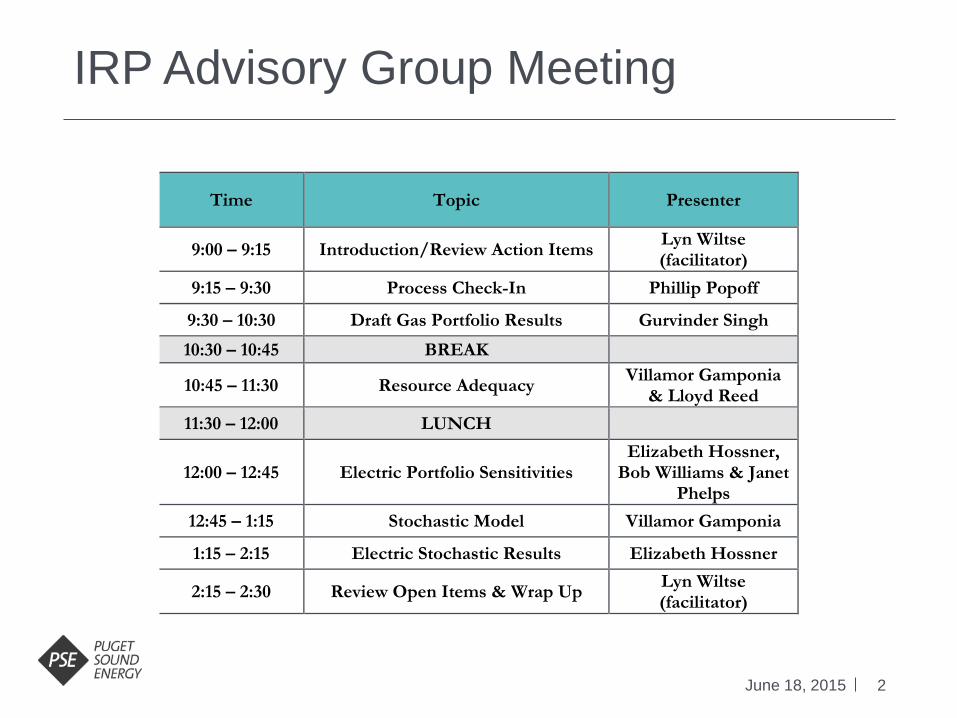
IRP Advisory Group Meeting
June 18, 2015
Time Topic Presenter
9:00 – 9:15 Introduction/Review Action Items Lyn Wiltse (facilitator)
9:15 – 9:30 Process Check-In Phillip Popoff
9:30 – 10:30 Draft Gas Portfolio Results Gurvinder Singh
10:30 – 10:45 BREAK
10:45 – 11:30 Resource Adequacy Villamor Gamponia
& Lloyd Reed
11:30 – 12:00 LUNCH
12:00 – 12:45 Electric Portfolio Sensitivities Elizabeth Hossner,
Bob Williams & Janet Phelps
12:45 – 1:15 Stochastic Model Villamor Gamponia
1:15 – 2:15 Electric Stochastic Results Elizabeth Hossner
2:15 – 2:30 Review Open Items & Wrap Up Lyn Wiltse (facilitator)

Gas Portfolio Analysis Gurvinder Singh
June 18, 2015 IRPAG
4
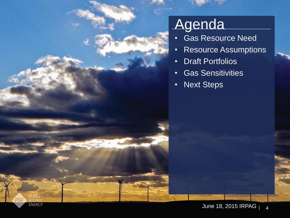
• Gas Resource Need
• Resource Assumptions
• Draft Portfolios
• Gas Sensitivities
• Next Steps
June 18, 2015 IRPAG
Agenda

5
IRP Process
June 18, 2015 IRPAG
Resource Needs
Planning Assumptions &
Resource Alternatives
Analysis of Alternatives
Portfolio Analysis
Analysis of Results
Decisions
Commitment to “Action”

6
2015 IRP - December Peak Day Need Before
DSR
June 18, 2015 IRPAG

7
Supply Side Resource Alternatives
June 18, 2015 IRPAG
Option #1 – Purchase BC gas at Station 2 and transport via existing or expanded
capacity on Westcoast, along with an expansion of Northwest Pipeline (NWP).
Option #1a – Purchase short term NWP TF-1 capacity from Sumas (2016-18)
Option #2 – Purchase AECO gas and transport via existing or expanded capacity on
NGTL (Nova) and Foothills pipelines, along with the proposed Fortis BC Kingsvale -Oliver
Reinforcement Project (KORP) and a NWP expansion.
Option #3 – Purchase AECO gas and transport via existing or expanded capacity on
NGTL, Foothills, GTN, along with a new Cross-Cascades pipeline with a NWP expansion.
(N-MAX, Palomar/Blue Bridge).
Option #4 – Purchase gas at Malin, transport by back-haul on GTN and transport on a
new Cross-Cascades pipeline with a NWP expansion.
Option #5 – Develop an on-system LNG peaking resource in combination with a plant
serving transportation market.
Option #6 – Develop a stand-alone on-system LNG peaking resource MIST Storage –
lease capacity from NW Natural with discounted redelivery to PSE Service territory.
Option #7 – Upgrade the existing Swarr LP-air facility and return to service.

8
Supply Side Resource Alternatives
June 18, 2015 IRPAG

9
Demand Side Resource Alternatives -
Energy
June 18, 2015 IRPAG
Includes 10%
conservation
credit
10
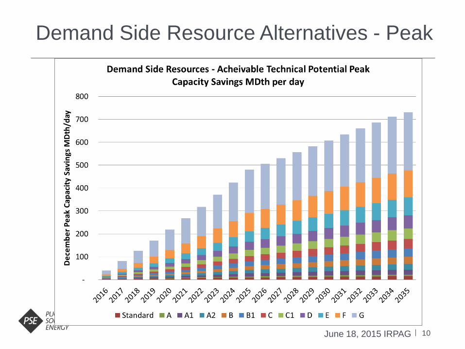
Demand Side Resource Alternatives - Peak
June 18, 2015 IRPAG
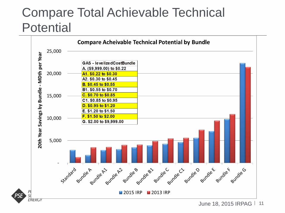
11
Compare Total Achievable Technical
Potential
June 18, 2015 IRPAG

12
Gas Prices - Sumas
June 18, 2015 IRPAG
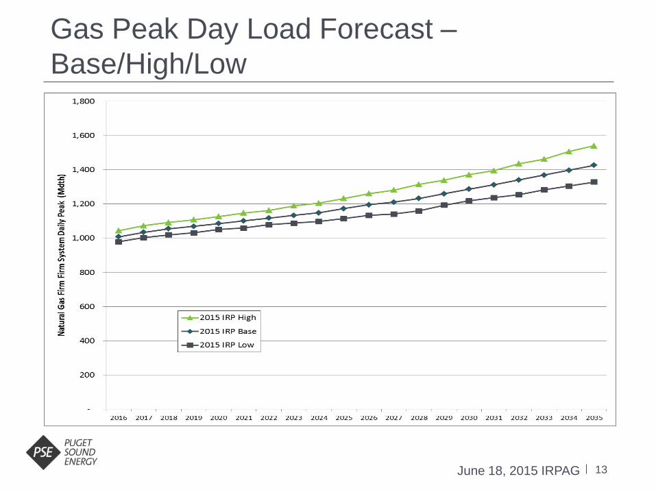
13
Gas Peak Day Load Forecast –
Base/High/Low
June 18, 2015 IRPAG

14
Scenarios
Gas
CO2
Demand
Mid Gas
Mid CO2
Mid Demand
Gas
CO2
Demand
Low
Gas
High
Gas
No
CO2
High
CO2
Low
Demand High
Demand One-Off
Scenarios
Fully Integrated
Scenarios
Very
High
Gas
1
2
3
4
5
6
7 8
9 10
June 18, 2015
IRPAG

15
2015 IRP Scenarios
June 18, 2015 IRPAG
Scenario Demand Gas Price CO2 Price
1 Low Low Low None
2 Base Mid Mid Mid
3 High High High High
4 Base + Low Gas Price Mid Low Mid
5 Base + High Gas Price Mid High Mid
6 Base + Very High Gas Price Mid Very High Mid
7 Base + No CO2 Mid Mid None
8 Base + High CO2 Mid Mid High
9 Base + Low Demand Low Mid Mid
10 Base + High Demand High Mid Mid

16
2015 IRP Gas Sensitivities
June 18, 2015 IRPAG
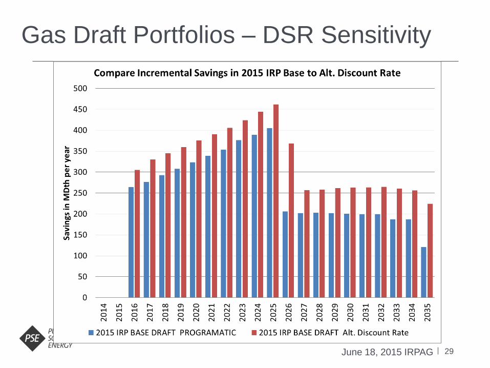
• Compare Cost-effective DSR using alternate discount rate
versus the WACC.
• Developed an alternate weighted discount rate using long term T-bill
and WACC (DSR TAG Meeting April 7th 2014)
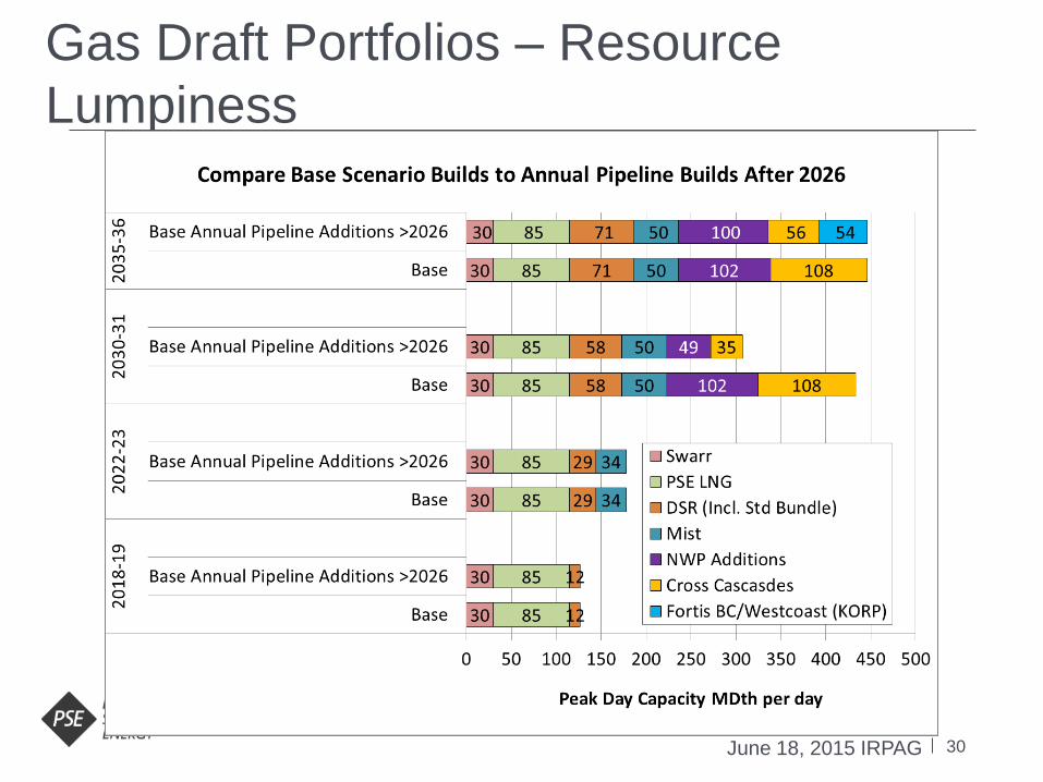
• Test “lumpiness” of pipeline capacity timing:
• “In the next IRP, PSE should conduct a second run of its model once
the appropriate blocks of pipeline capacity are selected, to assess
whether early acquisition of pipeline blocks impacts the timing of the
selection of other resources.” -- Attachment A Utilities and Transportation Commission Comments on Puget
Sound Energy’s 2013 Integrated Resource Plan Dockets UE-120767 & UG-
120768 Section IV Natural Gas page 10.
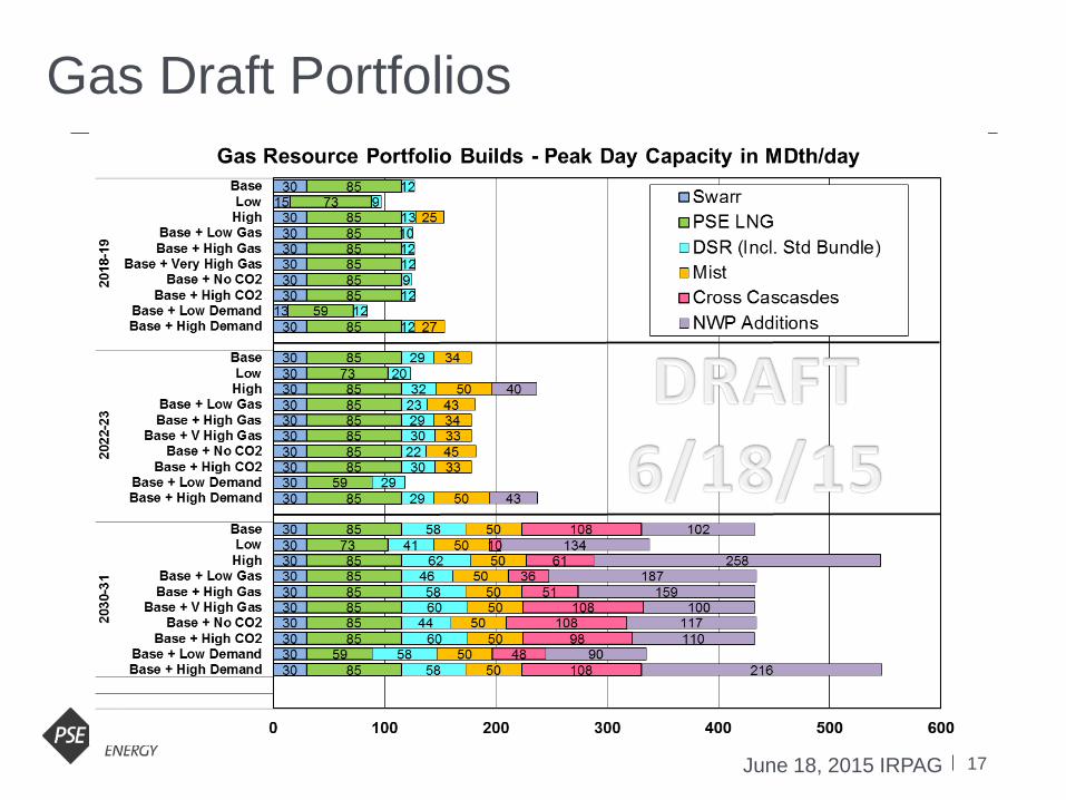
17
Gas Draft Portfolios
June 18, 2015 IRPAG

18
Gas Draft Portfolios - Base Scenario
June 18, 2015 IRPAG

19
Gas Draft Portfolios – DSR Results
June 18, 2015 IRPAG
Bundles Low
2015 IRP
Base High
Base +
Low Gas
Base +
High Gas
Base + V
High Gas
Base + No
CO2
Base +
High CO2
Base +
Low
Demand
Base +
High
Demand
Residential Firm B1 C1 D C1 C1 D C D C1 C1
Commercial Firm B1 D E C D D C D D D
Commercial Interruptible 0 0 0 0 0 0 0 0 0 0
Industrial Firm A2 A2 A2 A2 A2 A2 A2 A2 A2 A2
Industrial Interruptible A2 A2 A2 A2 A2 A2 A2 A2 A2 A2

20
Gas Draft Portfolios – DSR Results
June 18, 2015 IRPAG
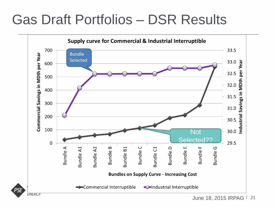
21
Gas Draft Portfolios – DSR Results
June 18, 2015 IRPAG
Not
Selected??

22
Gas Draft Portfolios – DSR Peak
June 18, 2015 IRPAG
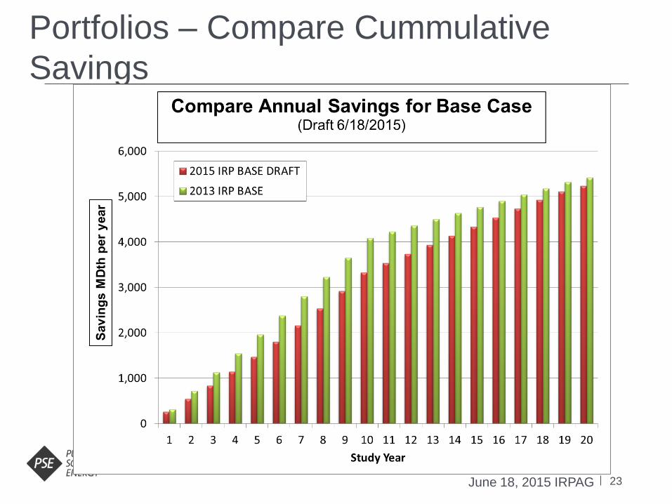
23
Portfolios – Compare Cummulative
Savings
June 18, 2015 IRPAG
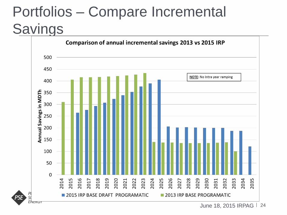
24
Portfolios – Compare Incremental
Savings
June 18, 2015 IRPAG

25
Portfolios – Incremental Codes &
Standards
June 18, 2015 IRPAG
• Water Heater
Standards in 2015 IRP
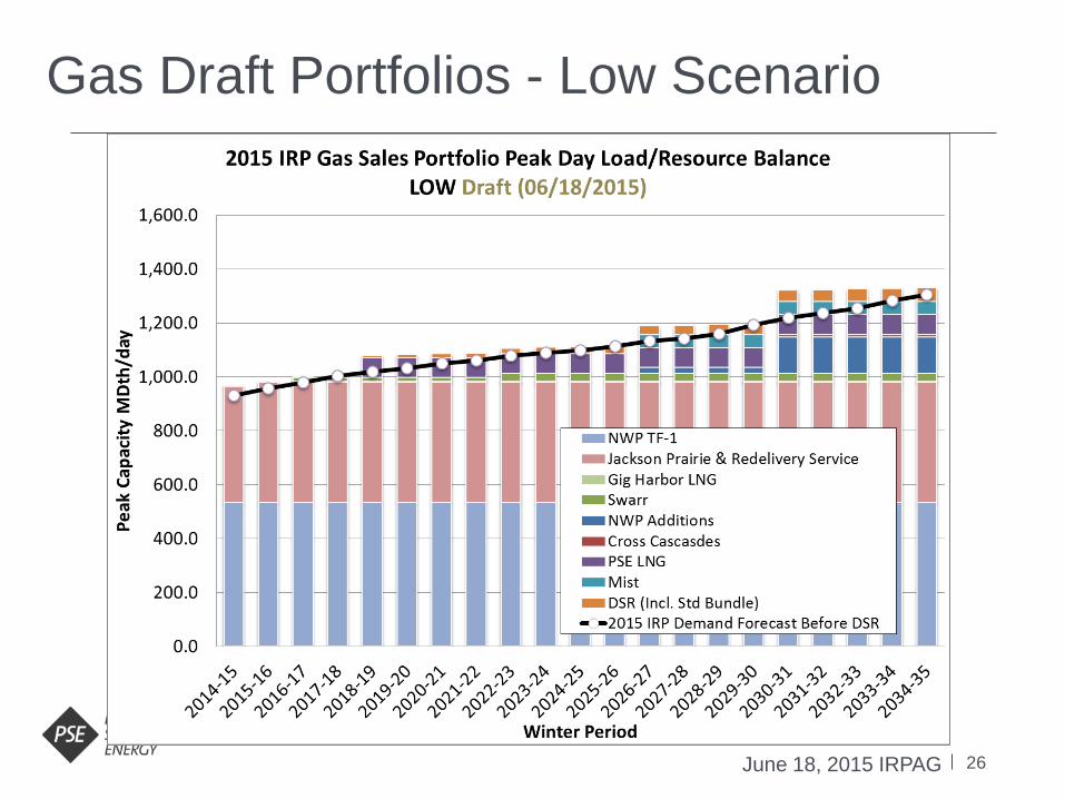
26
Gas Draft Portfolios - Low Scenario
June 18, 2015 IRPAG
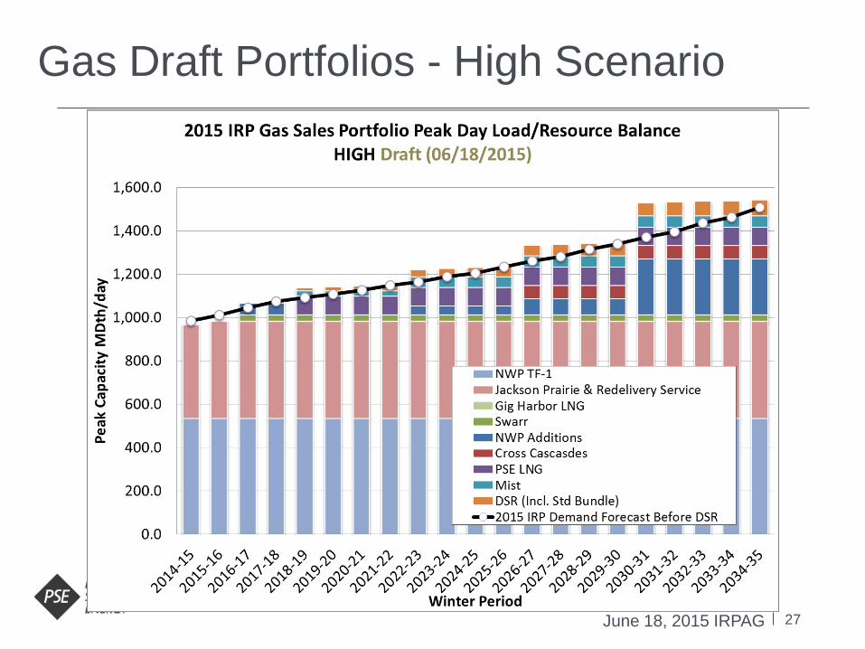
27
Gas Draft Portfolios - High Scenario
June 18, 2015 IRPAG

28
Gas Draft Portfolios – DSR Sensitivity
June 18, 2015 IRPAG
Composite Discount Rate =
Residential Savings Share*Average 3 month of LT CMT + C&I Savings Share*WACC
2014-15 Bienial TargetsSector Therms Percent
Residential 4,020,500 58%
Commercial & Industrial 2,920,000 42%
WACC 7.77%
Ave 3 Month LT CM 30 Yr 2.87%
Composite Discount Rate 4.93%
Dec 09,2014;
Rate as of Jun
17, 2015 is
3.09%
29
Gas Draft Portfolios – DSR Sensitivity
June 18, 2015 IRPAG
30
Gas Draft Portfolios – Resource
Lumpiness
June 18, 2015 IRPAG
31
Gas Draft Portfolios – Resource
Lumpiness
June 18, 2015 IRPAG
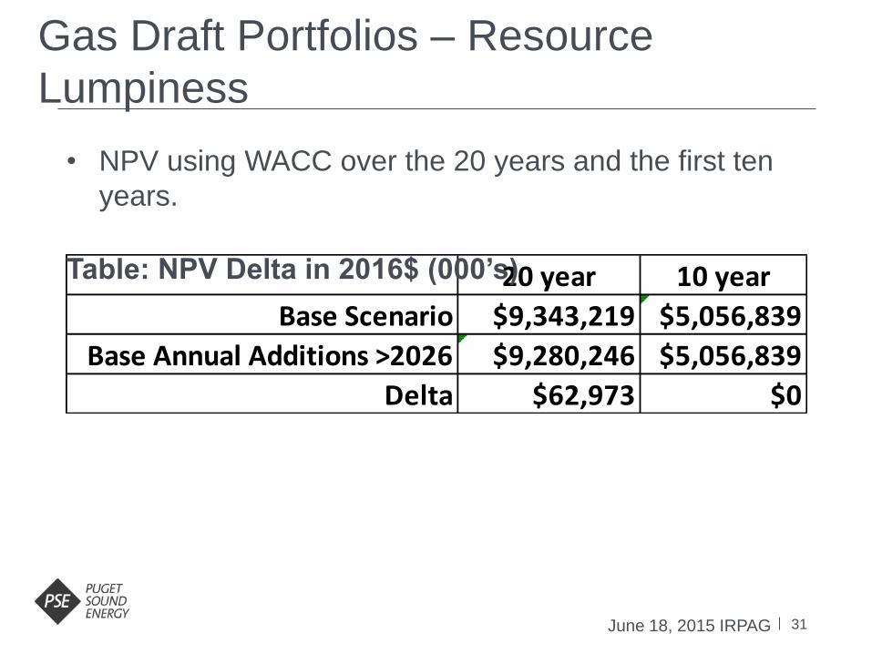
20 year 10 year
Base Scenario $9,343,219 $5,056,839
Base Annual Additions >2026 $9,280,246 $5,056,839
Delta $62,973 $0
• NPV using WACC over the 20 years and the first ten
years.
Table: NPV Delta in 2016$ (000’s)

32
Next Steps
June 18, 2015 IRPAG
• Analyze the portfolio results
• Complete Monte Carlo Analysis
• Gas for Power Portfolio

PSE’s Market Reliance
and Resource Adequacy Villamor Gamponia and Lloyd Reed
June 18, 2015

34
Agenda:
June 18, 2015
PSE’s resource adequacy in the presence of risks in
market reliance
Analytical approach used
Genesys – PNW Resource Adequacy Model
PSE’s Wholesale Purchase Curtailment Model (WPCM)
PSE’s Resource Adequacy Model (RAM)
Impacts of risks in market reliance on PSE’s resource
adequacy
Risk metrics
Benefits and costs of reliability to customers
35
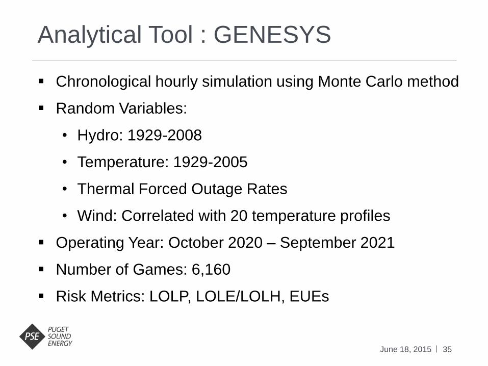
Analytical Tool : GENESYS
June 18, 2015
Chronological hourly simulation using Monte Carlo method
Random Variables:
• Hydro: 1929-2008
• Temperature: 1929-2005
• Thermal Forced Outage Rates
• Wind: Correlated with 20 temperature profiles
Operating Year: October 2020 – September 2021
Number of Games: 6,160
Risk Metrics: LOLP, LOLE/LOLH, EUEs
36
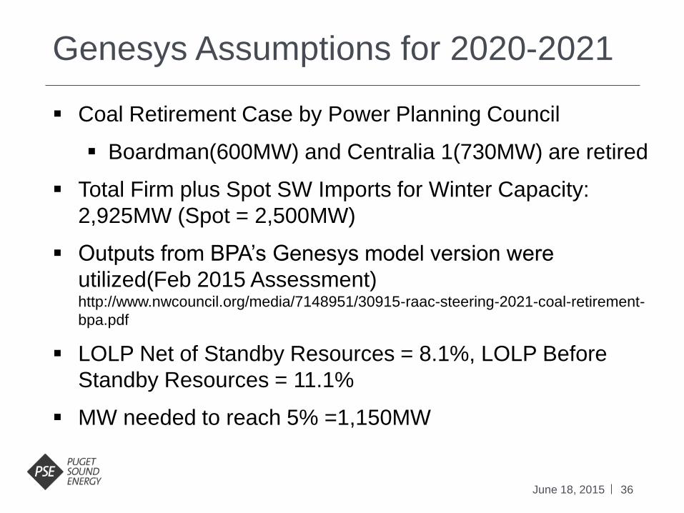
Genesys Assumptions for 2020-2021
June 18, 2015
Coal Retirement Case by Power Planning Council
Boardman(600MW) and Centralia 1(730MW) are retired
Total Firm plus Spot SW Imports for Winter Capacity:
2,925MW (Spot = 2,500MW)
Outputs from BPA’s Genesys model version were
utilized(Feb 2015 Assessment) http://www.nwcouncil.org/media/7148951/30915-raac-steering-2021-coal-retirement-
bpa.pdf
LOLP Net of Standby Resources = 8.1%, LOLP Before
Standby Resources = 11.1%
MW needed to reach 5% =1,150MW

37
Genesys Assumptions for 2020-2021
June 18, 2015
The average PNW load curtailment (in the Genesys draws with curtailments) is 1,950 MW.
The hourly PNW load curtailments from the Genesys model range from 0.2 MW to 10,133 MW.
The maximum hourly PNW curtailment used in the PSE studies was limited to 6,000 MW.
Allocation of Regional Deficits
to PSE Lloyd Reed
External Consultant
June 18, 2015
39
Today’s Topics
June 18, 2015
Introduction/Background
Need for PSE’s Wholesale Purchase Curtailment
Model (WPCM)
WPCM Data Inputs and Assumptions
WPCM Results
WPCM Model Output/Links to Other PSE IRP models
Questions/Discussion

40
Introduction/Background
June 18, 2015
PSE’s 2013 IRP assumed an infinite supply of power is available for PSE to purchase in the PNW wholesale markets under all conditions.
PSE needs to purchase up to approximately 1,600 MW of wholesale capacity and energy to meet its winter season peak load needs.
The changing load/resource situation in the PNW could lead to potential shortages in capacity and energy being available for purchase by PSE and other PNW load-serving utilities.
Over 2,000 MW of regional coal-fired generation will be retired by 2025.
PSE’s wholesale purchases could be limited to amounts significantly less than 1,600 MW during PNW regional load curtailment events.
Key Question: How can the impacts of PNW regional load curtailment events be quantified and included in PSE’s 2015 IRP resource adequacy analysis?

41
Need for PSE’s Wholesale Purchase Curtailment Model
June 18, 2015
PNW Resource Adequacy studies performed by the NWPCC and BPA
are conducted on an aggregated region-wide basis.
It is not possible to isolate on impacts to individual utilities.
Lack of other available modeling tools to translate PNW-wide regional
load curtailments to an individual utility level.
No PNW IOU attempted to quantify potential regional load curtailment
impacts in their respective 2013 IRPs.
Conclusion: PSE needs to develop a new modeling tool for use in the
2015 IRP to quantify the impacts of PNW-wide load curtailment events
on PSE’s power system.
Impacts will be quantified via reductions in PSE’s wholesale market
purchases under its long-term Mid-C transmission rights.
42
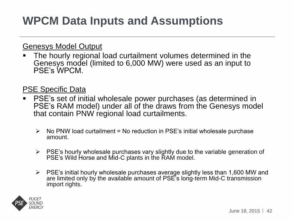
WPCM Data Inputs and Assumptions
June 18, 2015
Genesys Model Output
The hourly regional load curtailment volumes determined in the Genesys model (limited to 6,000 MW) were used as an input to PSE’s WPCM.
PSE Specific Data
PSE’s set of initial wholesale power purchases (as determined in PSE’s RAM model) under all of the draws from the Genesys model that contain PNW regional load curtailments.
No PNW load curtailment = No reduction in PSE’s initial wholesale purchase
amount.
PSE’s hourly wholesale purchases vary slightly due to the variable generation of PSE’s Wild Horse and Mid-C plants in the RAM model.
PSE’s initial hourly wholesale purchases average slightly less than 1,600 MW and are limited only by the available amount of PSE’s long-term Mid-C transmission import rights.

43
WPCM Data Inputs and Assumptions (Cont.)
June 18, 2015
PNW Regional Load/Resource Data
The surplus/deficit position of other PNW utilities has a direct impact on the amount of PNW-wide load curtailments that are ultimately “allocated” to PSE.
Load and resource data for 2021 was compiled from various sources to determine the net winter capacity surplus or deficiency for multiple PNW utilities.
2013 IRPs for PGE, Pacificorp, Avista and Idaho Power.
BPA’s 2014 Pacific Northwest Loads and Resources Study.
Other forecasted 2021 large PNW purchasers of winter capacity (relative to PSE) include PGE, Pacificorp (West System) and BPA.
Aggregating small capacity purchasers and sellers does not impact the PSE load curtailment allocations.

44
WPCM Data Inputs and Assumptions (Cont.)
June 18, 2015
Load and resource data was used to compute winter 2021 base capacity surplus/(deficiencies) for the above noted utilities, BPA’s public preference customers by category (i.e. PUDs, municipalities, etc.), PNW regional IPPs, and power marketers.
Sensitivities to changes in regional load and resource conditions were determined based upon each entity’s total winter peak load + winter peaking resources. Sensitivity ratios were utilized to sync up the base individual utility
surplus/(deficiencies) to the hourly PNW regional load curtailment amounts from the Genesys model.
The base PNW winter 2021 capacity surpluses/(deficiencies) and sensitivity ratios utilized in the PSE WPCM model are shown in the following table:

45
WPCM Data Inputs and Assumptions (Cont.)
June 18, 2015
PNW Entity Base 2021 Winter Capacity Surplus/(Deficiencies) and
Sensitivity Ratios
Entity Sur/(Def) Sensitivity
MW Ratios
PSE (1,584.1) 0.15
PGE (789.0) 0.11
PACW (1,175.9) 0.11
BPA (797.0) 0.30
Other (635.0) 0.21
PNW IPP+IPC 3,188.0 0.12
Total (1,793.0) 1.00
46
WPCM Data Inputs and Assumptions (Cont.)
June 18, 2015
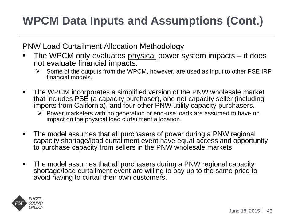
PNW Load Curtailment Allocation Methodology
The WPCM only evaluates physical power system impacts – it does not evaluate financial impacts. Some of the outputs from the WPCM, however, are used as input to other PSE IRP
financial models.
The WPCM incorporates a simplified version of the PNW wholesale market that includes PSE (a capacity purchaser), one net capacity seller (including imports from California), and four other PNW utility capacity purchasers. Power marketers with no generation or end-use loads are assumed to have no
impact on the physical load curtailment allocation.
The model assumes that all purchasers of power during a PNW regional capacity shortage/load curtailment event have equal access and opportunity to purchase capacity from sellers in the PNW wholesale markets.
The model assumes that all purchasers during a PNW regional capacity shortage/load curtailment event are willing to pay up to the same price to avoid having to curtail their own customers.

47
WPCM Data Inputs and Assumptions (Cont.)
June 18, 2015
The model incorporates impacts from both forward-market purchases and spot-market purchases. Forward-market purchases are assumed to be initiated well in advance of a PNW
load curtailment event (i.e. under “normal” market conditions).
Spot-market purchases are assumed to be initiated on a day-ahead or day-of basis (i.e. under “non-normal” capacity scarcity conditions).
A utility that manages to purchase more capacity than it needs to meet its own need (i.e. to avoid a load curtailment to its own customers) will make that surplus capacity available to other (still deficit) PNW capacity purchasers.
Under PNW capacity shortage/load curtailment events, BOTH forward-market wholesale purchases and spot-market wholesale purchases could be subject to curtailment. In general, forward-market purchases do not have a priority over spot-market
purchases.
It is in the seller’s discretion as to which wholesale sales it may choose to curtail if required.
48
WPCM Results
June 18, 2015
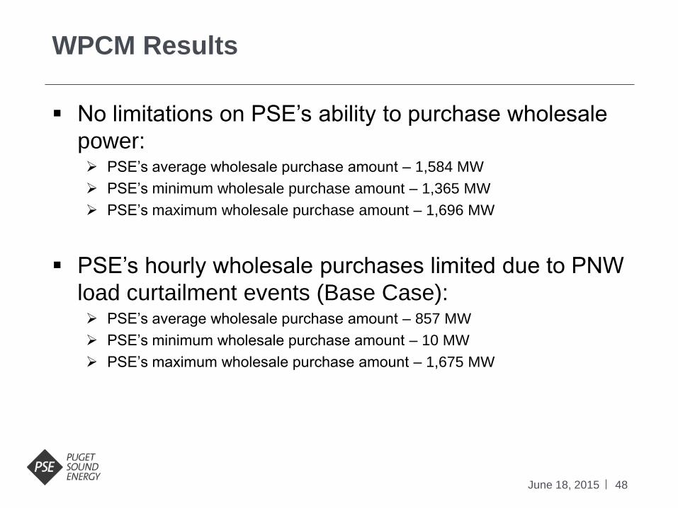
No limitations on PSE’s ability to purchase wholesale
power: PSE’s average wholesale purchase amount – 1,584 MW
PSE’s minimum wholesale purchase amount – 1,365 MW
PSE’s maximum wholesale purchase amount – 1,696 MW
PSE’s hourly wholesale purchases limited due to PNW
load curtailment events (Base Case): PSE’s average wholesale purchase amount – 857 MW
PSE’s minimum wholesale purchase amount – 10 MW
PSE’s maximum wholesale purchase amount – 1,675 MW

49
WPCM Model Output/Links to Other PSE IRP models
June 18, 2015
For each hourly PNW load curtailment event (as determined in the
Genesys model) the primary outputs from the WPCM model are:
PSE’s initial hourly wholesale market purchase (in MW).
The reduction to PSE’s initial hourly wholesale market purchase that
incorporates the PNW load curtailment/capacity scarcity event (in MW).
PSE’s final hourly wholesale market purchase (in MW).
The final set of PSE hourly wholesale market purchases in then used
as an input into the second and final run of PSE’s RAM model.
PNW load curtailment impacts on PSE across the 6,160 Genesys
draws are “translated” to the 250 draw datasets that are utilized in
the PSE financial models.
Wholesale power prices are adjusted in PSE’s IRP financial models to
incorporate PNW regional scarcity pricing impacts.
50
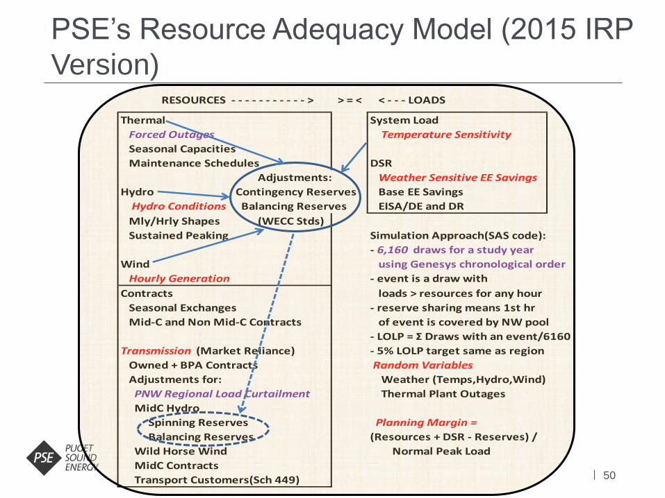
PSE’s Resource Adequacy Model (2015 IRP
Version) > = <
Thermal System Load
Forced Outages Temperature Sensitivity
Seasonal Capacities
Maintenance Schedules DSR
Adjustments: Weather Sensitive EE Savings
Hydro Contingency Reserves Base EE Savings
Hydro Conditions Balancing Reserves EISA/DE and DR
Mly/Hrly Shapes (WECC Stds)
Sustained Peaking Simulation Approach(SAS code):
- 6,160 draws for a study year
Wind using Genesys chronological order
Hourly Generation - event is a draw with
Contracts loads > resources for any hour
Seasonal Exchanges - reserve sharing means 1st hr
Mid-C and Non Mid-C Contracts of event is covered by NW pool
- LOLP = Ʃ Draws with an event/6160
Transmission (Market Reliance) - 5% LOLP target same as region
Owned + BPA Contracts Random Variables
Adjustments for: Weather (Temps,Hydro,Wind)
PNW Regional Load Curtailment Thermal Plant Outages
MidC Hydro
Spinning Reserves Planning Margin =
Balancing Reserves (Resources + DSR - Reserves) /
Wild Horse Wind Normal Peak Load
MidC Contracts
Transport Customers(Sch 449)
RESOURCES - - - - - - - - - - - > < - - - LOADS

51
PSE’s Resource Adequacy Model (Updates
to the 2015 IRP Version)
June 18, 2015
Based on F14 load forecasts(lower by 120MW in
2020 from F13)
Consistency with Genesys draws:
Same study period: Oct 2020 to Sep 2021
Chronological simulation of weather and temperature
years (Hydro:1929-2008; Temperature: 1929-2005)
Forced outage assumptions for expected FOR and
mean time to repair are the same for PSE thermals
Hourly reductions in market purchase capability
from WPCM in Genesys games with curtailments

52
Reliability Metrics for 2020-2021
June 18, 2015
Planning Margin
@5% LOLP
No Risk in Market Reliance 13%
With Risk in Market Reliance 14%
*Risks in market reliance are based on shortages from the regional adequacy model with coal retirements in 2020.
**For games with any interruption, similar to SAIFI(interruptions)/SAIDI(duration).PSE Targets:SAIFI=1.3,SAIDI=5.33
Risk in market reliance significantly increases the expected unserved
energy or EUE even with added capacity to achieve the same LOLP.

53
Peak Contribution of Wind
June 18, 2015
ICE – Incremental Capacity Equivalents, if we add or subtract a resource,
what level of gas peaking capacity needs to be subtracted or added
respectively to keep the 5% LOLP. The ratio of the change in gas peaking
capacity to the capacity of the new added or subtracted resource gives an
estimate of the peak contribution of a resource.
Incrementa l Capacity Equiva lent(Re la tive to a Peaker)
ICE Va lue
Existing Wind 12.5%
SW WA Generic Wind 7.0%
MT Generic Wind 55.0%
• SW Washington Wind profile is based on historical Hopkins Ridge lagged 10
minutes
• MT Generic Wind profile is based on 2 years of historical Judith Gap wind data
• EUE based incremental capacity equivalent could be different

54
Impacts of Added SW Imports and Resource
Reductions due to Non-Firm Gas Supply
June 18, 2015
No Risk in
Market
Reliance
With Risk in
Market
Reliance*
With Risk in Market
Reliance + Full SW
Import(+475MW)
With Risk in Market Reliance
+ Capacity Drop for Non-
Firm Fuel(-650MW)
LOLP 5% 5% 5% 5%
LOLE/LOLH(Hrs) 0.20 0.25 0.23 0.29
Expected Unserved Energy(MW-Hrs) 26.2 49.6 41.6 61.2
TVar90 of Unserved Energy(MW-Hrs) 262 496 416 612
Exp Number of Interruptions/Year** 1.9 2.0 1.9 2.1
Exp Duration/Interruption(Hrs)** 2.14 2.55 2.45 2.75
* Risks in market reliance are based on shortages from the regional adequacy model
with coal retirements in 2020-2021. Assumes Boardman and Centralia 1 are retired in 2020.
** For games with any interruption, similar to SAIFI(interruptions)/SAIDI(duration).PSE targets:SAIFI=1.3,SAIDI=5.33

55
Market Reliance Risks and Value of Lost Loads
June 18, 2015
Risks in market reliance increase unserved energy and
customer interruptions
Need to evaluate benefits/costs of reliability
Inputs required:
PSE’s Resource Adequacy Model produces system lost
loads by month/day/hour and by duration
Interruption cost estimates per event by customer type
are available from DOE, based on LBL compilation of
surveys(www.icecalculator.com)
Costs of adding a frame peaker to meet reliability is
available from PSM

56
Benefit-Cost of Reliability
57
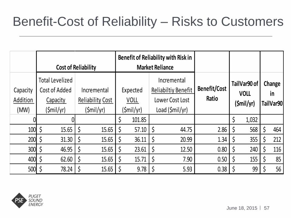
Benefit-Cost of Reliability – Risks to Customers
June 18, 2015
Capacity
Addition
(MW)
Total Levelized
Cost of Added
Capacity
($mil/yr)
Incremental
Reliability Cost
($mil/yr)
Expected
VOLL
($mil/yr)
Incremental
Reliabiltiy Benefit
Lower Cost Lost
Load ($mil/yr)
Benefit/Cost
Ratio
TailVar90 of
VOLL
($mil/yr)
Change
in
TailVar90
0 0 101.85$ 1,032$
100 15.65$ 15.65$ 57.10$ 44.75$ 2.86 568$ 464$
200 31.30$ 15.65$ 36.11$ 20.99$ 1.34 355$ 212$
300 46.95$ 15.65$ 23.61$ 12.50$ 0.80 240$ 116$
400 62.60$ 15.65$ 15.71$ 7.90$ 0.50 155$ 85$
500 78.24$ 15.65$ 9.78$ 5.93$ 0.38 99$ 56$
Cost of Reliability
Benefit of Reliability with Risk in
Market Reliance

Electric Portfolio Analysis
Elizabeth Hossner
June 18, 2015 IRPAG

59
Draft Portfolio Builds - Base
June 18, 2015 IRPAG
Annual
Builds (MW) CCCT
Frame
Peaker WA Wind Biomass PBA Battery DSR DR
2016 - - - - - - 75 18
2017 - - - - - - 64 12
2018 - - - - - - 67 41
2019 - - - - - - 64 14
2020 - - - - - - 79 43
2021 - - - - - - 62 2
2022 - - - - 25 - 66 12
2023 - 228 100 - - - 56 2
2024 - - 100 - - - 55 3
2025 - - - - - - 53 2
2026 - 455 - - - - 27 2
2027 - - 100 - - - 27 2
2028 - 228 - - - - 27 3
2029 - - - - - - 23 2
2030 - - - - - - 23 2
2031 - 228 - - - - 27 2
2032 - - - - - - 32 2
2033 - - - 15 - - 29 2
2034 - - - - - - 25 2
2035 - - - - - 80 24 2
Total - 1,138 300 15 25 80 906 172
Winter - 1,138 24 - 25 80 906 172

60
Meeting Peak Capacity - Base
-
1,000
2,000
3,000
4,000
5,000
6,000
7,000
8,000
9,000
2016 2017 2018 2019 2020 2021 2022 2023 2024 2025 2026 2027 2028 2029 2030 2031 2032 2033 2034 2035
Pe
ak C
apac
ity
(MW
)
Demand Side Resources
Fixed PPA
Batteries
MT Wind
Solar
Biomass
WA Wind
Peaker - Recip
Peaker - Aero
Peaker - Frame
CCGT
Mid-C Transmission Available
Existing Resources (full capacity)
Dec Peak Load + PM + Op Reserves

61
Meeting RPS - Base
June 18, 2015 IRPAG
0
500
1000
1500
2000
2500
3000
3500
4000
2016 2017 2018 2019 2020 2021 2022 2023 2024 2025 2026 2027 2028 2029 2030 2031 2032 2033 2034 2035
Tota
l REC
s G
Wh
Meeting the RPS
Generic Solar
Generic MT Wind
Generic Biomass
Generic WA Wind
Hydro Upgrades
Existing Resources
REC Need ('000)
62
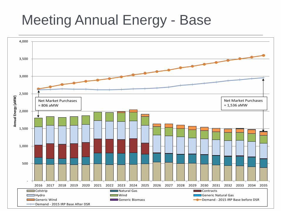
Meeting Annual Energy - Base
-
500
1,000
1,500
2,000
2,500
3,000
3,500
4,000
2016 2017 2018 2019 2020 2021 2022 2023 2024 2025 2026 2027 2028 2029 2030 2031 2032 2033 2034 2035
Ann
ual E
nerg
y (a
MW
)
Colstrip Natural Gas Contracts
Hydro Wind Generic Natural Gas
Generic Wind Generic Biomass Demand - 2015 IRP Base before DSR
Demand - 2015 IRP Base After DSR
Net Market Purchases = 806 aMW
Net Market Purchases = 1,536 aMW
63
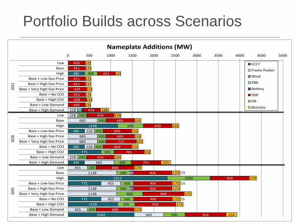
Portfolio Builds across Scenarios
385
1156
385
385
771
385
2312
771
771
1156
1542
228
228
683
228
683
683
228
228
683
455
1138
455
1138
1138
455
455
683
300
200
200
600
200
200
200
200
300
200
400
200
300
1000
300
300
600
300
400
200
500
100
80
80
403
411
411
411
411
435
411
428
403
428
654
669
669
669
669
713
669
701
654
701
888
906
906
906
906
968
906
956
888
956
131
131
131
131
131
131
131
131
131
198
154
152
154
152
152
152
152
152
154
225
174
172
174
172
172
172
172
172
174
254
15
15
15
0 500 1000 1500 2000 2500 3000 3500 4000 4500 5000
Low
Base
High
Base + Low Gas Price
Base + High Gas Price
Base + Very High Gas Price
Base + No CO2
Base + High CO2
Base + Low Demand
Base + High Demand
Low
Base
High
Base + Low Gas Price
Base + High Gas Price
Base + Very High Gas Price
Base + No CO2
Base + High CO2
Base + Low Demand
Base + High Demand
Low
Base
High
Base + Low Gas Price
Base + High Gas Price
Base + Very High Gas Price
Base + No CO2
Base + High CO2
Base + Low Demand
Base + High Demand
2021
2026
2035
Nameplate Additions (MW)
CCCT
Frame Peaker
Wind
PBA
Battery
DSR
DR
Biomass

64
Draft Portfolios – Portfolio Sensitivities

65
Portfolio Sensitivities
June 18, 2015 IRPAG
Sensitivities Alternatives Analyzed
A Market Reliance Risk
What if continuing to rely on short-term market purchases becomes too risky?
Baseline – Continue to rely on 1,600 MW of
market purchases
1.
B Gas Transport for Peakers
What if peakers cannot rely on oil for
backup fuel and must have firm gas supply instead?
Baseline – Non-firm pipeline capacity with oil
backup
2. Firm pipeline capacity with no oil backup
C Solar Penetration
What if customers install significantly more rooftop solar than expected?
Baseline – Rooftop solar growth based on
forecast
3. Maximum potential capture of rooftop solar

66
Portfolio Sensitivities Continued
June 18, 2015 IRPAG
Sensitivities Alternatives Analyzed
D Energy Storage/Flexible Resource
What is the cost difference between a
portfolio with and without and energy storage or Flexible Resource?
Baseline – Batteries economically chosen as
part of least cost portfolio
4. Add 80 MW Battery in 2023 instead of Peaker
5. Add 80 MW Pumped Storage Hydro in 2023
instead of Peaker
6. Update Costs for Recip Engine (75 MW)
7. Add 75 MW Recip Engine in 2023 E Demand-side Resources (DSR)
How much does DSR reduce cost, cost risk and emissions?
Baseline – All cost-effective DSR per RCW
19.285 requirements
8. No DSR. All needs met with supply-side resources
F Carbon Reduction
How does increasing renewable resources
and DSR beyond requirements affect carbon reduction and portfolio costs?
Baseline – Renewable resources and DSR per
RCW 19.285 requirements
9. Add 300 MW of wind in 2021 beyond
renewable requirements
10. Add 300 MW of utility scale solar in 2021
beyond renewable requirements
11. DSR increased beyond requirements
67
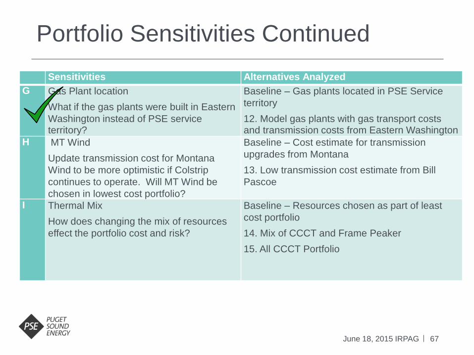
Portfolio Sensitivities Continued
June 18, 2015 IRPAG
Sensitivities Alternatives Analyzed
G Gas Plant location
What if the gas plants were built in Eastern
Washington instead of PSE service territory?
Baseline – Gas plants located in PSE Service
territory
12. Model gas plants with gas transport costs and transmission costs from Eastern Washington
H MT Wind
Update transmission cost for Montana
Wind to be more optimistic if Colstrip
continues to operate. Will MT Wind be
chosen in lowest cost portfolio?
Baseline – Cost estimate for transmission
upgrades from Montana
13. Low transmission cost estimate from Bill
Pascoe
I Thermal Mix
How does changing the mix of resources
effect the portfolio cost and risk?
Baseline – Resources chosen as part of least
cost portfolio
14. Mix of CCCT and Frame Peaker
15. All CCCT Portfolio
68
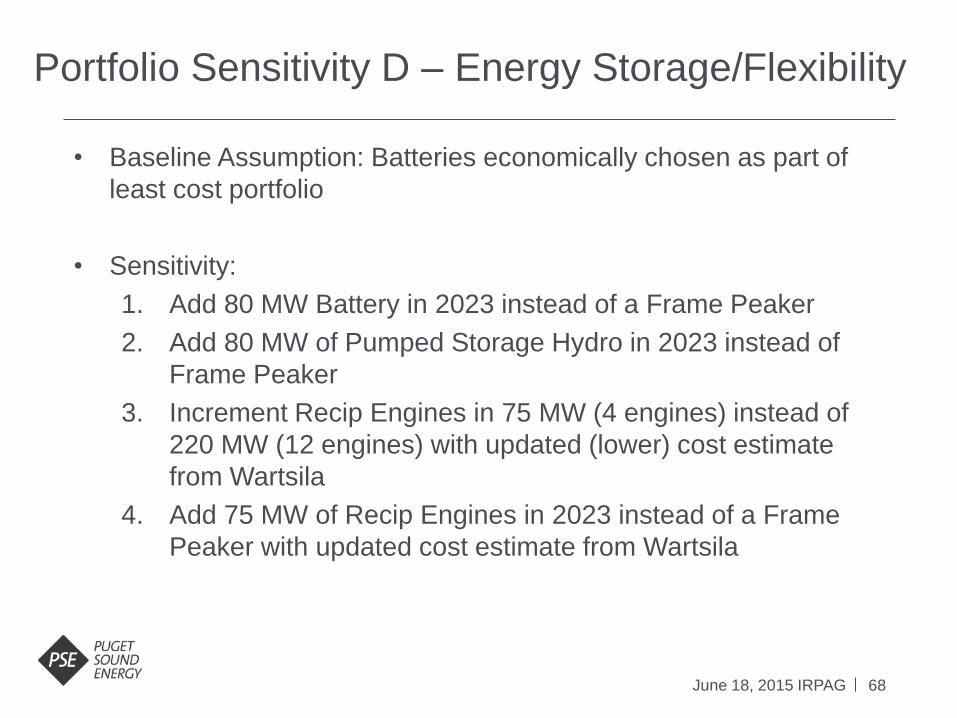
Portfolio Sensitivity D – Energy Storage/Flexibility
June 18, 2015 IRPAG
• Baseline Assumption: Batteries economically chosen as part of
least cost portfolio
• Sensitivity:
1. Add 80 MW Battery in 2023 instead of a Frame Peaker
2. Add 80 MW of Pumped Storage Hydro in 2023 instead of
Frame Peaker
3. Increment Recip Engines in 75 MW (4 engines) instead of
220 MW (12 engines) with updated (lower) cost estimate
from Wartsila
4. Add 75 MW of Recip Engines in 2023 instead of a Frame
Peaker with updated cost estimate from Wartsila

69
Portfolio Sensitivity D – Recip Assumptions
June 18, 2015 IRPAG
Updated costs on Reciprocating Engines from Wartsila. Cost estimates provided by Burns and McDonnell for a plant in the Seattle/PSE area.
Current EPC estimate for a 18V50SG (18.7 MW each):
4 x 18V50SG (74.8 MW): $72 million ($962/KW)
6 x 18V50SG (112.2 MW): $95.4 million ($850/KW)
10 x 18V50SG (187 MW): $152 million ($812/KW)
Assumptions:
• Air-cooled radiators installed on the ground
• No piles required for foundations
• SCR included
• Separate contracts for Wartsila gensets and engineering/construction
• Does not include cost of transmission interconnect
PSE adds 40% for outside-the-fence, project development, project financing, and escalation
70
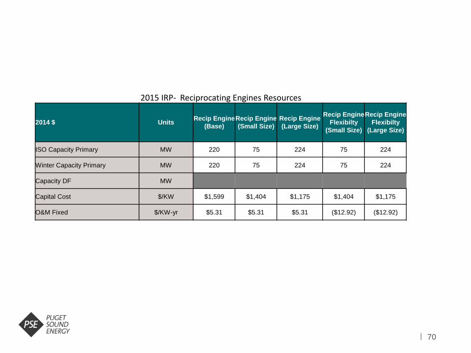
2015 IRP- Reciprocating Engines Resources
2014 $ Units Recip Engine
(Base)
Recip Engine
(Small Size)
Recip Engine
(Large Size)
Recip Engine
Flexibilty
(Small Size)
Recip Engine
Flexibilty
(Large Size)
ISO Capacity Primary MW 220 75 224 75 224
Winter Capacity Primary MW 220 75 224 75 224
Capacity DF MW
Capital Cost $/KW $1,599 $1,404 $1,175 $1,404 $1,175
O&M Fixed $/KW-yr $5.31 $5.31 $5.31 ($12.92) ($12.92)

71
Portfolio
CPS2
Score
Proxy
(%)*
Spin
Capacity
Shortfall
(%)
Spin
Capacity
Shortfall
(aMW)
Unserved
Energy
(aMW)
Excess
Energy
(aMW)
Expected
Annual
Balancing
Savings
($)
Expected
Annual
Bal.
Savings
($/kW
Capacity)
2018 Base 97% 0.1% 2.0 5.9 12.5 -- --
2018 Base +
CCCT 97% 0.1% 1.8 5.7 12.2 $800,000 $2.33
2018 Base +
Frame CT 97% 0.1% 1.9 5.9 12.1 $1,037,000 $4.69
2018 Base +
Recip CT 97% 0.1% 1.8 5.9 12.1 $328,000 $18.23
Figure G-13
Summary Results from Flexibility Analysis,
50 Simulations
APPENDIX G – OPERATIONAL FLEXIBILITY
Source: 2013 IRP

72
(A) (B) (C) (D) (E)=(A)-(C) (F) (G) (H)=(A)-(G)
Difference
from base
Difference
from base
Difference
from base
Portfolio Costs
Benefit/
(Cost) Portfolio Costs
Benefit/
(Cost)
Value of
Flexibility to
the Portfolio
Portfolio
Costs
Benefit/
(Cost)
Value of
Flexibility to
the Portfolio
Base Case $12,276,911 $12,221,360 $55,551 $12,221,360 $55,551
Reciprocating Engines 75 MW* $12,263,289 $13,622 $12,201,832 $19,528 $61,457 $12,207,549 $13,810 $55,740
Reciprocating Engines 75 MW in 2023 $12,281,901 ($4,990) $12,211,855 $9,504 $70,046 $12,220,589 $770 $61,311
Reciprocating Engine 224 MW in 2023 $12,354,297 ($77,386) $12,234,783 ($13,424) $119,513 $12,260,986 ($39,626) $93,311
*Replaces battery in 2035 as a cheaper alternative
No Flexibility Benefit
Sensitivity of Reciprocating Engines
Flexibility Benefits 50% for RecipsFlexibility Benefits
73
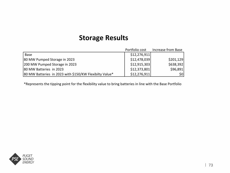
Portfolio cost Increase from Base
Base $12,276,911
80 MW Pumped Storage in 2023 $12,478,039 $201,129
200 MW Pumped Storage in 2023 $12,915,303 $638,392
80 MW Batteries in 2023 $12,373,801 $96,891
80 MW Batteries in 2023 with $150/KW Flexibilty Value* $12,276,911 $0
*Represents the tipping point for the flexibility value to bring batteries in line with the Base Portfolio
Storage Results
74
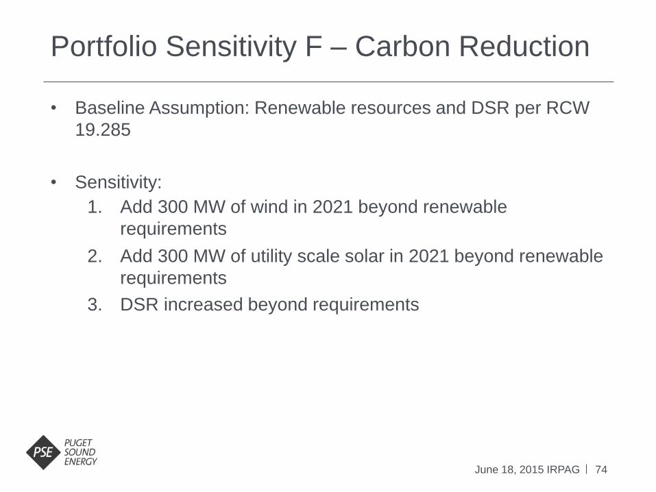
Portfolio Sensitivity F – Carbon Reduction
June 18, 2015 IRPAG
• Baseline Assumption: Renewable resources and DSR per RCW
19.285
• Sensitivity:
1. Add 300 MW of wind in 2021 beyond renewable
requirements
2. Add 300 MW of utility scale solar in 2021 beyond renewable
requirements
3. DSR increased beyond requirements
75
What is the cost of carbon abatement?
June 18, 2015 IRPAG
• Addition of demand side or renewable
resources to portfolio changes revenue
requirement and emissions
• Other elements of portfolio change to
accommodate added resource
76
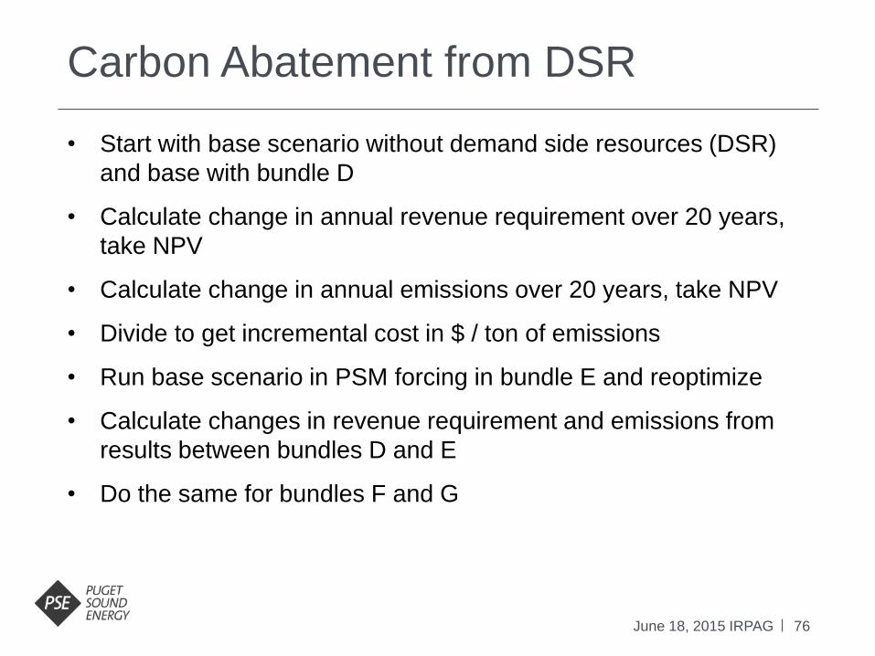
Carbon Abatement from DSR
June 18, 2015 IRPAG
• Start with base scenario without demand side resources (DSR)
and base with bundle D
• Calculate change in annual revenue requirement over 20 years,
take NPV
• Calculate change in annual emissions over 20 years, take NPV
• Divide to get incremental cost in $ / ton of emissions
• Run base scenario in PSM forcing in bundle E and reoptimize
• Calculate changes in revenue requirement and emissions from
results between bundles D and E
• Do the same for bundles F and G

77
Incremental Cost by Bundle
June 18, 2015 IRPAG

78
Carbon Abatement by Bundle
June 18, 2015 IRPAG

79
Impacts of Changing DSR
Changes to portfolio cost and emissions reflect impacts of multiple changes to portfolios. Increments are calculated
relative to portfolio with previous bundle.
Scenario
NPV 20 Year
Portfolio
Cost ($000)
Total 20
Year
Emissions
(Millions of
Tons)
Total 20
Year
Carbon
Abatement
(Millions of
Tons)
Incremental
Cost
(Benefit) /
Ton
Base No DSR $12,339,055 245.00
Base Bundle D $11,019,322 228.89 16.11 $(202)
Bundle E $11,077,321 227.99 0.90 $173
Bundle F $11,075,068 227.74 0.25 $(23)
Bundle G $11,155,377 226.52 1.22 $157
80
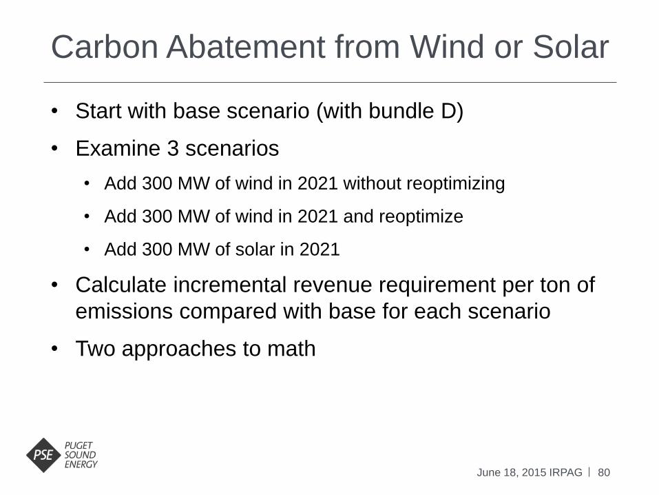
Carbon Abatement from Wind or Solar
June 18, 2015 IRPAG
• Start with base scenario (with bundle D)
• Examine 3 scenarios
• Add 300 MW of wind in 2021 without reoptimizing
• Add 300 MW of wind in 2021 and reoptimize
• Add 300 MW of solar in 2021
• Calculate incremental revenue requirement per ton of
emissions compared with base for each scenario
• Two approaches to math
81
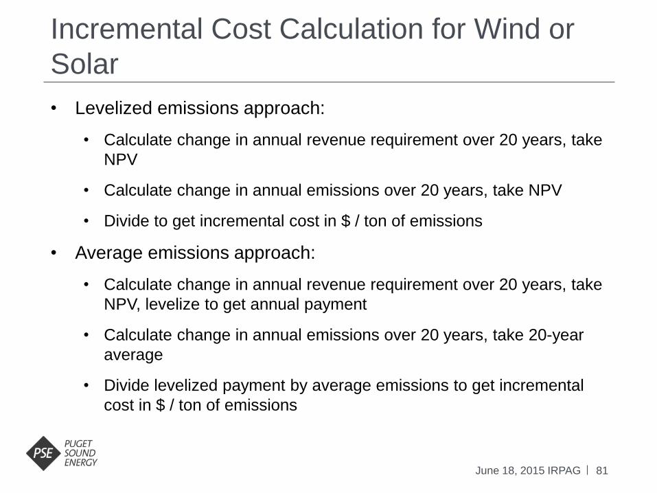
Incremental Cost Calculation for Wind or
Solar
June 18, 2015 IRPAG
• Levelized emissions approach:
• Calculate change in annual revenue requirement over 20 years, take
NPV
• Calculate change in annual emissions over 20 years, take NPV
• Divide to get incremental cost in $ / ton of emissions
• Average emissions approach:
• Calculate change in annual revenue requirement over 20 years, take
NPV, levelize to get annual payment
• Calculate change in annual emissions over 20 years, take 20-year
average
• Divide levelized payment by average emissions to get incremental
cost in $ / ton of emissions

82
Incremental Cost for Wind and Solar
June 18, 2015 IRPAG

83
Carbon Abatement from Wind or Solar
June 18, 2015 IRPAG

84
Impacts of Wind or Solar Additions
June 18, 2015 IRPAG
Changes to portfolio cost and emissions reflect impacts of multiple changes to portfolios. Increments for both wind
and solar are calculated relative to base scenario.
Scenario
NPV 20
Year
Portfolio
Cost ($000)
Total 20
Year
Emissions
(Millions
of Tons)
Total 20
Year
Carbon
Abatement
(Millions
of Tons)
Incremental
Cost
(Benefit) /
Ton
Base Bundle D $11,019,322 228.89
300 MW Wind (Not
Reoptimized)
$11,239,345
223.98
4.91
$115
300 MW Wind
(Reoptimized)
$11,111,563 223.98 4.91 $36 - 38
300 MW Solar $11,423,572 226.11 2.78 $362 - 374

85
Portfolio Sensitivity H – Montana Wind
June 18, 2015 IRPAG
• Baseline Assumption: Cost estimate for transmission upgrades
from Montana
• Sensitivity: Low transmission cost estimate based on
conversations with Bill Pascoe
• Follow-up with Bill on details

86
2014 $ WA Wind MT Wind Base MT Wind Update
Capital Cost Facility ($/kW) $1,703 $1,703 $1,703
Sales Tax ($/kW) $123
Transmission/Substations ($/kW) $2,813 $507
AFUDC ($/kW) $141 $396 $171
Total Capital Cost ($/kW) $1,968 $4,913 $2,381
Northwestern Line Losses 4.0% 2.7%
PSEI Colstrip Line Losses 2.7% 2.7%
Montana Losses 6.7% 5.4%
BPA Line Losses 1.9% 1.9% 1.9%
Total line losses 1.9% 8.6% 7.3%
Capacity Factor 34% 41% 41%
O&M Variable ($/MWh) $3.15 $3.15 $3.15
Variable Transmission ($/MWh) $1.84 $1.84 $1.84
Northwestern to Broadview $3.30 $0.00
PSE tariff - Broadview to Townsend $9.16 $9.16
BPA tariff - Townsend to Garrison $7.36 $7.36
BPA tariff - Garrison to PSE $35.23 $35.23 $35.23
Total Fixed Transmssion Cost ($/kW-yr) $35.23 $55.05 $51.75
O&M Fixed ($/kw-yr) $27.12 $27.12 $27.12
Wind Costs
87
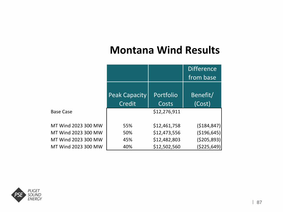
Difference
from base
Peak Capacity
Credit
Portfolio
Costs
Benefit/
(Cost)Base Case $12,276,911
MT Wind 2023 300 MW 55% $12,461,758 ($184,847)
MT Wind 2023 300 MW 50% $12,473,556 ($196,645)
MT Wind 2023 300 MW 45% $12,482,803 ($205,893)
MT Wind 2023 300 MW 40% $12,502,560 ($225,649)
Montana Wind Results

88
Portfolio Sensitivity I – Thermal Mix
June 18, 2015 IRPAG
Annual
Builds (MW) CCCT
Frame
Peaker All Others CCCT
Frame
Peaker All Others CCCT
Frame
Peaker All Others
2016 - - 93 - - 95 - - 93
2017 - - 76 - - 79 - - 76
2018 - - 108 - - 112 - - 108
2019 - - 78 - - 82 - - 78
2020 - - 122 - - 127 - - 122
2021 - - 64 - - 70 - - 64
2022 - - 78 - - 84 - - 78
2023 - 228 159 - - 263 - 228 159
2024 - - 158 385 - 62 - - 158
2025 - - 55 - - 60 - - 55
2026 - 455 29 385 - 30 385 - 29
2027 - - 129 - - 32 385 - 129
2028 - 228 30 - - 132 - - 30
2029 - - 25 - - 27 - - 25
2030 - - 26 385 - 27 - - 26
2031 - 228 29 - - 31 - - 29
2032 - - 35 - - 37 - - 35
2033 - - 46 - - 48 - 228 46
2034 - - 27 - - 28 - - 27
2035 - - 106 - - 27 - - 26
Total - 1,138 1,473 1,156 - 1,454 771 455 1,393
Total
Nameplate
Portfolio NPV
($000)
2,611 2,611
Mix CCCT & Peaker
2,619
12,363,387
Base
12,276,911
All CCCT
12,470,600

89
Total Expected Cost of Portfolios
(Difference from Base Scenario $000)
(6,000,000) (4,000,000) (2,000,000) 0 2,000,000 4,000,000 6,000,000
Recip Engine updated cost
Gas Plant Location
Thermal Mix
Energy Storage in 2023
Gas Transport for Peakers
Carbon Reduction
No DSR
Gas Price
CO2 Price
Demand
Scenario
Total Portfolio Cost (Difference from Base $000)
Low
High
Very High
Base = 0Low High
Base + Low Demand
Base + High Demand
Base + No CO2
Base + High CO2
Base + Low Gas Price
Base + Very High Gas Price
Base + High Gas Price
75 MW in 2035
75 MW in 2023
80 MW Battery
80 MW Pumped Hydro
300 MW Wind in 2021
300 MW Solar in 2021
Mix CCCT & Frame
All CCCT
224 MW in 2035
Factors out of
our control
Decisions we
can control

Electric Stochastic
Modeling Villamor Gamponia & Elizabeth Hossner
June 18, 2015 IRPAG

91
Model Overview – Electric Analysis
June 18, 2015 IRPAG
AuroraXMP
Develops scenario prices and dispatched resource outputs, costs and revenues for each input draw
Stochastic Model
Develops distribution of inputs:Electric and Gas Prices
PSE LoadsHydro and Wind Generation
CO2 Cost/PriceThermal Forced Outage Rates
PSM III
Uses PSE financial model to develop optimal portfolio for each
scenario

92
Stochastic Model: Goal
June 18, 2015 IRPAG
• Challenge is to capture risk in a systematic and consistent
way
• Key correlations across risk variables and time
• Identify major sources of risks
• Weather (Temperature, Hydro Conditions, Wind)
• Market (Economic/Population/Gas & Power)
• Regulation – CO2
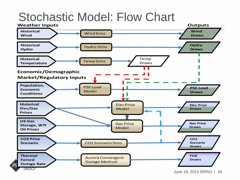
93
Stochastic Model: Flow Chart
June 18, 2015 IRPAG
Weather Inputs Outputs
Economic/Demographic
Market/Regulatory Inputs
Historical Wind
Historical Hydro
Historical Temperature
Historical Elec/Gas Prices
Population,Economic Conditions
US Gas Storage, WTI Oil Prices
Wind Sims
Hydro Sims
Temp Sims
Wind Draws
Hydro Draws
Temp Draws
PSE LoadModel
Elec Price Model
Gas Price Model
PSE Load Draws
Elec Price Draws
Gas Price Draws
CO2 PriceScenario CO2 Scenario Sims
CO2 ScenarioDraws
Thermal Forced Outage Rate
Aurora Convergent Outage Method
FOR Draws

94
Stochastic Inputs for Portfolio Modeling
June 18, 2015 IRPAG
• 250 Draws for each of the inputs
• Mid-C Power Prices
• Sumas Gas Prices
• CO2 Prices
• Wind Generation
• Hydro Generation
• PSE Demand – Peak and Energy
• Thermal Plant Forced Outage

95
Stochastic Inputs: Power & Gas Price Equations
June 18, 2015 IRPAG
Econometric equations in semi-log form
MidC Price = f(Sumas Price, Regional Temp Devs, Day of Week, Holidays,
MidC Hydro Generation)
Sumas Price = f(US Gas Storage Devs fr 5Yr Avg, WTI, lagged WTI, Trend,
Fracking)
AECO Price = f(Sumas Price)
Data – daily data from 1/2003 to 12/2014
Equations were estimated simultaneously with autocorrelation(to
be shown in the Appendix)
WTI = West Texas Intermediate Oil Price
96
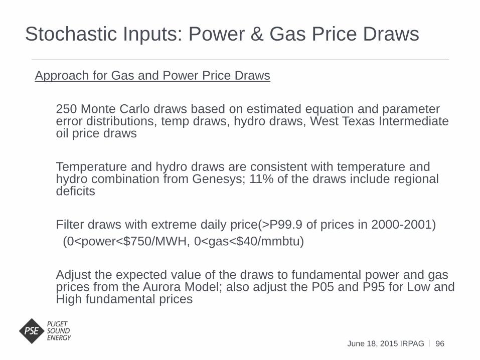
Stochastic Inputs: Power & Gas Price Draws
June 18, 2015 IRPAG
Approach for Gas and Power Price Draws
250 Monte Carlo draws based on estimated equation and parameter error distributions, temp draws, hydro draws, West Texas Intermediate oil price draws
Temperature and hydro draws are consistent with temperature and hydro combination from Genesys; 11% of the draws include regional deficits
Filter draws with extreme daily price(>P99.9 of prices in 2000-2001)
• (0<power<$750/MWH, 0<gas<$40/mmbtu)
Adjust the expected value of the draws to fundamental power and gas prices from the Aurora Model; also adjust the P05 and P95 for Low and High fundamental prices
97
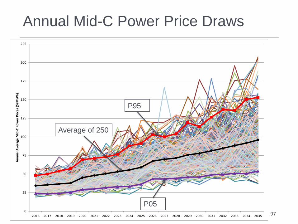
Annual Mid-C Power Price Draws
June 18, 2015 IRPAG 0
25
50
75
100
125
150
175
200
225
2016 2017 2018 2019 2020 2021 2022 2023 2024 2025 2026 2027 2028 2029 2030 2031 2032 2033 2034 2035
An
nu
al A
vera
ge M
id-C
Po
wer
Pri
ces
($/M
Wh
)
Average of 250
P95
P05

98
Annual Sumas Gas Price Draws
June 18, 2015 IRPAG 0
2
4
6
8
10
12
14
16
2016 2017 2018 2019 2020 2021 2022 2023 2024 2025 2026 2027 2028 2029 2030 2031 2032 2033 2034 2035
Ann
ual A
vera
ge S
umas
Gas
Pri
ce ($
/MM
Btu
)
P95
P05

99
MidC Price Distribution for Operating Year
2020-2021
June 18, 2015 IRPAG
10
0
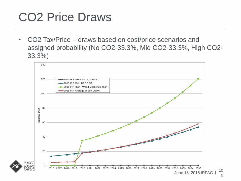
CO2 Price Draws
June 18, 2015 IRPAG
• CO2 Tax/Price – draws based on cost/price scenarios and
assigned probability (No CO2-33.3%, Mid CO2-33.3%, High CO2-
33.3%)
0
20
40
60
80
100
120
140
2016 2017 2018 2019 2020 2021 2022 2023 2024 2025 2026 2027 2028 2029 2030 2031 2032 2033 2034 2035
No
min
al
$/t
on
2015 IRP Low - No CO2 Price
2015 IRP Mid - NPCC CA
2015 IRP High - Wood Mackenzie High
2015 IRP Average of 250 Draws
10
1
Wind Generation
June 18, 2015 IRPAG
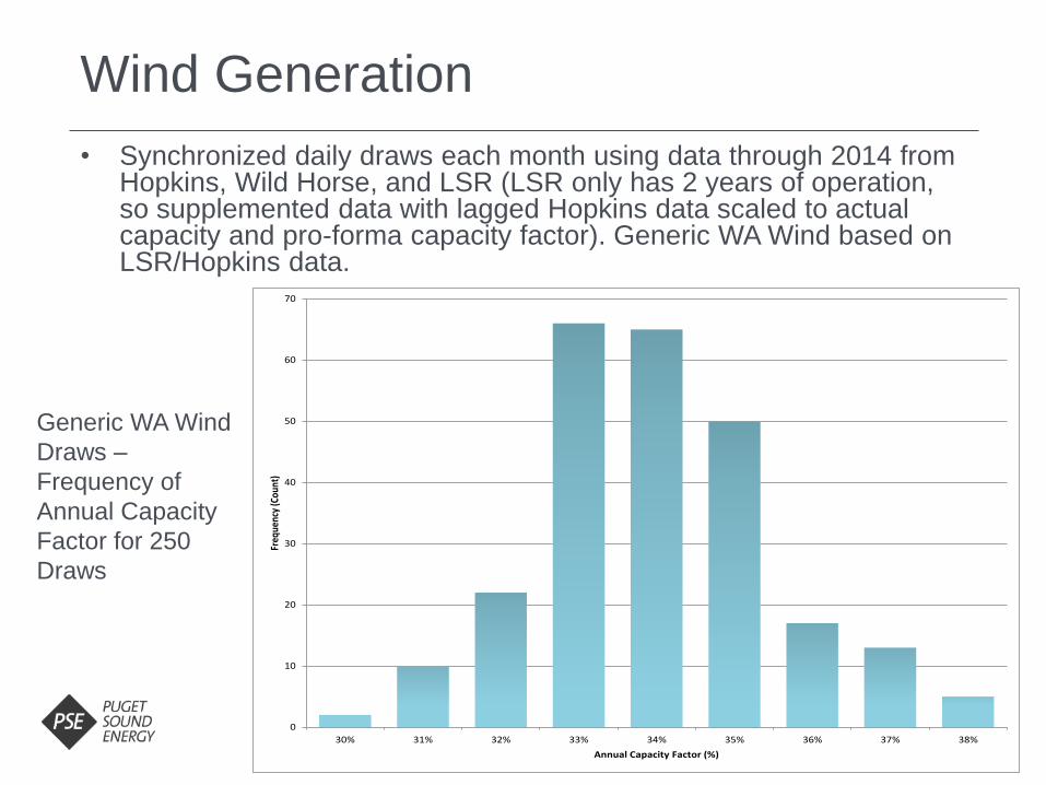
• Synchronized daily draws each month using data through 2014 from Hopkins, Wild Horse, and LSR (LSR only has 2 years of operation, so supplemented data with lagged Hopkins data scaled to actual capacity and pro-forma capacity factor). Generic WA Wind based on LSR/Hopkins data.
0
10
20
30
40
50
60
70
30% 31% 32% 33% 34% 35% 36% 37% 38%
Freq
uenc
y (C
ount
)
Annual Capacity Factor (%)
Generic WA Wind
Draws –
Frequency of
Annual Capacity
Factor for 250
Draws

10
2
Generic WA Wind Draws –
Monthly Capacity Factor for 250 Draws
June 18, 2015 IRPAG
0%
10%
20%
30%
40%
50%
60%
70%
1 2 3 4 5 6 7 8 9 10 11 12
Mon
thly
Cap
acit
y Fa
ctor
(%)
Month
Average of 250
10
3
Hydro Generation
June 18, 2015 IRPAG
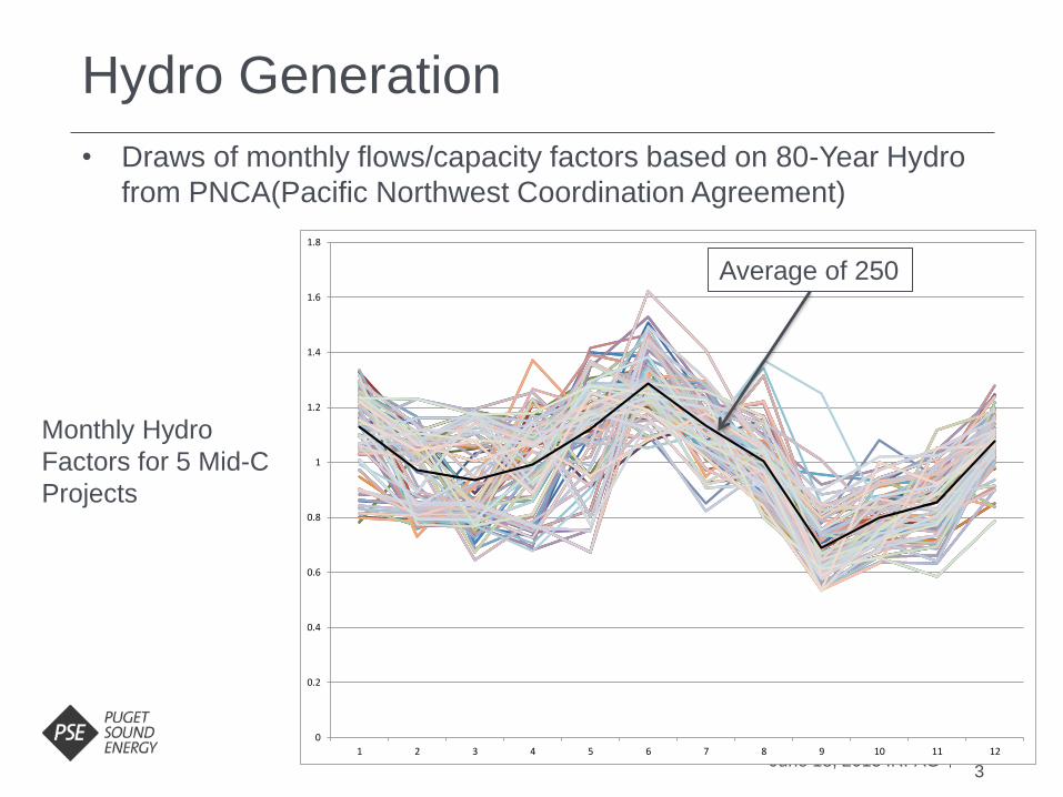
• Draws of monthly flows/capacity factors based on 80-Year Hydro
from PNCA(Pacific Northwest Coordination Agreement)
0
0.2
0.4
0.6
0.8
1
1.2
1.4
1.6
1.8
1 2 3 4 5 6 7 8 9 10 11 12
Average of 250
Monthly Hydro
Factors for 5 Mid-C
Projects

10
4
Demand Draws
June 18, 2015 IRPAG
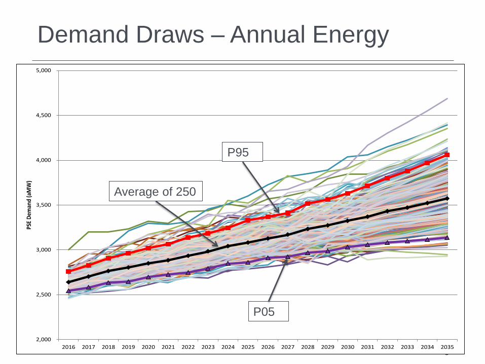
• Monte Carlo draws on economic and demographic inputs are
based on historical standard errors of growth in macroeconomic
and key regional inputs into the model such as population,
employment and income;
• The stochastic simulation also accounts for the error distribution
of the estimated customer counts and use per customer
equations and the estimated equation parameters;
• Temperature draws used on 1929-1947 Portage Bay data (near
UW) and 1948-2005 SeaTac data; HDDs/CDDs based on each
temperature year draw is run through the demand forecast model;
impacts on monthly/hourly profile and use/customer
10
5
Demand Draws – Annual Energy
June 18, 2015 IRPAG 2,000
2,500
3,000
3,500
4,000
4,500
5,000
2016 2017 2018 2019 2020 2021 2022 2023 2024 2025 2026 2027 2028 2029 2030 2031 2032 2033 2034 2035
PSE
Dem
and
(aM
W)
Average of 250
P95
P05

10
6
Demand Draws - Peak
June 18, 2015 IRPAG 4,000
4,500
5,000
5,500
6,000
6,500
7,000
7,500
8,000
8,500
9,000
2016 2017 2018 2019 2020 2021 2022 2023 2024 2025 2026 2027 2028 2029 2030 2031 2032 2033 2034 2035
PSE
Peak
Dem
and
(MW
)
Average of 250
P95
P05

10
7
Stochastic Results
10
8
Stochastic Analysis Results
June 18, 2015 IRPAG
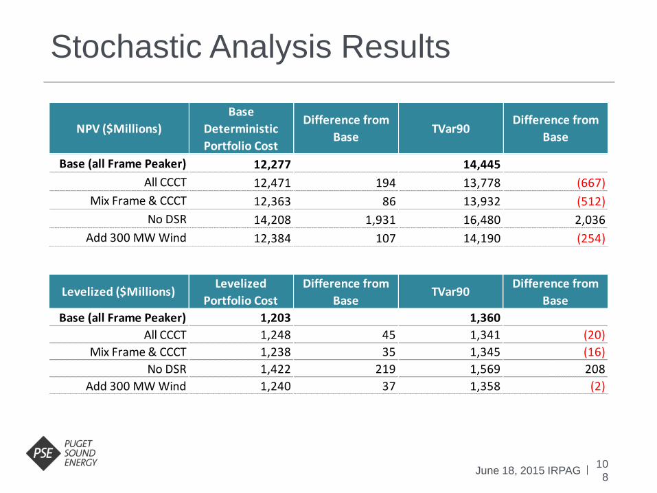
NPV ($Millions)
Base
Deterministic
Portfolio Cost
Difference from
BaseTVar90
Difference from
Base
Base (all Frame Peaker) 12,277 14,445
All CCCT 12,471 194 13,778 (667)
Mix Frame & CCCT 12,363 86 13,932 (512)
No DSR 14,208 1,931 16,480 2,036
Add 300 MW Wind 12,384 107 14,190 (254)
Levelized ($Millions)Levelized
Portfolio Cost
Difference from
BaseTVar90
Difference from
Base
Base (all Frame Peaker) 1,203 1,360
All CCCT 1,248 45 1,341 (20)
Mix Frame & CCCT 1,238 35 1,345 (16)
No DSR 1,422 219 1,569 208
Add 300 MW Wind 1,240 37 1,358 (2)

10
9
Stochastic Results
June 18, 2015 IRPAG
14,444,667
13,777,824 13,932,247
16,480,448
14,190,391
0
2,000,000
4,000,000
6,000,000
8,000,000
10,000,000
12,000,000
14,000,000
16,000,000
18,000,000
20,000,000
Base_All FramePeaker
All CCCT Mix CCCT & Frame No DSR Add 300 MW Wind
Expe
cted
Por
tfol
io C
ost (
$000
)
Expected Portfolio Cost
Q1 (P25)
Min
Median (P50)
Max
Q3 (P75)
Base Deterministic
TVar90

11
0
0
20
40
60
80
100
120
140
Fre
qu
en
cy (
Co
un
t)Frequency Histogram of Expected Portfolio Cost (Billions $)
Base Portfolio
Base_No DSR
Base Portfolio mean = $11.1
Base_No DSR mean = $12.9
11
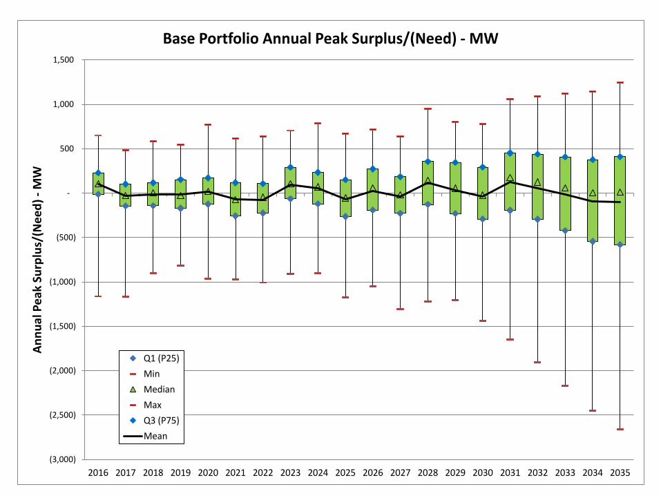
1
(3,000)
(2,500)
(2,000)
(1,500)
(1,000)
(500)
-
500
1,000
1,500
2016 2017 2018 2019 2020 2021 2022 2023 2024 2025 2026 2027 2028 2029 2030 2031 2032 2033 2034 2035
An
nu
al P
ea
k Su
rplu
s/(N
ee
d)
-M
WBase Portfolio Annual Peak Surplus/(Need) - MW
Q1 (P25)
Min
Median
Max
Q3 (P75)
Mean
11
2
Net Cost of Capacity

11
3
Cost of Incremental Capacity
June 18, 2015 IRPAG
Based on PSM for the 2015 IRP
NPV to 2016($000s)
Net Cost w/o
Replacement
Replacement
Cost
Net Cost w
Replacement
Levelized
Cost
Capacity
(MW)
Levelized
Cost/MW
New CCCT 2020 738,139 82,828 820,967 61,862 385 160.68
New Peaker Aero 2020 424,201 41,696 465,897 35,551 203 175.13
New Peaker Frame 2020 385,692 44,890 430,582 32,324 228 141.77
New Peaker Recip 2020 569,848 47,893 617,741 47,758 220 217.08
2. Base - 2015 IRP
NPV to 2016 ($000)
Net Cost w/o
Replacement
Replacement
Cost
Net Cost w
Replacement
Levelized
Cost
Capacity
(MW)
Levelized
Cost/MW
New CCCT 2020 640,446 64,147 704,593 53,674 385 139.41
New Peaker Aero 2020 418,176 40,263 458,439 35,046 203 172.64
New Peaker Frame 2020 390,542 47,680 438,222 32,730 228 143.55
New Peaker Recip 2020 567,329 48,743 616,072 47,546 220 216.12
7. Base + No CO2 - 2015 IRP
11
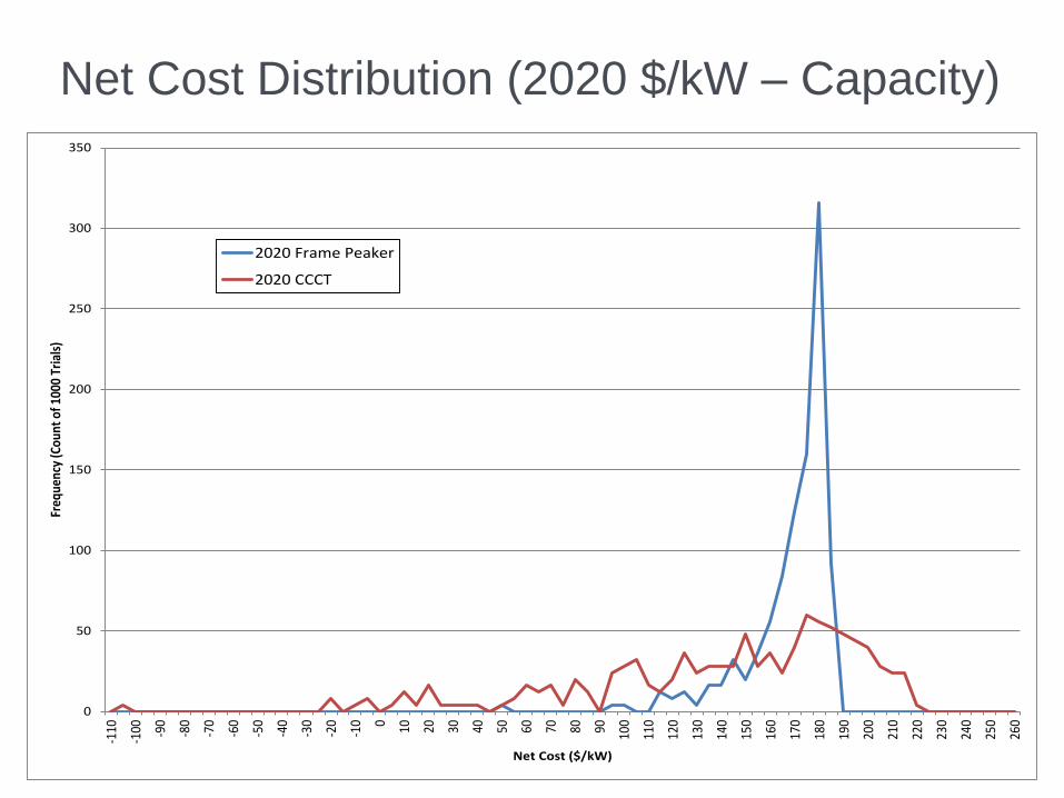
4
Net Cost Distribution (2020 $/kW – Capacity)
0
50
100
150
200
250
300
350
-110
-100 -9
0
-80
-70
-60
-50
-40
-30
-20
-10 0 10 20 30 40 50 60 70 80 90 100
110
120
130
140
150
160
170
180
190
200
210
220
230
240
250
260
Freq
uenc
y (C
ount
of 1
000
Tria
ls)
Net Cost ($/kW)
2020 Frame Peaker
2020 CCCT

Wrap Up/Review Action
Items Lyn Wiltse
June 18, 2015 IRPAG

11
6 June 18, 2015 IRPAG
Adjourn


