Is fiscal devaluation welfare enhancing?

A model-based analysis

Stefan Hohbergera Lena Krausa

a University of Bayreuth

Abstract:

Large trade imbalances have emerged as major policy challenges for the euro area within the

last decade. As fiscal policy is the major macroeconomic policy instrument left with the

individual member countries of EMU, fiscal devaluation is a highly debated policy tool to

mimic the effects of an external devaluation by implementing a budgetary-neutral tax shift

from direct to indirect taxes. This paper uses a two-region tow-sector DSGE model with

nominal wage and price rigidities to analyse the welfare effects of fiscal devaluation

understood as tax shift from social security contributions for employers to value-added tax in

a small open economy in monetary union. This paper finds that fiscal devaluation can stabilise

excessive trade balance fluctuations, but implies welfare losses for the average household.

The results are robust to several sensitivity checks, in particular to alternative fiscal budget

closures and changes in the relative sector composition.

JEL classification: E62, F32, F41 Keywords: fiscal devaluation, external imbalances, monetary union, welfare Corresponding author: Author: Lena Kraus Stefan Hohberger (lena-maria.kraus@uni-bayreuth.de) (stefan.hohberger@uni-bayreuth.de) University of Bayreuth University of Bayreuth Germany Germany

1

1. Introduction

Since the establishment of the European Monetary Union (EMU) in 1999, the issue of

growing and persistent external imbalances among several EMU countries has attracted a lot

of interest. Due to the elimination of exchange rate risk and the disappearance of country risk

premia, capital flows in the periphery countries and led to a demand boom with concomitant

increases in domestic prices and labour costs. The subsequent competitiveness losses resulted

in growing trade balance deficits. In consequence of the loss of both autonomous monetary

policy and the possibility of nominal exchange rate (external) devaluation, it is of particular

interest to analyse alternative stabilisation tools in order to regain competitiveness. As fiscal

policy is the major macroeconomic policy instrument left with the individual member

countries of EMU, this poses new challenges for the appropriate design of tax and expenditure

policies.

An alternative to nominal exchange rate devaluation might be a fiscal devaluation, which

mimics the effects of an external devaluation by implementing a budgetary-neutral tax shift

from direct to indirect taxes. In particular, taxes are shifted from social security contributions

(SSC) for employers to value-added tax (VAT) in order to make exports cheaper and imports

more expensive. The effect of such an internal devaluation is based on the assumption of rigid

wages: if a reduction in employers’ SSC rate is not immediately accompanied by higher

nominal wages, firms face lower labour costs, leading to lower prices and higher exports (de

Mooij and Keen, 2012). In the long run, however, labour unions could push through higher

wages in order to compensate for higher consumption expenditures.

The existing literature on fiscal devaluation focuses on the reduction of excessive and

persistent trade balance deficits within the EMU by analysing a revenue-neutral tax shift,

implemented as an exogenous shock (e.g. Engler et al. 2014; Lipinska and von Thadden 2012;

Langot et al. 2012; Stähler and Thomas 2012). While Lipinska and von Thadden (2012)

examine a tax shift from labour income tax to VAT, Engler et al. (2014) use a two-region

framework (northern and southern European countries) and analyse a reduction in employers’

SSC accompanied by a rise in VAT as a quasi-permanent tax shift. They find that a fiscal

devaluation in southern European countries increases output by around 1 percent and

improves the trade balance by 0.2 percent of GDP. Stähler and Thomas (2012) use a two-

country monetary union model to simulate a number of policy measures aimed at achieving a

2

fiscal devaluation in Spain. They find that a shift of employers’ SSC to VAT in the sense that

the primary deficit-to-GDP ratio decreases by one percentage point ex ante can improve

Spain’s competitiveness significantly in the long run. Hohberger et al. (2014) focus their

analysis rather on budgetary-neutral government expenditure shifts between tradable and non-

tradable goods, but use fiscal devaluation, i.e. a tax shift between labour and consumption tax,

as benchmark scenario. Langot et al. (2012) provide an optimal tax scheme for a fiscal

devaluation that is welfare enhancing for households. Commonly, however, the existing

literature on fiscal devaluation focuses primarily on regaining international competitiveness

and neglect associated welfare effects.

This paper builds on the recent literature on fiscal devaluation (e.g., Lipinska and von

Thadden 2012; Langot et al. 2012; Stähler and Thomas 2012; Engler et al. 2014; Hohberger et

al. 2014) and analyses a revenue-neutral tax-shift from employers SSC to consumption tax

(VAT) in order to reduce excessive external fluctuations caused by supply and demand

shocks. Additionally, this paper broadens the analysis in several dimensions by (i) considering

fiscal devaluation as an instrument rule that adjusts taxes in response to external fluctuations,

(ii) examining the welfare effects of fiscal devaluation in the context of a standard assessment

of household welfare and (iii) providing sensitivity results, e.g. for alternative fiscal budget

closures.

The analytical framework is a two-sector New Keynesian DSGE model of monetary union

according to Hohberger et al. (2014) and follows the small open economy approach by Galí

and Monacelli (2008). The focus on a small member country of monetary union approach

excludes feedback from domestic events to monetary policy and the rest of monetary union

and is of particular interest for analysing stabilisation tools since small countries tend to be

more exposed to asymmetric shocks.

The paper finds that fiscal devaluation understood as tax shift from employers’ SSC to VAT

can stabilise excessive fluctuations in the trade balance, but induces welfare losses for the

average household. More precisely, LC households that do not have access to financial

markets experience higher welfare losses than those households (Ricardian) that are able to

smooth consumption over time.

3

2. Model

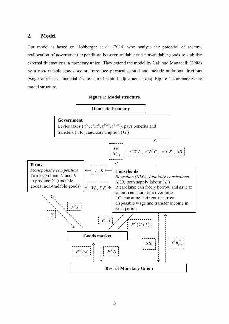
Our model is based on Hohberger et al. (2014) who analyse the potential of sectoral

reallocation of government expenditure between tradable and non-tradable goods to stabilise

external fluctuations in monetary union. They extend the model by Galí and Monacelli (2008)

by a non-tradable goods sector, introduce physical capital and include additional frictions

(wage stickiness, financial frictions, and capital adjustment costs). Figure 1 summarises the

model structure.

Figure 1: Model structure.

Domestic Economy

Government Levies taxes ( w c k SCee SCer, , , , ), pays benefits and transfers ( TR ), and consumption ( G )

Firms Monopolistic competition Firms combine L and K to produce Y (tradable goods, non-tradable goods)

Households Ricardian (NLC), Liquidity-constrained (LC); both supply labour ( L ) Ricardians: can freely borrow and save to smooth consumption over time LC: consume their entire current disposable wage and transfer income in each period

Goods market

Rest of Monetary Union

, , , w c C k ktW L P C i K B

TR

1tiB

, L K

, kWL i K

YP Y

YC I

CP C I

FtB 1

F Fti B

XP XMP IM

4

We augment this model by adding social contribution costs for employers and employees as

wells as lump-sum and capital taxes as alternative budget closures. The model includes

monopolistic competition in goods and labour markets, nominal price and wage stickiness,

liquidity constraints, capital and labour as production factors and a set of tax variables in

order to analyse the impact of fiscal devaluation on domestic activity and household welfare.

Households are either intertemporal optimising consumers (NLC) that can freely borrow and

save to smooth consumption over time, or liquidity-constrained (LC) households without

access to financial markets who consume their entire current disposable wage in each period.

We depart from the assumption of complete risk-sharing as in Galí and Monacelli (2008) and

introduce a debt-dependent country risk premium (Schmitt-Grohé and Uribe 2003) as external

closure. Goods markets are imperfectly integrated across borders in the sense that there is

home bias in the demand for goods. Labour is immobile between countries. The RoEA

variables and monetary policy are exogenously given from the perspective of the small

economy. A detailed description of the model can be found in Hohberger et al. (2014).

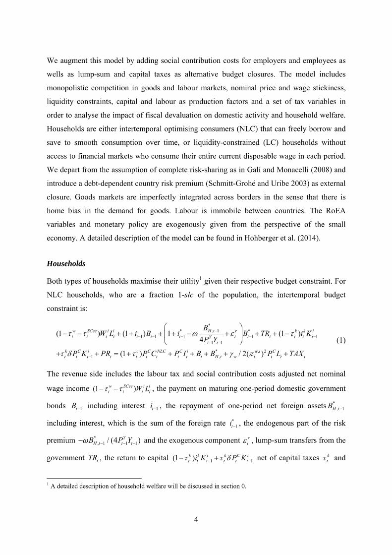
Households

Both types of households maximise their utility1 given their respective budget constraint. For

NLC households, who are a fraction 1-slc of the population, the intertemporal budget

constraint is:

*, 1* *

1 1 1 1 11 1

* , 21 ,

(1 ) (1 ) 1 (1 )4

(1 ) / 2( )

H tw SCee i i r k k it t t t t t t t t t t t tY

t t

k C i c C NLC C i w i Ct t t t t t t t t t H t w t t t t

BW L i B i B TR i K

P Y

P K PR P C P I B B P L TAX

(1)

The revenue side includes the labour tax and social contribution costs adjusted net nominal

wage income (1 ) w SCee i it t t tW L , the payment on maturing one-period domestic government

bonds 1tB including interest 1ti , the repayment of one-period net foreign assets *, 1H tB

including interest, which is the sum of the foreign rate *1ti , the endogenous part of the risk

premium *, 1 1 1/ (4 ) Y

H t t tB P Y and the exogenous component rt , lump-sum transfers from the

government tTR , the return to capital 1 1(1 ) k k i k C it t t t t ti K P K net of capital taxes k

t and

1 A detailed description of household welfare will be discussed in section 0.

5

depreciation allowances kt , where , , i i i

t T t NT tK K K , and profit income tPR from firm

ownership. The expenditure side combines nominal consumption C NLCt tP C taxed at rate c

t ,

where CtP is the consumer price index (CPI), nominal investment in the tradable and non-

tradable sector C it tP I , where , , i i i

t T t NT tI I I , financial investment in domestic bonds and (net)

foreign assets, and quadratic costs w of wage adjustment ( ,1/ 1w i i i

t t tW W ). The

introduction of lump-sum tax tTAX as non-distortionary tax becomes is crucial when

discussing alternative budget closures.

The period budget constraint of LC households constituting the share slc of the population is:

, 2(1 ) (1 ) / 2( ) t

w SCee i i LC c C LC w i C LCt t t t t t t t w t tW L TR P C P L (2)

The per-capita level of consumption in the aggregate is the weighted average of NLC and LC

consumption:

(1 ) NLC LCt t tC slc C slcC (3)

Private demand combines domestically produced tradable ( ,iTH tC , ,

iTH tI ), non-tradable

( ,iNT tC , ,

iNT tI ) and imported ( ,

iTF tC , ,

iTF tI ) goods. Assuming the same trade price elasticity for

consumption and investment demand, we can aggregate ( , , )NLC LCt t t tZ C C I and define tZ as

a CES aggregate of tradable ( ,iT tZ ) and non-tradable goods ( ,

iNT tZ ):

1 1 1 1 1

, ,( ) ( ) (1 ) ( )

t T t NT tZ Z Z

(4)

where and is the share of tradable goods and the elasticity of substitution between

tradable and non-tradable goods, respectively. ,T tZ is a composite index of domestically

produced tradable goods ( ,TH tZ ) and imported goods ( ,TF tZ ) defined by:

1 1 1 1 1

, , ,( ) ( ) (1 ) ( )

T t TH t TF tZ h Z h Z

(5)

6

where h represents the steady state home bias and indicates the elasticity of substitution

between domestically produced goods and imports.

The domestic consumer price index ( CtP ) is given by:

11 1 1

, ,( )( ) (1 )( ) C

t T t NT tP P P (6)

where the domestic country price index for tradable goods ( ,T tP ) has the following form:

11 1 1

, , ,( )( ) (1 )( ) T t TH t TF tP h P h P (7)

Franco (2011) states that the effects of fiscal devaluation on the trade balance is mitigated by

an increase in the non-tradable sector, as the price of tradables and non-tradables of domestic

produced goods decreases through the tax shift away from employers’ social security

contributions, while prices of foreign produced goods do not change. Therefore, tradable

goods as a composite of foreign and domestic produced tradable goods are relative expensive

compared to non-tradable goods after fiscal devaluation has taken place. In section 5, we

examine the role of the relative size between the two sectors and the subsequent welfare

effects in a sensitivity analysis.

The households supply labour services to both tradable and non-tradable goods sectors. The

labour services are distributed equally across NLC and LC households, and specialised labour

unions represent the different types of labour services i in the wage setting. The wage setting

is subject to quadratic adjustment costs, which provide an incentive to smooth the wage

adjustment and lead to nominal wage stickiness. Since we assume identical wages itW for

both sectors, the optimisation problem of the labour union representing the labour service i is:

,1 , 20 0

( ) (1 ) ( )1 2

i

TH tt i i w SCee i i w it wt t t t t t t tC Ct

t t

PWE L L L

P P (8)

The optimisation problem is symmetric across unions i, which implies identical wages

( it tW W ) and labour demand ( i

t tL L ) across households. Hence, the aggregate wage setting

equation is:

7

, , 11 1 11

1 1

(1 )

1 1 1

w SCee tt t C

t

totTH t TH tw wt w t w t t t

t t ttot C tot Ct t t t t t t

W

P

P PL W W LE

W P W P L

(9)

where the gross wage claims increase with increasing labour taxation ( wt ) and social

contribution costs ( SCeet ) for given levels of employment.

Firms

The economy consists of a continuum of monopolistically competitive firms in the tradable

and non-tradable sector, are owned by NLC households and produce a differentiated good ,j

s tY

with capital , 1j

s tK , labour ,js tL and Cobb-Douglas production technology in each sector s :

1, , , 1 ,( ) ( )j j j

s t s t s t s tY A K L (10)

The cost-minimal combination of capital and labour is given by:

,

, 1

1

(1 )

j ks t tj SCer

s t t t

L i

K W

(11)

which implies for the nominal marginal costs ,j

s tMC of the optimising firm:

1

, 1,

( ) [(1 ) ]

(1 )

k SCerj t t t

s ts t

i WMC

A

(12)

The employers’ SSC is given by SCert . The higher the employers’ SSC is as percentage of

gross wage earnings, the lower is the use of labour in the production of good ,j

s tY .

The firms in each sector s face quadratic price adjustment costs p and set prices ,j

s tP to

maximise the discounted expected profit. For each sector, firms profit maximization has the

following form:

, , , 20 , , . ,0

0 , ,

(1 )( )

2

j SCer jNLCps t t s tt j j p jt

s t s t s t s tNLCts t s t

P WE Y L Y

P P (13)

The nominal GDP is the sum of domestically produced tradable and non-tradable output:

8

, , , , Yt t TH t T t NT t NT tP Y P Y P Y (14)

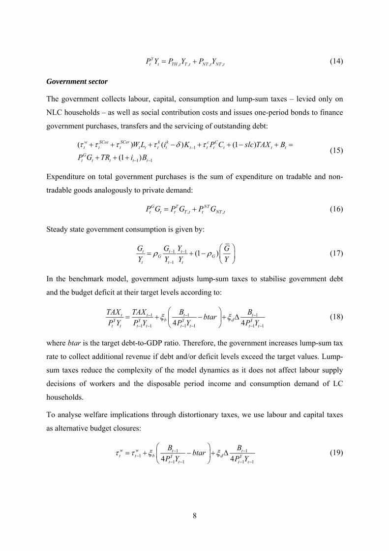
Government sector

The government collects labour, capital, consumption and lump-sum taxes – levied only on

NLC households – as well as social contribution costs and issues one-period bonds to finance

government purchases, transfers and the servicing of outstanding debt:

1

1 1

( ) ( ) (1 )

(1 )

w SCee SCer k k c Ct t t t t t t t t t t t t

Gt t t t t

W L i K P C slc TAX B

P G TR i B (15)

Expenditure on total government purchases is the sum of expenditure on tradable and non-

tradable goods analogously to private demand:

, ,G T NT

t t t T t t NT tP G P G P G (16)

Steady state government consumption is given by:

1 1

1

(1 )

t t t

G Gt t t

G G Y G

Y Y Y Y (17)

In the benchmark model, government adjusts lump-sum taxes to stabilise government debt

and the budget deficit at their target levels according to:

1 1 1

1 1 1 1 1 14 4

t t t t

b dY Y Y Yt t t t t t t t

TAX TAX B Bbtar

P Y P Y P Y P Y (18)

where btar is the target debt-to-GDP ratio. Therefore, the government increases lump-sum tax

rate to collect additional revenue if debt and/or deficit levels exceed the target values. Lump-

sum taxes reduce the complexity of the model dynamics as it does not affect labour supply

decisions of workers and the disposable period income and consumption demand of LC

households.

To analyse welfare implications through distortionary taxes, we use labour and capital taxes

as alternative budget closures:

1 11

1 1 1 14 4w w t tt t b dY Y

t t t t

B Bbtar

P Y P Y

(19)

9

1 11

1 1 1 14 4k k t tt t b dY Y

t t t t

B Bbtar

P Y P Y

(20)

Fiscal devaluation is simulated as a revenue-neutral tax shift between employers’ SSC and

consumption tax in response to fluctuations in the trade balance gap /TB Y or trade balance

level /TB Y :

1 (1 ) (1 )c c ct G t G G Z tZ (21)

with [ / , / ]tZ TB Y TB Y and:

1 (1 ) ( )C

SCer SCer SCer c c t tt G t G t t

t t

P C

W L

(22)

The tax shift is revenue-neutral in the sense that the overall level of government revenues is

kept constant. A negative parameter value ( Z 0 ) implies an increase in consumption tax

and a decline in employers’ SSC in case of an excessive trade balance deficit in order to

mimic the real effects of nominal exchange rate depreciation.

External Account

The total demand for domestic output is the sum of final domestic demand, net exports and

the wage/price adjustment costs tADC :

,( ) Y C G THt t t t t t t t t TF t t tP Y P C I P G P X P M ADC (23)

Exports tX correspond to the import demand of the rest of monetary union (RoMU):

* *, ,(1 )( / ) t TH t TH t tX h P P Y (24)

which uses the fact that the tradable prices in the RoMU and the prices of tradables produced

in RoMU are (almost) identical from the perspective of the small domestic economy. We

exclude price discrimination between countries, i.e. the law of one price holds.

The aggregate resource constraint of the domestic economy, which is also the law of motion

for the net foreign asset (NFA) position, is given by:

* *, 1 , 1(1 ) ( ) Y C G Y

H t t H t t t t t t t t t tB i B P Y P C I P G P ADC (25)

10

The current account equals the change in net foreign assets:

* *, , 1 t H t H tCA B B (26)

We treat RoMU as a single, large country, which engages in trade with the small country.

However, the trade volume with the small country is low, such that RoMU is seen as a closed

economy.

Parameterisation

As the model is supposed to reflect an average small economy in a monetary union, data

information for the exogenous variables and parameters in the model are obtained from the

Eurostat database of the European Commission, the OECD database and further sources in the

literature of DSGE models. The numerical values of the model parameter and steady state

ratios are summarised in Table 1.

The parameter h = 0.51, which is modelled as the home bias for the consumption of goods, is

calculated by deducting the average import-to-GDP ratio of eight small euro area countries

from one for the period 1999-2012.2 The value suggested in the literature for the elasticity of

substitution between tradable and non-tradable goods ranges from a low elasticity, such as

0.13 found by Rabanal and Tuesta (2013) when investigating the role of the non-tradable

sector for the dynamics of the real exchange rate, to a high elasticity of 0.74 for industrial

countries estimated by Mendoza (1995). This paper adheres to = 0.5, which is used by

Gomes et al. (2010), who establish a model for policy analyses within the euro area.

The euro area average 1999-2012 of government debt/deficit is 74 percent of GDP. Once debt

relative to GDP exceeds its target level of 74 percent, the budget closure rule for debt-to-GDP

stabilisation applies by raising taxes or lowering general transfers. A one percentage point

increase in government debt-to-GDP and the deficit-to-GDP ratio implies a tax increase or

transfer decline of 0.001 percentage points in the case of debt stabilisation and one percentage

point in the case of deficit stabilisation.

2 The respective group of countries comprises Austria, Belgium, Finland, Greece, Ireland, the Netherlands, Portugal and Spain, following Vogel et al. (2013) and Hohberger et al. (2014).

11

Table 1: Parameter and steady state ratios of the model

Structural Parameters Value

Households and Firms

Discount factor 0.995

Consumption relative to GDP C/Y 0.6

Government spending relative to GDP G/Y 0.2

Investment relative to GDP I/Y 0.2

Tradable goods share of GDP T/Y 0.6

Share of LC households slc 0.4

Weight of labour disutility 1.0

Inverse of elasticity of labour supply 4.0

Share of tradable goods in consumption 0.6

Elasticity of substitution T/NT goods 0.5

Intertemporal elasticity of substitution 2.0

Elasticity of substitution between home and foreign goods 2.0

Elasticity of substitution between goods varieties j 0.6

Elasticity of substitution for labour services i 0.6

Steady state level A 0.47

Cobb-Douglas parameter (capital share) 0.4

Coefficient on output growth 0.05

Degree of home bias h 0.51

Wage adjustment costs 80.0

Price adjustment costs 48.0

Capital adjustment costs 30.0

Fiscal Policy

Debt-to-GDP ratio btar 0.74

Fiscal reaction to debt 0.001

Fiscal reaction to deficit 1.0

Persistence of fiscal instrument 0.5

Consumption tax rate 0.197

Labour income tax rate 0.16

Social security contribution of employers 0.25

Social security contribution of employees 0.13

Capital tax rate 0.3

Lump-sum tax rate relative to GDP TX/Y 0.0

General transfers relative to GDP TR/Y 0.12

Shock Calibration

Persistence of TFP shock 0.92

Standard deviation TFP 0.025

Persistence of risk premium shock 0.85

Standard deviation risk premium 0.015

12

The tax rate on consumption of 19.7 percent is given by the average VAT rate within the euro

area for the period 1999-2012 (Taxation Trends in the European Union 2013, EC). The

average tax rate on capital income is 30 percent (OECD Tax Database). Given the total gross

earnings before tax, households pay labour income tax and SSC as a percentage share of their

gross wage earnings to the general government. The average labour income tax burden for the

given period is 16 percent of total earnings plus 13 percent SSC for the households. Thus, the

net income of households amounts to 71 percent of total gross wage earnings. Firms

contribute on average 25 percent social security as a percentage of total gross wage earnings

to the general government. Consequently, the total labour costs of firms reach 125 percent of

gross wage earnings.

The low trade elasticity between domestic and imported tradable goods estimated by Imbs and

Méjean (2010) with η = 1.5 is criticised by Simonovska and Waugh (2014) for not giving

micro-level heterogeneity sufficient consideration. Therefore, the parameter value is increased

to η = 2.0, which is a value in the range of those used in the literature.

While Druant et al. (2009) conduct a firm-level survey for various countries and sectors in the

euro area and find an average adjustment of wages about every 15 months and an average

adjustment of prices about every 10 months, which are used by Engler et al. (2014), the

duration of wage adjustments is two months lower for the group of the eight small euro area

countries. We choose wage and price adjustment costs to match durations of wages and prices

of five and four quarters. The value for capital adjustment costs is taken from Hohberger et al.

(2014).

The integration of LC households explains the simultaneous movement of private

consumption and government spending (Galí et al. 2007). The share of liquidity-constrained

households varies in the literature. Ratto et al. (2009) set rule-of-thumb households at 40

percent of population, Galí and Monacelli (2005) use the factor slc = 0.5 and Marto (2013)

estimates the share of slc = 0.58 for the Portuguese economy. We follow Ratto et al. (2009)

and set slc = 0.4. Alternative values for the share of LC households are tested for the purpose

of robustness in section 5.

13

Table 2 compares moments of the benchmark model under the combination of TFP and risk

premium shocks and the absence of fiscal devaluation to actual data for the group of eigth

smaller European member countries for the period 1999q1-2012q4. It shows that the model

matches important characteristics fairly well. More precisely, the model replicates the

correlation of consumption, employment and the trade balance with output quite well. The

high correlation of government purchases with output is caused by the calibration of

government purchases as a fixed share of GDP in the baseline calibration. Of particular note

is the high volatility of investment, which is in line with the data patterns. The model-

generated volatility of employment is slightly higher compared to actual data. The trade

balance is negatively correlated with output and matches the data pattern, whereas the

volatility of the trade balance is lower than the lowest ranked country in the group of small

euro area countries in actual data. The low volatility of inflation compared to data moments is

related to the assumption of constant import prices.

Table 2: Comparing model and data moments

Variable Baseline calibration Actual data

Correlation with output

Standard deviation

Correlation with output Standard deviation Mean Max Min Mean Max Min

Output 1.00 0.03 1.00 1.00 1.00 0.02 0.04 0.01 Consumption 0.83 0.92 0.85 0,92 0.80 0.88 1.21 0.47 Government 0.93 0.85 0.15 0.61 -0.46 1.28 2.43 0.38 Investment 0.86 1.70 0.82 0.93 0.64 3.64 5.83 1.67 Employment 0.25 1.24 0.64 0.93 0.38 0.76 1.06 0.57 Trade balance -0.21 0.35 -0.27 0.15 -075 1.56 2.25 0.81 Inflation 0.13 0.35 0.46 0.82 -0.28 0.64 0.92 0.43

Note: All moments are based on quarterly data. The variables are in logarithms and hp-filtered with λ=1600 for quarterly data (except trade balance, which is relative to GDP, and inflation, which is the year-on-year percentage change of the Consumer Price Index). The actual data mean is calculated for the group of eight smaller EA-countries for 1999q1-2012q4, namely AUT, BEL, ESP, FIN, GRC, IRL, NLD and PRT. Maximum and minimum values are given by the lowest and highest ranked country for the particular measure. The standard deviation is the standard deviation relative to the standard deviation of output, which is the absolute standard deviation.

14

3. Fiscal devaluation as trade balance stabilisation tool

To analyse the stabilising impact of fiscal devaluation we present simulations for negative

productivity (TFP) and risk premium shocks under different model and policy settings: First,

we show impulse responses (IRFs) for the frictionless (FLEX) economy without price and

wage stickiness and, hence, the optimal reaction of the economy to exogenous shocks.

Second, we display the no-policy case (NP) to illustrate the difference between an economy

with and without price and wage stickiness. Third, we examine the potential of fiscal

devaluation as a tax-shift from employers’ SSC to consumption tax to stabilise the trade

balance. We focus our simulations on the response to both the absolute trade balance as well

as the trade balance gap as target variable. The trade balance gap is defined conventionally as

percentage point (relative to GDP) deviations of actual level from the level that would exist

without price and wage stickiness. Hence, the focus on the trade balance gap allows

examining whether fiscal policy can mitigate excess volatility due to price and wage

adjustment. IRF values are specified in percent, except those for the trade balance,

government debt, and the tax rates, which are given in percentage points.

3.1 Negative economy-wide productivity shock

Figure 2 shows impulse responses (IRFs) for a negative economy-wide TFP shock, simulated

as a temporary 2.5 percentage point decline of the total factor productivity relative to the rest

of monetary union. The flexible economy (FLEX) without wage and price stickiness clearly

mirrors the TFP decline in output by 2.5 percent. Private consumption declines due to an

increase in domestic goods prices, resulting in an appreciation of the real exchange rate and a

trade balance deficit. Price stickiness in the no-policy scenario (NP) delays the increase in

domestic prices and lowers real interest rates, so that consumption and investment declines

more moderately compared to the FLEX economy. The increase in employment by 2.5

percent is associated with the lower productivity level when prices and wages are sticky. The

delayed increase in the real exchange rate deteriorates the trade balance, resulting in a

negative trade balance gap in the medium term.

15

Figure 2: Fiscal devaluation in response to a negative TFP shock

A fiscal devaluation in response to the absolute trade balance deficit (TBY_LEVEL) or the

trade balance gap (TBY_GAP), respectively, implies a tax shift from employers’ SSC rate to

consumption tax. More specifically, a fiscal parameter value of Z 5 in Figure 2 implies a

reduction of employers’ SSC rate of around 1.8 percentage points and an increase in

consumption tax of around 0.7 percentage points for stabilising TBY_LEVEL. As a

consequence, fiscal devaluation reduces the trade balance deficit substantially in the case of

level stabilisation (TBY_LEVEL). For the given parameter value of Z 5 , the reduction of

the trade balance gap (TBY_GAP) is less pronounced because the trade balance gap, i.e. the

difference between the actual and the flexible-economy trade balance, and hence the

associated tax shift is smaller than the trade balance deficit in absolute terms.

By shifting the tax burden from employers to consumers, export prices decline and import

prices increase, as the increase in consumption tax is only levied on imported goods while

exempting exported goods from local firms. The increase in consumption tax of up to 0.7

percentage points and the corresponding reduction of labour costs in the production process

through the decrease in SSC dampens the real exchange rate appreciation and the decline in

net exports. As a result, the trade balance improves compared to the NP case. As the real

exchange rate appreciation under fiscal devaluation is only slightly lower than without policy

-2

-1.5

-1

-0.5

0

0.5

1

0 2 4 6 8 10 12Quarter

Tax shift

TBY_LEVEL_C TBY_GAP_C

TBY_LEVEL_SSC TBY_GAP_SSC

PP

0

0.3

0.6

0.9

1.2

1.5

1.8

0 2 4 6 8 10 12

%

Quarter

Real exchange rate

FLEX NP

TBY_LEVEL TBY_GAP

-0.4

-0.3

-0.2

-0.1

0

0 2 4 6 8 10 12Quarter

Trade balance

FLEX NPTBY_LEVEL TBY_GAP

% of GDP

-3

-2.5

-2

-1.5

-1

-0.5

0

0 2 4 6 8 10 12

%

Quarter

Output

FLEX NP

TBY_LEVEL TBY_GAP

-0.5

0

0.5

1

1.5

2

2.5

3

0 2 4 6 8 10 12

%

Quarter

Employment

FLEX NP

TBY_LEVEL TBY_GAP

-1.8

-1.5

-1.2

-0.9

-0.6

-0.3

0

0 2 4 6 8 10 12

%

Quarter

Consumption

FLEX NP

TBY_LEVEL TBY_GAP

16

intervention, the mitigation of a fall in net exports and the trade balance improvement are

rather small, in particular when concentrating on the trade balance gaps. Furthermore, Figure

2 underlines the necessity that increasing taxes on consumption (in percentage points) are less

than decreasing employers’ SSC in order to ensure that the fiscal reform is budgetary-neutral.

This is in line with Langot et al. (2012), who attribute this unproportional tax shift to a higher

tax base for consumption tax than for employers’ SSC.

The effects of fiscal devaluation on domestic variables, e.g. output, consumption and

employment, are rather small compared to the simulation results without fiscal intervention in

the NP economy. While consumption decreases slightly due to higher consumption taxes,

output and employment volatilities remain fairly unchanged.

3.2 Negative risk premium shock (demand boom)

Figure 3 shows impulse responses for a negative risk premium shock of 1.5 percentage points

relative to the rest of monetary union.

Figure 3: Fiscal devaluation in response to a negative risk premium shock.

Note: Welfare is measured relative to non-stabilisation and expressed in % of steady state consumption.

The negative risk premium shock induces a decline in domestic interest rates. Hence,

individuals face lower borrowing rates, which strengthen domestic consumption and

-5

-4

-3

-2

-1

0

1

2

3

0 2 4 6 8 10 12Quarter

Tax shift

TBY_LEVEL_C TBY_GAP_CTBY_LEVEL_SSC TBY_GAP_SSC

pp

-0.3

0

0.3

0.6

0.9

1.2

1.5

0 2 4 6 8 10 12

%

Quarter

Real exchange rate

FLEX NP

TBY_LEVEL TBY_GAP

-1.2

-0.9

-0.6

-0.3

0

0 2 4 6 8 10 12Quarter

Trade balance

FLEX NP

TBY_LEVEL TBY_GAP

% of GDP

-0.5

0

0.5

1

1.5

2

0 2 4 6 8 10 12

%

Quarter

Output

FLEX NP

TBY_LEVEL TBY_GAP

-0.5

0

0.5

1

1.5

2

2.5

3

0 2 4 6 8 10 12

%

Quarter

Employment

FLEX NP

TBY_LEVEL TBY_GAP

0

0.5

1

1.5

2

2.5

0 2 4 6 8 10 12

%

Quarter

Consumption

FLEX NP

TBY_LEVEL TBY_GAP

17

investment demand and also the demand for imports. The increase in domestic demand puts

upward pressure on price and wage and leads to real exchange rate appreciation. The higher

domestic price level relative to the rest of monetary union leads to a loss of price

competitiveness and deteriorates the trade balance. These dynamics are even more

pronounced in the no-policy (NP) scenario. Price and wage stickiness delay the rise in

domestic prices and wages and lead to lower real interest rates, which further boosts domestic

demand.

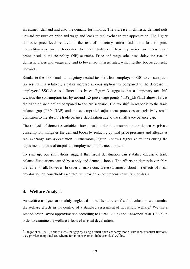
Similar to the TFP shock, a budgetary-neutral tax shift from employers’ SSC to consumption

tax results in a relatively smaller increase in consumption tax compared to the decrease in

employers’ SSC due to different tax bases. Figure 3 suggests that a temporary tax shift

towards the consumption tax by around 1.5 percentage points (TBY_LEVEL) almost halves

the trade balance deficit compared to the NP scenario. The tax shift in response to the trade

balance gap (TBY_GAP) and the accompanied adjustment processes are relatively small

compared to the absolute trade balance stabilisation due to the small trade balance gap.

The analysis of domestic variables shows that the rise in consumption tax decreases private

consumption, mitigates the demand boom by reducing upward price pressures and attenuates

real exchange rate appreciation. Furthermore, Figure 3 shows higher volatilities during the

adjustment process of output and employment in the medium term.

To sum up, our simulations suggest that fiscal devaluation can stabilise excessive trade

balance fluctuations caused by supply and demand shocks. The effects on domestic variables

are rather small, however. In order to make conclusive statements about the effects of fiscal

devaluation on household’s welfare, we provide a comprehensive welfare analysis.

4. Welfare Analysis

As welfare analyses are mainly neglected in the literature on fiscal devaluation we examine

the welfare effects in the context of a standard assessment of household welfare.3 We use a

second-order Taylor approximation according to Lucas (2003) and Canzoneri et al. (2007) in

order to examine the welfare effects of a fiscal devaluation.

3 Langot et al. (2012) seek to close that gap by using a small open-economy model with labour market frictions; they provide an optimal tax scheme for an improvement in households’ welfare.

18

Welfare of household i is given by the discounted sum of the period utilities with the

discount factor :

1 10

0

1( ) ( )

1 1t i i

t tt

W E C L

(27)

As utility has a constant risk aversion , the elasticity of intertemporal substitution is given

by 1/ , specifies the weight on the disutility of work, and 1/ stands for the elasticity of

labour supply. Ricardian (NLC) households as well as rule-of-thumb (LC) households

maximise their utility given their respective budget constraint in equation (1) and (2).

According to Canzoneri et al. (2007), we measure the cost of policy intervention with a

second-order approximation of a value function for aggregate welfare ZW( ) for NLC and

LC households. According to Lucas (2003), ZCC( 0) is a cardinal number defining the

cost of nominal rigidities in percentages of consumption:

Z Z ZCC( 0) W( 0) W( 0) (28)

with

1 1

1 10

( ) ˆˆ( )1 1

( )( ) ˆˆ( ) ( )

2 2

ii i

t tt

Z it i

t t

c lc Ec l El

Wc l

Var c Var l

(29)

The cost of fiscal devaluation ZCC( 0) 4 is given by Z100* 1 (1 )*CC( 0) (see

Canzoneri et al. 2007) and leads to:

Z Z ZCC( 0) 100* 1 (1 ) W( 0) W( 0) (30)

We run simulations over the interval [-10; 2] for the fiscal policy parameter Z in steps of 0.2.

Welfare gains and losses are measured relative to non-stabilisation and are expressed in

percent of steady state consumption for NLC households, LC households and the weighted

4 In the specific case of fiscal devaluation, ZCC( 0) has to be ZCC( 0) in order to simulate a tax shift

from SSC to consumption tax.

19

average of both household types (TOTAL).5 We show welfare gains (positive values) and

welfare losses (negative values) for a range of policy parameter values Z to provide

information on the robustness of welfare effects (see Hohberger et al. 2014). The welfare

effects are simulated for the combination of TFP and risk premium shocks. In order to

attenuate trade balance deficits, fiscal policy aims at increasing net exports by decreasing

employers’ SSC and increasing VAT for consumers, which implies a negative value for the

fiscal policy parameter Z . Hence, a positive parameter value Z implies a tax shift from

VAT to employers’ SSC.

Figure 4 shows that fiscal devaluation leads to welfare losses for NLC and LC households in

the case of stabilising both the trade balance gap (TBY_GAP) and the trade balance in

absolute terms (TBY_LEVEL). Given a fiscal parameter value of Z 10 , fiscal

devaluation generates welfare losses of up to 0.03 % and 0.25 % of steady state consumption

for households average when stabilising TBY_GAP and TBY_LEVEL, respectively.

Figure 4: Welfare effects of fiscal devaluation.

Note: Welfare is measured relative to non-stabilisation and expressed in % of steady state consumption.

Given the identical utility functions for both types of households, the welfare losses for NLC

households are considerably lower compared to LC households as they are able to smooth

5 Similar contributions measuring welfare effects relative to non-stabilisation can be found in Hohberger et al. (2014), Vogel et al. (2013).

-0.07

-0.06

-0.05

-0.04

-0.03

-0.02

-0.01

0

0.01

0.02

-10 -8 -6 -4 -2 0 2 4

%

ξ_Z

Fiscal devaluation (TBY_GAP)

NLC LC TOTAL

-0.5

-0.4

-0.3

-0.2

-0.1

0

0.1

-10 -8 -6 -4 -2 0 2

%

ξ_Z

Fiscal devaluation (TBY_LEVEL )

NLC LC TOTAL

20

their consumption over time. LC households, however, suffer (benefit) more than NLC

households from policy interventions that amplify (stabilise) temporary income fluctuations,

which is line with Hohberger et al. (2014) and Vogel et al. (2013).

In case of TBY_LEVEL stabilisation, a tax shift from SCC to consumption tax generates

welfare losses for LC households up to 0.5 % of steady state consumption as consumption tax

increase reduces purchasing power of disposable period income of LC households. NLC

households experience welfare losses of up to 0.08 % of steady state consumption. NLC

households also experience welfare gains for the policy parameters range [-3; 0]; however,

these welfare gains are negligible small. Increasing prices and higher consumption taxes

encourage NLC households to decrease private consumption in order to maximise their

intertemporal welfare. Furthermore, NLC households smooth their consumption and increase

savings, which immediately leads to an increase in net foreign assets compared to the no-

policy (NP) scenario and, thus, to a decline in the trade balance deficit.

Additionally, as the decrease in consumption demand caused by higher VAT rates counteracts

lower labour and production costs caused by the decrease in SSC, employment remains fairly

stable and, hence, welfare effects are mainly driven by changes in consumption.

5. Sensitivity analysis

This section provides several sensitivity analyses for alternative fiscal closure rules and

distinctions in the tradable and non-tradable sector sizes in order to check the effect of

changes in the model structure. We focus in this section on stabilising the trade balance in

absolute terms (TBY_LEVEL), as stabilising the trade balance gap implies qualitatively

similar welfare effects.

Alternative Budget Closure Rules

As fiscal devaluation is supposed to be budgetary-neutral, deviations from the targeted

government debt/deficit-to-GDP ratio can arise due to output and price changes. For example,

a rise in output after the tax shift reduces government debt-to-GDP ratio, implies a tax

decrease and, hence, a reduction of the crowding-out of private consumption. Therefore, tax

reforms can generate distortionary effects, which influence households’ welfare. Lump-sum

taxes are non-distortionary and therefore considered as efficient taxes, as they do not imply

second-round effects from government debt/deficit stabilisation. They represent immediate

21

government revenues without having additional effects on economic decision-making by

NLC households. In order to gain some intuition about the sensitivity of our welfare results

with respect to alternative budget closures, we modify the model by using labour income and

capital taxes to stabilise government debt and the budget deficit.

Figure 5: Welfare analysis for alternative budget closures

Note: Welfare is measured relative to non-stabilisation and expressed in % of steady state consumption.

Figure 5 depicts that alternative budget closures perform very similarly to lump-sum taxes.

Labour income tax as budget closure induces higher welfare losses for both household types,

while capital tax as closure reduces households’ welfare losses slightly. The overall welfare

performance, however, remains fairly similar.

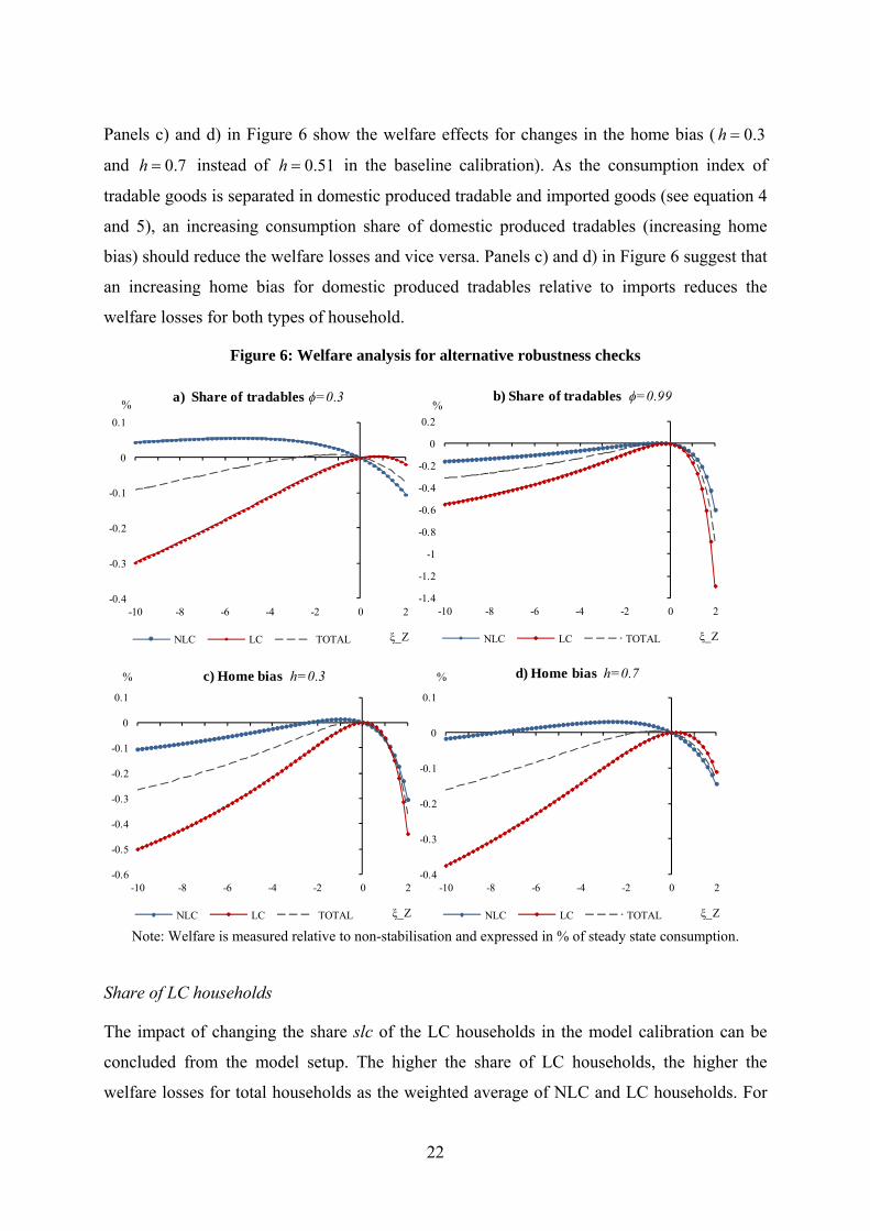
Tradables vs. non-tradables

As fiscal devaluation increases the price for tradable relative to non-tradable goods, the

relative size of both sectors should have an impact on the welfare effects. Panels a) and b) in

Figure 6 depict the welfare effects for tradable goods shares of 0.3 and 0.99 instead

of 0.6 in the baseline calibration. Panels a) and b) suggest that the higher the share of

tradable goods relative to non-tradable goods, the higher the welfare losses for LC and NLC

households. This is due to the fact that a tax shift from SSC to consumption induces non-

tradable goods to become cheaper relative to tradable goods as a composite of domestic

produced and imported goods.

-0.5

-0.4

-0.3

-0.2

-0.1

0

0.1

-10 -8 -6 -4 -2 0 2

%

ξ_Z

Capital Tax Closure

NLC LC TOTAL

-0.7

-0.6

-0.5

-0.4

-0.3

-0.2

-0.1

0

0.1

-10 -8 -6 -4 -2 0 2

%

ξ_Z

Labour Tax Closure

NLC LC TOTAL

22

Panels c) and d) in Figure 6 show the welfare effects for changes in the home bias ( 0.3h

and 0.7h instead of 0.51h in the baseline calibration). As the consumption index of

tradable goods is separated in domestic produced tradable and imported goods (see equation 4

and 5), an increasing consumption share of domestic produced tradables (increasing home

bias) should reduce the welfare losses and vice versa. Panels c) and d) in Figure 6 suggest that

an increasing home bias for domestic produced tradables relative to imports reduces the

welfare losses for both types of household.

Figure 6: Welfare analysis for alternative robustness checks

Note: Welfare is measured relative to non-stabilisation and expressed in % of steady state consumption.

Share of LC households

The impact of changing the share slc of the LC households in the model calibration can be

concluded from the model setup. The higher the share of LC households, the higher the

welfare losses for total households as the weighted average of NLC and LC households. For

-1.4

-1.2

-1

-0.8

-0.6

-0.4

-0.2

0

0.2

-10 -8 -6 -4 -2 0 2

%

ξ_Z

b) Share of tradables ϕ=0.99

NLC LC TOTAL

-0.4

-0.3

-0.2

-0.1

0

0.1

-10 -8 -6 -4 -2 0 2

%

ξ_Z

a) Share of tradables ϕ=0.3

NLC LC TOTAL

-0.4

-0.3

-0.2

-0.1

0

0.1

-10 -8 -6 -4 -2 0 2

%

ξ_Z

d) Home bias h=0.7

NLC LC TOTAL

-0.6

-0.5

-0.4

-0.3

-0.2

-0.1

0

0.1

-10 -8 -6 -4 -2 0 2

%

ξ_Z

c) Home bias h=0.3

NLC LC TOTAL

23

checking the robustness of this assumption, we set slc=0.1 and slc=0.7 with the result that the

separated welfare effects for LC and NLC do not change considerably. However, variations in

the compositions of the two household types induce corresponding changes in welfare of total

households.

6. Conclusion

This paper uses a two-region two-sector DSGE model of a small open economy in monetary

union with nominal and real rigidities to analyse the potential of fiscal devaluation to stabilise

external imbalances. We contribute to the existing literature on fiscal devaluation by

focussing mainly on the effects on households’ welfare. Fiscal devaluation is designed as a

budgetary-neutral tax shift from employers’ social security contribution (SSC) to value-added

tax (VAT). We compare the performance of fiscal devaluation with alternative budget

closures and provide several robustness checks.

The simulation results suggest that fiscal devaluation can stabilise excessive trade balance

fluctuations in absolute terms (TBY_LEVEL). However, the associated tax shift from social

security contribution to consumption tax is accompanied with welfare losses of up to 0.25 %

of steady state consumption for the average household. Thereby, LC households who have no

access to financial markets and cannot smooth their consumption over time suffer more from

a fiscal devaluation with welfare losses of up to 0.5 % of steady state consumption. However,

the welfare losses for both types of households are fairly moderate when stabilising the trade

balance gap. Our findings are robust to several sensitivity checks, i.e. alternative distortionary

budget closures and changes in the relative sector size between tradable and non-tradable

goods.

24

References

Annicchiarico B, Di Dio F, Felici F (2013) "IGEM: A Dynamic General Equilibrium Model

for Italy", Working Papers, No 1.

Auray S, Eyquem A, Ma, X (2014) " Fiscal Devaluations in a Monetary Union and the

Extensive Margin of Trade", CREST Série des documents de travail, No. 2014-11.

Brzoza-Brzezina M, Kolasa M, Makarski K (2013) "Macroprudential policy instruments and

economic imbalances in the euro area", European Central Bank Working Paper Series,

1589.

Canzoneri M, Cumby R, Diba B (2007) "The Cost of Nominal Rigidity in NNS Models",

Journal of Money, Credit and Banking, 39(7), 1563-1586.

de Mooij R, Keen M (2012) "'Fiscal devaluation' and fiscal consolidation. The VAT in

troubled times", IMF Working Paper, 12/85.

DIW Berlin (2014) "Innovation in Greece", Economic Bulletin, 4(10), 12-18.

Druant M, Fabiani S, Kezdi G, Lamo A, Martins F, Sabbatici, R (2009) "How are firms wages

and prices linked. Survey evidence in Europe", European Central Bank Working Paper

Series, 1084.

Engler P, Ganelli G, Tervala J, Voigts S (2014) "Fiscal Devaluation in a Monetary Union",

IMF Working Paper 14/201.

European Union (2013) "Taxation trends in the European Union. Data for the EU member

states, Iceland and Norway", Eurostat statistical books, 2013 ed., Publications Office of

the European Union, Luxembourg.

Galí J (2008) " Monetary Policy, Inflation, and the Business Cycle - An Introduction to the

New Keynesian Framework", Princeton University Press.

Galí J, López-Salido J, Vallés J (2007) "Understanding the effects of government spending on

consumption", in: Journal of the European Economic Association, 5(1), 227-270.

25

Galí J, Monacelli T (2005) "Optimal monetary and fiscal policy in a currency union",

National Bureau of Economic Research Working Paper, 11815.

Gomes S, Jacquinot P, Pisani M (2010) "The eagle. A model for policy analysis of

macroeconomic interdependence in the euro area", European Central Bank Working

Paper Series, 1195.

Hohberger S, Vogel L, Herz B (2014) "Budgetary-Neutral Fiscal Policy Rules and External

Adjustment", Open Economies Review, 25(5), 909-936.

Imbs J, Méjean, I (2010) "Trade Elasticities. A Final Report for the European Commission",

Economic Papers, 432.

Langot F, Patureau L, Sopraseuth T (2012) "Optimal fiscal devaluation", IZA Discussion

Paper No. 6624.

Lipinska A, von Thadden L (2012) "On the (In)effectiveness of Fiscal Devaluations in a

Monetary Union", Finance and Economics Discussion Series.

Lombardo G, Ravenna L (2012) "The size of the tradable and non-tradable sectors. Evidence

from input-output tables for 25 countries", in: Economics letters, 116(3), 558–561.

Lucas R (2003) "Macroeconomic Priorities", American Economic Review, 93(1), 1-14.

Marto R (2013) "Assessing the Impacts of Non-Ricardian Households in an Estimated New

Keynesian DSGE Model", MPRA Paper No. 55647.

Mendoza E (1995) "The Terms of Trade, the Real Exchange Rate, and Economic

Fluctuations", in: International Economic Review, 36(1), 101–137.

Poterba, J, Rotemberg, J, Summers, L (1986): "A tax-based test for nominal rigidities”,

American Economic Review, 76(4), 659–675.

Rabanal P, Aspachs-Bracons O (2009) "The Drivers of Housing Cycles in Spain", IMF

Working Papers 09/203.

Rabanal P, Rubio-Ramírez J (2003) "Comparing New Keynesian Models of the Business

Cycle: A Bayesian Approach", Federal Reserve Bank of Atlanta Working Paper 2001-

22a.

Rabanal P, Tuesta V (2013) "Nontradable Goods and the Real Exchange Rate", Open

Economies Review, 24(3), 495–535.

26

Ratto M, Roeger W, in't Veld J (2009) "QUEST III. An estimated open-economy DSGE

model of the euro area with fiscal and monetary policy", Economic Modelling, 26(1),

222–233.

Simonovska I, Waugh M (2014) "The elasticity of trade: Estimates and evidence", Journal of

International Economics, 92(1), 34-50.

Stähler N, Thomas C (2012) "FiMod – a DSGE model for fiscal policy simulations", in:

Economic Modelling, 29(2), 239-261.

Vogel L, Roeger W, Herz B (2013) "The Performance of Simple Fiscal Policy Rules in

Monetary Union", Open Economic Review, 24, 165–196.