Munich Personal RePEc Archive Is inflation targeting the proper monetary policy regime in a dual banking system? new evidence from ARDL bounds test Ndiaye, Ndeye Djiba and Masih, Mansur INCEIF, Malaysia, INCEIF, Malaysia 12 May 2017 Online at https://mpra.ub.uni-muenchen.de/79420/ MPRA Paper No. 79420, posted 27 May 2017 23:25 UTC
Transcript
Munich Personal RePEc Archive
Is inflation targeting the proper
monetary policy regime in a dual
banking system? new evidence from
ARDL bounds test
Ndiaye, Ndeye Djiba and Masih, Mansur
INCEIF, Malaysia, INCEIF, Malaysia
12 May 2017
Online at https://mpra.ub.uni-muenchen.de/79420/
MPRA Paper No. 79420, posted 27 May 2017 23:25 UTC
Is inflation targeting the proper monetary policy regime in a dual
banking system? new evidence from ARDL bounds test
Ndeye Djiba Ndiaye1 and Mansur Masih2
Abstract
This paper explores the appropriateness and consequently the feasibility of inflation
targeting in an economy with a dual financial system. We take the case of Malaysia,
an example of a successful coexistence of the conventional and Islamic systems.
The study employs ARDL bounds testing approach to investigate the long run
relationship between inflation rate, real effective exchange rate, statutory reserve
rate, narrow money, Islamic interbank rate and the overnight policy of Malaysia,
considering the major transmission mechanism channels in the conduct of monetary
policy stance. An Error Correction Model (ECM) is used to capture the short run
dynamics, and variance decomposition of forecast errors is used to determine the
causality direction of the variables. The periods considered was monthly data from
the June 2007 to February 2017. Our results show that there is a long and short term
relationship between inflation, narrow money, statutory reserve rate, real effective
exchange rate and the Islamic interbank rate. However, we suggest that Inflation
targeting may not be ideal in a dual banking system, especially the case of Malaysia.
Alternatively, interest rate targeting is found to be most effective. Additionally, it
will give the central bank more control over the Islamic segment of the financial
1Graduate student in Islamic finance at INCEIF, Lorong Universiti A, 59100 Kuala Lumpur, Malaysia.
2 Corresponding author, Professor of Finance and Econometrics, INCEIF, Lorong Universiti A, 59100 Kuala Lumpur, Malaysia. Phone: +60173841464 Email: [email protected]
1. Introduction
There has been witnessed an increasing number of central banks, from both developed
countries and emerging market economies, implementing inflation targeting since 1990s.
Inflation targeting is a monetary policy that uses the announced inflation targets as a nominal
anchor. Central banks who adopt inflation targeting tend to stress on the importance of pursuing
monetary policy framework to achieve low inflation (Poon, 2009). The central bank then sets
a path for the policy instrument to achieve the target inflation rate.
In the mid-1990s BNM abandoned monetary targeting and switched to an interest rate
targeting, arguing that the relationship of a monetary aggregate with the final objective of price
stability had become difficult to predict given the effects of financial liberalization and
innovation. This had become especially evident in the early 1990s, when large amounts of
capital flowed into Malaysia’s financial markets. In practice, BNM’s monetary strategy now appears to lean very much towards an inflation-targeting regime (Hill, et al., 2012).
However, the case of Malaysia is particular as the country has a dual banking system. The implementation of monetary policy and the transmission mechanism of monetary policy within such system is a challenge for the central bank of Malaysia (BNM). Indeed, unlike in conventional monetary policy, implementing market-based monetary policy in Islamic banking systems, which are based on interest-free assets, is unique and complex. The complexity derives from the challenges in designing a market-based instrument that satisfies the Islamic prohibition on interest payments and provides for sharing both profits and losses in the interest of monetary control and government financing (Muhamed Zulkhibri, 2016). The challenges
arise not only from the Islamic finance core principles but also from the macro financial background and the monetary policy frameworks of countries where Islamic banks operate. As in conventional systems, monetary policy in the presence of Islamic banking needs to be adequately address. However, the central bank’s (CB) capacity to influence market conditions varies significantly (Khatat, 2016).
Indeed, monetary policy affects economic activity and inflation through numerous channels, usually referred to as the transmission mechanism. In a conventional economic system, changes in the immediate instrument of policy, the official interest rate, affect market interest rates, which in turn affect households’ spending and saving plans by altering the mortgage rate and the cost of consumer credit and firms’ investment and borrowing decisions by altering the cost of capital. In an open economy, other things being equal, changes in the official rate also tend to produce changes in the value of the domestic currency vis-à-vis other currencies. By influencing the competitiveness of domestic exports and imports, this affects net trade and hence aggregate demand. In addition, because some of the goods consumed
domestically are imported, changes in the exchange rate usually also have direct effects on consumer price inflation. However, when there are multiple channels of monetary transmission, especially in the case of a dual banking system, it may be desirable to consider as many channels as possible to evaluate the general stance of monetary policy, especially those
directly related to the Islamic financial institutions like the Islamic interbank money market rates.
In addition, there are other transmission channels that may have a direct and non-negligible impact on the inflation rate, such as, for instance, the exchange rate via its direct effect on prices. Recently, against a background in which several factors have contributed to higher attention being granted to stock market developments in monetary policy forecasts and analysis, some indices have been calculated additionally including prices of other financial assets, as well as stock prices. In fact, in some countries such as the United States, stock prices seem to play an important role in the monetary policy transmission mechanism, through wealth
effects and effects on the structure of the balance-sheets of the households, corporations and financial intermediaries (Costa, 2000).
All of the above leads to the overarching question as to if inflation rate the proper monetary target in a dual banking system?
The central objective of this paper is to determine if inflation is the proper monetary policy target in a dual banking system and main monetary transmission channels in such a system. To do so, we will use standard time series technique.
In light of the increasing number of central banks implementing inflation targeting since 1990s, many studies have been conducted to examine the matter, but only a few studies have been conducted on a dual banking system country. Our study contributes to the literature in this direction as we kick it up a notch by specifically adding Islamic channels to our analysis. Our study fills the gap in examining the proper monetary target in a dual banking system. This to our knowledge hasn’t been done before. It would be of paramount importance for any policy maker in a dual banking system to determine the most effective monetary target. We will focus on Malaysia because of its successful implementation of a dual banking system.
The remainder of the paper is organized as follows: Section 2 discusses the theoretical and empirical literature. Section 3 describes the data, variables and methodology. Section 4 presents the empirical results and discusses the findings. Section 5 concludes the study and offers policy implications with suggestions for future research.
2. Theoretical Framework
Inflation targeting is a monetary-policy strategy that was introduced in New Zealand in 1990. New Zealand had experienced high and volatile inflation in the 1970s and the early 1980s. Monetary policy was tightened and inflation fell in the latter part of 1980s. The Reserve Bank Act of 1989 established inflation targeting as a policy framework to solve the issue. The key aspects of the framework were the central bank independence, the accountability of the central bank and an inflation target for monetary policy.
In reality, the implementation of inflation targeting is never “strict” but always “flexible”. Indeed all inflation-targeting central banks not only aim at stabilizing inflation around the inflation target but also put some weight on stabilizing the real economy. For instance, implicitly or explicitly they thrive to stabilize some measures of resource utilization such as the output gap between actual output and potential output.
Thus, the target variables of the central bank include not only inflation but other variables as well, such as the output gap. The objectives under flexible inflation targeting seem well approximated by a quadratic loss function consisting of the sum of the squared inflation deviation from target and a weight times the squared output gap, and possibly also a weight times the squared policy-rate change (the last part corresponding to a preference for interest-rate smoothing). Because there is a lag between monetary-policy actions (such as a policy-rate
change) and its impact on the central bank’s target variables, monetary policy is more effective if it is guided by forecasts.
Therefore, the implementation of inflation targeting gives a main role to forecasts of
inflation and other target variables. It can be described as forecast targeting, that is, setting the policy rate (more precisely, deciding on a policy-rate path) such that the forecasts of the target variables conditional on that policy-rate path stabilize both inflation around the inflation target and resource utilization around a normal level. Because of the clear objective, the high degree of transparency and accountability, and a systematic and elaborate decision process using the most advanced theoretical and empirical methods as well as a sizeable amount of judgment, inflation targeting provides stronger possibilities and incentives to achieve optimal monetary policy than previous monetary-policy regimes (Svensson, 2010).
Indeed, conceptually, inflation targeting is very appealing and most studies theorize a positive effect of inflation targeting in a country’s macroeconomic performance. According to Mishkin (2001), inflation targeting has several advantages as a medium-term strategy for monetary policy. In contrast to an exchange rate peg, inflation targeting enables monetary policy to focus on domestic considerations and to respond to shocks to the domestic economy.
Contrary to monetary targeting, another possible monetary policy strategy, inflation targeting has the advantage that a stable relationship between money and inflation is not critical to its success: the strategy does not depend on such a relationship, but instead uses all available information to determine the best settings for the instruments of monetary policy. Inflation targeting also has the key advantage that it is easily understood by the public and is thus highly
transparent. Because an explicit numerical target for inflation increases the accountability of the central bank, inflation targeting has the potential to reduce the likelihood that the central bank will fall into the time-inconsistency trap.
Moreover, since the source of time-inconsistency is often found in (covert or open) political pressures on the central bank to undertake overly expansionary monetary policy, inflation targeting has the advantage of focusing the political debate on what a central bank can do in the long-run -- i.e., control inflation -- rather than what it cannot do -- raise output growth, lower unemployment, increase external competitiveness-- through monetary policy (Mishkin, 2001).
In contrast to that mentioned above, (Friedman, 2004) offers arguments against the implementation of inflation targeting by central banks. Friedman urged that there is no empirical evidence to the value added by inflation targeting in terms of a country’s macroeconomic performance. Friedman goes further as to deny the claims commonly made that conceptually inflation targeting usefully enhances the transparency of monetary policy. He argued that as actually practiced, inflation targeting is a framework not for communicating the central bank’s goals but for obscuring them. He adds that by forcing participants in the monetary policy debate to conduct the discussion in a vocabulary pertaining solely to inflation,
inflation targeting fosters over time the atrophying of concerns for real outcomes. In the meanwhile, inflation targeting hides from public view whatever concerns for real outcomes policy makers do maintain, thereby not fostering transparency in policy making but undermining it and this is not consistent with the role we should seek for monetary policy in a democracy.
Moreover (Calvo, 1999) showed that inflation targeting under imperfect credibility could produce distortionary effects similar to those encountered in non-fully-credible fixed exchange rate regimes. Consequently, non-credible inflation-target programs may suffer from much the same maladies that afflict non-credible currency pegs. Moreover, readers familiar with the
earlier literature will notice that non credible inflation target programs give rise to richer consumption and real exchange rate dynamics than non-credible currency pegs.
Intuitively, the success of inflation targeting regime depends largely on the central bank independence, the degree of central bank accountability and transparency to the public, the
relationship between inflation and the instruments of monetary policy, the explicit institutional commitment of the monetary authority to focus on price stability as its primary implicit and explicit goals of the policy, the development of models that allows the monetary authority to incorporate transmission mechanisms in the economy, the setting appropriate channels of communication between the monetary authority and economic agents, and the mechanism to make the authority accountable for the outcomes (Mishkin & Savastano, 2001).
Incorporating Islamic banks in the monetary policy framework is a complex task not only because of the need of compliance with Islamic finance core principles but also due to the heterogeneity of financial systems and monetary policy frameworks of countries where Islamic banking exists (Khatat, 2016). The theoretical effects of inflation targeting are mixed. Thus, whether inflation targeting is the right monetary policy target in a dual banking system or specifically for Malaysia will need to be answered empirically.
3. Empirical Literature
Furtherance to the theoretical underpinnings, several empirical studies have been documented on inflation targeting countries. Empirically, the results of the effect of inflation targeting in a country’s macroeconomic performance are mixed.
Indeed, (Thornton & Vasilakis, 2017) assessed whether the adoption of inflation targeting frameworks has facilitated countercyclical monetary policies in a sample of 90 industrial and developing economies, 22 of which have adopted inflation targeting. Using propensity score matching methods, they showed that inflation targeting has a statistically significant and quantitatively quite large effect in facilitating a more countercyclical monetary policy in inflation targeting countries.
Moreover, Wu (2004) found evidence of the causal effect of a country's adoption of the Inflation Targeting regime on that country's inflation rate decline. He used quarterly CPI inflation rates of 22 OECD countries for the period of 1985-2002, and found that countries that have officially adopted Inflation Targeting experience a decrease in their average inflation
rates. He also found that there seems to be no evidence that Inflation targeting countries experienced a significant increase in the level of their real interest rates after they adopted the
new regime and that even after controlling for the level of real interest rates there is still a causal effect from the adoption of Inflation Targeting to the reduction in inflation rates. He rejects the idea that the better performance in the inflation rates of the Inflation targeting countries is only due to a more "aggressive" monetary policy.
Similarly, (Lee & Poon, 2014) investigated the applicability of inflation targeting in ASEAN countries, focusing on the role of the real exchange rate and exchange rate volatility, and the central banks’ reaction functions. Their results illustrate that both inflation targeting and non- inflation targeting ASEAN countries response significantly to inflation gap; but neither inflation targeting nor Non- inflation targeting groups respond significant to the output
gap in setting the interest rates. Comparatively, the role of real exchange rate is more significant in Non- inflation targeting countries than in inflation targeting countries. Inflation targeting countries appear to follow a “mixed strategy” as both inflation and real exchange rate are important determinants when it comes to setting of interest rates. Results demonstrate that inflation targeters have lower exchange rate volatility compared to non-inflation targeters, which implies that inflation targeting does not seem to come as a “cost” to domestic economy with respect to higher exchange rate volatility.
While macroeconomic experiences among both inflation targeting and non-inflation targeting developed economies have been similar, inflation targeting has improved macroeconomic performance among developing economies. Importantly, there is no evidence that inflation targeting has been detrimental to growth, productivity, employment, or other measures of economic performance in either developed and developing economies. Inflation targeting has stabilized long-run inflation expectations.
In contrast, (Cecchetti & Ehrmann, 1999) found that Inflation targeting made little difference. They studied whether inflation targeting increase output volatility in 23 industrialized and developing economies, including nine that target inflation explicitly. Their results suggest that both countries that introduced inflation targeting, and non-targeting European Union countries suffered increases in output volatility. However they conclude that
the inflation targeters increased their aversion to inflation volatility by more than the nontargeters, although the difference is modest. In addition, (Ball & Sheridan, 2003) compared seven OECD countries that adopted inflation targeting in the early 1990s to thirteen non-targets. They found there no evidence that inflation targeting improves economic performance.
Specifically, for Malaysia, the focus of our study, Poon and Tong (2009) previously investigated the feasibility of inflation targeting in Malaysia, applying the Johansen-Juselius (JJ) multivariate cointegration procedure and Vector Error Correction Modelling (VECM). They found cointegration between CPI and exchange rate, money market rate, and money supply. Their results show that changes in interest rate and exchange rate have significantly impacted the CPI in Malaysia in the short run. However they concluded that inflation targeting may not fit in Malaysia because of its economic structure and institution may not be conducive at the current stage. Their time series data was from 1976:M1 to 2007:M12. Indeed Mishkin (2004) stresses that to ensure that inflation targeting produces superior macroeconomic outcomes, emerging market countries would benefit by focusing even more attention on
institutional development. He goes further as to lay out the two underlying monetary institutions that are necessary for the ability of the monetary authorities for the success of inflation targeting. The first is a public and institutional commitment to price stability as the
overriding long-run goal of monetary policy. The second is a public and institutional commitment to instrument independence of the central bank. Does Malaysia fill these two conditions is up for further study.
4. Data and Empirical Estimation
4.1. Data
This study aimed to investigate whether inflation rate is the proper monetary policy target in Malaysia. We analyzed the relationship between the main transmission mechanism channels in the conduct of monetary policy stance in a conventional system and experiment with the channels through which the central bank (CB) can control the Islamic financial sector.
The definitions of all the variables in this paper are presented in Table 1. The monthly data from June 2007 to February 2017 was sourced from Datastream, the BNM website and Bloomberg database.
Table1: Variables and Data Definitions
Variable Definition
Inflation (Consumer Price Index as
proxy)
Inflation is the rising price of goods and services over time. The cost of living
increases. The inflation rate is the percent increase or decrease of prices during a specified period. The U.S. Bureau of Labor Statistics (BLS) uses the Consumer
Price Index (CPI) to measure inflation. The CPI will tell you the general rate of inflation (Amadeo, 2016)
Real Exchange Rate
The real exchange rate R is defined as the ratio of the price level abroad and the
domestic price level, where the foreign price level is converted into domestic currency units via the current nominal exchange rate. Formally, R=(E.P*)/P, where the foreign price level is denoted as P* and the domestic price level as P
(CNB, 2017).
Narrow money
Narrow money is a category of money supply that includes all physical money like coins and currency along with demand deposits and other liquid assets held by the
central bank. In the United States, narrow money is classified as M1 (M0 + demand accounts), while in the U.K., M0 is referenced as narrow money
(Investopedia, 2017).
Output Gap
The output gap is an economic measure of the difference between the actual output of an economy and its potential output. An important determinant of inflation is the
relationship between the overall level of demand for goods and services in the economy and the capacity of the economy to supply them (output gap).
Potential output is the maximum amount of goods and services an economy can turn out when it is most efficient—that is, at full capacity. Often, potential output is
referred to as the production capacity of the economy. Policymakers often use potential output to gauge inflation and typically define it as the level of output
consistent with no pressure for prices to rise or fall. In this context, the output gap is a summary indicator of the relative demand and supply components of economic
activity. As such, the output gap measures the degree of inflation pressure in the economy and is an important link between the real side of the economy—which produces goods and services—and inflation. All else equal, if the output gap is
positive over time, so that actual output is greater than potential output, prices will begin to rise in response to demand pressure in key markets. Similarly, if actual
output falls below potential output over time, prices will begin to fall to reflect weak demand (Jahan & Mahmud, 2013).
Statutory Reserve
Requirement (Reserve
Balance or Required
Reserve Requirement)
for Islamic Banks
SRR Rate
The Statutory Reserve Requirement (SRR) is a monetary policy instrument
available to Bank Negara Malaysia (the Bank) for purposes of liquidity management. Effectively, banking institutions are required to maintain balances in their Statutory Reserve Accounts (SRA) equivalent to a certain proportion of their
eligible liabilities (EL), this proportion being the SRR rate (BNM, 2016).
Overnight Policy Rate
OPR is the interest rate/profit rate at which a bank lends to/receives from investment with another bank. OPR is determined by Bank Negara Malaysia in the Monetary Policy Committee
Meeting held throughout the year (CIMB, 2017). Overnight Policy Rate (OPR) is an overnight interest rate set by Bank Negara.
Islamic Interbank Rate
Islamic interbank rate is the daily weighted average rate of the Mudharabah
interbank investment at the IIMM in Kuala Lumpur, where the individual rates being weighted accordingly by the volume transactions at those rates (BNM,
2017).
Another variable that we considered is the base financing rate (BFR), a rate determined by Islamic financial institutions based on the cost of financing to consumers. Because OPR changes will directly influence BFR revisions (CIMB, 2017), we decided not to include BFR as a variable because of the direct link between BFR and OPR. In addition, the output gap and unemployment gap could not be included in our variables for lack of data. Our study will consist of the six variables shown in table 2 below.
Table 2: Variables, symbols, sources of data collection and reference
This study aimed to investigate whether inflation targeting is the proper monetary policy target in Malaysia during the period 2007-2017, by applying the Autoregressive Distributed Lag model (ARDL) analysis by using six variables based on previous studies and our research objective. We explored the long run equilibrium relationship between a set macroeconomic indicators and financial variables (inflation rate, the OPR, REER, SRR, narrow money and IRR) using ARDL bounds testing approach.
In fact, in testing the relationship between inflation and the other variables, regression will not answer our query, as regression assumes causality. Our aim is to determine the direction of causality between inflation and the other variables studied. By answering this we can conclude whether inflation is the proper monetary policy target in a dual banking system, in this case Malaysia. Additionally we will be able to determine the adequate transmission channels to influence the proper monetary target. This is the reason why we are using time series technique not regression. Regression assumes theoretical relationship between variables but time series tests the theoretical relationship between variables through cointegration tests. Thus, time series technique is more adequate for the purpose of our study.
More so, most empirical studies apply Engle-Granger or Johansen method for studying cointegration, but in our case, both Engle-Granger and Johansen methods are not suitable, since our time series are small and our variables in the series are not of the same order (i.e. we have a mixture of I(0) and I(1) series).
On the other hand, ARDL methodology for testing cointegration is superior to earlier approaches such as Engle-Granger or Johansen. It can be applied to situations where the
variables have different orders of integration, and where the time series are short. The earlier approaches, on other hand required all series to be integrated of the same order. Moreover, ARDL gives robust results even in small samples, which is a major advantage when the available time series are small, as they typically are in many emerging economies (Faiza Abbasi, 2016).
The standard ARDL technique has two stages. First, investigation of the existence of a long-run relationship among variables. This is done by constructing an unrestricted error correction model (VECM) with each variable in turn as a dependent variable and then testing whether or not the ‘lagged levels of the variables’ in each of the error correction equations are statistically significant (i.e., whether the null of ‘no long run relationship’ is accepted or rejected).
Basically, the ARDL method is the Wald test (F-statistic version of the bounds testing approach) for the lagged level variables in the right-hand side of VECM. That is, we test the null hypothesis of no cointegrating relation (Ho: b1= b2= b3=...= bn=0) by performing a joint significance test on the lagged level variables. The asymptotic distribution of the F- statistic is non-standard under the null hypothesis of no co-integrating relation between the examined variables, irrespective whether the explanatory variables are purely I(0) or I(1). The test consists of computing an F-statistic testing the joint significance of the ‘lagged levels of the variables’ in each of the above error-correction form of the equation. The computed F-statistic is then compared to two asymptotic critical values. If the test statistic is above an upper critical value, the null hypothesis of ‘no long-run relationship’ can be rejected regardless of whether
the variables are I(0) or I(1). Alternatively, when the test statistic falls below a lower critical value, the null hypothesis of ‘no long-run relationship’ is accepted regardless of whether the variables are I(0) or (1).
Finally, if the test statistic falls between these two bounds, the result is inconclusive. It is only in this case that the researcher may have to carry out unit root tests on the variables. As regards the implications of the F-statistics, if all the F- statistics in all equations happen to be insignificant, then that implies the acceptance of the null of ‘no long run relationship’ among the variables. However, if at least one of the F-statistics in the error- correction equations is significant, then the null of ‘no long-run relationship’ among the variables is rejected. In that case there is a long run relationship among the variables. When the F-statistic is significant, the corresponding dependent variable is endogenous and when the F-statistic is insignificant, the corresponding dependent variable is exogenous or called ‘long-run forcing variable’ (Mustapha & Masih, 2016).
The ARDL model specifications of the functional relationship between inflation (INF), real effective exchange rate (REER), statutory reserve rate (SRR), narrow money (M), Islamic interbank rate (IRR), and overnight policy rate (OPR) can be estimated below:
+ 𝛿6𝑂𝑃𝑅𝑡−1 + 𝜀𝑡 Once the long run relationship has been demonstrated, the second stage of the analysis
involves the estimation of the long run coefficients (after selecting the optimum order of the variables through AIC or SBC criteria) and then estimate the associated error correction model in order to estimate the adjustment coefficients of the error-correction term. If there is a long term relationship among the variables, then the ARDL analysis generates the ECM equation for every variable, which provides information through the estimated coefficient of the error correction term about the speed at which the dependent variable returns back to equilibrium once shocked (Mustapha & Masih, 2016).
The error-correction model also indicates the absolute the endogeneity/exogeneity of a
variable. However, to determine the relative endogeneity/exogeneity of each variable, we apply the generalized variance decomposition technique. Through VDCs, the relative exogeneity/endogeneity of a variable can be determined by the proportion of the variance explained by its own past. The variable that is explained mostly by its own shocks (and not by others) is deemed to be the most exogenous.
Following the above, impulse response functions (IRFs) will be used to map out the dynamic response path of every variable due to a one-period standard deviation shock to another variable. The IRF is a graphical way of exposing the relative exogeneity or endogeneity of a variable. Finally, we will present the persistence profile. It is designed to estimate the speed with which the variables get back to equilibrium when there is a system wide shock to the cointegrating relationship (long-run equilibrium) (Masih, Al-sahlawi, & Mello, 2010).
5. Findings and Interpretations
Before proceeding with the ARDL framework, we examined the unit roots of the variables. Even though the bounds test for cointegration does not require a pre-testing of the variables for unit root, but it can ascertain our scepticism whether or not ARDL modelling is required in the first place. It is also imperative that this test is conducted to ensure that our series are not
integrated of an order higher than one, otherwise our study may suffer the problem of spurious results.
Unit Root Tests
We have employed the Augmented Dickey-Fuller (ADF) tests to determine Stationarity, and we employed the Schwartz-Bayesian Criterion (SBC) and Akaike Information Criterion (AIC) to determine the optimal number of lags included in the test. The results of the ADF test are reported in Table 3. Table 3: Unit Root Tests
All the variables are transformed into logarithms to achieve stationarity in variance. The presence of non-stationary behavior in the autoregressive representation of the variable is determined by the Augmented Dickey-Fuller (ADF) unit root test. The result shows that on one hand, all our log-transformed variables are non-stationary except from inflation. And on the other hand, all our difference-transformed variables are stationary.
UNIT ROOT TESTS
1S
T D
IFF
. F
OR
M
VARIABLE ADF VALUE T-STAT. C.V. RESULT
DINF ADF(1)=SBC 427.7169 -6.336 -2.888 Stationary
ADF(1)=AIC 431.7677 -6.336 -2.888 Stationary
DREER ADF(1)=SBC 303.2956 -7.11 -2.888 Stationary
ADF(1)=AIC 307.3463 -7.11 -2.888 Stationary
DSRR ADF(1)=SBC 87.8217 -5.723 -2.888 Stationary
ADF(1)=AIC 91.8724 -5.723 -2.888 Stationary
DM ADF(1)=SBC 269.2142 -10.6 -2.888 Stationary
ADF(3)=AIC 274.8795 -7.551 -2.888 Stationary
DIIR ADF(1)=SBC 210.4626 -5.302 -2.888 Stationary
ADF(1)=AIC 214.5133 -5.302 -2.888 Stationary
DOPR ADF(1)=SBC 197.555 -5.201 -2.888 Stationary
ADF(1)=AIC 201.6057 -5.201 -2.888 Stationary
Since our variables are confirmed to be a mixture of I(0) and I(1) using ADF test, we can now proceed with the cointegration test using the ARDL technique to test the long run relationship among the variables.
However, before proceeding with the test of cointegration, we try to determine the order
of the vector auto regression (VAR), Even though it is not necessary to find out the VAR order for the ARDL approach since the process itself find individual lag order to each variable. It would be interesting to find coherence between the VAR lag order selection and the ARDL individual lag order selection. Table 4 below, shows the optimal order of the VAR based on both Akaike information criterion (AIC) and Schwarz Bayesian Criterion (SBC) is to the order of 1. Table 4: VAR Lag Order Selection
Optimal VAR lag Order AIC SBC p-Value C.V.
1 1607 1550.3 [.362] 5%
Testing for Cointegration
Cointegration implies that there is co-movement of the variables and that they are in
equilibrium in the long run. When you have more than two variables in the model, there is a possibility of having more than one cointegrating vector. Our results reveal that there are three sub-groups among the variables which are moving together.
We applied ARDL bound testing to test for the existence of a long-run relation relations by computing the F-statistic for testing the significance of the lagged levels of the variables in the error correction form of the underlying ARDL model. The results of the bound test are given in Table 5, where we found two cointegration vectors at 95-percent significance level. The null hypothesis of zero cointegrating vector is rejected at 5-percent significance level, based on the critical values extracted from Pesaran et al. (2001). Table 5: F-Statistics for testing the Existence of Long-Run Relationship (Variable Addition Test)
Variables F-stat L. Bound 95% U. Bound 95% Relationship
From the table above, we find that when inflation is the dependent variable, the
calculated F-statistic 𝐹𝐿INF (LINF | LREER, LSRR, LM, LIIR, LOPR) =6.5084 is higher than
the upper bound of the critical value obtained from Pesaran et al. (2001), indicating there is a
significant evidence for cointegration between inflation and the other variables for the study
period. However, the evidence of long run relationship rules out the possibility of any spurious
relationship existing between the variables. In other words, there is a theoretical relationship
existing between the variables. The process has been repeated for the other variables and result
shows that OPR indicates compelling evidence of long run relationship with the other
determinants.
The evidence of a cointegrating relationship implies that there is a common force that
brings INF, REER, SRR, M, IIR and OPR together in the long run. It confirms that there is a
theoretical relationship between the variables. Cointegration implies that these variables are
interdependent and highly integrated.
As stated earlier, cointegration tells us that there is a long run relationship between the
variables. However, the possibility of a short-run deviation from the long-run equilibrium
cannot be ruled out. Cointegration does not unfold the process of short-run adjustment to bring
about the long-run equilibrium. Also, cointegration cannot tell us the direction of causality
between the variables as to which variable is leading and which variable is lagging. For
understanding that adjustment process, and the absolute endogeneity/exogeneity of the
variables, we need to go to the ARDL error-correction model.
Error Correction Model of ARDL
In the following table, the ECM’s representation for the ARDL model is selected with AIC Criterion and SBC criterion. The result of our error correction model estimates are found to be consistent, irrespective of the criterion involved.
Table 6: Error Correction Model of ARDL
Akaike Information Criterion
ecm1(-1) Coefficient Standard Error T-Ratio [Prob.] Significance C.V. Result
The T-ratio or the p-value of the error correction coefficient indicates whether the deviation from equilibrium (represented by the error correction term, ‘ecm’) has a significant feedback effect or not on the dependent variable. In other word, whether the variable is endogenous or exogenous. The error-correction coefficient being significant confirms our earlier findings of a significant long run Co-integrating relationship between the variables. Also, the coefficient of the error-correction term indicates the speed of short run adjustment of
the dependent variable to bring about the long run equilibrium. The size of the coefficient of the error-correction term is also indicative of the intensity of the arbitrage activity to bring about the long-run equilibrium (Mustapha & Masih, 2016).
Looking at the significance or otherwise of the coefficient of the error correction term,
we find that the narrow money variable is the only exogenous variable, whereas the other variables, INF, REER, SRR, IIR, and OPR are endogenous. This indicates that the narrow money is the driver and that inflation responds to the monetary variable. The error-correction term in the inflation equation is significant. This implies that the deviation of the variables (represented by the error correction term) has a significant feedback effect on the inflation variable that bears the burden of short-run adjustment to bring about the long-term equilibrium. In the short run all the variables have a significant effect on each other except for narrow money which is not affected by the other variables in the short run.
Additionally, the error-correction model also helps us distinguish between the short-term and long-term Granger causality. The error-correction term stands for the long-term relations among the variables. The impact of each variable in the short term is given by the ‘‘F’’ tests of the joint significance or insignificance of the lags of each of the ‘‘differenced’’ variables. The speed of short-run adjustment to bring about the long term equilibrium is given by the coefficient of the error-correction term. The diagnostics of all the equations of the error-
correction model (testing for the presence of serial correlation, functional form, normality, and heteroscedasticity) tend to indicate that the equations are more or less well-specified.
After considering the INF (Inflation) as the dependent variable, as mentioned in the objectives of the paper, it is indeed to spot the impact of our variables set on INF (Inflation) in short run and in long run. The following empirical results show the nature of the impact of our variables set in short and long run on INF (Inflation).
Although the error correction model indicates the endogeneity/exogeneity of a variable,
it does not indicate the relative endogeneity or exogeneity of each variables, nor do they allow
us to gauge the relative strength of the granger-causal chain or degree of exogeneity amongst
the variables beyond the sample period. Consequently, we need apply the variance
decomposition techniques (VDCs) to discern the relative degree of endogeneity or exogeneity
of each variable. VDCs by partitioning the variance of the forecast error of a certain variable
into proportions attributable to shocks in each variable in the system including its own, can
provide an indication of these relativities. A variable that is optimally forecast from its own
lagged values will have all its forecast error variance accounted for by its own disturbances
(Sims, 1982).
Variance Decompositions (VDC)
VDCs can give us information about relative exogeneity/endogeneity, for example,
identify which variable is most exogenous, which one is the most endogenous. The
orthogonalized VDCs are not unique and in general depend on the particular ordering of the
variables in the VAR but the generalized VDCs are invariant to the ordering of the variables.
The orthogonalized VDCs assumes that when a particular variable is shocked, all other
variables in the model are switched off but the generalized VDCs do not make such a
restriction. The relative exogeneity or endogeneity of a variable is determined by the proportion
of the variance explained by its own past (Domingos, 2000). The analysis aims at calculating
the contribution of innovations to the forecast-error variance. To that effect, we express the
individual forecast-error variance to a given horizon in function of the error variance assigned
to each variable in the system in order to obtain the relative importance in percentage.
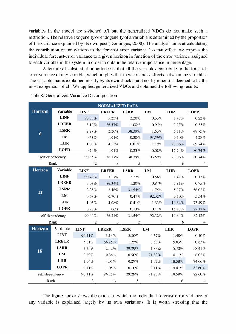
A feature of substantial importance is that all the variables contribute to the forecast-
error variance of any variable, which implies that there are cross effects between the variables. The variable that is explained mostly by its own shocks (and not by others) is deemed to be the most exogenous of all. We applied generalized VDCs and obtained the following results:
The figure above shows the extent to which the individual forecast-error variance of
any variable is explained largely by its own variations. It is worth stressing that the
contributions are higher for the variables at the earlier periods than the later horizons except
for inflation and OPR.
Similarly, it can be seen that in the 6 months’ horizon, we find that 90.35 percent of the
forecast error variance of inflation is explained by its own shocks. Since 90.35% of the
variation in inflation is explained by its own past then using inflation to target other variables
would be more efficient than using other variables to target inflation. This implies that using
inflation as the ultimate target of monetary policy may not be most effective.
In the case of real effective exchange rate the proportion that is explained by its own
shock is also high as 86.57 percent. While, the statutory required reserve, the Islamic interbank
rate and overnight policy rate variables, each of them is explained by its own shock respectively
by 38.39, 23.06, 80.74 percent of the forecast error variance of each variable is explained by
its own shocks. But in the case of the narrow money variable, 93.59 percent of the forecast
error variance of that variable is explained by its own shocks. That tends to indicate that the
narrow money variable is the most exogenous. IRR is the most endogenous followed by SRR,
OPR, REER and INF respectively.
The fact the direction of causality goes from narrow money to inflation seems to be in
accordance with monetarists’ view that inflation is always and everywhere a monetary phenomenon (Friedman, 1966).
Up to the 18 months horizon, IIR still remained the most endogenous and the other
variables kept their ranking. In the short and medium term, SRR and OPR remained the most
endogenous and remained so in the long run. While REER, INF and M remained the third,
second and most exogenous variable respectively. They remained leader over the 10 years
period of study.
Our results show that there is a long term relationship between inflation, OPR, SRR,
REER, M and IIR in the long and short run. Inflation targeting may not be the proper monetary
policy target for Malaysia. This is in line with the results of Poon and Tong (2009) who
previously investigated the feasibility of inflation targeting in Malaysia applying the Johansen-
Juselius (JJ) multivariate cointegration procedure and Vector Error Correction Modelling
(VECM). They found cointegration between CPI and exchange rate, money market rate, and
money supply. Their results show that changes in interest rate and exchange rate have
significantly impacted the CPI in Malaysia in the short run. However they concluded that
inflation targeting may not be fit in Malaysia because of its economic structure and institution
may not be conducive at the current stage.
Moreover, our results suggest that interest rate targeting may be the proper monetary
policy target for Malaysia and that inflation rate, real effective exchange rate and narrow money
could be used as intermediate target. Moreover, since OPR changes directly influence BFR and
BLR revisions (CIMB, 2017), and our results show that OPR has an effect on the Islamic
interbank rate, if Malaysia targets the interest rate it would be able to have more control of the
Islamic segment of the financial system. BNM would be able affect the supply of Islamic credit
through the OPR. In addition our result show that BNM through OPR can influence the funding
costs of Islamic banks by targeting the Islamic interbank rate, as it has been proven to be the
most endogenous variable in the relationship.
Indeed, as Khatat (2016) argued, introducing Islamic banks in macrofinancial
environments where the interest rate channel is well established can result in conventional
monetary policy transmission through the Islamic financial system, even if this transmission
has not been anticipated by the CB. Because financial systems where Islamic banking is
systemic are typically dual and not fully developed, Islamic banks tend to develop side-by-side
conventional banks and are influenced by “standard” monetary policy instruments and conditions.
The impulse response functions (IRFs) essentially provides the same information as
VDCs and in addition provide a graphical representation of the information. It shows the impact
of a shock in one variable on the rest of the variables, informing the degree of response and
how long will it take to normalize. In line with our study objective we will like to know the
response of other variables when our focus variable is shocked. In other words, how they are
impacted and how long it will take for them to come back to equilibrium.
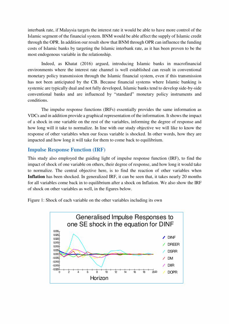
Impulse Response Function (IRF)
This study also employed the guiding light of impulse response function (IRF), to find the
impact of shock of one variable on others, their degree of response, and how long it would take
to normalize. The central objective here, is to find the reaction of other variables when
Inflation has been shocked. In generalized IRF, it can be seen that, it takes nearly 20 months
for all variables come back in to equilibrium after a shock on Inflation. We also show the IRF
of shock on other variables as well, in the figures below.
Figure 1: Shock of each variable on the other variables including its own
Generalised Impulse Responses toone SE shock in the equation for DINF
DINF
DREER
DSRR
DM
DIIR
DOPR
Horizon
-0.005
-0.010
-0.015
-0.020
0.000
0.005
0.010
0.015
0.020
0.025
0.030
0 2 4 6 8 10 12 14 16 18 2020
When inflation is shocked there is a response from all the variables and it takes at least 14 months for the rest of the variables to return to equilibrium.
The IRFs produce the same interpretation as VDC except that they are presented in a graphical
form.
Generalised Impulse Responses toone SE shock in the equation for DREER
DINF
DREER
DSRR
DM
DIIR
DOPR
Horizon
-0.005
-0.010
-0.015
-0.020
0.000
0.005
0.010
0.015
0 2 4 6 8 10 12 14 16 18 2020
Generalised Impulse Responses toone SE shock in the equation for DSRR
DINF
DREER
DSRR
DM
DIIR
DOPR
Horizon
-0.02
0.00
0.02
0.04
0.06
0.08
0.10
0 2 4 6 8 10 12 14 16 18 2020
Generalised Impulse Responses toone SE shock in the equation for DM
DINF
DREER
DSRR
DM
DIIR
DOPR
Horizon
-0.01
-0.02
0.00
0.01
0.02
0.03
0.04
0.05
0 2 4 6 8 10 12 14 16 18 2020
Generalised Impulse Responses toone SE shock in the equation for DIIR
DINF
DREER
DSRR
DM
DIIR
DOPR
Horizon
-0.005
-0.010
0.000
0.005
0.010
0.015
0.020
0.025
0.030
0 2 4 6 8 10 12 14 16 18 2020
Generalised Impulse Responses toone SE shock in the equation for DOPR
DINF
DREER
DSRR
DM
DIIR
DOPR
Horizon
-0.01
0.00
0.01
0.02
0.03
0.04
0.05
0.06
0 2 4 6 8 10 12 14 16 18 2020
Persistence Profile (PP)
Finally, employed the persistence profile analysis to indicate the general reaction and speed of
normalization to equilibrium in the event of an exogenous system-wide shock.
Figure 2: Persistence Profile
The application of the persistence profile analysis indicates that if the whole cointegrating
relationship is shocked, it will take about five periods (5 months) for the equilibrium to be
restored.
6. Conclusion
Our results show that there is a long term relationship between inflation, narrow money,
statutory reserve rate, real effective exchange rate and the Islamic interbank rate in the long
and short run. However we suggest that Inflation targeting may not be ideal in a dual banking
system. Alternatively, interest rate targeting is found to be most effective. Additionally, it will
give the central bank more control over the Islamic segment of the financial system.
Assessing monetary policy effectiveness in the presence of Islamic banking is complex, as it
requires examining it through multiple and sometimes conflicting dimensions. These include:
the fundamental Islamic principles of ex-ante interest payment prohibition and profit-and-risk
sharing; the spillovers from the conventional segment to the Islamic segment of the financial
system; and the monetary policy framework and instruments in place (Khatat, 2016).
Using interest rate targeting to have better control over the Islamic segment of the financial
system may not be accepted by all Islamic finance standard setters. However, there will be a
spillover from the conventional monetary policy transmission through the Islamic financial
system, even if this transmission has not been anticipated by the CB.
Persistence Profile of the effectof a system-wide shock to CV'(s)
CV1
Horizon
0.0
0.2
0.4
0.6
0.8
1.0
0 1 2 3 4 5 6 7 8 9 1010
Indeed as both segments of the financial system become more balanced, a unified monetary
policy stance might be feasible when there is arbitrage between the conventional and Islamic
segments of the financial system (Khatat, 2016).
Our results show that a unified monetary policy stance can be achieved by targeting the interest
rate and by using conventional and Islamic monetary policy instruments simultaneously.
Bibliography
Abdul Karim, Z., Said, F. F., Jusoh, M., & Thahir, M. Z. (2009). Monetary policy and inflation targeting in a small open-economy. Munich Personal RePEc Archive, Paper No. 23949.
Amadeo, K. ( 2016, October 17). What Is Inflation? How It's Measured and Managed. Retrieved from The Balance: https://www.thebalance.com/what-is-inflation-how-it-s-measured-and-managed-3306170
Bacha, O. I. (2008). The Islamic Inter bank Money Market and a Dual Banking System : The Malaysian Experience. Munich Personal RePEc Archive.
Bernanke, B. S., Woodford, & Michael. (1997). Inflation Forecasts and Monetary Policy. Journal of
Money, Credit and Banking, 29(4), 653-84.
BNM. (2016). ABOUT THE BANK. Retrieved from BNM: http://www.bnm.gov.my/index.php?ch=en_about&pg=en_intro&lang=en
BNM. (2016). Islamic Banking and Takaful. Retrieved from Bank Negara Malaysia.
BNM. (2016). Statutory Reserve Requirement. Kuala Lumpur: BNM.
BNM. (2017). Islamic Interbank Money Market. Retrieved from Bank Negara Malaysia: http://iimm.bnm.gov.my/index.php?ch=4&pg=4&ac=22
Cheong, L. M. (2005). Globalisation and the operation of monetary policy in Malaysia. BIS.
CIMB. (2017). CIMB ISLAMIC. Retrieved from CIMB: http://www.cimbbank.com.my/content/dam/cimb-consumer/personal/Important-Notices/OPR_BLR_BFR_Info.pdf
CNB. (2017). What is the nominal and real exchange rate? Retrieved from Czech National Bank: https://www.cnb.cz/en/faq/what_is_the_nominal_and_real_exchange_rate.html
Costa, S. (2000). Monetary Conditions Index. Economic bulletin, 97-106.
Croce, E., & Khan, M. S. (2000). Monetary Regimes and Inflation Targeting. Finance and
Development/IMF, 37(3), 48 -51.
Ericsson, N. R., Jansen, E. S., Kerbeshian, N. A., Nymoen, Ragnar, & and. (1998). Interpreting a Monetary Conditions Index. Bank for International Settlements.
Faiza Abbasi, K. R. (2016). CO2 emissions and financial development in an emerging economy: An augmented VAR approach. Energy Policy, 102–114.
Goodfriend, M., & King, R. (1997). The New Neoclassical Synthesis and the Role of Monetary. MIT
Press, 231 - 296.
Hill, H., Yean, T. S., & and Zin, R. H. (2012). Middle, Malaysia's Development Challenges: Graduating
from the Middle. Oxon: Routledge.
Investment&Finance. (2015, May 03). Islamic Alternatives to LIBOR. Retrieved from Investment&Finance: http://financialencyclopedia.net/islamic-finance/tutorials/islamic-alternatives-to-libor.html
Investopedia. (2017). Narrow Money. Retrieved from Investopedia: http://www.investopedia.com/terms/n/narrowmoney.asp
Jahan, S., & Mahmud, A. S. (2013). What Is the Output Gap? IMF FINANCE & DEVELOPMENT, Vol. 50, No. 3. Retrieved from http://www.imf.org/external/pubs/ft/fandd/2013/09/basics.htm
Khatat, M. E. (2016). Monetary Policy in the presence of Islamic Banks. International Monetary Fund.
Mishkin, F. S. (2004). Can Inflation Targeting Work in Developing Countries? National Bureau of
Economic Research.
Moyi, J. K. (2013). Monetary Conditions Index for Kenya . Research in Applied Economics, 1948-5433.
Muhamed Zulkhibri, R. S. (2016). Financing Channels and Monetary Policy in a Dual Banking System: Evidence from Islamic Banks in Indonesia. Review of Banking, FInancing and Monetary
Economics, 117-143.
Nicoletta Batini, K. T. (2000). Monetary Conditions Indices for the UK: A Survey. External MPC Unit, Discussion Paper No. 1.
Pei-Than Gan, K.-T. K. (2007). Estimating the Monetary Policy Rules for Malaysia: an optimal monetary conditions index. Economics Bulletin, 28(11), p.A1.
Pejman Abedifar, I. H. (2014). Finance-Growth Nexus and Dual Banking. hal, 01065676.
Pesaran, M., Shin, Y., & Smith, R. (2001). Bounds Testing approaches to the analysis of level relationships. Journal of Applied Economics, 289–326.
Poon, W.-C., & Tong, G.-K. (2009). The feasibility of inflation targeting in Malaysia. Economics
Bulletin, 29(2), 1035 -1045.
Ramkishen S. Rajan, R. S. (2003). Examining the Case for Reserve Pooling in East Asia: Empirical Analysis . IPS WORKING PAPERS.
Siklos, P. (2000). Is the MCI a Useful Signal of Monetary Policy Conditions? An Empirical Investigation. International Finance, 413-437.
Smets, F. (1997 ). FINANCIAL ASSET PRICES AND MONETARY POLICY:. BIS, No. 47.
Svensson, L. E. (2010). Inflation Targeting. CEPR and NBER.
Tor Jacobson, P. J. (1999). A VAR Model for Monetary Policy Analysis in a Small Open Economy. Working Paper Series, No 77.
Wu, T. Y. (2004). Does Inflation Targeting Reduce Inflation An Analysis for the OECD Industrial Countries. Banco Central Do Brasil, 1-26 .
Zulkhibri, A. M. (2010). Measuring Monetary Conditions in A Small Open Economy: The Case of Malaysia. IDB.