Is R&D Mispriced or Properly Risk-Adjusted?raw.rutgers.edu/docs/intangibles/Papers/Is...

Is R&D Mispriced or Properly Risk-Adjusted?

Mustafa Ciftci+, Baruch Lev

*, Suresh Radhakrishnan

**,

September 2009

+

State University of New York, Binghamton, NY, 13902 *Stern School of Business, New York University, New York 10012

**School of Management, University of Texas at Dallas, Richardson, TX 75080

Is R&D Mispriced or Properly Risk-Adjusted?

Abstract

Research has established that R&D-intensive firms are characterized by substantial future

risk-adjusted stock returns. The reasons for this phenomenon and its policy implications,

however, are widely debated. Some attribute the excess returns to investors‘ systematic

undervaluation of R&D firms and argue for improved disclosure to mitigate the mispricing,

while others claim that the excess returns are just compensating for an R&D-specific risk factor

and, therefore, no accounting changes are called for.

We aim at providing insights into this controversy by examining R&D firms with

substantial R&D outlays, i.e., firms with R&D as an important ingredient in their strategy.

Among such firms we compare firms with high and low industry-adjusted R&D intensity. The

high industry-adjusted R&D intensity firms are more likely to be engaged in basic research

activities, while the low industry-adjusted R&D intensity firms are likely to mimic and extend

existing technologies. As such, compared to the low industry-adjusted R&D intensity firms, the

high industry-adjusted R&D intensity firms are likely to suffer from higher information

asymmetry. We find that high industry-adjusted R&D intensity firms exhibit substantially

positive risk-adjusted returns during the first four-five future years, after which these excess

returns converge to those of low industry-adjusted R&D intensity firms. This evidence is

consistent with a significant undervaluation of high industry-adjusted R&D intensity firms. The

long-term excess returns are positive for both the high and the low industry-adjusted R&D

intensity firms and these excess returns are partly attributable to information risk. We also show

that the future excess returns of high industry-adjusted R&D intensity firms are substantially

lower for those firms who provide voluntary disclosure (earnings guidance) suggesting that the

short-term undervaluation is likely due to mispricing.

1

I. Introduction

We examine whether the widely-documented positive association of R&D spending with

future excess stock returns is due to investors‘ mispricing or to researchers‘ inadequate

adjustment for risk, and in the case of the latter, whether the future excess returns are attributed

to information risk, in which case there are important policy implications to draw. Lev and

Sougiannis (1996), Chan et al. (2001), Eberhart et al. (2004), Lev et al. (2005), and Lev et al.

(2007), among others, document that R&D outlays and their changes are positively associated

with future excess returns, suggesting that investors underreact to R&D outlays and that this

underreaction is partly attributable to the conservative accounting treatment of R&D spending. In

contrast, Chambers et al. (2002) argue that R&D‘s future excess returns are positive over the

long-term (ten years), suggesting that these returns are primarily attributable to risk. The R&D

risk-or-mispricing controversy has important implications for the state of capital market

efficiency, for practicable portfolio management (mispricing can be exploited by arbitrage), and

particularly for accounting standard-setting. For example, Skinner, in an opinion piece (2008),

rejects calls for increased disclosure about intangible investments and R&D by claiming that the

subsequent excess returns to R&D are attributable to inadequate adjustment for risk. Others beg

to differ. It is, therefore, of considerable importance to provide insights into the risk-or-

mispricing question of R&D.

While prior studies argue that mispricing or delayed reaction by investors to R&D

outlays is likely due to inadequate information on cash flows or biased assessment of R&D

prospects by investors (the numerator effect of stock valuation), there are no studies investigating

potential reasons for a higher risk of R&D firms (the denominator effect of valuation). The

literature on cost of capital or systematic risk identifies two important determinants of risk:

2

business risk and information risk.1 Applying this dichotomy to the ―source‖ of R&D risk—

business or information—is important because the two sources have different policy

implications. If business risk is the reason investors demand a higher return for R&D firms, then

fiscal incentives (R&D subsidies) are likely to mitigate R&D risk.2 On the other hand, if

information risk is the reason for investors‘ demand for a higher rate of return for R&D firms,

then standard-setting institutions can help mitigate such information risk through improved

disclosures. Thus, providing insight into the source of R&D risk is important for policy issues, as

is resolving the mispricing issue.

To address both the R&D mispricing-or-risk questions, and, if risk, whether business or

information risk, we examine a large sample of firms with substantial R&D outlays so as to

examine firms with R&D as an important strategy. Among such firms, and in contrast with

previous research on R&D which implicitly considered firms‘ R&D programs identical, we

strive to distinguish among R&D programs, since both investors‘ perceptions of R&D prospects

and the risk of R&D likely vary with the nature of R&D. Distinguishing among firms‘ R&D is

seriously hampered, though, because most firms don‘t provide any information about the nature

of R&D (e.g., how much research vs. development, basic vs. applied R&D, or the stage of

product development) beyond the total periodic outlays. We use the industry-adjusted R&D

intensity to distinguish between the nature of R&D activities. While the measure is based on

R&D intensity, adjusting for industry helps to distinguish between firms that are likely engaged

in basic versus applied research. For instance, the R&D intensity of generic drug manufacturers‘

in the pharmaceutical industry is higher than the R&D intensity of firms that engage in basic

1 See Beaver et al. (1970) and Kothari et al. (2002) for arguments that business risk likely affects the valuation of

R&D firms. Easley and O‘Hara (2004), Lambert et al. (2007), and Francis et al. (2005) show that information risk is

priced as an undiversifiable risk factor. 2 Firms also employ mechanisms such as R&D alliances and joint ventures to mitigate R&D risk.

3

research in the food products industry. Thus, R&D intensity by itself is not likely to discriminate

among the nature of R&D. Adjusting for R&D intensity within an industry group is consistent

with the arguments in the innovation and strategy literatures. Specifically, some firms use R&D

as a strategic tool for innovation; these firms strategically choose to be innovators and develop

new generations of products and services are likely to be the high industry-adjusted R&D

intensity firms. The low industry-adjusted R&D intensity firms mimic the products or services of

innovation high industry-adjusted R&D intensity firms and are low cost providers (see Porter

(1980)). Thus, within their industry high innovation firms are likely to have substantially higher

R&D levels than low innovation firms and their R&D is likely to be riskier (more research than

development) than low industry-adjusted R&D intensity firms‘ R&D.

We define the first five years after a firm is classified as high or low industry-adjusted

R&D within their industry as the short-term and the next five years as the long-term. We find

that high industry-adjusted R&D intensity firms‘ average short-term excess returns is roughly

five percent greater than that of low industry-adjusted R&D intensity firms. The long-term

excess returns of both high and low industry-adjusted R&D intensity firms are identical at

roughly 2.50% percent annually. This pattern of convergence of the excess returns of high

industry-adjusted R&D intensity firms from 5% in the first five years to 2.50% subsequently,

indicates mispricing. This return reversal of high industry-adjusted R&D intensity firms is

documented here for the first time.

We then examine the association between short-term and long-term R&D excess returns

and business and information risk proxies, controlling for other factors of risk examined in

earlier studies. We measure business risk by the standard deviation of future earnings and the

standard deviation of future cash flows, and information risk by the absolute value of analyst‘

4

earnings forecast errors, the dispersion of analysts‘ earnings forecasts, following Leuz (2003),

Heflin et al. (2003), and Bowen et al. (2002) as well as accruals quality, following Dechow and

Dichev (2002). We find that both business risk and information risk are positively associated

with both the short- and long-term excess returns, suggesting that the proxies of risk capture

additional priced risk factors. In addition, we find that high industry-adjusted R&D intensity

firms have roughly 2% greater short-term excess returns than low industry-adjusted R&D

intensity firms after controlling for business and information risk, indicating that this return is

likely attributable to mispricing. We also find that both high and low industry-adjusted R&D

intensity firms have no long-run excess returns after controlling for the proxies of business and

information risks. This indicates that the long-run excess returns are in part attributable to

information risk.

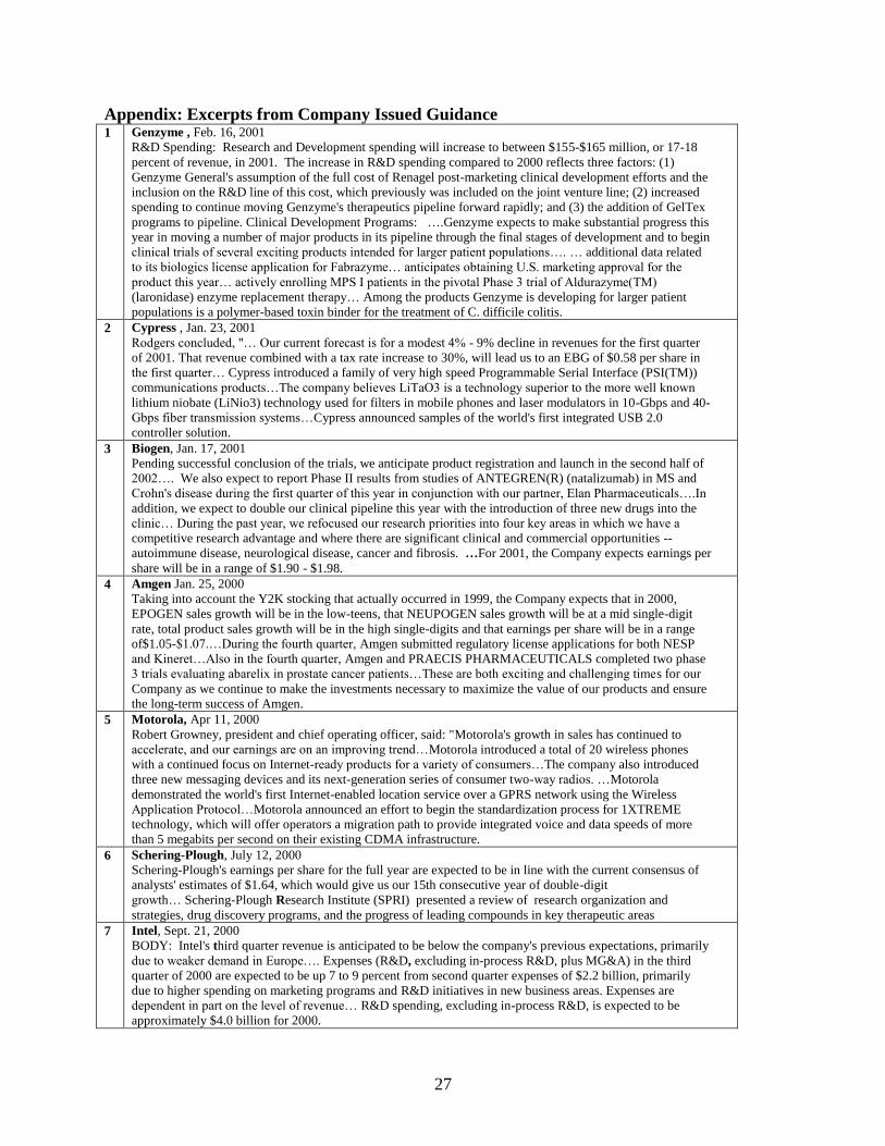
Finally, under the maintained assumption that firms that provide more earnings guidance

are also likely to provide more information to investors (see Jones, 2007), for a sub-sample of

firms with earnings guidance, we find that the short-term excess returns are substantially lower

for high industry-adjusted R&D intensity firms who provide more earnings guidance than for

high industry-adjusted R&D intensity firms who provide less guidance. This evidence suggests

that information asymmetry likely drives the short-term mispricing, and improved disclosure can

mitigate it.

The rest of the paper is organized as follows: Section II presents underlying rationale for

categorizing firms as high industry-adjusted R&D intensity firms and low industry-adjusted

R&D intensity firms, while Section III discusses the sample and the characteristics of high

industry-adjusted R&D intensity firms and low industry-adjusted R&D intensity firms. Section

5

IV provides the main empirical analysis; and Section V provides evidence of mispricing

mitigation by disclosure, and section VI concludes the paper.

II. Background on nature of R&D activities

This section discusses the importance of considering the nature of R&D activities. The

strategy literature suggests that based on core competence, competition and market structure,

firms strategically choose to be innovators by developing new generations of products, or

services, while other firms strategically choose to mimic the innovators and make the new

generation technology available to the masses (see Porter (1980)).3 As such, the nature of R&D

is likely to be substantially different for the innovators and mimicking firms. For example,

innovators will invest heavily in basic research in the development of new technologies, whereas

mimickers such as generic drug companies mainly focus on modifying current technologies.

Basic research is both more costly and risky than ―development‖ (modifying available

technologies). It stands to reason that the riskier basic research is more obscure from investors

than research on existing technology, and therefore will be associated with larger future excess

returns (mispricing)—our focus of analysis.

As a first step in distinguishing the different nature of R&D across firms, we use the

industry-adjusted R&D capital- to-sales ratio to classify high and low industry-adjusted R&D

intensity firms.4 There are two reasons for using an industry benchmark: First, the industry-

3 R&D programs reflecting innovation strategy can be classified on three-dimensions: the type of innovation that a

firm seeks to develop (product or process, see Cohen et al. (2000)), the nature/type of R&D activity (basic and

applied research activity or mainly development activity, see Griliches (1986) and Nelson and Romer (1996)), and

the coalitions and collaborations with other firms (outward- or inward-oriented strategy, see Baumol (2002)). There

is no requirement for firms to disclose this information and firms rarely voluntary disclose such information (Lev,

2001). 4 While data on patents is available and can be considered as a proxy for high industry-adjusted R&D intensity firms

and low industry-adjusted R&D intensity firms, Griliches (1986) provides reasons for why counting patents is not

adequate to distinguish between high industry-adjusted R&D intensity firms and low industry-adjusted R&D

intensity firms. Research that examines why firms patent only some innovations shows that (a) firms patent

6

adjusted R&D intensity controls for the competitive forces in the industry. For instance, even a

low industry-adjusted R&D intensity in the pharmaceutical industry will have a higher R&D

intensity than that of a high industry-adjusted R&D intensity in the food products industry. Using

the industry benchmark controls for the inter-industry differences in R&D intensity. Second,

Inklaar et al. (2004) state that items included in research and development spending vary widely

across industries. For instance, engineering firms include quality control costs in R&D

expenditures, while pharmaceutical firms do not include such costs. On the other hand,

pharmaceutical firms classify after market studies as R&D expenditures. Using the industry

benchmark controls for the differences across industries in the definition of R&D items.

Before proceeding with the stock market valuation of high and low industry-adjusted

R&D intensity firms, we validate in the next section that our classification of R&D firms to high

and low industry-adjusted R&D intensity firms captures fundamental attributes of risk and

returns of R&D firms.5

III. Characteristics of high and low industry-adjusted R&D intensity

We consider all firms with positive R&D expenditures from 1975 through 1997, having

financial information in the Compustat annual database.6 We delete firms with either sales less

than $10 million or total assets less than $5 million to exclude negligible firms. We obtain data

innovations when infringement is easier to detect and prove, and (b) firms do not patent innovations that are difficult

to imitate (see Arundel and Kabla (1998), Brouwer and Klienknecht (1999)). 5 Our measure of high and low industry-adjusted R&D is similar in spirit to R&D leaders and followers alluded to in

the strategy and economics literature. In general, this stream of literature shows that R&D leaders have higher

profitability than R&D followers. Caves and Ghemawat (1992) use a small sample of firms and show that

innovators have higher profits than low industry-adjusted R&D intensity firms. Also see Caves and Porter (1977),

Gruber (1992), Klette (1996) and Cardinal and Opler (1995). Consistent with these findings, in unreported analysis,

we find that high industry-adjusted R&D intensity firms have higher future profitability as measured by return on

assets and return on equity than low industry-adjusted R&D intensity firms. Also, the strategy literature emphasizes

that firms self-select to either being a leader or a follower, based on their core-competence/capabilities. We assume

that firms make this choice in an appropriate fashion. We do not explicitly control for such self-selection in our

research design, because we wish to examine the risk and return profiles of these groups. 6 The sample period extends up until 1997 because we examine long-term returns (six- to ten-years ahead returns).

Thus, for the returns we use data up until 2006. We check the robustness of our results by extending the sample to

2002 and find similar results.

7

on R&D expenditures (Compustat data item # 46) and sales (Compustat data item # 12) from the

Compustat annual database, and data on stock prices and number of shares outstanding from the

CRSP database. We obtain analysts‘ earnings forecasts and forecast dispersion from IBES

Summary Files, and require that firms are followed by at least two analysts so that the measure

of forecast dispersion is a meaningful proxy of information risk.

Following Chambers et al. (2002), we use the R&D capital-to-sales ratio to indicate R&D

intensity. The benchmark R&D intensity of the industry is the weighted average R&D capital–

to–sales of all firms in the industry group, where the weights are sales. For the industry groups,

we use the 48 industries in Fama and French (1997).7 We use the weighted industry average to

minimize the influence of small firms spending a large proportion of their revenues on R&D and

skewing the classification.8 Firms whose R&D intensity is greater than the benchmark R&D

intensity for the industry are classified as high industry-adjusted R&D intensity firms, and the

rest as low industry-adjusted R&D intensity firms.

Table 1, Panel A provides several characteristics of high and low industry-adjusted R&D

intensity firms. Out of the annual average of 399 firms, 253 firms or 63% are classified as high

industry-adjusted R&D intensity firms. There are fewer low industry-adjusted R&D intensity

firms than high industry-adjusted R&D intensity firms because we consider only the top three

quintiles of R&D capital-to-sales firms, to eliminate from the sample firms with negligible R&D

activities and we use value-weighted industry benchmark. Panel B of Table 1 provides evidence

on the persistence of the high and low groups: 59.49% (51.62%) of high (low) industry-adjusted

R&D intensity firms continue to be high (low) industry-adjusted R&D intensity firms after the

fifth year following classification, indicating that the classification is a long-term strategic choice

7The mapping is obtained from Ken French‘s website

http://mba.tuck.dartmouth.edu/pages/faculty/ken.french/data_library.html . 8 When we use equally-weighted industry average we obtain similar results.

http://mba.tuck.dartmouth.edu/pages/faculty/ken.french/data_library.html

8

by the firm. After five years, low R&D intensity firms are more likely to become high R&D

intensity firms than vice versa.

Both high and low industry-adjusted R&D intensity firms exhibit similar survival rates:

28.58% (26.03%) of high (low) industry-adjusted R&D intensity firms leave our sample after

five years. Panel C of Table 1 provides the reasons for firms not in our sample after five years.

For this purpose, we use the delisting codes as in Shumway (1997). Roughly 80% of both the

high and the low groups are not-in-sample after five years due to mergers and acquisitions; and,

12%-13% of the both the high and low groups are not-in-sample due to performance-based

listing requirement violations. That is, firms that are not-in-sample due to poor performance is

roughly 3% [=28% × 13%] for both the high and low R&D groups.

Panel D provides descriptive statistics for some firm characteristics of the high and low

groups. The panel reports the mean value of annual mean, and the t-statistics are computed using

the standard errors of the annual mean (see Fama and MacBeth (1973)). The mean R&D capital-

to-market value for high (low) industry-adjusted R&D intensity firms is 25.18% (14.64%),

suggesting that low industry-adjusted R&D intensity firms are considerably less R&D-intensive

than high industry-adjusted R&D intensity firms. The book-to-market ratio and dividend yields

of the high group are lower than that of low group, however, only the difference in book-to-

market is marginally significant. The mean sales growth is higher for the high than the low

group. In addition, the market share for high group is marginally greater than that for low group.

The high industry-adjusted R&D intensity firms are larger companies, as indicated by the mean

book value of equity, total assets and sales. However, they are more profitable, as indicated by

the return-on-assets, (return on asset is computed using operating income before R&D spending

to focus on operational difference across high industry-adjusted R&D intensity firms and low

9

industry-adjusted R&D intensity firms). All descriptive statistics indicate the existence of

fundamental operating differences between high and low industry-adjusted R&D intensity firms.

Kothari et al. (2002) find that R&D expenditure is more strongly associated with the

standard deviation of future earnings than capital expenditures. This suggests that R&D

expenditures increase business risk. Our research objective is to examine whether systematic

differences in the relationship between R&D and business risk exist for high and low industry-

adjusted R&D intensity firms. We thus augment the Kothari et al. (2002) model and estimate the

following equation:

SDi, t =[Industry Fixed Effects]+ β1t IRDHi, t + 2t R&DMi, t + 2t IRDHi, t*R&DMi, t

+ 3t CapExi, t + 4t LMVi, t + 5tLEVi, t + errort, (1)

where SD is the standard deviation of earnings-per-share before extraordinary items and

discontinued operations (Compustat data item # 58), and alternatively, the standard deviation of

cash flow from operations (Compustat data item # 308).9 The standard deviation is calculated

using five annual earnings/cash flow observations for years t+1 through t+5, and each earnings

observation is deflated by the stock price, P, at the beginning of the period t.10

The indicator

variable IRDH is one if a firm has a positive (zero for negative) industry-adjusted R&D Capital–

to–Sales in year t. The industry-adjusted R&D capital-to-sales is R&D capital-to-sales for a

given firm minus the industry‘s sales-weighted R&D capital–to–sales. The variable R&DM is

the R&D expenditure per share deflated by P.11

CapEx is the capital expenditure per share

(Compustat data item # 128) deflated by P. LMV is the natural logarithm of the market value of

9 Cash flow from operations is based on the statement of cash flows for 1987 to 1997. For 1975-1986, similar to

Givoly and Hayn (2000), cash flow from operations = fund from operations – (∆ current assets + ∆ debt in current

liabilities – ∆ current liabilities – ∆ cash). 10

Similar to Kothari et al. (2002) when earnings or cash flow data are missing for any year t+1 through t+5, the

standard deviation is set equal to the mean of SD for the firms in the same Altman Z-Score decile portfolio in year t. 11

While our test variable is based on R&D Capital to Sales, we use R&DM for the R&D exposure so as to be

consistent with Kothari et al. (2002). The coefficient estimate on R&DM is qualitatively similar to that obtained by

Kothari et al. (2002). In unreported analysis using R&D Capital to Sales instead of R&DM the R&D Capital to Sales

is not statistically significant, but IRDH and its interaction with R&D Capital to sales are qualitatively similar.

10

equity in April. LEV is the ratio of book value of debt (Compustat data item # 9 plus Compustat

data item # 34) to the market value of equity plus debt.

The coefficient estimate, β1 in equation (1) captures the abnormal standard deviation of

future earnings/cash flows for the high industry-adjusted R&D intensity firms compared to the

low industry-adjusted R&D intensity firms, and the coefficient estimate, β12 captures the

additional standard deviation of high industry-adjusted R&D intensity firms‘ earnings and cash

flows compared to that of low industry-adjusted R&D intensity firms for a dollar of R&D, after

controlling for other factors, such as size, financial and operating leverage, and industry effects.

Table 2, Panel A provides descriptive statistics of the variables used to estimate equation

(1). The average standard deviation of earnings (cash flows) for the high group is greater (lesser)

than that of the low group: the mean standard deviation of earnings (cash flows) of high and low

industry-adjusted R&D intensity firms are 0.0319 and 0.0321 (0.0293 and 0.0345), respectively.

However, only the difference in standard deviation of earnings is marginally significant. While

the marginally higher variability of the high group is consistent with Kothari et al. (2002), we

note that the low group have significantly higher capital expenditures and larger financial

leverage than the high group, and these variables are positively associated with the variability of

earnings (see Kothari et al. (2002)). The higher capital expenditure for the low group is

consistent with the notion that firms choose their strategy appropriately: firms with intangible

core competency such as research and development are likely to use less of the brick and mortar,

tangible assets. The higher capital expenditure is consistent with higher financial leverage for the

low group, as well as the notion that intangible assets are not financed through debt.12

Most

importantly, we need to control for these differences as in equation (1), before drawing

conclusions on the relationship between business risk and nature of R&D.

12

The mean LMV is negative because the market value of equity is in billions of dollars (see Kothari et al., 2002).

11

Table 2, Panel B provides the results of estimating equation (1). We find that the standard

deviation of the high group is lower than that of the low group for a dollar of R&D: β12 = -

0.0388, when the dependent variable is the standard deviation of earnings, and β12 = -0.0623

when the dependent variable is the standard deviation of cash flow from operations. These

differences are statistically significant, and indicate that high industry-adjusted R&D intensity

firms have lower business risk than low industry-adjusted R&D intensity firms for a dollar of

R&D spending.13

This counterintuitive finding is explained in the economics and strategy literature which

argues that innovators typically engage in multiple research projects (see Szwejczewski et al.

(2006), Eilat (2006)), which provide them with a greater opportunity to diversify the business

risk across these projects. Innovators are also likely to diversify the higher business risk of

individual research projects through joint ventures, alliances and consortiums (Naomi, 1989).

Furthermore, innovators not only engage in their own development activity but also license their

innovation and earn revenues (see Lev (2001)). This enables them to mitigate their risk exposure

even if a research project does not result in commercial development on their own. Also, the

barrier to entry created through innovation decreases dissolution risk (Banbury and Mitchell

(1995)). Thus, our finding is consistent with the notion that innovators, i.e., high industry-

adjusted R&D intensity firms are likely to mitigate the risk of research projects by (a) holding

more diversified research portfolios, (b) having additional options with successful research, (c)

13

We estimate equation (1) without the interaction between high industry-adjusted R&D intensity with R&DM and

find that the main effect, industry-adjusted R&D intensity is negative and significant, indicating that controlling for

other factors high industry-adjusted R&D intensity firms have a lower business risk than low industry-adjusted R&D

intensity firms. In unreported analysis we also find that both the high industry-adjusted R&D intensity firms and low

industry-adjusted R&D intensity firms have lower standard deviation of earnings and cash flows than the first two

quintiles of R&D firms.

12

diversifying more risky research thorough joint ventures and alliances, and (d) reducing

dissolution risk due to barriers to entry.

Moving to information risk, we use the absolute value of analysts‘ earnings forecast

errors and analysts‘ earnings forecast dispersion as proxies for information risk or its inverse—

information quality. Prior studies suggest that dispersion of analysts‘ forecasts reflects

information quality and the quality of the firms‘ disclosures (Lang and Lundholm (1996),

Krishnaswami and Subramaniam (1998), Luez (2003)). Similarly, Heflin et al. (2003) use

analysts‘ forecast errors and dispersion of analysts‘ forecast to examine the impact of Regulation

Fair Disclosure on the quality of information available to investors. In addition, we use the

accruals quality measure developed Dechow and Dichev (2002) as another proxy of information

risk. Francis et al. (2005) show that information risk as measured by accruals quality is a priced-

in risk factor. We augment Lang and Lundhom‘s (1996) model and estimate the following

equation.

IRi,t+1 = [Industry Fixed Effects]+ β1t IRDHi,t+2t R&DMi,t +2t IRDHi,t*R&DMi,t

+ 3t STDROEi,t +4t LMVi,t+5tCORRi, t + 6tACHEPSi,t+7t ROAi,t + t PROAi,t

+ errort,

(2)

where IRi, t+1 = {A_ERRORi, t+1, DISPi, t+1, WCAQ}. A_ERROR is analysts‘ forecast error

computed as the absolute value of the difference between actual earnings and median analysts‘

forecast scaled by the absolute value of the median analysts‘ forecast. DISP is the standard

deviation of analysts‘ earnings forecasts scaled by the absolute value of the median analysts‘

earnings forecast. Analyst forecast error and dispersion are measured in May following the fiscal

year and forecasts are obtained from IBES Summary Files. WCAQ is accrual quality computed

as the standard deviation of firm-specific residuals from the annual regression of working capital

accruals on cash flows in years t-1, t and t+1 for each industry group using data from year t to

year t-4 (see Francis et al. (2005), Dechow and Dichev (2002)). We use Fama and French (1997)

13

48 digit industry definitions in the estimation. Accrual quality indicates how well accruals map

into future cash flows. Francis et al. (2005) argue that to the extent the firm-specific residual is

consistently higher or lower, i.e., the standard deviation of firm-specific residuals is lower, the

accruals quality is better. They also find results consistent with the notion that lower accruals

quality is associated with higher cost of capital, i.e., is priced-in. STDROE is the standard

deviation of return on equity in the preceding five-years. Return on equity is earnings before

extraordinary items (data18) divided by book value of equity (Compustat data item # 60).

ACHEPS is the absolute value of change in earnings per share scaled by stock price. CORR is

the Pearson correlation coefficient between annual return and return on equity computed over the

preceding five years. ROA is the return on assets, computed as earnings before extraordinary

items divided by total assets (Compustat data item # 6). PROA is the average of past five years

earnings divided by the average of past five years total assets. All other variables are defined in

equation (1).

Table 3, Panel A provides the descriptive statistics of the variables used to estimate

equation (2). The one-year ahead absolute forecast error and forecast dispersion are substantially

higher for the high group. However, there is not a significant difference in accrual quality across

the high and low groups. The current and past performance of the high group as measured by

ROA and PROA is lower than that of the low group, possibly indicating the effect of

conservative accounting (R&D expensing).14

Table 3, Panel B provides the results of estimating equation (2). Both the absolute value

of forecast error and the forecast dispersion are higher for the high group than the low group: the

coefficients on IRDH (β1) are 0.0612 and 0.0412, respectively, and both are statistically

14

This may appear to be at odds with the discussion in Table 1, Panel C. The metric in Table 1, Panel C is the

operating earnings while the metric here is the bottom line earnings.

14

significant. The coefficients on the interaction term (β12) for absolute value of forecast error and

forecast dispersion are 2.3242 and 0.3548, respectively, and both are statistically significant.15

The results are qualitatively similar with accruals quality, WCAQ: the coefficient estimate on the

interaction term (β12) is 0.0928. Overall, the results are consistent with the information quality of

the high group being lower than that of the low group. Our findings suggest that the information

asymmetry between the firm and its investors is larger for high industry-adjusted R&D intensity

firms than low industry-adjusted R&D intensity firms. This is likely to occur because it may be

difficult if not impossible for investors to discern the nature and productivity of high industry-

adjusted R&D intensity firms‘ research efforts (basic research).16

Overall, these tests show that among the firms with substantial R&D outlays, the high

and low industry-adjusted R&D intensity firms are substantially different in their fundamental

risk characteristics. In particular, compared to the low industry-adjusted R&D firms, the

information (business) risk is higher (lower) for the high industry-adjusted R&D intensity firms.

We now turn to the main part of our analysis—the association of future excess returns of R&D

firms and risk.

IV. Excess returns of high and low industry-adjusted R&D intensity and their

causes We begin our main empirical analysis by tracking the high and low industry-adjusted

R&D intensity firms‘ excess stock returns for ten years subsequent to classification. Following

Chan et al. (2001), each firm in the sample is assigned to a companion portfolio based on size

and book-to-market, to compute excess returns. For the companion portfolio, firms are grouped

15

We also use the probability of information-based trading measure, PIN as in Easley et al. (2002). For this purpose,

we obtain data on PIN from Soeren Hvidkjaer‘s web site for the period of 1983 to 1997.We find that the PIN

measure is not different across the high and low groups, in both the univariate and multivariate analysis. Mohanram

and Rajagopal (2009) show that PIN is not a priced-in risk factor, and as such may not be capturing information risk. 16

FASB‘s Business Reporting Research Project‘s first steering committee‘s report shows that there was a lack of

meaningful and useful disclosures about intangible assets. The link for the report:

http://www.fasb.org/brrp/BRRP2.PDF

15

by the book-to-market ratio into five equal groups at the end of April each year, and the size

breakpoints are determined by classifying the companies into five equal groups in April each

year. The group representing the smallest size is further divided into two equal groups. Thus, we

have five groups of book-to-market ratio and six groups of size to determine the companion

portfolio. The monthly excess returns are then computed as the difference between the firm‘s

monthly return and the companion portfolio‘s monthly return. The annual excess returns are

obtained by compounding the monthly excess returns from May to April of next year. Also,

based on Kothari et al. (2005), to avoid ―passive truncations,‖ we substitute the value-weighted

market portfolio returns corresponding to the companion portfolio for non-surviving firms.17

Similar to Chambers et al. (2002) we track the future excess returns for ten years. We

consider the first five years following the R&D intensity classification as the short-term and the

second five years as the long-term.

Short-term Future Excess Returns, Business Risk and Information Risk

To examine the relation between business risk and information risk on the one hand and

future excess returns on the other hand, after accounting for other known risk factors, we

augment Penman and Zhang‘s (2002) model and estimate the following equations.

ARETi, t+1, +5 = β0 + β1 IRDHi, t + β2 SDi(EPSt+1, +5) + β3 SDi(CFPSt+1, +5) + 4 AvERi, t+1, +5

+ 5 AvDISPi, t+1, +5 + 6 AvWCAQi, t+1, +5 + δ1 AvEPi, t+1,+5δ2 LBMi, t+δ3 LLEVi, t

+ δ4 LMVi, t + δ5 EP+i, t + δ6 EP_DUMi, t + δ7 LARGE_INCi, t + errort+1,t+5

(3)

where ARET is the average short-term size and book-to-market adjusted returns over (t+1) to

(t+5). AvERi,t+1,+5 is the average absolute analysts‘ median forecast error from year (t+1) to

(t+5), scaled by the absolute value of median forecast in (t+1). AvDISP is the average dispersion

17

Passive truncations refer to the non-survival bias in future excess returns. Kothari et al. (2005) show that passive

truncations bias future excess returns, either higher or lower depending on the size of the firm. Chambers et al.

(2002) find that the average excess returns are about 3.80% over years six to ten for high R&D firms, whereas it is

around 2.24% in our sample. When we drop the analyst following criteria (to be comparable to their sample), the

average excess returns are about 4.39 % over year six to ten in our sample, which is quite close to long-run returns

in Chambers et al. study.

16

of analysts‘ forecasts from year (t+1) to (t+5), scaled by the absolute value of median forecast in

(t+1). Analyst forecast variables are all measured in May and forecasts are obtained from IBES

Summary Files. AvWCAQ is average WCAQ, accrual quality from year (t+1) to (t+5). AvEP is

the average earnings over the average of earnings from year (t+1) to (t+5) divided by share price

at time t. EP(+) is the earnings-to-price ratio if EP is positive and zero otherwise. Earnings to

price ratio is earnings before extraordinary items (data18) divided by market value of equity.18

EP_DUM is one if the current earnings to price ratio is negative. LBM is the natural logarithm of

the book-to-market ratio. Book-to-market ratio is book value of equity (Compustat data item #

60) divided by market value of equity. LMV is the natural logarithm of the market value of

equity. LLEV is the natural logarithm of the ratio of book value of debt (Compustat data item # 9

plus Compustat data item # 34) to the market value of equity plus debt. LARGE_INC is an

indicator variable for large R&D increases. A large R&D increase is given by an increase of 5%

in the R&D to asset ratio as well as in the R&D expenditure, for firms with R&D to asset ratio of

at least 5%: that is, a firm with R&D to asset ratio in year t-1 of 5% should have an R&D to asset

ratio of at least 5.25% in year t to be considered a firm with large R&D increase (see Eberhart et

al. (2004).

In equation (3) the standard deviation of earnings and cash flows are proxies for business

risk, and the absolute value of analysts‘ forecast error, forecast dispersion and accrual quality are

proxies for information risk. We expect the coefficients β2 through β6 on proxies for business and

information risk to be positive. Of course, if business and information risks are captured by risk

factors such as book-to-market, size, earnings-to-price and leverage, then proxies for business

and information risk are not likely to be associated with future returns. However, Francis et al.‘s

18

The definition of earnings used here is different from operating income used in Table 1, and corresponds to

Penman and Zhang (2002).

17

(2005) result shows that information risk is a priced-in risk factor over and above the other risk

factors: as such, we expect that information risk is not completely accounted for by the control

variables alone.19

Our test variable is IRDH. The intercept estimate, β0 captures the future excess returns of

low industry-adjusted R&D intensity firms, and the coefficient estimate on high industry-

adjusted R&D intensity firms IRDH, β1 captures the additional future excess returns of high

industry-adjusted R&D intensity firms relative to low industry-adjusted R&D intensity firms. We

expect β0 and β1 to be positive based on the mispricing/delayed reaction in the short-term

documented by prior studies of mispricing (see Chan et al. (2001)). Of course, β1 is expected to

be zero if all of the short-term excess return is accounted for by business and information risk, as

well as the other risk factors.20

We include AvEP as a control variable to account for a potential correlated omitted

variable of contemporaneous earnings. The LARGE_INC is a control variable for shifts in

research and development spending. Eberhart et al. (2004) shows that the future performance of

LARGE_INC is higher than that of other firms. In our context, it is possible that a low group

firm migrates to the high group (see Table 1, Panel B) because of a large increase in R&D

expenditure. LARGE_INC controls for the possibility of such a correlated omitted variable

driving our results. All other control variables are risk factors that have been documented to be

associated with future returns (see Penman and Zhang (2002)).

19

Core et al. (2008) use a different research design and find that accruals quality is not priced-in 20

We do not consider the interaction between IRDH and the business and information risk proxies. The results

discussed in Tables 2 and 3 indicate that the interaction between IRDH and the R&D expenditure is associated with

business and information risks. Thus, including the business and information risk proxies, already accounts for the

interaction effect. In unreported analysis including an interaction between IRDH and business and information risk

proxies does not affect the results qualitatively. The interaction terms are not statistically significant.

18

Table 4, Panel A provides the descriptive statistics of the variables in equations (3) and

not already presented in earlier tables. The reported numbers are the mean of the annual means

and the t-statistics are computed using the standard errors of the annual mean (see Fama and

MacBeth (1973)). The abnormal return for the high (low) industry-adjusted R&D intensity firms

is 5.25% (2.49%): a difference of roughly 110% = [5.25 – 2.49/ 2.49]. It follows that the

difference is statistically significant. The earnings to price ratio (EP+) is lower for the high group

than low group, indicating that firms in the high group are growth companies. However, the

differences are not significant. The high group have a higher proportion of negative earnings

(EP_DUM).

Table 4, Panel B provides the results of estimating equation (3). The mean of the annual

coefficient estimates are reported, and the t-statistics are computed using the standard errors of

the annual mean estimates (Fama and MacBeth, 1973). The coefficient on the standard deviation

on earnings, SD(EPS), is positive and significant [β2 = 1.0234 with t=5.21] and the coefficient on

forecast dispersion, AvDISP is also positive and significant [β5 = 0.1761 with t=4.11]. Thus, both

information and business risks are associated with the short-term excess returns. Given that mean

SD(EPS) and AvDISP in Panel A for the high group is 0.0319 and 0.1931, the average effect of

SD(EPS) and AvDISP in returns are 3.27% and 3.40%: for SD(EPS) it is calculated as (0.0319 x

1.0241) and for dispersion (0.1931 x 0.1761). Thus, on average both information and business

risks are priced-in.

Controlling for information and business risks, we find that the coefficient estimate on

the high group is positive and statistically significant [β1 = 0.0234 with t=4.69]. The coefficient

on the high group without controlling for business and information risks is β1 = 0.0323 with

t=5.46. Comparing the coefficients on the high group with and without the controls for business

19

and information risk suggests that roughly 38% [=0.0323 – 0.0234/0.0234] of the high industry-

adjusted R&D intensity firms‘ short-term excess returns is attributable to business and

information risk. Importantly, this indicates that after controlling for information and business

risks, high industry-adjusted R&D intensity firms continue to earn excess returns in the short-

term, which is indicative of mispricing: The intercept estimate in Panel B is negative and

significant [β1 = -0.0201 with t=-2.58] after controlling for business and information risk.

Leverage, book-to-market and size are not significant, most likely because the excess

returns (dependent variable) are already book-to-market and size adjusted. Earnings-to-price

ratio is marginally significant, indicating that the book-to-market and size adjusted returns do not

completely account for the risk factor captured by the earnings-to-price ratio. The LARGE_INC

dummy is significant suggesting that after controlling for R&D intensity, R&D growth is

positively associated with returns.

Long-term Future Excess Returns, Business Risk and Information Risk

Similar to equation (3) we consider the long-term returns by estimating the following

equation.

ARETi, t+6, +10 = β0+β1 IRDHi, t + β2 SDi(EPSt+6, +10) + β3 SDi(CFPSt+6, +10) + 4 AvERi, t+6, +5

+ 5 AvDISPi, t+6, +5 + 6 AvWCAQi, t+1,+5 +δ1 AvEPi, t+6,+10+ δ2 LBMi, t + δ3 LLEVi, t

+ δ4 LMVi, t + δ5 EP+i, t + δ6 EP_DUMi, t + δ7 LARGE_INCi, t + errort+6, +10

(4)

where all variables are as defined in equation (3) with subscripts (t+6), (t+10) indicating the

years over which the variable is averaged or cumulated.

Similar to the equation (3), we expect the coefficients β2 through β6 on proxies for

business and information risk to be positive. Our test variable is IRDH. We expect β0 and β1 to be

zero if all of the long-term excess return is accounted for by business and information risk, as

well as the other risk factors. However, if β1 is positive then it is indicative of a potential omitted

risk factor.

20

Table 5, Panel A provides the descriptive statistics of the variables in equations (4) not

already presented in earlier tables. The reported numbers are the mean of the annual means and

the t-statistics are computed using the standard errors of the annual mean (see Fama and

MacBeth (1973)). The abnormal return for the high (low) industry-adjusted R&D intensity firms

is 2.54% (2.77%): a difference of roughly -8% = [2.54 – 2.77/ 2.77]. This is a substantial drop

from the 110% difference in the short-term (see Table 4, Panel A). The difference in the long-

term excess returns across the high and low groups is not statistically significant. This reversal

provides an indication of potential mispricing (we investigate this more in the next sub-section).

The difference in business risk across high and low groups is not statistically significant, but the

difference in information risk continues to be statistically significant as in the short-term.

Table 5, Panel B provides the results of estimating equation (4). The coefficient on the

standard deviation on earnings, SD(EPS), is positive and significant [β2 = 0.8641 with t=3.73]

and the coefficient on forecast dispersion is also positive and significant [β5 = 0.0905 with

t=2.72]. Thus, both information and business risks affect the long-term excess returns. Given that

mean SD(EPS) and AvDISP in Panel A for high group is 0.0291 and 0.1606, the average effect

of SD(EPS) and AvDISP in returns are 2.48% and 1.43%: for SD(EPS) it is calculated as

(0.0291 × 0.8547) and for dispersion (0.1606 × 0.0892). Thus, on average both information and

business risks are priced-in. Compared to the magnitudes of the average rate of return for

business and information risk for the short-term, the magnitudes are substantially lower for the

long-term. The degree of stability in the average rate of return for the short-term and long-term

suggests that the business and information risks are priced-in risk factors.

Controlling for information and business risks, we find that the coefficient on the high

group is not statistically significant [β1 = 0.0036 with t=0.54]. The intercept estimate is also

21

statistically not different from zero [β1 = -0.0199 with t=-1.19]. This indicates that after

controlling for information and business risks, high and low industry-adjusted R&D intensity

firms earn zero excess returns in the long-term. In unreported analysis, without including any

additional controls in equation (4) we obtain intercept and coefficient estimate on high industry-

adjusted R&D intensity firms similar to the long-term univariate average reported in Table 5,

Panel A. This indicates that information risk partly explains the long-term excess returns

documented in Chambers et al. (2002).

Comparison of Short- and Long-term Excess Returns

We focus on the time-series pattern of the excess returns for each group, since a major

characteristic of share mispricing is that investors learn over time, and ―correct‖ the mispricing at

some future date. Mispricing should therefore be reflected by reversal (or convergence) of excess

returns. Indeed, we see that high industry-adjusted R&D intensity firms‘ short- and long-term

returns are 5.25% (Table 4, Panel A) and 2.54% (Table 5, Panel A), respectively, indicating a

clear reversal of returns attributable to mispricing. 21

This return reversal is in stark contrast to Chamber et al. (2002). There are three potential

reasons for this: (a) difference in sample, (b) passive truncation adjustment, and (c) the

classification based on industry-adjustments. Chambers et al. consider the top three quintiles of

R&D capital intensity without the restriction of two analysts and show that the short-term returns

are similar in magnitude to the long-term returns. The top three quintiles correspond to our full

sample, because we examine only firms with substantial R&D outlays. In untabulated analysis,

21

For the whole group of high R&D firms, without separating high industry-adjusted R&D intensity firms and low

industry-adjusted R&D intensity firms, we find a similar reversal, although of lower magnitude. In particular, the

short- and long-term excess returns for high R&D firms are 5.40% and 2.24%, respectively. The magnitude of

reversal is 2.00% less than Table 4. Thus, the classification of high industry-adjusted R&D intensity firms and low

industry-adjusted R&D intensity firms using an industry benchmark helps to increase the short-term returns

considerably.

22

for our full sample which roughly corresponds to that of Chambers et al., without using the

passive truncation adjustment and restrictions on analyst following, we find that the short-term

excess returns is roughly 5.14% and the long-term excess returns is 4.39%, a substantial

reduction in the magnitude of the reversal.22

However, when we classify this sample into high

and low industry-adjusted R&D intensity firms, we find that the short- and long-term excess

returns for high industry-adjusted R&D intensity firms are 6.67% and 4.32%, respectively: a

significant reversal. This indicates the importance of the industry adjusted classification of R&D

intensity. Overall, sample differences do not drive the result of return reversal of high industry-

adjusted R&D intensity firms.

We also repeat our analysis using Chambers et al. (2002) procedure for computing future

excess returns for our sample of firms with at least two analyst following. The untabulated

results show that the short- and long-run excess returns for high industry-adjusted R&D intensity

firms are 8.04% and 5.00%. The magnitude of the reversal is 3.03% for high industry-adjusted

R&D intensity firms and is both economically and statistically significant. As such, the reversal

of high industry-adjusted R&D intensity firms‘ future excess returns is attributable to the

classification based on industry-adjustment which likely captures the differences in the nature of

R&D activity. 23

22

Chambers et al. substitute the companion portfolio return for non-surviving firms up until the end of the year of

non-survival. In subsequent years the non-surviving firms are excluded from the computation of excess returns. In

our passive truncation adjustment, we assume that the proceeds from the non-surviving firms are invested in value

weighted index portfolio. While non-survival leads to passive truncations, the non-survival of the high and low

groups are similar, and thus if the reversal is attributable to passive truncation alone, then we should observe

reversals for both the high and low groups. 23

In unreported analysis the results are qualitatively similar when either (a) the top two quintiles instead of top three

quintiles are considered, or (b) we do not make any adjustment for firms‘ non-survival, i.e., passive truncations. For

the bottom two quintiles not considered in our sample (a) the future excess returns are not statistically different from

zero, (b) the difference in excess returns across high industry-adjusted R&D intensity firms and low industry-

adjusted R&D intensity firms are not different from zero, and (c) the difference in excess returns across the short-

and long-terms are not different from zero.

23

The average annual return difference between high and low industry-adjusted R&D

intensity firms in the long-term is 0.08% which is statistically indistinguishable from zero. This

indicates that the high and low industry-adjusted R&D intensity firms‘ long-term excess returns

are identical. The equation (4) results in Table 5, Panel B indicates that accounting for risk

factors (including business and information risk), long-term excess returns of both high and low

industry-adjusted R&D intensity firms are statistically zero. As discussed earlier this reversal is

indicative of mispricing.

In summary, our analysis indicates: (1) During the first five years after classification,

high industry-adjusted R&D intensity firms are substantially undervalued by investors, after

accounting for both business and information risks, and various general risk factors embedded in

the size and book-to-market measures. (2) Beyond the first five years, the excess returns of high

and low industry-adjusted R&D intensity firms converge, and essentially reflect both business

and information risk factors. We note that these findings, indicating both an R&D undervaluation

of high industry-adjusted R&D intensity firms in the short-term, and the impact of information

risk on the entire series of subsequent returns of high industry-adjusted R&D intensity firms and

low industry-adjusted R&D intensity firms, is documented here for the first time. These findings

have, we believe, important policy implications, to be discussed in the concluding section.

V. Disclosure mitigates undervaluation

Empirical studies indicating undervaluation of R&D-intensive firms often attribute the

undervaluation of the deficient disclosure regarding R&D and related innovation activities (e.g.,

Eberhart et al., 2004). Such attribution and the logical policy implications—extended

disclosure—are frequently challenged with the argument that the researchers failed to show that

24

extended disclosure would mitigate the undervaluation (e.g., Skinner, 2008). A valid criticism

indeed.

To address this criticism and strengthen our policy recommendations we examine

whether extended disclosures by firms mitigate the R&D-related undervaluation. As an indicator

of extended disclosure we use the number of managements‘ earnings forecasts in a given year.

While managements‘ earnings forecasts are often short-term, we assume that firms that have a

communications strategy of providing short-term earnings guidance will also provide investors

with long-term forward-looking information.

Specifically, we conjecture that the future excess returns of high industry-adjusted R&D

intensity firms issuing more earnings guidance should be smaller than for those with fewer

earnings guidance, given that some of the information conveyed by the guidance is related to

R&D and its consequences. In the Appendix, we provide excerpts of a few companies‘ earnings

guidance to illustrate that the guidance indeed contains information on R&D activities. In

general, our perusal of several news releases of earnings guidance reveals that firms provide a

variety of information: some provide information on R&D spending, and others provide

information on new products that have been introduced, some provide information on the

product pipeline. This is consistent with the recent findings of Jones (2007), and lends support

for our conjecture.

The management forecast data is obtained from Thompson Financial First Call database

which is available after 1994. Thus, we consider a sample from 1994 to 2001. For the empirical

analysis in this section we consider all firms with R&D that appear in the First Call database.24

24

We only consider firms with earnings guidance because firms without earnings guidance may be providing

information to investors using other channels such as conference calls.

25

We estimate the following model to investigate the impact of guidance on the future excess

returns to high industry-adjusted R&D intensity firms.

ARETi, t+1,t+3=[Year Dummy]+β1IRDHi, t+β2LN_FORCSTi, t+ β2D LN_FORCSTi, t*IRDH i, t

+ β3 STD(EPS t+1, t+3) + β4 STD(CFPS t+1, t+3)+β5AvERi,t+1,t+3+β6 AvDISPi,t+1,t+3

+ β7AvEPi,t+1,t+3 + 8 AvWCAQi, t+1, t+3 + β9 LBMi, t + β10 LLEVi, t + β11 LMVi, t

+ β12 EP +i, t + β13 EP_DUMi, t + β14 LARGE_INCi, t+ errort+1,t+3

(5)

ARETi,t+1,t+3 is the average size and book-to-market adjusted returns over a three year period

after portfolio formation (from t+1 to t+3). IRDH is one if a firm has a positive industry-adjusted

R&D Capital–to–Sales in year t. LN_FORCST is log of the number of management forecast in

year t. Equation (5) is estimated using panel data, and therefore we use the Huber-White

procedure to correct for the standard errors (see Petersen (2005)). Based on our earlier results,

we expect β1 to be positive and based on the communications strategy conjecture we expect β2D

to be negative. We examine the average abnormal returns over subsequent three years because

using return over five years decreases the sample size and test power considerably.25

Table 6 presents the results of estimating equation (5). The coefficient estimate on IRDH

(β1) is 4.32% and the coefficient estimate on the interaction of IRDH and managements‘ earnings

forecasts term, (β2D) is -2.42%. This indicates that about half of the short-term excess return of

high industry-adjusted R&D intensity firms is mitigated by the earnings guidance release,

providing support for the conjecture that the short-term excess returns (share undervaluation) are

likely due to deficient information. This result is similar to the average short-term excess returns

for high industry-adjusted R&D intensity firms reported in Table 4, suggesting that the average

annual future excess returns in this sub-sample for the period 1994-2001 is similar to that in our

main sample for the period 1975-1997.

25

In unreported analysis we use the average excess returns over five years instead of three years and the interaction

term is significant at the ten percent level: the sample period for this analysis is 1994-1999.

26

VI. Discussion

We set out to provide insights into a long-standing conundrum: Are the widely-

documented subsequent excess returns to R&D-intensive firms due to share mispricing or risk?

To this, we add another important question: If risk causes, fully or partially those subsequent

excess returns, is it business and/or information risk? The importance of these questions mainly

derives from the fact that both share mispricing and information risk has obvious disclosure

policy implications.

Our battery of tests indicates: (a) The shares of high industry-adjusted R&D intensity

firms are systematically undervalued during five years following classification. (b) This share

undervaluation is cut by half when high industry-adjusted R&D intensity firms release earnings

guidance, frequently discussing R&D-related issues. (c) Information risk affects the short- and

long-term subsequent excess returns of both high and low industry-adjusted R&D intensity

firms.

Regarding accounting policy implications, we note that our study goes beyond previous

ones by documenting, not just conjecturing, that voluntary disclosure (earnings guidance) indeed

mitigates the R&D-related undervaluation. This lends empirical support to the frequent calls for

enhanced disclosure of R&D and other innovation activities of companies. Such disclosures

include fundamental breakdowns of R&D outlays (e.g., basic research vs. development), and

data on the consequences of R&D, such as ―innovation revenues‖ (the percentage of periodic

revenues from recently introduced products/services). Research on European companies, which

have to provide ―innovation revenue‖ data, shows that this measure is a powerful predictor of

future firm performance (Crepon et al., 1998). Our aim in this study is to foster discussion on

enhanced disclosure by innovative companies.

27

Appendix: Excerpts from Company Issued Guidance 1 Genzyme , Feb. 16, 2001

R&D Spending: Research and Development spending will increase to between $155-$165 million, or 17-18

percent of revenue, in 2001. The increase in R&D spending compared to 2000 reflects three factors: (1)

Genzyme General's assumption of the full cost of Renagel post-marketing clinical development efforts and the

inclusion on the R&D line of this cost, which previously was included on the joint venture line; (2) increased

spending to continue moving Genzyme's therapeutics pipeline forward rapidly; and (3) the addition of GelTex

programs to pipeline. Clinical Development Programs: ….Genzyme expects to make substantial progress this

year in moving a number of major products in its pipeline through the final stages of development and to begin

clinical trials of several exciting products intended for larger patient populations…. … additional data related

to its biologics license application for Fabrazyme… anticipates obtaining U.S. marketing approval for the

product this year… actively enrolling MPS I patients in the pivotal Phase 3 trial of Aldurazyme(TM)

(laronidase) enzyme replacement therapy… Among the products Genzyme is developing for larger patient

populations is a polymer-based toxin binder for the treatment of C. difficile colitis.

2 Cypress , Jan. 23, 2001

Rodgers concluded, "… Our current forecast is for a modest 4% - 9% decline in revenues for the first quarter

of 2001. That revenue combined with a tax rate increase to 30%, will lead us to an EBG of $0.58 per share in

the first quarter… Cypress introduced a family of very high speed Programmable Serial Interface (PSI(TM))

communications products…The company believes LiTaO3 is a technology superior to the more well known

lithium niobate (LiNio3) technology used for filters in mobile phones and laser modulators in 10-Gbps and 40-

Gbps fiber transmission systems…Cypress announced samples of the world's first integrated USB 2.0

controller solution.

3 Biogen, Jan. 17, 2001

Pending successful conclusion of the trials, we anticipate product registration and launch in the second half of

2002…. We also expect to report Phase II results from studies of ANTEGREN(R) (natalizumab) in MS and

Crohn's disease during the first quarter of this year in conjunction with our partner, Elan Pharmaceuticals….In

addition, we expect to double our clinical pipeline this year with the introduction of three new drugs into the

clinic… During the past year, we refocused our research priorities into four key areas in which we have a

competitive research advantage and where there are significant clinical and commercial opportunities --

autoimmune disease, neurological disease, cancer and fibrosis. …For 2001, the Company expects earnings per

share will be in a range of $1.90 - $1.98.

4 Amgen Jan. 25, 2000

Taking into account the Y2K stocking that actually occurred in 1999, the Company expects that in 2000,

EPOGEN sales growth will be in the low-teens, that NEUPOGEN sales growth will be at a mid single-digit

rate, total product sales growth will be in the high single-digits and that earnings per share will be in a range

of$1.05-$1.07.…During the fourth quarter, Amgen submitted regulatory license applications for both NESP

and Kineret…Also in the fourth quarter, Amgen and PRAECIS PHARMACEUTICALS completed two phase

3 trials evaluating abarelix in prostate cancer patients…These are both exciting and challenging times for our

Company as we continue to make the investments necessary to maximize the value of our products and ensure

the long-term success of Amgen.

5 Motorola, Apr 11, 2000

Robert Growney, president and chief operating officer, said: "Motorola's growth in sales has continued to

accelerate, and our earnings are on an improving trend…Motorola introduced a total of 20 wireless phones

with a continued focus on Internet-ready products for a variety of consumers…The company also introduced

three new messaging devices and its next-generation series of consumer two-way radios. …Motorola

demonstrated the world's first Internet-enabled location service over a GPRS network using the Wireless

Application Protocol…Motorola announced an effort to begin the standardization process for 1XTREME

technology, which will offer operators a migration path to provide integrated voice and data speeds of more

than 5 megabits per second on their existing CDMA infrastructure.

6 Schering-Plough, July 12, 2000

Schering-Plough's earnings per share for the full year are expected to be in line with the current consensus of

analysts' estimates of $1.64, which would give us our 15th consecutive year of double-digit

growth… Schering-Plough Research Institute (SPRI) presented a review of research organization and

strategies, drug discovery programs, and the progress of leading compounds in key therapeutic areas

7 Intel, Sept. 21, 2000

BODY: Intel's third quarter revenue is anticipated to be below the company's previous expectations, primarily

due to weaker demand in Europe…. Expenses (R&D, excluding in-process R&D, plus MG&A) in the third

quarter of 2000 are expected to be up 7 to 9 percent from second quarter expenses of $2.2 billion, primarily

due to higher spending on marketing programs and R&D initiatives in new business areas. Expenses are

dependent in part on the level of revenue… R&D spending, excluding in-process R&D, is expected to be

approximately $4.0 billion for 2000.

http://www.lexisnexis.com/us/lnacademic/search/XMLCrossLinkSearch.do?bct=A&risb=21_T4048091168&returnToId=20_T4048093021&csi=227171&A=0.9353820896016745&sourceCSI=000000&indexTerm=%23CC0001U7O%23&searchTerm=MOTOROLA&indexType=C

http://www.lexisnexis.com/us/lnacademic/search/XMLCrossLinkSearch.do?bct=A&risb=21_T4048091168&returnToId=20_T4048143749&csi=227171&A=0.5305533048527445&sourceCSI=000000&indexTerm=%23CC0001U7O%23&searchTerm=Motorola&indexType=C

http://www.lexisnexis.com/us/lnacademic/search/XMLCrossLinkSearch.do?bct=A&risb=21_T4048091168&returnToId=20_T4048093021&csi=227171&A=0.9353820896016745&sourceCSI=000000&indexTerm=%23CC0001U7O%23&searchTerm=Motorola%20&indexType=C




28

References

Arundel A., I. Kabla. 1998. ―What percentage of innovations is patented?‖ Research Policy, 27: 127-141.

Banbury, C.M., W. Mitchell. 1995. ―The effect of introducing important incremental innovations on

market share and business survival.‖ Strategic Management Journal, 16: 161-182.

Baumol W. J. 2002. The Free Market Innovation Machine, Princeton University Press, Princeton, NJ.

Beaver, W., P. Kettler, and M. Scholes. 1970. ―The association between market determined and

accounting determined risk measures.‖ The Accounting Review, 45: 654-682.

Bowen R. M., A. K. Davis, D. A. Matsumoto. 2002. ―Do conference calls affect analysts‘ forecasts?‖ The

Accounting Review, 77: 285-316.

Brouwer E., A. Klienknecht. 1999. ―Innovative output and the firm propensity to patent: An exploration

of the CIS microdata,‖ Research Policy, 28: 615-624.

Cardinal, L.B., T.C. Opler. 1995. ―Corporate diversification and innovative efficiency: An empirical

study.‖ Journal of Accounting and Economics, 19: 365-382.

Caves, R.E., M.E. Porter. 1977. ―From entry barriers to mobility barriers: conjectural decisions and

contrived deterrence to new competition.‖ Quarterly Journal of Economics, 91: 241-262.

Caves, B.E., P. Ghemawat. 1992. ―Identifying mobility barriers.‖ Strategic Management Journal, 13: 1-

12.

Chambers, D., R. Jennings, R.B. Thompson II. 2002. ―Excess returns to R&D-intensive firms.‖ Review of

Accounting Studies, 7:133-158.

Chan, L, J. Lakonishok, and T. Sougiannis. 2001. ―The stock market valuation of research and

development expenditures.‖ Journal of Finance, 56: 2431-2457.

Cohen, M.A., Eliashberg, J., T.H. Ho. 2000. ―An analysis of several new product performance metrics.‖

Manufacturing & Service Operations Management, 2:337-349.

Core, J.E. W.R. Guay, R. Verdi. 2008. ―Is accruals quality a priced risk factor?‖ Journal of Accounting

and Economics, 46:2-22.

Crepon, B., E. Duguet, J. Mairesse. 1998. ―Research, innovation, and productivity: An econometric

analysis at the firm level,‖ Working Paper 6696, National Bureau of Economic Resarch, Cambridge,

MA.

Dechow, P.M., I.D. Dichev. 2002. ―The quality of accruals and earnings: The role of accrual estimation

errors.‖ The Accounting Review, 77: 35-59.

Easley, A.C., S. Hvidkjaer, M. O‘Hara. 2002. ―Is information risk a determinant of asset returns?‖

Journal of Finance, 57:2185-2221.

Easley, A.C., M. O‘Hara. 2004. ―Information cost of Capital.‖ Journal of Finance, 59:1553-1594.

Eberhart, A.C., W.F. Maxwell, A.R. Siddique. 2004. ―An examination of long-term excess stock returns

and operating performance following R&D increases.‖ Journal of Finance, 59: 623-651.

Eilat H. 2006. ―Constructing and evaluating balanced portfolios of R&D projects with interactions: A

DEA based methodology,‖ European Journal of Operations Research, 1723): 1018-1034.

Fama, E.F., K.R. French. 1997. ―Industry costs of equity.‖ Journal of Financial Economics, 43: 153-194.

Fama, E. F., J. MacBeth. 1973 ―Risk, return and equilibrium: Empirical tests.‖ Journal of Political

Economy, 81: 607-636.

http://www.jstor.org/view/01432095/di007650/00p0137y/0?currentResult=01432095%2bdi007650%2b00p0137y%2b0%2c01%2b19950700%2b9995%2b80049299&searchID=cc99333c.10866599390&frame=noframe&sortOrder=SCORE&[email protected]/01cc99333c0050138af92&dpi=3&viewContent=Article&config=jstor

http://www.jstor.org/view/01432095/di007650/00p0137y/0?currentResult=01432095%2bdi007650%2b00p0137y%2b0%2c01%2b19950700%2b9995%2b80049299&searchID=cc99333c.10866599390&frame=noframe&sortOrder=SCORE&[email protected]/01cc99333c0050138af92&dpi=3&viewContent=Article&config=jstor

http://www.jstor.org/view/00014826/ap010183/01a00030/0?currentResult=00014826%2bap010183%2b01a00030%2b0%2c01%2b19701000%2b9993%2b80298999&searchID=cc993341.10866609310&frame=noframe&sortOrder=SCORE&[email protected]/01cc99333c0050138af92&dpi=3&viewContent=Article&config=jstor

http://www.jstor.org/view/00014826/ap010183/01a00030/0?currentResult=00014826%2bap010183%2b01a00030%2b0%2c01%2b19701000%2b9993%2b80298999&searchID=cc993341.10866609310&frame=noframe&sortOrder=SCORE&[email protected]/01cc99333c0050138af92&dpi=3&viewContent=Article&config=jstor

http://www.afajof.org/Pdf/forthcoming/MS1617-R3.pdf

http://www.afajof.org/Pdf/forthcoming/MS1617-R3.pdf

http://weblinks2.epnet.com/citation.asp?tb=1&_uh=btn+N+6C9C&_ug=sid+F9CDBBB1%2D7E84%2D4FE1%2D917A%2DF2F168934572%40sessionmgr2+dbs+buh+DFA9&_us=hd+False+or+Date+fh+False+ss+SO+sm+ES+sl+%2D1+dstb+ES+ri+KAAACB1D00028202+2FD8&_ua=bo+B%5F+shn+1+db+buhjnh+bt+ID++%22ARW%22+64AB&_uso=tg%5B2+%2D+tg%5B1+%2D+tg%5B0+%2D+db%5B0+%2Dbuh+hd+False+clv%5B0+%2D19970000%2D19970000+op%5B2+%2DAnd+op%5B1+%2DAnd+op%5B0+%2D+cli%5B0+%2DDT1+st%5B2+%2D+st%5B1+%2DFRENCH+st%5B0+%2DFAMA+BFDE&fn=1&rn=2

29

Francis, J., R. LaFond, P. Olsson, K. Schipper. 2005. ―The market pricing of accruals quality,‖ Journal of

Accounting and Economics, 39: 295-327.

Givoly, D., C. Hayn. 2000. ―The changing time-series properties of earnings, cash flows and accruals:

Has financial reporting become more conservative?‖ Journal of Accounting and Economics, 29:287-

309.

Griliches, Z. 1986. ―Productivity, R&D and basic research at the firm level in the 1970s.‖ The American

Economic Review, 76: 141-154.

Gruber, H. 1992. ―Persistence of High industry-adjusted R&D intensity firmship in product innovation,‖

Journal of Industrial Economics, 40: 359-376.

Heflin, F., K. R. Subramanyam, Y. Zhang. 2003. ―RFD and the financial information environment: early

evidence,‖ The Accounting Review, 78:1-38.

Inklaar R., R.H. McGuckin, B. van Ark, S.M. Dougherty. 2004. ―The structure of business R&D: Recent

trends and measurement implications,‖ Working Paper, The Conference Board.

Jones, D. A. 2007. ―Voluntary disclosure in R&D-intensive industries,‖ Contemporary Accounting

Research, 24: 489-522.

Klette, T.J. 1996. ―R&D, scope economies and plant performance.‖ RAND Journal of Economics, 27:

502-523.

Krishnaswami, S., V. Subramaniam. 1998. ―Information asymmetry, valuation, and the corporate spin-off

decision,‖ Journal of Financial Economics, 53: 1315-1336.

Kothari, S.P., T.E. Laguerre, J.A. Leone. 2002. ―Capitalization versus expensing: Evidence on the

uncertainty of future earnings from capital expenditures versus R&D outlays.‖ Review of Accounting

Studies, 7: 355-382.

Kothari, S.P., J.S. Sabino, T. Zach. 2005. ―Implications of survival and data trimming for tests of market

efficiency.‖ Journal of Accounting and Economics, 39: 129-152.

Lambert R., C. Leuz, C., R.E. Verrecchia. 2007. ―Accounting information, disclosure and the cost of

capital.‖ Journal of Accounting Research, 38: 385-420.

Lang, M., R. Lundholm. 1996. ―Corporate disclosure policy and analyst behavior,‖ The Accounting

Review, 71: 467-492.

Leuz, C. 2003. ―IAS versus U.S. GAAP: Information asymmetry-based evidence from Germany‘s new

market,‖ Journal of Accounting Research, 41: 445-472.

Lev B. 2001. Intangibles: Management, Measurement and Reporting, Brookings Institution Press,

Washington D.C.

Lev, B., T. Sougiannis. 1996. ―The capitalization, amortization and value-relevance of R&D.‖ Journal of

Accounting and Economics, 21: 107-138.

Lev, B., B. Sarath, T. Sougiannis. 2005. ―R&D-related reporting biases and their consequences.‖

Contemporary Accounting Research, 22: 977-1026.

Lev, B., D. Nissim, J. Thomas. 2007. ―On the informational usefulness of R&D capitalization and

amortization,‖ in Visualizing Intangibles: Measuring and Reporting in the Knowledge Economy eds.

S. Zambon and G. Marzo, Ashgate Publishing Co.: 97-128.

Mohanram, P. S. Rajgopal. ―2009. ―Is PIN priced risk?‖ Journal of Accounting and Economics, 47: 226-

243.

Naomi F. 1989. ―Spreading the risks of R&D,‖ Business Week, June 16: 60.

30

Nelson, R.R., P.M. Romer. 1996. ―Science, economic growth and public policy.‖ Challenge, 39:9-21.

Penman, S.H., X-J. Zhang. 2002. ―Accounting conservatism, the quality of earnings, and stock returns.‖

The Accounting Review, 77: 237-264.

Petersen, M. A. 2005. ―Estimating standard errors in finance panel data sets: Comparing approaches,‖

Working Paper, Kellogg School of Management, Northwestern University, IL.

Porter M. E. 1980. Competitive Strategy, New York, Free Press.

Shumway, T. 1997. ―The delisting bias in CRSP data.‖ Journal fo Finance, 52: 327-340.

Skinner D. 2008. ―Accounting for intangibles – a critical review of policy recommendations,‖ Accounting

and Business Research, 38: 191-204.

Szwejczewski M., R. Mitchell, F. Lemke. 2006. ―A study of R&D portfolio management among UK

organizations,‖ International Journal of Management and Decision Making, 7(6): 604-624.

31

TABLE 1: Descriptive Statistics Panel A: Number of Firms by Years

Year

High

Group

Low

Group

1979 140 108

1980 149 119

1981 155 128

1982 193 128

1983 195 166

1984 191 180

1985 185 161

1986 197 149

1987 199 151

1988 225 115

1989 226 132

1990 240 132

1991 248 135

1992 283 149

1993 281 185

1994 348 160

1995 390 159

1996 486 170

1997 490 143

Average number of firms 253 146

Panel B: R&D intensity of high and low groups in future years

High

Group

Low

Group

Not-in-

Sample

High

Group

Low

Group

Not-in-

Sample

Contemporaneous 100.00 0 0 0 100.00 0

1-year after 91.45 5.89 2.66 15.16 82.71 2.13

2-year after 81.85 8.44 9.71 21.81 70.07 8.12

3-year after 72.89 10.21 16.91 23.86 61.73 14.40

4-year after 65.71 11.26 23.02 23.89 55.68 20.43

5-year after 59.49 11.93 28.58 22.35 51.62 26.03

32

Panel C: Reasons for ‘Not-in-sample’ in Panel B High Group Low Group

M&A Performance Other M&A Performance Other

1-year after 76.39 16.68 6.93 82.26 12.29 5.45

2-year after 79.52 15.08 5.40 81.05 11.08 7.87

3-year after 79.80 14.02 6.18 81.59 11.23 7.18

4-year after 80.49 13.52 5.99 81.26 11.34 7.40

5-year after 80.28 13.38 6.34 80.40 11.98 7.62

Panel D: Descriptive Statistics

High Group

Low

Group

Difference = High Group minus

Low Group

t-stat.

R&D capital to sales 0.3007 0.1107 6.07*

R&D capital to market 0.2518 0.1464 7.11*

Book-to-market 0.5900 0.6263 -1.69

Dividend yield 0.0126 0.0149 -0.98

Sales growth 0.3621 0.2552 2.02*

OpROA 0.2521 0.2237 2.68*

Market share 0.0313 0.0268 1.84

Market value of equity 1464.90 1409.63 0.21

Sales revenue 1661.14 1451.34 1.95*

Operating income before R&D 371.45 311.42 2.06*

Total assets 1718.31 1354.33 2.19*

Book value of equity 669.88 528.01 2.78*

Notes:

1. The sample contains all domestic R&D firms covered in CRSP, IBES and COMPUSTAT with sales greater than $10 million and total assets

greater than $5 million, with at least two analysts and belonging to the top three quintiles of the R&D Capital to Sales ratio for the period 1975 to 1997.

2. Panel D reports the mean value of annual means. The t-stat column is the test statistic for the difference in mean where the Difference = High

industry-adjusted R&D intensity firms (t) minus Low industry-adjusted R&D intensity firms (t). The t-statistics in Panel D are calculated using the standard errors of the annual means (Fama and MacBeth (1973)).

3. Panel C summarizes the reasons for why a firm is ‗not-in-sample‘ in Panel B. Data for this purpose is obtained from the delisting codes in

CRSP (see Shumway (1997)). M&A is merger and acquisition (delisting code of 200-240). Performance is delisting due to performance (delisting codes 500, 520-584). Other is all other delisting categories such as change in exchange, still active, Liquidations, etc.

4. * denotes significance at 5 percent level.

Variable Definitions:

R&D capital is computed by capitalizing and amortizing R&D expenditures (Compustat data item # 46) over five years. If a firm has a positive

industry-adjusted R&D Capital to Sales (Compustat data item # 12) in year t, it is classified as high industry-adjusted R&D intensity group, and low otherwise. The industry-adjusted R&D capital to sales is R&D capital to sales for a given firm minus industry‘s value-weighted R&D capital

to sales. Industry definitions are the 48 industry groups as in Fama and French (1997). Market value is calculated as share outstanding times share

price at the end of April. Sales growth is change in sales (Compustat data item # 12) between year (t) and year-(t-1) divided by sales in year (t-1). Operating income before R&D is operating income (Compustat data item # 13) plus R&D expenditures (Compustat data item # 46). OpROA is

operating income before R&D expenditures divided by total assets. Market share is sales revenue in a given year divided by sum of sales revenue

in firm‘s industry. Book-to-market ratio is book value of equity (Compustat data item # 60) divided by market value of equity. Dividend yield is dividend (Compustat data item # 21) divided by market value of equity. Total asset is Compustat data item # 6.

33

TABLE 2: Standard Deviation of Future Earnings and Cash Flows Panel A: Descriptive Statistics

High Group Low Group


Low Group

t-stat.

SD(EPSt+1, +5) 0.0319 0.0293 1.72

SD(CFPSt+1, +5) 0.0321 0.0345 -1.36

R&DM 0.0984 0.0629 7.39*

CapEx 0.0749 0.0926 -2.04*

LMV -1.519 -1.730 -0.22

LEV 0.11501 0.1805 -2.21*

Panel B: Estimating Equation (1)

Dependent variable =

SD(EPSt+1, t+5)


SD(CFPSt+1, t+5)

Coeff. t.stat. Coeff. t.stat.

IRDH 0.0007 0.32 0.0001 0.09

IRDH * R&DM -0.0388 -2.36* -0.0623 -3.99

*

R&DM 0.1053 5.45* 0.1366 7.56

*

CapEx 0.0049 0.67 -0.0008 -0.11

LMV -0.0051 -26.82* -0.0058 -17.85

*

LEV 0.0163 4.68* 0.0137 4.60

*

R-square 0.2972 0.3104

Notes:


greater than $5 million, with at least two analysts and belonging to the top three quintiles of the R&D Capital to Sales ratio for the period 1975 to 1997.

2. Equation (1): SD= [Industry Fixed Effects] + β1t IRDHi,t + β12t IRDHi, t * R&DMt + 2t R&DMt + 3t CapExt +4tLMVt+5tLEVt+errort+1,t+5.

3. Panel A reports the mean value of annual means for descriptive statistics. The t-stat column is the test statistic for the difference in mean where the Difference = High industry-adjusted R&D intensity firms (t) minus Low industry-adjusted R&D intensity firms (t). The t-statistics are

calculated using the standard errors of the annual means (Fama and MacBeth (1973)). Panel B reports the mean coefficient estimates and t-

statistics from annual cross-sectional estimation of equation (1). The t-statistics in Panel B are calculated using the standard errors of the annual coefficient estimates.

4. All variables except EPS, and CFPS are winsorized at 1% and 99% of the annual distributions. EPS and CFPS are winsorized at +1 and -1.

5. * denotes significance at 5 percent level. Variable Definitions:



to sales. Industry definitions are the 48 industry groups as in Fama and French (1997). IRDH is one if a firm is classified in the high group in year

t and zero otherwise. R&DM is R&D expenditure per share divided by share price. CapEx is capital expenditures (Compustat data item # 128) per share divided by share price. LMV is the natural log of market value of equity in April in $ billions. LEV is the sum of long-term debt,

(Compustat data item # 9) and debt in current liabilities (Compustat data item # 34), divided by sum of debt and market value of equity. EPS is

earnings per share before extraordinary times and discontinued operations (Compustat data item # 58). CFPS is cash flow from operations deflated by number of shares outstanding (Compustat data item # 54). Cash flow from operations is Compustat data item # 308 for years 1987-

1997. For 1975-1986, cash flow from operations = fund from operations - (∆ current assets + ∆ debt in current liabilites - ∆ current liabilites - ∆

cash). SD(EPSt+1, +5) is standard deviation of earnings per share. SD(CFPSt+1, +5) is standard deviation of cash flows per share. Standard deviation is calculated using five annual observations for years t+1 through t+5. When EPS or CFPS data are missing in any of the years from t+1 through

t+5 standard deviation is set equal to mean standard deviation of the firms in the same Altman Z-Score decile portfolio.

34

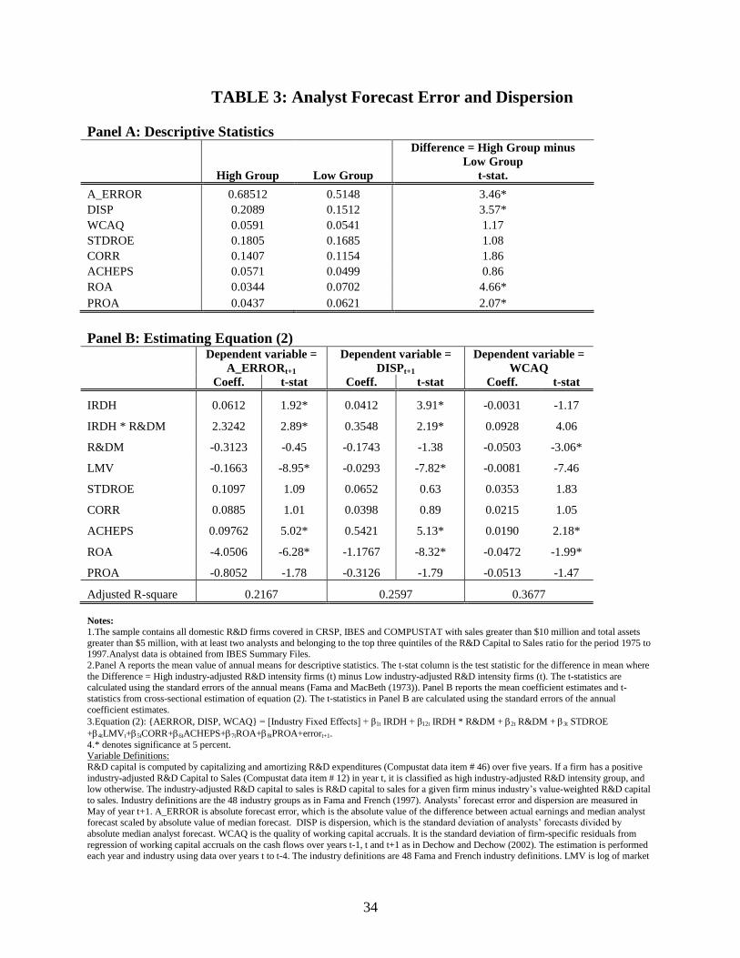
TABLE 3: Analyst Forecast Error and Dispersion

Panel A: Descriptive Statistics



Low Group

t-stat.

A_ERROR 0.68512 0.5148 3.46*

DISP 0.2089 0.1512 3.57*

WCAQ 0.0591 0.0541 1.17

STDROE 0.1805 0.1685 1.08

CORR 0.1407 0.1154 1.86

ACHEPS 0.0571 0.0499 0.86

ROA 0.0344 0.0702 4.66*

PROA 0.0437 0.0621 2.07*



A_ERRORt+1


DISPt+1


WCAQ

Coeff. t-stat Coeff. t-stat Coeff. t-stat

IRDH 0.0612 1.92* 0.0412 3.91* -0.0031 -1.17

IRDH * R&DM 2.3242 2.89* 0.3548 2.19* 0.0928 4.06

R&DM -0.3123 -0.45 -0.1743 -1.38 -0.0503 -3.06*

LMV -0.1663 -8.95* -0.0293 -7.82* -0.0081 -7.46

STDROE 0.1097 1.09 0.0652 0.63 0.0353 1.83

CORR 0.0885 1.01 0.0398 0.89 0.0215 1.05

ACHEPS 0.09762 5.02* 0.5421 5.13* 0.0190 2.18*

ROA -4.0506 -6.28* -1.1767 -8.32* -0.0472 -1.99*

PROA -0.8052 -1.78 -0.3126 -1.79 -0.0513 -1.47

Adjusted R-square 0.2167 0.2597 0.3677

Notes:


greater than $5 million, with at least two analysts and belonging to the top three quintiles of the R&D Capital to Sales ratio for the period 1975 to 1997.Analyst data is obtained from IBES Summary Files.

2. Panel A reports the mean value of annual means for descriptive statistics. The t-stat column is the test statistic for the difference in mean where

the Difference = High industry-adjusted R&D intensity firms (t) minus Low industry-adjusted R&D intensity firms (t). The t-statistics are calculated using the standard errors of the annual means (Fama and MacBeth (1973)). Panel B reports the mean coefficient estimates and t-

statistics from cross-sectional estimation of equation (2). The t-statistics in Panel B are calculated using the standard errors of the annual

coefficient estimates.

3. Equation (2): {AERROR, DISP, WCAQ} = [Industry Fixed Effects] + β1t IRDH + β12t IRDH * R&DM + 2t R&DM + 3t STDROE

+4tLMVt+5tCORR+6tACHEPS+7tROA+8tPROA+errort+1.

4. * denotes significance at 5 percent. Variable Definitions:



to sales. Industry definitions are the 48 industry groups as in Fama and French (1997). Analysts‘ forecast error and dispersion are measured in

May of year t+1. A_ERROR is absolute forecast error, which is the absolute value of the difference between actual earnings and median analyst forecast scaled by absolute value of median forecast. DISP is dispersion, which is the standard deviation of analysts‘ forecasts divided by

absolute median analyst forecast. WCAQ is the quality of working capital accruals. It is the standard deviation of firm-specific residuals from

regression of working capital accruals on the cash flows over years t-1, t and t+1 as in Dechow and Dechow (2002). The estimation is performed each year and industry using data over years t to t-4. The industry definitions are 48 Fama and French industry definitions. LMV is log of market

35

value of equity in April in billions. Market value of equity is share price at April multiplied by shares outstanding. STDROE is standard deviation

of return on equity (ROE) in preceding five-year period. Return on equity is earnings before extraordinary items (data18) divided by book value of equity (Compustat data item # 60). ACHEPS is absolute value of change in earnings per share (Compustat data item # 58) divided by share

price. CORR is the Pearson correlation between annual return and ROE in preceding five-year period. ROA is return on assets defined as

earnings before extraordinary items divided by total assets (Compustat data item # 6). PROA is the average of five years earnings divided by average of five year total assets. R&DM is R&D expenditure per share divided by share price.

36

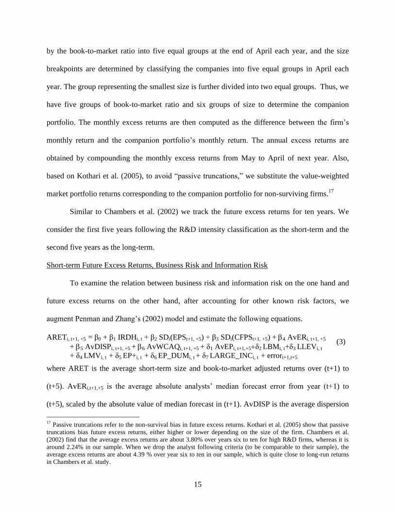
Table 4: Future Short-term Excess Returns



Difference = High minus Low

t-stat.

ARETt+1, +5) 0.0525 0.0249 2.21*

SD(EPSt+1, +5) 0.0319 0.0293 1.72

SD(CFPSt+1, +5) 0.0321 0.0345 -1.36

AvERi, t+1, +5 0.6532 0.5411 3.98*

AvDISPi, t+1, +5 0.1931 0.1536 3.95*

AvEPt+1, t+5 0.0513 0.0689 -1.90

AvWCAQt+1, t+5 0.0578 0.0551 0.86


Coeff t-stat. Coeff t-stat.

Intercept -0.0201 -2.58* -0.01209 -3.97*

IRDHt 0.0234 4.69* 0.0318 5.35*

STD(EPSt+1, t+5) 1.0241 5.21*

STD(CFPSt+1, t+5) -0.1061 -1.19

AvERi, t+1, +5 0.0279 1.39

AvDISPi, t+1, +5 0.1761 4.11*

AvWCAQt+1, t+5 -0.4012 -1.89

AvEPt+1, t+5 0.8761 12.42* 0.7324 8.21*

LBMt -0.0131 -2.11* -0.0042 -0.81

LLEVt 0.0002 0.23 0.0012 0.83

LMVt -0.0015 -0.81 -0.0083 -4.53*

EP(+)t -0.1621 -1.81 -0.1942 -1.89

EP_DUMt -0.0060 -0.52 0.0160 1.76

LARGE_INCt 0.0178 1.97* 0.0183 2.05*

Mean Adjusted R-square 0.2671 0.1708

Notes:

1. The sample contains all domestic R&D firms covered in CRSP, IBES and COMPUSTAT with sales greater than $10 million and total assets greater than $5 million, with at least two analysts and belonging to the top three quintiles of the R&D Capital to Sales ratio for the period 1975 to

1997.

2. Equation (5): ARETi, t+1, +5 = β0 + β1 IRDHi, t + β2 SDi(EPSt+1, +5) + β3 SDi(CFPSt+1, +5) + 4 AvFERi, t+1, +5 + 5 AvDISPi, t+1, +5 + 6 AvWCAQi, t+1, +5 + δ1 AvEPi, t+1, +5 + δ2 LBMi, t + δ3 LLEVi, t + δ4 LMVi, t + δ5 EP+i, t + δ6 EP_DUMi, t + δ7 LARGE_INCi, t + errort+1,t+5

3. The t-statistics are calculated using the standard errors of the annual coefficient estimates based on Fama and MacBeth (1973) procedure.

4. All variables except the dependant variable are winsorized at 1% and 99% of the annual distributions. 5. * denotes significance at 5 percent level.


R&D capital is computed by capitalizing and amortizing R&D expenditures (Compustat data item # 46) over five years. If a firm has a positive industry-adjusted R&D Capital to Sales (Compustat data item # 12) in year t, it is classified as high industry-adjusted R&D intensity group, and

37

low otherwise. The industry-adjusted R&D capital to sales is R&D capital to sales for a given firm minus industry‘s value-weighted R&D capital

to sales. Industry definitions are the 48 industry groups as in Fama and French (1997). IRDH is one if a firm is classified in the high group. ARETt+1, +5 is the average of the excess returns over short horizon (i.e. from (t+1) to (t+5)). The excess returns are size and book-to-market

adjusted returns. The excess returns are computed using the companion portfolio approach. Each firm in the sample is assigned to a companion

portfolio based on its ranking by size and book-to-market. For the companion portfolio the book-to-market ratios are classified into five equal groups at the end of April each year; the size breakpoints are determined by classifying the NYSE companies into five equal groups in April each

year. The group representing the smallest size is further divided into two equal groups. The monthly excess returns are then computed as the

difference the firm‘s monthly return minus the companion portfolio‘s monthly return. The annual excess returns are obtained by compounding the monthly excess returns from May to April of next year. SD(EPS) is the standard deviation of earnings per share (as defined in Table 2) over the

short- and long-terms scaled by stock price. SD(CFPS) is the standard deviation of cash flow from operations (as defined in Table 2) over the

short- and long-terms scaled by stock price. AvEP is the average earnings over the short- and long-terms scaled by share price. Analyst forecast error and dispersion AvER is the average absolute analysts‘ forecast error over the short- and long-terms scaled by absolute median analyst

forecast. Analysts‘ forecast error is the median analyst forecast minus actual earnings. AvDISP is the average dispersion in analyst forecasts over

the short- and long-terms scaled by absolute median analyst forecast in year t+1. All analyst forecast variables are measured in May from IBES Summary Files. AvWCAQ is the mean of WCAQ from t+1 to t+5. WCAQ is the quality of working capital accruals. It is the standard deviation

of firm-specific residuals from regression of working capital accruals on the cash flows over years t-1, t and t+1 as in Dechow and Dechow

(2002). The estimation is performed each year and industry using data over years t to t-4. The industry definitions are 48 Fama and French industry definitions. EP(+) is the earnings-to-price ratio if EP is positive and zero otherwise. Earning-to-price ratio is earnings before

extraordinary items (Compustat data item # 18) divided by market value of equity. AvEP is the mean of earnings-to-price ratio over the period

specified in the subscript. EP_DUM is one if the current earnings to price ratio is negative. LBM is the log of book-to-market ratio. Book-to-

market ratio is book value of equity (Compustat data item # 60) divided by market value of equity. LMV is the natural logarithm of the market

value of equity in April. LLEV is natural logarithm of the ratio of book value of debt (Compustat data item # 9 plus Compustat data item # 34) to

the market value of equity plus debt. LARGE_INC is an indicator variable which equals one if the firm has R&D intensity (R&D to asset and R&D to sales ratios) of at least 5%, the change in R&D to asset ratio and dollar value of R&D is at least 5% (i.e. increasing R&D to asset ratio

from 5% to at least 5.25%).

38

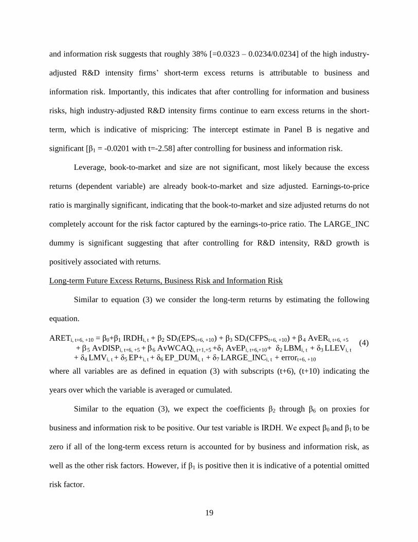
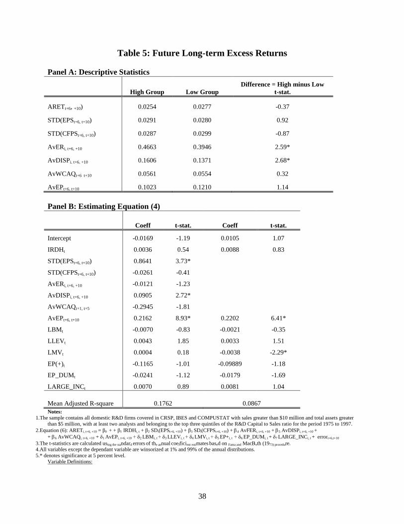
Table 5: Future Long-term Excess Returns



Difference = High minus Low

t-stat.

ARETt+6, +10) 0.0254 0.0277 -0.37

STD(EPSt+6, t+10) 0.0291 0.0280 0.92

STD(CFPSt+6, t+10) 0.0287 0.0299 -0.87

AvERi, t+6, +10 0.4663 0.3946 2.59*

AvDISPi, t+6, +10 0.1606 0.1371 2.68*

AvWCAQt+6 t+10 0.0561 0.0554 0.32

AvEPt+6, t+10 0.1023 0.1210 1.14


Coeff t-stat. Coeff t-stat.

Intercept -0.0169 -1.19 0.0105 1.07

IRDHt 0.0036 0.54 0.0088 0.83

STD(EPSt+6, t+10) 0.8641 3.73*

STD(CFPSt+6, t+10) -0.0261 -0.41

AvERi, t+6, +10 -0.0121 -1.23

AvDISPi, t+6, +10 0.0905 2.72*

AvWCAQt+1, t+5 -0.2945 -1.81

AvEPt+6, t+10 0.2162 8.93* 0.2202 6.41*

LBMt -0.0070 -0.83 -0.0021 -0.35

LLEVt 0.0043 1.85 0.0033 1.51

LMVt 0.0004 0.18 -0.0038 -2.29*

EP(+)t -0.1165 -1.01 -0.09889 -1.18

EP_DUMt -0.0241 -1.12 -0.0179 -1.69

LARGE_INCt 0.0070 0.89 0.0081 1.04

Mean Adjusted R-square 0.1762 0.0867

Notes:

1. The sample contains all domestic R&D firms covered in CRSP, IBES and COMPUSTAT with sales greater than $10 million and total assets greater

than $5 million, with at least two analysts and belonging to the top three quintiles of the R&D Capital to Sales ratio for the period 1975 to 1997. 2. Equation (6): ARETi, t+6, +10 = β0 + + β1 IRDHi, t + β2 SDi(EPSt+6, +10) + β3 SDi(CFPSt+6, +10) + 4 AvFERi, t+6, +10 + 5 AvDISPi, t+6, +10 +

+ 6 AvWCAQi, t+6, +10 + δ1 AvEPi, t+6, +10 + δ2 LBMi, t + δ3 LLEVi, t + δ4 LMVi, t + δ5 EP+i, t + δ6 EP_DUMi, t + δ7 LARGE_INCi, t + errort+6,t+10

3. The t-statistics are calculated using the standard errors of the annual coefficient estimates based on Fama and Maceth (1973) procedure. 4. All variables except the dependant variable are winsorized at 1% and 99% of the annual distributions.



39



to sales. Industry definitions are the 48 industry groups as in Fama and French (1997). IRDH is one if a firm is classified in the high group.

ARETt+6, +10 is the average of the excess returns over long horizon (i.e. from (t+6) to (t+10)). The excess returns are size and book-to-market adjusted returns. The excess returns are computed using the companion portfolio approach. Each firm in the sample is assigned to a companion

portfolio based on its ranking by size and book-to-market. For the companion portfolio the book-to-market ratios are classified into five equal

groups at the end of April each year; the size breakpoints are determined by classifying the NYSE companies into five equal groups in April each year. The group representing the smallest size is further divided into two equal groups. The monthly excess returns are then computed as the

difference the firm‘s monthly return minus the companion portfolio‘s monthly return. The annual excess returns are obtained by compounding the

monthly excess returns from May to April of next year. SD(EPS) is the standard deviation of earnings per share (as defined in Table 2) over the short- and long-terms scaled by stock price. SD(CFPS) is the standard deviation of cash flow from operations (as defined in Table 2) over the

short- and long-terms scaled by stock price. AvEP is the average earnings over the short- and long-terms scaled by share price. Analyst forecast

error and dispersion AvER is the average absolute analysts‘ forecast error over the short- and long-terms scaled by absolute median analyst forecast. Analysts‘ forecast error is the median analyst forecast minus actual earnings. AvDISP is the average dispersion in analyst forecasts over

the short- and long-terms scaled by absolute median analyst forecast in year t+1. All analyst forecast variables are measured in May from IBES

Summary Files. AvWCAQ is the mean of WCAQ from t+6 to t+10. WCAQ is the quality of working capital accruals. It is the standard deviation of firm-specific residuals from regression of working capital accruals on the cash flows over years t-1, t and t+1 as in Dechow and Dechow

(2002). The estimation is performed each year and industry using data over years t to t-4. The industry definitions are 48 Fama and French

industry definitions. EP(+) is the earnings-to-price ratio if EP is positive and zero otherwise. Earning-to-price ratio is earnings before

extraordinary items (Compustat data item # 18) divided by market value of equity. AvEP is the mean of earnings-to-price ratio over the period

specified in the subscript. EP_DUM is one if the current earnings to price ratio is negative. LBM is the log of book-to-market ratio. Book-to-

market ratio is book value of equity (Compustat data item # 60) divided by market value of equity. LMV is the natural logarithm of the market value of equity in April. LLEV is natural logarithm of the ratio of book value of debt (Compustat data item # 9 plus Compustat data item # 34) to

the market value of equity plus debt. LARGE_INC is an indicator variable which equals one if the firm has R&D intensity (R&D to asset and

R&D to sales ratios) of at leat 5%, the change in R&D to asset ratio and dollar value of R&D is at least 5% (i.e. increasing R&D to asset ratio from 5% to at least 5.25%).

40

TABLE 6: Management Forecasts and Future Excess Returns

Equation (5)

Equation (5) without

Business and

Information Risk

Equation (5)

without Guidance,

Leader Interaction

and Business and

Information Risk

Variable Coeff. t-stat Coeff. t-stat Coeff. t-stat

IRDHt 0.0432 3.71* 0.0451 3.78* 0.0417 3.57*

LN_FORCSTt 0.0023 0.15 0.0021 0.10 -0.0162 -1.82

LN_FORCSTt * IRDHt -0.0242 -1.66 -0.0293 -1.91*

STDi(EPSt+1, t+3) 0.9769 4.98*

STDi(CFPSt+1, t+3) 0.0569 0.51

AvERi, (t+1, +3) 0.0318 2.04*

AvDISPi, t+1, +3 0.1171 1.99*

AvWCAQt+1, t+3 -0.2655 -1.75

AvEPt+1, t+3 0.4879 8.05* 0.2845 5.96* 0.2745 5.71*

LBMt -0.0321 -2.98* -0.0274 -2.81* -0.0289 -2.93*

LLEVt 0.0038 0.79 0.0030 0.60 0.0037 0.75

LMVt -0.0209 -4.31* -0.0275 -7.18* -0.0269 -6.08*

EP(+)t -0.3962 -1.79 -0.3574 -1.87 -0.3765 -1.89

EP_DUMt -0.0192 -1.03 -0.0185 -0.62 -0.0178 -0.69

LARGE_INCt 0.0191 2.02* 0.0209 2.18* 0.0211 2.17*

Adjusted R-square 0.2045 0.1441 0.1432

Notes:


greater than $5 million, with at least two analysts and belonging to the top three quintiles of the R&D Capital to Sales ratio for the period 1994

to 2001. 2. Equation (5): ARETi, t+1,t+3 = [Year Dummies] + β1IRDHi, t + β2LN_FORCSTi, t + β2D LN_FORCSTi, t IRDH i, t + β3 STD(EPS t+1, t+3)

+ β4 STD(CFPS t+1, t+3) + β5 AvERi, t+1, t+3 + β6 AvDISPi, t+1, t+3 + β7 AvEPi, t+1, t+3 +8 AvWCAQi, t+1, t+3

+ β9 LBMi, t + β10 LLEVi, t + β11 LMVi, t + β12 EP+i, t + β13 EP_DUMi, t + β14LARGE_INCi, t + errort+1,t+3. 3. The t-statistics are calculated using the standard errors obtained from the Huber-White procedure (Petersen (2005)).

4. All variables except the dependant variable are winsorized at 1% and 99% of the annual distributions.




industry-adjusted R&D Capital to Sales (Compustat data item # 12) in year t, it is classified as high industry-adjusted R&D intensity group, and

low otherwise. The industry-adjusted R&D capital to sales is R&D capital to sales for a given firm minus industry‘s value-weighted R&D capital

to sales. Industry definitions are the 48 industry groups as in Fama and French (1997). ARETi,t+1,t+3 is the average size and book-to-market adjusted returns over three year period after portfolio formation (from t+1 to t+3). The calculation of excess returns is described in Table 4. IRDH

is an indicator variable which equals one if a firm is classified in the high group in year t. LN_FORCST is log of the number of management

forecasts in a year t from FIRSTCALL. SD(EPS) is the standard deviation of earnings per share (as defined in Table 2) over years t+1 to t+3 scaled by stock price. SD(CFPS) is the standard deviation of cash flow from operations (as defined in Table 2) over years t+1 to t+3 scaled by

stock price. AvEP is the average earnings over years t+1 to t+3 scaled by share price. Analyst forecast error and dispersion AvER is the average

absolute analysts‘ forecast error over years t+1 to t+3 scaled by absolute median analyst forecast. Analysts‘ forecast error is the median analyst forecast minus actual earnings. AvDISP is the average dispersion in analyst forecasts over years t+1 to t+3 scaled by absolute median analyst

forecast in year t+1. All analyst forecast variables are measured in May from IBES Summary Files. EP(+) is the earnings-to-price ratio if EP is

positive and zero otherwise. Earning-to-price ratio is earnings before extraordinary items (Compustat data item #18) divided by market value of

41

equity. AvEP is the mean of earnings-to-price ratio over the period specified in the subscript. AvWCAQ is the mean of WCAQ from t+1 to t+3.

WCAQ is the quality of working capital accruals. It is the standard deviation of firm-specific residuals from regression of working capital accruals on the cash flows over years t-1, t and t+1 as in Dechow and Dechow (2002). The estimation is performed each year and industry using

data over years t to t-4. The industry definitions are 48 Fama and French industry definitions. EP_DUM is one if the current earnings to price

ratio is negative. LBM is the log of book-to-market ratio. Book-to-market ratio is book value of equity (Compustat data item # 60) divided by market value of equity. LMV is the natural logarithm of the market value of equity in April. LLEV is natural logarithm of the ratio of book value

of debt (Compustat data item # 9 plus Compustat data item # 34) to the market value of equity plus debt, both at the end of year t. LARGE_INC

is an indicator variable which equals one if the firm has R&D intensity (R&D to asset and R&D to sales ratios) of at least 5%, the change in R&D to asset ratio and dollar value of R&D is at least 5% (i.e. increasing R&D to asset ratio from 5% to at least 5.25%).

Date post:	27-May-2018
Category:	Documents
Upload:	lamquynh
View:	215 times
Download:	0 times

Is R&D Mispriced or Properly Risk-Adjusted?raw.rutgers.edu/docs/intangibles/Papers/Is...

Documents