Is the cosmological coincidence a problem? Navin Sivanandam * African Institute for Mathematical Sciences, Muizenberg, 7945 Cape Town, South Africa (Received 14 September 2012; published 11 April 2013) The matching of our epoch of existence with the approximate equality of the dark energy and dark matter densities is an apparent further fine-tuning, beyond the already troubling 120 orders of magnitude that separate dark energy from the Planck scale. In this paper I will argue that this coincidence is not a fine-tuning problem, but instead an artifact of anthropic selection. Rather than assuming observations are equally likely in all epochs, one should insist that measurements of a quantity be typical amongst all such measurements. As a consequence, particular observations will reflect the epoch in which they are most easily made. In the specific case of cosmology, most measurements of dark energy and dark matter will be done during an epoch when large numbers of linear modes are available to observers, so we should not be surprised to be living at such a time. This idea is made precise in a particular model for the probability distribution for r min ð m ; m Þ, where it is shown that if pðrÞ½NðrÞ b [where NðrÞ is the number of linear modes, and b is some arbitrary positive power], the probability that r is greater than its observed value of 0.4 is close to 1. Thus the cosmological coincidence is no longer problematic. DOI: 10.1103/PhysRevD.87.083514 PACS numbers: 98.80.k, 95.36.+x I. INTRODUCTION A. The coincidence problem We live during a particularly interesting cosmological epoch; not only are our skies filled with the riches of the early universe, we are also fortunate enough to be living just as the era of matter gives way to that of dark energy. Somewhat more prosaically, we observe that the fractional densities of matter and dark energy are about the same: m (the i are defined as i ¼ & i =& crit , where i denotes the particular component of the universe and & crit is the time-dependent critical density). This ‘‘coincidence problem’’ is often viewed as a challenge for models of dark energy, and even if not quite as troubling as the problem of the magnitude of dark energy, explaining the coincidence in question is far from straightforward [1–3]. The apparent problem is starkly evident in Fig. 1, which shows the evolutions of the fractional densities of the various components of the cosmological fluid as functions of the logarithm of the scale factor a. Notice that only in an uncomfortably narrow band of log a are m and comparable. To make this discomfiture more precise I am going to follow Lineweaver and Egan in Ref. [4] and define the useful parameter, r, r ¼ min m ; m : (1) The current value of r is around 0.4, and the coincidence problem can be rephrased as a question about the proba- bility of finding r * 0:4. As Lineweaver and Egan point out, the expected value of r depends on one’s prior for pðaÞ, the probability distribution for when one expects to live. Figure 2 (where I have replicated similar plots from Ref. [4]) provides a stark visual representation of this prior dependence. The miracle of ‘‘Why now?’’ is rather less dramatic if the prior probability of our existence is flat in linear rather than log time, although the problem is still significant if we speculate on why we are not living in the far future. Regardless of the choice of prior, an examination of the shape of the plots makes it clear that the coincidence problem results from the fact that r approaches zero at large and small a, and it is at one or both of these values that most of the probability lies, assuming that one takes a flat prior for the x-axis position at which we happen to live. If one assumes that pðln aÞ or pðaÞ is flat, the probability of measuring r 1 depends on time cutoffs (the details of these calculations can be found in Appendix A), today 10 0 10 20 Log a 0.2 0.4 0.6 0.8 1.0 FIG. 1. The evolution of the different components of the universe, as a function of log a. The dashed line denotes r , the dotted line m , and the solid line . The shaded grey region covers the short epoch (that we happen to live in) where and m are comparable in magnitude. * [email protected]PHYSICAL REVIEW D 87, 083514 (2013) 1550-7998= 2013=87(8)=083514(11) 083514-1 Ó 2013 American Physical Society
Transcript
Is the cosmological coincidence a problem?
Navin Sivanandam*
African Institute for Mathematical Sciences, Muizenberg, 7945 Cape Town, South Africa(Received 14 September 2012; published 11 April 2013)
The matching of our epoch of existence with the approximate equality of the dark energy and dark
matter densities is an apparent further fine-tuning, beyond the already troubling 120 orders of magnitude
that separate dark energy from the Planck scale. In this paper I will argue that this coincidence is not a
fine-tuning problem, but instead an artifact of anthropic selection. Rather than assuming observations are
equally likely in all epochs, one should insist that measurements of a quantity be typical amongst all such
measurements. As a consequence, particular observations will reflect the epoch in which they are most
easily made. In the specific case of cosmology, most measurements of dark energy and dark matter will be
done during an epoch when large numbers of linear modes are available to observers, so we should not be
surprised to be living at such a time. This idea is made precise in a particular model for the probability
distribution for r � min ð�m
��;��
�mÞ, where it is shown that if pðrÞ � ½NðrÞ�b [where NðrÞ is the number of
linear modes, and b is some arbitrary positive power], the probability that r is greater than its observed
value of 0.4 is close to 1. Thus the cosmological coincidence is no longer problematic.
We live during a particularly interesting cosmologicalepoch; not only are our skies filled with the riches of theearly universe, we are also fortunate enough to be livingjust as the era of matter gives way to that of dark energy.Somewhat more prosaically, we observe that the fractionaldensities of matter and dark energy are about the same:�m ��� (the �i are defined as �i ¼ �i=�crit, where idenotes the particular component of the universe and �crit
is the time-dependent critical density). This ‘‘coincidenceproblem’’ is often viewed as a challenge for models of darkenergy, and even if not quite as troubling as the problem ofthe magnitude of dark energy, explaining the coincidencein question is far from straightforward [1–3].
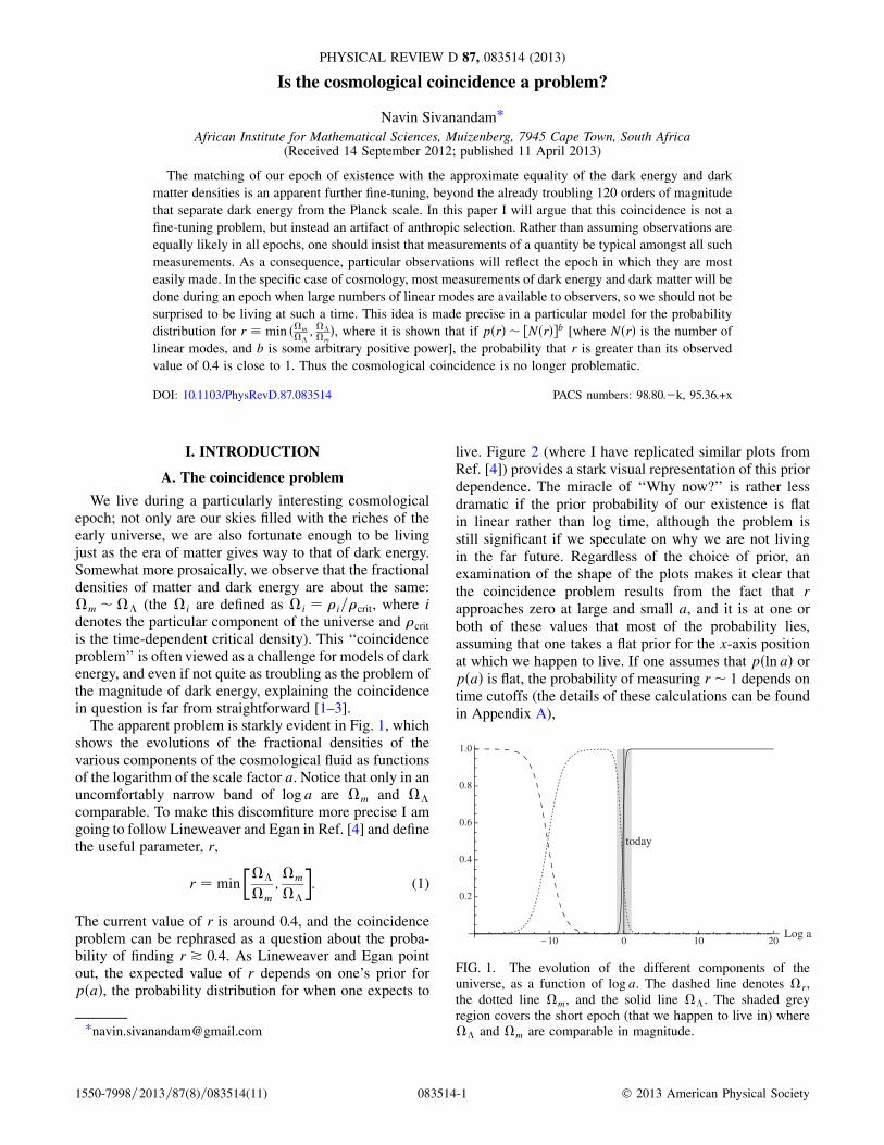
The apparent problem is starkly evident in Fig. 1, whichshows the evolutions of the fractional densities of thevarious components of the cosmological fluid as functionsof the logarithm of the scale factor a. Notice that only in anuncomfortably narrow band of log a are �m and ��
comparable. To make this discomfiture more precise I amgoing to follow Lineweaver and Egan in Ref. [4] and definethe useful parameter, r,
r ¼ min
���
�m
;�m
��
�: (1)
The current value of r is around 0.4, and the coincidenceproblem can be rephrased as a question about the proba-bility of finding r * 0:4. As Lineweaver and Egan pointout, the expected value of r depends on one’s prior forpðaÞ, the probability distribution for when one expects to
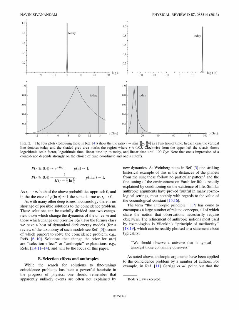
live. Figure 2 (where I have replicated similar plots fromRef. [4]) provides a stark visual representation of this priordependence. The miracle of ‘‘Why now?’’ is rather lessdramatic if the prior probability of our existence is flatin linear rather than log time, although the problem isstill significant if we speculate on why we are not livingin the far future. Regardless of the choice of prior, anexamination of the shape of the plots makes it clear thatthe coincidence problem results from the fact that rapproaches zero at large and small a, and it is at one orboth of these values that most of the probability lies,assuming that one takes a flat prior for the x-axis positionat which we happen to live. If one assumes that pðln aÞ orpðaÞ is flat, the probability of measuring r� 1 depends ontime cutoffs (the details of these calculations can be foundin Appendix A),
today
10 0 10 20Log a
0.2
0.4
0.6
0.8
1.0
FIG. 1. The evolution of the different components of theuniverse, as a function of log a. The dashed line denotes �r,the dotted line �m, and the solid line ��. The shaded greyregion covers the short epoch (that we happen to live in) where�� and �m are comparable in magnitude.*[email protected]
PHYSICAL REVIEW D 87, 083514 (2013)
1550-7998=2013=87(8)=083514(11) 083514-1 � 2013 American Physical Society
As tf ! 1 both of the above probabilities approach 0, and
in the the case of pðlnaÞ � 1 the same is true as ti ! 0.As with many other deep issues in cosmology there is no
shortage of possible solutions to the coincidence problem.These solutions can be usefully divided into two catego-ries: those which change the dynamics of the universe andthose which change our prior for pðaÞ. For the former classwe have a host of dynamical dark energy models (for areview of the taxonomy of such models see Ref. [5]), someof which purport to solve the coincidence problem, e.g.,Refs. [6–10]. Solutions that change the prior for pðaÞare ‘‘selection effect’’ or ‘‘anthropic’’ explanations, e.g.,Refs. [3,4,11–14], and will be the focus of this paper.
B. Selection effects and anthropics
While the search for solutions to fine-tuning/coincidence problems has been a powerful heuristic inthe progress of physics, one should remember thatapparently unlikely events are often not explained by
new dynamics. As Weinberg notes in Ref. [3] one strikinghistorical example of this is the distances of the planetsfrom the sun; these follow no particular pattern1 and thefine-tuning of the environment on Earth for life is readilyexplained by conditioning on the existence of life. Similaranthropic arguments have proved fruitful in many cosmo-logical settings, most notably with regards to the value ofthe cosmological constant [15,16].The term ‘‘the anthropic principle’’ [17] has come to
encompass a large number of related concepts, all of whichshare the notion that observations necessarily requireobservers. The refinement of anthropic notions most usedby cosmologists is Vilenkin’s ‘‘principle of mediocrity’’[18,19], which can be readily phrased as a statement abouttypicality:
‘‘We should observe a universe that is typical
amongst those containing observers.’’
As noted above, anthropic arguments have been appliedto the coincidence problem by a number of authors. Forexample, in Ref. [11] Garriga et al. point out that the
today
20 10 0 10 20 30log a
0.2
0.4
0.6
0.8
1.0r
today
30 20 10 0 10log t (s)
0.2
0.4
0.6
0.8
1.0
r
today
2 4 6 8 10 12 14t (Gyr)
0.2
0.4
0.6
0.8
1.0
r
today
20 40 60 80 100t (Gyr)
0.2
0.4
0.6
0.8
1.0
r
FIG. 2. The four plots (following those in Ref. [4]) show the the ratio r ¼ min ½��
�m;�m
��� as a function of time. In each case the vertical
line denotes today and the shaded grey area marks the region where r * 0:05. Clockwise from the upper left the x axis showslogarithmic scale factor, logarithmic time, linear time up to today, and linear time until 100 Gyr. Note that one’s impression of acoincidence depends strongly on the choice of time coordinate and one’s cutoffs.
1Bode’s Law excepted.
NAVIN SIVANANDAM PHYSICAL REVIEW D 87, 083514 (2013)
083514-2
coincidence between t0 (today) and t� (the time of darkenergy dominance) can be explained by assuming that thenumber of observers is proportional to the amount ofcarbon, so that most observations of the universe shouldtake place at the time of peak carbon production,t0 � tcarbon.
2 Noting that carbon peaks with star formation(tSFR � tcarbon), the authors find
t� � tG � tSFR � tcarbon � t0: (2)
tG is the time of galaxy formation, and the first twoapproximate equalities follow from anthropic (and other)details of structure formation. Thus the coincidencet� � t0 is explained.
A complementary analysis has been carried byLineweaver and Egan [4]. Here the authors consider theage distribution of terrestrial planets in the universe,imposing an additional offset (�tobs ¼ 4 Gyr) to accountfor the delay between forming a planet and life evolving.Within this framework they find that 68% of observersemerge earlier than us, while 32% emerge later. Thus weare typical amongst observers on terrestrial planets whotake around 4 billion years to evolve (the result is shown tobe robust for �tobs � 10 Gyr). The argument is extendedin Ref. [14] to apply to dynamical dark energy models,with similar conclusions.
Although the arguments above are perfectly satisfactoryanthropic explanations for the coincidence problem, theyare not without problems:
(a) Carbon bias. Carbon-based, planet-bound life maybe only a small (atypical) subset of potentialobservers.
(b) Sensitivity to late-time observers. If the typicaltimescale for intelligent life to form is much greaterthan that of carbon production or of terrestrial planetformation, then the above methods are both missingthe majority of observers.
(c) What about the multiverse? If we take the multiverseseriously, we should really be analyzing all parts ofit with a suitably small dark energy component, andnot fixing the detailed astrophysics.
One way to assuage these concerns is to be more generalin imposing selection effects. This can be done by focus-sing on the particular observation being made. To rephrasethe ‘‘principle of mediocrity’’:
‘‘A measurement of a quantity should be typical of
all possible measurements of that quantity.’’
To unpack that a little, consider the ratio r definedabove; when we ask that r not be finely tuned, we arereally asking that the value of r that we measure be typical
amongst all possible values that could be measured. Now,if the number of measurements is independent of time, weend up with the coincidence problem outlined above. If,however, measurements are easier in some epoch andharder in another and impossible in a third, we have totake that into account when asking what a typicalmeasurement of r is.Measuring r requires measuring both �m and ��, so
our distribution for typical values of r should account forhow easy it is to measure these quantities. As I shall arguebelow, this amounts to relating the prior distribution of r tothe ease of measuring the expansion of the universe.Essentially, in a universe with an accelerating componentand with a decoupling scale (below which matter no longerfollows the Hubble flow), there is a finite time when modesare available to do cosmology, and the number of modesavailable is peaked near the epoch of matter-� equality. Asa result the probability of �� ��m is close to 1.
C. The measure problem
I have so far left unmentioned the measure problem(see Ref. [20] for an up-to-date overview of measures).This oversight will be extended throughout most of thepaper, but it would be remiss of me not to spend a little timeon the issue.Themeasure problem arises in eternal inflation because of
the sensitivity of predictions to the choice of measure on thepopulated landscape of possible vacua. This sensitivity canhave profound consequences for one’s choice of prior forwhere and when observers should expect to find themselvesin the multiverse. Examples of measure-based solutions tothe coincidence problem can be found in Refs. [21,22].While in this paper I am focussing on an anthropic
approach, it is important to note that (as with all discus-sions of fine-tuning in cosmology) considerations of themeasure may also be relevant and could affect myconclusions. That said, a measure-blind approach to issuesof selection and fine-tuning in cosmology has not beenwithout its successes in the past [15], and the present workhopes to follow in those footsteps.
D. Organization
I shall provide the details of my argument that thenumber of linear modes provides a good proxy for pðrÞin Sec. II, following this with a derivation of the appro-priate probability distribution and a calculation ofPðr � 0:4Þ under various different assumptions. Afterthis, in Sec. III, I will discuss the conclusions one mightdraw from this sort of reasoning, along with a myriad ofcaveats and qualifications.
II. MEASURING r
To make the above discussion on measuring r moreprecise, let us begin by considering how a general observer
2This, of course, makes the reasonable assumption that oncosmological scales the timescale of intelligent life evolvingfrom the available carbon can be ignored.
IS THE COSMOLOGICAL COINCIDENCE A PROBLEM? PHYSICAL REVIEW D 87, 083514 (2013)
083514-3
may go about measuring �� and �m. Because matterclumps, its presence can be detected through the motionsof luminous test particles moving in the potential well of aparticular clump of matter. As such, sufficiently clevercosmologists armed with sufficiently advanced instru-ments and sufficiently generous funding grants can locateand ‘‘weigh’’ clumps of matter. Then, by adding the massesof these clumps together the aforementioned cosmologistscan make reasonable estimates of �m during almost allcosmological epochs (with the obvious caveat that thisargument requires luminous matter to roughly track darkmatter).
Measuring ��, however, is a different story. Assumingthere are no significant spatial variations in the dark energydensity,�� can only be detected through measurements ofthe Hubble expansion. This expansion is detected throughobservations of the redshifts and distances of ‘‘objects’’that are not gravitationally bound to the observer. Thegreater the number of such objects, the easier it is tomeasure the expansion. Although ‘‘number of objects’’ isinherently a notion that depends on the cosmological andastrophysical details of the particular universe we findourselves in, one has a reasonable proxy in the numberof linear modes in the observer’s Hubble radius that arelarger than the largest gravitationally bound structure.
There are several reasons why the use of N (the numberof linear modes) is a good proxy for the number of objects.Firstly, it bounds the maximum number of independent(in the sense of the motion with the Hubble flow) objects.As well as the number of modes, N also counts the numberof volumes within a Hubble radius that can contain a single(at most) maximally sized bound structure; thus N boundsthe maximum number of such independent objects. Ofcourse, a) ‘‘maximum’’ is not the same as ‘‘number of’’and b) each of these independent volumes may containmany objects (for example, type Ia supernovae) which canbe used to measure distance. That said, so long as theuniverse is isotropic it is reasonable to assume that thenumber of objects should scale as N.
In addition to the above line of reasoning, we should alsonote that N directly characterizes our ability to measurecosmological parameters when we use the linear modesthemselves as probes, as with the cosmic microwave back-ground (and, in the future, with 21-cm observations).Although such measurements usually cannot constraindark energy by themselves (see Ref. [23] for an exampleof a cosmic microwave background-only constrainton dark energy), they are an important factor in ourability to accurately determine cosmological parameters,including r.
Finally, assuming an approximately scale-invariantspectrum (as one has in our Hubble volume and wouldhave in other Hubble volumes with an inflationary periodin their past) implies a correlation between the number oflinear modes and the number of objects. This follows since
with a scale-invariant spectrum the initial amount of powerat each scale is constant. Consequently, the number ofsmall objects useful for probing cosmology should scalewith N.There are, of course, many other factors that will affect
the ease of measuring r. However, on the grounds ofmaintaining generality, I am going to ignore most ofthem. One that might have a general applicability, though,is the ability to discriminate between different cosmolo-gies. In particular, the ability to tell an accelerating from anonaccelerating universe seems a prerequisite for measur-ing r, and this is not independent of the value of r. This willbe discussed in more detail below.In order to encompass a wider class of models than
simply vacuum energy, I shall present results for a cosmol-ogy consisting of matter with the equation of state p ¼ 0,and dark energy with the equation of state p ¼ w�, where�1 � w<�1=3. Then
H2 ¼ 1
3
��m0
�a0a
�3 þ ��0
�a0a
�3þ3w
�: (3)
Here, as below, the reduced Planck mass ð8�GÞ�1=2 hasbeen set equal to 1 and the subscript 0 denotes the timewhen the largest bound structure for a given observerenters the Hubble radius. I have also assumed that we arein a flat universe with �rad � 1.3
I should emphasize that while the rest of this section islittered with details of calculations, multiple plots, andseveral actual numbers, these are somewhat incidental tothe larger argument. The purpose of this paper is not toclaim that the probability of measuring r has some valuethat can be calculated given a suitably detailed model ofphysicists and their methods of observation. Rather, I wishto point out that the apparent fine-tuning of the coincidenceproblem is an artifact of an error in the typical choice ofprior for the epoch in which cosmological observers live.Once this error is corrected, by choosing an appropriateprior for the epoch of measurement, one finds that the fine-tuning has vanished. The particular analysis and numericalresults that follow should thus be considered as evidencefor this point of view, and a representative (rather thanfaithful) model of reality.
A. Number of measurements
The number of independent measurements that can bemade of the expansion of the universe depends on thenumber of modes within a Hubble radius that are notdecoupled from the Hubble flow. In a universe of matterand dark energy, modes enter the Hubble volume of anobserver during the epoch of matter domination and exitduring the epoch of dark energy domination. Thus there is
3It would take a particularly delicate fine-tuning to arrange aperiod of radiation domination close to the time of matter/darkenergy domination.
NAVIN SIVANANDAM PHYSICAL REVIEW D 87, 083514 (2013)
083514-4
only a finite period during which cosmological measure-ments can be made.
Because the definition of r varies with time it is useful towork with the quantities rm ¼ ��=�m and r� ¼ �m=��,
which are equal to r ¼ min ½��
�m;�m
��� when �� <�m and
�m <��, respectively. With these definitions, we have
H2 ¼ ��
3
�1
rmþ 1
�; �� ¼ ��0
�a0a
�3þ3w
;
rm ¼ r0
�a0a
�3w:
(4)
Let k� be the comoving wavenumber corresponding to thelargest bound structure seen by a given observer, andconsider the quantity k�=aH,
k�aH
¼ k�a0H0
0@1þ r0
r� 1
3w
0
1A1
2� r� 1
3wm
1þ rm
�12: (5)
If we set subscript-0 quantities to be at the initial timewhenthe mode corresponding to the largest bound structure isequal in size to the Hubble radius, then we have
k�aH
¼0@1þ r0
r� 1
3w
0
1A1
2� r� 1
3wm
1þ rm
�12: (6)
Cosmology is possible when the above quantity is largerthan 1. This is true, in the case of w ¼ �1, when
This range is somewhat larger for larger values ofw, as canbe seen in Fig. 3. The number of modes available forcosmology scales like the cube of Eq. (6),
Nm �0@1þ r0
r� 1
3w
0
1A3
2� r� 1
3wm
1þ rm
�32: (8)
Figure 3 shows the number of modes available to anobserver as a function of rm and of a. Note that whilechanging w affects the length of the period during whichcosmology can be done, the shape of the distribution ofmodes as a function of r or a is always strongly peaked andbroadly unchanged for different values of w.In order to calculate the probability Pðr � 0:4Þ, we will
also need the number of modes in terms of r� when�� >�m. This is given by
N� �0@1þ r0
r� 1
3w
0
1A3
2� r1þ 1
3w
�
1þ r�
�32: (9)
B. Probability distribution for r
To calculate the probability distribution function pðrÞ,we begin by constructing pðrjr � rmÞ and pðrjr � r�Þ.The probabilities should be proportional to a function ofthe number modes available,
There are several reasonable choices for the form of thefunction fi, depending on one’s model of measurement. Ongeneral grounds, one should expect the fi to be monotonic(measurement is clearly easier when more modes areavailable), but beyond that it is hard to justify a particularchoice of fi.Since the number of modes is maximized when r ¼ 1
(i.e., at the time of maximum coincidence), any pðrÞ
10 12 10 7 0.01 1000 108 1013rm
10
1000
105
107
109
N(rm)
1 1000 106 109 1012 1015a
10
1000
105
107
109
N(a)
FIG. 3. These two plots illustrate how the number of modes available to an observer changes as a function of rm and of a. In eachcase r0 ¼ 10�12 (which is approximately the value for our universe, if we assume dark energy is a pure cosmological constant).w ¼ �1 for the most finely dashed line and then�0:9,�0:8,�0:7, and�0:6 as the dashing increases in width. Note the increasing wincreases the amount of time available for cosmology but has little effect on the shape (and importantly the peakedness) of NðrmÞ.In each case the vertical line indicates the value of rm or a for current observers in our universe.
IS THE COSMOLOGICAL COINCIDENCE A PROBLEM? PHYSICAL REVIEW D 87, 083514 (2013)
083514-5
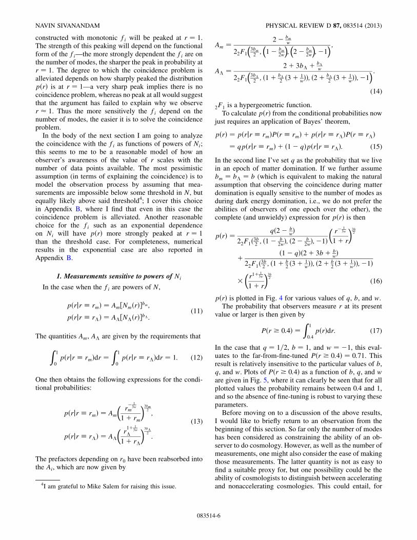
constructed with monotonic fi will be peaked at r ¼ 1.The strength of this peaking will depend on the functionalform of the fi—the more strongly dependent the fi are onthe number of modes, the sharper the peak in probability atr ¼ 1. The degree to which the coincidence problem isalleviated depends on how sharply peaked the distributionpðrÞ is at r ¼ 1—a very sharp peak implies there is nocoincidence problem, whereas no peak at all would suggestthat the argument has failed to explain why we observer 1. Thus the more sensitively the fi depend on thenumber of modes, the easier it is to solve the coincidenceproblem.
In the body of the next section I am going to analyzethe coincidence with the fi as functions of powers of Ni;this seems to me to be a reasonable model of how anobserver’s awareness of the value of r scales with thenumber of data points available. The most pessimisticassumption (in terms of explaining the coincidence) is tomodel the observation process by assuming that mea-surements are impossible below some threshold in N, butequally likely above said threshold4; I cover this choicein Appendix B, where I find that even in this case thecoincidence problem is alleviated. Another reasonablechoice for the fi such as an exponential dependenceon Ni will have pðrÞ more strongly peaked at r ¼ 1than the threshold case. For completeness, numericalresults in the exponential case are also reported inAppendix B.
In the second line I’ve set q as the probability that we livein an epoch of matter domination. If we further assumebm ¼ b� ¼ b (which is equivalent to making the naturalassumption that observing the coincidence during matterdomination is equally sensitive to the number of modes asduring dark energy domination, i.e., we do not prefer theabilities of observers of one epoch over the other), thecomplete (and unwieldy) expression for pðrÞ is then
pðrÞ ¼ qð2� bwÞ
22F1ð3b2 ; ð1� b2wÞ; ð2� b
2wÞ;�1Þ�r� 1
3w
1þ r
�3b2
þ ð1� qÞð2þ 3bþ bwÞ
22F1ð3b2 ; ð1þ b2 ð3þ 1
wÞÞ; ð2þ b2 ð3þ 1
wÞÞ;�1Þ
�r1þ 1
3w
1þ r
�3b2
(16)
pðrÞ is plotted in Fig. 4 for various values of q, b, and w.The probability that observers measure r at its present
value or larger is then given by
Pðr � 0:4Þ ¼Z 1
0:4pðrÞdr: (17)
In the case that q ¼ 1=2, b ¼ 1, and w ¼ �1, this eval-uates to the far-from-fine-tuned Pðr � 0:4Þ ¼ 0:71. Thisresult is relatively insensitive to the particular values of b,q, and w. Plots of Pðr � 0:4Þ as a function of b, q, and ware given in Fig. 5, where it can clearly be seen that for allplotted values the probability remains between 0.4 and 1,and so the absence of fine-tuning is robust to varying theseparameters.Before moving on to a discussion of the above results,
I would like to briefly return to an observation from thebeginning of this section. So far only the number of modeshas been considered as constraining the ability of an ob-server to do cosmology. However, as well as the number ofmeasurements, one might also consider the ease of makingthose measurements. The latter quantity is not as easy tofind a suitable proxy for, but one possibility could be theability of cosmologists to distinguish between acceleratingand nonaccelerating cosmologies. This could entail, for4I am grateful to Mike Salem for raising this issue.
NAVIN SIVANANDAM PHYSICAL REVIEW D 87, 083514 (2013)
083514-6
example, finding an expression for how the difference inthe luminosity-redshift relation between an acceleratingand decelerating cosmology varies as a function of r. Ifone did this, one would find a slightly greater pressuretowards large r when�m >�� and towards small r when�m <��. However, numerical investigations suggest thatthe probabilities are altered by around 10%, which wouldhave no effect on the above conclusions. Moreover, in theabsence of a compelling reason to do so, it is better tomodel selection effects with as little sensitivity to detailedphysics as possible.
III. CAVEATS AND CONCLUSIONS
The strengths and weaknesses of the above argument arereviewed below, but before we get to those, there are acouple of as yet undiscussed caveats that should be
mentioned. The first is that the reasoning used hereindoes not apply to dynamical dark energy models, where
the period of acceleration is temporary. Of course, this
simply means that the ‘‘Why now?’’ problem must be
added to the list of challenges such models face
(see Refs. [6–10] for examples of dynamical dark energy
models that attempt to explain the coincidence dynami-
cally). In addition, by not including�r in mymodel, I have
implicitly ignored the (possible) coincidence of our epoch
of existence and that of matter-radiation equality. Such a
coincidence is considerably milder in magnitude than that
of the dark energy and matter coincidence, with�r=�m �10�4. However, the naive expectation should be that this
ratio is close to its lowest possible value. There may well
be an anthropic explanation for this fine(ish)-tuning, but in
this paper it remains a mystery.
0.2 0.4 0.6 0.8 1.0r
0.2
0.4
0.6
0.8
1.0
1.2
1.4
0.2 0.4 0.6 0.8 1.0r
0.5
1.0
1.5
0.2 0.4 0.6 0.8 1.0r
0.2
0.4
0.6
0.8
1.0
1.2
p(r) p(r)p(r)
FIG. 4. The left-hand plot shows pðrÞ for various values of q (b ¼ 1, w ¼ �1): in order of increasing dash width, q ¼ 0, 1=4, 1=2,3=4, 1. In the middle the curves are for different values of b (q ¼ 1=2, w ¼ �1): in order of dash width, b ¼ 1=3, 2=3, 1, 2, 3. And onthe right we have varying w: in order of dash width we have w ¼ �1, �0:75, �0:5, �0:4, �0:35.
0.2 0.4 0.6 0.8 1.0q
0.65
0.70
0.75
0.80
0.85
0.90
0.5 1.0 1.5 2.0 2.5 3.0b
0.65
0.70
0.75
0.80
0.85
0.90
0.9 0.8 0.7 0.6 0.5 0.4w
0.65
0.70
0.75
0.80
P(r 0.4)
0.2 0.4 0.6 0.8 1.0q
0.5
0.6
0.7
0.8
0.5 1.0 1.5 2.0 2.5 3.0b
0.60
0.65
0.70
0.75
0.80
0.9 0.8 0.7 0.6 0.5 0.4w
0.60
0.65
0.70
0.75
0.80
P(r 0.4) P(r 0.4)
P(r 0.4) P(r 0.4) P(r 0.4)
FIG. 5. Plots of Pðr � 0:4Þ as functions (from left to right) of q, b, and w. The top left plot has b ¼ 1=3, 2=3, 1, 2, 3 in order ofincreasing dash width (w ¼ �1), while the bottom plot has w ¼ �1, �0:75, �0:5, �0:4, �0:35 (b ¼ 1) in order of increasing dashwidth. In the middle column, the top plot has q ¼ 0, 0.25, 0.5, 0.75, 1 as the dash width increases (w ¼ �1), and w varies as its left-hand neighbor in the bottom plot (q ¼ 0:5). Finally, in order of increasing dash width, the top right plot has b ¼ 1=3, 2=3, 1, 2, 3(q ¼ 0:5) and the bottom right plot has q ¼ 0, 0.25, 0.5, 0.75, 1 (b ¼ 1).
IS THE COSMOLOGICAL COINCIDENCE A PROBLEM? PHYSICAL REVIEW D 87, 083514 (2013)
083514-7
The calculations in the previous section demonstrate thatthe coincidence problem is an artifact of selection bias.This demonstration required the following assumptions:
(a) Selection effects are a sufficient explanation offine-tuning.
(b) An expectation that we are more likely to findourselves measuring r where most of the measure-ments of r are possible is a sensible selection effect.
(c) The frequency of measurements of r is correlatedwith the number of cosmological modes within asingle Hubble radius, NðrÞ.
(d) There are no other factors that have a significanteffect on the frequency of measurements of r.
With these assumptions the argument follows straight-forwardly: observers are more likely to measure r when itis easy to measure; r is easy to measure when there are lotsof modes available to the observer; there are lots of modesavailable to the observer when r is close to 1, Q.E.D. Ofcourse, there still remains the justification of the aboveassumptions. While the above points have been defended atthe relevant points in the body of the text, it is useful toreview the arguments before we finish.
Defenses of the anthropic principle are numerous, andthere is little I can offer that will persuade the unpersuadedreader. That said, I suppose it behoves one to try. Fine-tuning problems can, for the most part, be viewed as state-ments about selection effects, if not in real space then atleast in the space of possible worlds. This is especially truewith regards to the cosmological coincidence, where theproblem can be rephrased as, ‘‘If our epoch of existence isselected (log) uniformly in time, why are we so fortunate asto live in the epoch of matter and dark energy equality?’’All the principle of mediocrity states is that existence isnot selected from a uniform distribution and that we canmake reasonable deductions about what that distributionshould be.
Of course, making ‘‘reasonable’’ deductions is far from
straightforward. In this paper I have argued that cosmolo-
gists should expect to find themselves living in the epoch
when most cosmology can be done, and that furthermore,
this epoch is the one in which there are the greatest
number of visible modes. This argument for the correlation
between the number of modes and the number of measure-
ments contains an implicit assumption that there is bound
structure (which seems a reasonable requirement for
observers). I should also note that there are methods
(though somewhat constrained ones) to continue cosmol-
ogy after all else but the local structure has exited the
horizon; one such method is the measurement of cosmo-
logical parameters using hyper-velocity stars, discussed by
Loeb in Ref. [24]—in this paper I have ignored this pos-
sibility. With that said, precision cosmology will certainly
be harder in the future, even if it is not impossible.The use of only NðrÞ to construct pðrÞ can be defended
on several grounds. Firstly, incorporating an additional
dependence on the ease of discriminating between cos-mologies did not substantially change my conclusions.Secondly, the peakedness of NðrÞ suggests that it wouldtake a substantial anthropic counterweight to restore apressure to small values of r, and one has trouble conceiv-ing of what such an effect could be. Finally, the calculat-ion of NðrÞ requires little additional physics and ismostly insensitive to additional cosmological parameters(in particular, details of the spectrum, of structure forma-tion, of the physics of radiation, and so on); this suggeststhat marginalizing over additional parameters would noteffect the form of NðrÞ.The alert reader will have realized that I glossed over a
key point in my defense of the assumptions of this paper:why should cosmologists expect to live when cosmology iseasiest? Is not my whole argument trivial? Really all thathas been done is to show that we live in the era of engagingcosmology, without answering the question of why we livein interesting times.Well, in much the same way as students of climate
change were unlikely to be found before the climate startedchanging, so it is with cosmologists. In epochs wherecosmology is verging on the impossible, the questionsabout the apparent interestingness (or otherwise) of cos-mology are unlikely to be asked.We are fortunate enough to live in interesting times, but
if we did not, we would be blissfully unaware of that fact.
ACKNOWLEDGMENTS
I would like to thank Bruce Bassett, Rhiannon Gwyn,and Michael Salem for helpful discussions.
APPENDIX A: pðrÞ WITHOUTSELECTION EFFECTS
Let us begin by considering pðrÞ when pðaÞ � 1,
pðrÞ ¼ da
drpðaÞ � da
dr: (A1)
Noting that r� a3 when �m >�� and r� a�3 when�� >�m, this gives
pðrj�m >��Þ � r�2=3; pðrj�� >�mÞ � r�4=3:
(A2)
To calculate pðrÞ we also need Pð�m >��Þ andPð�� >�mÞ,
Pð�m >��Þ ¼Ra1aidaRaf
ai da¼ a1 � ai
af � ai� 0; (A3)
Pð�� >�mÞ ¼Rafa1 daRafai da
¼ af � a1af � ai
� 1: (A4)
NAVIN SIVANANDAM PHYSICAL REVIEW D 87, 083514 (2013)
083514-8
a1 is the value of a when r ¼ 1. The last approximateequality in each line corresponds to taking the limitai � a1 � af. Thus
Pðr � 0:4Þ ¼R10:4 r
�4=3drR1rfr�4=3dr
¼ 1:07
r�1=3f � 1
� a1af
� e�Htf :
(A5)
H is the asymptotic value of the Hubble constant for acosmological-constant-dominated universe, H2 ¼ �=3.A cutoff (rf, tf, af) is introduced in the normalization of
the probability to keep everything finite. As a result, onefinds that, because of the large future volume, the proba-bility of measuring r � 0:4 is exponentially small as afunction of the cutoff time.
Now let us consider pðrÞ when pðln aÞ � 1. With thedependence of r on a as before, this gives
pðrj�m >��Þ � r�1; pðrj�� >�mÞ � r�1: (A6)
Since pðaÞ � a�1, Pð�m >��Þ and Pð�� >�mÞ aregiven by
Pð�m >��Þ �ln a1
ai
lnafai
; Pð�� >�mÞ �ln
afa1
lnafai
:
Then for the probability that r � 0:4, one has
Pðr � 0:4Þ ¼ 1
lnafai
�Z 1
0:4r�1dr
� ln a1ai
� ln ri� ln
afa1
ln rf
!
� 1
lnafai
0@ ln a1
ai
�3 ln aia1
� lnafa1
�3 lnafa1
1A
� 1
lnafai
� 1
Htf � 23 ln
tit1
: (A7)
Once again the probability of measuring r�Oð1Þ isdetermined by the cutoffs. In this case both early- andlate-time cutoffs are important, though the sensitivity issomewhat less.
APPENDIX B: A DIFFERENT CHOICE FOR fi
1. Threshold
Instead of taking a power-law relationship between pðrÞand NðrÞ, one can take a threshold approach, where allmeasurements are considered equal when the number ofmodes available to the observer is greater than some mini-mum value.
To calculate the value of Pðr � 0:4Þ in such a model ofmeasurement requires more than just specifying a mini-mum number of modes; one also needs to define ‘‘equallylikely.’’ There are a number of different interpretations of
the assumption that measurements are equally probableafter the threshold number of modes has been exceeded.Three reasonable possibilities are pðrÞ ¼ const, pðaÞ ¼const, and pðln aÞ ¼ const. These will give different valuesof the amount (or otherwise) of fine-tuning inherent in ourmeasurements of r.Considering the w ¼ �1 case and setting the minimum
number of modes needed to observe r as n, one finds
The quantity r�1=20 is approximately equal to the maximum
number of modes that will ever be available to an observer,
so r1=20 n is the fraction of the maximal data available that is
needed to make an observation. In the first case above,Pðr � 0:4Þ is not finely tuned at all. In the second and thirdcases the tuning is worst if we assume n ¼ 1. For ouruniverse, where r0 � 10�12, this is a fine-tuning of�1=100 for pðaÞ ¼ const and �1=10 for pðlnaÞ ¼ const.
2. Exponential
pðrÞ can be readily constructed for an exponentialdependence of ease of measurement on the number oflinear modes, in the same fashion as for the power lawdiscussed in the main body of the paper. One obtains
pðrÞ ¼ Amq exp
�b
�r� 1
3w
1þ r
�32
�
þ A�ð1� qÞ exp�b
�r1þ 1
3w
1þ r
�32
�: (B2)
Am and A� are normalizations as before, chosen so thatR10 pðrjr � rmdrÞ ¼
R10 pðrjr � r�Þdr ¼ 1. b parame-
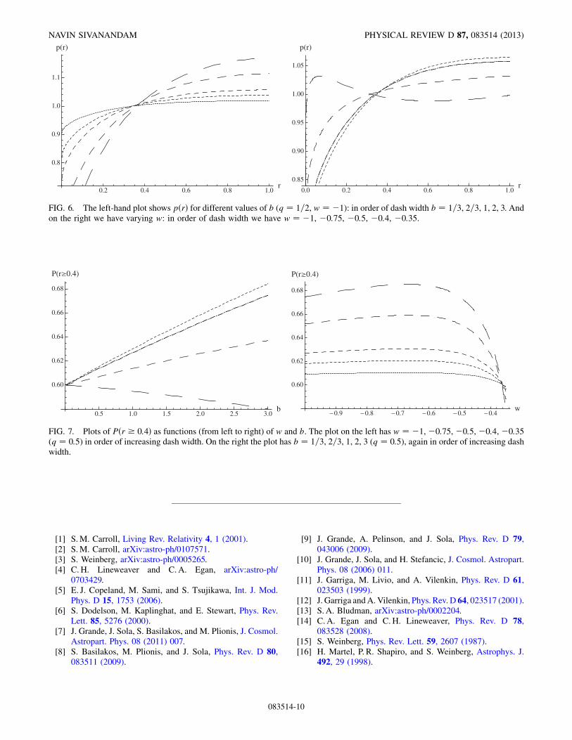
trizes that exponential—a larger b would imply observerswhose ability to measure expansion is more sensitive to thenumber of linear modes (as in the power-law case, I haveassumed that observers during matter and dark energydomination are similar in there ability to measureexpansion).Figure 6 contains plots of pðrÞ for various values of the
parameters. As with the power-law case much of theprobability lies close to r ¼ 1.Integrating the probability density from r ¼ 0:4 to r ¼ 1
will give Pðr � 0:4Þ, the probability that we live in auniverse at least as coincidental as ours. Figure 7 showsPðr � 0:4Þ for various parameter values. Note that for theparameters explored, Pðr � 0:4Þ is between around 0.5 and1, i.e., there is no coincidence problem.
IS THE COSMOLOGICAL COINCIDENCE A PROBLEM? PHYSICAL REVIEW D 87, 083514 (2013)
083514-9
[1] S.M. Carroll, Living Rev. Relativity 4, 1 (2001).[2] S.M. Carroll, arXiv:astro-ph/0107571.[3] S. Weinberg, arXiv:astro-ph/0005265.[4] C. H. Lineweaver and C.A. Egan, arXiv:astro-ph/
0703429.[5] E. J. Copeland, M. Sami, and S. Tsujikawa, Int. J. Mod.
Phys. D 15, 1753 (2006).[6] S. Dodelson, M. Kaplinghat, and E. Stewart, Phys. Rev.
Lett. 85, 5276 (2000).[7] J. Grande, J. Sola, S. Basilakos, and M. Plionis, J. Cosmol.
Astropart. Phys. 08 (2011) 007.[8] S. Basilakos, M. Plionis, and J. Sola, Phys. Rev. D 80,
083511 (2009).
[9] J. Grande, A. Pelinson, and J. Sola, Phys. Rev. D 79,043006 (2009).
[10] J. Grande, J. Sola, and H. Stefancic, J. Cosmol. Astropart.Phys. 08 (2006) 011.
[11] J. Garriga, M. Livio, and A. Vilenkin, Phys. Rev. D 61,023503 (1999).
[12] J. Garriga andA.Vilenkin, Phys. Rev. D 64, 023517 (2001).[13] S. A. Bludman, arXiv:astro-ph/0002204.[14] C. A. Egan and C.H. Lineweaver, Phys. Rev. D 78,
083528 (2008).[15] S. Weinberg, Phys. Rev. Lett. 59, 2607 (1987).[16] H. Martel, P. R. Shapiro, and S. Weinberg, Astrophys. J.
492, 29 (1998).
0.5 1.0 1.5 2.0 2.5 3.0b
0.60
0.62
0.64
0.66
0.68
P(r 0.4)
0.9 0.8 0.7 0.6 0.5 0.4w
0.60
0.62
0.64
0.66
0.68
P(r 0.4)
FIG. 7. Plots of Pðr � 0:4Þ as functions (from left to right) of w and b. The plot on the left has w ¼ �1, �0:75, �0:5,�0:4, �0:35(q ¼ 0:5) in order of increasing dash width. On the right the plot has b ¼ 1=3, 2=3, 1, 2, 3 (q ¼ 0:5), again in order of increasing dashwidth.
0.2 0.4 0.6 0.8 1.0r
0.8
0.9
1.0
1.1
p(r) p(r)
0.0 0.2 0.4 0.6 0.8 1.0r
0.85
0.90
0.95
1.00
1.05
FIG. 6. The left-hand plot shows pðrÞ for different values of b (q ¼ 1=2, w ¼ �1): in order of dash width b ¼ 1=3, 2=3, 1, 2, 3. Andon the right we have varying w: in order of dash width we have w ¼ �1, �0:75, �0:5, �0:4, �0:35.
NAVIN SIVANANDAM PHYSICAL REVIEW D 87, 083514 (2013)
[17] B. Carter, Gen. Relativ. Gravit. 43, 3225 (2011).[18] A. Vilenkin, Phys. Rev. Lett. 74, 846 (1995).[19] A. Vilenkin, arXiv:1108.4990.[20] B. Freivogel, Classical QuantumGravity 28, 204007 (2011).[21] R. Bousso, B. Freivogel, S. Leichenauer, and V.
Rosenhaus, Phys. Rev. D 84, 083517 (2011).
[22] R. Bousso, B. Freivogel, S. Leichenauer, and V.Rosenhaus, Phys. Rev. Lett. 106, 101301 (2011).
[23] B. D. Sherwin et al., Phys. Rev. Lett. 107, 021302(2011).
[24] A. Loeb, J. Cosmol. Astropart. Phys. 04 (2011)023.
IS THE COSMOLOGICAL COINCIDENCE A PROBLEM? PHYSICAL REVIEW D 87, 083514 (2013)