1 INTRODUCTIONIn 1958, economist A.W. Phillips discovered a strong negative correlation between the
money wage rate and the unemployment rate in the United Kingdom.1 Shortly after his find-ings were published, numerous studies confirmed that this relationship held in many devel-oped economies. For example, Samuelson and Solow (1960) demonstrated that the Phillips curve held in U.S. data, and they began to explore its policy implications.
The profession holds that the inverse relationship between unemployment and inflation implies a tradeoff between the two: low unemployment at the cost of higher inflation or low
A.W. Phillips’s discovery that inflation is negatively correlated with unemployment served as a heuristic model for conducting monetary policy; but the flattening of the Phillips curve post-1970 has divided debate on this empirical relation into two camps: “The Phillips curve is alive and well,” and “The Phillips curve is dead.” However, this dichotomy oversimplifies the issue. In this article, we apply spectral analysis to the U.S. inflation rate and unemployment rate to conduct a comprehensive analysis of the Phillips curve in the frequency domain. We find that in the very short run, there is no systemic relationship between inflation and unemployment; in the intermediate run, which includes the business cycle frequency, they are strongly negatively correlated; and in the very long run the Phillips curve is strongly positively sloped. Such an analysis of the frequency domain provides a natural demar-cation of frequency bands that allows us to recover the Phillips curve in the time domain by applying band-pass filters. Most importantly, we show how spectral analysis can be used to identify a “supply” (permanent) and a “demand” (nonpermanent) shock in the context of a vector autoregression and that demand shocks drive the Phillips curve. Finally, the phase spectral analysis also shows that despite the existence of the Phillips curve at the business cycle frequency under a demand shock, the mone-tary policy implications are not obvious, due to the unclear lead-lag relationship between inflation and unemployment. (JEL C100, E240, E310, E520, E580)
Federal Reserve Bank of St. Louis Review, Second Quarter 2020, 102(2), pp. 121-44. https://doi.org/10.20955/r.102.121-44
Brian Reinbold is a research associate and Yi Wen is an assistant vice president and economist at the Federal Reserve Bank of St. Louis.
122 Second Quarter 2020 Federal Reserve Bank of St. Louis REVIEW
inflation at the cost of higher unemployment. This tradeoff provides policymakers a menu of monetary policy prescriptions and also shows them how influencing nominal variables can affect the real economy. Monetary policy, for example, can adjust the money supply or nomi-nal interest rates to affect the price level and then through the Phillips curve affect employment. Because of the explanatory power of the Phillips curve, after its introduction, economists immediately incorporated it into structural models and this literature flourished and became an indispensable part of Keynesian economics.
However, the 1970s saw the Phillips curve breakdown, and the correlation in fact became positive. The U.S. experienced higher oil prices, and these adverse supply shocks caused the Phillips curve to disappear. Economists then worked on alternative explanations to rectify this experience. One branch of research incorporated rational expectations under supply shocks and long-run neutrality of money (meaning that the Phillips curve is flat in the long run in the absence of supply shocks). Another branch had a much different approach, where prices are sticky but monetary policies are endogenous responses to output gaps and inflation (Gordon, 2011). This split in analyzing the Phillips curve led to two very different conclusions on the Phillips curve: “The Phillips curve is alive and well,” and “The Phillips curve is dead.” Since the 1970s, a plethora of theoretical models and regression techniques, ranging from vector autoregression (VAR) to instrumental variable models, have been developed to study the existence of the Phillips curve.
Despite the numerous econometric specifications economists have used for that purpose, very few have investigated the Phillips curve in the frequency domain using spectral analysis. The issue with pure time-domain methods is that it is difficult to distinguish short-run, inter-mediate-run, and long-run relationships between the inflation rate and the unemployment rate, especially when the time series are full of noise that can mask the underlying dynamics of the data. Although filters such as a band-pass filter can be used to isolate specific compo-nents of the data according to the specified frequency of fluctuation, this becomes arbitrary since there are an infinite number of specifications of the frequency bands. Furthermore, the lead-lag relations between inflation and unemployment can also be masked by noise, which makes systematic regression analyses in the time domain challenging.
Spectral analysis, on the other hand, provides a clear way to decompose a time series and its relationships with other time series into movements and comovements across a continuum of cyclical frequencies and leads and lags—all at once. That way the short-run, the intermediate- run, and the long-run behaviors of a vector of time series and their mutual cross lead-lag correlations (or covariances) can be studied simultaneously without resorting to filters where one must specify arbitrarily the frequency intervals a priori. Thus, spectral techniques provide a more compact and complete picture of the joint dynamic behaviors of a vector of time series and ultimately provides economists an additional tool to better characterize any systematic relationships at any cyclical frequencies at any leads and lags among any specified number of economic variables.
The main purpose of this article is to demonstrate how spectral techniques can be used to analyze the U.S. Phillips curve and extract information not easily seen in the time domain. Using such techniques, we find that (i) in the very long run (such as fluctuations at frequencies
Reinbold and Wen
Federal Reserve Bank of St. Louis REVIEW Second Quarter 2020 123
lower than 0.02 cycles per quarter or 50 up to infinity quarters per cycle) the Phillips curve is positively sloped, except in the 1950s and 1960s when the Phillips curve became popular; (ii) however, in the intermediate run (i.e., around frequencies of 6 to 50 quarters per cycle), the Phillips curve is alive and well—the correlation between unemployment and inflation is always negative and significant throughout the entire postwar U.S. history, including in the 1970s and 1980s when the Phillips curve was thought to have broken down; and (iii) in the very short run (fluctuations at frequencies higher than 0.17 cycles per quarter or less than 6 quarters per cycle), there is zero correlation between unemployment and inflation throughout the entire sample. We also find the Phillips curve at the conventional business cycle frequency to be highly stable over time.2
These findings explain why in the time domain it is hard to detect the existence of the Phillips curve (especially since the 1970s), because the long-run, intermediate-run, and short-run movements are mixed and thus offset each other in the time domain; in addition, the large amount of noise in the inflation rate has dominated and masked any systematic relation-ships the rate has with unemployment.
Perhaps equally important and interesting is that the monetary policy implications (jus-tified by the Keynesian models that use the Phillips curve) are not obvious, based on the phase spectrum. The conventional wisdom is that a negative correlation between inflation and unem-ployment automatically implies a trade-off between the two and a causal link running from inflation to unemployment. But the phase spectrum shows that in the long run, high inflation tends to “cause” high unemployment instead of low unemployment, and in the intermediate run high inflation tends to follow (instead of lead) low unemployment. Therefore, it is not clear how monetary policy that directly affects inflation could affect unemployment during the business cycle despite the strong evidence of a negatively sloped Phillips curve at the busi-ness cycle frequency.
The rest of the article is organized as follows. Section 2 provides a brief literature review of the Phillips curve. Section 3 provides a brief technical review of spectral analysis. Section 4 presents the data and empirical findings. Finally, Section 5 provides some concluding remarks.
2 LITERATURE REVIEWTo conserve space, we review only the works most closely related to ours. Scully (1974)
was one of the first papers to employ spectral analysis on the U.S. Phillips curve. Using data from 1900 to 1969 on changes in money wages, the inverse of the unemployment rate, and changes in the price level, Scully (1974) found that unemployment lags wage inflation and follows a distributed lag structure. Importantly, he found that most of the variance of each time series is captured in the business cycle frequency range of 4 to 16 years. Furthermore, the relationships between (i) wage inflation with the inverse of the unemployment rate and (ii) price level changes with the inverse of the unemployment rate are not independent of frequency. The systematic shifting of the gain estimate suggests that the inflation-unemploy-ment tradeoff is transitory and not permanent.
King and Watson (1994) apply a band-pass filter to recover the U.S. Phillips curve using monthly data on the consumer price index inflation rate and the unemployment rate from
Reinbold and Wen
124 Second Quarter 2020 Federal Reserve Bank of St. Louis REVIEW
1950 to 1992. They extracted long-run movements in the time series by applying a low-pass filter (isolating periodicities greater than 8 years) and find that the Phillips relation experiences a change in 1970. Before 1970, there was a strong negative correlation between the inflation rate and the unemployment rate (–0.62) but there is no consistent relation afterwards. The overall correlation is 0.50. These long-run dynamics of the Phillips relation became more import-ant after 1970, contributing to the flattening of the Phillip’s curve in the full sample of the raw data. Applying a band-pass filter that isolates components at periodicities between 18 months and 8 years, they find a stable Phillips curve at the business cycle frequency. The correlation was –0.69 from 1954 to 1969, –0.67 from 1970 to 1987, and –0.66 for the whole sample. Despite the inflation process becoming more volatile post 1970, they find that the Phillips relation remains strong and stable at the business cycle frequency. Finally, at high-frequency compo-nents (i.e., short-term fluctuations), they find inflation has much larger variation than unem-ployment and that these components have a slightly negative correlation.
Iacobucci (2005) applies cross-spectral analysis to the U.S. Phillips curve and finds that the Phillips curve is negatively sloped at the frequency band between 3 and 14 years, with a –0.38 correlation. Furthermore, they find that unemployment leads inflation.
Gallegati et al. (2011) use wavelet analysis to study the U.S. Phillips curve. Wavelet analysis allows time and frequency to be studied simultaneously, as it provides an estimate of the frequency structure of a signal locally at a given point in time. Thus, the frequency resolution is allowed to vary across time for the given time series. Intuitively, we can think of wavelet analysis as subsample spectral analysis over a moving window of observations. They regress wage inflation on the unemployment rate, price inflation, and labor productivity growth at different time scales. They find the following: At high-frequency scales, there is a negative rela-tion between wage inflation and the unemployment rate, but it is not statistically significant. However, there is a strong, statistically significant negative relationship at the business cycle frequency. At scales greater than 8 years, the long-run components still exhibit a negative relationship but less so than at the business cycle frequency. Furthermore the low-frequency components explain a substantial component of the total variation, so they are a large driver of the Phillips relation. The varying estimates at different time scales is a symptom of the non-linearity in the wage-unemployment relationship. In addition, they find a stable Phillips curve relation pre-1993, but this relationship breaks down afterwards.
3 KEY CONCEPTS OF SPECTRAL ANALYSISWe provide a brief review of some basic concepts in spectral analysis to help us understand
the estimated spectral density functions based on U.S. data in the next section. A more com-plete and self-contained technical review of spectral analysis is provided in the appendix.
Given a white-noise process, we can construct a new time series yt as distributed leads and lags of the white noise. This new time series has its autocovariance function defined at any lag τ (–∞,∞), which can be denoted as cy(τ). Then, applying the Fourier transform to the sequence {cy(τ)}∞
τ=–∞ gives the power spectrum (or spectral density function) of yt denoted by gy(e–iω).
Reinbold and Wen
Federal Reserve Bank of St. Louis REVIEW Second Quarter 2020 125
There are several basic properties of the spectral density function over the domain ω [–π,π]: (i) It is real valued and nonnegative; (ii) it is symmetric about ω = 0, or gy(e–iω) = gy(eiω); and (iii) a spectral peak (local maximum) at ω0 reflects relatively large contributions from cyclical fluctuations of around 2π/ω0 periods per cycle.
Using the inverse Fourier transform, we can recover the autocovariance at any lead or lag τ (–∞,∞):
cy τ( )= 1
2π −π
π
∫ g y e−iω( )e+iωτdω
cy 0( )= 12π −π
π
∫ g y e−iω( )dω ,
where cy(0) is simply the variance of the original time series at τ = 0. The above two equations show clearly that the spectrum gy(e–iω) is a moment-generating
function for autocovariance at any leads or lags and that the total area underneath the spectrum is proportional to cy(0), which is the total variance of yt. It is in this sense that we view the spec-trum as a distribution of variance across cyclical frequencies in the domain ω [–π,π].
Analogously, given another time series xt, the covariance between the two time series yt and xt–τ at any lead or lag τ (–∞,∞) can be defined as cyx(τ). Applying the Fourier transform to the sequence {cyx(τ)}∞
τ=–∞ gives the cross spectrum of yt and xt, denoted by gyx(e–iω).The cross spectrum is a “cross-covariance” generating function; namely, given gyx(e–iω),
we can recover the covariance of yt and xt–τ at any lead or lag τ (–∞,∞):
cyx τ( )= 12π −π
π
∫ g yx e−iω( )eiωτdω .
In particular, setting τ = 0 we have
cyx 0( )= 12π −π
π
∫ g yx e−iω( )dω .
So the covariance of yt and xt (at τ = 0) is proportional to the area underneath the cross spectrum.
There are several basic properties of the cross-spectral density function (cross spectrum): (i) It is complex-valued, (ii) its real part is symmetric about ω = 0: gyx(e–iω) = gxy(eiω), and (iii) its imaginary part has rotational symmetry about ω = 0.
The real part of the cross spectrum is called the “cospectrum” and the imaginary part the “quadrature spectrum.” Given these symmetry properties of the spectrum and cross spectrum, in spectral analysis we need only to consider the domain ω = [0,π].
Notice that (i) the sign of the cospectrum (the real part) reflects the sign of the covariance between yt and xt—it can be either positive or negative—and (ii) the quadrature spectrum captures the phase differences of cycles in the two series (discussed more below).
As in the time domain where we obtain correlation by normalizing the covariance of two time series by the product of their respective variances, the frequency-domain analog is the coherence function, which is essentially the (spectral) distribution of the absolute value of the correlation between yt and xt across frequencies.
Reinbold and Wen
126 Second Quarter 2020 Federal Reserve Bank of St. Louis REVIEW
Also, since any complex number has a polar form representation, we can also express the cross spectrum in its polar form:
g yx ω( )= r ω( )eiθ ω( ) ,
where the function r(ω) is called the gain and the function θ(ω) is called the phase, which has a maximum of π/2 and a minimum of –π/2.
The meaning of the gain and the phase can be illustrated in the following simple example: Let yt = xt–k = Lkxt, where Lk is the lag operator to the kth power. Clearly, shifting the original time series xt by k units of time does not change the amplitude of the cyclical components of the original time series in the frequency domain at any frequency. Therefore, the gain func-tion is 1 across all frequencies. However, there exist serious phase effects. Since yt can be pre-dicted by xt–k k units ahead of time, it lags xt by k units of time, suggesting that the events in xt are delayed in yt or that the cyclical phase of fluctuations in yt is simply the same as in xt but shifted backward in time. Thus, it can be predicted by the past history of xt. This phase effect is captured by the phase function θ(ω). In particular, yt lags (leads) xt if the phase θ(ω) is neg-ative (positive) at frequency ω.
However, caution must be exercised when using the phase function to gauge lead-lag relations. The reason is that, for pure sin waves, a lead can also be interpreted as a lag if the lead is too big (larger than half the length of the full cycle or 180° in phase angle). Since thephase function switches sign for every 90° or π
2, it is better to use the sign of the quadrature
spectrum to gauge the lead-lag relationship.
4 DATA ANALYSIS AND FINDINGS4.1 Data in the Time Domain
We use quarterly, seasonally adjusted consumer price index and unemployment rate data from 1948 to 2018 (from the Bureau of Labor Statistics [BLS]). The annualized inflation rate is calculated as
400∗ CPItCPIt−1
−1⎛⎝⎜
⎞⎠⎟.
Panel A of Figure 1 shows both the full sample of unemployment and the inflation rates in the time domain. It’s immediately evident that inflation is significantly more volatile than unemployment and contains more variations at the short-run (high) frequencies as well. Their relationship in the time domain is revealed in Panel B, which plots the unemployment rate on the horizontal axis against the inflation rate on the vertical axis. Over the sample, no sig-nificant relationship exists between the two series; the sample correlation is 0.05 with a stan-dard error of 0.059. When we break the sample into two subsamples (red dots for 1948 to 1969 and green dots for 1970 to 2018), the correlation is –0.39 for the first subsample and 0.03 for the second subsample. These simple statistics suggest the well-known “facts”: The Phillips curve exists in the earlier period and then breaks down in the latter, suggesting that the Phillips curve is unstable or even an artifact of the past when viewed in the time domain.
Reinbold and Wen
Federal Reserve Bank of St. Louis REVIEW Second Quarter 2020 127
4.2 Data in the Frequency Domain
We now look at the two time series in the frequency domain by estimating a two-variable VAR for the inflation rate and unemployment rate, and we apply the Fourier transform on the VAR to produce the power spectrum and cross spectrum of the two variables.3
Figure 2 plots the power spectrum of the unemployment rate (Panel A) and the inflation rate (Panel B). The horizontal axes measure frequency as the number of cycles per quarter (the inverse being the number of quarters it takes to finish a full cycle). For example, frequency zero literally means zero cycles per quarter, while its inverse means that it takes infinite periods to finish a cycle, thus movements at this frequency capture the long-run trend of the time series. Frequency 0.5 means a half cycle per quarter or that it takes two periods to finish a full cycle and thus is the highest frequency (or shortest cycle) possible for any cyclical movement. The vertical axes measure the density (power) of the spectrum, and the total area underneath the spectral density function is proportional to the total variance of the time series, which is normal-ized to 1 for convenience (the normalization does not change the shape of the spectral function).
Panel A shows that for unemployment, movements at low frequencies (i.e., at or near zero) and business cycle frequencies (i.e., 6 to 40 quarters per cycle, shaded in gray) accounted for more than 95 percent of its time-domain variations (variance). Similarly, Panel B shows that these movements contributed most (more than 70 percent) of the variance in the inflation rate, but that movements at high frequencies (2 to 6 quarters per cycle) also contribute to the variance.
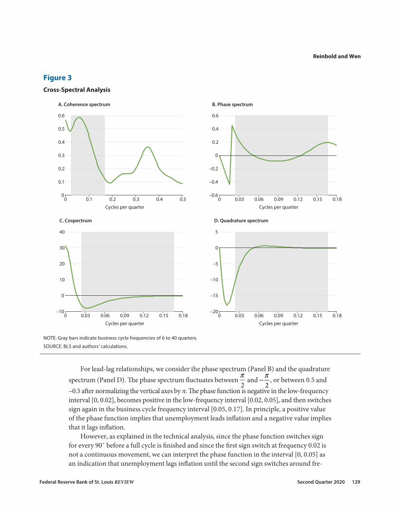
Next, we investigate the relationships between unemployment and inflation in the fre-quency domain. In Figure 3, Panel A plots the coherence function, which is analogous to the
−10
−5
0
5
10
15
19481953
19581963
19681973
19781983
19881993
19982003
20082013
2018
In�ation rateUnemployment rate
3 4 5 6 7 8 9 10
Unemployment rate (percent)
In�ation rate (percent)
1948:Q1 − 1969:Q41970:Q1 − 2018:Q4
Percent
−10
−5
0
5
10
15
A. Full sample B. Two subsamples
Figure 1Unemployment Rate and Inflation Rate
SOURCE: BLS and authors’ calculations.
Reinbold and Wen
128 Second Quarter 2020 Federal Reserve Bank of St. Louis REVIEW
absolute value of the correlation in the time domain. At low and business cycle frequencies, the two series are strongly correlated (with peak correlations of 0.57 at frequency zero and frequency 0.05, respectively, which each correspond to a long-run trend and periodicity of 20 quarters per cycle, respectively). Such strong correlations are completely missed by the time- domain plots in Panel A of Figure 1. The reason is that too much noise exists in the time domain and masks any systematic relationships. Indeed, the coherence function shows that at high frequencies, the coherence is mostly near zero except for a local peak at frequency 0.35. Hence, the coherence function suggests that the two seemingly uncorrelated time series (when viewed in the time domain) are actually strongly correlated at low and business cycle frequencies. But the noise at high frequencies (especially in the inflation rate) has masked such strong relationships.
However, note that the coherence does not give us any information on the sign of the correlation or the lead-lag relationships between the two variables. Hence, we need to explore the spectral information further. To highlight the details, we have truncated the spectral functions for frequencies higher than 0.18 in Panels B-D of Figure 3.
The cospectrum that captures the covariance between unemployment and inflation across cyclical frequencies is shown in Panel C. It suggests that the two variables are positively cor-related in the very long run (for frequencies lower than 0.02). However, they are negatively correlated at frequencies above 0.02 and have a trough at around 30 quarters per cycle. Their covariance becomes very small for frequencies higher than the conventional business cycle frequency interval (i.e., ω ≥ 1/6).
0 0.1 0.2 0.3 0.4 0.5
Cycles per quarter
0
0.02
0.04
0.06
0.08
0.10
0.12
0.14
A. Unemployment
0 0.1 0.2 0.3 0.4 0.5
Cycles per quarter
0
0.01
0.02
0.03
0.04
0.05
0.06
0.07
0.08
B. In�ation
Figure 2Power Spectrum of the Unemployment Rate and Inflation Rate
NOTE: Gray bars indicate business cycle frequencies of 6 to 40 quarters.
SOURCE: BLS and authors’ calculations.
Federal Reserve Bank of St. Louis REVIEW Second Quarter 2020 129
Reinbold and Wen
For lead-lag relationships, we consider the phase spectrum (Panel B) and the quadrature spectrum (Panel D). The phase spectrum fluctuates between
π2
and −π2
, or between 0.5 and –0.5 after normalizing the vertical axes by π. The phase function is negative in the low- frequency interval [0, 0.02], becomes positive in the low-frequency interval [0.02, 0.05], and then switches sign again in the business cycle frequency interval [0.05, 0.17]. In principle, a positive value of the phase function implies that unemployment leads inflation and a negative value implies that it lags inflation.
However, as explained in the technical analysis, since the phase function switches sign for every 90˚ before a full cycle is finished and since the first sign switch at frequency 0.02 is not a continuous movement, we can interpret the phase function in the interval [0, 0.05] as an indication that unemployment lags inflation until the second sign switches around fre-
0 0.1 0.2 0.3 0.4 0.5
Cycles per quarter
0
0.1
0.2
0.3
0.4
0.5
0.6
A. Coherence spectrum
0 0.03 0.06 0.09 0.12 0.15 0.18
Cycles per quarter
–0.6
–0.4
–0.2
0
0.2
0.4
0.6
B. Phase spectrum
0 0.03 0.06 0.09 0.12 0.15 0.18
Cycles per quarter
–10
0
10
20
30
40
C. Cospectrum
0 0.03 0.06 0.09 0.12 0.15 0.18
Cycles per quarter
–20
–15
–10
–5
0
5
D. Quadrature spectrum
Figure 3Cross-Spectral Analysis
NOTE: Gray bars indicate business cycle frequencies of 6 to 40 quarters.
SOURCE: BLS and authors’ calculations.
Reinbold and Wen
130 Second Quarter 2020 Federal Reserve Bank of St. Louis REVIEW
quency 0.05. That is, for low-frequency movements (with periodicity longer than 20 quarters per cycle), unemployment lags inflation, but for business cycle frequencies in the interval [0.05, 0.125] (8 to 20 quarters per cycle), unemployment slightly leads inflation (although the maximum lead is only 0.1π, or 20˚, and is not very significant).
Panel D of Figure 3, the quadrature spectrum, shows that unemployment indeed lags the inflation rate in the frequency interval [0, 0.05] (20 up to infinite quarters per cycle). The lead-lag relation is slightly reversed but not significant in higher-frequency intervals such as the frequency interval [0.05, 0.125]. Thus, at low frequencies or in the very long run and part of the intermediate run, inflation significantly leads unemployment; at the shorter end of the intermediate run, inflation slightly lags unemployment, but the relationship is not signifi-cant; and in the high-frequency interval [0.17, 0.5] (not shown in Panels B-D), no significant lead-lag relationship exists between inflation and unemployment.
However, even though the quadrature spectrum in Panel D indicates that unemployment significantly lags inflation in the low-frequency interval [0, 0.05], which suggests that inflation “causes” unemployment at low frequencies, the cospectrum in Panel C shows that the sign of the cospectrum switches once from positive to negative in the middle of this low-frequency interval at around frequency 0.02 (50 quarters per cycle), suggesting that high inflation “causes” (leads to) high unemployment in the very long run (cycles longer than 50 quarters) but “causes” (leads to) low unemployment in frequency interval [0.02, 0.05] cycles per quarter (20 to 50 quarters per cycle).
To summarize, the Phillips curve is positively sloped in the very long run in frequency interval [0, 0.02] and negatively sloped in the low-frequency interval [0.02, 0.025]. At the conventional business cycle frequency interval [0.025, 0.17] (6 to 40 quarters per cycle), the cospectrum remains negative, suggesting that the Phillips curve is negatively sloped, although the lead-lag relationships change directions slightly, from inflation strongly leading unemploy-ment in frequency interval [0, 0.05] to weakly lagging unemployment in part of the business cycle frequency interval [0.05, 0.125].
4.3 Time-Domain Filtering
The cospectrum in Panel C of Figure 3 tells us how to design band-pass filters to extract cyclical fluctuations from unemployment and inflation in the time domain: We should specify three frequency bands, [0, 0.02], [0.02, 0.17], and [0.17, 0.5] (50 quarters to infinity, 6 to 50 quarters, and 2 to 6 quarters per cycle, respectively).4 We should then be able to find that the correlation between the filtered unemployment and inflation rates is strongly positive in the first frequency band, strongly negative in the second frequency band, and near zero in the third frequency band.
Notice that the second frequency band includes the conventional business cycle frequency interval of [0.025, 0.17] (6 to 40 quarters per cycle) and part of the low-frequency movements in the interval [0.02, 0.025] (40 to 50 quarters per cycle). Our findings from spectral analysis suggest that the conventional definition of the business cycle frequency interval [0.025, 0.17] may be too restrictive for analyzing the Phillips curve.
Indeed, these predictions are confirmed in the time domain, as shown in Figure 4. In particular, Panel A of Figure 4 shows the high-frequency components of the data obtained
Federal Reserve Bank of St. Louis REVIEW Second Quarter 2020 131
Reinbold and Wen
Correlation = −0.06
−6
−4
−2
0
2
4
6
1948 1958 1968 1978 1988 1998 2008 2018
A. Short-term components
Correlation = −0.45
−4
−2
0
2
4
6
1948 1958 1968 1978 1988 1998 2008 2018
B. Business cycle components
Correlation = 0.38
1
2
3
4
5
6
7
8
1948 1958 1968 1978 1988 1998 2008 2018
C. Long-term components
In�ation rate Unemployment ratePercent
Percent
Percent
Figure 4Band-Pass-Filtered Unemployment and Inflation Rates
SOURCE: BLS and authors’ calculations.
Reinbold and Wen
132 Second Quarter 2020 Federal Reserve Bank of St. Louis REVIEW
by applying a band-pass filter that isolates fluctuations in the third frequency band that cor-respond to cycles with periodicity between 2 and 6 quarters per cycle. At this high-frequency band, inflation is extremely volatile compared with unemployment and their correlation is essen-tially zero, with a correlation of –0.06 with a standard error of 0.062, which is not significant. This correlation is slightly positive before 1970 [0.10] and slightly negative after 1970 [–0.16].
Panel B shows time-domain movements in the second frequency band (which includes the conventional business cycle components of the series) obtained by applying a band-pass filter that isolates components in the frequency band that correspond to cycles with periodicity between 6 and 50 quarters per cycle. As the panel shows, as inflation rises, unemployment falls over the business cycle. The Phillips curve is also remarkably stable in this frequency band, with a correlation of –0.45 for the whole sample, –0.41 before 1970, and –0.47 after 1970. Interestingly, the unemployment rate and the inflation rate are actually more negatively cor-related post-1970, in contrast to the nonfiltered raw data where the Phillips curve reverses.
Panel C of Figure 4 shows the movements in unemployment and inflation at the low- frequency band of 50 to infinite quarters per cycle (which is the residual component after subtracting the movements from the first two frequency bands). Obvious change is evident in the correlation between the long-run components of inflation and unemployment around 1970. Pre-1970, there is a strong negative correlation of –0.53, but that reverses to 0.26 after 1970. The overall correlation is 0.38.
These results suggest that the Phillips curve is alive and well over the intermediate run (including the conventional business cycle frequency interval) but that short-run irregularities and the long-run positive correlation have masked the Phillips curve relation in the time domain in the raw data. The low-frequency movements post-1970 have especially flattened the Phillips curve.
4.4 Shock Decomposition
The VAR-based spectral analysis of unemployment and inflation can be exploited further in both the frequency domain and the time domain. For example, the spectral density of both unemployment and inflation have a spectral peak at frequency zero. Using the shock-identi-fication method in the frequency domain proposed by Wen (2001, 2002), we conduct a struc-tural analysis in the frequency domain to decompose the spectrum (or cross spectrum) into two orthogonal components: (i) a spectrum (or cross spectrum) generated from a long-run shock that is responsible for the peak spectrum of unemployment at frequency zero (or in a frequency band near zero) and (ii) a spectrum (or cross spectrum) generated from an orthogonal shock that is not responsible for movements of unemployment at very low frequencies.
As explained by Wen (2001, 2002), the time domain analog of this frequency-domain decomposition is the method of Blanchard and Quah (1989), but Wen’s spectral decomposi-tion method is far more general since it can be applied in the frequency domain to any fre-quencies or frequency intervals. Also, it can be applied to either the power spectrum or the cross spectrum (cospectrum or quadrature spectrum) or any combination of them, whereas the method of Blanchard and Quah (1989) is only a special case of Wen’s generalized shock- identification method in the frequency domain. Wen’s generalized spectral method is useful
Federal Reserve Bank of St. Louis REVIEW Second Quarter 2020 133
here because we can use it to find structural shocks responsible for the existence and stability of the Phillips curve.
We now apply the method of Wen (2001, 2002) to the spectrum (or cross spectrum) of unemployment and inflation. In particular, for the sake of demonstration, we simply assume that two orthogonal structural shocks are responsible for the movements in unemployment and inflation, as in the spirit of Blanchard and Quah (1989) in the traditional structural VAR literature. One shock is called the “permanent shock,” and the other is called the “nonperma-nent shock,” and intuitively we can think of the permanent shock as a “supply” shock and the nonpermanent shock as a “demand” shock. The permanent shock is assumed to be responsible for the peak spectrum of unemployment at frequency zero, and the nonpermanent shock is assumed to be not responsible for this movement. Notice that these identifying assumptions do not impose any restrictions regarding how much the first and second shocks influence the spectrum of unemployment at nonzero frequencies—or how these two shocks influence the spectrum of inflation or the cross spectrum at any frequencies (including frequency zero). Instead, based on the limited identifying assumption, we let the data tell us how these two identified shocks determine the joint behaviors of unemployment and inflation in the frequency domain.
Once the structural identification and spectral decomposition are achieved in the frequency domain, the results can be easily converted to the time domain through the inverse Fourier transform, as the following exercises show.
Figure 5 demonstrates the structural decomposition of the spectrum and cospectrum under our simple identifying assumptions in the spirit of Blanchard and Quah (1989). Panel A shows the power spectrum of unemployment and its structural decomposition, where the blue solid line is the data power spectrum of unemployment, the red-dashed line is the con-tribution of the permanent shock to the spectrum of unemployment, and the green-dashed line is the contribution of the nonpermanent shock to the spectrum of unemployment. The identifying assumption is that the permanent shock explains the maximum amount of the power spectrum of unemployment at frequency zero, while the other shock explains the mini-mum, but no further assumptions or restrictions are made regarding their respective contri-butions to unemployment at nonzero frequencies or their contributions to inflation at any frequency (including frequency zero). As proved by Wen (2001, 2002), the identification is unique, so these two shocks’ contributions add up to the total spectral densities at each fre-quency between 0 and π. This panel shows that the permanent shock is largely responsible for the bulk of movements in unemployment at low frequencies, but its contribution declines toward higher frequencies, while the nonpermanent shock is largely responsible for the movements at the conventional business cycle frequency and high-frequency intervals.
However, with respect to inflation, Panel B shows that the two shocks split the data spec-trum (blue line) almost evenly across frequencies, or each shock contributes to about half of the power spectrum, with the permanent shock slightly dominating the nonpermanent shock at frequency zero.
The most interesting results are with respect to the cross spectrums shown in Panels C and D. Panel C shows that the data cospectrum (blue solid line) switches signs from positive
Reinbold and Wen
Reinbold and Wen
134 Second Quarter 2020 Federal Reserve Bank of St. Louis REVIEW
to negative at frequency 0.02. The structural decomposition reveals this switching occurs because of the contributions of the nonpermanent shock (green-dashed line), which generate negative covariance between unemployment and inflation across all frequencies, thus is essen-tially 100 percent responsible for the existence of the Phillips curve. In other words, without the nonpermanent shock, there would be no Phillips curve, since the permanent shock alone would have generated the cospectrum (red-dashed line), which is positive across the entire frequency domain.
Panel D shows the quadrature spectrum that reflects the lead-lag relationships between unemployment and inflation. It reveals that the permanent shock (red-dashed line) is entirely responsible for the negative part of the quadrature spectrum, so that unemployment lags
Figure 5Spectral Decomposition of Unemployment and Inflation
NOTE: Gray bars indicate business cycle frequencies of 6 to 40 quarters.
SOURCE: BLS and authors’ calculations.
Reinbold and Wen
Federal Reserve Bank of St. Louis REVIEW Second Quarter 2020 135
inflation significantly under this shock, which explains the effects of the two major oil shocks in the 1970s and early 1980s, during which high inflation caused by high oil prices generated high unemployment and stagnation in the U.S. economy. The nonpermanent shock (green-dashed line), however, is responsible for the slightly positive quadrature spectrum in the data (blue solid line) because under this type of shocks there is a sign switch near frequency 0.03, suggesting that under a nonpermanent shock, unemployment tends to lag inflation only at frequencies below 0.03 but tends to lead inflation at frequencies above 0.03.
These findings have important monetary policy implications. If monetary policy mainly affects nonpermanent shocks or the demand side of the economy, then policymakers may be able to use high-inflation policy to lower unemployment in the long-run frequency interval [0.00, 0.03], which does not include much of the conventional business cycle frequency interval [0.025, 0.17]. In the conventional business cycle frequency interval, inflation lags unemploy-ment instead, so monetary policy does not “cause” unemployment through inflation targeting, although such a “causal” effect is not very strong based on quarterly data.
Since the spectrum and cospectrum are moment-generating functions and they contain information about autocovariance and cross variance of a vector of time series at any leads and lags, the above structural decomposition can be converted back to the time domain by applying the inverse Fourier transform.
Figure 6 shows the impulse response functions of unemployment and inflation under the permanent and nonpermanent shocks, respectively, identified in the frequency domain. Panel A shows that unemployment (green solid line) and inflation (red-dashed line) move in
0 5 10 15 20 25 30 35 40
Time
–0.6
–0.4
–0.2
0
0.2
0.4
0.6
0.8
1.0
1.2
A. Response to nonpermanent shock
0 5 10 15 20 25 30 35 40
Time
–0.2
0
0.2
0.4
0.6
0.8
1.0
1.2
1.4
1.6
1.8
B. Response to permanent shock
UnemploymentIn�ation
Figure 6Impulse Response Function of Unemployment and Inflation Under Structural Shocks
SOURCE: BLS and authors’ calculations.
Reinbold and Wen
136 Second Quarter 2020 Federal Reserve Bank of St. Louis REVIEW
opposite directions under a one-standard-deviation nonpermanent shock, and both series are highly persistent. Panel B shows that unemployment and inflation move together under a permanent shock because both respond positively to the shock.
Next, we simulate time series based on the uncovered autocoefficients from the inverse Fourier transform and the two identified structural shocks (using information from the residuals of the VAR in the time domain upon which the Fourier transform is based). The uncovered time series under each structural shock process and their relationships are presented in Figure 7.
Panel A of Figure 7 shows the raw unemployment data (vertical axis) against the raw infla-
–15 –10 –5 0 5 10 15
In�ation (percent)
–4
–2
0
2
4
6Unemployment (percent)
A. Raw Data: Beta = 0.03
–8 –6 –4 –2 0 2 4 6 8
In�ation (percent)
–3
–2
–1
0
1
2
3
B. Permanent Shock: Beta = 0.33
–8 –6 –4 –2 0 2 4 6 8
In�ation (percent)
–3
–2
–1
0
1
2
3
4
C. Nonpermanent Shock: Beta = –0.35
–15 –10 –5 0 5 10 15
In�ation (percent)
–4
–2
0
2
4
6
D. Both Shocks: Beta = 0.03
Unemployment (percent)
Unemployment (percent) Unemployment (percent)
Figure 7Unemployment vs. Inflation under Permanent and Nonpermanent Shocks
SOURCE: BLS and authors’ calculations.
Reinbold and Wen
Federal Reserve Bank of St. Louis REVIEW Second Quarter 2020 137
tion data (horizontal axis). The straight regression line shows that the slope is weakly positive, with a value of 0.03, which is not statistically different from zero. Hence, according to this panel, the Phillips curve does not exist, as the literature often claims.
Panel B shows the same two time series but under only the permanent shock. The regression line has a strong, positive slope, with a value of 0.33, which is highly statistically significant. Hence, according to this panel, the Phillips curve is turned on its head under a permanent shock.
Panel C shows the same two time series under only the nonpermanent shock. The regres-sion line is negatively sloped, with a value of –0.35, which is highly statistically significant. Hence, according to this panel, the Phillips curve definitely exists under a nonpermanent shock.
Finally, Panel D mixes the decomposed time series together under both shocks and then plots the mixed unemployment series against the mixed inflation series. It shows the same result as Panel A based on the raw data—namely, the Phillips curve disappears.
These results suggest that the very reason that the literature cannot find the existence of the Phillips curve is simply because permanent and nonpermanent shocks lead to the opposite slopes of the Phillips relationship, so the true Phillips curve is masked by permanent shocks in the time domain, as our structural analyses clearly reveals.
5 CONCLUSIONWe employ spectral techniques to analyze the U.S. Phillips curve in the frequency domain.
We find that (i) the Phillips curve is strongly positively sloped at the low-frequency interval [0, 0.02] (50 or more quarters per cycle) and (ii) the Phillips curve has the correct negative slope in the frequency interval [0.02, 0.17] (6 to 50 quarters per cycle), which includes the conventional business cycle of 6 to 40 quarters and a portion of the low-frequency interval. The negative relationship is also stable over time despite the oil shocks during the 1970s. There do not exist systemic relationships between the two series at frequencies higher than 0.17 (6 quarters or less per cycle).
We use our spectral analysis as a guide for specifying the windows for band-pass filters. Again, we find that there is a negative and stable Phillips curve at the business cycle frequency. We conclude that short-run fluctuations and long-term trend components of the data mask the Phillips curve in the data.
The phase spectrum analysis shows that despite the existence of the Phillips curve at the business cycle frequency, the monetary policy implications are not obvious. In order for mone-tary policy to be effective in exploiting the trade-off between inflation and unemployment, it would be best for inflation to lead unemployment, so that a policy-induced increase in the inflation rate can lead to lower unemployment. However, we cannot find systematic and sig-nificant lead-lag relationships in the quadrature spectrum between unemployment and infla-tion at frequency intervals that monetary policy could exploit. If anything, unemployment weakly leads inflation, or inflation weakly lags unemployment, at the conventional business cycle frequency. This finding casts doubt on the so-called tradeoff between unemployment and inflation even if the Phillips curve is negatively sloped.
Reinbold and Wen
138 Second Quarter 2020 Federal Reserve Bank of St. Louis REVIEW
We also use the generalized structural identification method of Wen (2001, 2002) in the frequency domain to identify two structural shocks: a permanent shock that causes long-run movements in unemployment at frequency zero and a nonpermanent shock that is orthogo-nal to the permanent shock. We reveal that nonpermanent shocks are responsible for almost the entire negative relationship between unemployment and inflation in the frequency interval [0.02, 0.17], while the positive relationship in the frequency interval [0, 0.02] is entirely due to the permanent shock. We also illustrate the time-series properties of the two shocks and their implied movements in unemployment and inflation in the time domain, using the inverse Fourier transform. We show that in the time domain, permanent shock-implied movements and nonpermanent shock-implied movements in unemployment and inflation move in oppo-site directions and lead to a mixture that masks any significant and systemic relationships between unemployment and inflation. In addition, when we split the sample into two sub-samples, we obtain the same results. So the policy implication is that for monetary policy to be at all effective in exploiting the trade-off between inflation and unemployment, it must be conducted only under nonpermanent shocks and not under permanent shocks (such as the oil shocks). In fact, it may be counterproductive under permanent shocks.
We conclude that the Phillips curve is alive and well, at least at the business cycle frequency and under nonpermanent shocks (which are often interpreted as demand-side shocks). How-ever, short-term changes in the inflation rate will not necessarily lead to immediate changes in the unemployment rate. Instead, it is important to look at the intermediate run. In the long run, inflation leads to high unemployment instead of low unemployment. n
Reinbold and Wen
Federal Reserve Bank of St. Louis REVIEW Second Quarter 2020 139
APPENDIX 1: A BRIEF TECHNICAL REVIEW OF SPECTRAL ANALYSIS
Given a square-summable sequence cn{ }n=−∞∞
n=−∞
∞
∑ cn2⎛
⎝⎜⎞⎠⎟<∞ , its Fourier transform is
defined as
f ω( )=j=−∞
∞
∑ c je−iω j ,
where ω [–π,π] is angular frequency, i ≡ −1 is the imaginary unit, and e±ix = cos(x) ± isin(x) is the Fourier operator. Given the function f(ω), each element ck in the original sequence {cn}∞
n=–∞ can be recovered from the inverse Fourier transform:
ck = 12π −π
π
∫ f ω( )e+iωkdω .
To apply the Fourier technique to time-series analysis, consider a white-noise process et with mean zero and variance σ2
e. Based on the white-noise process, we can construct a new time series:
yt =j=0
∞
∑bjet− j = B L( )et ,
where L is the lag operator. The covariogram (autocovariance) at any lag τ (–∞,∞) of this new time series is given by
cy τ( )= Eyt yt−τ =σ e2
j= −∞
∞
∑ bjbj−τ Note:bj = 0 for j <τ( ).Applying the Fourier transform to the sequence {cy(τ)}∞
τ=–∞ gives the power spectrum (or spectral density function) of yt:
g y e−iω( )=τ=−∞
∞
∑ cy τ( )e−iωτ = B e−iω( )B eiω( )σ e2 .
There are several basic properties of the spectral density function over the domain ω [–π,π]: (i) It is real valued and nonnegative; (ii) it is symmetric about ω = 0, or gy(e–iω) = gy(eiω); and (iii) a spectral peak (local maximum) at ω0 reflects relatively large contributions from cyclical fluctuations of around 2π/ω0 periods per cycle.
Using the inverse Fourier transform, we can recover the autocovariance at any lead or lag τ (–∞,∞):
cy τ( )= 1
2π −π
π
∫ g y e−iω( )e+iωτdω
cy 0( )= 12π −π
π
∫ g y e−iω( )dω ,
where cy(0) is the variance of the original time series. That is, the spectrum gy(e–iω) is a moment- generating function and the total area underneath the spectrum is proportional (2π times) to the total variance of yt. It is in this sense that we view the spectrum as a distribution of variance across cyclical frequencies.
Reinbold and Wen
140 Second Quarter 2020 Federal Reserve Bank of St. Louis REVIEW
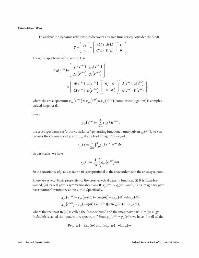
To analyze the dynamic relationships between any two time series, consider the VAR
Yt =ytxt
⎛
⎝⎜⎜
⎞
⎠⎟⎟=
A L( ) B L( )C L( ) D L( )
⎛
⎝⎜⎜
⎞
⎠⎟⎟
et
µt
⎛
⎝⎜⎜
⎞
⎠⎟⎟.
Then, the spectrum of the vector Yt is
≡ g e−iω( )=g y e−iω( ) g yx e−iω( )gxy e−iω( ) gx e−iω( )
⎛
⎝
⎜⎜
⎞
⎠
⎟⎟
= A e−iω( ) B e−iω( )C e−iω( ) D e−iω( )
⎛
⎝
⎜⎜
⎞
⎠
⎟⎟
σ e2 0
0 σ µ2
⎛
⎝⎜⎜
⎞
⎠⎟⎟
A eiω( ) B eiω( )C eiω( ) D eiω( )
⎛
⎝
⎜⎜
⎞
⎠
⎟⎟ ,
where the cross spectrum g yx e−iω( )= gxy eiω( )≡ gxy e−iω( ) (complex conjugation) is complex- valued in general.
Since
g yx e−iω( )≡τ=−∞
∞
∑ cyx k( )e−iωτ ,
the cross spectrum is a “cross-covariance” generating function; namely, given gyx(e–iω), we can recover the covariance of yt and xt–τ at any lead or lag τ (–∞,∞):
cyx τ( )= 12π
g yx−π
π∫ e−iω( )eiωτdω .
In particular, we have
cyx 0( )= 12π −π
π
∫ g yx e−iω( )dω .
So the covariance of yt and xt (at τ = 0) is proportional to the area underneath the cross spectrum.
There are several basic properties of the cross-spectral density function: (i) It is complex- valued; (ii) its real part is symmetric about ω = 0: gy(e–iω) = gy(eiω); and (iii) its imaginary part has rotational symmetry about ω = 0. Specifically,
g yx e−iω( )= g yx cos ω( )− isin ω( )( )≡Re yx ω( )− iIm yx ω( )gxy e+iω( )= gxy cos ω( )+ isin ω( )( )≡Rexy ω( )+ iImxy ω( ),
where the real part Re(ω) is called the “cospectrum” and the imaginary part ±Im(ω) (sign included) is called the “quadrature spectrum.” Since gyx(e–iω) = gxy(eiω), we have (for all ω) that
Re yx ω( )= Rexy ω( ) and Im yx ω( )= −Imxy ω( ).
Reinbold and Wen
Federal Reserve Bank of St. Louis REVIEW Second Quarter 2020 141
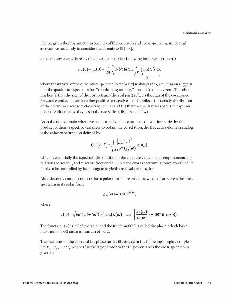
Hence, given these symmetry properties of the spectrum and cross spectrum, in spectral analysis we need only to consider the domain ω [0,π].
Since the covariance is real valued, we also have the following important property:
cyx 0( )= cxy 0( )= 12π −π
π
∫Re ω( )dω ± i2π −π
π
∫ Im ω( )dω
=01 244 344
,
where the integral of the quadrature spectrum over [–π,π] is always zero, which again suggests that the quadrature spectrum has “rotational symmetry” around frequency zero. This also implies (i) that the sign of the cospectrum (the real part) reflects the sign of the covariance between yt and xt—it can be either positive or negative—and it reflects the density distribution of the covariance across cyclical frequencies and (ii) that the quadrature spectrum captures the phase differences of cycles in the two series (discussed below).
As in the time domain where we can normalize the covariance of two time series by the product of their respective variances to obtain the correlation, the frequency-domain analog is the coherence function defined by
Coh e−iω( )≡ g yx ω( )2
g y ω( )gx ω( ) ∈ 0,1[ ],
which is essentially the (spectral) distribution of the absolute value of contemporaneous cor-relations between yt and xt across frequencies. Since the cross spectrum is complex-valued, it needs to be multiplied by its conjugate to yield a real-valued function.
Also, since any complex number has a polar form representation, we can also express the cross spectrum in its polar form:
g yx ω( )= r ω( )eiθ ω( ) ,
where
r ω( )= Re2 ω( )+ Im2 ω( ) and θ ω( )= tan−1 qu ω( )co ω( )
⎡
⎣⎢
⎤
⎦⎥ +180° if co < 0( ).
The function r(ω) is called the gain, and the function θ(ω) is called the phase, which has a maximum of π/2 and a minimum of –π/2.
The meanings of the gain and the phase can be illustrated in the following simple example: Let Yt = xt–k = Lkxt, where Lk is the lag operator to the kth power. Then the cross spectrum is given by
Reinbold and Wen
142 Second Quarter 2020 Federal Reserve Bank of St. Louis REVIEW
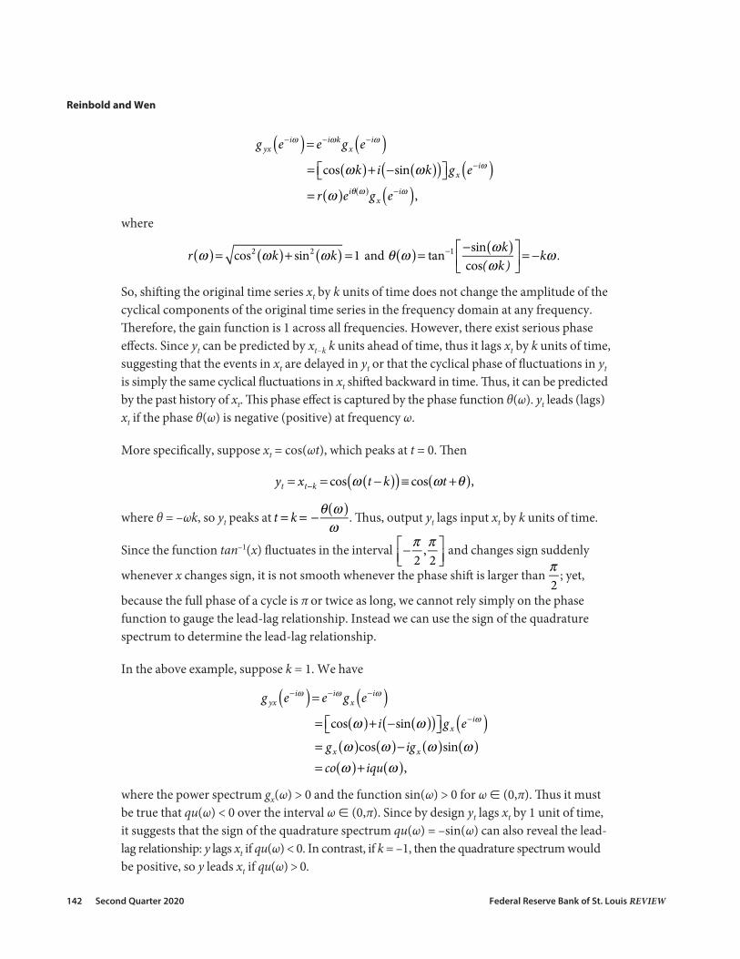
g yx e−iω( )= e−iωk gx e−iω( )= cos ωk( )+ i −sin ωk( )( )⎡⎣ ⎤⎦ gx e−iω( )= r ω( )eiθ ω( )gx e−iω( ),
where
r ω( )= cos2 ωk( )+ sin2 ωk( ) =1 and θ ω( )= tan−1 −sin ωk( )cos(ωk)
⎡⎣⎢
⎤⎦⎥= −kω .
So, shifting the original time series xt by k units of time does not change the amplitude of the cyclical components of the original time series in the frequency domain at any frequency. Therefore, the gain function is 1 across all frequencies. However, there exist serious phase effects. Since yt can be predicted by xt–k k units ahead of time, thus it lags xt by k units of time, suggesting that the events in xt are delayed in yt or that the cyclical phase of fluctuations in yt is simply the same cyclical fluctuations in xt shifted backward in time. Thus, it can be predicted by the past history of xt. This phase effect is captured by the phase function θ(ω). yt leads (lags) xt if the phase θ(ω) is negative (positive) at frequency ω.
More specifically, suppose xt = cos(ωt), which peaks at t = 0. Then
yt = xt−k = cos ω t − k( )( )≡ cos ωt +θ( ),
where θ = –ωk, so yt peaks at t = k = −θ ω( )ω
. Thus, output yt lags input xt by k units of time.
Since the function tan–1(x) fluctuates in the interval −π2,π2
⎡⎣⎢
⎤⎦⎥
and changes sign suddenly
whenever x changes sign, it is not smooth whenever the phase shift is larger than π2
; yet,
because the full phase of a cycle is π or twice as long, we cannot rely simply on the phase function to gauge the lead-lag relationship. Instead we can use the sign of the quadrature spectrum to determine the lead-lag relationship.
In the above example, suppose k = 1. We have
g yx e−iω( )= e−iω gx e−iω( )= cos ω( )+ i −sin ω( )( )⎡⎣ ⎤⎦ gx e−iω( )= gx ω( )cos ω( )− igx ω( )sin ω( )= co ω( )+ iqu ω( ),
where the power spectrum gx(ω) > 0 and the function sin(ω) > 0 for ω (0,π). Thus it must be true that qu(ω) < 0 over the interval ω (0,π). Since by design yt lags xt by 1 unit of time, it suggests that the sign of the quadrature spectrum qu(ω) = –sin(ω) can also reveal the lead-lag relationship: y lags xt if qu(ω) < 0. In contrast, if k = –1, then the quadrature spectrum would be positive, so y leads xt if qu(ω) > 0.
Reinbold and Wen
Federal Reserve Bank of St. Louis REVIEW Second Quarter 2020 143
In contrast, the phase spectrum shows that
θ ω( )= tan−1 −sin ω( )cos ω( )
⎡
⎣⎢
⎤
⎦⎥ =
−ω if ω ∈ 0,π / 2[ ]ω if ω ∈ π / 2,π[ ]
⎧⎨⎪
⎩⎪
⎫⎬⎪
⎭⎪,
where we know that when ω ∈ π2,π⎛
⎝⎜⎞⎠⎟ , cos θ( )< 0, so θ ω( )> 0; thus, the phase spectrum
suggests that yt leads xt once ω > π2
, which cannot be right since by design yt lags xt. Hence,
caution must be exercised when using the phase function to gauge lead-lag relations. The reason is as follows: For pure sin waves, a lead can also be interpreted as a lag if the lead is too big (larger than half the length of the full cycle or 180˚in phase angle). Since the phase function
switches sign for every 90˚ or π2
, it is better to use the sign of the quadrature spectrum to gauge the lead-lag relationship.
APPENDIX 2: UNIT ROOT TEST
The augmented Dickey-Fuller test fits a model of the form
Δyt =α +β yt−1 +j=1
p
∑φ jΔyt− j +et ,
where y is the variable under consideration and p is the maximum number of lags (we set p = 4). The null hypothesis is β = 0, or, equivalently, that yt follows a unit process. From Table A2.1, we reject the null hypothesis at the 1 percent level for the inflation rate and at the 5 percent level for the unemployment rate. Therefore, we can conclude that the inflation rate and the unemployment rate are stationary.
Table A2.1Unit Root Test
t-Statistic p-Value
Inflation rate –3.683 0.004
Unemployment rate –2.936 0.041
Reinbold and Wen
144 Second Quarter 2020 Federal Reserve Bank of St. Louis REVIEW
NOTES1 Phillips’s original analysis was based on the wage inflation rate, but later research replaced the wage inflation
rate simply with the general price inflation rate.
2 We define the conventional business cycle frequency as fluctuations between 6 and 40 quarters per cycle.
3 We find that four lags in the VAR are optimal, and our results are robust to other lag specifications.
4 We use the Baxter-King (1999) approximation to the band-pass filter. Baxter and King (1999) derived their method for nonstationary time series by imposing that the filter coefficients sum to zero. Dropping this condition yields a filter for stationary time series. We assume that the inflation rate and unemployment rate are stationary, and we verify this assumption by running Dickey-Fuller tests. See the appendix.
REFERENCESBaxter, Marianne and King, Robert G. “Measuring Business Cycles: Approximate Band-Pass Filters for Economic
Time Series.” Review of Economics and Statistics, 1999, 81(4), pp. 575-93; https://doi.org/10.1162/003465399558454.
Blanchard, Olivier Jean and Quah, Danny. “The Dynamic Effects of Aggregate Demand and Supply Disturbances.” American Economic Review, 1989, 79(4) pp. 655-73; https://www.jstor.org/stable/1827924.
Gallegati, Marco; Gallegati, Mauro; Ramsey, James Bernard and Semmler, Willi. “The US Wage Phillips Curve across Frequencies and over Time.” Oxford Bulletin of Economics and Statistics, 2011, 73(4), pp. 489-508; https://doi.org/10.1111/j.1468-0084.2010.00624.x.
Gordon, Robert J. “The History of the Phillips Curve: Consensus and Bifurcation.” Economica, 2011, 78, pp. 10-50; https://doi.org/10.1111/j.1468-0335.2009.00815.x.
Iacobucci, Alessandra. “Spectral Analysis for Economic Time Series,” in Jacek Leskow, Lionello F. Punzo, and Martin Puchet Anyul, eds., New Tools for Economic Dynamics. Lecture Notes in Economics and Mathematical Systems. Volume 551. Springer, 2005, pp. 203-19; https://doi.org/10.1007/3-540-28444-3_12.
King, Robert G. and Watson, Mark W. “The Post-War U.S. Phillips Curve: A Revisionist Econometric History.” Carnegie-Rochester Conference Series on Public Policy, 1994, 41, pp. 157-219; https://doi.org/10.1016/0167-2231(94)00018-2.
Phillips, A.W. “The Relation Between Unemployment and the Rate of Change of Money Wage Rates in the United Kingdom, 1861-1957.” Economica, 1958, 25(100), pp. 283-99; https://doi.org/10.2307/2550759.
Samuelson, Paul A. and Solow, Robert M. “Analytical Aspects of Anti-Inflation Policy.” American Economic Review, 1960, 50(2), pp. 177-94.
Scully, Gerald W. “Static vs. Dynamic Phillips Curves.” Review of Economics and Statistics, 1974, 56(3), pp. 387-90; https://doi.org/10.2307/1923978.
Wen, Yi. “A Generalized Method of Impulse Identification.” Economics Letters, 2001, 73(3), pp. 367-74; https://doi.org/10.1016/S0165-1765(01)00509-2.
Wen, Yi. “The Business Cycle Effects of Christmas.” Journal of Monetary Economics, 2002, 49(6), pp. 1289-314; https://doi.org/10.1016/S0304-3932(02)00150-2.