Is there an Almeida-Thouless line in Spin Glasses? Peter Young e-mail:[email protected]Work supported by the Collaborator: H. G. Katzgraber Talk at the APS March Meeting, New Orleans, March 11, 2008 This talk can be downloaded at http://www.physics.ucsc.edu/˜peter/talks/APS2008.pdf – p.1
They proposed that the exact solution be the mean field theory of spinglasses.
It was hoped that the solution would be:
• simple
• a reasonable approximation to real spin glasses
To what extent are these hopes realized?
– p.3
Is the SK model simple?
The SK solution (replica-symmetric solution) is simple.
However SK realized that it cannot be correct at low temperature (negativeentropy).
Situation clarified by Almeida and Thouless (1978). In a magnetic field,the replica-symmetric solution is unstable below a line in the H-T plane(the AT line).
Tc
H
T0
AT line
RS solution(simple)
RSB solution
(complicated)(Parisi)
Below the AT line the exactsolution, which is complicated ,was found in a tour-de-forceby Parisi (replica symmetrybreaking).The Parisi solution was sub-sequently found to be:
• stable (de Dominicis andKondor)
• exact (Tallegrand)– p.4
Parisi SolutionThe Parisi (RSB) solution has two important features:
• There is a transition in a field (AT line), as we have seen.
• The order parameter is not just a single number but a whole function.Defining the spin overlap by
q =1
N
N∑
i=1
S(1)i S
(2)i [(1)and (2) refer to 2 copies]
then q has a proba-bility distribution P (q)
(Parisi) which, for zerofield, looks like this:
Above the AT line P (q)is just a single deltafunction (the RS solu-tion).
P(q)
q
1−1
Do these features occur in real spin glasses, or are they artefacts of theinfinite-range SK model? – p.5
Is the SK model relevant?
Equilibrium state below TSG. Two main scenarios:
“Replica Symmetry Breaking”(RSB), (Parisi).
Assume short-range is similarto the infinite-range SK model.
• P (q) is non-trivial.
• There is an AT line.
“Droplet picture” (DP) (Fisher andHuse, also Bray and Moore, andMcMillan).
Focus on the geometrical aspectsof the low-energy excitations.
• P (q) is trivial (for L → ∞).
• There is no AT line.
– p.6
ModelsWe perform Monte Carlo simulations on the following models:
• Nearest-neighbor model in d = 3.No. of spins is N = L3, where L is not very big (even with paralleltempering to help speed things up.)Would also like to do higher-d. But there the range of L is evensmaller. Hence we also study . . .
• Long-range model in d = 1.
Jij ∝ǫij
rσij
, [ǫij]av = 0, [ǫ2ij]av = 1 .
Can have a finite TSG for a range of σ (next slide).
When we apply a field we use a Gaussian distribution of random fields,[h2
i ] = H2r , rather than a uniform field. (Useful equilibration test.)
For the SK model, there is an AT line for Gaussian random fields, as for auniform field. (Note: the sign of the field can be “gauged away”.)
– p.7
Long-Range model in d = 1
Jij ∝ǫij
rσij
, [ǫij]av = 0, [ǫ2ij]av = 1 .
For the short-range model:
• there is a lower critical dimension dl (equal to about 2.5,
• and an upper critical dimension dl (equal to 6).
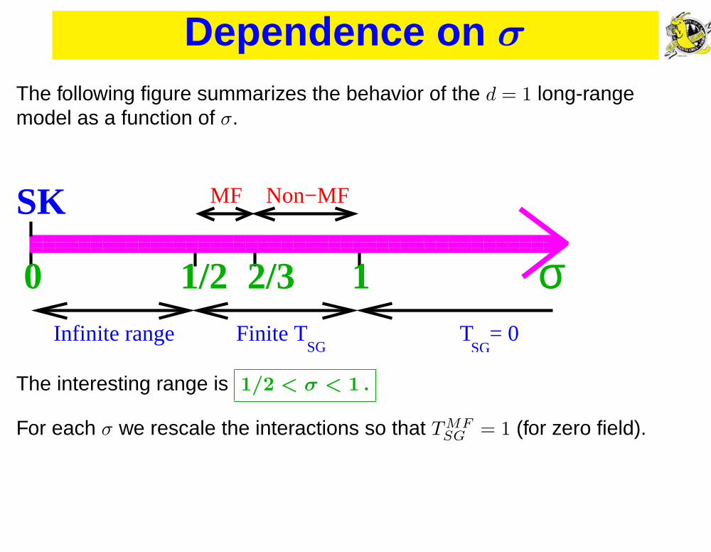
Make an analogy between varying d for short-range, and varying σ forlong-range d = 1. (Works for ferromagnets, e.g. Fisher, Ma and Nickel.)In otherwords there is a σl above which TSG = 0, and a σu below whichthe zero-field critical behavior is mean-field like, where
• σl = 1, (Fisher and Huse)
• σu = 2/3, (Kotliar, Stein and Anderson)
• Note too that σ = 0 is SK model
• The range 0 ≤ σ ≤ 1/2 is infinite-range since∑
j [J2
ij ]av diverges.
• σ → ∞ is the nearest-neighbor model.– p.8
Dependence on σ
The following figure summarizes the behavior of the d = 1 long-rangemodel as a function of σ.
For each σ we rescale the interactions so that TMFSG = 1 (for zero field).
– p.9
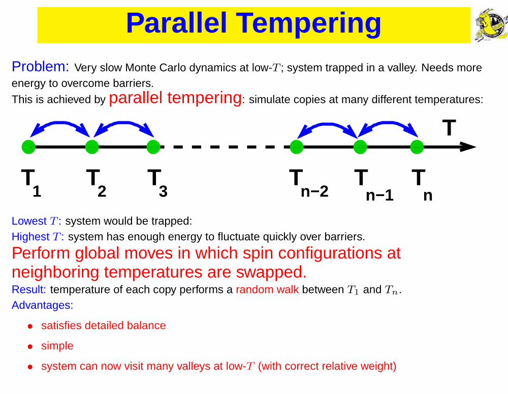
Parallel TemperingProblem: Very slow Monte Carlo dynamics at low-T ; system trapped in a valley. Needs moreenergy to overcome barriers.
This is achieved by parallel tempering: simulate copies at many different temperatures:
��������
��������
����
��������
��������
����
T
T
T T T1 2 n−1 n
T T3 n−2
Lowest T : system would be trapped:Highest T : system has enough energy to fluctuate quickly over barriers.
Perform global moves in which spin configurations atneighboring temperatures are swapped.Result: temperature of each copy performs a random walk between T1 and Tn.Advantages:
• satisfies detailed balance
• simple
• system can now visit many valleys at low-T (with correct relative weight)– p.10
Equilibration: 1For a Gaussian distribution of random bonds and fields, one can show (byintegrating by parts over the disorder distribution) that (for the short-rangecase)
[U ]av =z
2
J2
T([ql]av − 1) +
H2r
T([q]av − 1) ,
where U is the average energy,
ql =1
Nb
∑
〈i,j〉
〈SiSj〉2 is the “link overlap”
q =1
N
∑
i
〈S2
i 〉 is the “spin overlap” ,
z (= 6) is the lattice coordination number, and Nb = Nz/2.Note: This connection is for quantities that have been averaged overdisorder.
– p.11
Equilibration: 2
Equilibration test(Data for long range model.)As the number of sweeps in-creases, [U ]av monotonicallydecreases, while U(ql, q) mono-tonically increases, where
U(ql, q) =J2
T([ql]av − 1)+
H2
r
T([q]av − 1)
(J and ql generalized to thelong-range case). Once U =U(ql, q)
the results don’t change if thenumber of sweeps is increasedfurther.
From Katzgraber and APY, Phys. Rev. B, 72, 184416 (2005).– p.12
Correlation LengthWe will see that the most useful quantity for finite-size scaling is thecorrelation length of the finite system, ξL.To determine ξL first compute the spin glass correlation function at finitewavevector. In a non-zero magnetic field this involves the “connected”correlation function
χSG(k) =1
N
∑
i,j
[(〈SiSj〉 − 〈Si〉〈Sj〉)2]aveik·(Ri−Rj)
For zero field, where 〈Si〉 = 0, one has χSG(0) ∝ χnl, which can bemeasured experimentally. However, in a field χSG(0) is not related to χnl.Whereas χSG(0) diverges on the AT line (for the SK model) (it is the“replicon” mode), χnl does not. Hence there is
no static, experimentally measurable, divergent quantity on the AT line.
However, there is such a quantity, χSG(0), in the simulations .
We then determime ξL from the Ornstein Zernicke equation
χSG(k) =χSG(0)
1 + ξ2Lk2 + . . .
,
by fitting to k = 0 and k = kmin = (2π/L)(1, 0, 0). – p.13
Finite size scalingAssumption: size dependence comes from the ratio L/ξbulk where
ξbulk ∼ (T − TSG)−ν
is the bulk correlation length. (Note: (L/ξbulk)1/ν ∝ L1/ν(T − Tc).)
In particular, the finite-size correlation length varies as
ξL
L= X
(
L1/ν(T − TSG))
,
since ξL/L is dimensionless (and so has no power of L multiplying thescaling function X).
Hence data for ξL/L for different sizes should intersect at TSG and splayout below TSG.
Let’s first see how this works for the Ising SG in zero field, both for theshort-range d = 3 and long-range d = 1 models . . .
– p.14
Short-Range: Hr = 0
Crossings of the corre-lation length for the 3-d short-range Ising spinglass. Method first usedfor SG by Ballesteros etal., but for the ±J distribu-tion.
The clean intersections(corrections to FSS visiblefor L = 4) imply
TSG ≃ 0.96.
Prevously Marinari etal. found TSG = 0.95±0.04using a different analysis.
Katzgraber and APY (unpublished)– p.15
Long-Range: Hr = 0
A transition is observed in zero field for ALL these values of σ.H. G. Katzgraber and APY, Phys. Rev. B, 72, 184416 (2005). – p.16
Now do H 6= 0
Now we see now this procedure works for the case of non-zero field, againfor both the short-range d = 3 and long-range d = 1 models.According to RSB ξL diverges for L → ∞ on the AT line, so we look forintersections.
– p.17
Short-Range: Hr = 0.1
Crossings of the corre-lation length for the 3-d short-range Ising spinglass in a (Gaussian ran-dom) field of strengthHr = 0.1.
The lack of intersectionsimplies that there is no ATline down to this value ofHr.
Katzgraber and APY (unpublished and Phys. Rev. Lett. 93, 207203 (2004)).
– p.18
Long-Range: Hr = 0.1
A transition seems to be observed in a field for σ . 2/3.H. G. Katzgraber and APY, Phys. Rev. B, 72, 184416 (2005). – p.19
Summary
Does an AT line occur:
– p.20
Summary
Does an AT line occur:
1. only for the infinite-range (SK) model?
– p.20
Summary
Does an AT line occur:
1. only for the infinite-range (SK) model?
2. in real short-range three-dimensional spin glasses?
– p.20
Summary
Does an AT line occur:
1. only for the infinite-range (SK) model?
2. in real short-range three-dimensional spin glasses?
3. in short-range spin glasses for dimensions greater than a criticalvalue which is above 3?
– p.20
Summary
Does an AT line occur:
1. only for the infinite-range (SK) model?
2. in real short-range three-dimensional spin glasses?
3. in short-range spin glasses for dimensions greater than a criticalvalue which is above 3?
Based on Monte Carlo simulations (and using the analogy between theshort-range and long-range models) the answer seems to be 3.
There is an AT line above a critical dimension which seems to be dc = 6,the upper critical dimension for the zero field transition.