167
Xiaozhou Li 865007 789461 9 ISBN 9789461865007

Xiaozhou Li
8650077894619
ISBN 9789461865007
Smoothness-Increasing Accuracy-Conserving Filters forDiscontinuous Galerkin Methods: Challenging the
Assumptions of Symmetry and Uniformity
PROEFSCHRIFT
ter verkrijging van de graad van doctoraan de Technische Universiteit Delft,
op gezag van de Rector Magnificus prof.ir. K.C.A.M. Luyben,voorzitter van het College voor Promoties,
in het openbaar te verdedigen opdonderdag 9 juli 2015 om 10:00 uur
door
XIAOZHOU LI
Bachelor of Science, Mathematics and Applied Mathematics,University of Science and Technology of China, China
geboren te Chongqing, China
This dissertation has been approved by the
Promotor: Prof.dr.ir. C. VuikCopromotor: Dr. J.K. Ryan
Composition of the doctoral committee:
Rector Magnificus, voorzitterProf.dr.ir. C. Vuik, Technische Universiteit Delft, promotorDr. J.K. Ryan, University of East Anglia,
United Kingdom, copromotor
Independent members:
Prof.dr.ir. A.W. Heemink, Technische Universiteit DelftDr.ir. M.I. Gerritsma, Technische Universiteit DelftProf.dr.ir. J.E. Frank, Universiteit UtrechtProf.dr.ir. J.J.W. van der Vegt, Universiteit TwenteProf.dr. R.M. Kirby, University of Utah, United States
Smoothness-Increasing Accuracy-Conserving Filters for Discontinuous Galerkin Meth-ods: Challenging the Assumptions of Symmetry and Uniformity.
Dissertation at Delft University of Technology.
This research was carried out at Delft Institute of Applied Mathematics, Delft Uni-versity of Technology, and sponsored by the Air Force Office of Scientific Research(AFOSR), Air Force Material Command, USAF, under grant number FA8655-09-1-3017.
Copyright c© 2015 by Xiaozhou Li.
All rights reserved. No part of this publication may be reproduced or transmitted inany form or by any means, electronic or mechanical, including photocopy, recording,or any information storage and retrieval system, without permission in writing fromthe author.
ISBN 978-94-6186-500-7
Published by TU Delft Library.
Printed in the Netherlands by Ridderprint.

Summary
SIAC Filters: Challenging the Assumptions of Symmetryand Uniformity
In this dissertation, we focus on exploiting superconvergence for discontinuous Galerkinmethods and constructing a superconvergence extraction technique, in particular,Smoothness-Increasing Accuracy-Conserving (SIAC) filtering. The SIAC filtering tech-nique is based on the superconvergence property of discontinuous Galerkin methodsand aims to achieve a solution with higher accuracy order, reduced errors and improvedsmoothness.
The main contributions described in this dissertation are: 1) an efficient one-sidedSIAC filter for both uniform and nonuniform meshes; 2) one-sided derivative SIACfilters for nonuniform meshes; 3) the theoretical and computational foundation forusing SIAC filters for nonuniform meshes; and 4) the application of SIAC filters forstreamline integration.
One-sided SIAC filtering is a technique that enhances the accuracy and smoothnessof the DG solution near boundary regions. Previously introduced one-sided filters arenot directly useful for most applications since they are limited to uniform meshes,linear equations, and the use of multi-precision packages in the computation. Also, thetheoretical proofs relied on a periodic boundary assumption. We aim to overcome thesedeficiencies and develop a new fast one-sided filter for both uniform and nonuniformmeshes. By studying B-splines and the negative order norm analysis, we generalized thestructure of SIAC filters from a combination of central B-splines to using more generalB-splines. Then, a “boundary shape” B-spline (using multiple knots at the boundary)was used to construct a new one-sided filter. We also presented the first theoreticalproof of convergence for SIAC filtering over nonuniform meshes (smoothly-varyingmeshes).
One purpose of SIAC filtering is to improve the smoothness of DG solutions. Be-cause of the increased smoothness, we can obtain a better approximation for the deriva-tives of DG solutions. Derivative filtering over the interior region of uniform meshes
iii
iv
was previously studied. However, nonuniform meshes and boundary regions remaina significant challenge. We extended the one-sided filter to a one-sided derivative fil-ter. To deal with nonuniform meshes, we investigated the negative order norm overarbitrary meshes and proposed to scale the one-sided derivative filter with scaling hµ.For arbitrary nonuniform rectangular meshes, we proved that the one-sided derivativefilter can enhance the order of convergence for the αth derivative of the DG solutionfrom k + 1− α to µ(2k + 2), where µ ≈ 2
3 .The most challenging part of this project is recovering the superconvergence of the
DG solution over nonuniform meshes through SIAC filtering. Typically, most theo-retical proofs for SIAC filters are limited to uniform meshes (or translation invariantmeshes). The only theoretical investigations for nonuniform meshes were included inour one-sided and derivative filtering studies. Although our earlier research for nonuni-form meshes provides good engineering accuracy, we want to do better mathematically.This is not an easy task since unstructured meshes give DG solutions irregular per-formance under the negative order norm. In our work, we introduced a parameter tomeasure the unstructuredness of a given nonuniform mesh. Then, by adjusting thescaling of the SIAC filter based on this unstructuredness parameter, we can obtain theoptimal filtered approximation (best accuracy) over a given nonuniform mesh.
SIAC filtering for streamline integration is an attempt to use SIAC filters in arealistic engineering application. By using the one-sided filter and one-sided deriva-tive filter, we designed an efficient algorithm: filtering the velocity field along thestreamline and then use a backward differentiation formula for integration. Comparedto the traditional method of filtering the entire field (multi-dimensional algorithm),the computational cost drops dramatically since its complexity corresponds to a one-dimensional algorithm.
We finally note that most of the work presented originates from published andsubmitted papers for the past four years of this PhD research.

Samenvatting
SIAC Filters: Symmetrie- en Uniformiteitsaannamen opde proef gesteld
In dit proefschrift focussen we op het ontwikkelen van de theorie achter superconvergen-tie voor discontinue Galerkinmethoden en het construeren van een superconvergentie-extractietechniek: de Smoothness-Increasing Accuracy-Conserving (SIAC) filter. DeSIAC filtertechniek is gebaseerd op de superconvergentie-eigenschap van discontinueGalerkinmethoden en beoogt een oplossing te verkrijgen met een hogere orde vannauwkeurigheid, kleinere fouten en verbeterde gladheid.
De belangrijkste bijdragen die in dit proefschrift beschreven worden zijn: 1) eenefficiente eenzijdige SIAC filter voor zowel uniforme als niet-uniforme roosters; 2)eenzijdige afgeleiden SIAC filters voor niet-uniforme roosters; 3) de theoretische enrekenkundige basis voor het gebruik van SIAC filters voor niet-uniforme roosters; en4) de toepassing van SIAC filters voor stroomlijnintegratie.
Eenzijdige SIAC filtering is een techniek die de nauwkeurigheid en gladheid vande DG oplossing in de buurt van grensregio’s verbetert. Eerder geıntroduceerde eenz-ijdige filters zijn niet onmiddellijk toepasbaar voor de meeste toepassingen, aangezienzij beperkt zijn tot uniforme roosters, lineaire vergelijkingen en het gebruik van meer-voudige precisie in de rekenpakketten. Daarbij steunen de theoretische bewijzen op pe-riodieke randvoorwaarden. Onze bedoeling was om deze gebreken te overwinnen en omeen nieuwe snelle eenzijdige filter voor zowel uniforme als niet-uniforme roosters te on-twikkelen. Door het bestuderen van B-splines en de negatieve-ordenormanalyse hebbenwe de structuur van SIAC filters gegeneraliseerd van een combinatie van centrale B-splines naar het gebruik van meer algemene B-splines. Vervolgens is een ’grensvorm’B-spline (gebruikmakend van meerdere knopen aan de rand) gebruikt om een nieuweeenzijdige filter te construeren. Ook presenteren we het eerste theoretische bewijs vanconvergentie voor SIAC filtering over niet-uniforme roosters (gelijkmatig varierenderoosters).
Een doel van SIAC filtering is het verbeteren van de gladheid van DG benaderingen.
v
vi
Vanwege de verbeterde gladheid kunnen we een betere benadering voor de afgeleidenvan DG oplossingen verkrijgen. Afgeleidefiltering over het inwendige gebied van uni-forme roosters is al eerder bestudeerd. Echter, niet-uniforme roosters en grensregio’sblijven een grote uitdaging. Wij hebben de eenzijdige filter uitgebreid naar een een-zijdige afgeleidefilter. Om niet-uniforme roosters te kunnen behandelen onderzochtenwe de negatieve-ordenorm voor willekeurige roosters, en stelden voor om de eenzi-jdige afgeleidefilter te schalen met schaalfactor hµ. Voor willekeurige niet-uniformerechthoekige roosters hebben we bewezen dat de eenzijdige afgeleidefilter de conver-gentieorde voor de afgeleide van orde α van de DG oplossing kan verhogen van k+1−αnaar µ(2k + 2), waarbij µ ≈ 2/3.
Het meest uitdagende deel van dit project is het terugvinden van de supercon-vergentie van de DG oplossing over niet-uniforme roosters met behulp van SIAC fil-tering. Over het algemeen zijn theoretische bewijzen voor SIAC filters begrensd totuniforme roosters (of translatie-invariante roosters). De enige theoretische onderzoekenvoor niet-uniforme roosters zijn inbegrepen in onze studies naar eenzijdige filters enafgeleidefilters. Hoewel ons eerder onderzoek naar niet-uniforme roosters ons voorzietvan een goede nauwkeurigheid voor ingenieurs willen we wiskundig gezien een hogerenauwkeurigheid bewijzen. Dit is geen eenvoudige opgave, aangezien DG oplossingenafwijkend presteren in de negatieve-ordenorm indien ongestructureerde roosters ge-bruikt worden. In ons werk hebben we een parameter geıntroduceerd die de mate vanongestructureerdheid van een gegeven niet-uniform rooster bepaalt. Door het aan-passen van de schaalfactor gebaseerd op deze ongestructureerdheidsparameter kunnenwe de optimale gefilterde benadering (hoogste nauwkeurigheid) over een gegeven niet-uniform rooster bepalen.
SIAC filtering voor stroomlijnintegratie is een poging om SIAC filters in een real-istische technische toepassing te gebruiken. Door gebruik te maken van de eenzijdigefilter en de eenzijdige afgeleidefilter hebben we een efficient algoritme ontworpen: hi-erbij wordt het snelheidsveld langs de stroomlijn geıntegreerd en daarna wordt eenachterwaartse differentieformule voor integratie gebruikt. Vergeleken met de tradi-tionele methode waarbij het volledige veld gefilterd wordt (multidimensionaal algo-ritme) neemt de rekentijd enorm af omdat de complexiteit overeenkomt met een eendi-mensionaal algoritme.
Tenslotte merken we op dat het grootste deel van dit gepresenteerde werk voortkomtuit gepubliceerde en ingestuurde artikelen over de afgelopen vier jaar van dit pro-motieonderzoek.
Contents
Summary iii
Samenvatting v
Contents vii
0 Introduction 1
0.1 A Brief Historical Perspective . . . . . . . . . . . . . . . . . . . . . . . . 2
0.1.1 Discontinuous Galerkin Methods . . . . . . . . . . . . . . . . . . 2
0.1.2 Superconvergence . . . . . . . . . . . . . . . . . . . . . . . . . . . 2
0.1.3 SIAC Filters . . . . . . . . . . . . . . . . . . . . . . . . . . . . . 3
0.2 Contributions . . . . . . . . . . . . . . . . . . . . . . . . . . . . . . . . . 3
1 Background 7
1.1 Notations of Function Spaces . . . . . . . . . . . . . . . . . . . . . . . . 7
1.2 Discontinuous Galerkin Methods . . . . . . . . . . . . . . . . . . . . . . 8
1.2.1 Superconvergence of DG Methods . . . . . . . . . . . . . . . . . 9
1.3 Smoothness-Increasing Accuracy-Conserving Filters . . . . . . . . . . . 10
1.3.1 Symmetric SIAC Filter . . . . . . . . . . . . . . . . . . . . . . . 10
1.3.2 Symmetric Derivative Filter . . . . . . . . . . . . . . . . . . . . . 14
1.3.3 One-Sided SIAC Filters . . . . . . . . . . . . . . . . . . . . . . . 15
1.3.4 Implementation of SIAC Filter . . . . . . . . . . . . . . . . . . . 17
2 Position-Dependent SIAC Filters 21
2.1 Introduction . . . . . . . . . . . . . . . . . . . . . . . . . . . . . . . . . . 21
2.1.1 The Deficiencies of the RS and SRV Filters . . . . . . . . . . . . 21
2.2 Modification of Position-Dependent Filter . . . . . . . . . . . . . . . . . 24
2.2.1 A Review of B-splines . . . . . . . . . . . . . . . . . . . . . . . . 24
2.2.2 New Position-Dependent SIAC Filter . . . . . . . . . . . . . . . . 25
2.3 Theoretical Results . . . . . . . . . . . . . . . . . . . . . . . . . . . . . . 29
vii

viii
2.3.1 Local Error Estimate in the Negative Order Norm . . . . . . . . 29
2.3.2 Theoretical Results in the Uniform Case . . . . . . . . . . . . . . 32
2.3.3 Theoretical Results in the Nonuniform Case . . . . . . . . . . . . 35
2.4 Numerical Results . . . . . . . . . . . . . . . . . . . . . . . . . . . . . . 36
2.4.1 Uniform Meshes . . . . . . . . . . . . . . . . . . . . . . . . . . . 37
2.4.2 Smoothly-Varying and Nonuniform Meshes . . . . . . . . . . . . 43
2.5 Conclusion . . . . . . . . . . . . . . . . . . . . . . . . . . . . . . . . . . 50
3 Derivative SIAC Filters 53
3.1 Introduction . . . . . . . . . . . . . . . . . . . . . . . . . . . . . . . . . . 53
3.2 Symmetric and One-Sided Derivative Filters . . . . . . . . . . . . . . . . 54
3.2.1 Derivative Filters over Nonuniform Meshes . . . . . . . . . . . . 54
3.2.2 Position-Dependent Derivative Filters . . . . . . . . . . . . . . . 57
3.2.3 Computational Considerations . . . . . . . . . . . . . . . . . . . 61
3.3 Numerical Results . . . . . . . . . . . . . . . . . . . . . . . . . . . . . . 62
3.3.1 Uniform Mesh . . . . . . . . . . . . . . . . . . . . . . . . . . . . 63
3.3.2 Nonuniform Mesh . . . . . . . . . . . . . . . . . . . . . . . . . . 64
3.4 Two-Dimensional Example . . . . . . . . . . . . . . . . . . . . . . . . . 71
3.5 Conclusion . . . . . . . . . . . . . . . . . . . . . . . . . . . . . . . . . . 72
4 SIAC Filters over Nonuniform Meshes 77
4.1 Divided Differences: Uniform Meshes . . . . . . . . . . . . . . . . . . . . 77
4.1.1 Scaling h: ∂huh . . . . . . . . . . . . . . . . . . . . . . . . . . . . 78
4.1.2 Constant Scaling H: ∂Huh . . . . . . . . . . . . . . . . . . . . . 80
4.2 Divided Differences: Nonuniform Meshes . . . . . . . . . . . . . . . . . . 83
4.2.1 Variable Scaling H(x) . . . . . . . . . . . . . . . . . . . . . . . . 84
4.3 Optimal Accuracy of Filtered Solutions . . . . . . . . . . . . . . . . . . 87
4.3.1 Preliminary Results over Nonuniform Meshes . . . . . . . . . . . 87
4.3.2 The Optimal Accuracy . . . . . . . . . . . . . . . . . . . . . . . . 89
4.4 The Unstructuredness of Nonuniform Meshes . . . . . . . . . . . . . . . 92
4.4.1 The Measure of Unstructuredness . . . . . . . . . . . . . . . . . 93
4.4.2 SIAC Filtering Based on the Unstructuredness Parameter . . . . 95
4.4.3 A Note on Computation . . . . . . . . . . . . . . . . . . . . . . . 99
4.5 Numerical Results . . . . . . . . . . . . . . . . . . . . . . . . . . . . . . 100
4.5.1 Linear Equation . . . . . . . . . . . . . . . . . . . . . . . . . . . 100
4.5.2 Variable Coefficient Equation . . . . . . . . . . . . . . . . . . . . 101
4.5.3 Two-Dimensional Example . . . . . . . . . . . . . . . . . . . . . 102
4.6 Conclusion . . . . . . . . . . . . . . . . . . . . . . . . . . . . . . . . . . 103
5 Applications of SIAC Filters in the Visualization 107
5.1 Introduction . . . . . . . . . . . . . . . . . . . . . . . . . . . . . . . . . . 107
5.1.1 Streamline Integration . . . . . . . . . . . . . . . . . . . . . . . . 107
5.2 Filtering the Entire Domain . . . . . . . . . . . . . . . . . . . . . . . . . 108
5.2.1 Numerical Results . . . . . . . . . . . . . . . . . . . . . . . . . . 109
5.3 Filtering Along the Streamline . . . . . . . . . . . . . . . . . . . . . . . 111
5.3.1 Backward-Differentiation Methods . . . . . . . . . . . . . . . . . 111

ix
5.3.2 Algorithm . . . . . . . . . . . . . . . . . . . . . . . . . . . . . . . 1135.3.3 Preliminary Results . . . . . . . . . . . . . . . . . . . . . . . . . 1165.3.4 Which One-Sided Filter? . . . . . . . . . . . . . . . . . . . . . . 118
5.4 Conclusion . . . . . . . . . . . . . . . . . . . . . . . . . . . . . . . . . . 120
6 Further Inverstigation of SIAC Filter 1236.1 Structure of SIAC Filter . . . . . . . . . . . . . . . . . . . . . . . . . . . 1236.2 The Order of B-splines . . . . . . . . . . . . . . . . . . . . . . . . . . . . 126
6.2.1 The Lowest Order of B-splines . . . . . . . . . . . . . . . . . . . 1266.2.2 Inexact Gaussian Quadrature Approach . . . . . . . . . . . . . . 128
6.3 SIAC Filtering for Wave Functions . . . . . . . . . . . . . . . . . . . . . 1326.3.1 Sufficient Elements of the DG Approximation . . . . . . . . . . . 1326.3.2 SIAC Filtering for Wave Functions . . . . . . . . . . . . . . . . . 134
6.4 Compressed SIAC Filter . . . . . . . . . . . . . . . . . . . . . . . . . . . 1356.5 Conclusion . . . . . . . . . . . . . . . . . . . . . . . . . . . . . . . . . . 138
7 Conclusion and Future Work 139
Bibliography 143
Curriculum vitae 151
List of publications 153
Acknowledgements 155

0Introduction
In the last decades, discontinuous Galerkin (DG) methods have been under rapid de-velopment and attracted considerable attention from diverse areas. Since DG methodsallow discontinuities in the approximate solutions of general finite element methods,the DG method also can be considered as a generalization of finite volume methods.As a consequence, DG methods incorporate the features of finite element methods andfinite volume methods in a very natural way. The main advantages of the DG methodare:
• High order accuracy. DG schemes of arbitrary high order of accuracy can beobtained by suitably choosing the degree of the approximation polynomials.
• DG methods are suited to handling complicated geometries and boundary con-ditions.
• DG methods are highly parallelizable and can easily handle adaptive strategies.
Of course, the increased accuracy of DG methods requires additional degrees of freedomcompared to finite element methods. Later, as DG methods have matured, researchersconcentrate on more interesting aspects of the method. In recent research, the addi-tional degrees of freedom of DG methods, which was considered as a disadvantage,allows for recovery of hidden accuracy (superconvergence) of DG methods. As a con-sequence, a robust, accurate, and efficient method for theoretically and numericallyextracting this hidden accuracy is of considerable importance and, as expected, hasattracted the interest of many researchers. In this dissertation, research that con-centrates on exploiting superconvergence for discontinuous Galerkin methods and asuperconvergence extraction technique, Smoothness-Increasing Accuracy-Conserving(SIAC) filtering, is discussed. The new contributions of our work are: an efficientone-sided filter for both uniform and nonuniform meshes; derivative filters for nonuni-form meshes and near boundaries; the theoretical and computational foundation forusing SIAC filters for nonuniform meshes; and the applications of SIAC filters in thevisualization areas.
1
2 Chapter 0. Introduction
0.1 A Brief Historical Perspective
0.1.1 Discontinuous Galerkin Methods
The original discontinuous Galerkin method was introduced by Reed and Hill [54] in1973 for the neutron transport equation
σu+∇ · (au) = f ,
where σ is a real number and a is a constant vector. This method was referred to asthe discontinuous Galerkin method by Lesaint and Raviart [45] in 1974. In the samepublication [45], Lesaint and Raviart presented the first mathematical analysis of theDG method and proved a convergence rate of k in the L2 norm for general triangu-lations and k + 1 for rectangular grids. In the later part of the 1990s, Cockburn andShu successfully extend the DG methods to hyperbolic problems in a series of papers[26, 20, 27, 28, 21] and proposed using Runge-Kutta methods for time discretization.This so-called Runge-Kutta discontinuous Galerkin (RKDG) method incorporated theideas of numerical flux and slope limiter into the finite element framework to producehigh-order accurate, nonlinearly stable schemes. Beginning with Cockburn and Shu’sefforts, in the recent decades, the DG method finally steps into a rapid evolution. Forapplying DG methods for high order equations, Cockburn and Shu [27, 29] proposedthe local discontinuous Galerkin methods (LDG) for the convection-diffusion problem.A series of studies of diverse high order equations were then been made, to name afew [70, 71, 73, 47]. The DG method has found its use very quickly transitioned in theapplied sciences and engineering as diverse as aeroacoustics, turbulent flows, modelingof shallow water, image processing, among many others. A more detailed overview ofthe evolution of the discontinuous Galerkin method can be found in [24, 36].
0.1.2 Superconvergence
Along with the development of finite element methods, the superconvergence of thefinite element methods also becomes a dynamically developing area of research. Thesuperconvergence of the finite element methods is a phenomenon where the order ofconvergence, under certain measures, is higher than the accuracy order under the stan-dard L2 norm. In general, these measures include the negative order norm, point-wise,average over on element, special projections, etc. In the literature, the term supercon-vergence was first used by Douglas and Dupont in [33]. Superconvergence has beenextensively studied, up to now there are more than thousands of research paper con-centrating on this subject, to name a few [13, 34, 59, 62, 63, 67]. A bibliography (before1998) includes 600 references given in [44].
Superconvergence in DG methods is gaining an increasing amount of attention inrecent years [15, 37, 69, 77, 76]. Superconvergence of DG methods is mainly dividedinto the following three types: 1) superconvergence of DG errors in the negative ordernorm, which in the ideal situation gives a superconvergence rate of 2k + 1, see [13,25, 62, 51, 40, 41, 39]; 2) superconvergence of DG errors at particular points (Radaupoints) or the average over an element, contributed (to name a few) by Adjerid et al.[4, 2, 6, 3, 5, 16], Bacouch et al. [11, 10, 8, 9] and Zhang et al. [15, 69, 77]; 3) the

0.2. Contributions 3
superconvergence between the DG solution and a special projection, see [17, 18, 74].The focus of this thesis, SIAC filtering, is developed mainly on the studies of thesuperconvergence on the negative order norm, and also involving the superconvergenceat Radau points.
0.1.3 SIAC Filters
As a superconvergence extracting technique, SIAC filtering developed from a post-processing technique for enhancing the accuracy of solutions of finite element methodsintroduced by Bramble and Schatz [13] in 1977. The work of Bramble and Schatz [13]demonstrated that the superconvergence in the negative order norm can be extractedand recovery of higher-order approximations in the L2 norm can be obtained. A fun-damental relation between the negative order norm and the L2 norm was established.In the same year, Thomee extended this technique to approximate the derivatives inthe finite element method and presented further investigation of the relation betweenthese two norms. Then 1978, Mock and Lax [51] deduced the post-processing techniquefrom another point of view by studying the discontinuous solutions of linear hyperbolicequations.
The first extension of this post-processing technique to discontinuous Galerkinmethods was given by Cockburn et al. [25]. In [25], they applied DG methods to linearhyperbolic equations with periodic boundary conditions [25]. The superconvergencerate of 2k + 1 is proven in the negative order norm and after post-processing in theL2 norm. Later, Ryan and Shu [57] proposed the idea of a one-sided post-processingtechnique, which can be applied to boundary regions, discontinuities of solutions andinterfaces of elements. This one-sided idea was modified in [65] and renamed as aposition-dependent filter. The respect error estimates were presented in [39]. In 2008,the first numerical exploration of the post-processing over nonuniform meshes was givenin [30] and numerically obtained the superconvergence rate of 2k+1 for some particularnonuniform meshes. There are a wide variety of studies using this post-processingtechnique, such as applied to an aeroacoustic problem [58], derivatives in the DGapproximation [56], convection-diffusion equations [40] and streamline visualization[61, 68]. The name Smoothness-Increasing Accuracy-Conserving filtering was firstused in [61], and nowadays refers to the generalized post-processing technique basedon the negative order norm.
0.2 Contributions
The main purpose of SIAC filtering is twofold: extracting useful information within theDG solution to improve the accuracy of the solution; removing the oscillations withinthe DG error and improve the smoothness of the solution. The particular contributionsof this thesis are the following:
• One-Sided SIAC Filtering Over Uniform and Nonuniform Meshes.
Typically, most of the studies of SIAC filtering are confined to the interior of theunderlying domain. For boundary regions, a one-sided filter is needed. The existingone-sided filters are not directly useful for most applications since they were limited to

4 Chapter 0. Introduction
uniform meshes, linear equations, using multi-precision packages in the computation.Also, the theoretical proof relied on the periodic boundary assumption. We aimed toovercome these deficiencies and develop a new fast one-sided filter for both uniformand nonuniform meshes. By studying B-splines and the negative order norm analysis,we generalized the structure of SIAC filters from a combination of central B-splines tousing more general B-splines. Then, a “boundary shape” B-spline (using multiplicityknots at the boundary) was used to construct a new one-sided filter. We also presentedthe first theoretical proof of convergence for SIAC filtering over nonuniform meshes(smoothly-varying meshes). Details are given in Chapter 2.
• Derivative Filtering Over Nonuniform Meshes and Near Boundaries
One advantage of SIAC filtering is that it improves the smoothness of DG solutions.Because of the increased smoothness, we can obtain a better approximation of thederivatives of DG solutions. The derivative filtering over the interior region of uniformmeshes was previously studied. However, nonuniform meshes and boundary regionsstill remain a big challenge. We extended the one-sided filter to a one-sided derivativefilter. Nonuniform meshes are a difficult area, by investigating negative order norm overarbitrary meshes, we proposed to scale the one-sided derivative filter with scaling hµ.For arbitrary nonuniform rectangle meshes, we proved that the one-sided derivativefilter can enhance the order of convergence for αth derivative of DG solution fromk + 1− α to µ(2k + 2), where µ ≈ 2
3 . Details are in Chapter 3.
• Superconvergence Extraction Over Nonuniform Meshes
The most challenging part of this project is recovering the superconvergence of aDG solution over nonuniform meshes through SIAC filtering. Typically, most theoret-ical proofs for the SIAC filter are limited to uniform meshes (or translation invariantmeshes). The few theoretical investigations for nonuniform meshes were given in theone-sided and derivative filtering studies. Although our early research for nonuniformmeshes was able to provide good engineering accuracy, we want to do better mathemat-ically. This is not an easy task since unstructured meshes give DG solutions irregularperformance under the negative order norm. In our work, we introduced a parameterto measure the “unstructuredness” of a given nonuniform mesh. Then by adjustingthe scaling of SIAC filter based on this “unstructuredness” parameter, we are ableto obtain the optimal filtered approximation (best accuracy) over a given nonuniformmesh. Details are in Chapter 4.
• Application to Streamline Integration
After introducing the new one-sided filter, we aimed to verify its usage in realisticengineering applications. The topic we choose was streamline integration. By takingadvantage of the one-sided property of the new filter, we designed an efficient algorithmwhich filters the velocity field along the streamline, then uses a backward differentiationformula (BDF) for integration. Compared to the traditional method that filters theentire field (multi-dimensions algorithm), the computational cost drops dramaticallysince it is only a one-dimensional algorithm. Details can be found in Chapter 5.
• Further Topics of SIAC Filters
After studying SIAC filters for a broad range of applications, we retured to furtherinvestigations of SIAC filters themselves. Further topics such the uniqueness of thestructure SIAC filters, the effects of the order of B-splines to SIAC filters and the

0.2. Contributions 5
compressed SIAC filters are included in Chapter 6. These topics give us in-depthinsight into SIAC filters and reveal some future directions for the development ofSIAC filters.


1Background
This chapter briefly introduces Discontinuous Galerkin (DG) methods and Smoothness-Increasing Accuracy-Conserving (SIAC) filters.
1.1 Notations of Function Spaces
Let us recall the norms of function spaces that will be used in the following. Considera domain Ω ⊂ Rd, the standard L2-norm over Ω is defined as
‖u‖0,Ω =
∫Ωu2dx
12
.
For any nonnegative integer `, the norm and seminorm of the Sobolev space H`(Ω)are given by
‖u‖`,Ω =
∑|α|≤`
‖Dαu‖20,Ω
12
, |u|`,Ω =
∑|α|=`
‖Dαu‖20,Ω
12
.
Then, we can define the negative order norm on the domain Ω as
‖u‖−`,Ω = supφ∈C∞
0 (Ω)
(u, φ)Ω‖φ‖`,Ω
,
where (·, ·) represents an inner product. The negative order norm is the norm of thedual space of H`(Ω). It was claimed in [25] that the negative order norm can be usedto detect the oscillations of a function round zero.
Lastly, we introduce the notation for the divided differences. In the one-dimensioncase,
∂hu(x) =1
h(u (x+ h/2)− u (x+ h/2)) , ∂αhu = ∂h
(∂α−1h u
), α > 1,
and the multi-dimensional notation is defined analogously by using a tensor product.
7

8 Chapter 1. Background
1.2 Discontinuous Galerkin Methods
Although Reed and Hill [54] introduced the original DG method 40 years ago, it wasonly the last decade that DG methods have rapidly evolved for various applications.DG methods can be viewed as a combination of finite element methods and finite vol-ume methods. It allows for discontinuities in the approximation space and introducesnumerical fluxes.
More specially, consider a multi-dimensional linear hyperbolic equation for a do-main Ω = [a1, b1]× · · · × [ad, bd] ⊂ Rd,
ut +
d∑i=1
aiuxi + a0u = 0, (x, t) ∈ Ω× [0,T],
u(x,0) = u0(x),
(1.1)
where u0 is sufficiently smooth. To create the DG approximation, we first introduce amesh tessellation. A rectangular mesh Th of Ω is a finite collection of disjoint rectangles
K, K =d∏
i=1[x
(i)
j− 12
, x(i)
j+ 12
]. Each K ∈ Th is called a mesh element, and the mesh size is
defined ash = max
K∈ThhK ,
where hK denotes the diameter of the element K. The DG method seeks an approxi-mation in the space of piecewise polynomials of degree ≤ k,
V kh =
ϕ ∈ L2(Ω) : ϕ|K ∈ Pk, ∀K ∈ Th
.
To find the DG approximation for solving Equation (1.1), we look for a function uh ∈ Vksuch that, for each element K and all test function vh ∈ V k
h , we have∫K(uh)tvhdK −
d∑i=1
∫Kaiuh(vh)xidK
+
d∑i=1
∫∂K
aiuhvhnids+
∫Ka0uhvhdK = 0,
or
((uh)t, vh)K −d∑
i=1
(aiuh, (vh)xi)K
+d∑
i=1
∫∂K
aiuhvhnids+ (a0uh, vh) = 0,
(1.2)
where uh is the numerical flux. The numerical fluxes are chosen according to thepartial differential equations and Finite Volum principals [46]. For the linear hyperbolicequation (1.1), we usually choose the standard upwind flux.
In this simple linear example, we can see the main components of the DG method,namely,

1.2. Discontinuous Galerkin Methods 9
• the use of a discontinuous piecewise polynomial basis,
• the enforcement of the PDE by means of a Galerkin weak formulation,
• the introduction of the so-called numerical flux uh.
The choice of the numerical flux is the most import aspect of the DG methods sinceit affects the consistency, stability and accuracy. For questions of how to choose thenumerical fluxes and a detailed analysis of DG methods is referred to [20, 27, 28, 21,23, 29, 22] for details.
1.2.1 Superconvergence of DG Methods
Another crucial aspect of the DG methods are the error estimates of the DG solutionsin different norms and the so-call superconvergence property. The superconvergenceof the DG methods is a phenomenon where the order of convergence, under certainnorms (or measures), is higher than the accuracy order under the L2 norm. The rel-evant studies of superconvergence for DG methods include: Adjerid and Baccouchet al. [4, 3, 5, 11, 10] proved that the DG approximations have superconvergenceorder of k + 2 at Radau points (roots of right Radau polynomials in the interior);the study of Celiker and Cockburn [16] showed that the numerical flux approximatesthe exact flux with convergence of order 2k + 1 at the element interfaces, etc. Thetechniques that extraction the superconvergence from the DG approximations are usu-ally referred as superconvergence extract or post-processing techniques, one of thesetechniques that has obtain increased interests is the so-called smoothness-increasingaccuracy-conserving (SIAC) filtering. The focus of this thesis, the SIAC filter, is devel-oped mainly on the studies of the superconvergence of the DG approximation and itsdivided differences on the negative order norm. For uniform meshes, the main theoremis given below.
Theorem 1.2.1 (Cockburn et al. [25]). Let u be the exact solution of equation (1.1)with periodic boundary conditions, and uh the DG approximation derived by scheme(1.2). For a uniform mesh, the approximation and its divided differences in the L2
norm, we have the following error estimate:
‖∂αh (u− uh)‖0,Ω ≤ Chk+1, (1.3)
and in the negative order norm:
‖∂αh (u− uh)‖−(k+1),Ω ≤ Ch2k+1, (1.4)
where α = (α1, . . . , αd) is an arbitrary multi-index.
The relation between the L2 norm and the negative order norm was given by
Lemma 1.2.2 (Bramble and Schatz [13]). Let Ω0 ⊂⊂ Ω1 and s be an arbitrary butfixed nonnegative integer. Then for u ∈ Hs(Ω1), there exist a constant C such that
‖u‖0,Ω0 ≤ C∑|α|≤s
‖Dαu‖−s,Ω1 .

10 Chapter 1. Background
Theorem 1.2.1 and Lemma 1.2.2 construct the theoretical foundation of applyingthe SIAC filter to DG solutions. Before we discuss the details, we first introduce SIACfilters.
1.3 Smoothness-Increasing Accuracy-Conserving Filters
The original SIAC filter we will be using was sourced from the accuracy enhance tech-nique designed by Bramble and Schatz [13], Thomee [62] and Mock and Lax [51]. Itwas extended to DG methods by Cockburn et al. in [25]. The name “Smoothness-Increasing Accuracy-Conserving” was first used in [61].
1.3.1 Symmetric SIAC Filter
The symmetric SIAC filter used in [13, 25] is the archetype of SIAC filters. It isdescribed below.
Assume the DG approximation is given over a uniform mesh, the SIAC filter isapplied only at the final time T of the DG approximation, and the filtered solution u?h,in the one-dimension case, is formed through convolution with the SIAC filter:
u?h(x, T ) =(K
(2k+1,k+1)h ? uh(·, T )
)=
∫ ∞
−∞K
(2k+1,k+1)h (x− ξ)uh(ξ, T )dξ.
(1.5)
The symmetric SIAC filter, K(2k+1,k+1), is a linear combination of 2k + 1 centralB-splines of order k + 1,
K(2k+1,k+1)(x) =
2k∑γ=0
c(2k+1,k+1)γ ψ(k+1) (x+ k − γ) , (1.6)
and the scaled filter
K(2k+1,k+1)h (x) =
1
hK(2k+1,k+1)
(xh
),
uses the scaling h, which is the diameter of uniform mesh. The k + 1 order centralB-spline, ψ(k+1)(x), can be constructed recursively by
ψ(1)(x) = χ[−1/2,1/2](x),
ψ(`+1)(x) =1
`
((`+ 1
2+ x
)ψ(`)
(x+
1
2
))+
1
`
((`+ 1
2− x)ψ(`)
(x− 1
2
)), ` ≥ 1.
(1.7)

1.3. Smoothness-Increasing Accuracy-Conserving Filters 11
For example:
ψ(2)(x) =
1 + x, x ∈ [−1, 0),1− x, x ∈ [0, 1),0 else;
ψ(3)(x) =
12x
2 + 32x+ 9
8 , x ∈ [−32 ,−
12),
−x2 + 34 , x ∈ [−1
2 ,12),
12x
2 − 32x+ 9
8 , x ∈ [12 ,−32)
0 else.
k = 1 k = 2 k = 3
−1 0 10.0
0.2
0.4
0.6
0.8
1.0
−1.5 −0.5 0.5 1.50.0
0.2
0.4
0.6
0.8
1.0
−2 −1 0 1 20.0
0.2
0.4
0.6
0.8
1.0
Figure 1.1: Central B-spline ψ(k+1) with k = 1, 2, 3.
B-splines have special properties that aid in the proofs of higher order accuracy inthe negative order norm. One of these properties is differentiation:
Property 1.3.1 (Differentiation of Central B-spline). The αth derivative of a centralB-spline is given by
Dαψ(`)h = ∂αhψ
(`−α)h ,
where ψ(`)h is the central B-spline with scaling h.
This shows that the derivatives of a central B-spline can be express simply by itsdivided differences.
The coefficients of the SIAC filter, c(2k+1,k+1)γ , are decided by implementing the
property that the filter reproduces polynomials by convolution up to degree 2k,
K(2k+1,k+1) ? p = p, p = 0, x, ..., x2k. (1.8)
For example, the symmetric SIAC filter (1.6) with k = 2 is given by
K(3,2)(x) = − 1
12ψ(2)(x+ 1) +
7
6ψ(2)(x)− 1
12ψ(2)(x− 1).
In the multi-dimensional case, the filter is a tensor product of the one-dimensionalfilters (1.6)
K(2k+1,k+1)h (x) =
d∏i=1
K(2k+1,k+1)h (xi), x = (x1, . . . , xd) ∈ Rd,
with the scaled filter K(2k+1,k+1)h (x) = 1
hdK(2k+1,k+1)
(xh
).

12 Chapter 1. Background
k = 1 k = 2 k = 3
−2 −1 0 1 2−0.2
0.0
0.4
0.8
1.2
−4 −3 −2 −1 0 1 2 3 4−0.2
0.0
0.4
0.8
1.2
−5−4−3−2−1 0 1 2 3 4 5−0.2
0.0
0.4
0.8
1.2
Figure 1.2: Solid black lines represent the symmetric filter K(2k+1,k+1)(x) with k =1, 2, 3, dashed red lines represent the respective central B-splines. The filtered point isx = 0.
The Properties of SIAC Filter
In the above examples, we can see that the main features of the symmetric SIAC filterK(2k+1,k+1) are:
• Compact support, the support size is 3k + 1;
• Symmetry with respect to the filtered point (x = 0);
• The filter satisfies ∫ ∞
−∞K(2k+1,k+1)(x)dx = 1;
• The filter is a Ck−1 function and therefore so is the filtered solution u?h.
Property 1.3.2. The symmetric SIAC filter K(2k+1,k+1) (1.6), which satisfies (1.8)reproduces polynomial by convolution until degree of 2k + 1,
K(2k+1,k+1) ? p = p, p = 1, x, . . . , x2k+1. (1.9)
Proof. c.f. [64]
Property 1.3.3 (Differential). As a consequence of the filter constructed using centralB-splines (Property 1.3.1), one can express derivatives of the convolution with the filterin terms of simple difference quotients. It is trivial to verify that
Dα(K(2k+1,k+1)h ? uh) = K
(2k+1,k+1−α,α)h ? ∂αhuh,
where α = (α1, . . . , αd) is an arbitrary multi-index (αi < k + 1) and
K(2k+1,k+1−α,α)h =
2k∑γ=0
c(2k+1,k+1)γ ψ(k+1−α)(x+ k − γ).

1.3. Smoothness-Increasing Accuracy-Conserving Filters 13
Properties 1.3.2 and 1.3.3 are the key to extract superconvergence from DG solu-tions, together with Theorem 1.2.1 and Lemma 1.2.2 we obtain the error estimates forthe filtered solution u?h.
Theorem 1.3.4 (Cockburn et al. [25]). Under the same conditions in Theorem 1.2.1,
denote Ω0 + 2supp(K(2k+1,k+1)h ) ⊂⊂ Ω1 ⊂ Ω, then
‖u−K(2k+1,k+1)h ? uh‖0,Ω0 ≤ Ch2k+1.
Remark 1.3.1. The error estimates for the filtered solution in the L∞ norm wereproven in [39] under the same conditions of Theorem 1.3.4.
Example 1.3.5. As a simple example of the DG method and filtered solution, considera linear hyperbolic equation
ut + ux = 0, (x, t) ∈ [0, 1]× (0, T ]
u(x, 0) = sin(2πx)
with final time T = 1 over uniform meshes. The L2 and L∞ norm errors and respectiveaccuracy order are given in Table 1.1, and Figure 1.3 shows the point-wise errors inlog scale.
Table 1.1: L2− and L∞−errors for the DG approximation uh and the filtered solutionu?h for a linear advection equation.
DG error After filteringMesh L2 error order L∞ error order L2 error order L∞ error order
P1
20 4.60E-03 – 1.13E-02 – 1.97E-03 – 2.80E-03 –40 1.09E-03 2.08 3.21E-03 1.82 2.44E-04 3.02 3.46E-04 3.0280 2.67E-04 2.02 8.49E-04 1.92 3.02E-05 3.01 4.28E-05 3.01160 6.65E-05 2.01 2.18E-04 1.96 3.76E-06 3.01 5.33E-06 3.01
P2
20 1.07E-04 – 3.67E-04 – 4.11E-06 – 5.82E-06 –40 1.34E-05 3.00 4.62E-05 2.99 9.49E-08 5.44 1.34E-07 5.4480 1.67E-06 3.00 5.78E-06 3.00 2.49E-09 5.25 3.52E-09 5.26160 2.09E-07 3.00 7.23E-07 3.00 7.75E-11 5.00 1.10E-10 5.00
P3
20 2.06E-06 – 6.04E-06 – 6.97E-08 – 9.86E-08 –40 1.29E-07 4.00 3.80E-07 3.99 2.83E-10 7.95 4.00E-10 7.9580 8.07E-09 4.00 2.38E-08 4.00 1.23E-12 7.85 1.73E-12 7.85160 5.04E-10 4.00 1.49E-09 4.00 1.59E-14 6.27 2.25E-14 6.27
Table 1.1 shows that the DG approximation has accuracy order of k + 1, and ithas been improved to 2k + 1 by applying SIAC filter. More importantly, we can seethe accuracy of the DG solution has been significantly improved after filtering, whichachieves the goal of extracting the “hidden accuracy”.

14 Chapter 1. Background
DG error After filtering
0 0.2 0.4 0.6 0.8 1.0
x
10−16
10−12
10−8
10−4
|erro
r|
N = 20N = 40N = 80N = 160
0 0.2 0.4 0.6 0.8 1.0
x
10−16
10−12
10−8
10−4
|erro
r|
N = 20N = 40N = 80N = 160
Figure 1.3: Comparison of the point-wise errors in log scale of the DG approximationtogether the filtered solution with polynomial P3 for a linear advection equation.
Figure 1.3 reveals another important feature of the SIAC filter as its name suggests,smoothness-increasing. The DG solution has weak continuity at the element interfaces,and the piecewise approximation represents as oscillations in the point-wise error plotin Figure 1.3. After filtering, due to the continuity of the symmetric filter K(2k+1,k+1),the filtered solution u?h is also a Ck−1 function. It follows that the filtered solutionis smoother compared to the original DG solution, and oscillations in the point-wiseerror plot have been eliminated.
Although Example 1.3.5 is quite simple, it has fully demonstrates the main purposesof SIAC filtering:
• Extract useful information from the DG solution and improve the accuracy ofthe solution;
• Remove the oscillations within the DG error and improve the smoothness of thesolution.
1.3.2 Symmetric Derivative Filter
As mentioned before, one important feature of the filtered solution is the higher con-tinuity compared to the original DG solution. This leads to a natural extension, thesymmetric derivative filter, which aims to improve the accuracy of derivatives of DGsolutions. The first derivative post-processing technique was introduced by Thomee[62], which generalized the results in [13] to derivatives in the finite element method.The symmetric derivative filter for DG methods was introduced by Ryan and Cockburn[56]. In the previous work, the authors identified two ways to calculate derivatives.The first method is a direct calculation of derivatives of filtered solution (1.5). Byapplying this method, the convergence rate of derivatives of filtered solutions is higherthan derivatives of DG approximation itself, but the accuracy order decreases andoscillations in the error increase with each successive derivative. The second method

1.3. Smoothness-Increasing Accuracy-Conserving Filters 15
is employed to maintain the same 2k + 1 accuracy order as Theorem 1.3.4 regardlessof the derivative order. In order to calculate the αth derivative of the DG solutionwithout losing any accuracy order, we have to use higher order central B-splines toconstruct the symmetric derivative filter,
K(2k+1,k+1+α)(x) =
2k∑γ=0
c(2k+1,k+1+α)γ ψ(k+1+α)(x+ k − γ). (1.10)
α = 0 α = 1 α = 2
−4.5−3.0−1.5 0.0 1.5 3.0 4.5−0.2
0.00.20.40.60.81.0
−4.5−3.0−1.5 0.0 1.5 3.0 4.5−0.2
0.00.20.40.60.81.0
−4.5−3.0−1.5 0.0 1.5 3.0 4.5−0.2
0.00.20.40.60.81.0
Figure 1.4: The symmetric derivative filter K(2k+1,k+1+α)(x) given in (1.10) withk = 2 and α = 0, 1, 2. The filtered point is x = 0.
We note that the order of the B-splines is now k + 1 + α instead of k + 1 in (1.6),and then the filtered solution becomes a Ck−1+α function. Property 1.3.3 implies that
one can write the αth derivative of the symmetric filter as dα
dxαK(2k+1,k+1+α)h (x) =
∂αh K(2k+1,k+1,α)h , where
K(2k+1,k+1,α)h =
2k∑γ=0
c(2k+1,k+1+α)γ ψ
(k+1)h (x+ k − γ).
By the property of convolution,
∂αxu?h = ∂αx
(K
(2k+1,k+1+α)h ? uh
)=
(dα
dxαK
(2k+1,k+1+α)h
)? uh
=(∂αh K
(2k+1,k+1,α)h
)? uh = K
(2k+1,k+1,α)h ? ∂αhuh.
(1.11)
For uniform meshes, [56] showed filtered solution (1.11) has 2k + 1 superconvergencerate regardless of the derivative order α.
1.3.3 One-Sided SIAC Filters
The symmetric SIAC filter (1.6) takes a symmetric amount of information around thepoint being filtered. It means that the symmetric filter can not be applied near thedomain boundaries. More precisely, within a distance of 3k+1
2 h of the boundaries. Inorder to use the SIAC filter near the boundaries, Ryan and Shu [57] extended the idea

16 Chapter 1. Background
of the symmetric filter and developed a concept of the one-sided SIAC filter. Thisone-sided filter can be applied near boundaries or discontinuities in the exact solution,referred to the RS filter. The formula for the RS filter is given by
K(2k+1,k+1)(x) =2k∑γ=0
c(2k+1,k+1)γ ψ(k+1) (x− xγ(x)) , (1.12)
where xγ depends on the location of the evaluation point x and is given by
xγ(x) = −k + γ + [λ](x),
with discrete shift
[λ](x) =
min0,−3k+1
2 + b x−xLh c, x ∈ [xL,
xL+xR2 ),
max0, 3k+12 + d x−xR
h e, x ∈ [xL+xR2 , xR].
(1.13)
Here xL and xR are the left and right boundaries, respectively. An example of the RSfilter (for the left boundary) with k = 2 is given in Figure 1.5.
Symmetric filter RS filter SRV filter
−4 −3 −2 −1 0 1 2 3 4−0.2
0.00.20.40.60.81.01.2
−12 −8 −4 0−15−10−5
05
1015
−12 −8 −4 0−150−100−50
050
100150
Figure 1.5: Comparison of symmetric filter (1.6), RS filter (1.12), and SRV filter(1.14) with k = 2. The filtered point is x = 0.
However, the performance of the RS filter was not very satisfactory as the er-rors had a stair-stepping-type structure, and the errors themselves were not reducedwhen the RS filter was applied to some DG solutions over coarse meshes, see Example1.3.6. Later, van Slingerland, Ryan and Vuik [65] recast this formulation as a position-dependent SIAC filter, referred as SRV filter, by introducing a smooth shift functionλ(x) that aided in redefining the filter nodes and helped to ease the errors from thestair-stepping-type structure. In an attempt to reduce the errors, the authors doubledto 4k+1 the number of central B-splines used in the filter when near a boundary. TheSRV filter for filtering near the boundaries can then be written as
K(4k+1,k+1)(x) =
4k∑γ=0
c(4k+1,k+1)γ ψ(k+1) (x− xγ(x)) , (1.14)
where xγ depends on the location of the evaluation point x and is given by
xγ(x) = −2k + γ + λ(x),

1.3. Smoothness-Increasing Accuracy-Conserving Filters 17
with smooth shift
λ(x) =
min0,−5k+1
2 + x−xLh , x ∈ [xL,
xL+xR2 ),
max0, 5k+12 + x−xR
h , x ∈ [xL+xR2 , xR].
(1.15)
Here xL and xR are the left and right boundaries, respectively. In the interior, the sym-metric filter uses 2k+1 central B-splines is implemented. In order to provide a smoothtransition between the SRV filter and the symmetric filter, a convex combination wasused:
u?h(x) =θ(x)(K
(2k+1,k+1)h ? uh
)(x)
+ (1− θ(x))(K
(4k+1,k+1)h ? uh
)(x),
(1.16)
where θ(x) ∈ Ck−1 such that θ = 1 in the interior and θ = 0 in the boundary regions.An example of the SRV filter (for the left boundary) with k = 2 is given in Figure 1.5.
Comparing the structures of the RS filter (1.12) and the SRV filter (1.14), thereare two differences:
• the SRV filter uses many more B-splines (4k + 1) than the RS filter (2k + 1);
• by introducing a smoothly-varying shift (1.15) and convex combination (1.16)the SRV filter is smoother than the RS filter.
The error estimates of applying one-sided SIAC filters are similar to the symmetricfilter, using a periodic boundary assumption, the filters solutions have an accuracyorder of 2k + 1 [39].
The performances of these two one-sided filters is done in the following example.
Example 1.3.6. Consider the same problem in Example 1.3.5, we apply RS filter(1.12) and SRV filter (1.14) to the DG approximation uh. Table 1.2 presents the L2
and L∞ errors, and the point-wise error plots are given in Figure 1.6. The results oforiginal DG approximation and applying symmetric filter can be found in Table 1.1and Figure 1.3.
Through Example 1.3.6, it seems that the performance of the SRV filter is betterthan the RS filter. However, the true story is more complicated than this exampleshows. In Chapter 2, we will reveal more details of one-sided filters.
1.3.4 Implementation of SIAC Filter
As an additional remark, in this section, we briefly describe the implementation issuesand strategies of applying the SIAC filter for DG solutions. For more details of efficientimplementation of the SIAC filter, one can refer to the work of Mirzaee, Ryan and Kirby[50].

18 Chapter 1. Background
Table 1.2: L2− and L∞−errors for the filtered solutions with RS filter (1.12) and SRVfilter (1.14) for the linear advection equation.
After RS filtering After SRV filteringMesh L2 error order L∞ error order L2 error order L∞ error order
P1
20 6.75E-03 – 2.24E-02 – 1.98E-03 – 2.80E-03 –40 7.29E-04 3.21 3.13E-03 2.84 2.44E-04 3.02 3.46E-04 3.0280 7.02E-05 3.38 4.01E-04 2.96 3.02E-05 3.01 4.28E-05 3.01160 6.80E-06 3.37 5.05E-05 2.99 3.76E-06 3.01 5.33E-06 3.01
P2
20 8.41E-04 – 3.35E-03 – 3.73E-06 – 5.82E-06 –40 3.53E-05 4.57 1.65E-04 4.35 9.42E-08 5.31 1.34E-07 5.4480 8.87E-07 5.32 5.66E-06 4.86 2.48E-09 5.24 3.52E-09 5.26160 2.02E-08 5.46 1.81E-07 4.97 7.75E-11 5.00 1.10E-10 5.00
P3
20 4.23E-05 – 2.32E-04 – 1.53E-07 – 1.02E-06 –40 1.88E-06 4.49 8.98E-06 4.69 2.70E-10 9.15 4.00E-10 11.3280 1.36E-08 7.11 8.72E-08 6.69 1.22E-12 7.79 1.73E-12 7.85160 7.99E-11 7.41 7.16E-10 6.93 1.59E-14 6.26 2.25E-14 6.27
After filtering (RS) After filtering (SRV)
0 0.2 0.4 0.6 0.8 1.0
x
10−16
10−12
10−8
10−4
|erro
r|
N = 20N = 40N = 80N = 160
0 0.2 0.4 0.6 0.8 1.0
x
10−16
10−12
10−8
10−4
|erro
r|
N = 20N = 40N = 80N = 160
Figure 1.6: Comparison of the point-wise errors in log scale of the filtered solutionswith RS filter (1.12) and SRV filter (1.14). The approximation polynomial is P3.
Construction of SIAC Filter
We remind the reader that the SIAC filter is formulated as
K(r+1,`)(x) =
r∑γ=0
c(r+1,`)γ ψ(`)(x− xγ(x)),
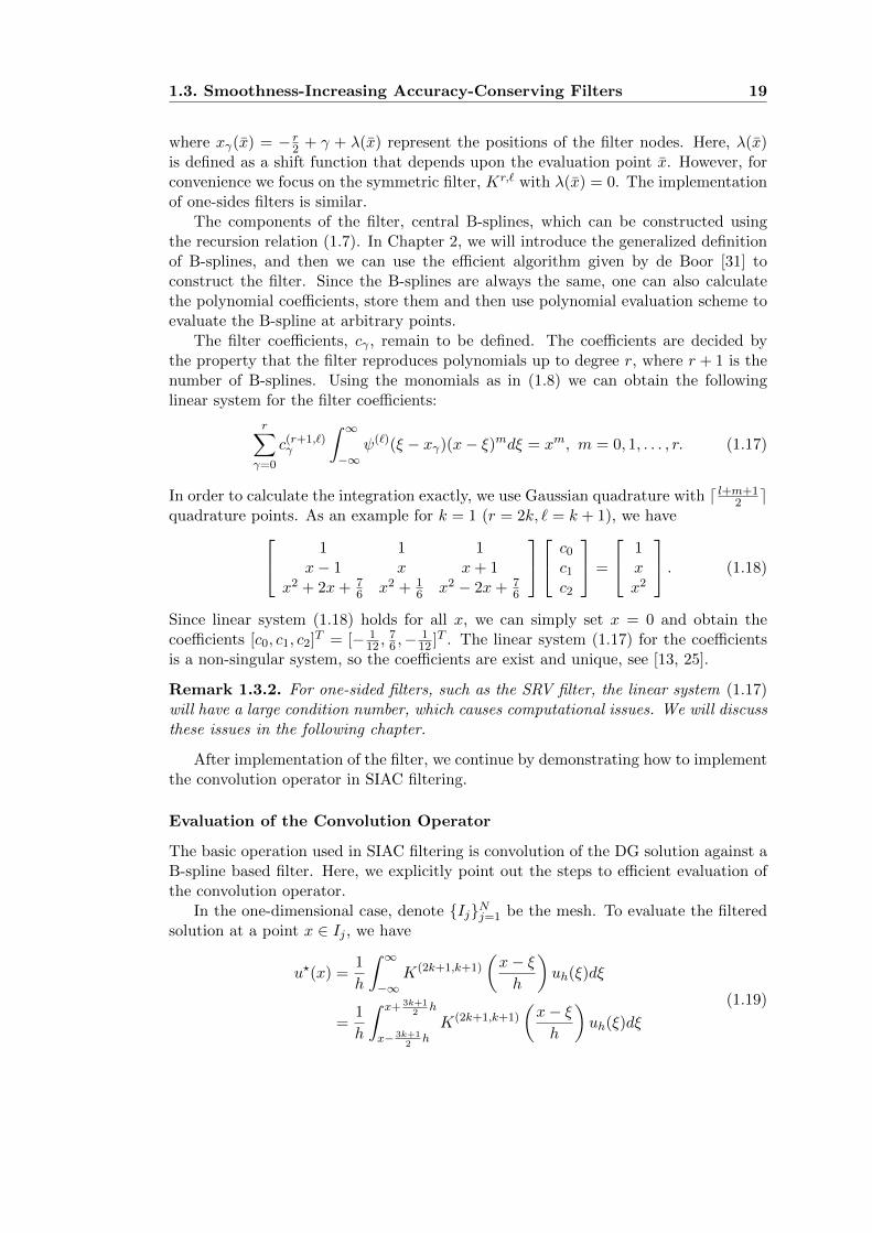
1.3. Smoothness-Increasing Accuracy-Conserving Filters 19
where xγ(x) = − r2 + γ + λ(x) represent the positions of the filter nodes. Here, λ(x)
is defined as a shift function that depends upon the evaluation point x. However, forconvenience we focus on the symmetric filter, Kr,` with λ(x) = 0. The implementationof one-sides filters is similar.
The components of the filter, central B-splines, which can be constructed usingthe recursion relation (1.7). In Chapter 2, we will introduce the generalized definitionof B-splines, and then we can use the efficient algorithm given by de Boor [31] toconstruct the filter. Since the B-splines are always the same, one can also calculatethe polynomial coefficients, store them and then use polynomial evaluation scheme toevaluate the B-spline at arbitrary points.
The filter coefficients, cγ , remain to be defined. The coefficients are decided bythe property that the filter reproduces polynomials up to degree r, where r + 1 is thenumber of B-splines. Using the monomials as in (1.8) we can obtain the followinglinear system for the filter coefficients:
r∑γ=0
c(r+1,`)γ
∫ ∞
−∞ψ(`)(ξ − xγ)(x− ξ)mdξ = xm, m = 0, 1, . . . , r. (1.17)
In order to calculate the integration exactly, we use Gaussian quadrature with d l+m+12 e
quadrature points. As an example for k = 1 (r = 2k, ` = k + 1), we have 1 1 1x− 1 x x+ 1
x2 + 2x+ 76 x2 + 1
6 x2 − 2x+ 76
c0c1c2
=
1xx2
. (1.18)
Since linear system (1.18) holds for all x, we can simply set x = 0 and obtain thecoefficients [c0, c1, c2]
T = [− 112 ,
76 ,−
112 ]
T . The linear system (1.17) for the coefficientsis a non-singular system, so the coefficients are exist and unique, see [13, 25].
Remark 1.3.2. For one-sided filters, such as the SRV filter, the linear system (1.17)will have a large condition number, which causes computational issues. We will discussthese issues in the following chapter.
After implementation of the filter, we continue by demonstrating how to implementthe convolution operator in SIAC filtering.
Evaluation of the Convolution Operator
The basic operation used in SIAC filtering is convolution of the DG solution against aB-spline based filter. Here, we explicitly point out the steps to efficient evaluation ofthe convolution operator.
In the one-dimensional case, denote IjNj=1 be the mesh. To evaluate the filteredsolution at a point x ∈ Ij , we have
u?(x) =1
h
∫ ∞
−∞K(2k+1,k+1)
(x− ξh
)uh(ξ)dξ
=1
h
∫ x+ 3k+12
h
x− 3k+12
hK(2k+1,k+1)
(x− ξh
)uh(ξ)dξ
(1.19)

20 Chapter 1. Background
The integration in (1.19) is calculated by Gauss quadrature with k + 1 quadraturepoints. However, both the DG solution and the filter are piecewise polynomials. There-fore, we have to divide the support, supp(K(x)) =
[x− 3k+1
2 h, x+ 3k+12 h
]into many
subintervals, such that both the DG solution and the filter are polynomials on eachsubinterval. First, consider the discontinuities of the DG solution. We can write (1.19)as
u?(x) =1
h
∑Ii+j∩supp(K(x))6=∅
∫Ii+j
K(2k+1,k+1)
(x− ξh
)uh(ξ)dξ. (1.20)
Then we divide the elements Ii+j into several subintervals that Ii+j =ni+j⋃α=1
Iαi+j ac-
cording to the breaks of the filter such that on each subinterval Iαi+j the filter is apolynomial, ∫
Ii+j
K(2k+1,k+1)
(x− ξh
)uh(ξ)dξ
=
ni+j∑α=1
∫Iαi+j
K(2k+1,k+1)
(x− ξh
)uh(ξ)dξ.
(1.21)
Finally, we can apply the Gauss quadrature to calculate the integration on subintervalsIαi+j . Usually, for uniform meshes we divide each element Ii+j into two subintervals,but for nonuniform meshes the number of subintervals is dependent on the mesh. Tospeed up the filtering process, sometimes it is possible to use inexact integration, see[50]. However, step (1.20) is necessary. The step, which divides the integration regioninto subintervals according to the filter breaks, is also needed for calculating the linearsystem (1.17).
In multi-dimensions, the filter is a tensor product of the one-dimensional filters.The implementation of the multi-dimensional SIAC filter over rectangular meshes isthe same. For triangular meshes, the principles are the same and one can find thedetails in [48].

2Position-Dependent SIAC Filters
2.1 Introduction
When judging the value of numerical methods, the practical usage and computationalconsiderations are always a criteria. As introduced in Chapter 1, due to its symmetricproperty, the symmetric SIAC filter (1.6) can not be applied near domain boundariesor discontinuities of the exact solution, which is impractical in practice. To overcomethis disadvantage, two one-sided filters, the RS filter (1.12) and the SRV filter (1.14),were introduced. However, these still have some deficiencies which are discussed in thefollowing.
2.1.1 The Deficiencies of the RS and SRV Filters
• Theoretical Considerations
As mentioned in Chapter 1, the main difference between the RS filter (1.12) andthe SRV filter (1.14) is the number of B-splines. In order to reduce the errors of the RSfiltered solution, the SRV filter increases the number of B-splines from 2k+1 to 4k+1.The strategy of using 4k + 1 B-splines seems work well as in [65] and Example 1.3.6,however, the actual story is more complicated. One can easily find a counterexamplethat demonstrates using 4k+1 B-splines makes filtered solutions worse than using only2k + 1 B-splines for some examples. A simple one of these is the L2 projection of thewave functions sin(2λπx) over a uniform mesh with N elements. For large λ using theSRV filter leads to a worse result compared to using the RS filter, see Figure 2.1. Thedetails of dealing wave functions are presented in Chapter 6.
To explain this occurrence, one has to check the error estimate of the filteredsolutions. First, we write the generalized formula of SIAC filters as
K(r+1,`)(x) =r∑
γ=0
c(r+1,`)γ ψ(`)(x− xγ(x)), (2.1)
where xγ depends on the location of the evaluation point x. Formula (2.1) can be usedto represent the symmetric filter (1.6), the RS filter (1.12) and the SRV filter (1.14).
21

22 Chapter 2. Position-Dependent SIAC Filters
5 6 7 8 9 10λ
10−2
10−1
100
101
102
103
|erro
r|
P3, N = 40
RS filterSRV filter
Figure 2.1: Comparison of the RS filtered errors (black) and the SRV filtered errors(red) for the L2 projection of sin(2πλx) over a uniform mesh.
Similar to the proof of Theorem 1.3.4, for uniform meshes, we have
‖u− u?h‖0,Ω0 ≤ ‖u−K(r+1,`)h ? u‖0,Ω0 + ‖K
(r+1,`)h ? (u− uh)‖0,Ω0
≤ Θ1 +Θ2,
where
Θ1 = ‖u−K(r+1,`)h ? u‖0,Ω0 ≤
hr+1
(r + 1)!C1|u|r+1, (Equation (1.8))
and
Θ2 = C0
∑|α|≤`
‖DαK(r+1,`)h ? (u− uh)‖−`,Ω1/2
, (Lemma 1.2.2)
≤ C0C1
∑|α|≤`
‖∂αh (u− uh)‖−`,Ω1
≤ C1C2h2k+1, (Theorem 1.2.1)
here Ω0 + supp(K(r+1,`)H ) ⊂ Ω1/2 and Ω1/2 + supp(K
(r+1,`)H ) ⊂ Ω1.
Now, we have
‖u− u?h‖0,Ω0 ≤hr+1
(r + 1)!C1|u|r+1 + C1C2h
2k+1, (2.2)
where C2 is a constant related to the DG approximation and
C1 = supx∈Ω
κ(x), where κ(x) =
r∑γ=0
|c(r+1,k+1)γ | (2.3)

2.1. Introduction 23
is determined by the filter coefficients. In addition, we note that the filter coefficientsare dependent on the location of the evaluation point x.
One can see that increasing the number of B-splines can increase the order of thefirst term in (2.2), but it has no effect on the second term. Another important factoris the constant C1 (or κ), which depends on the filter coefficients. Figure 2.2 showsthe values of κ with respect to the location of the evaluation point.
P3 P4
0 0.2 0.4 0.6 0.8 1.0
x
101
102
103
104
105
106
107
κ(x)
RS FilterSRV Filter
0 0.2 0.4 0.6 0.8 1.0
x
101
102
103
104
105
106
107
κ(x)
RS FilterSRV Filter
Figure 2.2: κ(x) in (2.3) for: the RS filter (1.12) and the SRV filter (1.14) in errorestimate (2.2) with respect the location of the evaluation point. Left: P3 polynomials.Right: P4 polynomials.
The two components of the above error estimate are the error constant and theaccuracy order. Comparing to the RS filter, the SRV filter maintains the same accu-racy order and the error constant is significantly increased, which are the theoreticaldeficiencies of the SRV filter compared to the RS filter. However, if filtering an exactsolution that is sufficiently smooth, using the SRV filter leads to a better accuracythan using the RS filter, see [39].• Computational ConsiderationsIn addition to the theoretical estimates, computational considerations are impor-
tant to consider when applying a technique to real world problems.First, the SRV filter is constructed with 4k + 1 central B-splines, which increased
both the width of the stencil generated and the computational cost (in terms of func-tions evaluations) a disproportionate amount compared to the symmetric filter. Also,when calculating the filter coefficients using the linear system (1.17), one has to useGaussian quadrature with d5k2 + 1e quadrature points.
Second, the SRV filter requires the use of multiple precision (at least quadruple) forP3 and higher degree polynomials to obtain consistent and meaningful results, whichmakes it highly unsuitable for practical CPU-based computations and certainly GPUcomputing. Figure 2.3 shows the significant round-off error near the boundaries whenusing double precision for filtering the L2 projection of a sine function. The round-off
error is due to the huge filter coefficients c(4k+1,k+1)γ , and the enormous condition
number of the linear system (1.17).
24 Chapter 2. Position-Dependent SIAC Filters
Third, the numerical performances of the former filters are not satisfactory fornonlinear equations and nonuniform meshes, see numerical examples in Section 2.4.
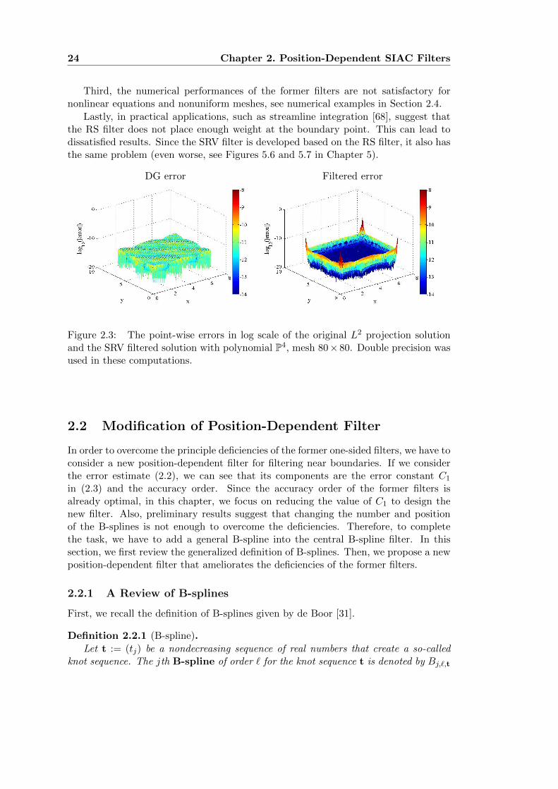
Lastly, in practical applications, such as streamline integration [68], suggest thatthe RS filter does not place enough weight at the boundary point. This can lead todissatisfied results. Since the SRV filter is developed based on the RS filter, it also hasthe same problem (even worse, see Figures 5.6 and 5.7 in Chapter 5).
DG error Filtered error
Figure 2.3: The point-wise errors in log scale of the original L2 projection solutionand the SRV filtered solution with polynomial P4, mesh 80× 80. Double precision wasused in these computations.
2.2 Modification of Position-Dependent Filter
In order to overcome the principle deficiencies of the former one-sided filters, we have toconsider a new position-dependent filter for filtering near boundaries. If we considerthe error estimate (2.2), we can see that its components are the error constant C1
in (2.3) and the accuracy order. Since the accuracy order of the former filters isalready optimal, in this chapter, we focus on reducing the value of C1 to design thenew filter. Also, preliminary results suggest that changing the number and positionof the B-splines is not enough to overcome the deficiencies. Therefore, to completethe task, we have to add a general B-spline into the central B-spline filter. In thissection, we first review the generalized definition of B-splines. Then, we propose a newposition-dependent filter that ameliorates the deficiencies of the former filters.
2.2.1 A Review of B-splines
First, we recall the definition of B-splines given by de Boor [31].
Definition 2.2.1 (B-spline).
Let t := (tj) be a nondecreasing sequence of real numbers that create a so-calledknot sequence. The jth B-spline of order ` for the knot sequence t is denoted by Bj,`,t

2.2. Modification of Position-Dependent Filter 25
and is defined, for ` = 1, by the rule
Bj,1,t(x) =
1, tj ≤ x < tj+1;0, otherwise.
In particular, tj = tj+1 leads to Bj,1,t = 0. For ` > 1,
Bj,`,t(x) = ωj,k,tBj,`−1,t + (1− ωj+1,`,t)Bj+1,`−1,t,
with
ωj,`,t(x) =x− tj
tj+`−1 − tj.
This notation will be used to create a new filter near the boundaries.A central B-spline of order ` has a knot sequence that is uniformly spaced and
symmetrically distributed
t = − `2,−`− 2
2, · · · , `− 2
2,`
2.
For convenience, we denote ψ(`)t (x) to be the 0th B-spline of order ` for the knot
sequence t,
ψ(`)t (x) = B0,`,t(x).
Remark 2.2.1. The knot sequence t also represents the so-called breaks of the B-spline. The B-spline in the region [ti, ti+1), i = 0, . . . , ` − 1 is a polynomial of degree`−1, but in the entire support [t0, t`], the B-spline is a piecewise polynomial. When theknots (tj) are sampled in a symmetric and equidistant fashion, the B-spline is calleda central B-spline. Notice that a central B-spline (1.7) is a subset of this definitionwhere the knots are equally-spaced. This new notation provides more flexibility thanthe previous central B-spline notation.
2.2.2 New Position-Dependent SIAC Filter
We begin by restating the definition of the SIAC filter through the definition of theknots defining the B-splines used in the filter. We recall that the generalized definitionof the filter relied on r + 1 central B-splines of order `. B-splines were then definedautomatically through a knot sequence t := (tj). Before we deduce the new boundaryfilter, we introduce a new definition: knot matrix.
Definition 2.2.2 (Knot matrix).A knot matrix, T, is an n×m matrix such that the γ−th row, T(γ), of the matrix
T is a knot sequence with `+ 1 elements (i.e., m = `+ 1) that are used to create the
B-spline ψ(`)T(γ)(x). The number of rows n is specified based on the number of B-splines
used to construct the filter.
For example, the knot matrix for the symmetric filter (1.6) has components givenby
T (i, j) = − `2+ j + i− r
2, i = 0, . . . , r; and j = 0, . . . , `.

26 Chapter 2. Position-Dependent SIAC Filters
More specifically, consider the filter for DG solutions of degree k = 1. For the sym-metric filter (` = 2 and r = 2), the elements of the knot matrix Tsym are given by
Tsym =
−2 −1 0−1 0 10 1 2
.
For the RS filter (1.12), which uses only 2k+ 1 central B-splines at the left boundary,the knot matrix TRS is given by
TRS =
−4 −3 −2−3 −2 −1−2 −1 0
.
For the SRV filter (1.14), which uses 4k + 1 central B-spline at the left boundary, theknot matrix TSRV is given by
TSRV =
−6 −5 −4−5 −4 −3−4 −3 −2−3 −2 −1−2 −1 0
.
Therefore, we can use Definition 2.2.2 to rewrite the symmetric filter (1.6) in termsof a knot matrix as follows
K(2k+1,k+1)Tsym
(x) =
2k∑γ=0
c(2k+1,k+1)γ ψ
(k+1)Tsym(γ)(x).
Now we can define the new filter by generating a knot matrix.Definition 2.2.2 alone is not enough to create the boundary filter we wish to propose.
We must impose further restrictions on the knot matrix. First, for convenience werequire
T (γ, 0) ≤ T (γ, 1) ≤ · · · ≤ T (γ, `), for γ = 0, . . . , r,
andT (γ + 1, 0) ≤ T (γ, `), for γ = 0, . . . , r − 1.
Second, the knot matrix, T, should satisfy
T (0, 0) ≥ x− xRh
and T (r, `) ≤ x− xLh
,
where h is the element size for a uniform mesh. This requirement is derived from thesupport of the B-spline as well as the support of the filter needing to remain inside
the domain. Recall that the support of the B-spline ψ(`)T(γ) is [T (γ, 0), T (γ, `)], and the
support of the filter is [T (0, 0), T (r, `)]. For any x ∈ [xL, xR], the filtered solution atpoint x can then be written as
u?(x) = K(r+1,`)hT ? uh(x) =
∫ ∞
−∞K
(r+1,`)hT (x− ξ)uh(ξ)dξ
=
∫ x−hT (0,0)
x−hT (r,`)K
(r+1,`)hT (x− ξ)uh(ξ)dξ,

2.2. Modification of Position-Dependent Filter 27
where hT represents the scaled knot matrix. For the boundary regions, we force theinterval [x − hT (r, `), x − hT (0, 0)] to remain inside the domain Ω = [xL, xR]. Thisimplies that
xL ≤ x− hT (r, `), x− hT (0, 0) ≤ xR,
and hence the requirement of T (0, 0) ≥ x−xRh and T (r, `) ≤ x−xL
h . Finally, we requirethat the filter remain as symmetric as possible. This means the knots should be chosenas
Left : T ← T −(T (r, `)− x− xL
h
), for
x− xLh
<3k + 1
2,
Right : T ← T −(T (0, 0)− x− xR
h
), for
xR − xh
<3k + 1
2.
This shifting will increase the error and it is therefore still necessary to increase thenumber of B-splines used in the filter.
Because the symmetric filter yields superconvergence results, we wish to retain theoriginal form of the filter as much as possible. Near the boundary, where the symmetricfilter cannot be applied, we keep the 2k+1 shifted central B-splines and add only onegeneral B-spline. We keep the notation r + 1 = 2k + 1 associated with the number ofcentral B-splines. To avoid increasing the spatial support of the filter, we will choosethe knots of this general B-spline dependent upon the knots of the 2k + 1 centralB-splines in the following way: near the left boundary, we let the first 2k+1 B-splinesbe central B-splines whereas the last B-spline will be a general spline. The elementsof knot matrix are then given by
T (i, j) =
−`− r + j + i+ x−xL
h , 0 ≤ i ≤ 2k, 0 ≤ j ≤ `;x−xL
h − 1, i = 2k + 1, j = 0;x−xL
h , i = 2k + 1, j = 1, . . . , `.
The filter coefficients are decided by the linear system (1.17), which reproducing poly-nomials up to degree r + 1. For the left one-sided filter with scaling h, we have
K(r+1,`)hT (x) =
r+1∑γ=0
c(r+1,`)γ ψ
(`)hT(γ)(x),
where r + 1 = 2k + 1 is the number of central B-splines and T(γ) represents the γ-throw of the knot matrix T. For the central B-splines, γ = 0, . . . , 2k and
ψ(`)hT(γ)(x) =
1
hψ(`)T(γ)
(xh
).
The added B-spline is a monomial defined as
ψ(`)hT(r+1)(x) =
1
hx`−1T(r+1)
(xh
),
where
x`−1T(r+1) =
(x− T (r + 1, 0))`−1 , T (r + 1, 0) ≤ x ≤ T (2k + 1, `);0, otherwise.

28 Chapter 2. Position-Dependent SIAC Filters
Therefore near the left boundary, the filter can be rewritten as
K(r+1,`)hT (x) =
r∑γ=0
c(r+1,`)γ ψ
(`)hT(γ)(x)︸ ︷︷ ︸
r + 1 = 2k + 1 central B-splines
+ c(r+1,`)r+1 ψ
(`)hT(r+1)(x)︸ ︷︷ ︸
General B-spline
. (2.4)
Similarly, we can design the new filter near the right boundary, where the generalB-spline is given by
ψ(`)T(0)(x) = x`−1
T(0) =
(T (0, `)− x)`−1 , T (0, 0) ≤ x ≤ T (r + 1, `);
0, otherwise.
The elements of the knot matrix for the right boundary filter are defined as
T (i, j) =
x−xR
h , i = 0, j = 0, . . . , `− 1;x−xR
h + 1, i = 0, j = `;j + i− 1 + x−xR
h , 1 ≤ i ≤ r + 1, 0 ≤ j ≤ `,
and the form of the filter is then
K(r+1,`)hT (x) = c
(r+1,`)0 ψ
(`)hT(0)(x) +
r+1∑γ=1
c(r+1,`)γ ψ
(`)hT(γ)(x).
We note that this “extra” B-spline is used only when x−xLh < 3k+1
2 or xR−xh < 3k+1
2 ,otherwise the coefficient of the “extra” B-spline becomes zero when solving the linearsystem (1.17), and then the filter becomes the symmetric central B-spline filter.
Example 2.2.1. We present a concrete example for the P1 case with ` = 2. In thiscase, the knot matrices for our newly proposed filter at the left and right boundariesare
TLeft =
−4 −3 −2−3 −2 −1−2 −1 0−1 0 0
, TRight =
0 0 10 1 21 2 32 3 4
.
The following plot illustrates how to use the knot matrix to construct the filter. Theknots and respective B-spline are in same color, the filter is in red.
TLeft =
−4 −3 −2−3 −2 −1−2 −1 0−1 0 0
,
In the left figure, the three equally dis-tributed blue (green, cyan) points repre-sent the central B-spline in color blue(green, cyan), and the three black pointsrepresent the general B-spline (two multi-ple points at 0).
−4 −3 −2 −1 0
−2
−1
0
1
2
3
4
5

2.3. Theoretical Results 29
These new knot matrices are 4× 3 matrices where, in the case of the filter for theleft boundary, the first three rows express the knots of the three central B-splines andthe last row expresses the knots of the general B-spline. For the filter applied to theright boundary, the first row expresses the knots of the general B-spline and the lastthree rows express the knots of the central B-splines.
Comparing the new knot matrix with the one used to obtain the SRV filter, wecan see that they have the same number of columns, which indicates that they use thesame order of B-splines. There are fewer rows in the new matrix (2k + 2) than thenumber of rows from the SRV filter (4k + 1). This indicates that the new filter usesfewer B-splines than the SRV filter.
To compare all existing one-sided filters, we plot these filters used at the left bound-ary for k = 2. Figure 2.4 illustrates that the new position-dependent SIAC filter placesmore weight on the evaluation point than the former filters, and the SRV filter hasa significantly larger magnitude and support which we observed to cause problems,especially for higher-order polynomials (such as P3 or P4). For this example, usingthe filter for quadratic approximations, the scaling of the SRV filter has a range from−150 to 150 versus −5 to 5 for the newly proposed filter.
RS filter SRV filter New filter
−12 −8 −4 0−15−10−5
05
1015
−12 −8 −4 0−150−100−50
050
100150
−12 −8 −4 0−5
0
5
Figure 2.4: (Left) RS filter (1.12), (Center) SRV filter (1.14) and (Right) the newlyproposed filter with k = 2. The filtered point is at boundary x = 0.
2.3 Theoretical Results
The previous section introduced a new filter to reduce the errors of dG approximationswhile attempting to ameliorate the issues concerning the former filters. In this section,we discuss the theoretical results of the newly defined boundary filter.
2.3.1 Local Error Estimate in the Negative Order Norm
First of all, we point out there is a minor flaw in the theoretical foundation of one-sided filters. The error estimate in the negative order norm, given in Theorem 1.2.1,assumes periodic boundary conditions. It follows that the error estimate of the SRVfilter given in [39] is under the same periodic boundary assumption. The periodicboundary assumption is unnatural for one-sided filters since with the periodic bound-ary assumption we can use the symmetric filter directly. To ameliorate this minor

30 Chapter 2. Position-Dependent SIAC Filters
flaw, we present an alternative error estimate of the DG solution in the negative ordernorm.
Lemma 2.3.1. Let u be the exact solution of a linear hyperbolic equation (1.1), andlet uh be the DG approximation. Then the negative order norm estimate of u − uhsatisfies
‖(u− uh)(T )‖−(k+1),Ω ≤ Ch2k+1. (2.5)
Note: comparing to Theorem 1.2.1, the periodic boundary condition was removed.
Proof. First we give a dual problem of equation (1.1) by
ϕt +d∑
i=1
aiϕxi − a0ϕ = 0, ϕ(x, T ) = Φ(x).
The DG approximation satisfies scheme (1.2)
((uh)t, vh)K −d∑
i=1
(aiuh, (vh)xi)K
+d∑
i=1
∫∂K
aiuhvhnids+ (a0uh, vh) = 0,
By applying the dual problem, we obtain
d
dt(u, ϕ)K = −
d∑i=1
∫∂K
aiuϕnids.
and
(u, ϕ)K(T ) = (u, ϕ)K(0)−∫ T
0
(d∑
i=1
∫∂K
aiuϕnids
)dt.
Note: the original proof in [25] assumed periodic boundary conditions. Then the term∫ T
0
(d∑
i=1
∫∂K
aiuϕnids
)dt is counteracted by summing up for all K ∈ Th in [25].
Without assuming the periodic boundary conditions the term remains in the analysis.
Then we have
((u− uh)(T ),Φ)K = (u− uh, ϕ)(T )
=(u− uh, ϕ)K(0)−∫ T
0
(d∑
i=1
∫∂K
aiuϕnids
)dt−
∫ T
0
d
dt(uh, ϕ)Kdt.

2.3. Theoretical Results 31
Considering ddt(uh, ϕ)K in the third term,
d
dt(uh, ϕ)K = ((uh)t, ϕ)K + (uh, ϕt)K ,
= ((uh)t, ϕ− vh)K + ((uh)t, vh)K + (uh, ϕt)K (vh ∈ V kh )
= ((uh)t, ϕ− vh)K + (uh,
d∑i=1
ai(vh)xi)K
−d∑
i=1
∫∂K
aiuhvhnids− (a0uh, vh)K + (uh, ϕt)K
= ((uh)t + a0uh, ϕ− vh)K
−
(uh,
d∑i=1
ai(ϕ− vh)xi
)K
−d∑
i=1
∫∂K
aiuhvhnids,
=
((uh)t +
d∑i=1
ai(uh)xi + a0uh, ϕ− vh
)K
−d∑
i=1
∫∂K
aiuh(ϕ− vh)nids−d∑
i=1
∫∂K
aiuhvhnids,
= −d∑
i=1
∫∂K
aiuh(ϕ− vh)nids−d∑
i=1
∫∂K
aiuhvhnids,
substituting above formula back, we have
((u− uh)(T ),Φ)K
= (u− uh, ϕ)K(0)−∫ T
0
(d∑
i=1
∫∂K
aiuϕnids
)dt
+
∫ T
0
(d∑
i=1
∫∂K
ai (uh(ϕ− vh)ni + uhvhni) ds
)dt
= (u− uh, ϕ)K(0)−∫ T
0
(d∑
i=1
∫∂K
ai(u− uh)ϕnids
)dt
+
∫ T
0
(d∑
i=1
∫∂K
ai(uh − uh)(ϕ− vh)nids
)dt
Since the first and the third term are identical to the proof in [25], we need onlyconsider the second term. According to [4, 15], the DG solution has superconvergenceproperty for its numerical flux
|d∑
i=1
∫∂K
(u− uh)| ≤ Ch2k+1,

32 Chapter 2. Position-Dependent SIAC Filters
which does not rely on the periodic boundary condition. Then, for the second term,we have ∫ T
0
(d∑
i=1
∫∂K
ai(u− uh)ϕnids
)dt ≤
∫ T
0Ch2k+1‖ϕ‖k+1,Ωdt.
Summing up over all K ∈ Th, we obtain (2.5).
Remark 2.3.1. Compared to the original theorem, Lemma 2.3.1 theoretically confirmsthat the periodic boundary conditions are not necessary. It reveals the fact that the filterhas compact support and needs only local information of the DG approximation. Theerror estimates for divided differences of the DG approximation ∂αhuh are similar, andwe will address the details in Chapter 4.
2.3.2 Theoretical Results in the Uniform Case
First, we discuss the theoretical results of the new one-sided filter for uniform meshes.Specifically, for k = 1 it is globally superconvergent of order three. For higher degreepolynomials, it is possible to obtain superconvergence only in the interior of the domain.
Recall that the new scaled filter has the form
K(r+1,`)hT (x) =
r+1∑γ=0
c(r+1,`)γ ψ
(`)hT(γ)(x).
In the interior of the domain the symmetric filter is used. It consists of 2k + 1 centralB-splines,
K(2k+1,`)hT (x) =
2k∑γ=0
c(2k+1,`)γ ψ
(`)hT(γ)(x),
and, near the left boundary the new one-sided filter can be written as
K(2k+1,`)hT (x) =
2k∑γ=0
c(2k+1,`)γ ψ
(`)hT(γ)(x)
+ c(2k+1,`)2k+1 ψ
(`)hT(2k+1)(x),
where 2k+1 central B-splines are used together with one general B-spline. The scaled
filter K(r+1,`)hT has the property that the convolution K
(r+1,`)hT ?uh only uses information
inside the domain Ω.
Theorem 2.3.2. Under the same conditions in Theorem 1.3.4, let u?h(x) = (K(r+1,`)hT ?
uh)(x) be the solution obtained by applying the newly proposed filter which uses r+1 =2k+1 central B-splines of order ` = k+1 and one general B-spline in boundary regions.Then the filtered solution has the following properties:
(i) ‖(u − u?h)(x)‖0,Ω ≤ Ch3 for k = 1. That is, u?h(x) is globally superconvergent oforder three for linear approximations.
(ii) ‖(u − u?h)(x)‖0,Ω\suppKs ≤ Chr+1 when r + 1 ≤ 2k + 1 central B-splines areused in the filter. Here suppKs represents the support of the symmetric filter.Thus, u?h(x) is superconvergent in the interior of the domain.
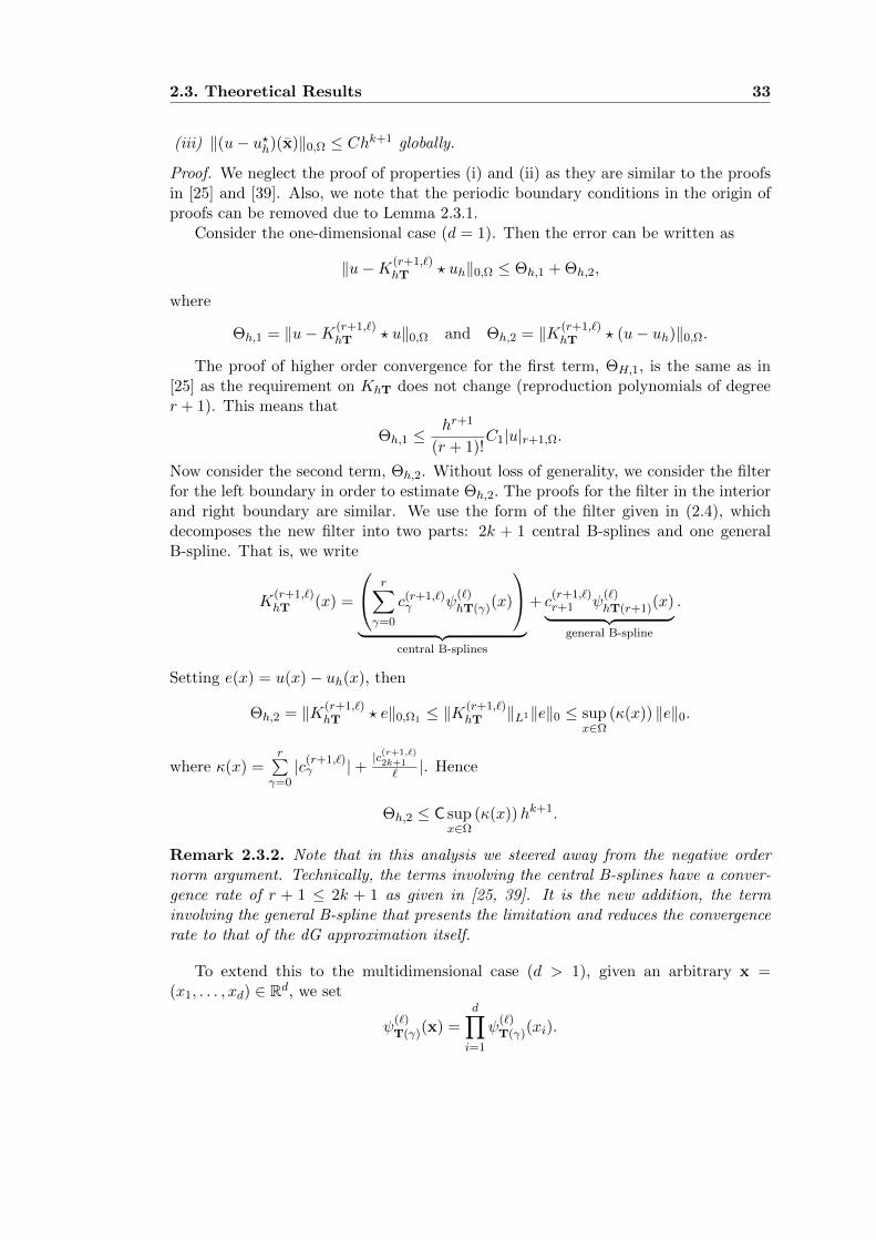
2.3. Theoretical Results 33
(iii) ‖(u− u?h)(x)‖0,Ω ≤ Chk+1 globally.
Proof. We neglect the proof of properties (i) and (ii) as they are similar to the proofsin [25] and [39]. Also, we note that the periodic boundary conditions in the origin ofproofs can be removed due to Lemma 2.3.1.
Consider the one-dimensional case (d = 1). Then the error can be written as
‖u−K(r+1,`)hT ? uh‖0,Ω ≤ Θh,1 +Θh,2,
where
Θh,1 = ‖u−K(r+1,`)hT ? u‖0,Ω and Θh,2 = ‖K
(r+1,`)hT ? (u− uh)‖0,Ω.
The proof of higher order convergence for the first term, ΘH,1, is the same as in[25] as the requirement on KhT does not change (reproduction polynomials of degreer + 1). This means that
Θh,1 ≤hr+1
(r + 1)!C1|u|r+1,Ω.
Now consider the second term, Θh,2. Without loss of generality, we consider the filterfor the left boundary in order to estimate Θh,2. The proofs for the filter in the interiorand right boundary are similar. We use the form of the filter given in (2.4), whichdecomposes the new filter into two parts: 2k + 1 central B-splines and one generalB-spline. That is, we write
K(r+1,`)hT (x) =
r∑γ=0
c(r+1,`)γ ψ
(`)hT(γ)(x)
︸ ︷︷ ︸
central B-splines
+ c(r+1,`)r+1 ψ
(`)hT(r+1)(x)︸ ︷︷ ︸
general B-spline
.
Setting e(x) = u(x)− uh(x), then
Θh,2 = ‖K(r+1,`)hT ? e‖0,Ω1 ≤ ‖K
(r+1,`)hT ‖L1‖e‖0 ≤ sup
x∈Ω(κ(x)) ‖e‖0.
where κ(x) =r∑
γ=0|c(r+1,`)γ |+ |c(r+1,`)
2k+1
` |. Hence
Θh,2 ≤ C supx∈Ω
(κ(x))hk+1.
Remark 2.3.2. Note that in this analysis we steered away from the negative ordernorm argument. Technically, the terms involving the central B-splines have a conver-gence rate of r + 1 ≤ 2k + 1 as given in [25, 39]. It is the new addition, the terminvolving the general B-spline that presents the limitation and reduces the convergencerate to that of the dG approximation itself.
To extend this to the multidimensional case (d > 1), given an arbitrary x =(x1, . . . , xd) ∈ Rd, we set
ψ(`)T(γ)(x) =
d∏i=1
ψ(`)T(γ)(xi).
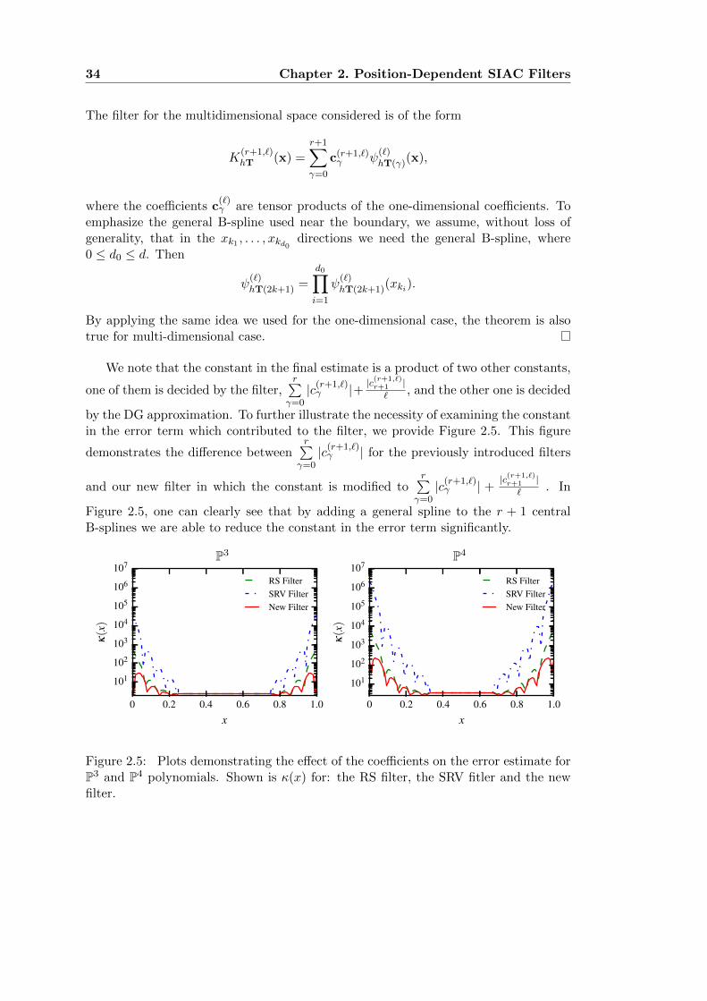
34 Chapter 2. Position-Dependent SIAC Filters
The filter for the multidimensional space considered is of the form
K(r+1,`)hT (x) =
r+1∑γ=0
c(r+1,`)γ ψ
(`)hT(γ)(x),
where the coefficients c(`)γ are tensor products of the one-dimensional coefficients. To
emphasize the general B-spline used near the boundary, we assume, without loss ofgenerality, that in the xk1 , . . . , xkd0 directions we need the general B-spline, where0 ≤ d0 ≤ d. Then
ψ(`)hT(2k+1) =
d0∏i=1
ψ(`)hT(2k+1)(xki).
By applying the same idea we used for the one-dimensional case, the theorem is alsotrue for multi-dimensional case.
We note that the constant in the final estimate is a product of two other constants,
one of them is decided by the filter,r∑
γ=0|c(r+1,`)γ |+ |c(r+1,`)
r+1 |` , and the other one is decided
by the DG approximation. To further illustrate the necessity of examining the constantin the error term which contributed to the filter, we provide Figure 2.5. This figure
demonstrates the difference betweenr∑
γ=0|c(r+1,`)γ | for the previously introduced filters
and our new filter in which the constant is modified tor∑
γ=0|c(r+1,`)γ | + |c(r+1,`)
r+1 |` . In
Figure 2.5, one can clearly see that by adding a general spline to the r + 1 centralB-splines we are able to reduce the constant in the error term significantly.
P3 P4
0 0.2 0.4 0.6 0.8 1.0
x
101
102
103
104
105
106
107
κ(x)
RS FilterSRV FilterNew Filter
0 0.2 0.4 0.6 0.8 1.0
x
101
102
103
104
105
106
107
κ(x)
RS FilterSRV FilterNew Filter
Figure 2.5: Plots demonstrating the effect of the coefficients on the error estimate forP3 and P4 polynomials. Shown is κ(x) for: the RS filter, the SRV fitler and the newfilter.
2.3. Theoretical Results 35
2.3.3 Theoretical Results in the Nonuniform Case
In this section, we give a theoretical interpretation to the computational results pre-sented in [30]. This is done by using the newly proposed filter for nonuniform meshesand showing that the new position-dependent filter maintains the superconvergenceproperty in the interior of the domain for smoothly-varying meshes and is accuracyorder conserving near the boundaries for nonuniform meshes. We begin by definingwhat we mean by a smoothly-varying mesh.
Definition 2.3.1 (Smoothly-Varying Mesh).
Let ξ be a function defined over a uniform mesh on domain Ω ⊂ R, then a smoothly-varying mesh defined over Ω is a nonuniform mesh whose variable x satisfies
x = ξ + f(ξ), (2.6)
where f is a sufficiently smooth function and satisfies
f ′(ξ) > −1, ξ ∈ ∂Ω⇐⇒ ξ + f(ξ) ∈ ∂Ω.
For example, we can choose f(ξ) = 0.5 sin(ξ) over [0, 2π]. The multi-dimensionaldefinition can be defined in the same way.
Lemma 2.3.3. Under the same conditions in Theorem 1.2.1, denote ξ to be the vari-able for the uniform mesh defined on Ω with size h, and x be the variable of a smoothly-varying mesh defined in (2.6). Let uh(ξ) be the numerical solution to linear hyperbolicequation (1.1) over uniform mesh ξ, and uh(x) be the approximation over smoothly-varying mesh x, both of them obtained by using the discontinuous Galerkin scheme(1.2). Then the filtered solution obtained by applying SIAC filter Kh(ξ) for uh(ξ) andKH(x) for uh(x) with a proper scaling H, are related by
‖u(x)−KH ? uh(x)‖0,Ω ≤ C‖u(ξ)−Kh ? uh(ξ)‖0,Ω.
Here, the filter K can be any filter we mentioned in the previous section (symmetricfilter, RS filter, SRV filter, and newly proposed position-dependent filter).
This lemma will be important for demonstrating superconvergence for smoothly-varying meshes.
Proof. The proof is straightforward. If the scaling H is properly chosen, a simple map-ping can be done from the smoothly-varying mesh to the corresponding uniform mesh.The result holds if the Jacobian is bounded (from the definition of smoothly-varyingmesh).
‖u(x)−KH ? uh(x)‖20,Ω =
∫Ω(u(x)−KH ? uh(x))
2 dx
x→ξ=
∫Ω(u(ξ)− u?h(ξ))
2 (1 + f ′(ξ))dξ
≤ ‖u(ξ)−Kh ? uh(ξ)‖20,Ω ·max |1 + f ′(ξ)|.
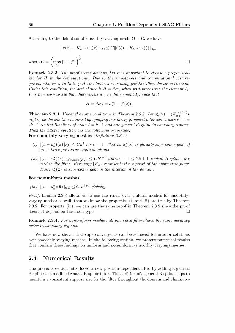
36 Chapter 2. Position-Dependent SIAC Filters
According to the definition of smoothly-varying mesh, Ω = Ω, we have
‖u(x)−KH ? uh(x)‖0,Ω ≤ C‖u(ξ)−Kh ? uh(ξ)‖0,Ω,
where C =
(maxΩ|1 + f ′|
) 12
.
Remark 2.3.3. The proof seems obvious, but it is important to choose a proper scal-ing for H in the computations. Due to the smoothness and computational cost re-quirements, we need to keep H constant when treating points within the same element.Under this condition, the best choice is H = ∆xj when post-processing the element Ij.It is now easy to see that there exists a c in the element Ij, such that
H = ∆xj = h(1 + f ′(c)).
Theorem 2.3.4. Under the same conditions in Theorem 2.3.2. Let u?h(x) = (K(r+1,`)hT ?
uh)(x) be the solution obtained by applying our newly proposed filter which uses r+1 =2k+1 central B-splines of order ` = k+1 and one general B-spline in boundary regions.Then the filtered solution has the following properties:For smoothly-varying meshes (Definition 2.3.1),
(i) ‖(u − u?h)(x)‖0,Ω ≤ Ch3 for k = 1. That is, u?h(x) is globally superconvergent oforder three for linear approximations.
(ii) ‖(u − u?h)(x)‖0,Ω\suppKs ≤ Chr+1 when r + 1 ≤ 2k + 1 central B-splines areused in the filter. Here suppKs represents the support of the symmetric filter.Thus, u?h(x) is superconvergent in the interior of the domain.
For nonuniform meshes,
(iii) ‖(u− u?h)(x)‖0,Ω ≤ C hk+1 globally.
Proof. Lemma 2.3.3 allows us to use the result over uniform meshes for smoothly-varying meshes as well, then we know the properties (i) and (ii) are true by Theorem2.3.2. For property (iii), we can use the same proof in Theorem 2.3.2 since the proofdoes not depend on the mesh type.
Remark 2.3.4. For nonuniform meshes, all one-sided filters have the same accuracyorder in boundary regions.
We have now shown that superconvergence can be achieved for interior solutionsover smoothly-varying meshes. In the following section, we present numerical resultsthat confirm these findings on uniform and nonuniform (smoothly-varying) meshes.
2.4 Numerical Results
The previous section introduced a new position-dependent filter by adding a generalB-spline to a modified central B-spline filter. The addition of a general B-spline helps tomaintain a consistent support size for the filter throughout the domain and eliminates

2.4. Numerical Results 37
the need for a multi-precision package. Also, due to Property 1.3.2 of the symmetricfilter, we know that when the evaluation point moves gradually from the boundaryto the interior region, the new one-sided filter smoothly transforms to the symmetricfilter. This section illustrates the performance of the new position-dependent SIACfilter on uniform and nonuniform (smoothly-varying and random) meshes.
We compare the results to the SRV filter [65]. In order to provide a fair comparisonbetween the SRV and new filters, we mainly show the results using quadruple precisionfor mostly one-dimensional cases. We also provide one result using double precision toshow that quadruple precision is necessary(unnecessary) to use the SRV(new) filter.Furthermore, in order to reduce the computational cost of the filter that uses 4k + 1central B-splines, we neglect to implement the convex combination described in (1.16).This convex combination is not necessary for the new filter, and it has no effect on theaccuracy.
Remark 2.4.1. The SRV filter requires using quadruple precision in the computa-tions to eliminate round-off error, which is more computationally expensive than usingdouble precision. The new filter only requires double precision. In order to give afair comparison between the SRV filter and the new filter, for the one-dimensionalexamples we have used quadruple precision to maintain a consistent computationalenvironment. However, for the two-dimensional examples we have used double preci-sion since quadruple precision is too expensive (approximately ten times slower) formulti-dimensions.
2.4.1 Uniform Meshes
Linear hyperbolic equation
The first example we consider is a linear hyperbolic equation,
ut + ux = 0, (x, t) ∈ [0, 1]× (0, T ]
u(x, 0) = sin(2πx), x ∈ [0, 1].(2.7)
with T = 1 over uniform meshes. The exact solution is a translation of the sinefunction, u(x, t) = sin(2π(x− t)).
The DG solution error and the position-dependent SIAC filtered (SRV and newfilter) error are shown in Table 2.1 for both quadruple precision and double precision.Using quadruple precision, both filters reduce the errors in filtered solution, althoughthe new filter has only a minor reduction in the quality of the error. However, us-ing double precision only the new filter can maintain this error reduction for P3 andP4polynomials. We note that we concentrate on the results for P3 and P4 polynomialsas there is no noticeable difference between double and quadruple precision for P1 andP2 polynomials in the one-dimension.
The point-wise error plots are given in Figures 2.6. When using quadruple precision,the SRV filter can reduce the error of the DG solution better than the new filterfor sufficiently fine meshes. However, it uses 2k − 1 more B-splines than the newlygenerated filter. This difference is noticeable when using double precision, which isalmost ten times faster than using quadruple precision for P3 and P4. For such examples

38 Chapter 2. Position-Dependent SIAC Filters
the new filter performs better both computationally and numerically (in terms oferror). Table 2.1 shows that the former filter can only reduce the error for fine mesheswhen using P4 piecewise polynomials. The new filter performs as good as when usingquadruple precision and reduces the error magnitude at a reduced computational cost.
Additionally, we point out that the accuracy of the SRV filter depends on (1) havinghigher regularity of C4k+1, (2) a well-resolved DG solution, and (3) a wide enoughsupport (at least 5k+1 elements). The same phenomenon will also be observed in thefollowing tests such as for a nonlinear equation. For the new filter, the support sizeremains the same throughout the domain – 3k + 1 elements – and a higher degree ofregularity is not necessary.
Note: In the following examples, all one-dimensional examples are using quadrupleprecision due to the SRV filter, and all two-dimensional examples are using doubleprecision due to the computational cost.
DG SRV Filter New filter
Quadruple precision:
Double precision:
Figure 2.6: Comparison of the point-wise errors of the DG solution, the SRV filter andthe new filter for linear hyperbolic equation (2.7) over uniform meshes with polynomialsP4.
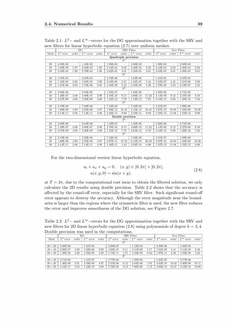
2.4. Numerical Results 39
Table 2.1: L2− and L∞−errors for the DG approximation together with the SRV andnew filters for linear hyperbolic equation (2.7) over uniform meshes.
DG SRV Filter New FilterMesh L2 error order L∞ error order L2 error order L∞ error order L2 error order L∞ error order
Quadruple precisionP1
20 4.02E-03 – 1.45E-02 – 1.98E-03 – 2.80E-03 – 1.98E-03 – 2.80E-03 –40 1.02E-03 1.97 3.82E-03 1.92 2.44E-04 3.02 3.46E-04 3.02 2.44E-04 3.02 3.46E-04 3.0280 2.58E-04 1.99 9.79E-04 1.96 3.02E-05 3.01 4.28E-05 3.01 3.03E-05 3.01 4.28E-05 3.01
P2
20 1.07E-04 – 3.67E-04 – 3.73E-06 – 5.82E-06 – 1.21E-05 – 8.27E-05 –40 1.34E-05 3.00 4.62E-05 2.99 9.42E-08 5.31 1.34E-07 5.44 5.52E-07 4.45 5.31E-06 3.9680 1.67E-06 3.00 5.78E-06 3.00 2.48E-09 5.24 3.52E-09 5.26 4.79E-08 3.53 6.19E-07 3.10
P3
20 2.06E-06 – 6.04E-06 – 1.53E-07 – 1.02E-06 – 2.30E-06 – 8.71E-06 –40 1.29E-07 4.00 3.80E-07 3.99 2.70E-10 9.15 4.00E-10 11.32 4.14E-09 9.12 2.27E-08 8.5880 8.07E-09 4.00 2.38E-08 4.00 1.22E-12 7.79 1.73E-12 7.85 8.18E-12 8.98 1.20E-10 7.56
P4
20 3.19E-08 – 7.02E-08 – 7.53E-03 – 7.33E-02 – 5.31E-07 – 1.99E-06 –40 1.00E-09 4.99 2.25E-09 4.97 1.99E-12 31.82 3.12E-12 34.45 2.97E-10 10.80 1.58E-09 10.3080 3.14E-11 5.00 7.14E-11 4.98 2.23E-15 9.80 3.19E-15 9.93 1.37E-13 11.08 1.55E-12 9.99
Double precisionP3
20 2.06E-06 – 6.04E-06 – 1.53E-07 – 1.02E-06 – 2.30E-06 – 8.71E-06 –40 1.29E-07 4.00 3.80E-07 3.99 2.70E-10 9.15 4.00E-10 11.32 4.14E-09 9.12 2.27E-08 8.5880 8.07E-09 4.00 2.38E-08 4.00 1.25E-12 7.75 3.85E-12 6.70 8.18E-12 8.98 1.20E-10 7.56
P4
20 3.19E-08 – 7.02E-08 – 7.53E-03 – 7.33E-02 – 5.31E-07 – 1.99E-06 –40 1.00E-09 4.99 2.25E-09 4.97 3.97E-11 27.50 6.14E-10 26.83 2.97E-10 10.80 1.58E-09 10.3080 3.14E-11 5.00 7.14E-11 4.98 1.48E-11 1.42 3.28E-10 0.90 1.37E-13 11.08 1.55E-12 9.99
For the two-dimensional version linear hyperbolic equation,
ut + ux + uy = 0, (x, y) ∈ [0, 2π]× [0, 2π],
u(x, y, 0) = sin(x+ y),(2.8)
at T = 2π, due to the computational cost issue to obtain the filtered solution, we onlycalculate the 2D results using double precision. Table 2.2 shows that the accuracy isaffected by the round-off error, especially for the SRV filter. Such significant round-offerror appears to destroy the accuracy. Although the error magnitude near the bound-aries is larger than the regions where the symmetric filter is used, the new filter reducesthe error and improves smoothness of the DG solution, see Figure 2.7.
Table 2.2: L2− and L∞−errors for the DG approximation together with the SRV andnew filters for 2D linear hyperbolic equation (2.8) using polynomials of degree k = 3, 4.Double precision was used in the computations.
DG SRV Filter New FilterMesh L2 error order L∞ error order L2 error order L∞ error order L2 error order L∞ error order
P3
20× 20 3.30E-06 – 1.21E-05 – 2.60E-07 – 1.12E-04 – 2.39E-06 – 1.80E-05 –40× 40 2.06E-07 4.00 7.60E-06 3.99 4.69E-10 9.11 3.11E-09 5.17 7.01E-09 8.41 5.11E-08 8.4680× 80 1.29E-08 4.00 4.76E-08 4.00 1.74E-11 4.75 5.50E-09 -0.82 7.97E-11 6.46 1.02E-09 5.65
P4
20× 20 4.71E-08 – 1.41E-07 – 2.77E-08 – 1.35E-06 – 5.25E-07 – 3.77E-06 –40× 40 1.46E-09 5.01 4.50E-09 4.97 2.55E-08 0.12 2.84E-06 -1.07 3.83E-10 10.42 3.40E-09 10.1180× 80 4.44E-11 5.04 1.43E-10 4.98 2.73E-08 -0.10 7.86E-06 -1.47 3.00E-13 10.31 3.12E-12 10.09
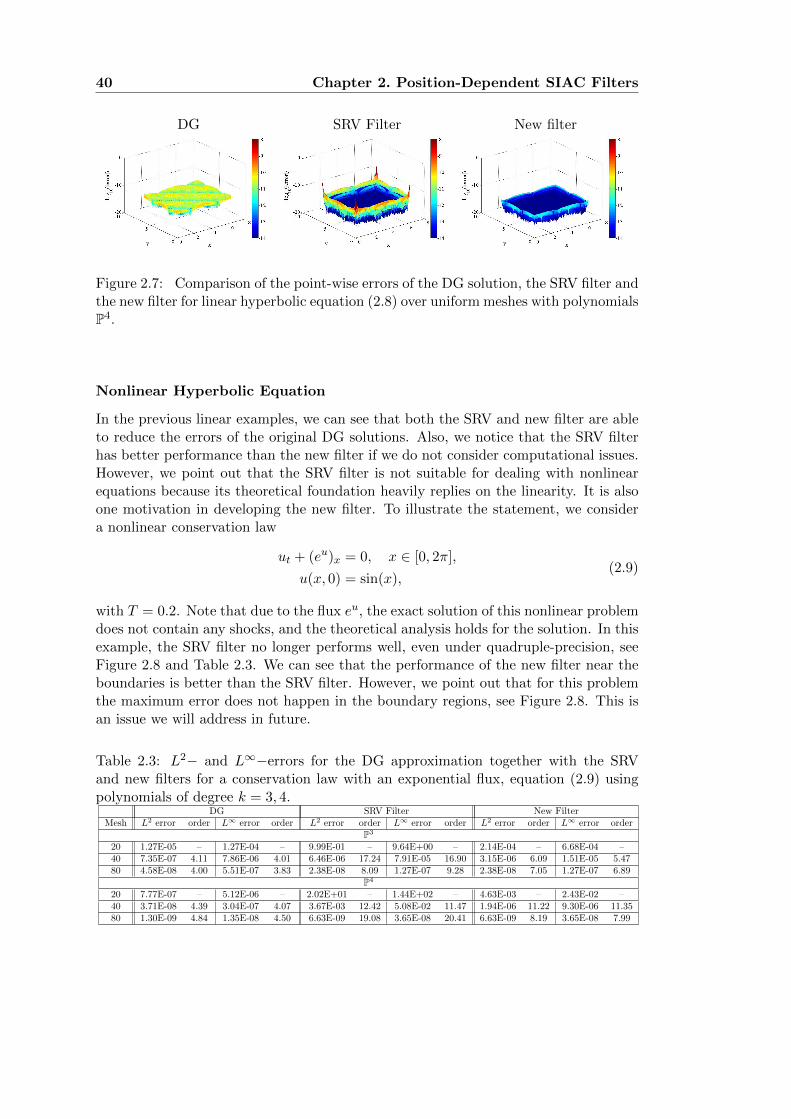
40 Chapter 2. Position-Dependent SIAC Filters
DG SRV Filter New filter
Figure 2.7: Comparison of the point-wise errors of the DG solution, the SRV filter andthe new filter for linear hyperbolic equation (2.8) over uniform meshes with polynomialsP4.
Nonlinear Hyperbolic Equation
In the previous linear examples, we can see that both the SRV and new filter are ableto reduce the errors of the original DG solutions. Also, we notice that the SRV filterhas better performance than the new filter if we do not consider computational issues.However, we point out that the SRV filter is not suitable for dealing with nonlinearequations because its theoretical foundation heavily replies on the linearity. It is alsoone motivation in developing the new filter. To illustrate the statement, we considera nonlinear conservation law
ut + (eu)x = 0, x ∈ [0, 2π],
u(x, 0) = sin(x),(2.9)
with T = 0.2. Note that due to the flux eu, the exact solution of this nonlinear problemdoes not contain any shocks, and the theoretical analysis holds for the solution. In thisexample, the SRV filter no longer performs well, even under quadruple-precision, seeFigure 2.8 and Table 2.3. We can see that the performance of the new filter near theboundaries is better than the SRV filter. However, we point out that for this problemthe maximum error does not happen in the boundary regions, see Figure 2.8. This isan issue we will address in future.
Table 2.3: L2− and L∞−errors for the DG approximation together with the SRVand new filters for a conservation law with an exponential flux, equation (2.9) usingpolynomials of degree k = 3, 4.
DG SRV Filter New FilterMesh L2 error order L∞ error order L2 error order L∞ error order L2 error order L∞ error order
P3
20 1.27E-05 – 1.27E-04 – 9.99E-01 – 9.64E+00 – 2.14E-04 – 6.68E-04 –40 7.35E-07 4.11 7.86E-06 4.01 6.46E-06 17.24 7.91E-05 16.90 3.15E-06 6.09 1.51E-05 5.4780 4.58E-08 4.00 5.51E-07 3.83 2.38E-08 8.09 1.27E-07 9.28 2.38E-08 7.05 1.27E-07 6.89
P4
20 7.77E-07 – 5.12E-06 – 2.02E+01 – 1.44E+02 – 4.63E-03 – 2.43E-02 –40 3.71E-08 4.39 3.04E-07 4.07 3.67E-03 12.42 5.08E-02 11.47 1.94E-06 11.22 9.30E-06 11.3580 1.30E-09 4.84 1.35E-08 4.50 6.63E-09 19.08 3.65E-08 20.41 6.63E-09 8.19 3.65E-08 7.99

2.4. Numerical Results 41
DG SRV Filter New filter
Figure 2.8: Comparison of the point-wise errors of the DG solution, the SRV filterand the new filter for a conservation law with an exponential flux over uniform mesheswith polynomials P4.
SIAC Filtering for Shocks
Although the theorem for the SIAC filter has been established for smooth solutions,it is interesting to investigate the application of SIAC filter to solutions which containshocks. To demonstrate the possibilites of the filtered results for such problems, wepresent the following three examples: First, a discontinuous coefficient equation; sec-ond, a one-dimensional Burgers equation after the shock has developed; and lastly, thedouble Mach reflection problem of the two-dimensional Euler equations.• Variable coefficient equation with stationary shocksIn this example, we consider a variable coefficient equation,
ut + (au)x = f, (x, t) ∈ [0, 1]× (0, T ] (2.10)
with T = 2π. Here, to create discontinuities we consider a discontinuous variablecoefficient
a(x) :=
12 , x ∈ [−1
2 ,12 ],
1, otherwise,
and f(x, t) = 0. The following initial condition was also chosen:
u(x, 0) :=
−2 cos(4πx), x ∈ [−1
2 ,12 ],
cos(2πx), otherwise,
with T = 1. The exact solution is given by
u(x, t) :=
−2 cos(4π(x− 1
2 t)), x ∈ [−12 ,
12 ],
cos(2π(x− t)), otherwise,
which has two stationary shocks.To use the SIAC filter, we have to consider both the discontinuities and the bound-
aries. Similar to the boundary problem, the one-sided filters can also be applied nearthe discontinuities using the same implementation strategy as used near a boundary.

42 Chapter 2. Position-Dependent SIAC Filters
Therefore, we divide the domain into three parts [−1,−12 ], [−
12 ,
12 ] and [12 , 1], then
apply the filter. If the support of the filter is larger than the distance between twoboundaries/discontinuities, we need to change the filter scaling, H, as in [65]. Suchreduction of scaling can have negative consequences on the final results as noted in[43]. Since the two stationary shocks are located at the element interfaces of the DGsolution, the DG solution maintains to keep its k + 1 accuracy order and the errorsare in Table 2.4. Figure 2.9 shows the point-wise error plots. Note that the results arenot as good as in the previous tests due the support size of the filters (even the newfilter) is still quite large for those three subintervals. However, after refining the meshthe accuracy does improve. This is similar to the observations in [43]. Comparing theresults between the SRV and new filter, the new filter has a better performance whenthe distance between two boundaries/discontinuities is small.
DG SRV Filter New filter
Figure 2.9: Comparison of the point-wise errors of the DG solution, the SRV filterand the new filter for discontinuous coefficient equation (2.10) over uniform mesheswith polynomials P4.
Table 2.4: L2− and L∞−errors for the DG approximation together with the SRV andnew filters for the discontinuous coefficient equation (2.10) using polynomials of degreek = 3, 4.
DG SRV Filter New FilterMesh L2 error order L∞ error order L2 error order L∞ error order L2 error order L∞ error order
P3
20 7.39E-04 – 3.12E-03 – 1.97E-01 – 7.75E-01 – 7.34E-02 – 2.70E-01 –40 4.66E-05 3.99 1.92E-04 4.02 1.95E-03 6.66 1.59E-02 5.61 6.50E-04 6.82 3.47E-03 6.2880 2.92E-06 4.00 1.24E-05 3.95 5.09E-05 5.26 7.21E-04 4.46 6.44E-07 9.98 5.95E-06 9.19
P4
20 4.59E-05 – 1.44E-04 – 3.18E+00 – 1.39E+01 – 3.74E-02 – 1.35E-01 –40 1.45E-06 4.99 4.66E-06 4.95 5.83E-03 9.09 2.46E-02 9.14 6.16E-04 5.92 3.26E-03 5.3880 4.54E-08 5.00 1.45E-07 5.01 1.70E-04 5.10 2.11E-03 3.54 9.35E-08 12.69 6.89E-07 12.21
Since the previous examples have already demonstrated superiority of the newfilter, we use only the new filter for the following shock problems.
• 1D Burgers equation with a shock

2.4. Numerical Results 43
In this example, we consider the Burgers equation
ut + uux = 0, (x, t) ∈ [0, 2π]× (0, T ),
u(x, 0) = sin(x),(2.11)
with T = 1. Note that the solution contains a shock at x = π. We have implementedthe symmetric filter in smooth regions and the boundary filter in the elements next tothe boundaries and shocks. No filter is implemented in the element that contains theshock. The results for the point-wise errors are presented in Figure 2.10.
DG After filtering
Figure 2.10: Comparison of the point-wise errors in log scale of the DG solutions andthe filtered solutions (with the new filter) for Burgers equation (2.11), with approxi-mation polynomial is P2.
• Mach reflection problem of the 2D Euler equationsIn this example we apply the new filter to the two dimensional Euler equations for
the double Mach reflection problem. We use the multiwavelet troubled cell indicator ofVuik [66] and plot the results for a zoomed in region of the solution in Figure 2.11. Notethat from the results given for previous examples we expect that the difference whenwe examine the two solutions will be small. However, we do observe some reducedoscillations with the filtered solution.
2.4.2 Smoothly-Varying and Nonuniform Meshes
We emphasize that this is the first time that the position-dependent filters have beentested on nonuniform meshes. Due to Theorem 2.3.4, we using the SRV and new filterwith scaling of H = ∆xj .
Remark 2.4.2. According to [30] we also tested scalings of H = max∆xj, but thescaling H = ∆xj provides better accuracy in boundary regions. Since the motivationof this chapter is to focus on boundaries, we only present results with scaling H =∆xj. However, we point out that the errors produced using a scaling of H = max∆xjare quite similar and often produce smoother errors in the interior of the domain forsmoothly-varying meshes.
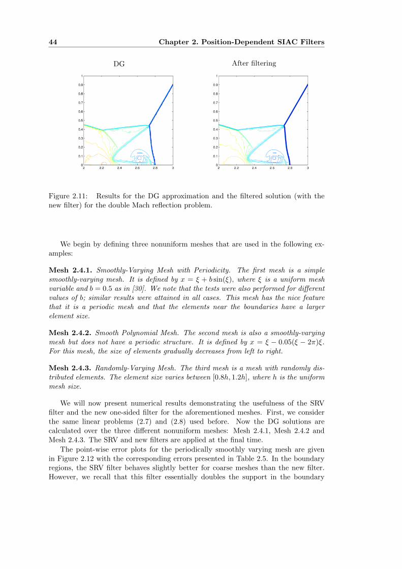
44 Chapter 2. Position-Dependent SIAC Filters
DG After filtering
Figure 2.11: Results for the DG approximation and the filtered solution (with thenew filter) for the double Mach reflection problem.
We begin by defining three nonuniform meshes that are used in the following ex-amples:
Mesh 2.4.1. Smoothly-Varying Mesh with Periodicity. The first mesh is a simplesmoothly-varying mesh. It is defined by x = ξ + b sin(ξ), where ξ is a uniform meshvariable and b = 0.5 as in [30]. We note that the tests were also performed for differentvalues of b; similar results were attained in all cases. This mesh has the nice featurethat it is a periodic mesh and that the elements near the boundaries have a largerelement size.
Mesh 2.4.2. Smooth Polynomial Mesh. The second mesh is also a smoothly-varyingmesh but does not have a periodic structure. It is defined by x = ξ − 0.05(ξ − 2π)ξ.For this mesh, the size of elements gradually decreases from left to right.
Mesh 2.4.3. Randomly-Varying Mesh. The third mesh is a mesh with randomly dis-tributed elements. The element size varies between [0.8h, 1.2h], where h is the uniformmesh size.
We will now present numerical results demonstrating the usefulness of the SRVfilter and the new one-sided filter for the aforementioned meshes. First, we considerthe same linear problems (2.7) and (2.8) used before. Now the DG solutions arecalculated over the three different nonuniform meshes: Mesh 2.4.1, Mesh 2.4.2 andMesh 2.4.3. The SRV and new filters are applied at the final time.
The point-wise error plots for the periodically smoothly varying mesh are givenin Figure 2.12 with the corresponding errors presented in Table 2.5. In the boundaryregions, the SRV filter behaves slightly better for coarse meshes than the new filter.However, we recall that this filter essentially doubles the support in the boundary

2.4. Numerical Results 45
DG SRV Filter New filter
Figure 2.12: Comparison of the point-wise errors of the DG solution, the SRV filterand the new filter for linear hyperbolic equations (1D and 2D) over Mesh 2.4.1 withpolynomials P4. The 2D mesh has 80× 80 elements.
regions. Additionally, we see that the new filter has a higher convergence rate thank + 1 which is better than the theoretically predicted convergence rate.
For the smooth polynomial mesh, Mesh 2.4.2 (without a periodic property), theresults of using the scaling of H = ∆xj are presented in Figure 2.13 and Table 2.5.Unlike the previous example, without the periodic property, the SRV filter leads tosignificantly worse performance. The SRV filter no longer enhances the accuracy orderand has larger errors near the boundaries. On the other hand, the new filter stillimproves accuracy when the mesh is sufficiently refined (N = 40). Numerically thenew filter obtains higher accuracy order than k+ 1. For higher order polynomials, P3
and P4, we see that it achieves accuracy order of 2k + 1, but this is not theoreticallyguaranteed.
Lastly, the filters were applied to DG solutions over a randomly distributed mesh,Mesh 2.4.3. For this randomly-varying mesh, the new filter again reduces the errorsexcept for a very coarse mesh, see Table 2.5. The accuracy order is decreasing com-pared to smoothly-varying mesh examples, but it is still higher than k + 1. Unlikesmoothly-varying meshes, there are more oscillations in the errors if we compare Fig-ure 2.14 with Figure 2.12. However, the oscillations are still reduced compared tothe DG solutions. Note that the SRV filter does not improve the errors from the DGsolution at all, and the errors even become worse than the original. This suggests thatthe SRV filter may be only suitable for uniform meshes.
For the 2D case, the nonuniform meshes we consider are rectangular grids, whichthe tessellations on x− and y− directions are generated by the same way as the Mesh
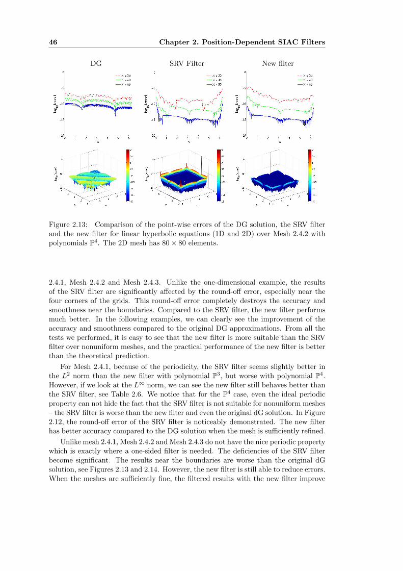
46 Chapter 2. Position-Dependent SIAC Filters
DG SRV Filter New filter
Figure 2.13: Comparison of the point-wise errors of the DG solution, the SRV filterand the new filter for linear hyperbolic equations (1D and 2D) over Mesh 2.4.2 withpolynomials P4. The 2D mesh has 80× 80 elements.
2.4.1, Mesh 2.4.2 and Mesh 2.4.3. Unlike the one-dimensional example, the resultsof the SRV filter are significantly affected by the round-off error, especially near thefour corners of the grids. This round-off error completely destroys the accuracy andsmoothness near the boundaries. Compared to the SRV filter, the new filter performsmuch better. In the following examples, we can clearly see the improvement of theaccuracy and smoothness compared to the original DG approximations. From all thetests we performed, it is easy to see that the new filter is more suitable than the SRVfilter over nonuniform meshes, and the practical performance of the new filter is betterthan the theoretical prediction.
For Mesh 2.4.1, because of the periodicity, the SRV filter seems slightly better inthe L2 norm than the new filter with polynomial P3, but worse with polynomial P4.However, if we look at the L∞ norm, we can see the new filter still behaves better thanthe SRV filter, see Table 2.6. We notice that for the P4 case, even the ideal periodicproperty can not hide the fact that the SRV filter is not suitable for nonuniform meshes– the SRV filter is worse than the new filter and even the original dG solution. In Figure2.12, the round-off error of the SRV filter is noticeably demonstrated. The new filterhas better accuracy compared to the DG solution when the mesh is sufficiently refined.
Unlike mesh 2.4.1, Mesh 2.4.2 and Mesh 2.4.3 do not have the nice periodic propertywhich is exactly where a one-sided filter is needed. The deficiencies of the SRV filterbecome significant. The results near the boundaries are worse than the original dGsolution, see Figures 2.13 and 2.14. However, the new filter is still able to reduce errors.When the meshes are sufficiently fine, the filtered results with the new filter improve
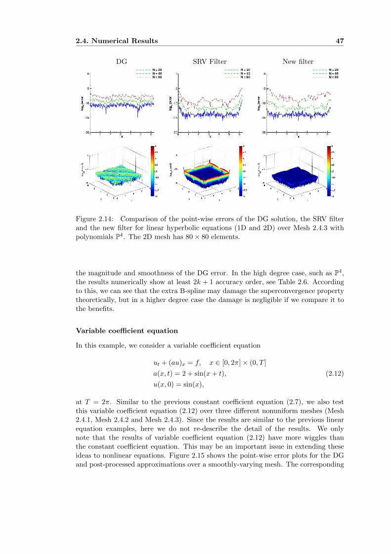
2.4. Numerical Results 47
DG SRV Filter New filter
Figure 2.14: Comparison of the point-wise errors of the DG solution, the SRV filterand the new filter for linear hyperbolic equations (1D and 2D) over Mesh 2.4.3 withpolynomials P4. The 2D mesh has 80× 80 elements.
the magnitude and smoothness of the DG error. In the high degree case, such as P4,the results numerically show at least 2k + 1 accuracy order, see Table 2.6. Accordingto this, we can see that the extra B-spline may damage the superconvergence propertytheoretically, but in a higher degree case the damage is negligible if we compare it tothe benefits.
Variable coefficient equation
In this example, we consider a variable coefficient equation
ut + (au)x = f, x ∈ [0, 2π]× (0, T ]
a(x, t) = 2 + sin(x+ t),
u(x, 0) = sin(x),
(2.12)
at T = 2π. Similar to the previous constant coefficient equation (2.7), we also testthis variable coefficient equation (2.12) over three different nonuniform meshes (Mesh2.4.1, Mesh 2.4.2 and Mesh 2.4.3). Since the results are similar to the previous linearequation examples, here we do not re-describe the detail of the results. We onlynote that the results of variable coefficient equation (2.12) have more wiggles thanthe constant coefficient equation. This may be an important issue in extending theseideas to nonlinear equations. Figure 2.15 shows the point-wise error plots for the DGand post-processed approximations over a smoothly-varying mesh. The corresponding

48 Chapter 2. Position-Dependent SIAC Filters
Table 2.5: L2− and L∞−errors for the DG approximation together with the SRV andthe new filters for linear equation (2.7) over three meshes 2.4.1,2.4.2,2.4.3. A scalingof H = ∆xj along with quadruple precision was used in the computations.
dG Former Filter New FilterMesh L2 error order L∞ error order L2 error order L∞ error order L2 error order L∞ error order
Mesh 2.4.1 P3
20 5.45E-06 – 1.87E-05 – 6.43E-06 – 5.51E-05 – 6.36E-05 – 2.02E-04 –40 3.39E-07 4.01 1.20E-06 3.96 3.11E-07 4.37 3.25E-06 4.09 1.72E-07 8.53 7.62E-07 8.0580 2.12E-08 4.00 7.48E-08 4.01 1.45E-10 11.06 1.81E-09 10.81 2.81E-10 9.26 2.16E-09 8.46
P4
20 1.56E-07 – 5.20E-07 – 5.15E-07 – 4.11E-06 – 1.72E-05 – 5.41E-05 –40 4.83E-09 5.01 1.66E-08 4.97 6.43E-09 6.32 6.56E-08 5.97 2.56E-08 9.39 1.12E-07 8.9180 1.51E-10 5.00 5.22E-10 4.99 1.25E-11 9.01 1.80E-10 8.51 1.15E-11 11.13 7.77E-11 10.50
Mesh 2.4.2 P3
20 3.15E-06 – 1.25E-05 – 1.52E-05 – 1.75E-04 – 1.53E-05 – 7.35E-05 –40 1.96E-07 4.01 8.05E-07 3.96 9.80E-08 7.27 1.50E-06 6.86 3.50E-08 8.77 2.34E-07 8.2980 1.22E-08 4.00 4.97E-08 4.02 2.31E-09 5.40 3.77E-08 5.32 5.63E-11 9.28 8.26E-10 8.15
P4
20 6.25E-08 – 2.67E-07 – 6.79E-07 – 5.38E-06 – 4.45E-06 – 2.13E-05 –40 1.96E-09 5.00 8.77E-09 4.93 2.13E-09 8.32 2.34E-08 7.85 4.12E-09 10.08 2.76E-08 9.5980 6.14E-11 5.00 2.79E-10 4.97 3.03E-11 6.13 5.01E-10 5.54 1.74E-12 11.21 1.59E-11 10.76
Mesh 2.4.3 P3
20 2.49E-06 – 1.06E-05 – 3.35E-05 – 3.61E-04 – 5.64E-06 – 2.90E-05 –40 1.55E-07 4.00 7.46E-07 3.83 7.42E-07 5.50 9.11E-06 5.31 6.23E-09 9.82 3.80E-08 9.5880 1.02E-08 3.93 4.67E-08 4.00 2.46E-08 4.91 4.57E-07 4.32 1.54E-10 5.34 8.71E-10 5.45
P4
20 4.03E-08 – 1.49E-07 – 1.40E-06 – 1.47E-05 – 1.52E-06 – 7.85E-06 –40 1.37E-09 4.88 5.25E-09 4.83 1.42E-08 6.63 1.78E-07 6.36 3.20E-10 12.21 1.98E-09 11.9580 4.40E-11 4.96 1.70E-10 4.95 4.03E-10 5.13 7.93E-09 4.49 3.68E-13 9.77 3.95E-12 8.97
errors are given in Table 2.7. The results are similar to the linear examples, the twofilters perform similarly, with the new filter being more computationally efficient.
DG SRV Filter New filter
Figure 2.15: Comparison of the point-wise errors of the DG solution, the SRV fil-ter and the new filter for variable coefficient equation (2.12) over Mesh 2.4.1 withpolynomials P4.
For the smooth polynomial mesh 2.4.2, we show the point-wise error plots in Figure2.16. The corresponding errors are given in Table 2.7. In this example we see that thenew filter behaves better at the boundaries than the SRV filter. This may be due to

2.4. Numerical Results 49
Table 2.6: L2− and L∞−errors for the DG approximation together with the SRV andnew filters for 2D linear equation (2.8) using polynomials of degree k = 3, 4 over threemeshes: Mesh 2.4.1, Mesh 2.4.2 and Mesh 2.4.3.
DG SRV Filter New FilterMesh L2 error order L∞ error order L2 error order L∞ error order L2 error order L∞ error order
Mesh 2.4.1 P3
20× 20 8.74E-06 – 5.39E-05 – 6.94E-06 – 1.10E-04 – 6.71E-05 – 4.04E-04 –40× 40 5.45E-07 4.00 3.39E-06 4.00 3.68E-07 4.24 6.49E-06 4.08 2.09E-07 8.33 1.66E-06 7.9380× 80 3.40E-08 4.00 2.06E-07 4.03 1.50E-10 11.76 9.01E-09 9.49 7.33E-10 8.16 7.76E-09 8.92
P4
20× 20 1.93E-07 – 1.05E-06 – 9.25E-07 – 8.56E-06 – 3.26E-05 – 1.12E-04 –40× 40 6.00E-09 5.01 3.32E-08 4.98 3.38E-08 4.77 4.17E-06 1.04 2.67E-08 10.25 2.31E-07 8.9280× 80 1.88E-10 5.00 1.04E-09 5.00 2.07E-08 0.71 9.13E-06 -1.13 1.90E-11 10.46 1.61E-10 10.49
Mesh 2.4.2 P3
20× 20 4.56E-06 – 3.03E-05 – 1.55E-05 – 3.49E-04 – 1.59E-05 – 1.38E-04 –40× 40 2.85E-07 4.00 1.92E-06 3.98 1.23E-07 6.98 3.04E-06 6.84 4.67E-08 8.41 5.14E-07 8.6780× 80 1.78E-08 4.00 1.20E-07 4.00 3.35E-09 5.20 8.01E-08 5.25 2.43E-10 7.59 4.61E-09 6.80
P4
20× 20 8.48E-08 – 3.27E-07 – 1.38E-06 – 1.48E-05 – 5.92E-06 – 3.27E-05 –40× 40 2.65E-09 5.00 1.74E-08 4.92 3.21E-08 5.43 4.99E-06 1.57 4.65E-09 10.30 5.79E-08 9.1480× 80 8.31E-11 5.00 5.58E-10 4.96 2.51E-08 0.35 6.88E-06 -0.46 3.29E-12 10.46 3.49E-11 10.27
Mesh 2.4.3 P3
20× 20 3.47E-06 – 2.16E-05 – 3.46E-05 – 6.43E-04 – 3.90E-06 – 3.83E-05 –40× 40 2.23E-07 3.96 1.52E-06 3.83 1.90E-06 4.19 3.59E-05 4.16 1.28E-08 8.25 1.25E-07 8.2680× 80 1.41E-08 3.98 9.65E-08 3.98 9.94E-08 4.26 2.71E-06 3.73 2.97E-10 5.43 3.88E-09 5.01
P4
20× 20 5.83E-08 – 2.84E-07 – 3.06E-06 – 5.19E-05 – 1.06E-06 – 8.87E-05 –40× 40 1.90E-09 4.94 1.04E-08 4.77 2.64E-08 6.86 2.64E-06 4.30 7.80E-10 10.41 1.01E-08 9.7880× 80 6.06E-11 4.97 3.48E-10 4.90 1.46E-08 0.85 7.09E-06 -1.43 6.60E-13 10.20 7.85E-12 10.33
the more compact filter support size.
DG SRV Filter New filter
Figure 2.16: Comparison of the point-wise errors of the DG solution, the SRV fil-ter and the new filter for variable coefficient equation (2.12) over Mesh 2.4.2 withpolynomials P4.
Finally, we test the variable coefficient equation (2.12) over a randomly-varyingmesh 2.4.3. Similar to the linear examples, the point-wise errors plots, Figure 2.17,show more oscillations than smoothly-varying mesh examples. We again see the newfilter has better errors at the boundaries than the SRV filter.
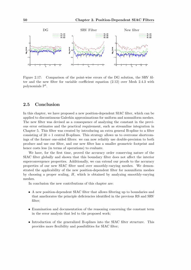
50 Chapter 2. Position-Dependent SIAC Filters
DG SRV Filter New filter
Figure 2.17: Comparison of the point-wise errors of the DG solution, the SRV fil-ter and the new filter for variable coefficient equation (2.12) over Mesh 2.4.3 withpolynomials P4.
2.5 Conclusion
In this chapter, we have proposed a new position-dependent SIAC filter, which can beapplied to discontinuous Galerkin approximations for uniform and nonuniform meshes.The new filter was devised as a consequence of analyzing the constant in the previ-ous error estimates and the practical requirement, such as streamline integration inChapter 5. This filter was created by introducing an extra general B-spline to a filterconsisting of 2k + 1 central B-splines. This strategy allows us to overcome shortcom-ings of the former one-sided filters: we can now reliably use double-precision to bothproduce and use our filter, and our new filter has a smaller geometric footprint andhence costs less (in terms of operations) to evaluate.
We have, for the first time, proved the accuracy order conserving nature of theSIAC filter globally and shown that this boundary filter does not affect the interiorsuperconvergence properties. Additionally, we can extend our proofs to the accuracyproperties of our new SIAC filter used over smoothly-varying meshes. We demon-strated the applicability of the new position-dependent filter for nonuniform meshesby choosing a proper scaling, H, which is obtained by analyzing smoothly-varyingmeshes.
In conclusion the new contributions of this chapter are:
• A new position-dependent SIAC filter that allows filtering up to boundaries andthat ameliorates the principle deficiencies identified in the previous RS and SRVfilter;
• Examination and documentation of the reasoning concerning the constant termin the error analysis that led to the proposed work;
• Introduction of the generalized B-splines into the SIAC filter structure. Thisprovides more flexibility and possibilities for SIAC filter;

2.5. Conclusion 51
Table 2.7: L2− and L∞−errors for the DG approximation together with the SRV andthe new filters for variable coefficient equation (2.12) over the three meshes.
DG SRV Filter New FilterMesh L2 error order L∞ error order L2 error order L∞ error order L2 error order L∞ error order
Mesh 2.4.1 P3
20 5.54E-06 – 1.93E-05 – 4.40E-06 – 3.66E-05 – 6.36E-05 – 2.02E-04 –40 3.41E-07 4.02 1.21E-06 4.00 3.14E-07 3.81 3.25E-06 3.49 1.72E-07 8.53 7.61E-07 8.0580 2.12E-08 4.01 7.50E-08 4.01 1.45E-10 11.08 1.81E-09 10.81 2.78E-10 9.27 2.05E-09 8.53
P4
20 1.62E-07 – 5.69E-07 – 1.89E-05 – 1.44E-04 – 1.72E-05 – 5.41E-05 –40 4.95E-09 5.03 1.77E-08 5.00 5.74E-09 11.68 5.82E-08 11.28 2.56E-08 9.39 1.12E-07 8.9180 1.53E-10 5.01 5.48E-10 5.02 1.26E-11 8.83 1.76E-10 8.37 1.16E-11 11.11 7.26E-11 10.59
Mesh 2.4.2 P3
20 3.15E-06 – 1.27E-05 – 2.70E-05 – 3.05E-04 – 1.53E-05 – 7.36E-05 –40 1.96E-07 4.01 8.06E-07 3.98 1.31E-07 7.69 1.54E-06 7.62 3.55E-08 8.75 2.38E-07 8.2880 1.22E-08 4.00 4.98E-08 4.02 7.51E-09 4.13 1.27E-07 3.60 6.25E-11 9.15 7.84E-10 8.24
P4
20 6.40E-08 – 2.82E-07 – 2.95E-06 – 2.42E-05 – 4.45E-06 – 2.13E-05 –40 1.98E-09 5.01 8.94E-09 4.98 6.84E-07 2.11 1.12E-05 1.10 4.12E-09 10.08 2.76E-08 9.6080 6.18E-11 5.00 2.80E-10 5.00 1.51E-09 8.83 3.50E-08 8.33 1.59E-12 11.34 1.55E-11 10.80
Mesh 2.4.3 P3
20 2.49E-06 – 9.61E-06 – 1.11E-04 – 8.98E-04 – 5.63E-06 – 2.90E-05 –40 1.56E-07 4.00 7.18E-07 3.74 2.12E-06 5.71 2.55E-05 5.14 7.96E-09 9.47 4.31E-08 9.3980 1.02E-08 3.93 4.72E-08 3.93 5.91E-08 5.17 1.06E-06 4.59 3.15E-10 4.66 1.91E-09 4.50
P4
20 4.07E-08 – 1.56E-07 – 2.45E-05 – 1.96E-04 – 1.52E-06 – 7.85E-06 –40 1.37E-09 4.89 5.31E-09 4.87 4.48E-07 5.77 6.18E-06 4.99 2.98E-10 12.31 1.79E-09 12.0980 4.41E-11 4.96 1.73E-10 4.94 1.26E-09 8.48 1.91E-08 8.33 2.64E-12 6.82 2.19E-11 6.35
• Demonstration that the filtered approximation is always superconvergent in theuniform mesh linear polynomial case;
• Theoretical proof of the equivalence of smoothly-varying meshes and uniformmeshes, in the view of accuracy order;
• Application of the scaled new filter to both smoothly-varying and nonuniform(random) meshes, for which cases we still see significant improvement in thesmoothness and an error reduction of the original DG solution, although fullsuperconvergence is not always achieved.

3Derivative SIAC Filters
3.1 Introduction
In many cases, one can argue persuasively that the changes in values of a functionare often more import than the values themselves, such as exhibited by streamlineintegration of fields. Therefore, an accurate derivative approximation is often requiredin many areas such as biomechanics, optimization, chemistry and visualization appli-cations. However, computing derivatives of discontinuous Galerkin approximations ischallenging because the DG solution only has weak continuity at element boundaries.This means that the strong form of derivatives for a DG solution technically do nothold at element boundaries, and computing the derivative directly does not alwaysproduce accurate results. For example, naive and careless use of the derivatives ofthe discontinuous Galerkin solution directly to streamline integration can produce in-consistent results with the exact solution [61]. Once derivatives are needed near theboundaries, the difficulty increases since the solution often has less regularity in thoseregions.
In order to obtain accurate approximations for the derivatives of DG solutions,one can use the symmetric derivative SIAC filter we introduced in Chapter 1. Asits name implies, the SIAC filter can increase the smoothness of DG solutions, andthis smoothness-increasing property helps to enhance the accuracy of derivatives ofDG solutions. With the symmetric derivative filter, the accuracy order of the filteredDG solution can be improved from k + 1 to 2k + 1 regardless of the derivative order.However, previous investigations of derivative filtering have two major limitations: therequirement of uniform meshes and periodic boundary conditions.
In this chapter, we focus on overcoming these two limitations. We propose position-dependent derivative filters to approximate the derivatives of the DG solution overnonuniform meshes and near boundaries. Our main contributions are:
Nonuniform Meshes. Filtering over nonuniform meshes has always been a sig-nificant challenge for SIAC filtering because the 2k + 1 accuracy order is no longerguaranteed in general. Most of previous work for nonuniform meshes (such as [30, 55])only considered a particular family of nonuniform meshes, smoothly-varying meshes.Among these works, only [55] mentioned derivatives over nonuniform meshes. It dis-
53

54 Chapter 3. Derivative SIAC Filters
cussed the challenges of derivative filtering over nonuniform meshes and presentedpreliminary results concerning smooth-varying meshes. In this chapter, we propose amethod for arbitrary nonuniform meshes: using the scaling H = hµ for filtering overnonuniform meshes. This does not guarantee that the derivative filtering improves thederivatives of DG solutions to accuracy order of 2k + 1, but we prove that a higherconvergence rate (compared to DG solution) is still obtained. Further, the numericalexamples suggest that the accuracy is improved once the mesh is sufficiently refined.
Boundaries. First, we point out that previously derivative filters could not beused near boundaries except for periodic meshes. Without considering derivatives, asmentioned in the previous chapters there are three existing position-dependent filtersthat can be used to handle boundary regions. The first one is the RS filter (1.12)introduced by Ryan and Shu [57]; the second one is the SRV filter (1.14) given by vanSlingerland, Ryan and Vuik [65]; lastly, the newly defined postion-dependent filter dis-cussed in Chapter 2, which we simply refer to the new filter in this chapter. The RS andSRV filters, [57, 65], are constructed by only using central B-splines. They show goodperformance over uniform meshes. The new filter introduced in Chapter 2 is aimed atnonuniform meshes. It uses 2k+1 central B-splines and an extra general B-spline. Theresults in Chapter 2 suggest that adding the extra general B-spline improves the perfor-mance of the position-dependent filter over nonuniform meshes compared to using onlycentral B-splines. In this chapter, we extend the SRV position-dependent filter [65]and the new position-dependent filter in Chapter 2 to position-dependent derivative fil-ters. Then, we discuss the advantages and disadvantages of these position-dependentderivative filters over uniform and nonuniform meshes. For nonuniform meshes, weprove that by using the position-dependent derivative filtering, the convergence rate ofderivatives of the DG solution can be improved. Numerical comparisons over uniformand nonuniform meshes also demonstrate that the derivative filtered solutions are moreaccurate than the derivatives of DG approximations.
3.2 Symmetric and One-Sided Derivative Filters
Smoothness-Increasing Accuracy-Conserving filtering is named after its improvementof the smoothness of the filtered approximation. Using the filter in equation (1.6), thefiltered solution is a Ck−1 function. One can see that the smoothness is significantlyimproved from the original weakly continuous DG solution. By taking advantage ofthe improved smoothness, we can obtain better derivative approximations.
3.2.1 Derivative Filters over Nonuniform Meshes
The symmetric derivative filter over uniform meshes was introduced in [56, 62]. In thesepapers, the authors identified two ways to calculate the derivatives. The first methodis a direct calculation of the derivatives of the filtered solution (1.5). The convergencerate of the filtered solution is higher than the derivatives of the DG approximationitself, but the accuracy order decreases and oscillations in the error increase with eachsuccessive derivative. The second method is employed to maintain a fixed accuracyorder regardless of the derivative order. To calculate the αth derivative of the DG

3.2. Symmetric and One-Sided Derivative Filters 55
approximation without losing any accuracy order, we have to use higher-order centralB-splines to construct the filter. We remind the reader that
∂αxu?h = ∂αx
(K
(2k+1,k+1+α)h ? uh
)=
(dα
dxαK
(2k+1,k+1+α)h
)? uh
=(∂αh K
(2k+1,k+1,α)h
)? uh = K
(2k+1,k+1,α)h ? ∂αhuh,
(3.1)
where the symmetric derivative filter is
K(2k+1,k+1+α)(x) =
2k∑γ=0
c(2k+1,k+1+α)γ ψ(k+1+α)(x+ k − γ). (3.2)
For uniform meshes, [56] showed the filtered solution (3.1) has superconvergence rateof 2k + 1 regardless of the derivative order α.
‖∂αxu− ∂αxu?h‖0 ∼ O(h2k+1).
Unfortunately, these methods are limited to uniform meshes. For nonuniform meshes,applying the SIAC filter becomes complicated, and the derivative SIAC filter is evenmore difficult. If we naively apply the same derivative filter (3.2) over nonuniformmeshes, we will lose accuracy from O(h2k+1) to O(hk+1−α) since over nonuniformmeshes the divided differences of the DG solution no longer have the superconvergenceproperty, see the next chapter for details.
A brief introductory description of symmetric derivative filtering over nonuniformmeshes can be found in [55]. It discusses the challenges of symmetric derivative filteringover nonuniform meshes and gives preliminary results for smoothly-varying meshes (anaffine mapping of a uniform mesh [30]). Also, in Chapter 2, we have already providedthe error estimates for the filtered solutions over smoothly-varying meshes. From thoseprevious results, we can see that the key to SIAC filtering over nonuniform meshes is:the filter scaling H and the divided differences of the DG solution. To begin the study,we first present an error estimate for the divided differences of the DG solution overgeneral nonuniform meshes with a general scaling H.
Lemma 3.2.1. Under the same conditions in Theorem 1.2.1, let uh be the DG approx-imation over a nonuniform mesh. Denote Ω0 ⊂⊂ Ω1 ⊂⊂ Ω, ` ≥ k + 1. The negativeorder norm estimate of u− uh satisfies,
‖(u− uh)(T )‖−`,Ω1 ≤ Ch2k+1,
and‖∂αH(u− uh)(T )‖−`,Ω0 ≤ Cαh
2k+1H−|α|,
where α = (α1, . . . , αd) is an arbitrary multi-index and H is the scaling of the divideddifference operator ∂αH .
Proof. The proof of the negative order norm estimate was given in [25] and the divideddifference estimate was presented as a hypotheses. The proof is trivial and thereforewe only give a proof for d = 1 case.

56 Chapter 3. Derivative SIAC Filters
Set Ω0 such that Ω0+[− |α|H
2 , |α|H2
]⊂ Ω1. Consider the first divided difference, by
the definition of the negative order norm, we have
‖∂H(u− uh)‖−`,Ω0
= supΦ∈C∞
0 (Ω0)
(((u− uh)(x+ H
2 ),Φ)−((u− uh)(x− H
2 ),Φ)
H‖Φ‖`,Ω0
),
≤ supΦ∈C∞
0 (Ω0)
((u− uh)(x+ H
2 ),Φ)
H‖Φ‖`,Ω0
+ supΦ∈C∞
0 (Ω0)
((u− uh)(x− H
2 ),Φ)
H‖Φ‖`,Ω0
,
≤ 2
H‖u− uh‖−`,Ω1 .
By induction, we have
‖∂αH(u− uh)(T )‖−`,Ω0 ≤ Cαh2k+1H−|α|,
where Cα = 2|α|C. The proof is similar for d > 1 case.
Lemma 3.2.1 demonstrates the optimal accuracy order estimation of the divideddifferences of the DG approximation in the sense that the nonuniform mesh is arbi-trary [25, 51]. Based on Lemma 3.2.1, we can give the following error estimations fornonuniform meshes.
Theorem 3.2.2. Under the same conditions as in Lemma 3.2.1, let K(r+1,k+1+α) bethe symmetric derivative filter given in (3.2). Denote
Ω0 + 2supp(K(r+1,k+1+α)H ) ⊂⊂ Ω1 ⊂⊂ Ω.
Then, for general nonuniform meshes, we have
‖∂αxu− ∂αx(K
(r+1,k+1+α)H ? uh
)‖0,Ω0 ≤ Ch
r+1r+k+2+α
(2k+1),
where H = hµ and µ = 2k+1r+k+2+α .
Proof. Set Ω1/2 such that
Ω0 + supp(K(r+1,k+1+α)H ) ⊂ Ω1/2, Ω1/2 + supp(K
(r+1,k+1+α)H ) ⊂ Ω1.
By applying Lemma 1.2.2 and Lemma 3.2.1, we have∥∥∥∂αxu− ∂αx (K(r+1,k+1+α)H ? uh
)∥∥∥0,Ω0
≤∥∥∥∂αxu−K(r+1,k+1+α)
H ? ∂αxu∥∥∥0,Ω0
+∥∥∥∂αx (K(r+1,k+1+α)
H ? (u− uh))∥∥∥
0,Ω0
≤C0Hr+1 + C1
∑|β|≤k+1
∥∥∥∂α+βx
(K
(r+1,k+1+α)H ? (u− uh)
)∥∥∥−(k+1),Ω1/2
=C0Hr+1 + C1
∑|β|≤k+1
∥∥∥(K(r+1,k+1−β,α+β)H ? ∂α+β
H (u− uh))∥∥∥
−(k+1),Ω1/2
=C0Hr+1 + C1
∑|β|≤k+1
∥∥∥K(r+1,k+1−β,α+β)H
∥∥∥L1
∥∥∥∂α+βH (u− uh)
∥∥∥−(k+1),Ω1
≤C0Hr+1 + C2h
2k+1H−(k+1+α),

3.2. Symmetric and One-Sided Derivative Filters 57
Let the scaling H = hµ such that
Hr+1 = h2k+1H−(k+1+α).
We then have that µ = 2k+1r+k+2+α and∥∥∥∂αxu− ∂αx (K(r+1,k+1+α)
H ? uh
)∥∥∥0,Ω0
≤ Chr+1
r+k+2+α(2k+1).
Remark 3.2.1 (Discussion of the Number of B-splines). The filter given in (3.2) uses(r + 1) B-splines. Theorem 3.2.2 implies that by increasing the value of r, one canincrease the value of r+1
r+k+2+α , and then approximate the superconvergence rate 2k+1as close as we want and regardless of the derivative order α. However, increasing thevalue of r presents a serious inconvenience for computational implementation. Forexample, while r 2k, a multi-precision package is required during the computationprocess, see Chapter 2. Another disadvantage is that the support size of the filter,(r+k+1+α)hµ, increases with r [25]. The increased support size means the convolutioninvolves more DG elements and that the computational cost is increased as well. Fornonderivative filtering, we usually keep r = 2k. There is another consideration forderivative filtering. We notice that the accuracy order decreases with the derivativeorder α if we keep r = 2k. One solution is to eliminate the negative effect of thederivative order α is to use r = 2(k + α) instead of r = 2k. However, our experienceshows that the benefit of using r = 2(k+α) is limited. It slightly improves the accuracyand smoothness, but increases the computational cost. In this chapter, we will focuson using r = 2k for nonuniform meshes.
3.2.2 Position-Dependent Derivative Filters
For convenience, we use symbol ` instead of k + 1 + α in following section.
Derivative RS Filter
To begin, we first introduce how to extend the first one-sided filter, the RS filter, tothe derivative RS filter.
Since the RS filter is an integer shifted symmetric filter, we can easily extend itto the derivative RS filter by increasing the order of B-splines and then modifying theshift function.
K(2k+1,`)(x) =2k∑γ=0
c(2k+1,`)γ ψ(`) (x− xγ(x)) , (3.3)
where xγ depends on the location of the evaluation point x and is given by
xγ(x) = −k + γ + [λ](x),
with discrete shift
[λ](x) =
min0,−2k+`
2 + b x−xLh c, x ∈ [xL,
xL+xR2 ),
max0, 2k+`2 + d x−xR
h e, x ∈ [xL+xR2 , xR].

58 Chapter 3. Derivative SIAC Filters
Here xL and xR are the left and right boundaries, respectively. An example of thederivative RS filter (for the left boundary) with k = 2 is given in Figure 3.1.
α = 0
−10 −8 −6 −4 −2 0−20
−10
0
10
20
30α = 1
−10 −8 −6 −4 −2 0−20
−10
0
10
20
30α = 2
−10 −8 −6 −4 −2 0−20
−10
0
10
20
30
Figure 3.1: Derivative RS filter (3.3) with k = 2.
Derivative SRV Filter
The SRV filter has a similar structure as the RS filter, without the discrete shift. Byusing a similar method, we can extend it to the derivative SRV filter. This is given as
K(4k+1,`)(x) =
4k∑γ=0
c(4k+1,`)γ ψ(`) (x− xγ(x)) , (3.4)
where xγ depends on the location of the evaluation point x and is given by
xγ(x) = −2k + γ + λ(x).
We adjust the shift function λ(x) (1.15) by
λ(x) =
min0,−4k+`
2 + x−xLh , x ∈ [xL,
xL+xR2 ),
max0, 4k+`2 +
x−xright
h , x ∈ [xL+xR2 , xR].
Here xL and xR are the left and right boundaries, respectively. An example of thederivative SRV filter (for the left boundary) with k = 2 is given in Figure 3.2.
Remark 3.2.2. As mentioned in Chapter 1, the main difference between the RS filterand the SRV filter is the number of B-splines.
Remark 3.2.3. The theoretical analysis of the derivative RS and SRV filters remainsthe same as in Theorem 3.2.2. Unlike the derivative RS filter and the symmetric
derivative filter, the derivative SRV filter has a scaling H = h2k+1
5k+2+α , which is muchlarger than the scaling of the symmetric derivative filter (or the derivative RS filter),
H = h2k+1
3k+2+α .

3.2. Symmetric and One-Sided Derivative Filters 59
α = 0
−14−12−10 −8 −6 −4 −2 0−400
−200
0
200
400
600α = 1
−14−12−10 −8 −6 −4 −2 0−400
−200
0
200
400
600α = 2
−14−12−10 −8 −6 −4 −2 0−400
−200
0
200
400
600
Figure 3.2: Derivative SRV filter (3.4) with k = 2.
New Position-Dependent Derivative Filter
For the new position-dependent filter introduced in Chapter 2, we need to shift the2k + 1 central B-splines and then change the extra general B-spline according to thederivative order α. To complete these changes, we have to change the knot sequence ofthe original new position-dependent filter, which is used only for the DG approximationuh without derivatives. For the new position-dependent derivative filter near the leftboundary (similar for the right boundary), we need to redistribute the knots in theknot matrix T to meet the derivative requirement by
T (γ, j) =
−2k − `+ j + γ + x−xL
h , 0 ≤ γ ≤ 2k, 0 ≤ j ≤ `;x−xL
h +minj − α, 0, γ = 2k + 1, 0 ≤ j ≤ `. (3.5)
The position-dependent derivative filter is then given by
K(2k+1,`)T (x) =
2k∑γ=0
c(2k+1,`)γ ψ
(`)T(γ)(x)︸ ︷︷ ︸
2k + 1 central B-splines
+ c(2k+1,`)2k+1 ψ
(`)T(2k+1)︸ ︷︷ ︸
General B-spline
. (3.6)
We note that in formula (3.5), if we keep the order of B-splines as k + 1, then whenα > k the general B-spline added at the boundary will reduce to the central B-splineand then the purpose of adding a special B-spline at the boundary fails. It is necessaryto use B-splines of order ` = k + 1 + α instead of k + 1 when α > k. We notethat the new position-dependent derivative filter allows us to approximate arbitraryorder derivatives near boundaries theoretically. For example, Figure 3.3 shows the newposition-dependent derivative filters with k = 2 for the first and second derivatives atthe left boundary. Compared to the derivative RS filter (3.3), the derivative SRV filter(3.4), the new position-dependent derivative filter clearly has reduced support andmagnitude (range from −400 to 600 versus −4 to 6).
Theorem 3.2.3. Under the same conditions as in Lemma 3.2.1, let K(2k+1,`)T be the
new position-dependent derivative filter (3.6). We have∥∥∥∂αxu− ∂αx (K(2k+1,`)HT ? uh
)∥∥∥0,Ω0
≤ Chµ(2k+2),
where H = hµ, µ = 2k+13k+3+α .
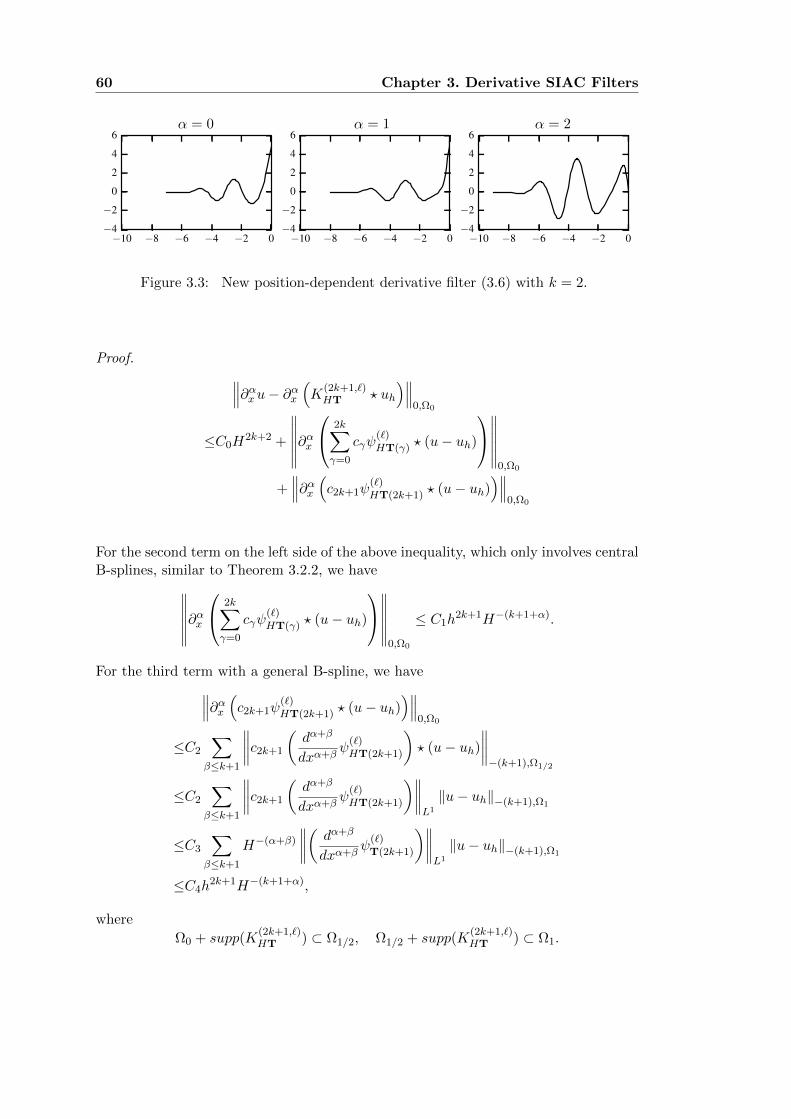
60 Chapter 3. Derivative SIAC Filters
α = 0
−10 −8 −6 −4 −2 0−4
−2
0
2
4
6α = 1
−10 −8 −6 −4 −2 0−4
−2
0
2
4
6α = 2
−10 −8 −6 −4 −2 0−4
−2
0
2
4
6
Figure 3.3: New position-dependent derivative filter (3.6) with k = 2.
Proof. ∥∥∥∂αxu− ∂αx (K(2k+1,`)HT ? uh
)∥∥∥0,Ω0
≤C0H2k+2 +
∥∥∥∥∥∥∂αx 2k∑
γ=0
cγψ(`)HT(γ) ? (u− uh)
∥∥∥∥∥∥0,Ω0
+∥∥∥∂αx (c2k+1ψ
(`)HT(2k+1) ? (u− uh)
)∥∥∥0,Ω0
For the second term on the left side of the above inequality, which only involves centralB-splines, similar to Theorem 3.2.2, we have∥∥∥∥∥∥∂αx
2k∑γ=0
cγψ(`)HT(γ) ? (u− uh)
∥∥∥∥∥∥0,Ω0
≤ C1h2k+1H−(k+1+α).
For the third term with a general B-spline, we have∥∥∥∂αx (c2k+1ψ(`)HT(2k+1) ? (u− uh)
)∥∥∥0,Ω0
≤C2
∑β≤k+1
∥∥∥∥c2k+1
(dα+β
dxα+βψ(`)HT(2k+1)
)? (u− uh)
∥∥∥∥−(k+1),Ω1/2
≤C2
∑β≤k+1
∥∥∥∥c2k+1
(dα+β
dxα+βψ(`)HT(2k+1)
)∥∥∥∥L1
‖u− uh‖−(k+1),Ω1
≤C3
∑β≤k+1
H−(α+β)
∥∥∥∥( dα+β
dxα+βψ(`)T(2k+1)
)∥∥∥∥L1
‖u− uh‖−(k+1),Ω1
≤C4h2k+1H−(k+1+α),
where
Ω0 + supp(K(2k+1,`)HT ) ⊂ Ω1/2, Ω1/2 + supp(K
(2k+1,`)HT ) ⊂ Ω1.

3.2. Symmetric and One-Sided Derivative Filters 61
Then, we have∥∥∥∂αxu− ∂αx (K(2k+1,`)HT ? uh
)∥∥∥0,Ω0
≤ C0H2k+2 + C5h
2k+1H−(k+1+α).
Similar to the symmetric filter case in Theorem 3.2.2, we require that the scaling Hsatisfies H2k+2 = h2k+1H−(k+1+α) and finally, we have∥∥∥∂αxu− ∂αx (K(2k+1,`)
HT ? uh
)∥∥∥0,Ω0
≤ Chµ(2k+2),
where H = hµ and µ = 2k+13k+3+α .
3.2.3 Computational Considerations
Theorem 3.2.2 and Theorem 3.2.3 give convergence rates of the symmetric and position-dependent derivative filters, respectively. One can easily verify that the convergencerates are better than calculating the derivatives of DG approximation directly, k+1−α.Now, let us consider the computational efficiency of the one-sided derivative filters.
Support Size of the Filters
As mentioned before, the support size of the filters is one import component whichaffects the computational cost of using the filters. For nonuniform meshes, Theorem3.2.2 and Theorem 3.2.3 require the scaling has the form H = hµ. For conveniencewe let the degree k → ∞. Then, the symmetric derivative filter, the derivative RSfilter, and the new derivative filters have the same scaling H = h2/3 and support size(3k + 1 + α)h2/3; the derivative SRV filter has a much larger scaling H = h2/5 andsupport size (5k+1+α)h2/5. It is obvious that the SRV filter has a significantly largersupport size compared to other filters, especially when h is very small (a very finemesh). It follows that the computational cost of using the new filter is much cheaperthan using other filters.
However, we notice that the scaling H = hµ is still quite large compared to h. Thelarge support usually has negative effects on the accuracy over coarse meshes. Let thedomain be Ω = [0, 1] and h = 1/N , where N is the number of elements. In orderto guarantee the conclusions in Theorem 3.2.2 and Theorem 3.2.3, we must choose Nlarge enough so that the support size of the filters is less than the domain size, whichrequires
(r + k + α+ 1)hµ ≤ 1 =⇒ N ≥ (r + k + α+ 1)1/µ,
here r = 2k for the symmetric and new position-dependent derivative filters and r = 4kfor the derivative SRV filter. Table 3.1 gives the minimum number of elements fordifferent filters. We note that for the SRV filter, the required number of elements isalways too large, this is one important reason that the SRV filter performs poorly overnonuniform meshes. Once N is smaller than the minimum requirement given in Table3.1, we have to rescale the filter by using scaling H = 1/(r+ k+α+1). However, thisrescaling technique normally has negative effects on the accuracy order.

62 Chapter 3. Derivative SIAC Filters
Table 3.1: The minimum number of elements according to the derivative order α.Here, N1 is used for the symmetric and new position-dependent derivative filters andN2 is used for the derivative SRV filter.
N1
N2α = 0 α = 1 α = 2 α = 3 α = 4 α = 5
k = 18
89 12130 15
182 19243 23
317 27402
k = 219
402 23499 27
610 32734 37
872 421024
k = 332
1024 371192 42
1375 471574 53
1789 592021
Order of the B-splines
Although we know that the new derivative filter is already much more efficient than thederivative SRV filter, it still less efficient compared to the filters for uniform meshes(scaling H = O(h)). It is understandable that one needs more effort to deal withnonuniform meshes compared to uniform meshes, but we still want to reduce thecomputational cost if possible. Based on the current support size, (3k + 1 + α)hµ
with µ = 2/3, there are two directions to reduce the support size. The first one is toincrease the value of µ. This idea will lead to a new analysis about the relation of µand the structure of nonuniform meshes. This will be discussed in the next chapter.The second thought is to reduce the order of the B-splines. One can use only the orderk + 1 for derivatives of order ≤ k. Then the support size is reduced to (3k + 1)h2/3.Although the improvement is not too much and has a risk to reduce the accuracy whenα ' k.
Remark 3.2.4. Reducing the support size of the filters has another benefit besidesreducing the computational cost. Once the support size of the filters is reduced, onecan apply the symmetric filter in a larger region, which enhances the performance.
3.3 Numerical Results
In the previous section, we proposed three position-dependent derivative filters andinvestigated how to choose the proper scaling of the filters over nonuniform meshes.We also proved that the filtered solutions have better accuracy order and smoothnesscompared to the original DG approximations regardless of the derivative order α. Wenow turn to the numerical examples for the position-dependent derivative filters. Theaims of this section are:
1. Testing the position-dependent derivative filters (the SRV and new filter) foruniform meshes, which has never been done before;
2. Applying the symmetric and position-dependent derivative filters over differentnonuniform meshes;
3. Comparing the derivative filters with different order B-splines. For convenience,we introduce the following notation:
3.3. Numerical Results 63
• the derivative of the filtered solution, ∂αxu?h. This filtered solution uses the
standard filter and then takes the derivative.
• the filtered derivative,(∂αHKH
)?uh, which uses the higher order derivative
filter K(r+1,k+1+α)H for filtering the DG solution.
Remark 3.3.1. Here, we do not present the results of using the derivative RS filteras it is very similar to the derivative SRV filter. Their difference is the number ofB-splines, and we will discuss the effects of the number of B-splines in the next chap-ter. We note that for the following uniform mesh examples, the SRV filter has betterperformance compared to the RS filter.
We note that the DG approximation makes sense only when α ≤ k. In addition, thederivative of the filtered solution ∂αxu
?h loses the wanted accuracy order when α > k
(u?h = Kr+1,k+1H ?uh is a Ck−1 function only). Therefore, we mainly present comparison
examples with α ≤ k situation in this section. When α > k, we only present the
results of the filtered derivative(∂αHKH
)? uh, and we point out that the filtered
solution(∂αHKH
)? uh has a theoretical meaning for an arbitrary α, but the accuracy
deteriorates with each successive derivative. However, we also note that once α > k,the nonuniform meshes have to be sufficiently refined in order to see the accuracyimprovement. Because of these reasons, we only present α = k+1 case for nonuniformmeshes. Also, since the symmetric derivative filter is applied in the interior region ofeach example, we do not present it separately.
3.3.1 Uniform Mesh
Before approaching nonuniform meshes, we first apply the position-dependent deriva-tive filters over uniform meshes. Here we present results of using both the SRV filterand the new filter since each of them has an advantage over uniform meshes that weaddress in the following examples. Consider a linear convection equation
ut + ux = 0, x ∈ [0, 1], (3.7)
u(x, 0) = sin(2πx),
at time T = 1 with periodic boundary conditions. For uniform meshes, we can also usescaling H = hµ and obtain results as Theorems 3.2.2 and 3.2.3 described. However,according to the analysis in [25, 65], in order to maximize the benefits of using centralB-splines over uniform meshes, we choose the uniform mesh size, h, as the filter scaling.Here, we compare the derivatives of the DG approximation, the filtered solutions (theSRV and new filter) with using B-splines of order k+1+α (Table 3.2 and Figure 3.4)and using B-splines of order k + 1 (Table 3.3 and Figure 3.5). From the tables, we
can see that the filtered solutions(∂αHKH
)?uh and ∂αx (KH ?uh) have better accuracy
compared to the original DG solutions. Generally speaking, ∂αx (KH ? uh) is better for
high order derivatives and(∂αHKH
)?uh performs well for the first derivative. Further
comparison of these two methods will list in the end of the section.

64 Chapter 3. Derivative SIAC Filters
With the scaling H = h, the SRV filter clearly has an advantage for uniformmeshes. Because the SRV is constructed using only central B-splines, and was provento have 2k + 1 accuracy order regardless of the derivative order α for linear equationsover uniform meshes in [57]. In Tables 3.2 and 3.3, the SRV filter shows smaller errorscompared to the new filter near the boundaries, especially when α is large. For thenew position-dependent derivative filter, we notice that the filtered solutions only haveaccuracy of order k+1−α in Tables 3.2 and 3.3. This is because we use a scaling H = hinstead of a scalingH = hµ as in Theorem 3.2.3. We note that if using a multi-precisionpackage is acceptable, then the SRV filter is more advantageous for the accuracy order.However, if only double precision is available during computation (for example, GPUcomputing), then in order to avoid round-off errors, the new position-dependent filteris a better choice, see Chapter 2. However, when α > k, the optimal choice is still theSRV filter with B-splines of order k + 1 + α because only this filter does not lose theaccuracy with each successive derivative.
We note that the derivative of filtered solution ∂αx (KH ? uh) also performs wellnear boundaries for uniform meshes, especially for the new position-dependent filter.However, for the derivative order α > k, we still need to use higher-order B-splinesto construct the derivative filters. Figures 3.4 and 3.5 present the point-wise errorplots in log scale using the DG approximation of degree k = 2. After filtering, thefiltered approximations are much smoother than the DG solution. In order to reduceoscillations in the interior regions, we still have to use B-splines of order k + 1 + α.
Remark 3.3.2. For uniform meshes, we choose to use the scaling H = h instead ofthe scaling H = hµ in Theorem 1.3.4. This is because for uniform meshes, the scalingH = h can provide a better accuracy order of 2k + 1 compared to the conclusion inTheorem 1.3.4, especially in the interior region. Also, the SRV filter benefits of thescaling H = h in the boundary region once quadruple precision is used. If the scalingH = hµ is used for uniform meshes, the accuracy order will decrease and the errormagnitude will increase in the interior region. However, the RLKV filter will havebetter accuracy order in the boundary region, and the error magnitude will improveonce the mesh is sufficiently refined.
3.3.2 Nonuniform Mesh
Now we show the main results of this chapter: the position-dependent derivative fil-tering over nonuniform meshes. Before proceeding further, we first give the numericalsetting of nonuniform meshes. In order to generate a more general format for nonuni-form meshes, we use a random number generator to design the following two meshes.
Mesh 3.3.1. The first nonuniform mesh that we consider is defined by
x 12= 0, xN+ 1
2= 1, xj+ 1
2=(j + b · rj+ 1
2
)h, j = 1, . . . , N − 1
whererj+ 1
2
N−1
j=1are random numbers between (−1, 1), and b ∈ (0, 0.5] is a constant
number. The size of element ∆xj = xj+ 12− xj− 1
2is between ((1− 2b)h, (1 + 2b)h). In
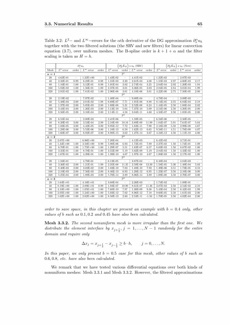
3.3. Numerical Results 65
Table 3.2: L2− and L∞−errors for the αth derivative of the DG approximation ∂αxuhtogether with the two filtered solutions (the SRV and new filters) for linear convectionequation (3.7), over uniform meshes. The B-spline order is k + 1 + α and the filterscaling is taken as H = h.
∂αx uh
(∂αHKH
)? uh (SRV)
(∂αHKH
)? uh (New)
Mesh L2 error order L∞ error order L2 error order L∞ error order L2 error order L∞ error order
α = 1 P1
20 4.62E-01 – 1.22E+00 – 1.43E-02 – 4.41E-02 – 1.22E-02 – 2.07E-02 –40 2.32E-01 0.99 6.22E-01 0.98 1.55E-03 3.20 2.61E-03 4.08 1.55E-03 2.97 4.60E-03 2.1780 1.16E-01 1.00 3.12E-01 0.99 1.91E-04 3.02 2.74E-04 3.25 2.04E-04 2.92 1.20E-03 1.94160 5.82E-02 1.00 1.56E-01 1.00 2.37E-05 3.01 3.36E-05 3.03 2.84E-05 2.84 3.01E-04 1.99320 2.91E-02 1.00 7.81E-02 1.00 2.96E-06 3.01 4.18E-06 3.01 4.22E-06 2.75 7.50E-05 2.00
P2
20 2.19E-02 – 7.97E-02 – 1.40E-04 – 9.00E-04 – 4.78E-04 – 3.09E-03 –40 5.48E-03 2.00 2.01E-02 1.98 6.69E-07 7.71 1.91E-06 8.88 8.14E-05 2.55 6.83E-04 2.1880 1.37E-03 2.00 5.05E-03 2.00 1.69E-08 5.31 2.52E-08 6.24 1.44E-05 2.50 1.68E-04 2.02160 3.43E-04 2.00 1.26E-03 2.00 5.13E-10 5.04 7.37E-10 5.09 2.54E-06 2.50 4.20E-05 2.00320 8.56E-05 2.00 3.16E-04 2.00 2.14E-11 4.58 3.04E-11 4.60 4.50E-07 2.50 1.05E-05 2.00
P3
20 6.55E-04 – 2.80E-03 – 2.41E-06 – 1.59E-05 – 6.24E-06 – 2.50E-05 –40 8.20E-05 3.00 3.53E-04 2.99 2.10E-09 10.16 3.89E-09 11.99 1.04E-07 5.91 7.61E-07 5.0480 1.02E-05 3.00 4.42E-05 3.00 9.95E-12 7.72 1.63E-11 7.90 2.18E-09 5.58 2.99E-08 4.67160 1.28E-06 3.00 5.53E-06 3.00 1.10E-13 6.50 1.62E-13 6.65 9.58E-11 4.51 1.78E-09 4.07320 1.60E-07 3.00 6.92E-07 3.00 8.98E-15 3.62 1.27E-14 3.67 4.24E-12 4.50 1.11E-10 4.00
α = 2 P2
20 2.67E+00 – 6.96E+00 – 7.20E-04 – 4.12E-03 – 6.42E-02 – 3.71E-01 –40 1.34E+00 1.00 3.50E+00 0.99 5.90E-06 6.93 1.73E-05 7.89 2.27E-02 1.50 1.74E-01 1.0980 6.70E-01 1.00 1.75E+00 1.00 1.29E-07 5.51 1.83E-07 6.57 8.03E-03 1.50 8.67E-02 1.00160 3.35E-01 1.00 8.78E-01 1.00 3.55E-09 5.19 5.02E-09 5.19 2.84E-03 1.50 4.33E-02 1.00320 1.67E-01 1.00 4.39E-01 1.00 1.39E-10 4.67 1.97E-10 4.67 1.00E-03 1.50 2.17E-02 1.00
P3
20 1.34E-01 – 4.78E-01 – 6.13E-05 – 3.87E-04 – 6.48E-04 – 4.84E-03 –40 3.36E-02 2.00 1.21E-01 1.99 2.35E-08 11.35 3.59E-08 13.39 1.58E-05 5.36 1.49E-04 5.0380 8.40E-03 2.00 3.02E-02 2.00 1.03E-10 7.83 1.48E-10 7.93 1.39E-06 3.51 1.73E-05 3.10160 2.10E-03 2.00 7.56E-03 2.00 8.46E-13 6.93 1.20E-12 6.95 1.23E-07 3.50 2.16E-06 3.00320 5.25E-04 2.00 1.89E-03 2.00 5.70E-14 3.89 8.06E-14 3.89 1.09E-08 3.50 2.70E-07 3.00
α = 3 P3
20 1.64E+01 – 4.16E+01 – 3.68E-04 – 2.26E-03 – 1.74E-02 – 1.09E-01 –40 8.19E+00 1.00 2.09E+01 0.99 1.93E-07 10.90 8.61E-07 11.36 3.07E-03 2.50 2.54E-02 2.1080 4.10E+00 1.00 1.05E+01 1.00 7.68E-10 7.97 1.30E-09 9.38 5.43E-04 2.50 6.42E-03 1.99160 2.05E+00 1.00 5.24E+00 1.00 5.93E-12 7.02 8.96E-12 7.18 9.60E-05 2.50 1.61E-03 2.00320 1.02E+00 1.00 2.62E+00 1.00 8.50E-13 2.80 2.53E-11 -1.50 1.70E-05 2.50 4.02E-04 2.00
order to save space, in this chapter we present an example with b = 0.4 only, othervalues of b such as 0.1, 0.2 and 0.45 have also been calculated.
Mesh 3.3.2. The second nonuniform mesh is more irregular than the first one. Wedistribute the element interface by xj+ 1
2, j = 1, . . . , N − 1 randomly for the entire
domain and require only
∆xj = xj+ 12− xj− 1
2≥ b · h, j = 0, . . . , N.
In this paper, we only present b = 0.5 case for this mesh, other values of b such as0.6, 0.8, etc. have also been calculated.
We remark that we have tested various differential equations over both kinds ofnonuniform meshes: Mesh 3.3.1 and Mesh 3.3.2. However, the filtered approximations

66 Chapter 3. Derivative SIAC Filters
DG SRV Newα = 1
0.0 0.2 0.4 0.6 0.8 1.0x
10−12
10−8
10−4
100
|erro
r|
N = 20N = 40N = 80N = 160
0.0 0.2 0.4 0.6 0.8 1.0x
10−12
10−8
10−4
100
|erro
r|
N = 20N = 40N = 80N = 160
0.0 0.2 0.4 0.6 0.8 1.0x
10−12
10−8
10−4
100
|erro
r|
N = 20N = 40N = 80N = 160
α = 2
0.0 0.2 0.4 0.6 0.8 1.0x
10−12
10−8
10−4
100
|erro
r|
N = 20N = 40N = 80N = 160
0.0 0.2 0.4 0.6 0.8 1.0x
10−12
10−8
10−4
100|er
ror|
N = 20N = 40N = 80N = 160
0.0 0.2 0.4 0.6 0.8 1.0x
10−12
10−8
10−4
100
|erro
r|
N = 20N = 40N = 80N = 160
Figure 3.4: The point-wise errors in log scale of the first and second derivatives of theDG approximation ∂αxuh together with the two filtered solutions (the SRV and newfilters) for linear equation (3.7), over uniform meshes. The B-spline order is k+1+α,the filter scaling is taken as H = h, and k = 2.
have similar performance since the performance mainly depends on the mesh. In orderto save space, we present one equation for each nonuniform mesh.
Comparison of the SRV filter and new filter over Nonuniform Mesh 3.3.1
In Chapter 2, we showed that the SRV filter has worse performance compared to thenew position-dependent filter over nonuniform meshes for filtering the solution itself.We also mentioned that the enormous support size of the SRV filter causes problems:we have to rescale the SRV filter to fit the domain size then we can not guarantee eitherthe accuracy order nor error reduction. Table 3.1 shows the minimum requirementof the number of elements for the SRV filter, and we can see that it is difficult tosatisfy. Based on these deficiencies, we conclude that the SRV filter is not suitable forapproximating derivatives over nonuniform meshes. However, in order to provide acomplete view of the position-dependent derivative filters, we still give one example ofusing the SRV filter for the first derivative over Mesh 3.3.1. Table 3.4 shows that withthe SRV filter, the filtered solutions (no matter what order of B-splines are used) areeven worse than the derivative of the DG approximation. In the rest of this section,we focus on testing the new filter over nonuniform meshes.
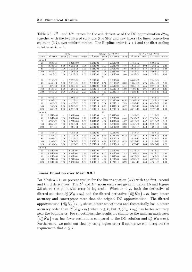
3.3. Numerical Results 67
Table 3.3: L2− and L∞−errors for the αth derivative of the DG approximation ∂αxuhtogether with the two filtered solutions (the SRV and new filters) for linear convectionequation (3.7), over uniform meshes. The B-spline order is k+ 1 and the filter scalingis taken as H = h.
∂αx uh ∂αx (KH ? uh) (SRV) ∂αx (KH ? uh) (New)Mesh L2 error order L∞ error order L2 error order L∞ error order L2 error order L∞ error order
α = 1 P1
20 4.62E-01 – 1.22E+00 – 1.25E-02 – 2.52E-02 – 1.45E-02 – 6.89E-02 –40 2.32E-01 0.99 6.22E-01 0.98 1.53E-03 3.03 2.25E-03 3.48 1.91E-03 2.92 1.28E-02 2.4380 1.16E-01 1.00 3.12E-01 0.99 1.91E-04 3.01 2.72E-04 3.05 2.63E-04 2.86 2.64E-03 2.28160 5.82E-02 1.00 1.56E-01 1.00 2.38E-05 3.00 3.38E-05 3.01 3.84E-05 2.78 5.90E-04 2.16320 2.91E-02 1.00 7.81E-02 1.00 2.96E-06 3.00 4.22E-06 3.00 5.95E-06 2.69 1.39E-04 2.09
P2
20 2.19E-02 – 7.97E-02 – 5.03E-05 – 3.23E-04 – 5.66E-05 – 2.84E-04 –40 5.48E-03 2.00 2.01E-02 1.98 5.38E-07 6.55 9.68E-07 8.38 1.05E-06 5.75 8.34E-06 5.0980 1.37E-03 2.00 5.05E-03 2.00 1.51E-08 5.16 2.22E-08 5.44 2.25E-08 5.55 2.87E-07 4.86160 3.43E-04 2.00 1.26E-03 2.00 4.83E-10 4.96 6.93E-10 5.00 7.49E-10 4.91 1.39E-08 4.37320 8.56E-05 2.00 3.16E-04 2.00 2.10E-11 4.53 2.98E-11 4.54 3.22E-11 4.54 8.03E-10 4.12
P3
20 6.55E-04 – 2.80E-03 – 9.62E-07 – 6.45E-06 – 4.03E-06 – 1.64E-05 –40 8.20E-05 3.00 3.53E-04 2.99 1.34E-09 9.48 2.51E-09 11.33 3.56E-08 6.83 2.59E-07 5.9880 1.02E-05 3.00 4.42E-05 3.00 6.65E-12 7.66 1.09E-11 7.85 4.55E-10 6.29 6.34E-09 5.35160 1.28E-06 3.00 5.53E-06 3.00 9.66E-14 6.11 1.41E-13 6.27 1.95E-11 4.55 3.50E-10 4.18320 1.60E-07 3.00 6.92E-07 3.00 8.92E-15 3.44 1.26E-14 3.48 8.61E-13 4.50 2.17E-11 4.01
α = 2 P2
20 2.67E+00 – 6.96E+00 – 1.94E-04 – 5.41E-04 – 1.14E-03 – 1.11E-02 –40 1.34E+00 1.00 3.50E+00 0.99 1.19E-05 4.03 2.50E-05 4.44 7.49E-05 3.92 7.18E-04 3.9580 6.70E-01 1.00 1.75E+00 1.00 7.42E-07 4.00 1.49E-06 4.07 6.31E-06 3.57 8.11E-05 3.15160 3.35E-01 1.00 8.78E-01 1.00 4.64E-08 4.00 9.73E-08 3.93 5.45E-07 3.53 9.89E-06 3.04320 1.67E-01 1.00 4.39E-01 1.00 2.90E-09 4.00 6.16E-09 3.98 4.76E-08 3.52 1.22E-06 3.02
P3
20 1.34E-01 – 4.78E-01 – 5.93E-06 – 4.03E-05 – 1.24E-04 – 1.02E-03 –40 3.36E-02 2.00 1.21E-01 1.99 1.04E-08 9.15 1.91E-08 11.05 2.22E-07 9.12 2.66E-06 8.5880 8.40E-03 2.00 3.02E-02 2.00 5.43E-11 7.58 1.20E-10 7.31 3.92E-10 9.15 7.91E-09 8.39160 2.10E-03 2.00 7.56E-03 2.00 7.45E-13 6.19 1.70E-12 6.15 5.52E-12 6.15 1.03E-10 6.27320 5.25E-04 2.00 1.89E-03 2.00 5.65E-14 3.72 9.20E-14 4.21 1.67E-13 5.05 5.58E-12 4.20
α = 3 P3
20 1.64E+01 – 4.16E+01 – 3.87E-05 – 2.55E-04 – 4.23E-04 – 3.61E-03 –40 8.19E+00 1.00 2.09E+01 0.99 4.36E-07 6.47 1.12E-06 7.83 4.26E-06 6.63 5.85E-05 5.9580 4.10E+00 1.00 1.05E+01 1.00 1.48E-08 4.88 3.47E-08 5.01 8.67E-08 5.62 1.26E-06 5.54160 2.05E+00 1.00 5.24E+00 1.00 4.68E-10 4.98 1.09E-09 5.00 3.73E-09 4.54 6.67E-08 4.24320 1.02E+00 1.00 2.62E+00 1.00 1.48E-11 4.98 7.85E-11 3.79 1.65E-10 4.50 4.15E-09 4.01
Linear Equation over Mesh 3.3.1
For Mesh 3.3.1, we present results for the linear equation (3.7) with the first, secondand third derivatives. The L2 and L∞ norm errors are given in Table 3.5 and Figure3.6 shows the point-wise error in log scale. When α ≤ k, both the derivative of
filtered solutions ∂αx (KH ? uh) and the filtered derivative(∂αHKH
)? uh have better
accuracy and convergence rates than the original DG approximation. The filtered
approximation(∂αHKH
)? uh shows better smoothness and theoretically has a better
accuracy order than ∂αx (KH ? uh) when α ≤ k, but ∂αx (KH ? uh) has better accuracynear the boundaries. For smoothness, the results are similar to the uniform mesh case;(∂αHKH
)? uh has fewer oscillations compared to the DG solution and ∂αx (KH ? uh).
Furthermore, we point out that by using higher-order B-splines we can disregard therequirement that α ≤ k.

68 Chapter 3. Derivative SIAC Filters
DG SRV Newα = 1
0.0 0.2 0.4 0.6 0.8 1.0x
10−12
10−8
10−4
100
|erro
r|
N = 20N = 40N = 80N = 160
0.0 0.2 0.4 0.6 0.8 1.0x
10−12
10−8
10−4
100
|erro
r|
N = 20N = 40N = 80N = 160
0.0 0.2 0.4 0.6 0.8 1.0x
10−12
10−8
10−4
100
|erro
r|
N = 20N = 40N = 80N = 160
α = 2
0.0 0.2 0.4 0.6 0.8 1.0x
10−12
10−8
10−4
100
|erro
r|
N = 20N = 40N = 80N = 160
0.0 0.2 0.4 0.6 0.8 1.0x
10−12
10−8
10−4
100|er
ror|
N = 20N = 40N = 80N = 160
0.0 0.2 0.4 0.6 0.8 1.0x
10−12
10−8
10−4
100
|erro
r|
N = 20N = 40N = 80N = 160
Figure 3.5: The point-wise errors in log scale of the first and second derivatives of theDG approximation ∂αxuh together with the two filtered solutions (the SRV and newfilters) for linear equation (3.7), over uniform meshes. The B-spline order is k+1, thefilter scaling is taken as H = h, and k = 2.
The point-wise error plots are given in Figure 3.6, the middle column is the fil-
tered approximation ∂αx (KH ? uh), which shows more oscillations than(∂αHKH
)? uh,
especially in the interior regions. We note, however that the support size of the filterthat uses a higher-order B-spline increases with the derivative order α and it slightlyincreases the computational cost. Near the boundaries, the filtered solutions have alarger error magnitude than those in the interior region. This is because near theboundaries we cannot use symmetric information around the filtered points, and thegeneral B-spline has less regularity compared to the central B-spline. We note that thecoarse meshes (such as N = 20 or even N = 40) are not sufficient to use the position-dependent derivative filter, the filtered solution may have larger errors compared tothe original DG approximation.
Variable Coefficient Equation over Mesh 3.3.2
After testing the constant coefficient equation (3.7), we move to a variable coefficientequation,
ut + (au)x = f, (x, t) ∈ [0, 1]× (0, T ]
u(x, 0) = sin(2πx),(3.8)

3.3. Numerical Results 69
Table 3.4: L2− and L∞−errors for the first derivative of the DG approximation ∂αxuh
together with the two filtered solution ∂αx (KH ? uh) and(∂αHKH
)? uh (with the SRV
filter) for linear equation (3.7), over Mesh 3.3.1. The filter scaling is taken as H = h2/5
near boundaries and H = h2/3 for the interior region (where the symmetric filter isapplied) .
∂αx uh ∂αx (KH ? uh)(∂αHKH
)? uh
Mesh L2 error order L∞ error order L2 error order L∞ error order L2 error order L∞ error order
P1
20 5.48E-01 – 1.76E+00 – 2.85E-01 – 1.49E+00 – 5.91E-01 – 2.54E+00 –40 2.82E-01 0.96 1.05E+00 0.74 2.63E-01 0.11 1.57E+00 -0.08 4.90E-01 0.27 2.37E+00 0.1080 1.37E-01 1.05 4.98E-01 1.08 2.11E-01 0.32 1.52E+00 0.05 4.17E-01 0.24 2.38E+00 -0.00160 6.72E-02 1.02 2.57E-01 0.96 1.29E-01 0.71 1.18E+00 0.36 3.08E-01 0.43 2.30E+00 0.05320 3.38E-02 0.99 1.30E-01 0.98 3.12E-02 2.05 3.75E-01 1.65 9.55E-02 1.69 9.77E-01 1.24
P2
20 3.56E-02 – 2.01E-01 – 1.15E-02 – 8.74E-02 – 3.30E-02 – 1.35E-01 –40 8.96E-03 1.99 5.80E-02 1.79 2.32E-03 2.31 1.90E-02 2.20 4.21E-03 2.97 2.41E-02 2.4980 1.96E-03 2.20 1.16E-02 2.32 2.08E-03 0.16 1.49E-02 0.35 3.70E-03 0.19 2.34E-02 0.05160 4.86E-04 2.01 3.88E-03 1.58 1.68E-03 0.30 1.49E-02 -0.00 3.16E-03 0.23 2.35E-02 -0.01320 1.32E-04 1.88 8.95E-04 2.11 1.36E-03 0.30 1.50E-02 -0.01 2.63E-03 0.27 2.36E-02 -0.01
P3
20 1.53E-03 – 1.10E-02 – 1.33E-02 – 7.20E-02 – 4.03E-02 – 2.58E-01 –40 2.10E-04 2.86 1.72E-03 2.68 7.05E-05 7.56 3.40E-04 7.73 4.44E-05 9.83 3.07E-04 9.7280 2.27E-05 3.21 1.80E-04 3.26 4.84E-06 3.86 3.58E-05 3.25 6.48E-06 2.78 4.29E-05 2.84160 2.72E-06 3.06 2.52E-05 2.84 3.30E-06 0.55 2.89E-05 0.31 5.84E-06 0.15 4.53E-05 -0.08320 3.42E-07 2.99 3.22E-06 2.97 2.71E-06 0.28 2.91E-05 -0.01 4.97E-06 0.23 4.55E-05 -0.01
where the variable coefficient is a(x, t) = 2+sin(2π(x+t)) and the forcing term, f(x, t),is chosen to make the exact solution
u(x, t) = sin(2π(x− t)).
As with the linear example, we present the L2 and L∞ errors in Table 3.6 with the firstthree derivatives over Mesh 3.3.2. The respective point-wise error plots (k = 2 case) areshown in Figure 3.7. The results are similar to the results for the constant coefficientcase. In order to save space we no longer repeat the descriptions, which are similar.However, we still want to point out one phenomenon. In this variable coefficient case,the filtered solution ∂αx (KH ? uh) shows somewhat better accuracy than the filtered
solution(∂αHKH
)? uh near the boundaries when α ≤ k. This performance suggests
that when α ≤ k we can consider not increasing the order of the B-splines, althoughit causes more oscillations in the error.
Remark 3.3.3. Here we conclude by discussing the consequences of using B-splinesof order k + 1 compared to using the usual order k + 1 + α; they are the following:
• it can give better accuracy near the boundaries;
• it can give better accuracy in the interior regions (when α k), but it damagesthe smoothness of filtered solution (more oscillations);
• it has a smaller support size;
• it allows the use of the symmetric filter over a larger area; and

70 Chapter 3. Derivative SIAC Filters
∂αxuh ∂αx (KH ? uh)(∂αHKH
)? uh
α = 1
0.0 0.2 0.4 0.6 0.8 1.0x
10−8
10−4
100
|erro
r|
N = 20N = 40N = 80N = 160
0.0 0.2 0.4 0.6 0.8 1.0x
10−8
10−4
100
|erro
r|
N = 20N = 40N = 80N = 160
0.0 0.2 0.4 0.6 0.8 1.0x
10−8
10−4
100
|erro
r|
N = 20N = 40N = 80N = 160
α = 2
0.0 0.2 0.4 0.6 0.8 1.0x
10−8
10−4
100
|erro
r|
N = 20N = 40N = 80N = 160
0.0 0.2 0.4 0.6 0.8 1.0x
10−8
10−4
100
|erro
r|
N = 20N = 40N = 80N = 160
0.0 0.2 0.4 0.6 0.8 1.0x
10−8
10−4
100
|erro
r|
N = 20N = 40N = 80N = 160
Figure 3.6: The point-wise errors in log scale for the first and second derivativesof DG approximation ∂αxuh together with the two filtered solutions ∂αx (KH ? uh) and(∂αHKH
)?uh (with the new filter) for linear convection equation (3.7) over Mesh 3.3.1.
The filter scaling is taken as H = h2/3, and k = 2.
• it requires α ≤ k.
Remark 3.3.4. We notice that in Tables 3.5 and 3.6, the accuracy order is smallerthan the conclusion in Theorem ??. The reason is twofold:
• The first one is the effect of the boundary region. The error magnitude of thefiltered solution in the interior region is much better than the error magnitude inthe boundary region. Therefore, the accuracy order in the L2 norm appears to beunstable and the numbers are smaller than the theoretical expectation. If we lookat Figures 3.6 and 3.7 (right column), the convergence rates are stable respectiveto boundary and interior regions separately.
• The second reason is that the Meshes 3.3.1 and 3.3.2 are randomly generated.There is no strict refined relation among the meshes. Therefore, the accuracyorder is affected by the randomness of the meshes, and a very stable accuracyorder is not observed. One can see that once the effect caused by randomnessbecomes smaller in the two-dimensional example, the accuracy order becomesstable, see Tables 3.7 and 3.8.

3.4. Two-Dimensional Example 71
∂αxuh ∂αx (KH ? uh)(∂αHKH
)? uh
α = 1
0.0 0.2 0.4 0.6 0.8 1.0x
10−8
10−4
100|er
ror|
N = 20N = 40N = 80N = 160
0.0 0.2 0.4 0.6 0.8 1.0x
10−8
10−4
100
|erro
r|
N = 20N = 40N = 80N = 160
0.0 0.2 0.4 0.6 0.8 1.0x
10−8
10−4
100
|erro
r|
N = 20N = 40N = 80N = 160
α = 2
0.0 0.2 0.4 0.6 0.8 1.0x
10−8
10−4
100
|erro
r|
N = 20N = 40N = 80N = 160
0.0 0.2 0.4 0.6 0.8 1.0x
10−8
10−4
100
|erro
r|
N = 20N = 40N = 80N = 160
0.0 0.2 0.4 0.6 0.8 1.0x
10−8
10−4
100
|erro
r|
N = 20N = 40N = 80N = 160
Figure 3.7: The point-wise errors in log scale of the first and second derivative ofthe DG approximation ∂αxuh together with the two filtered solutions ∂αx (KH ? uh) and(∂αHKH
)? uh (with the new filter) for variable coefficient equation (3.8) over Mesh
3.3.2. The filter scaling is taken as H = h2/3, and k = 2.
3.4 Two-Dimensional Example
For the two-dimensional example, we consider a 2D version of the linear hyperbolicequation
ut + ux + uy = 0, (x, y) ∈ [0, 1]× [0, 1],
u(x, y, 0) = sin(2πx+ 2πy),(3.9)
at time T = 1. The nonuniform meshes we used are the 2D quadrilateral extension ofMeshes 3.3.1 and 3.3.2. Here, we show the cross-derivative ∂2xy, the first derivatives ∂xand ∂y are omitted as they are similar to the 1D results. We give the L2 and L∞ errorin Tables 3.7 - 3.8 and the point-wise error plots in Figures 3.8 - 3.9. We note that thefiltered accuracy error seems slightly worse than the DG approximation over coarsemeshes, because near the boundary regions we need sufficiently refined meshes to showthe advantage of the position-dependent filter. Once the mesh is sufficient refined, wesee better results. We also note that although we require a relatively refined mesh forboundary regions, the results in the interior regions are always much better (see thepoint-wise error plots Figures 3.8 and 3.9).

72 Chapter 3. Derivative SIAC Filters
∂2xyuh ∂2xy(KH ? uh)(∂Hx∂HyKH
)? uh
Figure 3.8: The point-wise errors in log scale of the cross-derivative DG approximation∂2xyuh together with the filtered solution ∂2xyu
?h for the two-dimensional linear equation
(3.9) over Mesh 3.3.1 (2D, N = 160× 160).
∂2xyuh ∂2xy(KH ? uh)(∂Hx∂HyKH
)? uh
Figure 3.9: The point-wise errors in log scale of the cross-derivative DG approximation∂2xyuh together with the filtered solution ∂2xyu
?h for the two-dimensional linear equation
(3.9) over Mesh 3.3.1 (2D, N = 160× 160).
3.5 Conclusion
In this chapter, we have proposed three position-dependent derivative filter, to approx-imate the derivatives of a discontinuous Galerkin solution over uniform and nonuniformmeshes. These position-dependent derivative filters allow us to obtain more accuratederivatives of the DG solutions compared to calculating the derivatives of DG solu-tions directly. The derivative SRV filter uses 4k + 1 central B-splines, and obtains aconvergence rate of 2k+1 over uniform meshes regardless of derivative order. The newposition-dependent derivative filter uses 2k + 1 central B-splines and an extra generalB-spline, where the B-splines rely on the derivative order α. We have proved that thenew position-dependent derivative filter has accuracy order of µ(2k + 2) when usingfilter scaling H = hµ (µ ≈ 2/3). Additionally, we are able, for the first time, to extendthe symmetric derivative filter to nonuniform meshes. Through numerical examples,we compared the derivative SRV and new filter over uniform and nonuniform meshes.
3.5. Conclusion 73
We demonstrated that once the required conditions are satisfied the derivative SRVfilter has a better performance over uniform meshes compared to the new derivativefilter. However, for nonuniform meshes, only the new derivative filter can maintain itsperformance and improve the accuracy of the DG approximations. Also, we comparedderivative filters with different orders of B-splines: order k + 1 and order k + 1 + α.Numerical results indicate that using B-splines of order k+1 may improve the accuracyof the filtered solution near the boundaries. For interior regions where the symmetricderivative filtering is applied, using B-splines of order k+1+α shows better accuracyand smoothness. Lastly, we point out that for given nonuniform meshes there mayexist a better scaling that allows us to obtain better results.
Our new contributions are:
• Testing the position-dependent derivative filters for uniform meshes, which wasnot previously accomplished before;
• Applying the symmetric and position-dependent derivative filters over differentnonuniform meshes.
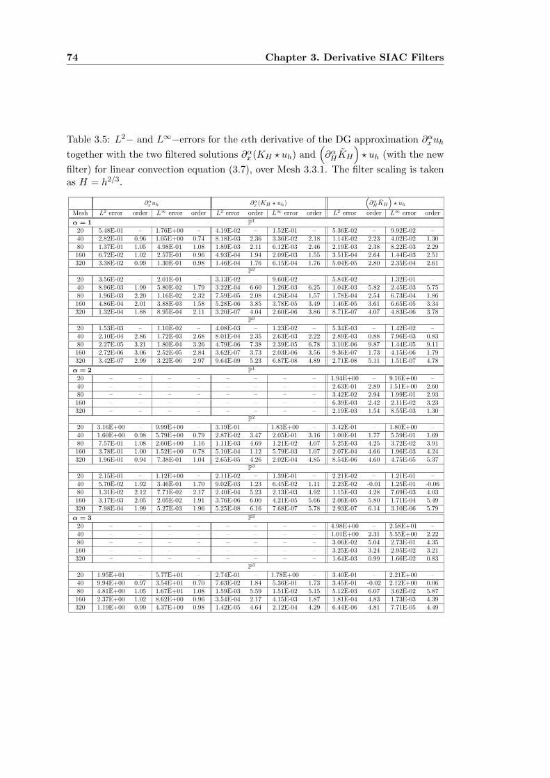
74 Chapter 3. Derivative SIAC Filters
Table 3.5: L2− and L∞−errors for the αth derivative of the DG approximation ∂αxuh
together with the two filtered solutions ∂αx (KH ? uh) and(∂αHKH
)? uh (with the new
filter) for linear convection equation (3.7), over Mesh 3.3.1. The filter scaling is takenas H = h2/3.
∂αx uh ∂αx (KH ? uh)(∂αHKH
)? uh
Mesh L2 error order L∞ error order L2 error order L∞ error order L2 error order L∞ error order
α = 1 P1
20 5.48E-01 – 1.76E+00 – 4.19E-02 – 1.52E-01 – 5.36E-02 – 9.92E-02 –40 2.82E-01 0.96 1.05E+00 0.74 8.18E-03 2.36 3.36E-02 2.18 1.14E-02 2.23 4.02E-02 1.3080 1.37E-01 1.05 4.98E-01 1.08 1.89E-03 2.11 6.12E-03 2.46 2.19E-03 2.38 8.22E-03 2.29160 6.72E-02 1.02 2.57E-01 0.96 4.93E-04 1.94 2.09E-03 1.55 3.51E-04 2.64 1.44E-03 2.51320 3.38E-02 0.99 1.30E-01 0.98 1.46E-04 1.76 6.15E-04 1.76 5.04E-05 2.80 2.35E-04 2.61
P2
20 3.56E-02 – 2.01E-01 – 3.13E-02 – 9.60E-02 – 5.84E-02 – 1.32E-01 –40 8.96E-03 1.99 5.80E-02 1.79 3.22E-04 6.60 1.26E-03 6.25 1.04E-03 5.82 2.45E-03 5.7580 1.96E-03 2.20 1.16E-02 2.32 7.59E-05 2.08 4.26E-04 1.57 1.78E-04 2.54 6.73E-04 1.86160 4.86E-04 2.01 3.88E-03 1.58 5.28E-06 3.85 3.78E-05 3.49 1.46E-05 3.61 6.65E-05 3.34320 1.32E-04 1.88 8.95E-04 2.11 3.20E-07 4.04 2.60E-06 3.86 8.71E-07 4.07 4.83E-06 3.78
P3
20 1.53E-03 – 1.10E-02 – 4.08E-03 – 1.23E-02 – 5.34E-03 – 1.42E-02 –40 2.10E-04 2.86 1.72E-03 2.68 8.01E-04 2.35 2.63E-03 2.22 2.89E-03 0.88 7.96E-03 0.8380 2.27E-05 3.21 1.80E-04 3.26 4.79E-06 7.38 2.39E-05 6.78 3.10E-06 9.87 1.44E-05 9.11160 2.72E-06 3.06 2.52E-05 2.84 3.62E-07 3.73 2.03E-06 3.56 9.36E-07 1.73 4.15E-06 1.79320 3.42E-07 2.99 3.22E-06 2.97 9.64E-09 5.23 6.87E-08 4.89 2.71E-08 5.11 1.51E-07 4.78
α = 2 P1
20 – – – – – – – – 1.94E+00 – 9.16E+00 –40 – – – – – – – – 2.63E-01 2.89 1.51E+00 2.6080 – – – – – – – – 3.42E-02 2.94 1.99E-01 2.93160 – – – – – – – – 6.39E-03 2.42 2.11E-02 3.23320 – – – – – – – – 2.19E-03 1.54 8.55E-03 1.30
P2
20 3.16E+00 – 9.99E+00 – 3.19E-01 – 1.83E+00 – 3.42E-01 – 1.80E+00 –40 1.60E+00 0.98 5.79E+00 0.79 2.87E-02 3.47 2.05E-01 3.16 1.00E-01 1.77 5.59E-01 1.6980 7.57E-01 1.08 2.60E+00 1.16 1.11E-03 4.69 1.21E-02 4.07 5.25E-03 4.25 3.72E-02 3.91160 3.78E-01 1.00 1.52E+00 0.78 5.10E-04 1.12 5.79E-03 1.07 2.07E-04 4.66 1.96E-03 4.24320 1.96E-01 0.94 7.38E-01 1.04 2.65E-05 4.26 2.02E-04 4.85 8.54E-06 4.60 4.75E-05 5.37
P3
20 2.15E-01 – 1.12E+00 – 2.11E-02 – 1.39E-01 – 2.21E-02 – 1.21E-01 –40 5.70E-02 1.92 3.46E-01 1.70 9.02E-03 1.23 6.45E-02 1.11 2.23E-02 -0.01 1.25E-01 -0.0680 1.31E-02 2.12 7.71E-02 2.17 2.40E-04 5.23 2.13E-03 4.92 1.15E-03 4.28 7.69E-03 4.03160 3.17E-03 2.05 2.05E-02 1.91 3.76E-06 6.00 4.21E-05 5.66 2.06E-05 5.80 1.71E-04 5.49320 7.98E-04 1.99 5.27E-03 1.96 5.25E-08 6.16 7.68E-07 5.78 2.93E-07 6.14 3.10E-06 5.79
α = 3 P2
20 – – – – – – – – 4.98E+00 – 2.58E+01 –40 – – – – – – – – 1.01E+00 2.31 5.55E+00 2.2280 – – – – – – – – 3.06E-02 5.04 2.73E-01 4.35160 – – – – – – – – 3.25E-03 3.24 2.95E-02 3.21320 – – – – – – – – 1.64E-03 0.99 1.66E-02 0.83
P3
20 1.95E+01 – 5.77E+01 – 2.74E-01 – 1.78E+00 – 3.40E-01 – 2.21E+00 –40 9.94E+00 0.97 3.54E+01 0.70 7.63E-02 1.84 5.36E-01 1.73 3.45E-01 -0.02 2.12E+00 0.0680 4.81E+00 1.05 1.67E+01 1.08 1.59E-03 5.59 1.51E-02 5.15 5.12E-03 6.07 3.62E-02 5.87160 2.37E+00 1.02 8.62E+00 0.96 3.54E-04 2.17 4.15E-03 1.87 1.81E-04 4.83 1.73E-03 4.39320 1.19E+00 0.99 4.37E+00 0.98 1.42E-05 4.64 2.12E-04 4.29 6.44E-06 4.81 7.71E-05 4.49

3.5. Conclusion 75
Table 3.6: L2− and L∞−errors for the αth derivative of the DG approximation ∂αxuh
together with the two filtered solutions ∂αx (KH ? uh) and(∂αHKH
)? uh (with the new
filter) for variable coefficient equation (3.8), over Mesh 3.3.2. The filter scaling is takenas H = h2/3.
∂αx uh ∂αx (KH ? uh)(∂αHKH
)? uh
Mesh L2 error order L∞ error order L2 error order L∞ error order L2 error order L∞ error order
α = 1 P1
20 5.73E-01 – 2.04E+00 – 4.28E-02 – 9.17E-02 – 4.04E-02 – 8.51E-02 –40 2.76E-01 1.05 9.98E-01 1.03 1.29E-02 1.73 6.62E-02 0.47 1.47E-02 1.46 5.53E-02 0.6280 1.53E-01 0.85 6.35E-01 0.65 3.44E-03 1.91 1.31E-02 2.34 2.72E-03 2.43 7.98E-03 2.79160 7.16E-02 1.10 3.43E-01 0.89 1.01E-03 1.76 5.63E-03 1.22 6.26E-04 2.12 1.82E-03 2.13320 4.07E-02 0.82 2.46E-01 0.48 9.81E-04 0.05 8.33E-03 -0.57 6.37E-04 -0.02 3.11E-03 -0.77
P2
20 6.60E-02 – 4.27E-01 – 3.38E-02 – 1.10E-01 – 6.16E-02 – 1.42E-01 –40 1.27E-02 2.38 9.22E-02 2.21 3.17E-04 6.73 1.26E-03 6.45 9.68E-04 5.99 2.46E-03 5.8580 2.12E-03 2.58 1.27E-02 2.87 7.71E-05 2.04 4.28E-04 1.55 1.78E-04 2.44 6.61E-04 1.89160 6.40E-04 1.73 5.66E-03 1.16 5.33E-06 3.85 3.71E-05 3.53 1.47E-05 3.60 6.54E-05 3.34320 2.48E-04 1.37 2.99E-03 0.92 4.67E-07 3.51 2.70E-06 3.78 8.72E-07 4.08 4.93E-06 3.73
P3
20 2.95E-03 – 2.29E-02 – 4.28E-03 – 1.29E-02 – 5.72E-03 – 1.52E-02 –40 2.88E-04 3.35 2.84E-03 3.01 8.01E-04 2.42 2.61E-03 2.31 2.89E-03 0.98 7.97E-03 0.9380 3.95E-05 2.87 3.84E-04 2.89 4.82E-06 7.38 2.36E-05 6.79 3.10E-06 9.87 1.41E-05 9.15160 4.74E-06 3.06 6.15E-05 2.64 3.62E-07 3.73 2.05E-06 3.53 9.36E-07 1.73 4.15E-06 1.76320 1.28E-06 1.89 2.14E-05 1.52 9.64E-09 5.23 6.95E-08 4.88 2.71E-08 5.11 1.51E-07 4.78
α = 2 P1
20 – – – – – – – – 2.45E+00 – 1.14E+01 –40 – – – – – – – – 4.39E-01 2.48 2.61E+00 2.1280 – – – – – – – – 6.57E-02 2.74 2.23E-01 3.55160 – – – – – – – – 3.48E-02 0.92 1.13E-01 0.98320 – – – – – – – – 5.99E-02 -0.78 2.80E-01 -1.31
P2
20 3.89E+00 – 1.40E+01 – 3.34E-01 – 2.36E+00 – 3.39E-01 – 2.26E+00 –40 1.78E+00 1.13 6.49E+00 1.10 2.93E-02 3.51 2.23E-01 3.40 1.03E-01 1.72 5.84E-01 1.9580 7.66E-01 1.22 2.54E+00 1.35 1.11E-03 4.72 9.19E-03 4.60 5.31E-03 4.28 3.73E-02 3.97160 4.10E-01 0.90 1.86E+00 0.45 2.28E-04 2.28 1.26E-03 2.87 1.86E-04 4.84 1.62E-03 4.52320 2.28E-01 0.85 1.36E+00 0.45 2.00E-04 0.19 1.38E-03 -0.14 1.39E-05 3.74 8.73E-05 4.22
P3
20 2.89E-01 – 1.67E+00 – 2.16E-02 – 1.63E-01 – 1.84E-02 – 1.13E-01 –40 6.24E-02 2.21 4.20E-01 1.99 9.03E-03 1.26 6.49E-02 1.33 2.22E-02 -0.28 1.25E-01 -0.1580 1.80E-02 1.79 1.27E-01 1.72 2.35E-04 5.27 2.09E-03 4.96 1.15E-03 4.28 7.60E-03 4.04160 4.12E-03 2.13 3.67E-02 1.79 3.66E-06 6.00 4.28E-05 5.61 2.06E-05 5.80 1.73E-04 5.46320 1.51E-03 1.45 1.79E-02 1.03 1.06E-07 5.10 7.61E-07 5.81 2.93E-07 6.14 3.11E-06 5.80
α = 3 P2
20 – – – – – – – – 6.75E+00 – 4.36E+01 –40 – – – – – – – – 1.18E+00 2.51 7.23E+00 2.5980 – – – – – – – – 2.36E-02 5.65 2.19E-01 5.04160 – – – – – – – – 7.55E-03 1.64 7.38E-02 1.57320 – – – – – – – – 1.28E-03 2.57 7.79E-03 3.24
P3
20 2.04E+01 – 6.86E+01 – 1.68E+00 – 1.10E+01 – 2.37E+00 – 1.56E+01 –40 9.76E+00 1.06 3.31E+01 1.05 9.36E-02 4.17 6.06E-01 4.18 3.52E-01 2.75 2.16E+00 2.8580 5.39E+00 0.86 2.14E+01 0.63 4.87E-04 7.59 3.77E-03 7.33 5.15E-03 6.10 3.73E-02 5.86160 2.52E+00 1.10 1.15E+01 0.89 1.55E-04 1.65 1.84E-03 1.04 1.76E-04 4.87 1.73E-03 4.43320 1.39E+00 0.86 7.30E+00 0.66 6.97E-05 1.16 5.24E-04 1.81 6.60E-06 4.74 7.91E-05 4.45

76 Chapter 3. Derivative SIAC Filters
Table 3.7: L2− and L∞−errors for the cross-derivative DG approximation ∂2xyuhtogether with the filtered solution ∂2xyu
?h for the two-dimensional linear equation (3.9)
over Mesh 3.3.1 (2D).
∂2xyuh ∂2xy(KH ? uh) ∂Hx∂Hy
KH ? uhMesh L2 error order L∞ error order L2 error order L∞ error order L2 error order L∞ error order
P1
20× 20 5.47E+00 – 2.32E+01 – – – – – 1.32E+00 – 1.25E+01 –40× 40 2.71E+00 1.01 1.33E+01 0.81 – – – – 1.97E-01 2.75 1.80E+00 2.7980× 80 1.33E+00 1.03 6.39E+00 1.06 – – – – 2.81E-02 2.81 2.56E-01 2.81
160× 160 6.62E-01 1.00 3.38E+00 0.92 – – – – 4.08E-03 2.78 3.39E-02 2.92P2
20× 20 3.48E-01 – 2.49E+00 – 4.68E-01 – 3.44E+00 – 5.66E-01 – 3.59E+00 –40× 40 8.16E-02 2.09 7.13E-01 1.80 2.65E-02 4.14 3.63E-01 3.24 5.38E-02 3.40 6.81E-01 2.4080× 80 1.93E-02 2.08 1.81E-01 1.98 1.38E-03 4.26 1.96E-02 4.22 2.83E-03 4.25 4.03E-02 4.08
160× 160 4.79E-03 2.01 4.53E-02 2.00 6.86E-05 4.33 8.74E-04 4.48 1.44E-04 4.30 1.84E-03 4.45P3
20× 20 1.54E-02 – 1.47E-01 – 4.11E-02 – 2.79E-01 – 4.06E-02 – 2.63E-01 –40× 40 1.75E-03 3.13 2.29E-02 2.68 1.14E-02 1.85 1.27E-01 1.13 2.45E-02 0.73 2.04E-01 0.3780× 80 2.00E-04 3.13 2.51E-03 3.19 2.42E-04 5.56 4.26E-03 4.90 5.30E-04 5.53 8.51E-03 4.58
160× 160 2.47E-05 3.02 3.58E-04 2.81 4.91E-06 5.62 8.59E-05 5.63 1.08E-05 5.62 1.81E-04 5.56
Table 3.8: L2− and L∞−errors for the cross-derivative DG approximation ∂2xyuhtogether with the filtered solution ∂2xyu
?h for the two-dimensional linear equation (3.9)
over Mesh 3.3.2 (2D).
∂2xyuh ∂2xy(KH ? uh) ∂Hx∂Hy
KH ? uhMesh L2 error order L∞ error order L2 error order L∞ error order L2 error order L∞ error order
P1
20× 20 6.03E+00 – 2.94E+01 – – – – – 1.53E+00 – 1.27E+01 –40× 40 3.20E+00 0.91 1.95E+01 0.59 – – – – 2.72E-01 2.50 2.07E+00 2.6280× 80 1.61E+00 0.99 1.09E+01 0.84 – – – – 5.44E-02 2.32 4.01E-01 2.37
160× 160 7.39E-01 1.12 5.18E+00 1.07 – – – – 8.35E-03 2.70 1.37E-01 1.55P2
20× 20 5.60E-01 – 7.00E+00 – 4.73E-01 – 3.48E+00 – 5.68E-01 – 3.59E+00 –40× 40 1.68E-01 1.73 2.65E+00 1.40 2.67E-02 4.15 3.67E-01 3.24 5.34E-02 3.41 6.88E-01 2.3880× 80 3.85E-02 2.13 5.30E-01 2.32 1.36E-03 4.29 1.94E-02 4.24 2.98E-03 4.16 4.12E-02 4.06
160× 160 7.27E-03 2.41 1.03E-01 2.37 7.90E-05 4.11 1.05E-03 4.21 1.54E-04 4.27 1.89E-03 4.44P3
20× 20 4.02E-02 – 3.66E-01 – 4.12E-02 – 2.79E-01 – 4.05E-02 – 2.64E-01 –40× 40 7.60E-03 2.40 1.03E-01 1.83 1.14E-02 1.86 1.29E-01 1.12 2.45E-02 0.72 2.06E-01 0.3680× 80 7.71E-04 3.30 1.68E-02 2.61 2.42E-04 5.55 4.21E-03 4.93 5.30E-04 5.53 8.40E-03 4.62
160× 160 5.76E-05 3.74 1.31E-03 3.69 4.91E-06 5.62 8.65E-05 5.60 1.08E-05 5.62 1.82E-04 5.51

4SIAC Filters over Nonuniform Meshes
In practical applications, there are strong motivators for the adoption of unstruc-tured meshes for handling complex geometries and using adaptive mesh refinementtechniques. Based on this practical necessity, it is widely believed that discontinuousGalerkin methods, which provide high-order accuracy on unstructured meshes, willbecome one of the standard numerical methods for future generations. However, SIACfilters are still limited primarily to structured meshes. For general nonuniform meshes,the quality of the filtered solution is usually unsatisfactory. The ability to deal withnonuniform meshes is an obstacle to the further development of SIAC filters.
In this chapter, we focus on applying the SIAC filter for DG solutions over nonuni-form meshes. Specifically, this study focuses on the barrier to applying the SIAC filterto nonuniform meshes – the scaling. We establish a relation between the filtered solu-tions and the unstructuredness of nonuniform meshes. Further, we demonstrate thatthere exist an optimal accuracy of the filtered solution for a given nonuniform mesh,and it is possible to approximate the optimal accuracy by the method we propose. Byapplying the newly designed SIAC filter over nonuniform meshes, the filtered solutionhas demonstrated improvement in accuracy order as well as improve the quality ofthe numerical solution. The key concept in the extension to unstructured meshes isunderstanding the divided differences, as discussed in the following section.
4.1 Divided Differences: Uniform Meshes
In order to use the SIAC filter to improve the quality of DG solutions over nonuniformmeshes, we need to study the theoretical challenges of using the SIAC filter, namelythe divided differences of DG solutions. To get full appreciation of the situation, webegin discussing from the uniform meshes in this section.
As presented in Chapter 1, Theorem 1.2.1 is the theoretical foundation of usingSIAC filters for DG approximations. Theorem 1.2.1 shows that the divided differencesof the DG solution have the same accuracy order as the DG solution itself in the L2
norm (1.3) and the negative order norm (1.4). When the divided difference of orderα = 0, the conclusion is well known and studied. Nevertheless, the estimates for α > 0are equally important for the theoretical foundations of the SIAC filter. In [25], after
77
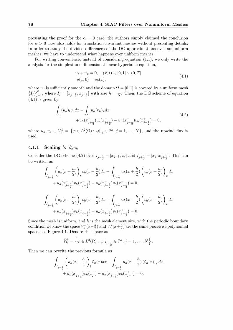
78 Chapter 4. SIAC Filters over Nonuniform Meshes
presenting the proof for the α = 0 case, the authors simply claimed the conclusionfor α > 0 case also holds for translation invariant meshes without presenting details.In order to study the divided differences of the DG approximations over nonuniformmeshes, we have to understand what happens over uniform meshes.
For writing convenience, instead of considering equation (1.1), we only write theanalysis for the simplest one-dimensional linear hyperbolic equation,
ut + ux = 0, (x, t) ∈ [0, 1]× (0, T ]
u(x, 0) = u0(x),(4.1)
where u0 is sufficiently smooth and the domain Ω = [0, 1] is covered by a uniform meshIjNj=1, where Ij = [xj− 1
2, xj+ 1
2] with size h = 1
N . Then, the DG scheme of equation
(4.1) is given by∫Ij
(uh)tvhdx−∫Ij
uh(vh)xdx
+uh(x−j+ 1
2
)vh(x−j+ 1
2
)− uh(x−j− 12
)vh(x+j− 1
2
) = 0,(4.2)
where uh, vh ∈ V kh =
ϕ ∈ L2(Ω) : ϕ|Ij ∈ Pk, j = 1, . . . , N
, and the upwind flux is
used.
4.1.1 Scaling h: ∂huh
Consider the DG scheme (4.2) over Ij− 12= [xj−1, xj ] and Ij+ 1
2= [xj , xj+ 1
2]. This can
be written as∫Ij− 1
2
(uh(x+
h
2)
)t
vh(x+h
2)dx−
∫Ij− 1
2
uh(x+h
2)
(vh(x+
h
2)
)x
dx
+ uh(x−j+ 1
2
)vh(x−j+ 1
2
)− uh(x−j− 12
)vh(x+j− 1
2
) = 0,
∫Ij+1
2
(uh(x−
h
2)
)t
vh(x−h
2)dx−
∫Ij+1
2
uh(x−h
2)
(vh(x−
h
2)
)x
dx
+ uh(x−j+ 1
2
)vh(x−j+ 1
2
)− uh(x−j− 12
)vh(x+j− 1
2
) = 0.
Since the mesh is uniform, and h is the mesh element size, with the periodic boundarycondition we know the space V k
h (x−h2 ) and V
kh (x+
h2 ) are the same piecewise polynomial
space, see Figure 4.1. Denote this space as
V kh =
ϕ ∈ L2(Ω) : ϕ|I
j− 12
∈ Pk, j = 1, . . . , N.
Then we can rewrite the previous formula as∫Ij− 1
2
(uh(x+
h
2)
)t
vh(x)dx−∫Ij− 1
2
uh(x+h
2) (vh(x))x dx
+ uh(x−j+ 1
2
)vh(x−j )− uh(x
−j− 1
2
)vh(x+j−1) = 0,
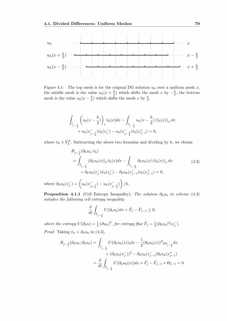
4.1. Divided Differences: Uniform Meshes 79
uh x
uh(x+ h2 ) x− h
2
uh(x− h2 ) x+ h
2
Figure 4.1: The top mesh is for the original DG solution uh over a uniform mesh x,the middle mesh is the value uh(x + h
2 ) which shifts the mesh x by −h2 , the bottom
mesh is the value uh(x− h2 ) which shifts the mesh x by h
2 .
∫Ij− 1
2
(uh(x−
h
2)
)t
vh(x)dx−∫Ij− 1
2
uh(x−h
2) (vh(x))x dx
+ uh(x−j− 1
2
)vh(x−j )− uh(x
−j− 3
2
)vh(x+j−1) = 0,
where vh ∈ V kh . Subtracting the above two formulas and dividing by h, we obtain
Bj− 12(∂huh; vh)
=
∫Ij− 1
2
(∂huh(x))t vh(x)dx−∫Ij− 1
2
∂huh(x) (vh(x))x dx
+ ∂huh(x−j )vh(x
−j )− ∂huh(x
−j−1)vh(x
+j−1) = 0,
(4.3)
where ∂huh(x−j ) =
(uh(x
−j+ 1
2
)− uh(x−j− 12
)
)/h.
Proposition 4.1.1 (Cell Entropy Inequality). The solution ∂huh to scheme (4.3)satisfies the following cell entropy inequality
d
dt
∫Ij− 1
2
U(∂huh)dx+ Fj − Fj−1 ≤ 0,
where the entropy U(∂hu) =12 (∂uh)
2, for entropy flux Fj =12(∂huh)
2(x−j ).
Proof. Taking vh = ∂huh in (4.3),
Bj− 12(∂huh; ∂huh) =
∫Ij− 1
2
U(∂huh(x))tdx−1
2(∂huh(x))
2|∂Ij− 1
2
dx
+ (∂huh(x−j ))
2 − ∂huh(x−j−1)∂huh(x+j−1)
=d
dt
∫Ij− 1
2
U(∂huh(x))dx+ Fj − Fj−1 +Θj−1 = 0

80 Chapter 4. SIAC Filters over Nonuniform Meshes
where
Θj−1 =1
2
(∂huh(x
+j−1)− ∂huh(x
−j−1)
)2≥ 0
This completes the proof of the cell entropy inequality.
Similar to the primary value uh, we also have
Proposition 4.1.2 (L2 stability). For periodic boundary conditions, the divided dif-ference, ∂huh, to scheme (4.3) satisfies the following L2 stability condition
d
dt
∫ 1
0(∂huh)
2 dx ≤ 0 or ‖∂huh(·, t)‖ ≤ ‖∂huh(·, 0)‖.
Proposition 4.1.3 (Error Estimate). The divided difference ∂huh of DG scheme (4.2)for equation (4.1) with a smooth solution u satisfies the following error estimates. Inthe L2 norm:
‖∂hu− ∂huh‖0,Ω ≤ Chk+1,
and in the negative order norm:
‖∂hu− ∂huh‖−(k+1),Ω ≤ Chk+1,
where C depends on u and its derivatives but is independent of h.
Remark 4.1.1. Using induction, the above propositions also hold for α > 1.
4.1.2 Constant Scaling H: ∂Huh
In the previous analysis, we give the error estimate of the divided difference of the DGsolution ∂huh with the scaling h, where h is the uniform mesh size. In this section,we investigate the behavior of using a general constant scaling H. Based on the DGscheme (4.2), similar to using scaling h, we have∫
Ij−H2
(uh(x+
H
2)
)t
vh(x+H
2)dx−
∫Ij−H
2
uh(x+H
2)
(vh(x+
H
2)
)x
dx
+ uh(x−j+ 1
2
)vh(x−j+ 1
2
)− uh(x−j− 12
)vh(x+j− 1
2
) = 0,
∫Ij+
H2
(uh(x−
H
2)
)t
vh(x−H
2)dx−
∫Ij+
H2
uh(x−H
2)
(vh(x−
H
2)
)x
dx
+ uh(x−j+ 1
2
)vh(x−j+ 1
2
)− uh(x−j− 12
)vh(x+j− 1
2
) = 0,
If H = h, then the situation will follow the previous analysis, we can subtract theabove two formulas directly. However, if H 6= h, then things become complicated. Wecan not subtract them directly like in the H = h case, since the space V k
h (x−H2 ) and
V kh (x+ H
2 ) are no longer the same space, see Figure 4.2. Once the spaces V kh (x−
H2 )
and V kh (x+
H2 ) are not the same space, the traditional analysis techniques can not be
performed. Therefore, in order to obtain a scheme for ∂Huh, we have to require the

4.1. Divided Differences: Uniform Meshes 81
uh x
uh(x+ H2 ) x− H
2
uh(x− H2 ) x+ H
2
Figure 4.2: The top mesh is the original DG solution uh over a uniform mesh x, themiddle mesh is the value uh(x + H
2 ) which means shifting the mesh x by −H2 , the
bottom mesh is the value uh(x− H2 ) which shifts the mesh x by H
2 .
scaling H to satisfy some other conditions. For uniform mesh with periodic conditions,we need a scaling H which makes the space V k
h (x −H2 ) and V k
h (x + H2 ) be the same
polynomial space. This requires
Ij −H
2+mh = Ij +
H
2,
where m is a positive integer. The above relation is equivalent to
H = mh.
Figure 4.3 shows a example with the scaling H = 2h.
uh x
uh(x+ H2 ) x− H
2
uh(x− H2 ) x+ H
2
H = 2h
Figure 4.3: The top mesh is the original DG solution uh over a uniform mesh x, themiddle mesh is the value uh(x + H
2 ) which means shifting the mesh x by −H2 , the
bottom mesh is the value uh(x− H2 ) which shifts the mesh x by H
2 . Here, H = 2h.
When H = mh, denote
V kh = V k
h (x+H
2) = V k
h (x−H
2),

82 Chapter 4. SIAC Filters over Nonuniform Meshes
we have ∫Ij−m
2
(uh(x+
mh
2)
)t
vh(x)dx−∫Ij−m
2
uh(x+mh
2) (vh(x))x dx
+ uh(x−j+ 1
2
)vh(x−j−m−1
2
)− uh(x−j− 12
)vh(x+j−1−m−1
2
) = 0,
∫Ij−m
2
(uh(x−
mh
2)
)t
vh(x)dx−∫Ij−m
2
uh(x−mh
2) (vh(x))x dx
+ uh(x−j−m+ 1
2
)vh(x−j−m−1
2
)− uh(x−j−m− 12
)vh(x+j−1−m−1
2
) = 0,
where vh ∈ V kh . Subtracting the above two formulas and dividing by H = mh, we
obtain ∫Ij−m
2
(∂Huh(x))t vh(x)dx−∫Ij−m
2
∂Huh(x) (vh(x))x dx
+ ∂Huh(x−j−m−1
2
)vh(x−j−m−1
2
)− ∂Huh(x−j−1−m−12
)vh(x+j−1−m−1
2
) = 0,
where ∂Huh(xj−m−12
) =
(uh(x
−j+ 1
2
)− uh(x−j−m+ 12
)
)/(mh). The rest of the analysis is
same as the ∂huh case. We then have the following corollaries:
Corollary 4.1.4. Under the same conditions as in Theorem 1.2.1. The divided dif-ferences of the DG approximation, ∂αHuh in the L2 norm have the error
‖∂αH(u− uh)‖0,Ω ≤ Chk+1,
and in the negative order norm:
‖∂αH(u− uh)‖−(k+1),Ω ≤ Ch2k+1,
where H = mh and α = (α1, . . . , αd) is an arbitrary multi-index.
Corollary 4.1.5. Under the same conditions as in Theorem 1.3.4, the scaling H =mh, then
‖u−K(2k+1,k+1)H ? uh‖0,Ω0 ≤ Ch2k+1.
Remark 4.1.2. Aside from H = mh case, it is very difficult to analyze the rest of thecases. Numerical examples suggest that the accuracy order is drops from 2k + 1 foruniform meshes.
Although it is very difficult to analyze a general scaling H directly, when H is veryclose to a known results such as h or mh we can take advantage of the known resultsto bound ∂αH(u− uh).

4.2. Divided Differences: Nonuniform Meshes 83
For example, considering a scaling of H = (1− c ·h)h or H = (1−O(h))h. Denotethe error e = u− uh. For the first divided difference of the DG error e, we have:
∂He =1
H
(e(x+
1
2h− c
2h2)− e(x− 1
2h+
c
2h2)
)=
1
H
(e(x+
1
h)− ch2
2e′(x+
1
h) +
1
2e(2)(ξ)
(ch2
2
)2)
−
(e(x− 1
h) +
ch2
2e′(x− 1
h) +
1
2e(2)(ζ)
(ch2
2
)2)
=1
(1− c · h)h
h∂he−
ch2
2
(e′(x+
1
h) + e′(x− 1
h)
)+O(h4)
=
1
(1− c · h)
∂he−
ch
2
(e′(x+
1
h) + e′(x− 1
h)
)+O(h3)
In the L2 norm, then
‖∂He‖0 ≤ C0‖∂he‖0 + C1h‖e′‖+ C2h3‖e(2)‖.
Since ‖e(i)‖0 ≤ C‖e‖i ≤ Ch−i‖e‖0 ≤ Chk+1−i , we have
‖∂He‖0 ≤ C0‖∂he‖0 + C3hk+1.
Now, we have shown that using a scaling H = (1 − c · h)h has no negative effect onthe accuracy order of the divided differences of the DG error. In fact, we can changethe value of c to approach the optimal accuracy for the filtered solution in the L2
norm (usually the optimal value of c is larger than zero and the respective scalingH = (1− c · h)h < h).
4.2 Divided Differences: Nonuniform Meshes
After investigation of the divided differences of DG solutions for uniform meshes, wemove to nonuniform meshes. Since we do not know what is the suitable scaling fornonuniform meshes, we use the scaling H to represent a general scaling.
Similar to using a general scaling H for uniform meshes, the challenge is to foruh(x + H
2 ) and uh(x − H2 ) to be in the a same space. Figure 4.4 indicates a general
situation of the first divided difference. We can see that the situation is much worse inFigure 4.4 than in Figure 4.2. For a general nonuniform mesh, it is almost impossibleto find a constant scaling H such that uh(x + H
2 ) and uh(x −H2 ) belong to the same
approximation space. In other words, for general nonuniform meshes, we can notprovide a traditional analysis such as the error estimates for uniform meshes.
Therefore, we have to find a different way of finding a suitable scaling for nonuni-form meshes. Generally speaking, there are two possible directions to consider:
• Using known results (results over uniform meshes or smoothly-varying meshes)to bound the errors over nonuniform meshes. This is the method we used toanalyze the results over smoothness-varying meshes in Chapter 2.

84 Chapter 4. SIAC Filters over Nonuniform Meshes
uh x
uh(x+ H2 ) x− H
2
uh(x− H2 ) x+ H
2
Figure 4.4: The top mesh is the original DG solution uh over a nonuniform mesh x,the middle mesh is the value uh(x+
H2 ) which means shifting the mesh x by −H
2 , thebottom mesh is the value uh(x− H
2 ) which shifts the mesh x by H2 .
• Considering a variable scaling H(x) to force the divided difference components,uh(x + H
2 ) and uh(x − H2 ), into the same space. Then, processing the same
analysis as used in Section 4.1.
4.2.1 Variable Scaling H(x)
In this section, we first consider the idea of using a variable scaling H(x), x ∈ Ω.For the first divided difference, we try to choose an H(x) such that uh(x + H
2 ) anduh(x− H
2 ) are in the same space. For element Ij = [xj− 12, xj+ 1
2], we denote that
Ij ±H
2=
x± H(x)
2, x ∈ Ij
,
of course, we require x± H(x)2 are monotonically increasing with x. In order to get the
same space we require that (the choice is the simplest one but not unique)
Ij +H
2= Ij+1 −
H
2, j = 1, . . . , N − 1.(the choice is not unique)
Denote H(xj−1/2) = Hj−1/2, this gives
xj−1/2 +Hj−1/2
2= xj+1/2 −
Hj+1/2
2j = 1, . . . , N − 1,
or,
1
2
(H1/2 +H3/2
)= ∆x1
1
2
(H3/2 +H5/2
)= ∆x2
. . .
1
2
(HN−1/2 +HN+1/2
)= ∆xN .
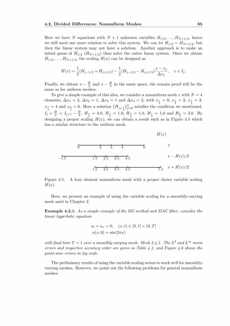
4.2. Divided Differences: Nonuniform Meshes 85
Here we have N equations with N + 1 unknown variables H1/2, . . . , HN+1/2, hencewe still need one more relation to solve this system. We can let H1/2 = HN+1/2, butthen the linear system may not have a solution. Another approach is to make aninitial guess of H1/2 (HN+1/2) then solve the entire linear system. Once we obtainH1/2, . . . , HN+1/2, the scaling H(x) can be designed as
H(x) =1
2(Hj−1/2 +Hj+1/2)−
1
2(Hj−1/2 −Hj+1/2)
x− xj∆xj
, x ∈ Ij .
Finally, we obtain x − H2 and x − H
2 in the same space, the remain proof will be thesame as for uniform meshes.
To give a simple example of this idea, we consider a nonuniform mesh x with N = 4elements, ∆x1 = 2, ∆x2 = 1, ∆x3 = 1 and ∆x4 = 2, with x 1
2= 0, x 3
2= 2, x 5
2= 3,
x 72= 4 and x 9
2= 6. Here a solution Hj+ 1
24j=0 satisfies the condition we mentioned,
Ij +H2 = Ij+1 − H
2 , H 12= 3.0, H 3
2= 1.0, H 5
2= 1.0, H 7
2= 1.0 and H 9
2= 3.0. By
designing a proper scaling H(x), we can obtain a result such as in Figure 4.5 whichhas a similar structure to the uniform mesh.
0 2 3 4 6x
−1.5 1.5 2.5 3.5 4.5x−H(x)/2
1.5 2.5 3.5 4.5 7.5x+H(x)/2
H(x)
Figure 4.5: A four element nonuniform mesh with a proper choice variable scalingH(x).
Here, we present an example of using the variable scaling for a smoothly-varyingmesh used in Chapter 2.
Example 4.2.1. As a simple example of the DG method and SIAC filter, consider thelinear hyperbolic equation
ut + ux = 0, (x, t) ∈ [0, 1]× (0, T ]
u(x, 0) = sin(2πx)
with final time T = 1 over a smoothly-varying mesh: Mesh 2.4.1. The L2 and L∞ normerrors and respective accuracy order are given in Table 4.1, and Figure 4.6 shows thepoint-wise errors in log scale.
The preliminary results of using the variable scaling seems to work well for smoothly-varying meshes. However, we point out the following problems for general nonuniformmeshes:

86 Chapter 4. SIAC Filters over Nonuniform Meshes
Table 4.1: L2− and L∞−errors for the DG approximation uh and the filtered solutionu?h.
DG error After filteringMesh L2 error order L∞ error order L2 error order L∞ error order
P1
20 8.41E-03 – 2.25E-02 – 4.42E-03 – 6.77E-03 –40 1.95E-03 2.11 6.38E-03 1.82 5.48E-04 3.01 8.17E-04 3.0580 4.75E-04 2.03 1.68E-03 1.92 6.79E-05 3.01 1.01E-04 3.02160 1.18E-04 2.01 4.30E-04 1.97 8.45E-06 3.01 1.25E-05 3.01
P2
20 3.07E-04 – 1.54E-03 – 2.51E-05 – 4.47E-05 –40 3.85E-05 2.99 1.98E-04 2.96 5.36E-07 5.55 8.97E-07 5.6480 4.82E-06 3.00 2.49E-05 2.99 1.28E-08 5.38 2.07E-08 5.43160 6.03E-07 3.00 3.12E-06 3.00 3.49E-10 5.20 5.56E-10 5.22
P3
20 7.45E-06 – 2.63E-05 – 1.21E-06 – 2.35E-06 –40 4.70E-07 3.99 1.65E-06 4.00 5.03E-09 7.91 9.28E-09 7.9980 2.94E-08 4.00 1.04E-07 3.99 2.02E-11 7.96 3.82E-11 7.92160 1.84E-09 4.00 6.49E-09 4.00 9.06E-14 7.80 1.74E-13 7.78
DG error After filtering
0 0.2 0.4 0.6 0.8 1.0
x
10−16
10−12
10−8
10−4
|erro
r|
N = 20N = 40N = 80N = 160
0 0.2 0.4 0.6 0.8 1.0
x
10−16
10−12
10−8
10−4
|erro
r|
N = 20N = 40N = 80N = 160
Figure 4.6: Comparison of the point-wise errors in log scale of the DG approximationtogether the filtered solution with polynomial P3.
• We can not guarantee that I1 − H/2 and IN + H/2 are in the same space, orthere may not exist a proper scaling H.
• H(x) may be negative for some region of x, then the filter is undefined.
• It is only for the first divided difference, the higher order divided differences stillare not be guaranteed.

4.3. Optimal Accuracy of Filtered Solutions 87
Further, there is a fundamental problem of using a variable scaling H(x). Indeed, avariable scaling H(x) is flexible to address the divided difference issue. However, wehave to remind the reader that the divided difference operator is from the derivativeof the filter (more precisely, the central B-splines). The divided difference scaling isalso the filter scaling. In fact, consider the first order derivative of a scaled centralB-spline,
d
dxψH =
d
dx
(1
Hψ( xH
))= −H
′
H2ψ( xH
)+
1
Hψ′( xH
)(1− xH ′
H2
).
From the above formula, we can see that if the scaling H is a variable function withrespect to x, then we no longer are able to convert the derivatives into divided dif-ferences. That means we have to develop a completely new theoretical foundation forusing a variable scaling H. Hence, we leave this direction for future work.
Now, we draw the attention back to using a constant scaling H. We note thata constant scaling is very important to keep the smoothness property of the filteredsolutions.
4.3 Optimal Accuracy of Filtered Solutions
4.3.1 Preliminary Results over Nonuniform Meshes
In Chapter 1, Theorem 1.2.1 shows the error estimates of the DG approximation andits divided differences over uniform meshes. Unfortunately, for nonuniform meshes,estimates (1.3) and (1.4) are only vaild for the DG approximation itself, that is
Lemma 4.3.1 (Cockburn et al. [25]). Under the same conditions as in Theorem 1.2.1.The DG approximation over a nonuniform mesh satisfies
‖u− uh‖0,Ω ≤ Chk+1,
and in the negative order norm:
‖u− uh‖−(k+1),Ω ≤ Ch2k+1.
As for the divided differences, ∂αhuh, over nonuniform meshes, instead of (1.4), weonly have
Lemma 4.3.2. Under the same conditions as in Lemma 4.3.1, let H be a generalconstant, for nonuniform meshes the divided differences of the DG approximation inthe L2 norm satisfies
‖∂αH(u− uh)‖0,Ω ≤ Cαh2k+1H−|α|,
and in the negative order norm:
‖∂αH(u− uh)‖−(k+1),Ω ≤ Cαh2k+1H−|α|,
where α = (α1, . . . , αd) is an arbitrary multi-index.
Proof. c.f. Lemma 3.2.1.

88 Chapter 4. SIAC Filters over Nonuniform Meshes
Here, we claim that without further assumptions on the nonuniform meshes, theestimates in Lemma 4.3.2 are already optimal. To explain this statement, in Table 4.2,we provide the L2 and L∞ errors for the divided differences of the L2 projection ofa sine function for a nonuniform mesh. The results show that the divided differences∂αhuh have accuracy order of only k + 1 − α in the L2 norm for a nonuniform mesh.Since the premise that the divided differences also have k+1 order accuracy in the L2
norm has already failed, the accuracy order of 2k+1 cannot be theoretical guaranteedin the negative order norm.
Table 4.2: The L2 error for the DG approximation and its divided differences of equa-tion (4.17) at the initial time with u(x, 0) = sin(x), uh = P sin(x), over a nonuniformmesh.
uh ∂huh ∂2huhMesh L2 error order L2 error order L2 error order
P2
20 8.43E-05 – 1.29E-03 – 3.63E-02 –40 1.02E-05 3.05 3.61E-04 1.84 1.79E-02 1.0260 2.92E-06 3.09 1.44E-04 2.27 1.08E-02 1.2680 1.19E-06 3.13 8.46E-05 1.84 8.33E-03 0.89
P3
20 1.78E-06 – 2.99E-05 – 7.01E-04 –40 1.17E-07 3.93 4.39E-06 2.77 1.75E-04 2.0160 2.03E-08 4.32 1.10E-06 3.42 6.86E-05 2.3080 6.50E-09 3.96 4.57E-07 3.05 3.83E-05 2.03
Based on Lemma 4.3.1 and Lemma 4.3.2, for general nonuniform meshes, the onlytheoretical estimate is
Theorem 4.3.3. Under the same conditions as in Lemma 4.3.1, denote
Ω0 + 2supp(K(2k+1,k+1)H ) ⊂⊂ Ω1 ⊂⊂ Ω.
Then, for general nonuniform meshes, we have
‖u−K(2k+1,k+1)H ? uh‖0,Ω0 ≤ Chµ(2k+1),
where the scaling H is chosen as
H = hµ, µ =2k + 1
3k + 2.
Proof. c.f. Theorem 3.2.2 or [25].
In some respects, Theorem 1.3.4 gives a useful conclusion that allows us to enhancethe accuracy order of the DG solution, especially the derivatives of the DG solutionin Chapter 3. However, if we consider the error reduction of the DG solution, there isstill room for improvement. We will discuss the details in the following sections. Forconvenience, in this paper we refer to µ as the scaling order and µ0 =
2k+13k+2 .

4.3. Optimal Accuracy of Filtered Solutions 89
Remark 4.3.1. A more precise conclusion of Theorem 4.3.3 should use scaling orderµ0 =
2k+13k+3 .
The conclusion of Theorem 4.3.3 can easily be extended to hyperbolic conservationlaws by using the same method. However, the error estimates of the divided differencesof the DG solutions for nonlinear equations become quite complicated. It followsthat there is no complete theoretical estimate of the filtered solutions for nonlinearhyperbolic conservation laws even for uniform meshes.
Now, we again focus on Theorem 4.3.3 itself. As mentioned earlier, Theorem 4.3.3is the only theoretical result for general nonuniform meshes. In Chapter 3, the resultsdemonstrated that this theorem is quite useful for improving the derivatives of DGapproximations. However, from the perspective of improving the DG approximationitself, Theorem 4.3.3 is impractical in practice. With respect to improving the accuracyorder, only if k ≥ 2 is the accuracy order higher than the original DG approximation:
µ0(2k + 1) > k + 1 ⇒ k ≥ 2.
If at least one order higher accuracy order is desired, then k ≥ 5:
µ0(2k + 1) ≥ k + 2 ⇒ k ≥ 5.
With respect to the computational efficiency, as given in Chapter 3, when h is small(fine mesh), the filter scaling H = hµ0 ≥ h2/3 dramatically increases the support size ofthe filter. It follows that the computational cost dramatically increases too. Becausethe improvement in the accuracy order is quite small compared to the dramaticallyincreased computational cost, Theorem 4.3.3 has rarely been used in practical appli-cations since it was introduced in [25].
More importantly, instead of increasing the accuracy order, practical applicationsare more concerned about reducing the error. Although Theorem 4.3.3 improves theaccuracy order, many practical examples suggest that using a scaling order of µ0 usuallyincreases the errors. For example, for the numerical experiments given in this chapter(Section 4.5), the filtered solutions that use scaling order of µ0 have a worse error inthe L2 norm compared to the original DG solutions.
4.3.2 The Optimal Accuracy
Due to the impracticality and dissatisfactory accuracy of Theorem 4.3.3, we have toreconsider the filter scaling for nonuniform meshes. To complete this task, we firstexplore the relation between the filter scaling and the error of the filtered solution. Weremind the readers that in this chapter, H represents the filter scaling and h representsthe mesh size. By using Lemma 1.2.2, we can write the error estimate of the filteredsolution as
‖u− u?h‖0,Ω0 ≤‖u−K(2k+1,k+1)H ? u‖0,Ω0 + ‖K
(2k+1,k+1)H ? (u− uh)‖0,Ω0
≤Θ1 +Θ2, (4.4)
where
Θ1 = ‖u−K(2k+1,k+1)H ? u‖0,Ω0 ≤ C1H
2k+2|u|H2k+2 , (Property 1.3.2) (4.5)
90 Chapter 4. SIAC Filters over Nonuniform Meshes
and
Θ2 = C0
∑|α|≤k+1
‖DαK(2k+1,k+1)H ? (u− uh)‖−(k+1),Ω1/2
, (Lemma 1.2.2)
≤ C0C1
∑|α|≤k+1
‖∂αH(u− uh)‖−(k+1),Ω1, (4.6)
where Ω0 + supp(K(2k+1,k+1)H ) ⊂ Ω1/2 and Ω1/2 + supp(K
(2k+1,k+1)H ) ⊂ Ω1. According
to the above estimates, the error is bounded by Θ1 and Θ2, where Θ1 describes theerror generated by reproducing polynomials and Θ2 represents the error in the negativeorder norm.
The estimate for Θ1 is clear. The error is given by the polynomial reproduc-tion property (1.9) and the exact solution u. It is obvious from (4.5) that Θ1,C1H
2k+2|u|H2k+2 , is increasing with the scaling H and is mainly determined by thescaling H and the exact solution u.
The Θ2 term is a challenge. Lemma 4.3.2 gives an estimate of ‖∂αH(u−uh)‖−(k+1),Ω1
for nonuniform meshes,
‖∂αH(u− uh)‖−(k+1),Ω1≤ Ch2k+1H−|α|.
The above estimate can be used for any nonuniform mesh, but it is not accurate formany nonuniform meshes, such as for the smoothly-varying meshes. It is easy to seethat the Θ2 term is strongly dependent on the unstructuredness of the mesh. However,based on [25], there is a trend that Θ2 decreases with the scaling H. One can refer toFigure 4.7 for numerical support.
In this chapter, the purpose is to obtain the optimal accuracy of the filtered solution(minimize the error of the filtered solution). To do this, we need to find a proper scalingorder µ (the scaling H = hµ) such that Θ1 = Θ2. As mentioned in [25], in the worstcase the scaling order µ = µ0 =
2k+13k+2 ≥ 0.6, and in the best case µ ≈ 1. We examine the
L2 and L∞ errors with scaling order µ in the range of [0.6, 1] over different nonuniformmeshes: Mesh 3.3.1 and Mesh 3.3.2. Figure 4.7 shows the variations. We can see thatthe optimal accuracy in the L2 and L∞ norms correspond to different scaling ordersµ, see also Table 4.3. Since the theoretical estimates are based on the L2 norm, in thefollowing we focus only on the optimal accuracy in the L2 norm. For convenience, wedenote the value of µ that minimizes the error in the L2 norm of the filtered solutionsto be µ? and refer to it as the optimal scaling order.
The Convergence Rate
As shown in Figure 4.7, we notice that once µ < µ?, the errors of filtered solutionsare dominated by the Θ1 term, which has the convergence rate of µ(2k + 2) (straightline with µ in the plots). Tables 4.4 and 4.5 show the results of using µ such thatµ0 < µ < µ?. The filtered solutions have a higher accuracy order, and the errorsare reduced compared to the original DG solutions. We also compare the results tothe filtered solutions that use a scaling order µ0 to demonstrate the improvementof using scaling order µ > µ0. However, limited by the desire to obtain the same

4.3. Optimal Accuracy of Filtered Solutions 91
P2 P3
Mesh 3.3.1
0.6 0.7 0.8 0.9 1.0
µ
10−12
10−10
10−8
10−6
10−4
10−2
|erro
r|L2
N = 20N = 40N = 80N = 160
0.6 0.7 0.8 0.9 1.0
µ
10−12
10−10
10−8
10−6
10−4
10−2L∞
N = 20N = 40N = 80N = 160
0.6 0.7 0.8 0.9 1.0
µ
10−12
10−10
10−8
10−6
10−4
10−2
|erro
r|
L2
N = 20N = 40N = 80N = 160
0.6 0.7 0.8 0.9 1.0
µ
10−12
10−10
10−8
10−6
10−4
10−2L∞
N = 20N = 40N = 80N = 160
Mesh 3.3.2
0.6 0.7 0.8 0.9 1.0
µ
10−12
10−10
10−8
10−6
10−4
10−2
|erro
r|
L2
N = 20N = 40N = 80N = 160
0.6 0.7 0.8 0.9 1.0
µ
10−12
10−10
10−8
10−6
10−4
10−2L∞
N = 20N = 40N = 80N = 160
0.6 0.7 0.8 0.9 1.0
µ
10−12
10−10
10−8
10−6
10−4
10−2
|erro
r|
L2
N = 20N = 40N = 80N = 160
0.6 0.7 0.8 0.9 1.0
µ
10−12
10−10
10−8
10−6
10−4
10−2L∞
N = 20N = 40N = 80N = 160
Figure 4.7: The L2 and L∞ errors in log scale of the filtered solutions with variousscaling H = hµ, µ ∈ [0.6, 1.0]. The black dashed line marks the location of µ0 =
2k+13k+2 .
The DG approximation is for the linear equation (4.17) with polynomials of degreek = 2, 3 over Mesh 3.3.1 and Mesh 3.3.2.
accuracy order for all the filtered solutions, the results are still far from optimal. Infact, for nonuniform meshes, it does not make much sense to compare the results of thetwo meshes with different numbers of elements. For nonuniform meshes, we mainlyconcentrate on the given nonuniform mesh only, in other words, we want to find theoptimal accuracy of the filtered solutions over the given nonuniform mesh.
Effects of the Number of B-splines
Aside from the scaling, the number of B-splines also has a significant effect on thefiltered solution. Usually, the filter is constructed using 2k+1 B-splines. 2k+1 is theminimum requirement to obtain 2k+1 accuracy order for uniform meshes. In Chapter3, we reported that the accuracy order in Theorem 4.3.3 can be further improved byincreasing the number of B-splines. Instead of considering the accuracy order, herewe investigate the effect of the number of B-splines on the optimal accuracy. In orderfor Property 1.3.2 to remain valid, we consider using only 2(k+ β) + 1 B-splines. Therelation between β and the optimal L2 accuracy, and the respective optimal scalingorder are given in Table 4.6. The filtered solutions have a smaller error in the L2 normcompared to the DG solutions. We see that by increasing the number of B-splines,both the optimal accuracy and computational cost (support size) are increased, which

92 Chapter 4. SIAC Filters over Nonuniform Meshes
Table 4.3: The optimal scaling order µ? with respect to Mesh 3.3.1 and Mesh 3.3.2with N = 20, 40, 80, 160.
Mesh Mesh 3.3.1 Mesh 3.3.2uh u?h uh u?h
N L2 error order µ? L2 error order L2 error order µ? L2 error orderP2
20 2.62E-04 – 0.90 2.69E-05 – 8.01E-04 – 0.82 1.21E-04 –40 3.26E-05 3.00 0.85 1.58E-06 4.08 6.30E-05 3.67 0.81 4.16E-06 4.8780 3.23E-06 3.34 0.84 6.50E-08 4.61 3.86E-06 4.03 0.82 1.10E-07 5.24160 4.03E-07 3.00 0.81 4.25E-09 3.94 1.43E-06 1.44 0.75 2.84E-08 1.96
P3
20 7.31E-06 – 0.97 2.25E-07 – 2.07E-05 – 0.90 1.39E-06 –40 5.23E-07 3.80 0.91 5.69E-09 5.31 9.49E-07 4.45 0.87 1.95E-08 6.1680 2.64E-08 4.31 0.88 9.46E-11 5.91 7.12E-08 3.74 0.85 3.31E-10 5.88160 1.58E-09 4.07 0.86 2.65E-12 5.16 5.77E-09 3.63 0.80 2.56E-11 3.69
Table 4.4: L2− and L∞−errors for the DG approximation uh together with two filteredsolutions (using a scaling of order µ = µ0 and µ = 0.75) for the linear equation (4.17)over Mesh 3.3.1.
uh µ = µ0 µ = 0.75Mesh L2 error order L∞ error order L2 error order L∞ error order L2 error order L∞ error order
P1
20 7.59E-03 – 3.00E-02 – 2.91E-02 – 4.12E-02 – 4.39E-03 – 7.68E-03 –40 1.87E-03 2.02 9.51E-03 1.66 7.47E-03 1.96 1.06E-02 1.96 6.03E-04 2.86 1.39E-03 2.4780 4.17E-04 2.16 2.23E-03 2.10 1.88E-03 1.99 2.66E-03 1.99 6.97E-05 3.11 1.94E-04 2.84160 1.00E-04 2.06 5.95E-04 1.90 4.74E-04 1.99 6.71E-04 1.99 9.35E-06 2.90 3.23E-05 2.59
P2
20 2.62E-04 – 1.64E-03 – 5.13E-03 – 7.25E-03 – 6.12E-05 – 9.86E-05 –40 3.26E-05 3.00 2.36E-04 2.80 5.86E-04 3.13 8.29E-04 3.13 2.75E-06 4.48 4.40E-06 4.4980 3.23E-06 3.34 2.11E-05 3.49 6.21E-05 3.24 8.79E-05 3.24 1.19E-07 4.53 1.85E-07 4.57160 4.03E-07 3.00 4.01E-06 2.39 6.36E-06 3.29 8.99E-06 3.29 5.48E-09 4.44 1.33E-08 3.80
P3
20 7.31E-06 – 4.16E-05 – 1.08E-03 – 1.52E-03 – 3.82E-06 – 5.45E-06 –40 5.23E-07 3.80 3.23E-06 3.68 5.17E-05 4.38 7.31E-05 4.38 6.26E-08 5.93 9.09E-08 5.9180 2.64E-08 4.31 1.60E-07 4.33 2.22E-06 4.54 3.14E-06 4.54 9.94E-10 5.98 1.49E-09 5.93160 1.58E-09 4.07 1.16E-08 3.79 9.10E-08 4.61 1.29E-07 4.61 1.57E-11 5.99 2.53E-11 5.88
implies that we can either increase the computational cost to obtain better accuracyor sacrifice accuracy to reduce the computational cost. In this chapter, for consistencywe use only the filter K(2k+1,k+1).
Remark 4.3.2 (Effects of the order of B-splines). Unlike using a different number ofB-splines, using a different order of B-splines has only a small effect on the optimalaccuracy. Our study shows that there is a negative impact on the optimal accuracy byusing B-splines of an order less than k+1, and using B-splines of an order higher thank + 1 does not provide any added benefits. The details are neglected in this chapter.
4.4 The Unstructuredness of Nonuniform Meshes
In the previous section, we demonstrated that there exists an optimal scaling order µ?
such that using a scaling of H = hµ?minimizes the error of the filtered solutions in

4.4. The Unstructuredness of Nonuniform Meshes 93
Table 4.5: L2− and L∞−errors for the DG approximation uh together with two filteredsolutions (using a scaling order of µ = µ0 and µ = 0.7) for the linear equation (4.17)over Mesh 3.3.2.
uh µ = µ0 µ = 0.7Mesh L2 error order L∞ error order L2 error order L∞ error order L2 error order L∞ error order
P1
20 1.00E-02 – 3.12E-02 – 3.16E-02 – 4.46E-02 – 7.81E-03 – 1.17E-02 –40 1.99E-03 2.34 1.03E-02 1.60 7.60E-03 2.06 1.07E-02 2.05 8.42E-04 3.21 1.50E-03 2.9680 6.38E-04 1.64 3.99E-03 1.37 1.90E-03 2.00 2.70E-03 1.99 1.10E-04 2.94 2.88E-04 2.38160 1.43E-04 2.15 1.06E-03 1.92 4.79E-04 1.99 6.80E-04 1.99 1.97E-05 2.48 5.86E-05 2.30
P2
20 8.01E-04 – 5.52E-03 – 5.15E-03 – 7.28E-03 – 1.64E-04 – 2.63E-04 –40 6.30E-05 3.67 5.42E-04 3.35 5.87E-04 3.13 8.30E-04 3.13 7.96E-06 4.37 1.28E-05 4.3780 3.86E-06 4.03 2.67E-05 4.35 6.22E-05 3.24 8.79E-05 3.24 4.21E-07 4.24 6.20E-07 4.36160 1.43E-06 1.44 2.23E-05 0.26 6.36E-06 3.29 8.99E-06 3.29 3.05E-08 3.79 1.53E-07 2.02
P3
20 2.07E-05 – 1.17E-04 – 1.08E-03 – 1.52E-03 – 1.24E-05 – 1.79E-05 –40 9.49E-07 4.45 7.44E-06 3.97 5.17E-05 4.38 7.31E-05 4.38 2.71E-07 5.52 3.84E-07 5.5480 7.12E-08 3.74 5.57E-07 3.74 2.22E-06 4.54 3.14E-06 4.54 5.71E-09 5.57 8.47E-09 5.50160 5.77E-09 3.63 6.75E-08 3.04 9.10E-08 4.61 1.29E-07 4.61 1.19E-10 5.58 1.78E-10 5.57
the L2 norm. Then, the remaining question is how to find µ? for a given nonuniformmesh. Table 4.3 provides µ? by testing different values of the scaling, which is certainlyimpractical in practice. Theoretically, even for uniform meshes whose optimal scalingorder is µ? ≈ 1, it is impossible to find the exact value of µ?. However, in this section,we propose an approximation µh that is sufficiently close to µ? and leads to filteredsolutions with improved quality.
Figure 4.7 suggests that for different structures of nonuniform meshes, the optimalscaling order is different. The rule of thumb is that the more unstructured the mesh,the smaller the value of µ?. In order to approximate the value of µ?, it is importantto define a measure of the unstructuredness of nonuniform meshes.
4.4.1 The Measure of Unstructuredness
Before discussing the unstructuredness, we first provide a definition of structuredmeshes.
Definition 4.4.1 (Structured Mesh). A mesh with N elements is considered struc-tured if there exists a function f ∈ C∞ and f ′ > 0, such that
xj+ 12= f(ξj+ 1
2), ∀j = 0, . . . , N, (4.7)
whereξj+ 1
2
N
j=0corresponds to a uniform mesh with N elements over the same do-
main.
According to Chapter 2, filtered solutions for structured meshes have the sameaccuracy order (2k + 1 for linear hyperbolic equations) as for uniform meshes.
Now we introduce a new parameter σ, the unstructuredness of the nonuniformmesh, to measure the difference between the given nonuniform mesh and a structuredmesh with the same number of elements.

94 Chapter 4. SIAC Filters over Nonuniform Meshes
Table 4.6: The optimal L2 accuracy and the respective µ? (scaling H = hµ?) with
filters constructed by 2(k + β) + 1 B-splines for the linear equation (4.17) over Mesh3.3.1 and Mesh 3.3.2.
β = −2 β = −1 β = 0 β = 1 β = 2Mesh L2 error µ? L2 error µ? L2 error µ? L2 error µ? L2 error µ?
Mesh 3.3.1 P2
20 – – 9.78e-05 1.08 2.69e-05 0.90 1.25e-05 0.82 9.01e-06 0.7740 – – 9.85e-06 1.02 1.58e-06 0.85 5.24e-07 0.77 3.49e-07 0.7180 – – 7.16e-07 1.01 6.50e-08 0.84 1.80e-08 0.75 9.82e-09 0.66160 – – 7.16e-08 0.98 4.25e-09 0.81 8.73e-10 0.72 3.83e-10 0.63
P3
20 4.62e-04 1.39 1.16e-06 1.09 2.25e-07 0.97 6.39e-08 0.89 2.73e-08 0.8440 3.33e-05 1.31 5.31e-08 1.02 5.69e-09 0.91 1.30e-09 0.84 7.86e-10 0.7780 1.67e-07 1.27 1.52e-09 1.00 9.46e-11 0.88 2.36e-11 0.82 8.60e-12 0.72160 1.01e-08 1.24 5.32e-11 0.97 2.65e-12 0.86 6.07e-13 0.75 1.48e-13 0.69
Mesh 3.3.2 P2
20 – – 3.50e-04 0.97 1.21e-04 0.82 5.99e-05 0.74 4.15e-05 0.7040 – – 2.16e-05 0.97 4.16e-06 0.81 1.34e-06 0.73 8.60e-07 0.6880 – – 9.76e-07 1.00 1.10e-07 0.82 2.65e-08 0.73 1.97e-08 0.65160 – – 4.01e-07 0.90 2.84e-08 0.75 8.33e-09 0.65 3.45e-09 0.60
P3
20 1.46e-05 1.30 4.93e-06 1.01 1.39e-06 0.90 4.99e-07 0.83 2.40e-07 0.7840 6.61e-07 1.27 1.37e-07 0.98 1.95e-08 0.87 4.75e-09 0.80 2.45e-09 0.7480 4.53e-08 1.22 5.17e-09 0.95 3.31e-10 0.85 8.20e-11 0.77 4.66e-11 0.69160 4.20e-09 1.17 4.07e-10 0.90 2.56e-11 0.80 6.34e-12 0.71 1.73e-12 0.65
Definition 4.4.2 (Unstructuredness). For a nonuniform meshxj+ 1
2
N
j=0, its un-
structuredness σ is given by
σ = inff∈C∞,f ′>0
N∑j=0
(f(ξj+ 1
2)− xj+ 1
2
)2/(N + 1)
12
, (4.8)
whereξj+ 1
2
N
j=0corresponds to the uniform mesh with N elements over the same
domain. The smaller the σ, the more structured the mesh.
Without loss of generality, we denote the domain Ω = [0, 1]. Then in the worstcase we have N∑
j=0
(f(ξj+ 1
2)− xj+ 1
2
)2/(N + 1)
12
<
N∑j=0
(1− 0)2/(N + 1)
12
= 1⇒ σ < 1.
Remark 4.4.1. The definition of unstructuredness is designed by considering the dis-crete L2 norm formula. It is a natural choice since the focus is on the error in the L2
norm. Also, there are different ways to identify the unstructuredness of the mesh, suchas through the variation of the mesh elements.
4.4. The Unstructuredness of Nonuniform Meshes 95
4.4.2 SIAC Filtering Based on the Unstructuredness Parameter
After defining the unstructuredness σ, we now study the relation of σ and the filterscaling. However, the challenge is that due to the definition, it is nearly impossible toestimate the negative order norm exactly, let alone the effect of the divided differencesover nonuniform meshes. Even for the first divided difference, since uh(x + H
2 ) anduh(x− H
2 ) are not in the same space, the traditional error estimates are not rigorous.Let us first consider the first divided difference, ∂Huh. Theorem 4.3.3 is based on theinequality that
‖∂H(u− uh)‖0 ≤1
H
∥∥∥∥(u− uh)(x+H
2)
∥∥∥∥0
+
∥∥∥∥(u− uh)(x− H
2)
∥∥∥∥0
≤ 2‖u− uh‖0H−1.
The above estimate bounds the first divided difference by considering the two partsseparately instead of treating the divided difference as one component. This is thereason Theorem 4.3.3 does not consider the structure of the nonuniform meshes.
In this chapter, we propose a method based on relating the nonuniform mesh toits closest structured mesh (under definition (4.8)). That is
‖∂H(u− uh)‖0︸ ︷︷ ︸nonuniform mesh
≤ ‖∂H(u− uh)‖0,f(ξ)︸ ︷︷ ︸structured mesh
+ ‖∂H(u− uh)‖0,diff︸ ︷︷ ︸difference
.
As mentioned earlier, we know that the first divided difference over the structured
meshf(ξj+ 1
2)N
j=0has nice properties. Then, we assume that the error of the first
divided difference of the DG solution for the nonuniform meshxj+ 1
2
N
j=0is dominated
by the difference between the nonuniform mesh and its closest structured mesh.
Now, consider the difference term ‖∂H(u− uh)‖0,diff and denote thatΩj = [xj+ 1
2, f(ξj+ 1
2)] (or Ωj = [f(ξj+ 1
2), xj+ 1
2]) for j = 0, . . . , N . We have
‖∂H(u− uh)‖0,diff =2
H
N∑j=0
‖u− uh‖20,Ωj/(N + 1)
12
.
Since the approximation uh on the interval Ωj cannot be estimated rigorously throughthe traditional error estimates, we assume that
‖u− uh‖20,Ωj=
∫Ωj
(u− uh)2dx ≤ C |Ωj |h2k+2
= C∣∣∣xj+ 1
2− f(ξj+ 1
2)∣∣∣h2k+2. (4.9)
96 Chapter 4. SIAC Filters over Nonuniform Meshes
Then, we have
‖∂H(u− uh)‖0,diff =2
H
N∑j=0
‖u− uh‖20,Ωj/(N + 1)
12
≤Chk+1H−1
N∑j=0
∣∣∣xj+ 12− f(ξj+ 1
2)∣∣∣ /(N + 1)
12
≤Chk+1H−1
(N + 1)
N∑j=0
(xj+ 1
2− f(ξj+ 1
2))2 1
2
/(N + 1)
12
=Chk+1H−1
N∑
j=0
(f(ξj+ 1
2)− xj+ 1
2
)2/(N + 1)
12
12
By using definition (4.8) and the assumption that ‖∂H(u− uh)‖0,diff is the dominantterm, we obtain
‖∂H(u− uh)‖0 ≤ C√σ
Hhk+1 = C
h12logh σ
Hhk+1, (4.10)
with induction
‖∂αH(u− uh)‖0 ≤ C√σ
Hhk+1 = C
(h
12logh σ
H
)α
hk+1. (4.11)
Remark 4.4.2. The above estimates are the reason we use formula (4.8) to define theunstructuredness. Also, we point out that the assumption (4.9) is empirical rather thana rigorous theoretical estimate. Furthermore, the assumption that ‖∂H(u− uh)‖0,diffdominates ‖∂H(u− uh)‖0 is true only when the nonuniform mesh is not so close tothe respective structured mesh (σ 0).
Based on the value of σ, we divided the nonuniform meshes into two groups anddiscuss them separately.• Nearly structured meshes: logh σ ≥ 2.
This definition is based on estimate (4.11), when
√σ
h≥√σ
H≥ 1, ⇒ σ ≥ h2 ⇒ logh σ ≥ 2.
Then, the nonuniform mesh is almost a structured mesh, and the effect of the differenceis negligible. In other words, we can treat these almost structured meshes as structuredmeshes and use the conclusions in Chapter 2. Also, we note that the definition is notstrict; when logh σ ≈ 2 we can also treat these nonuniform meshes as structuredmeshes.• Unstructured meshes: logh σ < 2.
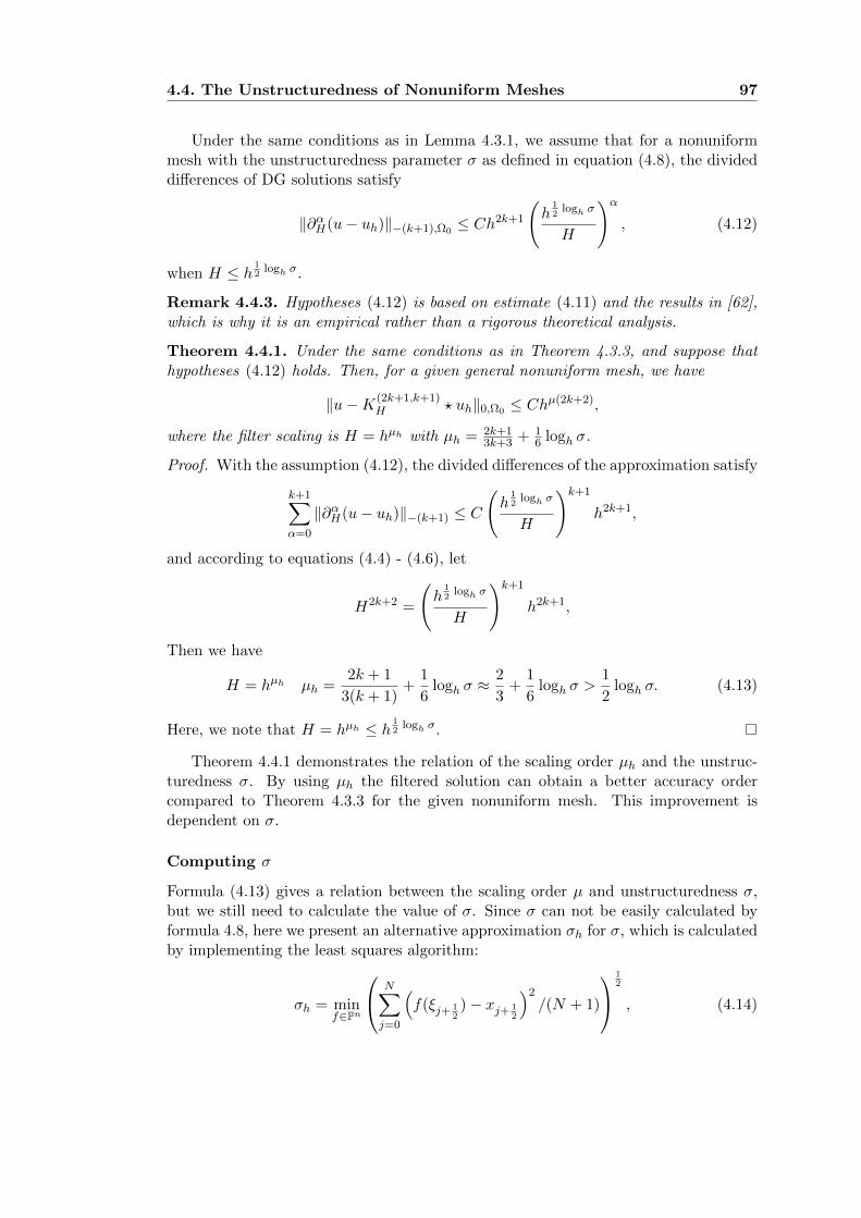
4.4. The Unstructuredness of Nonuniform Meshes 97
Under the same conditions as in Lemma 4.3.1, we assume that for a nonuniformmesh with the unstructuredness parameter σ as defined in equation (4.8), the divideddifferences of DG solutions satisfy
‖∂αH(u− uh)‖−(k+1),Ω0≤ Ch2k+1
(h
12logh σ
H
)α
, (4.12)
when H ≤ h12logh σ.
Remark 4.4.3. Hypotheses (4.12) is based on estimate (4.11) and the results in [62],which is why it is an empirical rather than a rigorous theoretical analysis.
Theorem 4.4.1. Under the same conditions as in Theorem 4.3.3, and suppose thathypotheses (4.12) holds. Then, for a given general nonuniform mesh, we have
‖u−K(2k+1,k+1)H ? uh‖0,Ω0 ≤ Chµ(2k+2),
where the filter scaling is H = hµh with µh = 2k+13k+3 + 1
6 logh σ.
Proof. With the assumption (4.12), the divided differences of the approximation satisfy
k+1∑α=0
‖∂αH(u− uh)‖−(k+1) ≤ C
(h
12logh σ
H
)k+1
h2k+1,
and according to equations (4.4) - (4.6), let
H2k+2 =
(h
12logh σ
H
)k+1
h2k+1,
Then we have
H = hµh µh =2k + 1
3(k + 1)+
1
6logh σ ≈
2
3+
1
6logh σ >
1
2logh σ. (4.13)
Here, we note that H = hµh ≤ h12logh σ.
Theorem 4.4.1 demonstrates the relation of the scaling order µh and the unstruc-turedness σ. By using µh the filtered solution can obtain a better accuracy ordercompared to Theorem 4.3.3 for the given nonuniform mesh. This improvement isdependent on σ.
Computing σ
Formula (4.13) gives a relation between the scaling order µ and unstructuredness σ,but we still need to calculate the value of σ. Since σ can not be easily calculated byformula 4.8, here we present an alternative approximation σh for σ, which is calculatedby implementing the least squares algorithm:
σh = minf∈Pn
N∑j=0
(f(ξj+ 1
2)− xj+ 1
2
)2/(N + 1)
12
, (4.14)

98 Chapter 4. SIAC Filters over Nonuniform Meshes
where
f(x) = anxn + an−1x
n−1 + · · ·+ a1x+ a0,
and
a0a1...an
= A−1
N∑j=0
xj+ 12
(ξj+ 1
2
)0N∑j=0
xj+ 12
(ξj+ 1
2
)1...
N∑j=0
xj+ 12
(ξj+ 1
2
)n
,
with
A =
N∑j=0
(ξj+ 1
2
)0 N∑j=0
(ξj+ 1
2
)1· · ·
N∑j=0
(ξj+ 1
2
)nN∑j=0
(ξj+ 1
2
)1 N∑j=0
(ξj+ 1
2
)2· · ·
N∑j=0
(ξj+ 1
2
)n+1
...... · · ·
...N∑j=0
(ξj+ 1
2
)n N∑j=0
(ξj+ 1
2
)n+1· · ·
N∑j=0
(ξj+ 1
2
)2n
.
Remark 4.4.4. We note that the condition f ′ > 0 in formula 4.8 is usually satisfiedby requiring n N .
In order to give an idea of the computational cost of this algorithm, we presentthe CPU time of calculating σh with different n and N in Table 4.7. The CPU timeis given by the average of 10000 times computation, using quadruple precision. Thecomputational environment is a Intel(R) Core(TM)2 Duo CPU E8500 @3.16GHZ, IntelFortran compiler 9.1. Table 4.7 shows that the computational cost of calculating σh is
Table 4.7: The CPU time (seconds) of calculating σh with polynomials of degreen = 2, 3, 4, 5, 6 for N = 20, 40, 80, 160.
time n = 2 n = 3 n = 4 n = 5 n = 6N = 20 5.08e-5 6.40e-5 7.88e-5 9.48e-5 1.13e-4N = 40 8.68e-5 1.12e-4 1.38e-4 1.66e-4 2.00e-4N = 80 1.58e-4 2.05e-4 2.57e-4 3.09e-4 3.71e-4N = 160 3.00e-4 3.91e-4 4.93e-4 5.90e-4 7.12e-4
negligible.
Table 4.3 gives the values of σh for different nonuniform meshes with differentnumber of elements N . Also, we calculate the value of µh by formula (4.13) andcompare it with the value of µ? given in Table 4.3. Since we obtain σh from equation(4.14), it is a little larger than σ in equation (4.8), and µh is little smaller than theoptimal scaling order. The numerical experiments using µh will be presented in thenext section.

4.4. The Unstructuredness of Nonuniform Meshes 99
Table 4.8: The value of logh σh and µh (4.13) with three different nonuniform meshesof domain Ω = [0, 1]: structured meshes (4.7) with f(ξ) = ξ + 0.1 · sin(2πξ), Mesh3.3.1 and Mesh 3.3.2. Here we use a polynomial of degree n = 8 in the least squaresalgorithm (4.14).
Structured Mesh 3.3.1 Mesh 3.3.2N logh σh logh σh µh: P2,P3 µ?: P2,P3 logh σh µh: P2,P3 µ?: P2,P3
20 3.65 1.53 0.81 0.84 0.90 0.97 1.49 0.80 0.83 0.82 0.9040 2.96 1.40 0.79 0.82 0.85 0.91 1.29 0.77 0.80 0.81 0.8780 2.50 1.33 0.78 0.81 0.84 0.88 1.15 0.75 0.78 0.82 0.85160 2.17 1.30 0.77 0.80 0.81 0.86 1.09 0.74 0.76 0.75 0.80
Correction of Formula (4.13)
In the previous analysis, we used formula (4.13) to calculate the scaling H. However,using formula (4.13) the scaling order µh is still smaller than the optimal scaling orderµ? (see Table 4.8) because when we obtain (4.13), we have not consider the effects ofthe constants in (4.5) and (4.6) which do not depend on the nonuniform mesh. Ignoringthe constants is not a problem if we consider only the accuracy order, but if we wantto achieve the optimal accuracy and make a better approximation, we have to takethese constants into account as well. Here, we propose an alternative that accountsfor the effect of the exact solution:
H = m · hµ µ =2k + 1
3(k + 1)+
1
6logh σ ≈
2
3+
1
6logh σ, (4.15)
where m depends on the exact solution u, more precisely, m = C(|u|
H2k+2
|u|Hk+1
) 13k+3
.
Usually |u|H2k+2 < |u|Hk+1 so that the value of m is usually < 1. In other words, wecan also write (4.15) as
H = hµ µ =2k + 1
3(k + 1)+
1
6logh σ ≈
2
3+
1
6logh σ + loghm. (4.16)
The optimal scaling order is decided by three parts: the basic order, µ0 = 2k+13(k+1) , the
effect of the mesh, 16 logh σ, and the effect of the exact solution. The first two parts
are calculable, but the third is usually decided by experience in practice. For example,we know that the exact solution of Table 4.3 is sin(2π(x − T )). We can considerthe m to be (π)−1/3 to obtain a more precise result. However, in order to avoid thismanufactured aspect, we do not consider m in the following examples.
Remark 4.4.5. It is possible that the optimal scaling H < h, if the mesh is nearlystructured or a structured mesh. In fact, if we consider a wave function sin(λπ) for uni-form meshes, the optimal scaling is much smaller than h when λ is large, see Chapter6.
4.4.3 A Note on Computation
Aside from error reduction, the computational cost of using the filter is also an impor-tant factor in practical applications. As mentioned in previous sections, the scaling
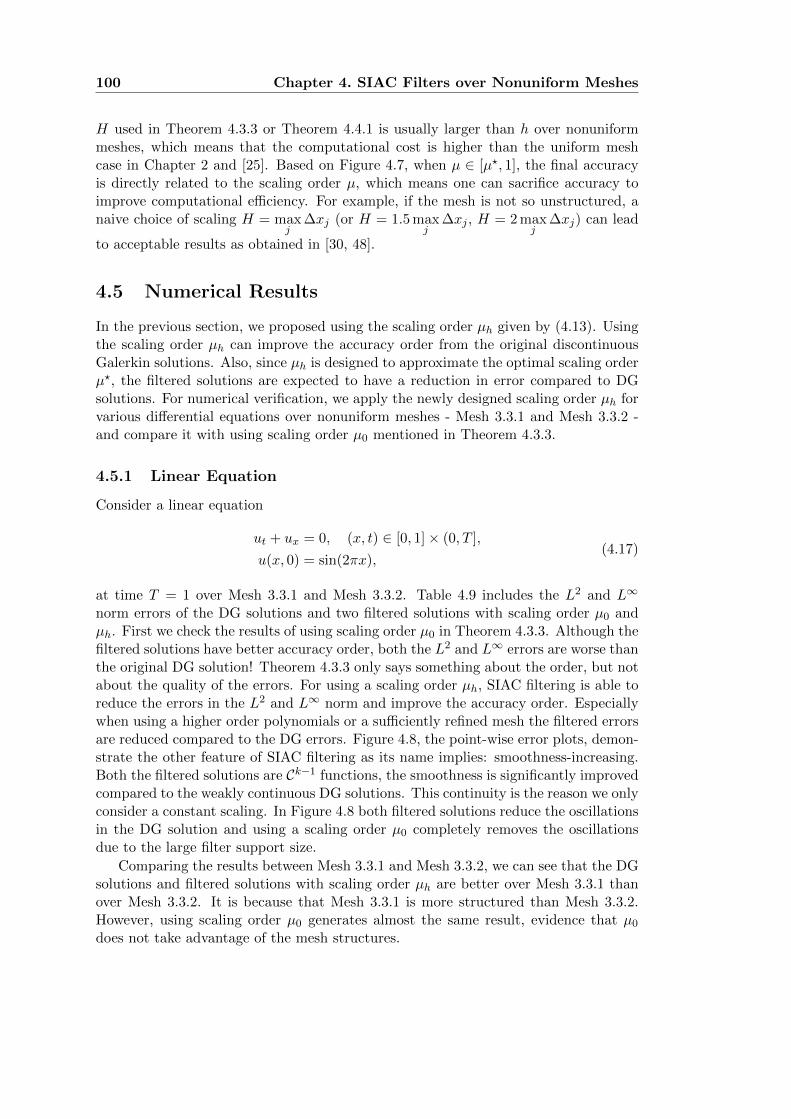
100 Chapter 4. SIAC Filters over Nonuniform Meshes
H used in Theorem 4.3.3 or Theorem 4.4.1 is usually larger than h over nonuniformmeshes, which means that the computational cost is higher than the uniform meshcase in Chapter 2 and [25]. Based on Figure 4.7, when µ ∈ [µ?, 1], the final accuracyis directly related to the scaling order µ, which means one can sacrifice accuracy toimprove computational efficiency. For example, if the mesh is not so unstructured, anaive choice of scaling H = max
j∆xj (or H = 1.5max
j∆xj , H = 2max
j∆xj) can lead
to acceptable results as obtained in [30, 48].
4.5 Numerical Results
In the previous section, we proposed using the scaling order µh given by (4.13). Usingthe scaling order µh can improve the accuracy order from the original discontinuousGalerkin solutions. Also, since µh is designed to approximate the optimal scaling orderµ?, the filtered solutions are expected to have a reduction in error compared to DGsolutions. For numerical verification, we apply the newly designed scaling order µh forvarious differential equations over nonuniform meshes - Mesh 3.3.1 and Mesh 3.3.2 -and compare it with using scaling order µ0 mentioned in Theorem 4.3.3.
4.5.1 Linear Equation
Consider a linear equation
ut + ux = 0, (x, t) ∈ [0, 1]× (0, T ],
u(x, 0) = sin(2πx),(4.17)
at time T = 1 over Mesh 3.3.1 and Mesh 3.3.2. Table 4.9 includes the L2 and L∞
norm errors of the DG solutions and two filtered solutions with scaling order µ0 andµh. First we check the results of using scaling order µ0 in Theorem 4.3.3. Although thefiltered solutions have better accuracy order, both the L2 and L∞ errors are worse thanthe original DG solution! Theorem 4.3.3 only says something about the order, but notabout the quality of the errors. For using a scaling order µh, SIAC filtering is able toreduce the errors in the L2 and L∞ norm and improve the accuracy order. Especiallywhen using a higher order polynomials or a sufficiently refined mesh the filtered errorsare reduced compared to the DG errors. Figure 4.8, the point-wise error plots, demon-strate the other feature of SIAC filtering as its name implies: smoothness-increasing.Both the filtered solutions are Ck−1 functions, the smoothness is significantly improvedcompared to the weakly continuous DG solutions. This continuity is the reason we onlyconsider a constant scaling. In Figure 4.8 both filtered solutions reduce the oscillationsin the DG solution and using a scaling order µ0 completely removes the oscillationsdue to the large filter support size.
Comparing the results between Mesh 3.3.1 and Mesh 3.3.2, we can see that the DGsolutions and filtered solutions with scaling order µh are better over Mesh 3.3.1 thanover Mesh 3.3.2. It is because that Mesh 3.3.1 is more structured than Mesh 3.3.2.However, using scaling order µ0 generates almost the same result, evidence that µ0does not take advantage of the mesh structures.

4.5. Numerical Results 101
Table 4.9: L2− and L∞−errors for the DG approximation uh together two filteredsolutions (using scaling order µ = µ0 and µ = µh) for linear equation (4.17) over Mesh3.3.1 and Mesh 3.3.2
uh µ = µ0 µ = µh
Mesh L2 error order L∞ error order L2 error order L∞ error order L2 error order L∞ error order
Mesh 3.3.1 P1
20 7.59E-03 – 3.00E-02 – 2.91E-02 – 4.12E-02 – 4.95E-03 – 8.26E-03 –40 1.87E-03 2.02 9.51E-03 1.66 7.47E-03 1.96 1.06E-02 1.96 7.19E-04 2.78 1.35E-03 2.6180 4.17E-04 2.16 2.23E-03 2.10 1.88E-03 1.99 2.66E-03 1.99 9.10E-05 2.98 1.86E-04 2.87160 1.00E-04 2.06 5.95E-04 1.90 4.74E-04 1.99 6.71E-04 1.99 1.23E-05 2.89 2.67E-05 2.80
P2
20 2.62E-04 – 1.64E-03 – 5.13E-03 – 7.25E-03 – 7.19E-05 – 1.11E-04 –40 3.26E-05 3.00 2.36E-04 2.80 5.86E-04 3.13 8.29E-04 3.13 3.97E-06 4.18 6.03E-06 4.2180 3.23E-06 3.34 2.11E-05 3.49 6.21E-05 3.24 8.79E-05 3.24 1.99E-07 4.32 2.90E-07 4.38160 4.03E-07 3.00 4.01E-06 2.39 6.36E-06 3.29 8.99E-06 3.29 9.23E-09 4.43 1.40E-08 4.37
P3
20 7.31E-06 – 4.16E-05 – 1.08E-03 – 1.52E-03 – 3.17E-06 – 4.50E-06 –40 5.23E-07 3.80 3.23E-06 3.68 5.17E-05 4.38 7.31E-05 4.38 6.03E-08 5.72 8.72E-08 5.6980 2.64E-08 4.31 1.60E-07 4.33 2.22E-06 4.54 3.14E-06 4.54 9.97E-10 5.92 1.49E-09 5.87160 1.58E-09 4.07 1.16E-08 3.79 9.10E-08 4.61 1.29E-07 4.61 1.42E-11 6.13 2.44E-11 5.93
Mesh 3.3.2 P1
20 1.00E-02 – 3.12E-02 – 3.16E-02 – 4.46E-02 – 7.90E-03 – 1.19E-02 –40 1.99E-03 2.34 1.03E-02 1.60 7.60E-03 2.06 1.07E-02 2.05 9.35E-04 3.08 1.58E-03 2.9180 6.38E-04 1.64 3.99E-03 1.37 1.90E-03 2.00 2.70E-03 1.99 1.41E-04 2.73 2.87E-04 2.46160 1.43E-04 2.15 1.06E-03 1.92 4.79E-04 1.99 6.80E-04 1.99 2.38E-05 2.56 5.00E-05 2.52
P2
20 8.01E-04 – 5.52E-03 – 5.15E-03 – 7.28E-03 – 1.25E-04 – 2.98E-04 –40 6.30E-05 3.67 5.42E-04 3.35 5.87E-04 3.13 8.30E-04 3.13 6.27E-06 4.32 1.14E-05 4.7080 3.86E-06 4.03 2.67E-05 4.35 6.22E-05 3.24 8.79E-05 3.24 4.35E-07 3.85 6.50E-07 4.14160 1.43E-06 1.44 2.23E-05 0.26 6.36E-06 3.29 8.99E-06 3.29 3.18E-08 3.78 1.44E-07 2.17
P3
20 2.07E-05 – 1.17E-04 – 1.08E-03 – 1.52E-03 – 3.80E-06 – 5.99E-06 –40 9.49E-07 4.45 7.44E-06 3.97 5.17E-05 4.38 7.31E-05 4.38 1.03E-07 5.20 1.47E-07 5.3580 7.12E-08 3.74 5.57E-07 3.74 2.22E-06 4.54 3.14E-06 4.54 2.84E-09 5.18 4.22E-09 5.12160 5.77E-09 3.63 6.75E-08 3.04 9.10E-08 4.61 1.29E-07 4.61 5.98E-11 5.57 1.07E-10 5.30
4.5.2 Variable Coefficient Equation
After the linear equation (4.17), which has a constant coefficient, we consider thevariable coefficient equation
ut + (au)x = f, (x, t) ∈ [0, 1]× (0, T ]
u(x, 0) = sin(2πx),(4.18)
where the variable coefficient a(x, t) = 2+sin(2π(x+ t)) and the right side term f(x, t)is chosen to make the exact solution be u(x, t) = sin(2π(x− t)).
Similar to the linear equation example, we compare the L2 and L∞ norm errorsin Table 4.10, and the point-wise error plots are given in Figure 4.9. The results aresimilar to the previous results for the constant coefficient equation. Here we only pointout the features that are different to the linear equation. Using a scaling order µ0 doesnot reliably reduce the errors in the L2 norm and the L∞ norm errors are still worsethan the DG solutions. However, using a scaling order µh reduces the errors in the L2
norm and the L∞ norm. The point-wise error plots in Figure 4.9 are more oscillatorycompared to Figure 4.8 due to the effects of the variable coefficient.
102 Chapter 4. SIAC Filters over Nonuniform Meshes
DG µ = µ0 µ = µhMesh 3.3.1
0 0.2 0.4 0.6 0.8 1.0
x
10−12
10−10
10−8
10−6
10−4
10−2
|erro
r|
N = 20N = 40N = 80N = 160
0 0.2 0.4 0.6 0.8 1.0
x
10−12
10−10
10−8
10−6
10−4
10−2
|erro
r|
N = 20N = 40N = 80N = 160
0 0.2 0.4 0.6 0.8 1.0
x
10−12
10−10
10−8
10−6
10−4
10−2
|erro
r|
N = 20N = 40N = 80N = 160
Mesh 3.3.2
0 0.2 0.4 0.6 0.8 1.0
x
10−12
10−10
10−8
10−6
10−4
10−2
|erro
r|
N = 20N = 40N = 80N = 160
0 0.2 0.4 0.6 0.8 1.0
x
10−12
10−10
10−8
10−6
10−4
10−2|er
ror|
N = 20N = 40N = 80N = 160
0 0.2 0.4 0.6 0.8 1.0
x
10−12
10−10
10−8
10−6
10−4
10−2
|erro
r|
N = 20N = 40N = 80N = 160
Figure 4.8: Comparison of the point-wise errors in log scale of the DG approximationtogether with two filtered solutions (using scaling order µ = µ0 and µ = µh) for linearequation (4.17) over Mesh 3.3.1 and Mesh 3.3.2 with polynomial of degree k = 2.
4.5.3 Two-Dimensional Example
For the two-dimensional example, we consider a two-dimensional linear equation
ut + ux + uy = 0, (x, y) ∈ [0, 1]× [0, 1],
u(x, y, 0) = sin(2π(x+ y)),(4.19)
at time T = 1 over a two-dimensional quadrilateral extension of Mesh 3.3.1 and Mesh3.3.2.
The L2 and L∞ norm errors are presented in Table 4.11 and Table 4.12, the point-wise error plots (pcolor plots) are included in Figure 4.10 and Figure 4.11. The resultsare very similar to the one-dimensional examples: the filtered solutions with scalingorder µh reduce the errors in the L2 norm; using a scaling order µ0 increases the errorin the L2 norm over the DG error. In the two-dimensional case, the computationalefficiency becomes more important compared to the one-dimensional case due the in-creased computational cost. As mentioned before, using a scaling order µ0 is far moreinefficient compared to using the scaling order µh. In particular, for a P3 polynomialbasis with N = 160× 160 meshes, using a scaling order µ0 is more than 8 times slowerover Mesh 3.3.1 (5 times slower over Mesh 3.3.2) than using the scaling order µh.

4.6. Conclusion 103
Table 4.10: L2− and L∞−errors for the DG approximation uh together two filteredsolutions (using scaling order µ = µ0 and µ = µh) for variable coefficient equation(4.18) over Mesh 3.3.1 and Mesh 3.3.2.
uh µ = µ0 µ = µh
Mesh L2 error order L∞ error order L2 error order L∞ error order L2 error order L∞ error order
Mesh 3.3.1 P1
20 6.93E-03 – 3.51E-02 – 2.50E-02 – 3.57E-02 – 1.61E-03 – 4.04E-03 –40 1.83E-03 1.92 1.05E-02 1.74 6.83E-03 1.87 9.71E-03 1.88 2.32E-04 2.79 5.47E-04 2.8980 4.15E-04 2.14 2.29E-03 2.20 1.82E-03 1.91 2.58E-03 1.91 3.72E-05 2.64 1.37E-04 2.00160 1.00E-04 2.05 6.10E-04 1.91 4.66E-04 1.96 6.60E-04 1.97 6.00E-06 2.63 2.09E-05 2.71
P2
20 2.67E-04 – 1.71E-03 – 5.12E-03 – 7.25E-03 – 7.02E-05 – 1.32E-04 –40 3.26E-05 3.03 2.25E-04 2.93 5.86E-04 3.13 8.29E-04 3.13 3.81E-06 4.20 6.82E-06 4.2780 3.24E-06 3.33 2.11E-05 3.42 6.21E-05 3.24 8.79E-05 3.24 1.99E-07 4.26 3.23E-07 4.40160 4.05E-07 3.00 4.01E-06 2.39 6.36E-06 3.29 8.99E-06 3.29 1.03E-08 4.27 2.78E-08 3.54
P3
20 7.43E-06 – 3.68E-05 – 1.08E-03 – 1.52E-03 – 3.18E-06 – 4.75E-06 –40 5.25E-07 3.82 3.14E-06 3.55 5.17E-05 4.38 7.31E-05 4.38 6.07E-08 5.71 1.05E-07 5.5080 2.65E-08 4.31 1.56E-07 4.33 2.22E-06 4.54 3.14E-06 4.54 1.01E-09 5.91 1.73E-09 5.93160 1.58E-09 4.07 1.14E-08 3.78 9.10E-08 4.61 1.29E-07 4.61 1.53E-11 6.04 3.58E-11 5.59
Mesh 3.3.2 P1
20 9.59E-03 – 4.42E-02 – 2.13E-02 – 3.00E-02 – 3.93E-03 – 7.08E-03 –40 1.95E-03 2.30 1.14E-02 1.96 6.77E-03 1.65 9.62E-03 1.64 3.86E-04 3.35 1.09E-03 2.7080 6.38E-04 1.61 4.19E-03 1.44 1.82E-03 1.90 2.60E-03 1.89 8.86E-05 2.12 2.85E-04 1.93160 1.43E-04 2.15 1.09E-03 1.94 4.64E-04 1.97 6.60E-04 1.98 1.65E-05 2.42 5.72E-05 2.32
P2
20 7.90E-04 – 4.96E-03 – 5.08E-03 – 7.19E-03 – 1.71E-04 – 5.14E-04 –40 6.33E-05 3.64 5.08E-04 3.29 5.86E-04 3.12 8.29E-04 3.12 8.54E-06 4.32 2.74E-05 4.2380 3.88E-06 4.03 2.59E-05 4.29 6.21E-05 3.24 8.79E-05 3.24 4.40E-07 4.28 8.34E-07 5.04160 1.44E-06 1.42 2.15E-05 0.27 6.36E-06 3.29 8.99E-06 3.29 1.28E-07 1.78 5.14E-07 0.70
P3
20 2.13E-05 – 1.12E-04 – 1.08E-03 – 1.52E-03 – 4.10E-06 – 8.22E-06 –40 9.62E-07 4.47 6.98E-06 4.01 5.17E-05 4.38 7.31E-05 4.38 1.08E-07 5.24 2.02E-07 5.3580 7.22E-08 3.74 5.24E-07 3.74 2.22E-06 4.54 3.14E-06 4.54 2.94E-09 5.20 5.31E-09 5.25160 5.79E-09 3.64 6.05E-08 3.11 9.10E-08 4.61 1.29E-07 4.61 1.89E-10 3.96 9.78E-10 2.44
4.6 Conclusion
In this chapter, in order to apply a SIAC filter to DG solutions over nonuniformmeshes, we have proposed implementing the filter with a scaling H = hµh . The scalingorder µh is chosen according to the unstructuredness of the given nonuniform mesh.We have proved that by using the scaling H = hµh with µh given in Theorem 4.4.1,the filtered solutions have an accuracy order of µh(2k + 2), which is higher than theaccuracy order of the DG solutions. In addition, since the scaling order µh is designedto approach the optimal scaling order µ?, which minimizes the errors of the filteredsolutions, the error reduction after filtering can be expected. The numerical results arepromising: compared to the original DG errors, the filtered error (with scaling orderµh) has significantly increased the accuracy as well as the accuracy order. Future workwill concentrate on extending this scaling order µh to unstructured triangular meshesin two dimensions and tetrahedral meshes in three dimensions.

104 Chapter 4. SIAC Filters over Nonuniform Meshes
DG µ = µ0 µ = µhMesh 3.3.1
0 0.2 0.4 0.6 0.8 1.0
x
10−12
10−10
10−8
10−6
10−4
10−2
|erro
r|
N = 20N = 40N = 80N = 160
0 0.2 0.4 0.6 0.8 1.0
x
10−12
10−10
10−8
10−6
10−4
10−2
|erro
r|
N = 20N = 40N = 80N = 160
0 0.2 0.4 0.6 0.8 1.0
x
10−12
10−10
10−8
10−6
10−4
10−2
|erro
r|
N = 20N = 40N = 80N = 160
Mesh 3.3.2
0 0.2 0.4 0.6 0.8 1.0
x
10−12
10−10
10−8
10−6
10−4
10−2
|erro
r|
N = 20N = 40N = 80N = 160
0 0.2 0.4 0.6 0.8 1.0
x
10−12
10−10
10−8
10−6
10−4
10−2
|erro
r|
N = 20N = 40N = 80N = 160
0 0.2 0.4 0.6 0.8 1.0
x
10−12
10−10
10−8
10−6
10−4
10−2
|erro
r|
N = 20N = 40N = 80N = 160
Figure 4.9: Comparison of the point-wise errors in log scale of the DG approximationtogether with two filtered solutions (using scaling order µ = µ0 and µ = µh) for variablecoefficient equation (4.17) over Mesh 3.3.1 and Mesh 3.3.2 with polynomial of degreek = 2
DG µ = µ0 µ = µh
Figure 4.10: Comparison of the point-wise errors in log scale of the DG approximationtogether with two filtered solutions (using scaling order µ = µ0 and µ = µh) fortwo-dimensional linear equation (4.19) over Mesh 3.3.1 (2D, P2 and N = 160× 160).

4.6. Conclusion 105
Table 4.11: L2− and L∞−errors for the DG approximation uh together two filteredsolutions (using scaling order µ = µ0 and µ = µh) for two-dimensional linear equation(4.19) over Mesh 3.3.1 (2D).
DG µ = µ0 µ = µh
Mesh L2 error order L∞ error order L2 error order L∞ error order L2 error order L∞ error orderP1
20× 20 1.28E-02 – 6.09E-02 – 5.76E-02 – 8.20E-02 – 1.08E-02 – 1.86E-02 –40× 40 2.57E-03 2.31 1.86E-02 1.71 1.48E-02 1.96 2.11E-02 1.96 1.39E-03 2.96 2.55E-03 2.8780× 80 5.79E-04 2.15 4.94E-03 1.91 3.76E-03 1.98 5.33E-03 1.98 1.80E-04 2.94 3.62E-04 2.81160× 160 1.42E-04 2.03 1.26E-03 1.98 9.48E-04 1.99 1.34E-03 1.99 2.50E-05 2.85 5.27E-05 2.78
P2
20× 20 3.92E-04 – 3.19E-03 – 1.02E-02 – 1.45E-02 – 1.59E-04 – 2.37E-04 –40× 40 4.46E-05 3.13 4.85E-04 2.72 1.17E-03 3.12 1.66E-03 3.12 7.81E-06 4.34 1.19E-05 4.3280× 80 5.09E-06 3.13 5.29E-05 3.20 1.24E-04 3.24 1.76E-04 3.24 3.76E-07 4.38 5.69E-07 4.38160× 160 6.27E-07 3.02 7.49E-06 2.82 1.27E-05 3.29 1.80E-05 3.29 1.89E-08 4.31 3.22E-08 4.14
P3
20× 20 1.18E-05 – 8.74E-05 – 2.15E-03 – 3.04E-03 – 7.21E-06 – 1.03E-05 –40× 40 6.63E-07 4.16 6.65E-06 3.72 1.03E-04 4.38 1.46E-04 4.38 1.19E-07 5.92 1.74E-07 5.8980× 80 3.67E-08 4.17 4.03E-07 4.04 4.44E-06 4.54 6.28E-06 4.54 1.83E-09 6.02 2.82E-09 5.94160× 160 2.24E-09 4.04 2.53E-08 3.99 1.82E-07 4.61 2.57E-07 4.61 2.95E-11 5.96 5.08E-11 5.80
Table 4.12: L2− and L∞−errors for the DG approximation uh together two filteredsolutions (using scaling order µ = µ0 and µ = µh) for two-dimensional linear equation(4.19) over Mesh 3.3.2 (2D).
DG µ = µ0 µ = µh
Mesh L2 error order L∞ error order L2 error order L∞ error order L2 error order L∞ error orderP1
20× 20 2.11E-02 – 1.72E-01 – 6.29E-02 – 9.05E-02 – 1.72E-02 – 3.69E-02 –40× 40 5.44E-03 1.96 6.98E-02 1.30 1.60E-02 1.97 2.32E-02 1.97 3.04E-03 2.50 9.63E-03 1.9480× 80 1.18E-03 2.21 1.42E-02 2.29 3.90E-03 2.04 5.59E-03 2.05 4.00E-04 2.93 1.17E-03 3.04160× 160 2.18E-04 2.43 2.90E-03 2.30 9.57E-04 2.03 1.36E-03 2.04 4.80E-05 3.06 1.11E-04 3.40
P2
20× 20 1.03E-03 – 7.74E-03 – 1.03E-02 – 1.45E-02 – 2.53E-04 – 5.66E-04 –40× 40 1.94E-04 2.41 2.17E-03 1.84 1.18E-03 3.13 1.67E-03 3.13 2.34E-05 3.43 8.41E-05 2.7580× 80 1.97E-05 3.30 3.55E-04 2.61 1.24E-04 3.24 1.76E-04 3.24 1.08E-06 4.44 5.13E-06 4.04160× 160 1.47E-06 3.74 2.77E-05 3.68 1.27E-05 3.29 1.80E-05 3.29 6.07E-08 4.15 1.26E-07 5.35
P3
20× 20 5.18E-05 – 6.23E-04 – 2.15E-03 – 3.04E-03 – 8.67E-06 – 1.63E-05 –40× 40 6.16E-06 3.07 9.20E-05 2.76 1.03E-04 4.38 1.46E-04 4.38 2.75E-07 4.98 1.01E-06 4.0280× 80 2.83E-07 4.44 3.84E-06 4.58 4.44E-06 4.54 6.28E-06 4.54 5.50E-09 5.64 1.57E-08 6.01160× 160 8.38E-09 5.08 1.40E-07 4.78 1.82E-07 4.61 2.57E-07 4.61 1.40E-10 5.30 2.85E-10 5.78
DG µ = µ0 µ = µh
Figure 4.11: Comparison of the point-wise errors in log scale of the DG approximationtogether with two filtered solutions (using scaling order µ = µ0 and µ = µh) fortwo-dimensional linear equation (4.19) over Mesh 3.3.2 (2D, P2 and N = 160× 160).


5Applications of SIAC Filters in the Visualization
In the previous Chapters, we introduced different SIAC filters: symmetric filters, one-sided filters, derivative filters, etc. We demonstrated that by using SIAC filters, onecan improve the results of DG approximation over uniform and nonuniform mesheswith respect to both accuracy and smoothness. In this chapter, we apply SIAC filtersin the visualization area and illustrate that the SIAC filter has great potential in thesepractical applications.
5.1 Introduction
Visualization is concerned with techniques that extract information from the resultsof simulations and computations, such as computational fluid dynamics simulations.The visualization technique is giving a picture to an approximation that helps oneto understand the vector fields resulting from numerical simulations. Given a vectorfield, the streamlines of the field are curves that are tangential to the vector fieldat each point. Streamlines have been demonstrated in much of the literature, suchas [12], to be a powerful and popular visualization method. However, applicationof streamline-based visualization to discontinuous field data represents a significantchallenge due to the discontinuities in the fields. By applying SIAC filters to thediscontinuous data prior to streamline integration, one can overcome the difficultiesof the discontinuous nature of the data. This chapter is aimed at developing goodperformance algorithms of streamline integration by using different SIAC filters thatwere proposed in the previous chapters.
5.1.1 Streamline Integration
For a stationary vector field u, a streamline is an integral curve that is given by theordinary differential equation
dr
dt= u(r), r(t0) = x0. (5.1)
Hence, streamline integration is often accomplished through the application of an or-dinary differential equation (ODE) integrator such as Runge-Kutta (RK) schemes or
107

108 Chapter 5. Applications of SIAC Filters in the Visualization
backward differentiation (BDF) methods. Since the theoretical foundation of theseODE schemes relies on a Taylor expansion, the errors of streamline integration areoften related to the smoothness of the field through which the streamline is beingintegrated.
Discontinuous data fields generated by the finite volume and discontinuous Galerkinmethods are very popular for numerical simulation, such as fluid dynamics simulation.However, calculating streamlines in such discontinuous data field presents a significantchallenge to the classical streamline integration based on the Taylor expansion. Lackingsmoothness at the inter-element level of DG data limits the accuracy of the streamline[61]. In the following sections, we will provide two different ways to use SIAC filtersto enhance the performance of streamline integration over discontinuous data fields.
In this paper, we focus on two-dimensional vector fields with notation
u = [u(x, y), v(x, y)]T , (x, y) ∈ Ω
and the streamlines
r(t) = [x(t), y(t)]T .
5.2 Filtering the Entire Domain
The first method is straightforward and introduced in [61]. First we apply the SIAC fil-ter over the entire domain Ω and obtain a smooth vector field u? = [u?(x, y), v?(x, y)]T ,then uses ODE integrators, such as Runge-Kutta schemes, to calculate the streamline.
More precisely, consider a vector field given by the DG approximation,
u = [u(x, y), v(x, y)]T .
Then the filtered vector field is given by
u? = [u?(x, y), v?(x, y)]T ,
with
u?(x, y) =(u ? K
(2k+1,k+1)h
)(x, y),
v?(x, y) =(v ? K
(2k+1,k+1)h
)(x, y).
Here, the two-dimensional SIAC filter is given by a tensor product of two one-dimensionalfilters that
K(2k+1,k+1)h (x, y) = K
(2k+1,k+1)hx
(x) ·K(2k+1,k+1)hy
(y),
and
u?h(x, y) =
∫R2
K(2k+1,k+1)hx
(x− ξ)K(2k+1,k+1)hy
(y − η)uh(ξ, η)dξdη,
v?h(x, y) =
∫R2
K(2k+1,k+1)hx
(x− ξ)K(2k+1,k+1)hy
(y − η)vh(ξ, η)dξdη.
5.2. Filtering the Entire Domain 109
Remark 5.2.1. In the original work [61], the authors only used the symmetric fil-ter (1.6) in the interior region of the given domain over uniform meshes. Now, withthe new position-dependent filter (2.4) introduced in Chapter 2, and the methods dis-cussed in Chapter 4, we can treat the entire domain over both uniform and nonuniformmeshes.
After filtering the domain, we simply use an explicit Runge-Kutta scheme to cal-culate the streamlines from equation (5.1). More details of Runge-Kutta schemes andtheir error estimations can be found in standard numerical methods textbook, such as[38].
5.2.1 Numerical Results
For the numerical experiments, we consider three analytic fields given in [61], whichhave form:
z = x+ iy,
u = Re(r),
v = −Im(r).
Field 1
r =(z − (0.74 + 0.35i))(z − (0.68− 0.59i))
(z − (−0.11− 0.72i))(z − (−0.58 + 0.64i))
(z − (0.51− 0.27i))(z − (−0.12 + 0.84i))2.
Field 2
r =(z − (0.74 + 0.35i))(z + (−0.18− 0.19i))
(z − (−0.11− 0.72i))(z − (−0.58 + 0.64i))
(z − (0.51− 0.27i)).
Field 3
r =(z − (0.74 + 0.35i))(z − (0.11− 0.11i))2
(z − (−0.11 + 0.72i))(z − (−0.58 + 0.64i))
(z − (0.51− 0.27i)).
The domain of interest is [−1, 1] × [−1, 1] for the above three vector fields. The DGapproximations of these fields are given by the L2 projection onto linear piecewisepolynomial basis functions over a uniform 40 × 40 mesh. Once the approximationfields are obtained, we apply SIAC filters through the entire domain. Here, we pointout that by using the new one-sided filter near the boundaries, we are able to dealwith the entire domain [−1, 1]× [−1, 1] compared to the original results in [61] whichconsidered only the interior region of the domain. For the streamline integration, inthis example we use the second order Runge-Kutta scheme with a time step dt = 0.01.

110 Chapter 5. Applications of SIAC Filters in the Visualization
For convenience, we refer to the streamlines based on the analytic fields to the “exact”streamlines, the streamlines based on the L2 projection fields as DG streamlines, andthe streamlines based on the SIAC filtered fields as filtered streamlines. Streamlineintegration examples based on the given vector fields are presented in Figure 5.1. Notethat in Figure 5.1, the filtered streamline more closely follows the exact streamline.In some cases, one can observe that in regions where bifurcations occur, the filteredstreamline follows the exact streamline, but the DG streamline is diverging away.This behavior can be attributed to enhanced accuracy and smoothness of the filteredapproximation due to applying SIAC filters, and is similar to those found in Steffan etal. [61].
Field 1 Field 2
Field 3
Figure 5.1: Streamlines based upon vector fields: Field 1, Field 2 and Field 3. Blacksolid lines denote the “exact” solution, red dashed lines are the DG streamlines andblue dashed dot lines are the filtered streamlines. Note the black lines are overlappedby the blue lines.
In addition, we use the Hausdorff distance metric to measure the error of theDG streamline and the filtered streamline with respect to the “exact” streamline. TheHausdorff distance is a very popular technique to define a distance between two curves.

5.3. Filtering Along the Streamline 111
Given two curves X and Y , their Hausdorff distance dH(X,Y ) is defined by
d(X,Y ) = max
supx∈X
infy∈Y
d(x, y), supy∈Y
infx∈X
d(x, y)
,
where d(x, y) denotes the standard euclidean distance between two points. Table 5.1presents the Hausdorff distances of the streamlines given in Figure 5.1. In Table 5.1,we observe that the filtered streamlines are close to the exact streamlines compared tothe DG streamlines.
Table 5.1: The error (Hausforff distance) for the DG streamlines and the filteredstreamlines in Figure 5.1.
DGFiltered
line 1 line 2 line 3
Field 12.71E-2
1.28E-3 2.83E-29.80E-3 9.75E-1
1.32E-2
Field 21.37E-0
1.73E-3 2.89E-12.90E-3 7.33E-2
1.83E-3
Field 34.63E-3
4.48E-3 7.71E-34.90E-3 1.00E-1
4.70E-3
5.3 Filtering Along the Streamline
The first streamline integration method demonstrated good performance. However,the algorithm of filtering the entire domain is computationally expensive, especial forhigher dimensional vector fields. In order to develop an alternative efficient algorithm,Walfisch et al. [68] proposed the idea of filtering along the streamline. This idea usesthe information from the streamline instead of information from the entire domain.To implement this idea, one needs to use one-sided filters. In [68], the authors usedthe RS filter (1.12). In this section, we will use the newly defined position-dependentfilter (2.4) which has proved to have better performance than the RS filter.
5.3.1 Backward-Differentiation Methods
In [68], the authors used the 1D one-sided filtering with Runge-Kutta schemes for thestreamline integration. However, we point out these Runge-Kutta schemes requiresampling the field from positions that are not along the streamline. Since the filteringproposed in the algorithm is done along the streamline, evaluating the points whichare not on the streamline is inconsistent. To explain this, we give the formula for thesecond order Runge-Kutta scheme
k1 = hf(tn, yn)
k2 = hf(tn +h
2, yn +
k12)
yn+1 = yn + k2.

112 Chapter 5. Applications of SIAC Filters in the Visualization
In the above formula, it is clear that the point (tn +h2 , yn +
k12 ) in step 2 usually does
not belong to the streamline, and then we can not use filtering at this point along thestreamline. The same thing occurs with any other multi-stage methods.
Also, we want the algorithm to work reasonably well for other integration curves,such as streaklines and pathlines. Based on these reasons, we use backward differenti-ation methods as the integrator for the streamline integration. By choosing backwarddifferentiation for integration, it allows us to use a larger time-step which will beoutside an explicit integrator’s stability region.
Consider the general formula for multi-step schemes and select backward differenti-ation as the time-stepping method, one gets a backward differentiation formula (BDF)of the form
p∑i=0
αirn+1−i = ∆tβun+1
where the coefficients for a fixed time step are given as in Table 5.3.1, see [38].
Table 5.2: Backward Differentiation CoefficientsOrder p β α1 α2 α3 α4
1 1 −12 2
3 −43
13
3 611 −18
11911 − 2
11
4 1225 −48
253625 −16
25325
The standard practice for reaching an order (i.e. p) scheme is to start with ap = 1 scheme and “jump-start” once calculations up through the orders as morepositional data becomes available. In this section, we initiate the time-stepping withthe trapezoidal rule version of the BDF given by:
rn+1 = rn +∆t
(1
2un +
1
2un+1
).
Note that this is an implicit formula and hence requires a root finding technique. In thissection, we use the multi-dimensional Newton’s method which requires us to re-writethe scheme in root finding form as:
g(rn+1) = rn+1 − rn −∆t
(1
2un +
1
2un+1
)= 0.
The goal is to find the Newton’s method iterate (denoted by k) such that g(rn+1,k+1) =0 (or in our case, machine zero).
To implement Newton’s method, we define the Jacobian matrix
Jg(rn+1,k) =
(∂g1∂x
∂g1∂y
∂g2∂x
∂g2∂y
)rn+1,k
and iterate Newton’s formula given by:
rn+1,k+1 = rn+1,k − [Jg(rn+1,k)]−1g(rn+1,k). (5.2)

5.3. Filtering Along the Streamline 113
Once the time-stepping has been initiated, one can work their way up the differentorders p using the following formula:
rn+1 = ∆tβu(rn+1)−p∑
i=1
αirn+1−i.
To be able to solve the multi-dimensional Newton’s method, we do the same methodand construct a function:
g(rn+1) = ∆tβu(rn+1)− rn+1 −p∑
i=1
αirn+1−i = 0.
The goal is to find the Newton’s method iterate (denoted by k) such that g(rn+1,k+1) =0.
5.3.2 Algorithm
To give the complete algorithm of filtering along the streamline, we consider a vectorfield Ω (triangles or quadrilaterals in two-dimension and tetrahedra, hexahedra, prismsor pyramids in three-dimensions).
First, we describe the outline of the algorithm of filtering along the streamline.Once we obtain r0, r1, . . . , rn−1, rn, like Figure 5.2, we can evaluate the new positionrn+1 in the following steps:
1. Construct a streamline based on the known information by using interpolationmethods.
2. Rewrite the streamline from Cartesian coordinates to arc-length coordinates.
3. Apply a one-sided filter along the streamline to obtain a filtered vector field.
4. Use backward-differentiation methods to obtain the new position rn+1.
Figure 5.2: Structure of the algorithm: filtering along the streamline.
The discontinuous Galerkin approximation of the vector filed is given by
u = [u(x, y), v(x, y)]T .
114 Chapter 5. Applications of SIAC Filters in the Visualization
A streamline r(t) = [x(t), y(t)]T of this vector field u is an integration curve thatsatisfies
dr
dt= u(r).
We now present the details of how to filtering along the streamline. To filtering alongthe streamline, we need to consider using the arc-length coordinates instead of theCartesian coordinates as mentioned above.
By considering the arc-length coordinates, we can write the filtered vector field as
u?(r(sn)) = Kh ? u(sn) =
∫ ∞
−∞Kh(sn − s)u(r(s))ds,
where r(sn) is the new position of the streamline. Here, we assume that there is enoughhistory of the data to apply the one-sided filter (2.4) proposed in Chapter 4. Denotethe support of the filter included in segment I1, . . . , In, where Ij = [sj−1, sj ], then wecan rewrite the above formula as
u?(r(sn)) =n∑
j=1
∫Ij
Kh(sn − s)u(r(s))ds.
For each segment Ij , let τ ∈ [0, 1] be the variable which we parameterize the curve, sothat ∫
Ij
Kh(sn − s)u(r(s))ds =∫ 1
0Kh(sn − s(τ))u(rj(τ))
ds
dτdτ.
In each segment Ij , the curve rj(τ) has form
rj(τ) = (x(τ), y(τ)), τ ∈ [0, 1],
and
ds
dτ=
√(dx(τ)
dτ
)2
+
(dy(τ)
dτ
)2
, s(τ) =
∫ τ
0
ds
dτdτ.
In particular, for linear interpolation
rj(τ) = xj−1 + τ(xj − xj−1),
withds
dτ=√(xj − xj−1)2 + (yj − yj−1)2 = ∆sj , s(τ) = ∆sjτ,
then we have ∫Ij
Kh(∆sm−j + sj − s)r(s)ds
=
∫ 1
0Kh(∆sm−j + (1− τ)∆sj)rj(τ)∆sjdτ.
In order to use backward differentiation methods and Newton iteration (5.2), wealso need to calculate the Jacobian matrix
Jg(rn+1,k) =
(∂g1∂x
∂g1∂y
∂g2∂x
∂g2∂y
)rn+1,k
=
(∂u∂x
∂u∂y
∂v∂x
∂v∂y
)rn+1,k
−(
1 00 1
).

5.3. Filtering Along the Streamline 115
Since the above Jacobian matrix includes the derivatives, we also need to use theone-sided derivative filter proposed in Chapter 3. In Chapter 3, the formula of thefiltered solution for αth derivative was given by:
dαu?
dxα=
dα
dxα
(K
(2k+1,k+1+α)h ? u
)=(∂αh K
(2k+1,k+1,α)hT
)? u,
where the filter Kh is one-sided derivative filter, K(2k+1,k+1,α)hT , given in (3.6).
First, we consider the ∂u?
∂x term. The filtered solution is
u?(r(sn)) = Kh ? u(sn).
Using the same notation as in previous steps, we get
∂
∂xu? =
n∑j=1
∫Ij
∂
∂xKk+1+1
h (sn − s)u(r(s))ds
=
n∑j=1
∫Ij
(∂hK
k+1h
)(sn − s)
∂s
∂xu(r(s))ds.
For linear interpolation, we will have
∂
∂xu? =
n∑j=1
∫ 1
0
(∂hK
k+1h
)(sn − s(τ))
ds
dτ
dτ
dxu(rj(τ))
ds
dτdτ
=n∑
j=1
∫ 1
0
(∂hK
k+1h
)(sn − s(τ))u(rj(τ))
(∆sj)2
xj − xj−1dτ.
Similarly, for the remaining three terms,
∂
∂yu? =
n∑j=1
∫ 1
0
(∂hK
k+1h
)(sn − s(τ))u(rj(τ))
(∆sj)2
yj − yj−1dτ
∂
∂xv? =
n∑j=1
∫ 1
0
(∂hK
k+1h
)(sn − s(τ))v(rj(τ))
(∆sj)2
xj − xj−1dτ
∂
∂yv? =
n∑j=1
∫ 1
0
(∂hK
k+1h
)(sn − s(τ))v(rj(τ))
(∆sj)2
yj − yj−1dτ
Remark 5.3.1. The integration can be calculated by using Gauss quadrature, but weneed to consider both the DG breaks and the filter breaks as mentioned in Chapter 1.

116 Chapter 5. Applications of SIAC Filters in the Visualization
5.3.3 Preliminary Results
Time Cost
First, we check the computational cost for the algorithm of filtering along the stream-line and compare it with the method of filtering the entire field. To avoid interruption,we test two algorithms for the simplest vector field, a constant vector field u = [1, 1]T .Then the streamlines will be straight lines, and the numerical approximations shouldbe exactly the same, see Figure 5.3. Also, we provide Table 5.3, which shows the com-putational cost (time) of using these two algorithms. From the table, we can clearlysee that filtering along the streamline can significantly reduce the computational cost,which is almost 70 times faster than filtering the entire field.
Filtering entire domain Filtering along streamline
Figure 5.3: Straight-line streamlines based upon vector field u = [1, 1]T . We notethat the numerical approximations are exact.
Table 5.3: Number of steps, time per integration step and ratio of filtering alongthe streamline to filtering the entire field time per step required to calculate threestreamlines on the constant vector field u = [1, 1]T .
Filtering entire field Filtering along streamline
streamline Steps Time/Step(sec) Steps Time/Step(sec) Ratio
1 190 2.64e-02 190 3.79e-04 69.72
2 120 2.61e-02 120 3.67e-04 71.14
3 120 2.62e-02 120 3.67e-04 71.36
Then, we consider the same three analytic fields used in the previous section. Thedomain is [−1, 1]× [−1, 1], and the DG approximations are given by the L2 projection,polynomial P1, onto a uniform 40×40 mesh. Here, the filtered streamline is obtained byusing the algorithm of filtering along the streamline. For streamline integration, we usethe second order backward-differentiation method with time step dt = 0.01. Streamline

5.3. Filtering Along the Streamline 117
integration examples based the given vector fields are presented in Figure 5.4. UnlikeFigure 5.1, the difference between the filtered streamline and the DG streamline isquite small and hard to observe from the plots (unless zoom in). However, we can stillcompare the error by using the Hausdorff distance. Table 5.4 presents the Hausdorffdistances of the streamlines given in Figure 5.4. From Table 5.1, we observe that thefiltered streamlines are slightly close to the exact streamlines compared to the DGstreamlines, but the advantage is not obvious.
Field 1 Field 2
Field 3
Figure 5.4: Streamlines based upon vector fields: Field 1, Field 2 and Filed 3. Blacksolid lines denote the “exact” solution, red dashed lines are the DG streamlines andblue dashed dot lines are the filtered streamlines. Using one-sided filtering along thestreamline.
Remark 5.3.2. The filtered streamline obtained by applying the method of filteringalong the streamline is less accurate compared to the method of filtering the entiredomain. It is a method to sacrifice accuracy for speed.
Remark 5.3.3. The results presented in this section are only preliminary results. Inorder to obtain optimal results, we must answer the following questions:

118 Chapter 5. Applications of SIAC Filters in the Visualization
Table 5.4: The error (Hausforff distance) for the DG streamlines and the filteredstreamlines in Figure 5.4.
BeforeAfter
line 1 line 2 line 3
Field 14.72E-3
3.49E-3 3.45E-22.37E-3 1.00E-1
9.08E-2
Field 28.09E-2
2.00E-2 2.26E-31.17E-3 5.00E-3
3.34E-3
Field 32.70E-3
4.03E-3 1.54E-28.24E-4 1.85E-2
1.26E-2
• Which method should be used for reconstructing the streamline: linear interpola-tion, Hermite interpolation or others?
• Are backward-differentiation methods the best integration method when filteringalong the streamline?
• Which one-sided filter is the most suitable one for filtering along the streamline?
• How should the filter scaling be chosen for filtering along the streamline? Whenfiltering along the streamline, in order to use the one-dimensional one-sided filter,we must consider arc-length coordinates. It follows that we have to use the filterover a nonuniform mesh. As mentioned in Chapter 4, the choice of the filteringscaling is directly related to the final accuracy.
5.3.4 Which One-Sided Filter?
For filtering along the streamline, one must use a one-sided filter. It follows that aninteresting question is which one-sided filter is the most suitable one for this algorithm.As introduced earlier, there are three one-sided filters: the RS filter (1.12), the SRVfilter (1.14) and the new filter (2.4). In the previous parts of this chapter, we useonly the new filter since the other two filters do not acquire any information at thepoint where the filtered value needs to be computed. However, it is still interesting tocompare the behaviors of using these three one-sided filters for streamline integration.
In Figure 5.5 and Table 5.5, we compare the results of using these three one-sidedfilters over Field 2. One can observe that the new filter provides the most accurateresults, then the RS filter. For the SRV filter, the results are significantly worse thanthe other two one-sided filters and the DG solutions.
Table 5.5: The error (Hausforff distance) for the DG streamlines and the filteredstreamlines with three different one-sided filters in Figure 5.5.
DG RS filter SRV filter New filterline 1 8.09E-2 6.71E-2 5.11E-2 2.00E-2line 2 2.26E-3 1.41E-3 2.21E-1 1.17E-3line 3 5.00E-3 3.61E-3 4.36E-2 3.34E-3

5.3. Filtering Along the Streamline 119
RS filter SRV filter
New filter
Figure 5.5: Streamlines based upon Field 2. Black solid lines denote the “exact”solution, red dashed lines are the DG streamlines and blue dashed dot lines are thefiltered streamlines. Using three different one-sided filters.
Then, we consider an interesting field given by [68] which was defined in polarcoordinates by [
u(r, θ)v(r, θ)
]=
[12 cos(20θ) cos(θ)− r sin(θ)12 cos(20θ) sin(θ) + r cos(θ)
]. (5.3)
This field has streamlines which are oscillating closed circuits. In [68], the authorcompared the results of the DG streamline and the filtered streamline with using theRS filter, see Figure 5.6.
In order to compare the results of using different one-sided filters, we redo theexample with the same settings by using SRV filter (1.14) and the new filter (2.4), seeFigure 5.7. Comparing the results in Figures 5.6 and 5.7, the new filter is still thewinner. However, we point out the results of using the RS filter are also acceptable,and the SRV filter is diverging away from the actual streamline. Through the aboveexamples, we can clearly see that for filtering along the streamline one can use eitherthe new filter or the RS filter, but the SRV filter is not a suitable choice.

120 Chapter 5. Applications of SIAC Filters in the Visualization
Figure 5.6: Streamline integrations [68] based upon vector field (5.3). Using the RSfilter.
SRV filter new filter
Figure 5.7: Streamline integrations based upon vector field (5.3). Black solid linesdenote the “exact” solution and red dashed dot lines are the filtered streamlines. Usingthe SRV filter and the new filter.
5.4 Conclusion
The SIAC filtering technique has demonstrated its ability to improve the continuityof the discontinuous Galerkin solution and maintain the accuracy. Therefore, SIACfiltering has potential value as a preprocessing tool prior to other techniques such asvisualization techniques. In this chapter, we presented the preliminary results of apply-ing SIAC filters for streamline visualization. We briefly discussed how to apply SIACfilters for the discontinuous Galerkin approximations that results in more accurate

5.4. Conclusion 121
streamline placements. There are two ways to use SIAC filters for streamline integra-tion. The first one is using the filter introduced in Chapter 2 to filter the entire vectorfield, and then perform the streamline integration. This method is mature and robust,and the filtered streamlines are closer to the exact streamlines compared to the DGstreamlines. Also, applying SIAC filtering before the streamline integration, to a greatextent, has avoided diverging situations for the streamlines. The second method isproposed based on computational considerations. This method considers filtering onlyalong the streamline rather than the entire domain. Clearly, filtering along the stream-line is more efficient compared to filtering the entire domain. However, as mentionedin this chapter, the method of filtering along the streamline is on-going research, and itis not robust as the method of filtering the entire domain. Through some preliminaryresults, we indicate there are several points that need to be discussed or resolved:
• The first question is: which one-sided filter to use? The algorithm of filteringalong the streamline requires using a one-sided SIAC filter. Based on numer-ical experiments, we point out we should make a choice between the RS filter(1.12) and the new filter (2.4). The SRV filter (1.14) is not a suitable choice forstreamline integration.
• The second question is: how should the filter scaling be chosen? As mentionedin Chapter 4, the filter scaling is the crucial factor for filtering over nonuniformmeshes, and algorithm of filtering along the streamline is always performed overnonuniform meshes no matter the original tessellation.
• There are some remaining details about the implementation of the algorithm,such as which interpolation method to reconstruct the streamline, and whichintegration method for the streamline integration.
If these are solved, this algorithm could be of great value to visualization techniques.Additionally, the idea of this algorithm that is dealing with multi-dimensional data ina one-dimensional operation has great potential value for many other applications.
Further works relate this chapter are:
• Further investigation of the algorithm of filtering along the streamline and de-velop it into a robust algorithm.
• Extend the algorithm to other visualization techniques, such as other integrationcurves (streakline, pathline, etc.).
• Theoretical analysis of the algorithm, such as error estimates.


6Further Inverstigation of SIAC Filter
In Chapter 1, we introduced the original definition and properties of the SIAC filter.In this chapter, we will investigate further details of the SIAC filter and its variations.For convenience, without specification the filters in this chapter are symmetric filters.However, one can easily extend the results in this chapter to one-sided filters.
6.1 Structure of SIAC Filter
In Chapter 1, we discussed the structure of the original symmetric SIAC filter - a linearcombination of central B-splines. Following this construction an interesting questionis: is there another structure that allows one to extract the superconvergence order of2k + 1 from DG solutions?
To answer this question, we recall the necessary components to extract the su-perconvergence order of 2k + 1, Theorem 1.3.4. Through the proof of Theorem 1.3.4given in [25], one can see that there are four main components behind Theorem 1.3.4,namely, Lemma 1.2.2, Theorem 1.2.1, Property 1.3.2 and Property 1.3.3:
• Lemma 1.2.2 shows that the L2 norm of a function can be bounded by thenegative order norm of the derivatives of the same function. It is dependent onthe regularity of the function.
• Theorem 1.2.1 proves that the DG solution and its divided differences have super-convergence order of 2k+1 in the negative order norm. It is the superconvergenceof the DG solution.
• Property 1.3.2 demonstrates that the filter has the ability to reproduce polyno-mials by convolution. It is due to equation (1.8).
• Property 1.3.3 allows us to express derivatives in term of divided difference quo-tients. It is due to the structure of the SIAC filter, more precisely, the centralB-splines.
Through the above analysis, we know the key structure of the filter is to provide theability to express derivatives in term of divided differences. Therefore, the task is to
123

124 Chapter 6. Further Inverstigation of SIAC Filter
find a basis function φ(`), such that
d
dxφ(`)H (x) = ∂Hφ
(`−1)(x) =1
h
(φ(`−1)(x+ h/2)− φ(`−1)(x− h/2)
), (6.1)
then we can construct the filter by
K(2k+1,k+1) =
2k∑γ=0
c(2k+1,k+1)γ φ(k+1)(x− (−k + γ)), (6.2)
where c(2k+1,k+1)γ is decided by (1.8).
In order to find such a basis function φ(`), we take the Fourier transform of equation(6.1)
2πiξφ(`) = φ(`−1)eπiξ − φ(`−1)e−πiξ =⇒ φ(`) = φ(`−1) sin(πξ)
πξ.
It is easy to verify that χ[−1/2,1/2] =sin(πξ)
πξ , then we have
φ(`) = φ(`−1) ? χ[−1/2,1/2]. (6.3)
Once we decide the initial function φ(1), the filter, constructed by (6.2) and (6.3), canextract the superconvergence order of 2k + 1 from the DG solution. The simplestand natural choice is φ(1) = χ[−1/2,1/2], which leads to the central B-spline filter. Of
course, we can choose another initial function, such as φ(1) = cos(πx)χ[−1/2,1/2], φ(k)
with k = 2, 3, 4. These are shown in Figure 6.1.
k = 2 k = 3 k = 4
−1 0 10.0
0.2
0.4
0.6
0.8
1.0
−1.5 −0.5 0.5 1.50.0
0.2
0.4
0.6
0.8
1.0
−2 −1 0 1 20.0
0.2
0.4
0.6
0.8
1.0
Figure 6.1: Basis φ(k), which satisfies (6.3), with φ(1) = cos(πx)χ[−1/2,1/2].
We can see that the filter given in (6.2) constructed by the basis function φ(k+1),which satisfies (6.3), also has Property 1.3.3. Then, the following question is: do there
exist constants c(2k+1,k+1)γ such that filter (6.2) reproduces polynomials by convolution
until degree up to degree 2k? To answer this question, we present Theorem 6.1.1 forthe more general situation.
Theorem 6.1.1. Assume φγ , γ = 0, . . . , r are r + 1 normalized linear independentfunctions, each with has compact support. Then the linear system
r∑γ=0
cγ
∫ ∞
−∞φγ(ξ)(x− ξ)mdξ = xm, m = 0, 1, . . . , r (6.4)

6.1. Structure of SIAC Filter 125
has a unique solution.
Proof. For convenience, we denote that
A(γ,m)(x) =
∫ ∞
−∞φγ(ξ)(x− ξ)mdξ, γ,m = 0, 1, . . . , r,
= xm +
m−1∑j=0
λjγ,mxj ,
where λjγ,m =∫∞−∞ φγ(ξ) (−ξ)j
(mj
)dξ. Then, the conclusion in Theorem 6.1.1 is equiv-
alent to matrix A(γ,m) is nonsingular, in other words, we only need to prove the r+1rows A(γ,m)rγ=0 are linear independent.
Assume there exist constants bm,m = 0, . . . , r such that
r∑m=0
bmA(γ,m)(x) = 0, γ = 0, . . . , r.
By substituting the form of A(γ,m), we have
r∑m=0
bm
xm +m−1∑j=0
λjγ,mxj
= 0 ⇒r∑
m=0
bm +r∑
j=m+1
bjλmγ,i
xm = 0.
Since the above relation is true for all x ∈ R, we know
bm +
r∑j=m+1
bjλmγ,i = 0 ⇒
br = 0br−1 = −λr−1
γ,r br = 0
. . .
b0 = −
(r∑
j=1λ0γ,jbj
)= 0.
.
It follows that the r + 1 rows of linear system (6.4) is linear independent.
Since φ(k+1)(x+k−γ), γ = 0, . . . , r, are r+1 linear independent compact functions,
Theorem 6.1.1 indicates that there exists unique constants c(2k+1,k+1)γ such that filter
(6.2) reproduces polynomials by convolution up to degree 2k. For example, the filterswith φ(1) = cos(πx)χ[−1/2,1/2] are presented in Figure 6.2.
Finally, we know that there are infinitely many structures of the SIAC filter thatallow us to extract the superconvergence order of 2k + 1 from the DG solutions.
Theorem 6.1.2. Under the same conditions in Theorem 1.3.4, the filter given in(6.2), then
‖u−K(2k+1,k+1)h ? uh‖0,Ω0 ≤ Ch2k+1.
Proof. The proof is the same as in Theorem 1.3.4
Here, we point out that if we limit a SIAC filter to be a piecewise polynomial, thenthe original symmetric filter constructed by central B-splines has the simplest formula.

126 Chapter 6. Further Inverstigation of SIAC Filter
k = 1 k = 2 k = 3
−2 −1 0 1 2−0.2
0.0
0.4
0.8
1.2
−4 −3 −2 −1 0 1 2 3 4−0.2
0.0
0.4
0.8
1.2
−5−4−3−2−1 0 1 2 3 4 5−0.2
0.0
0.4
0.8
1.2
Figure 6.2: K(2k+1,k+1) given in (6.2) constructed by basis φ(k+1), which satisfies(6.3), with φ(1) = cos(πx)χ[−1/2,1/2].
Remark 6.1.1. Through the technique discussed in this section, we can create aninfinitely smooth SIAC filter to enhance the smoothness of the filtered solutions. Forexample, we can choose
φ(1) =
exp
(− 1
1−4x2
), |x| < 1
2
0, |x| ≥ 12
.
Then we can obtain a filter which has the same support size as the original filter,but it belongs to C∞0 . It follows that the filtered solution u?h ∈ C∞ and also has accuracyorder of 2k + 1.
6.2 The Order of B-splines
As mentioned in the previous chapters, the order of the SIAC filter plays a very importrole, such as for derivative filters. According to the error estimates, one must use acertain order of B-splines to convert all the required derivatives into divided differences.This is the reason we can not use a linear filter to filter a cubic DG approximations.
6.2.1 The Lowest Order of B-splines
This leads to the following question: what is the lowest order of B-spline that ensuresobtaining accuracy order of 2k + 1. Usually, we choose the order of B-splines to bek + 1, which means the filter K(2k+1,k+1) is a piece-wise polynomial of degree k.
One can verify that the filtered solution, u?h = K(2k+1,k+1)h ? uh, is a piecewise
polynomial of degree 2k+1. Based on the approximation theorem, as a polynomial ofdegree 2k + 1, the filtered solution does not obtain its optimal accuracy order 2k + 2.In fact, due to the superconvergence property of the DG solution, Theorem 1.2.1, theaccuracy order of 2k+2 is usually impossible unless uh is a L2 projection of the exactsolution.
However, it leads to a conjecture that we can use filter K(2k+1,k), order k filter, toapproach the accuracy order of 2k + 1.

6.2. The Order of B-splines 127
Theorem 6.2.1. Under the same conditions in Theorem 1.3.4, then
‖u−K(2k+1,k)h ? uh‖0,Ω0 ≤ Ch2k+1.
Proof. The proof is the same as in Theorem 1.3.4.
Remark 6.2.1. Theorem 6.2.1 also explains the behavior that after using the filterK(2k+1,k+1), the first derivative of the filtered solution has accuracy order 2k + 1 not2k as theorem in [56] suggested.∥∥∥∂xu− ∂x (K(2k+1,k+1)
h ? uh
)∥∥∥0,Ω0
≤ Ch2k+1.
Since K(2k+1,k)h ? uh is only a piecewise polynomial of degree 2k, we can claim that
the accuracy order 2k + 1 is already optimal. Also, the approximation theorem tellsus the order of filter can not be lower than k, and order k is already the lowest order ifan accuracy order of 2k+1 is desired. Now, we compare the differences between usingthe k + 1th order filter and the kth order filter.
Example 6.2.2. Consider a linear hyperbolic equation
ut + ux = 0, (x, t) ∈ [0, 1]× (0, T ]
u(x, 0) = sin(2πx)
with final time T = 1 over uniform meshes. The L2 and L∞ norm errors and respectiveaccuracy order are given in Table 6.1. Figure 6.3 shows the point-wise errors in logscale. The respective results of the DG approximation can be found in Example 1.3.5.
K(2k+1,k+1) K(2k+1,k)
0 0.2 0.4 0.6 0.8 1.0
x
10−16
10−12
10−8
10−4
|erro
r|
N = 20N = 40N = 80N = 160
0 0.2 0.4 0.6 0.8 1.0
x
10−16
10−12
10−8
10−4
|erro
r|
N = 20N = 40N = 80N = 160
Figure 6.3: Comparison of the point-wise errors in log scale of the filtered solutionswith the kth and (k + 1)th symmetric filter. The DG basis are polynomials P3 for alinear advection equation.

128 Chapter 6. Further Inverstigation of SIAC Filter
Table 6.1: L2− and L∞−errors for the filtered solutions u?h with the kth and (k+1)thsymmetric filter for a linear advection equation.
K(2k+1,k+1) K(2k+1,k)
Mesh L2 error order L∞ error order L2 error order L∞ error orderP1
20 1.97E-03 – 2.80E-03 – 1.94E-03 – 2.75E-03 –40 2.44E-04 3.02 3.46E-04 3.02 2.42E-04 3.00 3.44E-04 3.0080 3.02E-05 3.01 4.28E-05 3.01 3.02E-05 3.00 4.29E-05 3.00160 3.76E-06 3.01 5.33E-06 3.01 3.77E-06 3.00 5.35E-06 3.00
P2
20 4.11E-06 – 5.82E-06 – 3.09E-06 – 4.39E-06 –40 9.49E-08 5.44 1.34E-07 5.44 7.88E-08 5.29 1.12E-07 5.2980 2.49E-09 5.25 3.52E-09 5.26 2.24E-09 5.14 3.19E-09 5.14160 7.75E-11 5.00 1.10E-10 5.00 7.38E-11 4.92 1.05E-10 4.93
P3
20 6.97E-08 – 9.86E-08 – 4.15E-08 – 5.87E-08 –40 2.83E-10 7.95 4.00E-10 7.95 1.70E-10 7.93 2.40E-10 7.9380 1.23E-12 7.85 1.73E-12 7.85 7.82E-13 7.76 1.11E-12 7.76160 1.59E-14 6.27 2.25E-14 6.27 1.41E-14 5.79 2.00E-14 5.79
Table 6.1 shows that both the kth and (k + 1)th order filters can give us accuracyorder of 2k+ 1 for the filtered solutions. Here, we point out although the difference isquite small, and the filtered solutions obtain by using the kth order filter have betteraccuracy compared to using the (k+1)th order filter. These results are consistent withstudies in Chapter 4 that with the higher order filter, the optimal scaling is increased.
Figure 6.3 reveals that for high order polynomials, such as P3, the filtered solutionslook almost the same as filters K(2k+1,k) and K(2k+1,k+1). However, if we check theresults for P1 in Figure 6.4, we can see that using the (k + 1)th order filter generatesa smoother result than using the kth order filter.
The conclusion is simple, using kth order filter is computationally more efficientbut the filtered solutions are less smooth compared to using (k+1)th order filter. Also,we note that for higher order cases, k ≥ 3, the difference is negligible.
6.2.2 Inexact Gaussian Quadrature Approach
After discussing using lower order B-splines, we now present the benefits of using higherorder B-splines. As discussed in Chapter 1, the basic operation of the filtering processis the convolution of the DG solution against the filter. Usually, this convolutionoperator is calculated by using Gaussian quadrature. As mentioned in Section 1.3.4,since the DG solution is discontinuous at the element interface, and the filter is alsoa piecewise polynomial, one has to consider the breaks in integration of both. Inother words, one needs to divide the integration region into several subintervals suchthat in each subinterval both the DG solution and the filter are C∞ polynomials (notpiecewise polynomials). However, the Gaussian quadrature is quite costly especially
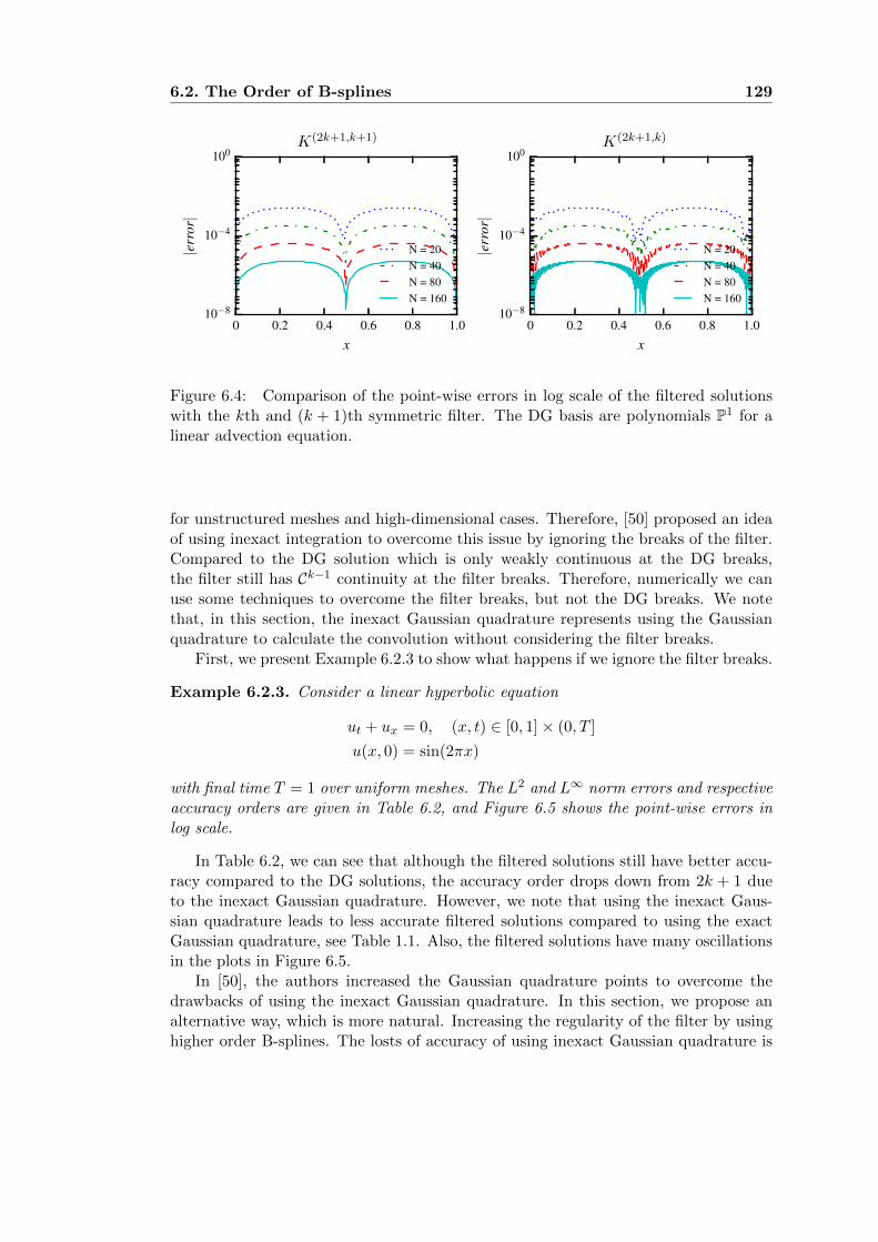
6.2. The Order of B-splines 129
K(2k+1,k+1) K(2k+1,k)
0 0.2 0.4 0.6 0.8 1.0
x
10−8
10−4
100
|erro
r|
N = 20N = 40N = 80N = 160
0 0.2 0.4 0.6 0.8 1.0
x
10−8
10−4
100
|erro
r|
N = 20N = 40N = 80N = 160
Figure 6.4: Comparison of the point-wise errors in log scale of the filtered solutionswith the kth and (k + 1)th symmetric filter. The DG basis are polynomials P1 for alinear advection equation.
for unstructured meshes and high-dimensional cases. Therefore, [50] proposed an ideaof using inexact integration to overcome this issue by ignoring the breaks of the filter.Compared to the DG solution which is only weakly continuous at the DG breaks,the filter still has Ck−1 continuity at the filter breaks. Therefore, numerically we canuse some techniques to overcome the filter breaks, but not the DG breaks. We notethat, in this section, the inexact Gaussian quadrature represents using the Gaussianquadrature to calculate the convolution without considering the filter breaks.
First, we present Example 6.2.3 to show what happens if we ignore the filter breaks.
Example 6.2.3. Consider a linear hyperbolic equation
ut + ux = 0, (x, t) ∈ [0, 1]× (0, T ]
u(x, 0) = sin(2πx)
with final time T = 1 over uniform meshes. The L2 and L∞ norm errors and respectiveaccuracy orders are given in Table 6.2, and Figure 6.5 shows the point-wise errors inlog scale.
In Table 6.2, we can see that although the filtered solutions still have better accu-racy compared to the DG solutions, the accuracy order drops down from 2k + 1 dueto the inexact Gaussian quadrature. However, we note that using the inexact Gaus-sian quadrature leads to less accurate filtered solutions compared to using the exactGaussian quadrature, see Table 1.1. Also, the filtered solutions have many oscillationsin the plots in Figure 6.5.
In [50], the authors increased the Gaussian quadrature points to overcome thedrawbacks of using the inexact Gaussian quadrature. In this section, we propose analternative way, which is more natural. Increasing the regularity of the filter by usinghigher order B-splines. The losts of accuracy of using inexact Gaussian quadrature is
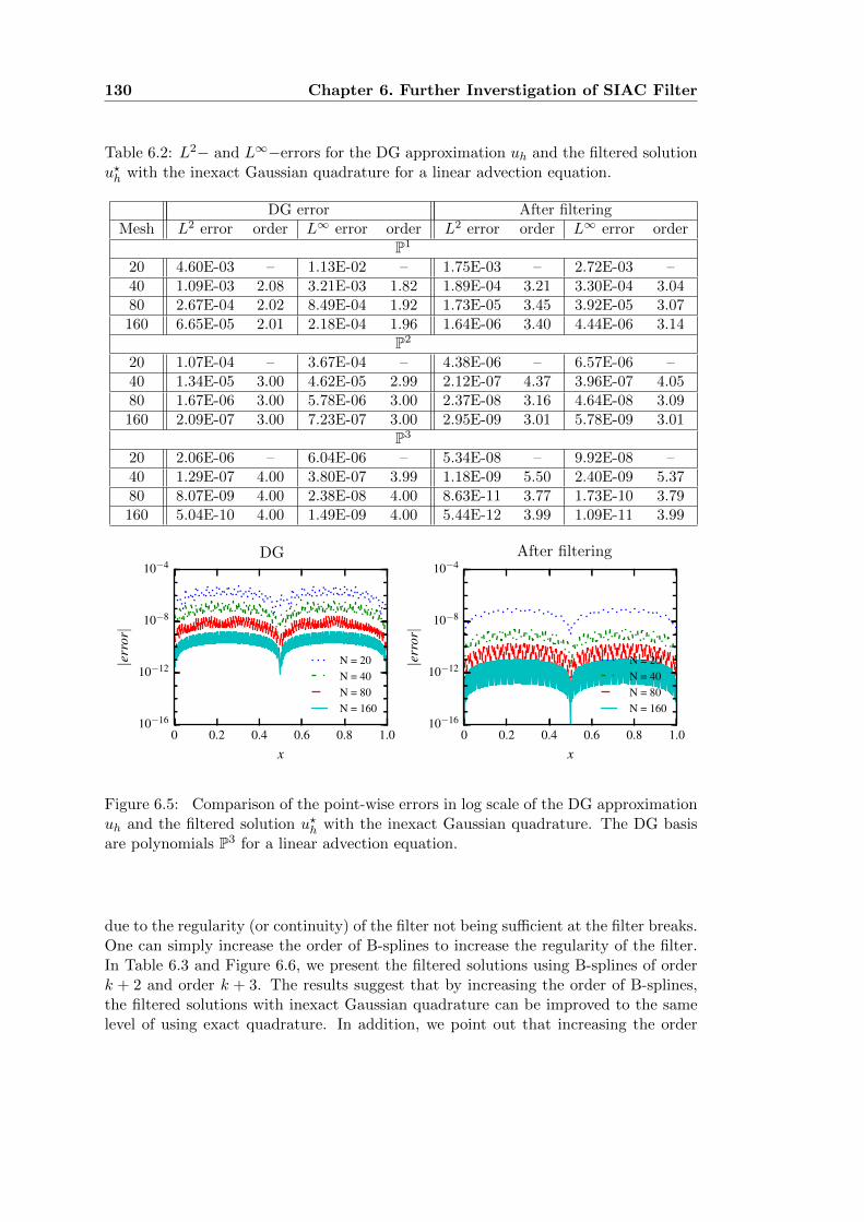
130 Chapter 6. Further Inverstigation of SIAC Filter
Table 6.2: L2− and L∞−errors for the DG approximation uh and the filtered solutionu?h with the inexact Gaussian quadrature for a linear advection equation.
DG error After filteringMesh L2 error order L∞ error order L2 error order L∞ error order
P1
20 4.60E-03 – 1.13E-02 – 1.75E-03 – 2.72E-03 –40 1.09E-03 2.08 3.21E-03 1.82 1.89E-04 3.21 3.30E-04 3.0480 2.67E-04 2.02 8.49E-04 1.92 1.73E-05 3.45 3.92E-05 3.07160 6.65E-05 2.01 2.18E-04 1.96 1.64E-06 3.40 4.44E-06 3.14
P2
20 1.07E-04 – 3.67E-04 – 4.38E-06 – 6.57E-06 –40 1.34E-05 3.00 4.62E-05 2.99 2.12E-07 4.37 3.96E-07 4.0580 1.67E-06 3.00 5.78E-06 3.00 2.37E-08 3.16 4.64E-08 3.09160 2.09E-07 3.00 7.23E-07 3.00 2.95E-09 3.01 5.78E-09 3.01
P3
20 2.06E-06 – 6.04E-06 – 5.34E-08 – 9.92E-08 –40 1.29E-07 4.00 3.80E-07 3.99 1.18E-09 5.50 2.40E-09 5.3780 8.07E-09 4.00 2.38E-08 4.00 8.63E-11 3.77 1.73E-10 3.79160 5.04E-10 4.00 1.49E-09 4.00 5.44E-12 3.99 1.09E-11 3.99
DG After filtering
0 0.2 0.4 0.6 0.8 1.0
x
10−16
10−12
10−8
10−4
|erro
r|
N = 20N = 40N = 80N = 160
0 0.2 0.4 0.6 0.8 1.0
x
10−16
10−12
10−8
10−4
|erro
r|
N = 20N = 40N = 80N = 160
Figure 6.5: Comparison of the point-wise errors in log scale of the DG approximationuh and the filtered solution u?h with the inexact Gaussian quadrature. The DG basisare polynomials P3 for a linear advection equation.
due to the regularity (or continuity) of the filter not being sufficient at the filter breaks.One can simply increase the order of B-splines to increase the regularity of the filter.In Table 6.3 and Figure 6.6, we present the filtered solutions using B-splines of orderk + 2 and order k + 3. The results suggest that by increasing the order of B-splines,the filtered solutions with inexact Gaussian quadrature can be improved to the samelevel of using exact quadrature. In addition, we point out that increasing the order

6.2. The Order of B-splines 131
of B-splines also slightly increases the support size of the filter. However, the extracost of the increased support size is negligible compare to using the exact Gaussianquadrature.
Table 6.3: L2− and L∞−errors for the filtered solution u?h with the inexact Gaus-sian quadrature for a linear advection equation. The filters used are K(2k+1,k+2) andK(2k+1,k+3).
K(2k+1,k+2) K(2k+1,k+3)
Mesh L2 error order L∞ error order L2 error order L∞ error orderP1
20 2.03E-03 – 2.87E-03 – 2.09E-03 – 2.96E-03 –40 2.47E-04 3.04 3.50E-04 3.04 2.51E-04 3.06 3.56E-04 3.0680 3.05E-05 3.02 4.31E-05 3.02 3.07E-05 3.03 4.35E-05 3.03160 3.78E-06 3.01 5.34E-06 3.01 3.80E-06 3.02 5.37E-06 3.02
P2
20 5.47E-06 – 7.76E-06 – 7.26E-06 – 1.03E-05 –40 1.16E-07 5.56 1.65E-07 5.55 1.45E-07 5.64 2.05E-07 5.6480 2.76E-09 5.39 4.01E-09 5.37 3.28E-09 5.47 4.64E-09 5.47160 7.85E-11 5.14 1.17E-10 5.09 8.99E-11 5.19 1.27E-10 5.19
P3
20 1.08E-07 – 1.53E-07 – 1.59E-07 – 2.25E-07 –40 4.38E-10 7.95 6.20E-10 7.95 6.44E-10 7.95 9.10E-10 7.9580 1.85E-12 7.89 2.63E-12 7.88 2.65E-12 7.93 3.74E-12 7.93160 1.93E-14 6.58 2.89E-14 6.51 2.14E-14 6.95 3.03E-14 6.95
K(2k+1,k+2) K(2k+1,k+3)
0 0.2 0.4 0.6 0.8 1.0
x
10−16
10−12
10−8
10−4
|erro
r|
N = 20N = 40N = 80N = 160
0 0.2 0.4 0.6 0.8 1.0
x
10−16
10−12
10−8
10−4
|erro
r|
N = 20N = 40N = 80N = 160
Figure 6.6: Comparison of the point-wise errors in log scale of the filtered solu-tions with the inexact Gaussian quadrature. The filters used are K(2k+1,k+2) andK(2k+1,k+3). The DG basis are polynomials P3 for a linear advection equation.
The idea of the inexact Gaussian quadrature is intended to reduce the compu-

132 Chapter 6. Further Inverstigation of SIAC Filter
tational cost of using SIAC filters. The benefits are not obvious for one-dimensionaluniform mesh cases. However, this idea has great potential value for multi-dimensionalapplications especially for unstructured meshes. For example, consider the two dimen-sional unstructured triangular meshes, it is computationally expensive to divide theintegration region into subregions, and numerical quadrature over these irregular sub-regions is also very expensive. The computational costs will become more expensivein three-dimensional cases, such as tetrahedral meshes. This is the reason a methodthat allows us to ignore the filter breaks has great potential values with respect to thecomputational considerations, and it is a subject of future work.
6.3 SIAC Filtering for Wave Functions
Wave functions are used in many branches of mathematics, science and engineer-ing. Mathematically, wave propagation problems are usually described by hyperbolicequations, and developing efficient methods and algorithms to solve wave-related ap-plication problems becomes an interesting task. In this section, we will introducethe preliminary methods of using SIAC filters to enhance the discontinuous Galerkinsolutions that relate to wave functions.
6.3.1 Sufficient Elements of the DG Approximation
It is well known that when using piecewise polynomials to approximate a wave function,one should at least use a certain number elements-per-wavelength. In other words,in order to approximate a wave function, we need sufficient resolution for the DGapproximation.
Consider a simple example, a sine function with λ wavenumber in the domain [0, 1],sin(2λπx). First we expand sin(2λπx) into Legendre polynomials. Denote ξ = 2x− 1,then we have
sin(2λπx) = sin(λπ(ξ + 1)), ξ ∈ [−1, 1].The Legendre expansion can be written as
sin(λπ(ξ + 1)) =∞∑n=0
anPn(ξ),
where Pn is the Legendre polynomials of degree n over [−1, 1] and
an =1√2λ
(2n+ 1)Jn+1/2(λπ) sin(λπ + nπ/2).
Here, Jn+1/2 is the Bessel function of the first kind of order n + 1/2. If the approxi-mation is given as a polynomial of degree k, then the truncation error E(λ, k) is
|E(λ, k)| ≤∞∑
n=k+1
|an|.
Here, the coefficient an satisfies
|an| ≤1√2λ
(2n+ 1)|Jn+1/2(λπ)|.
6.3. SIAC Filtering for Wave Functions 133
If N elements are used for the approximation, which means the wavenumber on eachelement is λ/N , then the new error is
|E(λ, k,N)| ≤∞∑
n=k+1
1√2λ/N
(2n+ 1)
∣∣∣∣Jn+1/2
(λπ
N
)∣∣∣∣ .Using the asymptotic form for the Bessel function (as x→ 0) (Eq. (9.1.7) in [1])
Jv(x) ∼1
Γ(v + 1)
(x2
)v,
we have
|an| ≤1√2λ/N
(2n+ 1)
(λπ
2N
)n+1/2 1
Γ(n+ 3/2)
=1√2λ/N
(2n+ 1)
(λπ
2N
)n+1/2 4n+1(n+ 1)!√π(2n+ 2)!
=1
(2n− 1)!!
(λπ
N
)n
Since h = 2N , we obtain the lowest order term of h for the truncation error,
|E(λ, k,N)| ≤ (λπ)k+1
(2k + 1)!!hk+1.
The required number of elements, N λπ, is needed for this desired accuracy.Then, we check the details of the condition N λπ. This condition is required by
using the asymptotic form for the Bessel function of the first kind that
Jv(z) ∼ (1
2z)v/Γ(v + 1).
The above asymptotic form requires z → 0 when v is fixed. In the above error esti-mate, z = λπ
N , then we get N λπ. In order to understand further details of thisrequirement, we write the exact formula of the Bessel function of the first kind (Eq(9.1.10) in [1]),
Jv(z) =(z2
)v ∞∑n=0
bn(z) =(z2
)v ∞∑n=0
(− z2
4
)nn!Γ(v + n+ 1)
.
Comparing the first term b0(z) and the second b1(z) with z =λπN and v = k + 3/2,
|b0(z)/b1(z)| =4Γ(v + 2)
z2Γ(v + 1)=
4(v + 1)
z2=
(4k + 6)N2
(λπ)2.
Therefore, we can require b0(z)/b1(z) ≥ N to guarantee a reasonable accuracy andaccuracy order. This means,
(4k + 6)N2
(λπ)2≥ N =⇒ N ≥ (λπ)2
4k + 6.
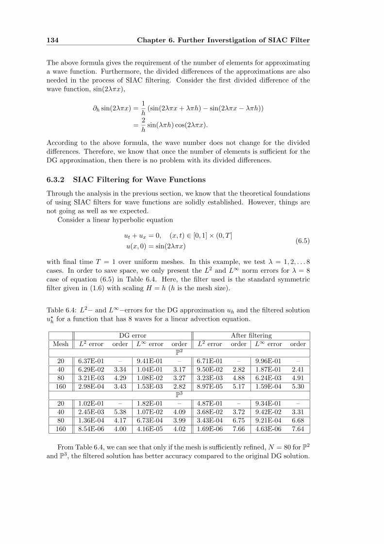
134 Chapter 6. Further Inverstigation of SIAC Filter
The above formula gives the requirement of the number of elements for approximatinga wave function. Furthermore, the divided differences of the approximations are alsoneeded in the process of SIAC filtering. Consider the first divided difference of thewave function, sin(2λπx),
∂h sin(2λπx) =1
h(sin(2λπx+ λπh)− sin(2λπx− λπh))
=2
hsin(λπh) cos(2λπx).
According to the above formula, the wave number does not change for the divideddifferences. Therefore, we know that once the number of elements is sufficient for theDG approximation, then there is no problem with its divided differences.
6.3.2 SIAC Filtering for Wave Functions
Through the analysis in the previous section, we know that the theoretical foundationsof using SIAC filters for wave functions are solidly established. However, things arenot going as well as we expected.
Consider a linear hyperbolic equation
ut + ux = 0, (x, t) ∈ [0, 1]× (0, T ]
u(x, 0) = sin(2λπx)(6.5)
with final time T = 1 over uniform meshes. In this example, we test λ = 1, 2, . . . 8cases. In order to save space, we only present the L2 and L∞ norm errors for λ = 8case of equation (6.5) in Table 6.4. Here, the filter used is the standard symmetricfilter given in (1.6) with scaling H = h (h is the mesh size).
Table 6.4: L2− and L∞−errors for the DG approximation uh and the filtered solutionu?h for a function that has 8 waves for a linear advection equation.
DG error After filteringMesh L2 error order L∞ error order L2 error order L∞ error order
P2
20 6.37E-01 – 9.41E-01 – 6.71E-01 – 9.96E-01 –40 6.29E-02 3.34 1.04E-01 3.17 9.50E-02 2.82 1.87E-01 2.4180 3.21E-03 4.29 1.08E-02 3.27 3.23E-03 4.88 6.24E-03 4.91160 2.98E-04 3.43 1.53E-03 2.82 8.97E-05 5.17 1.59E-04 5.30
P3
20 1.02E-01 – 1.82E-01 – 4.87E-01 – 9.34E-01 –40 2.45E-03 5.38 1.07E-02 4.09 3.68E-02 3.72 9.42E-02 3.3180 1.36E-04 4.17 6.73E-04 3.99 3.43E-04 6.75 9.21E-04 6.68160 8.54E-06 4.00 4.16E-05 4.02 1.69E-06 7.66 4.63E-06 7.64
From Table 6.4, we can see that only if the mesh is sufficiently refined, N = 80 for P2
and P3, the filtered solution has better accuracy compared to the original DG solution.
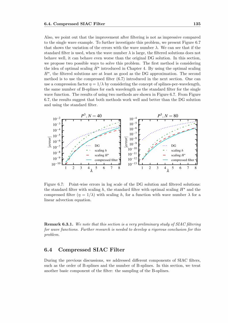
6.4. Compressed SIAC Filter 135
Also, we point out that the improvement after filtering is not as impressive comparedto the single wave example. To further investigate this problem, we present Figure 6.7that shows the variation of the errors with the wave number λ. We can see that if thestandard filter is used, when the wave number λ is large, the filtered solutions does notbehave well, it can behave even worse than the original DG solution. In this section,we propose two possible ways to solve this problem. The first method is consideringthe idea of optimal scaling H? introduced in Chapter 4. By using the optimal scalingH?, the filtered solutions are at least as good as the DG approximation. The secondmethod is to use the compressed filter (6.7) introduced in the next section. One canuse a compression factor η = 1/λ by considering the concept of splines-per-wavelength,the same number of B-splines for each wavelength as the standard filter for the singlewave function. The results of using two methods are shown in Figure 6.7. From Figure6.7, the results suggest that both methods work well and better than the DG solutionand using the standard filter.
1 2 3 4 5 6 7 8λ
10−1010−910−810−710−610−510−410−310−2
|erro
r|
P3, N = 40
DGscaling hscaling H?
compressed filter
1 2 3 4 5 6 7 8λ
10−1310−1210−1110−1010−910−810−710−610−510−4
|erro
r|
P3, N = 80
DGscaling hscaling H?
compressed filter
Figure 6.7: Point-wise errors in log scale of the DG solution and filtered solutions:the standard filter with scaling h, the standard filter with optimal scaling H? and thecompressed filter (η = 1/λ) with scaling h, for a function with wave number λ for alinear advection equation.
Remark 6.3.1. We note that this section is a very preliminary study of SIAC filteringfor wave functions. Further research is needed to develop a rigorous conclusion for thisproblem.
6.4 Compressed SIAC Filter
During the previous discussions, we addressed different components of SIAC filters,such as the order of B-splines and the number of B-splines. In this section, we treatanother basic component of the filter: the sampling of the B-splines.

136 Chapter 6. Further Inverstigation of SIAC Filter
Recall the formula of the symmetric filter,
K(2k+1,k+1)(x) =
r∑γ=0
c(2k+1,k+1)γ ψ(k+1)(x+ k − γ). (6.6)
In formula (6.6), the B-splines are uniformly distributed with distance 1. However,the proof of Theorem 1.3.4 suggests that the sampling of the 2k + 1 B-splines has noeffect on the final accuracy order, 2k + 1. The theoretical results allow us to samplein different ways. It is then important to sample the B-splines in a way that we canobtain additional benefits.
As mentioned earlier, one important computational factor of the filter is its supportsize. A large support size usually leads to many computational problems. Based onthis, we can sample the B-splines more closely to each other and reduce the supportsize of the filter.
K(2k+1,k+1)η (x) =
r∑γ=0
c(2k+1,k+1)γ ψ(k+1)(x− xγ), (6.7)
where the sampling isxγ = η(−k + γ).
Here, we refer to the filter given in (6.7) as the compressed filter and η as the com-pression factor. Figure 6.8 shows the compressed filters with η = 0.5, see the originalfilters in Figure 1.2. The support size of the compressed filter is (2η + 1)k + 1.
Remark 6.4.1. If one changes the scaling of the original filter in (6.6) by a scaling
H = (2η+1)k+13k+1 , then the scaled filter K
(2k+1,k+1)H has the same support size as the
compressed filter K(2k+1,k+1)η . However, these two filters are not equivalent. Only the
compressed filter is able to obtain supperconvergence.
k = 1
−2 −1 0 1 2−0.4
0.0
0.4
0.8
1.2
1.6k = 2
−3 −2 −1 0 1 2 3−0.4
0.0
0.4
0.8
1.2
1.6k = 3
−4 −3 −2 −1 0 1 2 3 4−0.4
0.0
0.4
0.8
1.2
1.6
Figure 6.8: Solid black lines represent the compressed filter K(2k+1,k+1)η given in
(6.7) with k = 1, 2, 3, dashed red lines represent the respect central B-splines. Thecompression factor η = 0.5.
For the filtered solutions, we denote the scaled compressed filter as K(2k+1,k)h,η (x) =
1hK
(2k+1,k+1)η , then one can prove

6.4. Compressed SIAC Filter 137
Theorem 6.4.1. Under the same conditions in Theorem 1.3.4, the compressed filterdefined in (6.7) with η > 0, then
‖u−K(2k+1,k)h,η ? uh‖0,Ω0 ≤ Ch2k+1.
Proof. The proof is the same as in Theorem 1.3.4.
Example 6.4.2. Consider a linear hyperbolic equation
ut + ux = 0, (x, t) ∈ [0, 1]× (0, T ]
u(x, 0) = sin(2πx)
with final time T = 1 over uniform meshes. The L2 and L∞ norm errors and respectiveaccuracy orders are given in Table 6.5. Figure 6.9 shows the point-wise errors in logscale. The respective results of the DG approximation and the original filtered solutioncan be found in Example 1.3.5.
Table 6.5: L2− and L∞−errors for the filtered solution u?h with compressed filters(η = 0.5 and η = 0.25) for a linear advection equation.
K(2k+1,k+1)0.5 K
(2k+1,k+1)0.25
Mesh L2 error order L∞ error order L2 error order L∞ error orderP1
20 1.94E-03 – 2.78E-03 – 1.93E-03 – 2.78E-03 –40 2.42E-04 3.00 3.44E-04 3.01 2.41E-04 3.00 3.44E-04 3.0180 3.01E-05 3.00 4.27E-05 3.01 3.01E-05 3.00 4.27E-05 3.01160 3.76E-06 3.00 5.32E-06 3.01 3.75E-06 3.00 5.32E-06 3.01
P2
20 2.51E-06 – 3.66E-06 – 2.27E-06 – 3.47E-06 –40 6.95E-08 5.17 1.00E-07 5.19 6.57E-08 5.11 9.72E-08 5.1680 2.09E-09 5.06 2.98E-09 5.07 2.03E-09 5.02 2.94E-09 5.05160 7.12E-11 4.87 1.01E-10 4.88 7.03E-11 4.85 1.01E-10 4.87
P3
20 1.11E-08 – 1.57E-08 – 5.89E-09 – 9.15E-09 –40 4.81E-11 7.84 6.86E-11 7.84 2.76E-11 7.74 4.25E-11 7.7580 3.04E-13 7.30 4.33E-13 7.31 2.24E-13 6.95 3.30E-13 7.01160 1.23E-14 4.63 1.74E-14 4.64 1.20E-14 4.23 1.70E-14 4.28
Through Example 6.4.2, we can see the compressed filter works as good as theoriginal filter, same accuracy order, same error level and same smoothness. The com-pressed filter has reduced support size and maintains the same accuracy level as theoriginal filter. The compressed filter idea can help solve many issues caused by the largesupport size of the filter, such as filtering over nonuniform meshes and boundaries. Itis a subject of future work.

138 Chapter 6. Further Inverstigation of SIAC Filter
K(2k+1,k+1)0.5 K
(2k+1,k+1)0.25
0 0.2 0.4 0.6 0.8 1.0
x
10−16
10−12
10−8
10−4
|erro
r|
N = 20N = 40N = 80N = 160
0 0.2 0.4 0.6 0.8 1.0
x
10−16
10−12
10−8
10−4
|erro
r|
N = 20N = 40N = 80N = 160
Figure 6.9: Point-wise errors in log scale of the filtered solutions with compressedfilters (η = 0.5 and η = 0.25). The DG basis are polynomials P3 for a linear advectionequation.
6.5 Conclusion
In this chapter, we have discussed several interesting topics of SIAC filters. Each topiccan lead us to a deeper understanding of SIAC filters and can be further studied. Here,we just name a few future problems that are based on the topics in this chapter:
• Fast SIAC filtering for unstructured meshes and high-dimensional problems bycombining the idea of the inexact Gaussian quadrature and the compressed filter.
• SIAC filtering for wave-related application problems by using the compressedfilter or the optimal scaling concept.
• New structured filters based on Section 6.1, such as infinity smooth filter, trigono-metric filter, etc.

7Conclusion and Future Work
In this dissertation, we focus on exploiting superconvergence for discontinuous Galerkinsolutions and constructing a superconvergence extraction techniques, in particular,Smoothness-Increasing Accuracy-Conserving filtering. We contributed to a series ofstudies of SIAC filters for a variety of circumstances by proving theoretical analysis andnumerical experiments. The particular contributions of this thesis are the following:
• One-Sided SIAC Filtering Over Uniform and Nonuniform Meshes.Typically, most of the studies of SIAC filtering are confined to the interior of theunderlying domain. For boundary regions, a one-sided filter is needed. The exist-ing one-sided filters are not directly useful for most applications since they werelimited to uniform meshes, linear equations, using multi-precision pages in com-putation. Also, the theoretical proof relied on a periodic boundary assumption.We aimed to overcome these deficiencies and develop a new fast one-sided filterfor both uniform and nonuniform meshes. By studying B-splines and the negativeorder norm analysis, we generalized the structure of SIAC filters from a combi-nation of central B-splines to using more general B-splines. Then, a “boundaryshape” B-spline (using multiplicity knots at the boundary) was used to constructa new one-sided filter. We also presented the first theoretical proof of convergencefor SIAC filtering over nonuniform meshes (smoothly-varying meshes). Detailsare given in Chapter 2.
• Derivative Filtering Over Nonuniform Meshes and Near Boundaries.One advantage of SIAC filtering is that it improves the smoothness of DG solu-tions. Because of the increased smoothness, we can obtain a better approxima-tion of the derivatives of DG solutions. The derivative filtering over the interiorregion of uniform meshes was previously studied. However, nonuniform meshesand boundary regions still remain a big challenge. We extended the one-sidedfilter to a one-sided derivative filter. Nonuniform meshes are a difficult area,by investigating the negative order norm over arbitrary meshes, we proposed toscale the one-sided derivative filter with scaling hµ. For arbitrary nonuniformrectangle meshes, we proved that the one-sided derivative filter can enhance theorder of convergence for αth derivative of DG solution from k+1−α to µ(2k+2),
139

140 Chapter 7. Conclusion and Future Work
where µ ≈ 23 . Details are in Chapter 3.
• Superconvergence Extraction Over Nonuniform Meshes. The most chal-lenging part of this project is recovering the superconvergence of a DG solu-tion over nonuniform meshes through SIAC filtering. Typically, most theoreticalproofs for the SIAC filter are limited to uniform meshes (or translation invariantmeshes). The few theoretical investigations for nonuniform meshes were givenin the one-sided and derivative filtering studies. Although our early research fornonuniform meshes was able to provide good engineering accuracy, we want todo better mathematically. This is not an easy task since unstructured meshesgive DG solutions irregular performance under the negative order norm. In ourwork, we introduced a parameter to measure the “unstructuredness” of a givennonuniform mesh. Then by adjusting the scaling of SIAC filter based on this“unstructuredness” parameter, we are able to obtain the optimal filtered approx-imation (best accuracy) over a given nonuniform mesh. Details are in Chapter4.
• Application to Streamline Integration. After introducing the new one-sidedfilter, we aimed to verify its usage in realistic engineering applications. Thetopic we chose was streamline integration. By taking advantage of the one-sidedproperty of the new filter, we designed an efficient algorithm which filters thevelocity field along the streamline, then uses a backward differentiation formula(BDF) for integration. Compared to the traditional method that filters the entirefield (multi-dimensions algorithm), the computational cost drops dramaticallysince it is only a one-dimensional algorithm. Details can be found in Chapter 5.
• Further Topics of SIAC Filters. After studying SIAC filters for a broad rangeof applications, we returned to further investigations of SIAC filters themselves.Further topics such the uniqueness of the structure SIAC filters, the effects of theorder of B-splines to SIAC filters and the compressed SIAC filters are includedin Chapter 6. These topics give us in-depth insight into SIAC filters and revealsome future directions for the development of SIAC filters.
Future Work
• This dissertation studies the superconvergence and SIAC filters for DG methods.The extension is also possible to other numerical methods, such as finite elementmethods, finite volume methods, finite difference methods and spectral methods.
• The theoretical error estimates for SIAC filters are only established for linearhyperbolic problems. Nevertheless, the numerical results suggest that the filterswork well for a broad range of problems, such as variable coefficient equationsand linear hyperbolic conservation laws. Theoretical support for the nonlinearproblems could be a significant step towards real-world applications.
• Uniform or nonuniform quadrilateral meshes were considered in this disserta-tion. The extension of SIAC filters for unstructured triangular or tetrahedraltessellation is still a problem that is not perfectly solved. Developing an efficient

141
and accurate way to use SIAC filters over these unstructured meshes has greatpractical values.
• The mathematical foundation of SIAC filters has been well established for manysituations. It is time to evolve SIAC filters widely to real-world applications. Forexample, the use of SIAC filters for streamline integration is a subject of ongoingresearch.

Bibliography
[1] Milton Abramowitz and Irene A. Stegun, editors. Handbook of mathemat-ical functions with formulas, graphs, and mathematical tables. Dover Pub-lications, Inc., New York, 1992. Reprint of the 1972 edition. http://peo-ple.math.sfu.ca/∼cbm/aands/intro.htm.
[2] Slimane Adjerid and Mahboub Baccouch. The discontinuous Galerkin method fortwo-dimensional hyperbolic problems. II. A posteriori error estimation. J. Sci.Comput., 38(1):15–49, 2009.
[3] Slimane Adjerid and Mahboub Baccouch. A superconvergent local discontinuousGalerkin method for elliptic problems. J. Sci. Comput., 52(1):113–152, 2012.
[4] Slimane Adjerid, Karen D. Devine, Joseph E. Flaherty, and Lilia Krivodonova.A posteriori error estimation for discontinuous Galerkin solutions of hyperbolicproblems. Comput. Methods Appl. Mech. Engrg., 191(11-12):1097–1112, 2002.
[5] Slimane Adjerid and Idir Mechai. A superconvergent discontinuous Galerkinmethod for hyperbolic problems on tetrahedral meshes. J. Sci. Comput.,58(1):203–248, 2014.
[6] Slimane Adjerid and Helmi Temimi. A discontinuous Galerkin method for thewave equation. Comput. Methods Appl. Mech. Engrg., 200(5-8):837–849, 2011.
[7] Rick Archibald, Anne Gelb, Sigal Gottlieb, and Jennifer K. Ryan. One-sidedpost-processing for the discontinuous Galerkin method using ENO type stencilchoosing and the local edge detection method. J. Sci. Comput., 28(2-3):167–190,2006.
[8] Mahboub Baccouch. The local discontinuous Galerkin method for the fourth-order Euler-Bernoulli partial differential equation in one space dimension. Part I:Superconvergence error analysis. J. Sci. Comput., 59(3):795–840, 2014.
143

144 BIBLIOGRAPHY
[9] Mahboub Baccouch. The local discontinuous Galerkin method for the fourth-orderEuler-Bernoulli partial differential equation in one space dimension. Part II: Aposteriori error estimation. J. Sci. Comput., 60(1):1–34, 2014.
[10] Mahboub Baccouch. Superconvergence and a posteriori error estimates of a localdiscontinuous Galerkin method for the fourth-order initial-boundary value prob-lems arising in beam theory. Int. J. Numer. Anal. Model. Ser. B, 5(3):188–216,2014.
[11] Mahboub Baccouch and Slimane Adjerid. Discontinuous Galerkin error estimationfor hyperbolic problems on unstructured triangular meshes. Comput. MethodsAppl. Mech. Engrg., 200(1-4):162–177, 2011.
[12] Georges-Pierre Bonneau, Thomas Ertl, and Gregory M. Nielson, editors. Scientificvisualization: the visual extraction of knowledge from data. Mathematics andVisualization. Springer-Verlag, Berlin, 2006.
[13] J. H. Bramble and A. H. Schatz. Higher order local accuracy by averaging in thefinite element method. Math. Comp., 31(137):94–111, 1977.
[14] Susanne C. Brenner and L. Ridgway Scott. The mathematical theory of finiteelement methods, volume 15 of Texts in Applied Mathematics. Springer, NewYork, third edition, 2008.
[15] Waixiang Cao, Zhimin Zhang, and Qingsong Zou. Superconvergence of discontin-uous Galerkin methods for linear hyperbolic equations. SIAM J. Numer. Anal.,52(5):2555–2573, 2014.
[16] Fatih Celiker and Bernardo Cockburn. Element-by-element post-processingof discontinuous Galerkin methods for Timoshenko beams. J. Sci. Comput.,27(1-3):177–187, 2006.
[17] Yingda Cheng and Chi-Wang Shu. Superconvergence and time evolution of discon-tinuous Galerkin finite element solutions. J. Comput. Phys., 227(22):9612–9627,2008.
[18] Yingda Cheng and Chi-Wang Shu. Superconvergence of discontinuousGalerkin and local discontinuous Galerkin schemes for linear hyperbolic andconvection-diffusion equations in one space dimension. SIAM J. Numer. Anal.,47(6):4044–4072, 2010.
[19] Philippe G. Ciarlet. The finite element method for elliptic problems, volume 40 ofClassics in Applied Mathematics. Society for Industrial and Applied Mathematics(SIAM), Philadelphia, PA, 2002. Reprint of the 1978 original [North-Holland,Amsterdam; MR0520174 (58 #25001)].
[20] Bernardo Cockburn. An introduction to the discontinuous Galerkin method forconvection-dominated problems. In Advanced numerical approximation of nonlin-ear hyperbolic equations (Cetraro, 1997), volume 1697 of Lecture Notes in Math.,pages 151–268. Springer, Berlin, 1998.

BIBLIOGRAPHY 145
[21] Bernardo Cockburn. Discontinuous Galerkin methods for convection-dominatedproblems. In High-order methods for computational physics, volume 9 of Lect.Notes Comput. Sci. Eng., pages 69–224. Springer, Berlin, 1999.
[22] Bernardo Cockburn. Discontinuous Galerkin methods. ZAMM Z. Angew. Math.Mech., 83(11):731–754, 2003.
[23] Bernardo Cockburn, George E. Karniadakis, and Chi-Wang Shu, editors. Discon-tinuous Galerkin methods, volume 11 of Lecture Notes in Computational Scienceand Engineering. Springer-Verlag, Berlin, 2000. Theory, computation and appli-cations, Papers from the 1st International Symposium held in Newport, RI, May24–26, 1999.
[24] Bernardo Cockburn, George E Karniadakis, and Chi-Wang Shu. The developmentof discontinuous Galerkin methods. In Discontinuous Galerkin methods (Newport,RI, 1999), pages 3–50. Springer, Berlin, 2000.
[25] Bernardo Cockburn, Mitchell Luskin, Chi-Wang Shu, and Endre Suli. Enhancedaccuracy by post-processing for finite element methods for hyperbolic equations.Math. Comp., 72(242):577–606, 2003.
[26] Bernardo Cockburn and Chi-Wang Shu. TVB Runge-Kutta local projectiondiscontinuous Galerkin finite element method for conservation laws. II. Generalframework. Math. Comp., 52(186):411–435, 1989.
[27] Bernardo Cockburn and Chi-Wang Shu. The local discontinuous Galerkinmethod for time-dependent convection-diffusion systems. SIAM J. Numer. Anal.,35(6):2440–2463 (electronic), 1998.
[28] Bernardo Cockburn and Chi-Wang Shu. The Runge-Kutta discontinuous Galerkinmethod for conservation laws. V. Multidimensional systems. J. Comput. Phys.,141(2):199–224, 1998.
[29] Bernardo Cockburn and Chi-Wang Shu. Runge-Kutta discontinuous Galerkinmethods for convection-dominated problems. J. Sci. Comput., 16(3):173–261,2001.
[30] Sean Curtis, Robert M. Kirby, Jennifer K. Ryan, and Chi-Wang Shu. Postpro-cessing for the discontinuous Galerkin method over nonuniform meshes. SIAM J.Sci. Comput., 30(1):272–289, 2007/08.
[31] Carl de Boor. A practical guide to splines, volume 27 of Applied MathematicalSciences. Springer-Verlag, New York, revised edition, 2001.
[32] Daniele Antonio Di Pietro and Alexandre Ern. Mathematical aspects of discon-tinuous Galerkin methods, volume 69 of Mathematiques & Applications (Berlin)[Mathematics & Applications]. Springer, Heidelberg, 2012.
[33] Jim Douglas, Jr. and Todd Dupont. Some superconvergence results for Galerkinmethods for the approximate solution of two-point boundary problems. In Topics

146 BIBLIOGRAPHY
in numerical analysis (Proc. Roy. Irish Acad. Conf., University Coll., Dublin,1972), pages 89–92. Academic Press, London, 1973.
[34] Jim Douglas, Jr., Todd Dupont, and Mary Fanett Wheeler. Some superconver-gence results for an H1-Galerkin procedure for the heat equation. In Computingmethods in applied sciences and engineering (Proc. Internat. Sympos., Versailles,1973), Part 1, pages 288–311. Lecture Notes in Comput. Sci., Vol. 10. Springer,Berlin, 1974.
[35] Lawrence C. Evans. Partial differential equations, volume 19 of Graduate Studiesin Mathematics. American Mathematical Society, Providence, RI, 1998.
[36] Xiaobing Feng, Ohannes Karakashian, and Yulong Xing, editors. Recent devel-opments in discontinuous Galerkin finite element methods for partial differentialequations, volume 157 of The IMA Volumes in Mathematics and its Applications.Springer, Cham, 2014. 2012 John H. Barrett Memorial Lectures, Selected papersfrom the workshop held at the University of Tennessee, Knoxville, TN, May 9–11,2012.
[37] Casey Hufford and Yulong Xing. Superconvergence of the local discontinuousGalerkin method for the linearized Korteweg-de Vries equation. J. Comput. Appl.Math., 255:441–455, 2014.
[38] Arieh Iserles. A first course in the numerical analysis of differential equations.Cambridge Texts in Applied Mathematics. Cambridge University Press, Cam-bridge, second edition, 2009.
[39] Liangyue Ji, Paulien van Slingerland, Jennifer K. Ryan, and Kees Vuik. Supercon-vergent error estimates for position-dependent smoothness-increasing accuracy-conserving (SIAC) post-processing of discontinuous Galerkin solutions. Math.Comp., 83(289):2239–2262, 2014.
[40] Liangyue Ji, Yan Xu, and Jennifer K. Ryan. Accuracy-enhancement of discontin-uous Galerkin solutions for convection-diffusion equations in multiple-dimensions.Math. Comp., 81(280):1929–1950, 2012.
[41] Liangyue Ji, Yan Xu, and Jennifer K. Ryan. Negative-order norm estimates fornonlinear hyperbolic conservation laws. J. Sci. Comput., 54(2-3):531–548, 2013.
[42] C. Johnson and J. Pitkaranta. An analysis of the discontinuous Galerkin methodfor a scalar hyperbolic equation. Math. Comp., 46(173):1–26, 1986.
[43] James King, Hanieh Mirzaee, Jennifer K. Ryan, and Robert M. Kirby.Smoothness-increasing accuracy-conserving (SIAC) filtering for discontinuousGalerkin solutions: improved errors versus higher-order accuracy. J. Sci. Comput.,53(1):129–149, 2012.
[44] Michal Krızek and Pekka Neittaanmaki. Bibliography on superconvergence. InFinite element methods (Jyvaskyla, 1997), volume 196 of Lecture Notes in Pureand Appl. Math., pages 315–348. Dekker, New York, 1998.

BIBLIOGRAPHY 147
[45] P. Lasaint and P.-A. Raviart. On a finite element method for solving the neu-tron transport equation. In Mathematical aspects of finite elements in partialdifferential equations (Proc. Sympos., Math. Res. Center, Univ. Wisconsin, Madi-son, Wis., 1974), pages 89–123. Publication No. 33. Math. Res. Center, Univ. ofWisconsin-Madison, Academic Press, New York, 1974.
[46] Randall J. LeVeque. Finite volume methods for hyperbolic problems. CambridgeTexts in Applied Mathematics. Cambridge University Press, Cambridge, 2002.
[47] Xiaozhou Li, Yan Xu, and Yishen Li. Investigation of multi-soliton, multi-cusponsolutions to the Camassa-Holm equation and their interaction. Chin. Ann. Math.Ser. B, 33(2):225–246, 2012.
[48] Hanieh Mirzaee, James King, Jennifer K. Ryan, and Robert M. Kirby.Smoothness-increasing accuracy-conserving filters for discontinuous Galerkinsolutions over unstructured triangular meshes. SIAM J. Sci. Comput.,35(1):A212–A230, 2013.
[49] Hanieh Mirzaee, Jennifer K. Ryan, and Robert M. Kirby. Quantification of errorsintroduced in the numerical approximation and implementation of smoothness-increasing accuracy conserving (SIAC) filtering of discontinuous Galerkin (DG)fields. J. Sci. Comput., 45(1-3):447–470, 2010.
[50] Hanieh Mirzaee, Jennifer K. Ryan, and Robert M. Kirby. Efficient implementa-tion of smoothness-increasing accuracy-conserving (SIAC) filters for discontinuousGalerkin solutions. J. Sci. Comput., 52(1):85–112, 2012.
[51] Michael S. Mock and Peter D. Lax. The computation of discontinuous solutionsof linear hyperbolic equations. Comm. Pure Appl. Math., 31(4):423–430, 1978.
[52] Kassem Mustapha and Jennifer K. Ryan. Post-processing discontinuous Galerkinsolutions to Volterra integro-differential equations: analysis and simulations. J.Comput. Appl. Math., 253:89–103, 2013.
[53] Todd E. Peterson. A note on the convergence of the discontinuous Galerkinmethod for a scalar hyperbolic equation. SIAM J. Numer. Anal., 28(1):133–140,1991.
[54] W.H. Reed and T.R. Hill. Triangular mesh methods for the neutron transportequation. Los Alamos Report LA-UR-73-479, 1973.
[55] Jennifer K. Ryan. Local Derivative Post-processing: Challenges for a non-uniformmesh. Delft University of Technology Report 10-18, 2013.
[56] Jennifer K. Ryan and Bernardo Cockburn. Local derivative post-processing forthe discontinuous Galerkin method. J. Comput. Phys., 228(23):8642–8664, 2009.
[57] Jennifer K. Ryan and Chi-Wang Shu. On a one-sided post-processing techniquefor the discontinuous Galerkin methods. Methods Appl. Anal., 10(2):295–307,2003.

148 BIBLIOGRAPHY
[58] Jennifer K. Ryan, Chi-Wang Shu, and Harold Atkins. Extension of a postprocess-ing technique for the discontinuous Galerkin method for hyperbolic equations withapplication to an aeroacoustic problem. SIAM J. Sci. Comput., 26(3):821–843,2005.
[59] Alfred H. Schatz. Pointwise error estimates and asymptotic error expansion in-equalities for the finite element method on irregular grids. I. Global estimates.Math. Comp., 67(223):877–899, 1998.
[60] Larry L. Schumaker. Spline functions: basic theory. Cambridge MathematicalLibrary. Cambridge University Press, Cambridge, third edition, 2007.
[61] M Steffen, S Curtis, R M Kirby, and J K Ryan. Investigation of Smoothness-Increasing Accuracy-Conserving Filters for Improving Streamline IntegrationThrough Discontinuous Fields. Visualization and Computer Graphics, IEEETransactions on, 14(3):680–692, 2008.
[62] Vidar Thomee. High order local approximations to derivatives in the finite elementmethod. Math. Comp., 31(139):652–660, 1977.
[63] Vidar Thomee. Negative norm estimates and superconvergence in Galerkin meth-ods for parabolic problems. Math. Comp., 34(149):93–113, 1980.
[64] Paulien van Slingerland, Jennifer K. Ryan, and C Vuik. Smoothness-IncreasingConvergence-Conserving Spline Filters Applied to Streamline Visualization ofDG Approximations. Delft University of Technology Report 09-06, 2009.http://ta.twi.tudelft.nl/nw/users/vuik/papers/Sli09RV.pdf.
[65] Paulien van Slingerland, Jennifer K. Ryan, and C. Vuik. Position-dependentsmoothness-increasing accuracy-conserving (SIAC) filtering for improving discon-tinuous Galerkin solutions. SIAM J. Sci. Comput., 33(2):802–825, 2011.
[66] M.J. Vuik. Limiting and shock detection for discontinuous Galerkin solutions usingmultiwavelet. TU Delft MSc Thesis, 2012. http://ta.twi.tudelft.nl/users/vuik/nu-manal/vuik afst.pdf.
[67] Lars B. Wahlbin. Superconvergence in Galerkin finite element methods, volume1605 of Lecture Notes in Mathematics. Springer-Verlag, Berlin, 1995.
[68] David Walfisch, Jennifer K. Ryan, Robert M. Kirby, and Robert Haimes. One-sided smoothness-increasing accuracy-conserving filtering for enhanced streamlineintegration through discontinuous fields. J. Sci. Comput., 38(2):164–184, 2009.
[69] Ziqing Xie and Zhimin Zhang. Uniform superconvergence analysis of the discon-tinuous Galerkin method for a singularly perturbed problem in 1-D. Math. Comp.,79(269):35–45, 2010.
[70] Yan Xu and Chi-wang Shu. Local discontinuous Galerkin methods for three classesof nonlinear wave equations. J. Comput. Math., 22(2):250–274, 2004. Special issuededicated to the 70th birthday of Professor Zhong-Ci Shi.

BIBLIOGRAPHY 149
[71] Yan Xu and Chi-Wang Shu. Local discontinuous Galerkin methods for nonlinearSchrodinger equations. J. Comput. Phys., 205(1):72–97, 2005.
[72] Yan Xu and Chi-Wang Shu. Local discontinuous Galerkin methods for theKuramoto-Sivashinsky equations and the Ito-type coupled KdV equations. Com-put. Methods Appl. Mech. Engrg., 195(25-28):3430–3447, 2006.
[73] Yan Xu and Chi-Wang Shu. A local discontinuous Galerkin method for theCamassa-Holm equation. SIAM J. Numer. Anal., 46(4):1998–2021, 2008.
[74] Yang Yang and Chi-Wang Shu. Analysis of optimal superconvergence of discon-tinuous Galerkin method for linear hyperbolic equations. SIAM J. Numer. Anal.,50(6):3110–3133, 2012.
[75] Yang Yang and Chi-Wang Shu. Discontinuous Galerkin method for hyperbolicequations involving δ-singularities: negative-order norm error estimates and ap-plications. Numer. Math., 124(4):753–781, 2013.
[76] Tie Zhang and Shun Yu. The derivative patch interpolation recovery techniqueand superconvergence for the discontinuous Galerkin method. Appl. Numer.Math., 85:128–141, 2014.
[77] Zuozheng Zhang, Ziqing Xie, and Zhimin Zhang. Superconvergence of discon-tinuous Galerkin methods for convection-diffusion problems. J. Sci. Comput.,41(1):70–93, 2009.

Curriculum vitae
Xiaozhou Li
• 2010.12 - 2015.7: Ph.D., Delft Institute of Applied Mathematics, Delft Universityof Technology, The Netherlands.
– Supervisors: Dr. Jennifer Ryan and Prof. Kees Vuik
– Thesis Title: Smoothness-Increasing Accuracy-Conserving Filters for Dis-continuous Galerkin Methods: Challenging the Assumptions of Symmetryand Uniformity
• 2007 - 2010: B.S., Mathematics and Applied Mathematics, University of Scienceand Technology of China, China.
– Supervisors: Prof. Qing Chen
– Thesis Title: Geometric Measure Theory
• 2006 - 2007: School of Information Science and Technology, University of Scienceand Technoloty of China, China.
• Born on 24-05-1987 in Chongqing, China.
• See more on my website, http://xiaozhouli.com.
151

List of publications
Journal papers
• Smoothness-Increasing Accuracy-Conserving (SIAC) Filtering for DiscontinuousGalerkin Solutions over Nonuniform Meshes: Superconvergence and OptimalAccuracy. X. Li, J.K. Ryan, R.M. Kirby, and C. Vuik. SIAM Journal on ScientificComputing, submitted.
• Smoothness-Increasing Accuracy-Conserving (SIAC) Filters for Derivative Ap-proximations of DG solutions over Nonuniform Meshes and Near Boundaries. X.Li, J.K. Ryan, R.M. Kirby, and C. Vuik. Journal of Computational and AppliedMathematics, submitted.
• One-Sided Position-Dependent Smoothness-Increasing Accuracy-Conserving (SIAC)Filtering Over Uniform and Non-uniform Meshes. J.K. Ryan, X. Li, R.M. Kirby,and C. Vuik. Journal of Scientific Computing, accepted.
Others
• SIAC Filtering for Nonlinear Hyperbolic Equations. X. Li and J.K. Ryan. Pro-ceedings of AMMCS 2013.
• One-Sided SIAC Filtering for Streamline with BDF Time Integrator. X. Li, J.K.Ryan, R.M. Kirby, and C. Vuik. Preprint.
153


Acknowledgements
At the end of my thesis, I would like to acknowledge the people who helped andsupported me a lot in various aspects of my research and stayed in Delft.
First of all, my most sincere gratitude goes to my supervisor Dr. Jennifer Ryan.During my PhD, I have benefited greatly from her guidance and encouragement. With-out her help, the research work would have never been finished. Beside research, shealso helped me to adapt the life in the Netherlands and United Kingdom, and createdthe comfortable research environment. It was a great pleasure for me to do researchunder her supervision. I thank her for her patience and care that were of enormousimportance to me.
I would also like to thank Prof. Kees Vuik for accepting me to work in the Groupof Numerical Analysis at Delft Institute of Applied Mathematics, and for his wisesuggestions during our meeting.
The present research was done cooperated with Prof. Mike Kirby at the Universityof Utah, Unite States. The cooperation was valuable for me and resulted in interestingresearch achievements.
My gratitude also goes to my committee, for taking their time to evaluate thisthesis and providing helpful comments and suggestions.
I am also grateful to my first supervisor Prof. Yan Xu at the University of Scienceand Technology of China. She played an important role in my research in the primarystage, and without her my PhD in Delft would not be started.
I am thankful to Liangyue Ji, for having delightful discussions and offering usefulsuggestions. Also, I am grateful to members of our research group: Thea, Daniel,Julia and Xiong for their helping and discussions. Special thanks go to Thea Vuik, forhelping me translate part of this thesis into Dutch.
I am thankful to Theda Olsder, who has managed with an amount of formal pro-cedures related to my arrival and stay in Delft. Deborah Dongor, who has helped withofficial affairs. Kees Lemmens, who has provided technical support.
It was a pleasure to share the office with friendly office mates Pavel and Reijer, andthen Guido and Joost, and then Jing, Thea and Peiyao. During my study in Delft,I met a lot of friendly and pleasant colleagues in Numerical Analysis group. Many
155

156 BIBLIOGRAPHY
thanks to Fred, Duncan, Domenico, Matthias, Neil, Fons, Martin, etc. Moreover, Iwould also like to thank former and current PhD students Bowen, Menel, Manuel,Dennis, Daniel, Rohit, Martijn, Fahim, Abdul, Behrouz, Reinaldo, Fei, Yue, Fei, Lisa,Xin, Jiao, Gabriela, Luis, etc.
Finally, I would like to give my greatest gratitude to my parents.
Xiaozhou LiDelft, June 2015


