Ising models for neural activity inferred via selective cluster expansion: structural and coding properties This article has been downloaded from IOPscience. Please scroll down to see the full text article. J. Stat. Mech. (2013) P03002 (http://iopscience.iop.org/1742-5468/2013/03/P03002) Download details: IP Address: 132.174.255.49 The article was downloaded on 01/05/2013 at 02:40 Please note that terms and conditions apply. View the table of contents for this issue, or go to the journal homepage for more Home Search Collections Journals About Contact us My IOPscience
Transcript
Ising models for neural activity inferred via selective cluster expansion: structural and coding
properties
This article has been downloaded from IOPscience. Please scroll down to see the full text article.
ournal of Statistical Mechanics:J Theory and Experiment
Ising models for neural activity inferredvia selective cluster expansion:structural and coding properties
John Barton1,3 and Simona Cocco2
1 Department of Physics, Rutgers University, Piscataway, NJ 08854, USA2 CNRS-Laboratoire de Physique Statistique de l’ENS, 24 rue Lhomond,F-75005 Paris, FranceE-mail: [email protected] and [email protected]
Received 30 July 2012Accepted 22 August 2012Published 12 March 2013
Online at stacks.iop.org/JSTAT/2013/P03002doi:10.1088/1742-5468/2013/03/P03002
Abstract. We describe the selective cluster expansion (SCE) of the entropy,a method for inferring an Ising model which describes the correlated activityof populations of neurons. We re-analyze data obtained from multielectroderecordings performed in vitro on the retina and in vivo on the prefrontal cortex.Recorded population sizes N range from N = 37 to 117 neurons. We comparethe SCE method with the simplest mean field methods (corresponding to aGaussian model) and with regularizations which favor sparse networks (L1 norm)or penalize large couplings (L2 norm). The network of the strongest interactionsinferred via mean field methods generally agree with those obtained from SCE.Reconstruction of the sampled moments of the distributions, corresponding toneuron spiking frequencies and pairwise correlations, and the prediction of highermoments including three-cell correlations and multi-neuron firing frequencies,is more difficult than determining the large-scale structure of the interactionnetwork, and, apart from a cortical recording in which the measured correlationindices are small, these goals are achieved with the SCE but not with mean fieldapproaches. We also find differences in the inferred structure of retinal and corticalnetworks: inferred interactions tend to be more irregular and sparse for corticaldata than for retinal data. This result may reflect the structure of the recording.As a consequence, the SCE is more effective for retinal data when expanding the
3 Present address: Department of Chemical Engineering, MIT, Cambridge, MA 02139, USA and Ragon Instituteof Massachusetts General Hospital, Massachusetts Institute of Technology and Harvard University, Boston,MA 02129, USA.
6. Application to real data 286.1. Performance of the algorithm for retinal data . . . . . . . . . . . . . . . . . 296.2. Performance of the algorithm for cortical data . . . . . . . . . . . . . . . . . 316.3. Computational time at T ∗ . . . . . . . . . . . . . . . . . . . . . . . . . . . . 326.4. Reconstruction of the first and second moments of the activity. . . . . . . . 346.5. Reconstruction of third moments and probability that k cells spike in the
same time window . . . . . . . . . . . . . . . . . . . . . . . . . . . . . . . . 356.6. Histogram of couplings, negative couplings and error bars on couplings . . . 366.7. Network effects: comparison with correlation index and with inferred
couplings on a subset of data . . . . . . . . . . . . . . . . . . . . . . . . . . 386.8. Map of couplings for the N = 117 cortical data set . . . . . . . . . . . . . . 406.9. Map of couplings for the N = 32 retina recording in dark and flickering
Recent years have seen the advance of in vivo [1] and in vitro [2] recording of populationsof neurons. The quantitative analysis of these data presents a formidable computationalchallenge.
Bialek and co-workers [3] and Chichilnisky [4] and co-workers have introduced the ideaof using the Ising model to describe patterns of correlated neural activity. The Ising modelis the maximum entropy model, i.e. the least constrained model [5], capable of reproducingobserved spiking frequencies and pairwise correlations in the neural population. Thismodel has proved to be a good model for the activity, in the sense that, even though oneonly constrains the model using the first and second moments, one can predict featuresof the activity such as third moments and multi-neuron firing patterns.
The inverse Ising approach, consisting of the inference of an effective Ising model fromexperimental data, goes beyond the cross-correlation analysis of multielectrode recordingsby disentangling the network of direct interactions from correlations. The inverse Isingapproach can then be used to extract structural information on effective connections,such as how they change with the distance, time scale, and different types of cell. Onecan also explore how effective connections change during activity due to adaptation, shortterm memory, and long term learning.
Another key feature of the inverse Ising approach is the ability to take into accountthat measured correlations are affected by finite sampling noise. Experiments are limitedin time and their ability to thoroughly sample the experimental system; therefore, it isimportant to avoid overfitting of data. Overfitting can have drastic effects on the structureof the inferred interaction network. One way to avoid overfitting is to regularize theinference problem by introducing a priori information about the model parameters in thelog-likelihood of the Ising model giving the data.
However, inferring an Ising model from a set of experimental data is a challengingcomputational problem with no straightforward solution. Typical methods of solvingthe inference problem include the Boltzmann learning method, which involves iterativeMonte Carlo simulations followed by small updates to the interaction parameters [6].This method can be very slow for large systems, though recent advances have notablyimproved the speed, and this method has proved to be effective in the analysis of neuraldata [7]–[9]. Other methods such as iterative scaling algorithms [10, 11], pseudo-likelihoodapproximation [12, 13], various perturbative expansions [14]–[17] and mean field (orGaussian model) approximations [18] have also been developed which attempt to solve the
Ising models for neural activity inferred via selective cluster expansion
Inverse Ising problem in certain limits. Such approximations are often computationallysimple, but suffer from a limited range of validity. One method that has recently proven toeffectively infer the parameters of spin glass models is the method of minimum probabilityflow [19].
Here we review a statistical mechanical approach [20, 21] based on a selective clusterexpansion which improves upon mean field methods. Moreover, it avoids overfitting byselecting only clusters with significant contributions to the inverse problem, minimizingthe impact of finite sampling noise. We compare this approach with the mean field orGaussian approximation and we test different forms of regularization, in particular thenorm L1 regularization, which preferentially penalizes small but nonzero couplings, andnorm L2 regularization, which penalizes large couplings in absolute value more heavily.
Our aim is to compare the methods using the structure and sparsity of the inferredinteraction network, and the ability of the inferred Ising model to reproduce the multi-neuron recorded activity. These two features correspond respectively to the capacity togive structural information about the system which has generated the data and the abilityof the Ising model to encode neural activity.
The outline of this paper is as follows. In the remainder of the introduction we givea description of the neural data, then detail two methods for analyzing the data: cross-correlation histogram analysis, which focuses on correlations between pairs of cells, andthe inverse Ising approach, which attempts to infer an effective network of interactionscharacterizing the whole system. In section 2 we give an overview of the effects of finitesampling noise in the data on the Ising model inference problem. This includes, inparticular, quantifying the expected fluctuations of the empirical correlations and theinferred Ising model couplings and fields, as well as introducing methods of regularizingthe inference procedure to minimize problems due to finite sampling. Section 3 gives adiscussion of the difficulties of the inverse Ising problem. In sections 4 and 5, we describetwo methods for solving the inverse problem: the mean field or Gaussian approximation,and the selective cluster expansion (SCE). Here we discuss regularization conventions forboth the mean field and SCE, as well as practical computational methods and questionsof convergence for the SCE.
Beginning with section 6, we focus on applications to real data. In this section we assessthe performance of the SCE algorithm on retinal and cortical data. We then describethe properties of the inferred Ising models following the analysis performed previouslyin [15] on retinal data, showing that the inferred models reconstruct the empirical spikingfrequencies and pairwise correlations, and evaluating their ability to predict higher ordercorrelations and multi-neuron firing frequencies. Structural properties of the interactionnetworks in retinal and cortical data, including maps of inferred couplings and thereliability of the inferred positive and negative couplings, are also discussed. We illustratethe importance of network effects by comparing the couplings obtained through SCE withthe those obtained from the correlation indices, which only depend on properties of pairsof cells rather than on the entire system. We also compare couplings inferred with SCEon a subset of each experimental system with those for the full system. In section 7 weexplore the performance of the mean field approximation using a variety of regularizationmethods and strengths. Couplings inferred via the mean field approximation and thoseobtained from SCE are also compared. Finally, in section 8 we discuss the limitations of
Ising models for neural activity inferred via selective cluster expansion
Figure 1. Raster plot of spike train data from recordings of neuron populations:in the retina in dark conditions (N = 60 cells) and with a random flickeringstimulus (N = 51 cells), data by Meister [22]; in the retina with a natural moviestimulus (N = 40 cells), data by Berry [3]; in the prefrontal cortex of a rat(N = 32 cells), data by Peyrache and Battaglia [33]; in the medial prefrontalcortex of a rat (N = 117 cells), data by Buzsaki and Fujisawa [30]. Recordingslast for 30 min–1 h; here we plot only 1 s of the recording. One can translatethe continuous time data in the raster plot into binary patterns of activity byarranging the time interval into bins of size ∆t and recording whether or not eachneuron spikes within each time bin. The probability pi that a neuron i spikes ina time window of size ∆t is the number of windows in which the neuron i isactive divided by the total number of time windows. The probability pij that twoneurons i, j are active in the same time window is given by the number of timewindows in which both the neurons are active divided by the total number oftime windows.
the algorithm and some possible extensions of the static inverse Ising approach in treatingneural data.
1.1. Description of neural data
We begin by briefly describing the in vitro and in vivo multielectrode recordings (seefigure 1) of neural activity used in our analysis.
The first set of recordings is done in vitro on the retina [3, 22, 23]. Here, the retina isextracted from the eye of an animal—typically a salamander, guinea pig, or primate—andplaced on a multielectrode array with all five layers of cells (photoreceptors, horizontal,bipolar, amacrine, and ganglion cells) responsible for detecting and preprocessing visualsignals. This allows for the simultaneous recording of tens to hundreds of cells in the lastlayer consisting of ganglion cells while the retina is subjected to various visual stimuli.
The neural network of the retina is relatively simple: it has a feed-forward architectureand preprocesses visual information, which is then transmitted through the optical nerveto the visual cortex [4, 24]. The retina thus presents an ideal environment for studying howa stimulus is encoded in the ganglion cell activity and how information is processed [25].
The first experiments on the retina [26] defined the concept of receptive fields, whichare regions in the visual plane to which a ganglion cell is sensitive. Light which is appliedto the receptive field of a ganglion cell stimulates a response from the cell. Early studiesalso identified different ganglion cell types [25], denoted as ON and OFF. ON cells respondwhen light is switched on in the center of the cell’s receptive field, while OFF cells respondwhen light in the receptive field is switched off.
Ising models for neural activity inferred via selective cluster expansion
In the experimental work of Arnett [27] and Mastronarde [28], the correlated activityof ganglion cells has been studied via the simultaneous recording of pairs of ganglion cells.Neighboring cells tend to spike in synchrony if they are of the same type and tend to bede-synchronized if they are of different types. Cross-correlation histograms, which describethe correlated firing of pairs of neurons [25], have been particularly useful for identifyingcircuits of connections between ganglion cells in the retina and for determining the distancedependence of functional connections between ganglions [2, 4, 29].
The second set of recordings is done in vivo on rats. These recordings are obtainedby implanting tetrodes or silicon probes which simultaneously record neural activity onseveral layers of the prefrontal cortex [1]. Probes can be implanted for several weeks ina rat, allowing for the study of mechanisms of memory formation. Rats are trained in aworking memory task and recordings are typically performed before, during, and after thelearning of the task [30, 31].
In the work of Peyrache, Battaglia and collaborators, recordings are performed onthe medial prefrontal cortex (prelimbic and infralimbic area) with six tetrodes, each ofwhich consists of four electrodes. The analysis of cross-correlations between cells throughprincipal component analysis has shown that, during sleep, neural patterns of activityappearing in the previous waking experiences are replayed. This could be a mechanismfor consolidating memory formation [31]–[33].
In the work of Fujisawa, Buzsaki and collaborators, recordings are performed withsilicon probes which record from either the superficial (layers 2 and 3) or deep (layer 5)layers of the medial prefrontal cortex. Cross-correlation analysis of these recordings hasidentified neurons which differentiate between different trajectories of the rat in a maze,as well as signatures of short term plasticity in the working memory task.
In all cases, raw data are obtained in the form of voltage measurements from eachelectrode in the experimental apparatus. The raw data are then analyzed to determine thenumber of neurons being recorded and to assign each voltage spike to a particular neuron,in a process known as spike sorting [23, 34, 35]. The end result is a set of spike trains—alist of all of the times at which a particular neuron fired—for each neuron observed in theexperiment.
1.2. Definition of correlation index
Spatial and temporal correlations in the data can be described in terms of a cross-correlation histogram, which examines the correlations in the firing of pairs of neuronsover time. Cross-correlation analysis has been an important analytical tool in the studyof neural activity. Let us denote the set of recorded times of each spike event for a neuronlabeled i by {ti,1, . . . , ti,Ni
}, with Ni the total number of times that the neuron spikesduring the total recording time T . These data can be extracted from the spike trainsdepicted in figure 1. One can then determine the cross-correlation histogram of spikingdelays between each pair of cells i, j,
Hij(τ,∆t) =T
NiNj ∆t
Ni∑a=1
Nj∑b=1
θτ,∆t(ti,a, tj,b). (1)
Here ∆t is the bin width of the histogram, and θτ,∆t(ti,a, tj,b) is an indicator functionwhich is equal to one if |τ + ti,a − tj,b| < ∆t/2 and zero otherwise. The cross-correlation
Ising models for neural activity inferred via selective cluster expansion
Figure 2. Examples of cross-correlation histograms between two cells with aninferred positive coupling (see also discussion in section 6), from recordings of 60cells in a retina in the dark (Da 5–17), 51 cells in a retina with a random flickeringstimulus (Fl 11–26) and 117 cells in the medial prefrontal cortex of a rat (CB216–283). A characteristic correlation time of approximately 20 ms correspondingto the central peak is visible.
histogram can be interpreted as the probability that a cell j spikes in the interval τ±∆t/2,conditioned on the cell i spiking at time zero, and normalized by the probability that thecell j spikes in some time window ∆t. The cross-correlation histogram approaches one atvery long times τ when the firing of the cell j is independent from the fact that the cell ihas fired at time zero.
The correlation index is a measure of synchrony between two cells, and is defined asthe function Hij at its central peak (τ = 0), with bin size ∆t
CIij(∆t) = Hij(0,∆t) ≈pij(∆t)
pi(∆t) pj(∆t). (2)
Ci,j(∆t) is the number of spikes emitted by the cells i and j with a delay smaller than ∆t,normalized by the number of times the two cells would spike in the same time windowif they were independent. For ∆t small with respect to the typical interval betweensubsequent spikes of a single cell, there are never two spikes of the same cell in the sametime bin and therefore the correlation index is exactly the probability that two cells are
Ising models for neural activity inferred via selective cluster expansion
Figure 3. Examples of cross-correlation histograms between two cells with aninferred negative coupling (see also discussion in section 6), from recordings of51 cells in a retina with a random flickering stimulus, (Fl 3–18) showing no largeanticorrelation bump, (Fl 1–22) showing a correlation peak delayed by about50 ms, and 60 cells in a retina in the dark, (Da 11–26) displaying an anticorrelationbump with the characteristic time scale of 100 ms.
active in the same bin pij(∆t) divided by the probability pi(∆t) pj(∆t) that they wouldbe active in the same time window assuming no correlation between them.
Some cross-correlation histograms for the data sets we consider are shown infigures 2–4. The time bin ∆t is a parameter in the correlation index analysis whichdefines the relevant time scale for correlations. A characteristic time scale of some tens ofmilliseconds is shown in figure 2 [36]. However, in retinal recordings long time patternsappear especially in the presence of stimulus, and in vivo cortical recordings show longtime correlations which can be due, for example, to different firing rhythms or trajectory-dependent activation of neurons (see figure 4), which are observed in the cross-correlationsobtained from cortical recordings by Fujisawa and collaborators.
Despite its usefulness as an analytical tool, cross-correlation analysis is unable toaccount for network effects in a controlled way. That is, simply by treating each pairindependently it is not possible to determine whether the correlated activity of a singlepair of neurons is due to a direct interaction between them, or whether it results fromindirect interactions mediated by other neurons in the network. In section 1.3 we introducean artificial Ising network, inferred using the spiking probabilities pi(∆t) and pairwise
Ising models for neural activity inferred via selective cluster expansion
Figure 4. Examples of cross-correlation histograms between two cells at long timescales, from recordings of 60 cells in a retina in the dark, (Da 1–2) correspondingto a positive coupling and no long time effects, and 117 cells in the medialprefrontal cortex of a rat, (CB 216–283) corresponding to a positive coupling andno long time effects and (CB 135–178) displaying nonstationary effects becausecell 178 is active only in the first half of the recording.
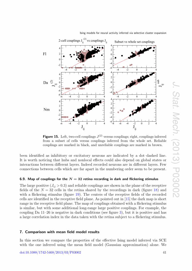
correlations pij(∆t) on a fixed time scale ∆t, which goes in this direction by reproducingneural activity observed in the data beyond that which was used to infer the model.This approach was introduced to analyze retinal data in [3, 4]. In section 7 we clarifythe relationship between the couplings Jij inferred by the Ising approach and the two-cell
approximation J(2)ij derived from cross-correlation analysis. The Ising model we apply in
the following aims to go beyond cross-correlation analysis in the sense that it disentanglesdirect couplings from correlations, correcting for network effects.
1.3. Ising model encoding of the activity
Neural activity represented in the form of spike trains can also be encoded in a binaryform. We first divide the total time interval of a recording of the activity into small timebins of size ∆t. The activity is then represented by set of binary variables sτi , hereaftercalled spins, where τ = 1, . . . , B labels the time bin and i = 1, . . . , N is a label which refersto a particular neuron. In the data we consider N spans a few decades (30–120). If in binτ neuron i has spiked at least once then we set sτi = 1, otherwise sτi = 0.
Ising models for neural activity inferred via selective cluster expansion
We write the probability of an N -spin configuration PN [s] in the data as the fraction ofbins carrying that configuration s = {s1, s2, . . . , sN}, and define the empirical HamiltonianHN [s] as minus the logarithm of PN . By definition, the Gibbs measure corresponding tothis Hamiltonian reproduces the data exactly. As the spins are binary variables, HN canbe expanded in full generality as
HN [s] = −N∑k=0
∑i1<i2<···<ip
J(k)i1,i2,...,ip
si1 si2 . . . sip , (3)
where J (0) is simply a constant ensuring the normalization of PN . Notice that, given anexperimental multielectrode recording, PN and HN depend on the binning interval ∆t.Knowledge of the 2N coefficients J in (3) is equivalent to specifying the probability ofeach one of the spin configurations. The model defined by (3) provides a complete, butflawed, representation of the experimental data. First, it gives a poor compression of thedata, requiring a number of variables which grows exponentially with the system size toexhaustively encode the probability of every configuration of the system. As a predictivemodel of the future behavior of the experimental system, it will also likely perform poorlycompared to other reasonable models due to the overfitting of the data.
It is tempting then to look for simpler approximate expressions of HN that retainmost of the statistical structure of the spin configurations. A sensible approximation tothe true interaction model should at least reproduce the values of the empirical one- andtwo-point correlation functions,
pi =1
B
B∑τ=1
sτi , pij =1
B
B∑τ=1
sτi sτj . (4)
These constraints can be satisfied by the Ising model defined by the Hamiltonian
H2[s] = −N∑i=1
hi si −∑i<j
Jij si sj. (5)
The corresponding probability of a configuration in the Ising model is given by thestandard equilibrium Gibbs measure,
P [s] =e−H2[s]
Z[{hi}, {Jij}], (6)
where the partition function Z[{hi}, {Jij}] =∑
s e−H2[s] ensures that∑
sP [s] = 1.The local fields {hi} and pairwise couplings {Jij} are the natural parameters
for encoding the one- and two-point correlations because they are the conjugatethermodynamical variables to these correlations. Indeed, the N (N + 1)/2 coupledequations (4) can be solved by finding the couplings and fields which minimize the cross-entropy between the inferred Ising model and the data
Ising models for neural activity inferred via selective cluster expansion
This can be verified by computing the derivatives of S∗[{hi}, {Ji,j}] with respect to thecouplings and fields,
∂S∗[{hi}, {Jij}]∂hi
=1
Z
∑s
sie−H2[s] − pi, (8)
∂S∗[{hi}, {Jij}]∂Jij
=1
Z
∑s
si sje−H2[s] − pij. (9)
At the minimum of (7) the derivatives must vanish, implying that the conditions (4) aresatisfied. Moreover, the minimal cross-entropy S2[{pi}, {pij}] = min{hi},{Jij}S
∗[{hi}, {Ji,j}]is the Legendre transform of the free energy F = − logZ[{hi}, {Jij}] of the Ising model.It can be shown (see [21]) that the Ising model (6) is the probabilistic model with themaximum entropy
S[P ] = −∑s
P [s] lnP [s] (10)
which satisfies the constraints that the average value of the one- and two-point correlationscoincide with the observed data (4) and that the probability distribution P [s] is normalizedsuch that all probabilities sum to one.
1.4. Previous results of the inverse Ising approach
It was put forward in [3, 37] that the Ising model defined by (6) not only reproducesthe one- and two-point firing correlations extracted from the data, it also captures otherfeatures of the data such as higher order correlations and multi-neuron firing frequencies.Thus the energy H2 provides a good approximation to the whole energy HN ; interactionsinvolving three or more spins in (3) are not quantitatively important, and it suffices to keepin the expansion local fields and pair interactions only. Further simplification, however, isnot generally possible. Hamiltonians H1 with no multi-spin interactions, corresponding tosetting all Jij = 0 in (5) with the fields hi chosen to reproduce the average neural activity,provide a very poor approximation to (3). Such independent neuron approximations failto reproduce, for example, the probability that k cells spike together in the same bin fork = 1, . . . , N .
The claim in [3, 37] is based on the following points:
• Information-theoretical arguments: call S1 the entropy of the independent neuronmodel H1, S2 the entropy of the Ising model (5), and SN the entropy of theexperimental distribution PN . Then the reduction in entropy of spin configurationscoming from pair correlations, I2 = S1 − S2, explains much of the reduction inentropy coming from correlations at all orders (or multi-information), IN = S1 − SN :I2/IN ' 90% [3]. Hence higher order correlations do not contribute much to the multi-information, implying that most of the correlation observed in the data is explainedsimply through pairwise interactions.
• The multi-neuron firing frequencies, i.e. the probability of k neurons spiking togetherin the same bin, predicted by the Ising model with pairwise interactions, are muchcloser to the experimental values than those of its independent cell counterpart.
• Higher order correlations (three spin and higher correlations) predicted by the Isingmodel are in good agreement with the experimental data.
Ising models for neural activity inferred via selective cluster expansion
2. Statistical effects of finite sampling
Finite sampling of the experimental systems we consider here introduces fluctuationswhich complicate the inverse problem. In this section we discuss the effects of finitesampling noise on the empirical one- and two-point correlations, consequences for theinference procedure, and statistical errors on the inferred couplings and fields.
2.1. Statistical error on empirical correlations
The inverse Ising approach requires measurements of the probability that each cell spikesin a time bin pi(∆t) and that each pair of cells spikes in the same time bin pij(∆t). Theseprobabilities can be obtained from the spike train data by counting the number of timewindows in which a cell, or two cells for the pair correlations, are active, divided by thetotal number of time windows B. It is important to notice that the number of sampledconfigurations, while large (typically the total recording time is of the order of one hour,which with a time bin of 20 ms corresponds to roughly 106 configurations), is limited.Therefore, the empirical correlations {pi}, {pij} we obtain will differ from the ones whichwould be obtained with an infinite sampling {ptrue
i }, {ptrueij } by typical fluctuations of the
order of {δpi}, {δpij}, which we estimate in the following.In our model, the spins are stochastic variables with Gibbs average
〈si〉 = ptruei (11)
and with variance
σi = 〈s2i 〉 − 〈si〉2 = ptrue
i (1− ptruei ). (12)
Their average pi over B independent samples is also a stochastic variable with the sameaverage as above, but with the standard deviation
δpi =
√ptruei (1− ptrue
i )
B'√pi(1− pi)
B, (13)
where in the last expression of (13) we have replaced the Gibbs average ptruei with the
empirical average, neglecting terms of the order 1/B2. Similarly, the pair correlationshave the average value
〈si sj〉 = ptrueij , (14)
and variance
σij = ptrueij (1− ptrue
ij ); (15)
therefore, their sampled average over B samples pij has a standard deviation
δpij '√pij(1− pij)
B. (16)
2.2. The Hessian of the cross-entropy: the importance of regularization terms
Because of finite sampling problems the fields and couplings obtained as minimizers of (7)are not necessarily well defined. As a simple example consider a single neuron (N = 1)
Ising models for neural activity inferred via selective cluster expansion
with an average spiking rate r. The probability that the corresponding spin in the binaryrepresentation is zero is exp(−r∆t) ' 1− r∆t, which is close to one for small bin widths∆t. If the number B of bins is much smaller than 1/(r∆t) the spin is likely to be equalto zero in all configurations. Hence p = 0 and the field solution of the inverse problemis h = −∞. In practice, the number B of available data is large enough to avoid thisdifficulty as far as single site probabilities are concerned. However, when two or more spinsare considered and higher order correlations are taken into account incomplete samplingcannot be avoided; some groups of cells are never active simultaneously, which leads toinfinite couplings.
This problem is easily cured with a Bayesian approach. We now start with a set ofdata consisting of B configurations of spins {sτ}, τ = 1, . . . , B, and assume that the datacome from the Ising model with Hamiltonian (5). The probability or likelihood of a spinconfiguration is given by (6). The likelihood of the whole set of data is therefore
where the cross-entropy S∗ is defined in (7).In order to calculate the a posteriori probability of the couplings and fields we need
to introduce a prior probability over those parameters. In the absence of any information(data), let us assume that the couplings have a Gaussian distribution, with zero mean andvariance σ2,
Pprior[{hi}, {Jij}] = (2πσ2)−N(N+1)/2 exp
[− 1
2σ2
(∑i<j
J2ij
)]. (18)
So far, the variance is an unknown parameter. We expect it to be of the order of unity,that is, much smaller than the number of configurations B in the data set. Multiplying(17) and (18) leads to the Bayesian a posteriori probability for the fields and couplingsgiven the data,
Ppost[{hi}, {Jij}|{sτ}] =Pprior[{hi}, {Jij}]× P like[{sτ}|{hi}, {Jkl}]
P [{sτ}], (19)
where P [{sτ}] is a normalization constant which is independent of the couplings and fields.The most likely values for the fields and couplings are obtained by maximizing (19), thatis, by minimizing the modified cross-entropy,
S∗[{hi}, {Jij}, γ] = S∗[{hi}, {Jij}] +γ
2
(∑i<j
J2ij
), (20)
where
γ =1
B σ2. (21)
The value of the variance σ2 can be determined, once again, using a Bayesian criterion.P [{sτ}] in (19) is the a priori probability of the data set over all possible Ising models.The optimal variance is the one maximizing this quantity. The approach is illustrated in
Ising models for neural activity inferred via selective cluster expansion
detail in the simplest case of a single neuron, then extended to the case of interactingneurons in the appendix.
The precise form of the regularization term is somewhat arbitrary. For convenience inthe calculations we use the regularization
γ∑i<j
pi(1− pi)pj(1− pj) J2ij. (22)
This choice corresponds to a Gaussian prior for the interactions in a Bayesian framework.Another regularization term we use is based on the L1 norm rather than L2, and favorssparse coupling networks, i.e. with many couplings equal to zero,
γ∑i<j
√pi(1− pi)pj(1− pj)|Jij|, (23)
which corresponds to a Laplacian prior distribution. In section 7 we describe the propertiesof the L1 and L2 norm penalties in more detail, and in section 4.1 we motivate the pi, pijdependence of the terms in the regularization.
When the number of samples B in the data set becomes large, (21) shows that theregularization strength γ → 0; the couplings and fields determined by minimizing (7)always coincide with Bayes predictions in the perfect sampling limit. For finite B thepresence of a quadratic contribution in (20) ensures that S∗ grows rapidly far from theorigin along any direction in the N(N + 1)/2-dimensional space of fields and couplings.
Because of the regularization there exists a unique and finite minimizer of the cross-entropy. The Hessian matrix χ of the cross-entropy S∗, also called the Fisher informationmatrix, is given by
where 〈·〉 denotes the Gibbs average with measure (6), and i = 1, . . . , N , 1 ≤ k < l ≤ N .The addition of a regularization term with a quadratic penalty on the couplings andfields adds γ times the identity matrix to the Hessian, and as the unregularized χ isa covariance matrix and hence non-negative4, this assures that the susceptibility of theregularized model is positive definite. Thus S∗[{hi}, {Jij}, γ] is strictly convex. This provesthe existence and uniqueness of the solution to the inverse problem.
4 Let ~v = (~x, ~y) where ~x = (x1, x2, . . . , xN ) and ~y = (y12, y13, . . . , yN−1,N ) are, respectively N - and N(N − 1)/2-dimensional vectors. Then
Ising models for neural activity inferred via selective cluster expansion
2.3. Statistical error on couplings and fields
In this section we compute the statistical fluctuations of the inferred couplings and fieldsdue to finite sampling of the experimental system.
As in section 2.1, let us assume that data are not extracted from experiments butrather generated from the Ising model (5) with the fields {h∗i } and couplings {J∗ij} whichminimize the cross-entropy (7). From section 2.2 the probability of inferring a set of fields{hi} and couplings {Jij} is proportional to exp(−B S∗[{hi}, {Jij}]). When B is very large,this probability is tightly concentrated around the minimum of S∗, that is, {h∗i }, {J∗ij}.The difference between the inferred and the true fields and couplings is encoded in theN(N+1)/2-dimensional vector ~∆h,J of components {hi−h∗i }, {Jij−J∗ij}. The distributionof this vector is asymptotically Gaussian,
P [~∆h,J ] '√
detχ
(2πB)N(N+1)/4exp
(−B
2~∆†h,J · χ · ~∆h,J
). (25)
Statistical fluctuations of the couplings and fields are therefore characterized by thestandard deviations
δhi =
√1
B(χ−1)i,i, δJij =
√1
B(χ−1)ij,ij. (26)
Note that (13) and (16) can be also directly obtained from the covariance matrix χ.Indeed linear response theory tells us that
~∆p,c = χ · ~∆h,J . (27)
We deduce from (25) that ~∆p,c obeys a Gaussian distribution as ~∆h,J , with the Hessianmatrix χ replaced with its inverse matrix in (25). The typical uncertainties of the one- andtwo-point correlations are given by δpi =
√(1/B)(χ)i,i and δpij =
√(1/B)(χ)ij,ij, which
correspond exactly to (13) and (16).
3. The difficulty of the inverse Ising problem
The inverse problem can be subdivided into three different problems, which are ofincreasing difficulty [20].
Reconstruction of the interaction graph
It is possible to reproduce qualitative features of the underlying interaction graph (i.e. theset of interactions which would be inferred if the inverse problem was solved exactly),such as the number of connections to a given cell or the range of interactions, withoutdetermining the values of the couplings precisely. Knowing the rank of the couplings inabsolute value, for instance, gives an idea of the structure of the interaction graph. We willsee in section 7 that mean field approximations are only useful for finding precisely thenetwork of interactions in the case of weak interactions and not, as in the majority of theanalyzed neural data, for a dilute network with large couplings. These approximationsgenerally give, then, wrong values for the couplings but respect the ranking of largecouplings by magnitude, thereby allowing for the accurate recovery of the structure ofthe interaction graph of large couplings.
Ising models for neural activity inferred via selective cluster expansion
Reconstruction of the interaction graph and values of the couplings
It can be of interest to infer the values of the couplings more precisely, and to identifyreliable couplings, which are different from zero even when taking into account statisticalfluctuations due to finite sampling (26), and unreliable couplings which are compatiblewith zero. A precise inference of the value of the couplings compared with the error bar willbe helpful to characterize changes in the values of couplings, which can occur for example ina memory task [30]. Also, it would be of interest to characterize reliable negative couplingswith the aim of identifying inhibitory connections, which are particularly susceptible tosampling noise and thus difficult to assign reliably.
It has been pointed out in [21] that the difficulty of the inference problem dependson the inverse of the Fisher information matrix χ−1 (24). Whereas the susceptibility χcharacterizes the response of the Ising model to a small change in the couplings or fields,the inverse susceptibility χ−1 gives the change in the inferred couplings and fields due toa perturbation of the observed frequencies or correlations. If data are generated by sparsenetworks and if the sampling is good, then χ−1 is localized, i.e. it decays fast with thelength of the interaction path between spins in the interaction network. This propertyholds even in the presence of long-range correlations and makes the inverse problem notintrinsically hard.
It is important to notice that the sampling fluctuations in frequencies (13) andcorrelations (16) do not come from a sparse network structure and thus χ−1 can loseits localized properties because of sampling noise. In other words, overfitting can generatevery complicated and densely connected networks, which will have a large coupling-susceptibility. A way to filter the data must then be found to efficiently solve the inverseproblem in the presence of sampling noise. The selective cluster expansion, which weintroduce in section 5, approaches this problem by including methods of regularizationand by building up a solution to the inference problem in a progressive way, includingonly terms which contribute significantly to the inference so as to avoid the overfitting ofnoise.
Reconstruction of the empirical correlations
The most difficult inference task is to find the local fields and the network of couplingswhich truly satisfy the minimum of (7), and which therefore reproduce the frequenciesand correlations obtained from data. One can use such an inferred Ising model to thenpredict, for example, the observed higher moments of the distributions (three body orhigher order correlations) or multi-neuron firing frequencies, as discussed in section 1.4.The Ising model could also be used to predict the response to a local perturbation, whichcould be due to a stimulation, or the ablation of a connection.
The reconstruction problem is difficult because a small change in the inferredparameters can result in large changes in the correlations and frequencies given by theinferred model. In other words, the susceptibility matrix may be dense, rather than sparse,with many large entries. Let again ~∆p,c denote the N(N + 1)/2-dimensional vector whosecomponents are the differences between the predicted and true values of the frequenciesand correlations. Typically inference errors come from the approximations made in theresolution of the inverse problem. Using the linear response theory of (27) we can estimate
Ising models for neural activity inferred via selective cluster expansion
the order of magnitude of the reconstruction error due to an inference error:
~∆p,c ≈ |χ|~∆h,J , (28)
where |χ| is the norm of the matrix defined as the sum over the rows of the maximumelement over the columns,
|χ| =∑i
maxjχi,j. (29)
Let us imagine that a parameter hi has been inferred with an inference error ofthe order ∆h ' 0.1, which is a typical order of magnitude of the expected statisticalfluctuations in the inferred parameters. This inference error can drastically change thereconstructed pi. For example, for the recording of N = 40 neurons in the retina subjectto a natural movie stimulus [3] |χ| = 0.6, and the consequent δp ≈ 0.06 is of the sameorder of magnitude as the pi, which is much larger than the statistical errors we expecton these variables. We discuss in section 6 how the reconstruction behaves as a functionof the inference precision in the cluster expansion. This example explains why even if thenetwork is reconstructed at the precision corresponding to the statistical fluctuations (26)we expect from the finite sampling, and therefore the inverse problem is quite accuratelysolved, the statistical properties of the data on the inferred model can be much harder toreproduce and may require sophisticated expansion and fine tuning of some parameters.
Note that equation (28) gives only an order of magnitude; the more precise matrixdependence of the response in (27) tells us that the modes which correspond to largeeigenvalues of the Hessian matrix χ have to be more precisely determined to solve thereconstruction problem well, while the others, which correspond to small eigenvalues ofthe Hessian matrix, have less impact on the reconstruction problem.
4. High temperature expansions and the mean field entropy SMF
The main problem of the minimization of the cross-entropy S∗ (7) is the calculationof the partition function Z, which, if done exactly, requires the sum over all 2N possibleconfigurations of the system of N spins. Because this sum becomes prohibitive for systemswith more than ≈20 spins some approximate solution of the inverse problem must befound.
High temperature expansions [14], [38]–[40] of the Legendre transform of thefree energy are useful when the pairs of variables interact through weak couplings.The Ising model with weak (of the order of N−1/2) interactions is the so-calledSherrington–Kirkpatrick model. In this case the entropy S[{pi}, {pij}] coincidesasymptotically for large N with
Ising models for neural activity inferred via selective cluster expansion
is the entropy of independent spin variables with averages {pi}, and
Mij[{pi}, {pij}] =pij − pipj√
pi(1− pi)pj(1− pj), (32)
which can be calculated in O(N3) time [14, 41], and is consistent with the so-called TAPequations [42]. It is important to underline that what we call the mean field entropy SMF
corresponds to the entropy of a Gaussian model of continuous spin variables with averagespi and variances pi (1− pi).
The derivatives of SMF with respect to the {pij} and {pi} give the values of thecouplings and fields,
(JMF)ij = −∂SMF
∂pij= − (M−1)ij√
pi(1− pi)pj(1− pj),
(hMF)i = −∂SMF
∂pi=∑j(6=i)
(JMF )ij
(cij
pi − 1/2
pi(1− pi)− pj
),
(33)
where cij = pij − pipj is the connected correlation.It is possible to get an idea of the goodness of the high temperature expansion from
the size of the correlation indices CIij = pij/(pipj), which are the expansion parametersof the high temperature series [14]. We note that in neural data, even if the connectedcorrelations are small, the correlation indices CIij can be large because the probabilitiespi, pj that individual cells are active in a time bin are also generally small, and CIij is oforder one. Histograms of the correlation indices for the different data sets we analyze areshown in figures 13 and 14, and show that the correlation indices are small in absolutevalue (|CIij| ≤ 2.2) only in the data sets of in vivo recordings of the medial prefrontalcortex of rats with tetrodes [31, 33]. We therefore expect the high temperature expansionand in particular SMF to be a good approximation to the inverse problem only for thisdata set.
4.1. L2-regularized mean field entropy
A regularized version of the mean field entropy can be computed analytically [21]. Thederivation is as follows. First we use the mean field expression for the cross-entropy atfixed couplings Jij and frequencies pi (see [39]) to rewrite
SIsing[{pi}, {Jij}] = Sind[{pi}]− 12
log det (Id− J ′)−∑i<j
Jij (pij − pi pj), (34)
where J ′ij = Jij√pi(1− pi)pj(1− pj) and Id denotes the N -dimensional identity matrix.
We consider the L2-norm regularization (22). The entropy at fixed data {pi}, {pij} is
Ising models for neural activity inferred via selective cluster expansion
where M [{pi}, {pij}] is defined in (32). The optimal interaction matrix J ′ is the root ofthe equation
(Id− J ′)−1 −M [{pi}, {pij}] + γ J ′ = 0. (36)
Hence, J ′ has the same eigenvectors as M [{pi}, {pij}], a consequence of the dependenceon pi we have chosen for the quadratic regularization term in (22). Let jq denote the qtheigenvalue of J ′. Then
SL2MF[{pi}, {pij}, γ] = Sind[{pi}] + 1
2
N∑q=1
(log mq + 1− mq) , (37)
where mq is the largest root of m2q − mq(mq − γ) = γ, and mq is the qth eigenvalue of
M [{pi}, {pij}]. Note that mq = mq when γ = 0, as expected.
4.2. L1-regularized mean field entropy
With the choice of an L1-norm regularization, the entropy at fixed data p becomes
SL1MF[{pi}, {pij}, γ] = Sind[{pi}] + min
{J ′ij}
[−1
2log det(Id− J ′)
− 12tr (J ′ ·M [{pi}, {pij}]) + γ
∑i<j
|J ′ij|]. (38)
No analytical expression exists for the optimal J ′. However, it can be found in a polynomialtime using convex optimization techniques. The minimization of (38) is known in thestatistics literature as the estimate of the precision matrix with a constraint of sparsity.Several numerical procedures to compute J ′ efficiently are available [43].
5. Selective cluster expansion
When an exact calculation of the partition function is out of reach, and the amplitudesof the correlation indices are large, an accurate estimate of the interactions which solvethe inverse Ising problem can be obtained through cluster expansions. Cluster expansionshave a rich history in statistical mechanics, e.g. the virial expansion in the theory of liquidsor cluster variational methods [44].
The selective cluster expansion algorithm (SCE) which we have recently proposed [20,21] makes use of an assumption about the properties of the inverse susceptibility χ−1
to efficiently generate an approximate solution to the inverse Ising inference problem.χ−1 is typically much sparser and shorter range than χ, implying that most interactionsinferred from a given set of data depend strongly on only a small set of correlations. Thusan estimate of the interactions for the entire system can be constructed by solving theinference problem on small subsets (clusters) of spins and combining the results. The SCEgives such an estimate by recursively solving the inverse Ising problem on small clustersof spins, selecting the clusters which give significant information about the underlyinginteraction graph according to their contribution to the entropy S of the inferred Isingmodel, and building from these a new set of clusters to analyze. At the end of this cluster
Ising models for neural activity inferred via selective cluster expansion
expansion procedure, an estimate of the entropy and of the interactions for the full systemis produced based on the values inferred on each cluster.
Let SΓ denote the entropy of the Ising model defined just on a subset Γ = {i1, i2, . . .}of the full set of spins, which reproduces the one- and two-point correlations obtainedfrom data for this subset. The entropy S of the inferred Ising model on the full system ofN spins can then be expanded formally as a sum of individual contributions from each ofthe 2N − 1 nonempty subsets,
S =∑
Γ
∆SΓ, ∆SΓ = SΓ −∑Γ′⊂Γ
∆SΓ′ . (39)
The cluster entropy ∆SΓ, defined recursively in (39), measures the contribution of thecluster Γ to the total entropy. It is calculated by subtracting the cluster entropies of allpossible smaller subsets of Γ from the subset entropy SΓ. Each cluster entropy dependsonly upon the correlations between the spins in that cluster, and for small clusters it iseasy to compute numerically. The contribution of each cluster to the interactions, whichwe denote ∆JΓ, is defined analogously and computed at the same time as the clusterentropy. The elements of JΓ are the couplings and fields which minimize the cross-entropyS∗ restricted to the cluster Γ. Note that in applications to real data, we employ some formof regularization (22), (23) to ensure that the Hessian χ is positive definite and to reducethe effects of sampling noise.
As an example, the entropy of a single-spin cluster is, using (39) with N = 1,
Using again (39) with N = 2, we obtain ∆S(i,j)[pi, pj, pij] = S(i,j)[pi, pj, pij] − ∆S(i)[pi] −∆S(j)[pj], which measures the loss in entropy when imposing the constraint 〈si sj〉 = pijon a system of two spins with fixed magnetizations, 〈si〉 = pi, 〈sj〉 = pj. The contributionto the field of the two-spin cluster is
Note that the two-cell couplings, which do not take into account network effects, reduceto the logarithm of the correlation index for pij � pi� 1, which is typically the case whenthe time bin is much smaller than the typical interval between spikes. In this case pi ∝ ∆t
Ising models for neural activity inferred via selective cluster expansion
and pij ∝ ∆t2, thus
J(2)ij ≈ log
pijpi pj
. (44)
It is difficult to write the entropy analytically for clusters of more than two spins, butSΓ can be computed numerically as the minimum of the cross-entropy (7). This involvescalculating Z, a sum over an exponential number of spin configurations. In practice thislimits the size of the clusters which we can consider to those with .20 spins.
A recursive use of (39), or the Mobius inversion formula, allows us to obtain ∆SΓ forlarger and larger clusters Γ (see also the pseudocode of algorithm 1). It is important tonote that the form of ∆S is such that the sum of all cluster entropies over all possiblesubsets, including the whole set, of a cluster Γ is just the total entropy of the cluster SΓ.The analogous result also holds for ∆J. This means in particular that by construction thesum over all possible clusters for the full system of N spins yields the exact entropy Sand interactions J.
It is also possible to perform an expansion in S−S0, where S0 is a ‘reference entropy’approximating S which we expand around. As with S, the reference entropy S0 shouldbe computable on all possible subsets of the system, and should depend only on the one-and two-point correlations of the spins in the subsets. Again, by the construction rule(39) and independent of the functional form of S0, summing over all the clusters will giveback the exact value of S − S0 for the full system. We will show in applications to neuraldata (see section 6) that it can be useful to consider an expansion S −SMF rather than Salone, using the mean field result as a reference entropy S0. In some cases the expansionof S − SMF converges much faster than the expansion of S alone.
The cluster entropy measures a cluster’s contribution to the total entropy, which couldnot be gained from its sub-clusters taken separately. Intuitively, we expect that clusterswith small |∆SΓ| contribute little new information about the underlying interaction graphwhich is not revealed by any of their subsets. Indeed, it has been shown [20, 21] that smallcluster entropies have a universal distribution, reflecting fluctuations in the experimentallyobserved correlations due to finite sampling (13) and (16). Cluster entropies that arenonzero due to real interactions between the constituent spins also tend to decrease inmagnitude as the cluster size becomes large, decaying exponentially in the size of theshortest closed interaction path between the spins in the cluster. In the SCE therefore allclusters which have |∆SΓ| smaller than a fixed threshold T are discarded. Selecting onlythose clusters which have cluster entropies larger than a chosen threshold helps to avoidthe overfitting of noisy data.
Clearly, it is not possible to compute all of the 2N −1 cluster entropies, correspondingto all the nonempty subsets of the full set of spins, even for rather small systems. Tomake the algorithm computationally feasible we must have a method for truncating thecluster expansion. This is implemented in the SCE by a recursive construction rule for theclusters included in the expansion (see the pseudocode of algorithm 2). We begin with thecomputation of the cluster entropies for all N clusters of size k = 1. The contribution ofeach cluster to the interactions is also recorded for later use. Each subsequent step followsthe same pattern. First, clusters with |∆SΓ| < T are removed. We then include in thenext step of the expansion all clusters which are unions of two of the remaining clustersof size k, Γ′ = Γ1 ∪ Γ2, such that the new cluster Γ′ contains k + 1 spins.
Ising models for neural activity inferred via selective cluster expansion
The expansion naturally terminates when no more new clusters can be formed. Thisapproach prevents a combinatorial explosion of the number of clusters considered in theexpansion. It is also consistent with the idea of exploring paths of strong interactions inthe interaction graph, as new clusters are built up from smaller clusters which have alreadybeen found to have significant interactions and which share many spins in common. Finalestimates for the entropy and the interactions are obtained by adding up all of the ∆SΓ
and ∆JΓ. Contributions of S0 and J0 are also added if the reference entropy is used in theexpansion.
5.1. Pseudocode of the cluster algorithm
In this section we present pseudo-codes useful for the practical implementation of theinference algorithm, following [20].
The principal routine of the cluster algorithm is the iterative computation of thecluster entropy, given in algorithm 1. When the routine to compute the entropies of various
Algorithm 1 Computation of cluster entropy ∆S(Γ)
Require: Γ (of size K), p, routines to calculate S0 and S∆SΓ ← SΓ − S0,Γ
for SIZE = K − 1 to 1 dofor every Γ′ with SIZE spins in Γ do
∆SΓ ← ∆SΓ −∆SΓ′
end forend for
Output: ∆SΓ
clusters is called several times a substantial speed-up can be achieved by memorizing theentropies ∆SΓ of every cluster. In section 5.2, we will discuss how to calculate the subsetentropy SΓ in more detail.
In section 6, we discuss the performance of the algorithm and compare the results inof the expansion in S alone, i.e. with no S0,Γ, and with a mean field reference entropy (30)
S0,Γ = SL2MF,Γ obtained using an L2 norm regularization (37) and S0,Γ = SL1
MF,Γ using an L1
norm regularization (38) on the couplings {Jij}.The core of our inference algorithm is the recursive building-up and the selection of
new clusters, described in algorithm 2. The threshold T , which establishes which clusterswill be kept in the expansion, is a parameter which is fixed in a run of the selective clusteralgorithm. The choice of the optimal threshold T ∗ is discussed in the section 5.3.
5.2. Numerical optimization of the cluster algorithm
In this section we review some of the computational challenges of the algorithm andnumerical methods for running the algorithm efficiently.
The primary computational bottleneck of the selective cluster expansion algorithm isthe repeated solution of the inverse Ising problem and the computation of the entropyon each K-spin system included in the expansion, which is used to calculate the clusterentropy (see algorithm 1).
Ising models for neural activity inferred via selective cluster expansion
Algorithm 2 Adaptive cluster expansion
Require: N , T , S0, routine to calculate ∆SΓ from pLIST ← ∅ {All selected clusters}SIZE ← 1LIST(1) ← (1) ∪ (2) ∪ . . . ∪ (N) {Clusters of SIZE=1}repeat {Building-up of clusters with one more spin}
LIST ← LIST ∪ LIST(SIZE) {Store current clusters}LIST(SIZE+1) ← ∅for every pair Γ1,Γ2 ∈ LIST(SIZE) do
ΓI ← Γ1 ∩ Γ2 {Spins belonging to Γ1 and to Γ2}ΓU ← Γ1 ∪ Γ2 {Spins belonging to Γ1 or to Γ2}if ΓI contains (SIZE-1) spins and |∆SΓU
| > T thenLIST(SIZE+1)← LIST(SIZE+1) ∪ ΓU {add ΓU to the list of selected clusters}
end ifend forSIZE ← SIZE+1
until LIST(SIZE) = ∅S ← S0, J ← − d
dpS0 {Calculation of S, J}
for Γ ∈ LIST doS ← S + ∆SΓ, J← J− d
dp∆SΓ
end forOutput: S, J and LIST of clusters
Given a cluster Γ the partition function of the K-spin system restricted to Γ,
Z[{hi}, {Jij},Γ] =∑
{si=0,1; i∈Γ}
exp
∑i∈Γ
hi si +∑
i<j; i,j∈Γ
Jij si sj
, (45)
can be computed in time∝2K . Then one has to find the most likely set of {Jij} and {hi} foreach cluster given the experimental data, that is, we must solve the convex optimizationproblem
min{hi},{Jij}
S∗[{hi}, {Jij},Γ] = logZ[{hi}, {Jij},Γ]−∑i∈Γ
hi pi −∑
i<j; i,j∈Γ
Jij pij
. (46)
No analytical solution exists for clusters of more than a few spins. As a single run ofthe cluster expansion algorithm may include thousands or even millions of clusters, it iscritically important that the optimization problem (46) be solved as quickly as possible.
Given a starting value for the {Jij} and {hi}, we employ a hybrid approach whichcombines the standard optimization techniques of gradient descent and Newton’s methodto step progressively closer to the minimum. Gradient descent steps are chosen along thedirection of steepest descent, while Newton’s method specifies a step direction towardsthe minimum of a local quadratic approximation of S∗. When far from the minimum, weuse gradient descent for its computational simplicity and numerical stability. Once the{Jij} and {hi} are determined to be close to the values which solve (46), we switch to
Ising models for neural activity inferred via selective cluster expansion
Newton’s method, which requires more computational resources but has a much betterrate of convergence close to the minimum [45].
A careful choice of the initial conditions is also essential for obtaining a fast solutionwith minimal computational effort. We begin the optimization problem with an initialguess for {Jij} and {hi} based upon the assumption that the couplings and fieldsminimizing S∗ will be similar to those that were found for smaller clusters containingthe same sites. In many cases this initial guess works very well, and the optimizationroutine may find the minimum with just a single step. Just including this choice for theinitial interactions can cut the total running time of the algorithm in half.
As described in section 2.2, we may regularize the couplings {Jij} by adding a penaltyterm to S∗ for each coupling which is nonzero. Regularization is useful for controllingspurious large couplings that arise from noise or undersampling of the experimentalsystem, as well as ensuring the convexity of the Hessian χ, so that the inference problemhas a unique minimum at a finite value of the couplings. Common choices of the penaltyare based on the L1-norm
γ∑i<j
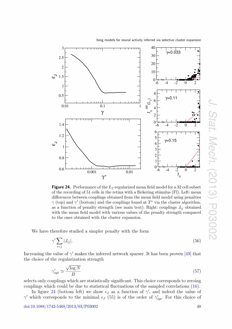
√pi(1− pi)pj(1− pj)|Jij| (47)
or the L2-norm
γ∑i<j
pi(1− pi)pj(1− pj) J2ij. (48)
Such terms are natural in the context of Bayesian inference. The addition of (47) to S∗ isequivalent to assuming a Laplacian prior distribution for the couplings, while the L2-normpenalty (48) corresponds to a Gaussian prior. Typically we take γ ≈ 1/(10B p2(1− p)2),where p is the average spiking frequency for a given data set.
Use of the L1-norm penalty makes the optimization problem more difficult, as thefunction to be minimized is no longer smooth. In particular, in this case the gradient ofS∗ is undefined when any of the couplings Jij = 0. To overcome the lack of differentiabilityof S∗ we use a modified version of the projected scaled sub-gradient method of [46]. Thismethod makes use of the sub-gradient, a generalization of the gradient which is welldefined even when some couplings are zero. It also allows couplings to be set exactly tozero during the step process, unlike a typical gradient descent or Newton’s method step.Despite these additional complexities, the optimization problem including the L1-normpenalty can be solved with similar speed and accuracy as in the L2-norm regularized orunregularized case.
5.3. Convergence and choice of the threshold T ∗
In the following we describe the practical procedure for applying the inference algorithmto a set of data. Because we do not know a priori the optimal value of the threshold T ∗
we run the algorithm at different values of the threshold following the iterative heuristicbelow:
• Start with a large value of the threshold T , typically T = 1, at which only single-spinclusters are selected.
• Infer the fields and the couplings at that threshold.
Ising models for neural activity inferred via selective cluster expansion
• If the number of selected clusters has changed with respect to the previous value ofthe threshold, run a Monte Carlo simulation to check the reconstruction of the firstand second moments. From the Monte Carlo simulation we obtain {prec
i }, {precij } and
calculate the relative errors on the reconstructed averages and connected correlationscrecij = prec
ij −preci prec
j with respect to their statistical fluctuations due to finite sampling,
εp =
(1
N
∑i
(preci − pi)2
(δpi)2
)1/2
, εc =
(2
N (N − 1)
∑i<j
(crecij − cij)2
(δcij)2
)1/2
. (49)
The denominators in (49) measure the typical fluctuations of the data expected atthermal equilibrium (see (13) and (16)), and
δcij = δpij + piδpj + pjδpi. (50)
• Iterate this procedure by lowering the threshold T and stopping when the errors εp ' 1,εc ' 1. The corresponding value of the threshold is the optimal threshold T ∗.
• Assign error bars to the inferred couplings and fields using (26).
Note that T ∗ is chosen as the first value of the threshold such that εp ' 1, εc ' 1in order to reconstruct the data with the simplest possible network of interactions,i.e. that which has the smallest inverse susceptibility. Through the cluster expansionone ‘fills in’ entries of the inverse susceptibility matrix χ−1
ijkl = (∂Jij/∂ckl) of the inferredIsing model in a progressive way, starting with the largest contributions and stoppingwhen the one- and two-point correlations are reconstructed within the uncertaintyprovided by the finite sampling fluctuations. By decreasing the threshold, the numberof clusters which contribute to a given coupling increases, or in other words each inferredparameter {hi}, {Jij} depends on increasingly more experimental correlations, includingthose which are poorly sampled. As a consequence, even if the underlying interactionswhich have generated the data have a simple structure and a corresponding small inversesusceptibility, poorly sampled correlations may lead to reconstructed networks withcomplicated structure and large inverse susceptibility (see figures 5(D) and (E)). Thisis especially true for small correlations, where the sampling fluctuations (13) and (16) canbe of a similar order of magnitude to the correlations themselves. Decreasing the thresholdmore than is necessary to fit the one- and two-point correlations is undesirable, not onlybecause the complicated structure of interactions due to overfitting will not necessarilycorrespond well with the underlying interaction network, but also because progressivelylower values of the threshold increase the computational difficulty of the inference problem.
We note however that there is no risk of overfitting data which have been perfectlysampled. In this case, as there is no sampling noise, one is justified in fitting the model tothe data as tightly as is practically possible.
We now consider the typical pattern for the convergence of the reconstruction errorand its relationship with the convergence of the entropy expansion in more detail. Firstlet us imagine that the largest inference error is δhin
i on a field hi; the inference error onthe entropy δSin can be related to δhin
i because hi and pi are conjugate variables (see (6))and therefore (∂S/∂pi) = −hi, or
Ising models for neural activity inferred via selective cluster expansion
Figure 5. (A) Typical pattern of the relative reconstruction error εp for smallcorrelation lengths of the system, and without a reference entropy. At smallvalues of the threshold the reconstruction error decreases monotonically becausethe entropy expansion is absolutely convergent. Note that without the referenceentropy εp ∼ 0 at large values of the threshold, because when only clusters of sizeone are included in the expansion the fit is equivalent to that of an independentcell model and the experimental frequencies are matched perfectly. When εp ' 1(dashed line) and εc ' 1 (not shown) a network which is able to reproduce the datawithin the statistical uncertainties is found. At smaller values of the threshold,errors εp, εc < 1, corresponding to overfitting of the data. For systems which arevery well sampled (red line), the problem of overfitting is less severe. (B) Typicalpattern for εp for systems with longer correlation lengths; larger fluctuations ofεp, εc are present. (C) Thanks to the reference entropy the fluctuations of εp,εc at small threshold are smaller but εp at large threshold can be large. (D) Bylowering the threshold the susceptibility of the inverse problem increases: wereconstruct less and less sparse networks while making the inverse problem morecomputationally challenging. At small values of the threshold the relative errorscan become smaller than one, suggesting overfitting. When the data are overfitthe susceptibility of the inverse problem increases because the noise has no simplenetwork structure. (E) With the reference entropy at large values of the thresholdthe inverse susceptibility is nonzero even if the underlying interactions are shortrange, thanks to the properties of the Gaussian model [21].
The relationship between the convergence error on the fields and the reconstruction erroron the one- and two-point correlations is, as discussed in section 3, δpi ≈ |χ|δhi, where|χ| is the norm of the susceptibility matrix as defined in (29). Using (51) the order ofmagnitude of the typical reconstruction error is related to the convergence error of thecluster expansion,
Ising models for neural activity inferred via selective cluster expansion
where p is the average spiking probability of the cell populations for a given choice ofthe time bin. As mentioned in section 3, for |χ|/p small the reconstruction problem iseasy, while for |χ|/p large the reconstruction problem is difficult and small errors on theinferred parameters give large errors in the reconstructed observables. Reconstruction ofthe correlations within the sampling precision (13) requires
δprec
δp=|χ| δSin
√B
p√p(1− p)
≈ 1. (53)
The same reasoning holds for the reconstruction error εc, but again it gives only a roughestimate, because the matrix dependence of (27) has to be properly taken into account.A sketch of the typical pattern for the reconstruction errors by lowering the threshold Tis shown in figure 5.
To understand how the inference errors δhini , δJ
inij behave as a function of the threshold,
it is necessary to start from the understanding of the convergence of the cluster entropyexpansion as a function of the threshold. At large values of the threshold, importantclusters, corresponding to pairs with large correlation indices, are progressively addedup, resulting in a large change in the relative errors. As the threshold is lowered largefluctuations of the relative errors may still appear. As already discussed in [21], diluteinteraction networks display a cancellation property of the cluster entropies. Clusterswhich share the same interaction path, and which are not first neighbors in the couplingnetwork, have similar cluster entropies in absolute value but with different signs. When allof the cluster entropies corresponding to a given interaction path are summed, their overallcontribution is typically much smaller than the contribution of any individual cluster.Because such collections of clusters have cluster entropies which are similar in magnitude,they are typically added to the cluster expansion in packets when the threshold is lowered.Large fluctuations of the entropy error δSin arise when the threshold is chosen betweenthe largest and smallest values of the cluster entropies for clusters belonging to a giveninteraction path, thus ‘cutting’ the packet by including only part of the collection in theexpansion, such that the cluster entropies cannot cancel each other. Larger fluctuationsof the reconstruction error which are amplified by the direct susceptibility of the system(52) arise in correspondence to these values of the threshold.
As shown in [21] the entropy expansion can be absolutely convergent as the thresholdis lowered (see figure 5(A)). When the correlation length of the system is small δSin
decreases smoothly as the threshold is lowered. In contrast, when the correlation length ofthe system is large, fluctuations of δSin appear (see figure 5(B)). When taking SMF as thereference entropy, as shown in figure 5(C), the relative error of the one-point correlationsεp is not small even when the threshold is large; the network corresponding to SMF is nota network of independent spins, and the inverse susceptibility of the reconstructed systemis different from zero even for large values of the threshold (figure 5(D)). Fluctuations ofthe error at small values of the threshold are smaller, because the entropies of nonzerocluster entropies arising purely from sampling fluctuations (13) and (16) are smaller [21].
When a threshold T ∗ is reached such that the relevant clusters corresponding to thestructure of the inverse susceptibility matrix in the real interaction graph have beensummed up, the entropy error δSin goes to zero in the limit of perfect sampling. Forfinite sampling, it goes to a residual value corresponding to the difference between theentropy of the perfectly sampled system and the system which has been finitely sampled.
Ising models for neural activity inferred via selective cluster expansion
At such values of the threshold εp = εc ' 1. We have verified in the analyzed data sets thatthe inverse susceptibility χ−1 for the inferred Ising model at the threshold T ∗ is sparse. Forexample, for the retinal recording of 60 cells in dark conditions only 20% of the elementsof χ−1 are different from zero (within a precision of 10−9). However, we note that theconvergence of the expansion is not guaranteed. When the sampling noise, which has nosimple network structure, is very large, it can mix up different packets and obscure thestructure of the inferred interaction graph.
6. Application to real data
As an example of potential applications of the selective cluster expansion algorithm (SCE)we have re-analyzed, following [15], several sets of real data from multielectrode recordingsof collections of neurons. We examine in vitro recordings of salamander retinal ganglioncells.
• A 4450 s recording of 51 ganglion cells in a retina illuminated with randomly flickeringbright squares [22]. The recording is made with a multielectrode array on a surfaceof about 1 mm2, and approximately 20% of the ganglion cells on that surface arerecorded. The position of the receptive field of these cells is known.
• A 2000 s recording of the spontaneous activity of 60 cells of the same retina asabove observed in total darkness, of which 32 cells are common to the recordingwith randomly flickering stimulus [22].
• A recording of 40 cells in a salamander retina presented with a 120 s natural movierepeated 20 times. This recording is much denser; approximately 90% of the ganglioncells on the analyzed surface are recorded [3].
We also study several in vivo recordings of neurons in the medial prefrontal cortex ofa rat during a working memory task.
• A 1500 s recording of 37 cells with tetrodes, each consisting of four electrodes, whichrecord both superficial and deep layers of the medial prefrontal cortex [31].
• A 2800 s recording of 117 cells with silicon probes which record both superficial (layers2 and 3) and deep (layer 5) layers of the medial prefrontal cortex [30].
Figure 1 shows the raster plots displaying spike trains for the first second of recordingsof the different data sets. Unless otherwise indicated, the time bin we use to analyze thedata is ∆t = 20 ms. Spiking frequencies and pairwise correlations for a fixed time windoware shown in figures 9 and 10. We observe from these figures that in cortical data thefrequency of the activity is higher, and in particular some cells spike very rapidly. Theretinal recordings are stationary in the sense that the spiking frequencies and pairwisecorrelations of the data do not change over time. In the recordings with a natural moviestimulus this holds at least on a time scale larger than 120 s. The cortical data sets,however, are nonstationary. In particular, some cells are active only in part of the recordingof the 117 cells in medial prefrontal cortex, see figure 4. Note that in the analysis we presenthere data are considered to be stationary and the time dependence is not explicitly takeninto account. We discuss the consequences of this assumption for nonstationary data andhow to go beyond this limitation in the conclusion.
Ising models for neural activity inferred via selective cluster expansion
Figure 6. Performance of the SCE of S − SMF with L2 norm regularizationon retinal data as a function of the threshold T , analyzed with a time binof ∆t = 20 ms. The reconstruction errors εp (solid) and εc (dashed) (49) arecomputed from Monte Carlo simulations. The value ε = 1 is indicated by a reddotted line, and the selected optimal threshold T ∗ is marked in each plot with anarrow. Fl, flickering stimulus: left, whole set of 51 cells; right, subset of 32 cells.Da, dark: left, whole set of 60 cells; right, subset of 32 cells. Nm, natural moviestimulus: left, whole set of 40 cells; right, subset of 20 cells.
The correlation index histograms for some cells of the different data sets are shown infigures 2–4. As discussed in section 1.2, the correlation index is the expansion parameter inthe high temperature expansion, and when it is small, as for the N = 37 cortical data set(CA), it means that the interactions are weak and that SMF gives a good approximationof the couplings. This implies also that the cluster expansion, with or without a referenceentropy, will converge easily. When the correlation indices are large the magnitude ofthe couplings will be also be larger. In this case the convergence of the SCE and theoptimal expansion variable (i.e. S − SMF or S with no reference entropy) will depend onthe structure of the interactions. We explore this point in more detail below.
6.1. Performance of the algorithm for retinal data
We show the behavior of the reconstruction errors εp and εc as a function of the thresholdT on the retinal data in figure 6 for the expansion of S−SMF. Results on the convergenceof the algorithm and on the value of the inferred entropy are summarized in table 1for the different procedures tested, including expansions without the reference entropy.
Ising models for neural activity inferred via selective cluster expansion
These results include the value of the optimal threshold T ∗, as well as the size of thelargest cluster in the expansion Kmax, the total number of clusters processed Ntotcl, thetotal number of clusters selected at Ntotsel, and the inferred value of the entropy S, allevaluated at T ∗.
As shown in the figures and in the table, the reference entropy S0 is helpful for theinference problem when the SCE is applied to retinal data. The threshold T ∗ is lower forthe expansion of S alone with no S0, implying an increase in the number of processedclusters and a larger value for Kmax. For the flickering stimulus (Fl) the procedurewithout reference entropy did not converge even at a low value of the threshold. Heresmall couplings, which would have been obtained through the mean field couplings in theexpansion of S − SMF, are important for the proper reconstruction of the correlations,as mentioned in section 3. Decreasing the threshold enough to fit many small couplingsdrives the SCE algorithm to consider very large clusters (Kmax = 17 at the smallest valueof T tested), which slows the algorithm considerably.
Both L1 and L2 norm regularizations on S and SMF worked similarly well. In eachcase we found the value of Kmax to be around 6–8 and the threshold T ∗ varied between10−5 and 10−6.
We have also studied the inference problem on subsets of the full data sets describedabove. As shown in the right column of figure 6, the value of the threshold T ∗ and themaximum cluster size Kmax for large subsets of spins are of the same order of magnitudeas for the full set. Moreover, the number of clusters selected increases approximatelylinearly with the system size. This property was related in [20, 21] to the locality of thecoupling-susceptibility χ−1, and was shown to hold on artificial data of unidimensionaland bidimensional Ising models. This suggests that, for the chosen subset, the structureof the interaction graph has not changed much locally.
6.2. Performance of the algorithm for cortical data
In figure 7 we show the performance of the algorithm on cortical data, using no referenceentropy and with L1 regularization on the cluster entropies, and in table 1 we also givethe results for cases with L2 regularization and for the expansion of S−SMF. As expectedfrom the small values of the correlation indices, the SCE applied to the cortical recordingof N = 37 neurons (CA) works very well for expansions both with and without the meanfield reference entropy. Indeed, the expansion converges already at just Kmax = 2 with thereference entropy, and Kmax = 4 without it.
For the cortical recording of N = 117 cells we have tested the performance of thealgorithm with time bins of size ∆t = 5 ms (C5) and ∆t = 20 ms (CB). In both cases theconvergence of the algorithm was faster without the reference entropy (see table 2). Theconvergence of the algorithm for both ∆t = 20 ms and ∆t = 5 ms when expanding withrespect to the mean field reference entropy was very slow, and the relative errors εp, εcdid not approach one at a threshold T ≈ 10−7.
The poor performance of the expansion of S − SMF for cortical data, and the successof the expansion in S alone, is in stark contrast with the analysis of retinal recordings.This phenomenon is related to the fact that the interaction network which is capable offitting the cortical data is relatively dilute and consists of larger couplings, for whichthe mean field result is a poor approximation. The presence of a reference entropy
Ising models for neural activity inferred via selective cluster expansion
Figure 7. Performance of the SCE of S with L1 norm regularization on corticaldata as a function of the threshold T . The reconstruction errors εp (solid) andεc (dashed) (49) are computed from Monte Carlo simulations. The value ε = 1 isindicated by a red dotted line, and the selected optimal threshold T ∗ is markedin each plot with an arrow. CA, cortex recording of 37 cells analyzed with a timebin of 20 ms; CB, cortex recording of 117 cells analyzed with a time bin of 20 ms;C5, cortex recording of 117 cells analyzed with a time bin of 5 ms.
makes reconstructing the empirical correlations more difficult in this case, as the inferredinteraction network is then fully connected (even if many of these couplings are small).
As we expect from the fact that by increasing the time bin one unveils more of thenetwork structure and indirect couplings, the value of Kmax = 4 we obtain is smaller at∆t = 5 ms than at ∆t = 20 ms. Kmax = 10 is quite large in the latter case, indicating thatsome cells are connected with many others. This hub effect has been noted in [30, 47], andit can be related to the structure of the probes which record cells from different layers.For this data set, moreover, the value of Kmax and of the threshold T ∗ changes from thesubset of 30 neurons to the whole set, indicating a change in the local connectivity due tothe removal of many of the neurons in the full data set. A more detailed analysis of theinferred structure will be performed below.
6.3. Computational time at T ∗
As shown in figure 8, for all data sets for which the algorithm has converged, thecomputational time at the threshold T ∗ was not more than a few tens of minutes ofcalculation on a single core of a 2.8 GHz Intel i7 processor. The computational timeincreases with the number of processed clusters Ntotcl (see figure 8) and the maximum
Ising models for neural activity inferred via selective cluster expansion
Figure 8. Computational time of the SCE at threshold T ∗ for the different datasets as a function of the number of processed clusters Ntotcl. All times are forcomputations on one core of a 2.8 GHz Intel i7 processor. The computational timegrows with the number of processed clusters, which depends more strongly on thestructure of the interaction graph and on the number of sampled configurationsthan on the total system size N . For a fixed maximal size of clusters, Kmax, therunning time is roughly proportional to the number of clusters.
cluster size Kmax as
time 'Kmax∑K=1
Ntotcl(K) 2K , (54)
which is roughly proportional to the number of clusters given the same value of Kmax.However, when the number of clusters becomes large the construction rule can become
slow, and in fact this can become the limiting step for the computational time of thealgorithm. In the cluster construction step we test whether the union of each pair ofclusters of size K in the list of selected clusters forms a new cluster of size K + 1. Thetime necessary to complete this step thus scales quadratically with the number of selectedclusters, which may be quite large, particularly when expanding S without the referenceentropy S0. While the vast majority of attempts to form a new cluster may fail, the simpleact of checking each possibility becomes computationally demanding.
6.4. Reconstruction of the first and second moments of the activity
The spiking probabilities and connected correlations obtained from Monte Carlosimulations with the inferred parameters at T ∗ are close to those obtained fromexperiments as shown in figures 9–10. Indeed, the conditions εc = 1, εp = 1 specify thatthe difference between the inferred and empirical correlations is approximately the sameas the statistical uncertainty of the empirical correlations due to sampling a finite numberof configurations. We find that the reconstruction of the {pi} and {cij} is equally goodfor all the different reference entropy and regularization choices, provided of course thatthey reach the threshold T ∗ at which εc, εp = 1.
Ising models for neural activity inferred via selective cluster expansion
Figure 9. Spiking frequencies pi and connected correlations cij for retinal datasets calculated from a Monte Carlo simulation of the inferred Ising model(vertical) versus experimental values pexp
i , cexpij (horizontal). The error bars are
given by the statistical fluctuations δpi, δcij . Fl, flicker stimulus, 51 cells; Da,dark, 60 cells; Nm, natural movie stimulus, 40 cells.
6.5. Reconstruction of third moments and probability that k cells spike in the same timewindow
We have verified that the three-cell connected correlations cijk and the probability P (k)that k cells spike in the same bin are also quite well reproduced by the inferred Isingmodel, as shown in figures 11 and 12. Note that for the cortical recording of 37 cells (CA)and of 117 cells analyzed with ∆t = 5 ms (C5) the connected three-cell correlations arefor the majority of the cells so small that it is difficult to separate them from the samplingnoise. We have therefore also plotted the correlations pijk, which is the probability thatthe three cells spike in the same time bin, in figure 12. We emphasize that, unlike thereconstruction of the first and second moments, there are no a priori reasons that theIsing model should also reconstruct the higher moments of the experimental distribution,because it is not the true model which has generated the data, and these measurementsare not used as constraints in the inference. Nevertheless, as discussed in section 1.4 thismodel seems to reproduce fairly well the statistics of the data, at least for the cijk andthe P (k).
Intuitively, the reason for such a success may be simply due to the fact that thenumber of effective configurations that the system explores is 2S, and this number should
Ising models for neural activity inferred via selective cluster expansion
Figure 10. Spiking frequencies pi and connected correlations cij for corticaldata sets calculated from a Monte Carlo simulation of the inferred Ising model(vertical) versus experimental values pexp
i , cexpij (horizontal). The error bars are
given by the statistical fluctuations δpi, δcij .
be compared with the number of parameters N (N+1)/2 that we use to fit the distribution(see discussion in [15]). In principle, any model with a number of parameters similar tothe effective number of configurations could be equally good. For the data sets we haveanalyzed with N ≤ 60 (see tables 1 and 2), we have that N (N + 1)/2 > 2S. For largersystems with more than 100 cells, the exponential growth of 2S with N , due to the fact thatS ∝N , will be difficult to compensate with the increase of the number of parameters ∝N2.For the Fujisawa data sets with time bins of size 5 ms we have S = 5.9 so 2S < N (N+1)/2,but for 20 ms for we obtain N (N + 1)/2 = 6900 while 2S = 2.6 × 10⁴. Moreover, thereconstruction of the higher moments is still quite good. This could indicate that the Isingmodel, which is the maximal entropy model, is really a good model to reproduce the data.
6.6. Histogram of couplings, negative couplings and error bars on couplings
Once the couplings are inferred, the error bars δJij can be calculated from (26). Figures 13and 14 show the histogram of couplings in which we distinguish reliable couplings, forwhich |Jij|/δJij > 3, from unreliable couplings, which are compatible with zero within theerror bars. As expected, because of the sampling fluctuations there are many unreliablecouplings (particularly small couplings), but these may be still necessary to accuratelyreproduce the activity, as discussed in section 3. Large reliable couplings correspondgenerally to large correlation indices (see the cross-correlation histograms in figure 2),but the converse is not necessarily true.
An interesting issue is to separate inhibitory and excitatory connections. It isimportant to notice that negative couplings can be due to undersampling. Indeed, as
Ising models for neural activity inferred via selective cluster expansion
Figure 11. Reconstructed three-cell connected correlations cijk (vertical), andprobability P (k) that k cells spike in the same time bin (black), versus theexperimental ones cexp
ijk (horizontal) and P exp(k) (red) for retinal data. Thereconstructed values are obtained from a Monte Carlo simulation of the inferredIsing model. Fl, flicker stimulus, 51 cells; Da, dark, 60 cells; Nm, natural moviestimulus, 40 cells.
already noted, they can correspond to cells which never spike together in the recordedactivity, but often these couplings also have large error bars and therefore will be classifiedas unreliable (see the histograms in figures 13 and 14). Therefore, to properly define reliablenegative couplings it is important to know the error bars on the inferred couplings.
As shown in the histograms figures 13 and 14 in both retinal and cortical data thereare some large negative couplings which are reliable. There are fewer reliable large negativecouplings in dark and flicker retinal data, which can be related to the fact the majorityof the recorded cells in these data sets are of OFF cells.
In figure 3 we show the cross-correlation histograms of pairs of cells correspondingto negative couplings. Cells with negative couplings can correspond to those with a largecentral anticorrelation peak and a large correlation index, as is the case for Da 11–26, orthey can display a small negative correlation index as in the example of Fli 3–18, whichis perhaps attributable to network effects. Negative couplings can also be due to the factthat the Ising approach reproduces pairwise correlations in a fixed time bin and does notinclude the delay in response between neurons. Some couplings can change sign when thebin size is changed, as shown in the example of Fli 1–22, which displays a correlationpeak shifted by about 33 ms with respect to zero. As noted in [15], the corresponding pairrecorded in dark conditions has an unshifted peak and the inferred coupling is positive.Another case which is present in the N = 117 cortical recording is the pair CB 135–178,shown in figure 4, which has a negative coupling and a negative cross-correlation index
Ising models for neural activity inferred via selective cluster expansion
Figure 12. Reconstructed three-cell correlations pijk and connected correlationscijk (vertical), and probability P (k) that k cells spike in the same time bin (black)versus the experimental ones pexp
ijk , cexpijk (horizontal) and P exp(k) (red) for cortical
data. The reconstructed values are obtained from a Monte Carlo simulation ofthe inferred Ising model. CA, cortex recording of 37 cells; CB, cortex recordingof 117 cells analyzed with a time bin of 20 ms; C5, cortex recording of 117 cellsanalyzed with a time bin of 5 ms.
for ∆t = 5 ms and ∆t = 20 ms, because the neuron labeled 135 is active only in the firstpart of the recording, so important nonstationary effects are present.
As shown in figure 13, correlation indices are large in the retinal data and manycouplings have large values (between −4 and 4). The histogram of couplings is similar forthe different data sets.
Figure 14 shows that large correlation indices and couplings are also present in thecortical data, with the exception of the cortical system of 37 cells, for which the correlationindices and couplings are the smallest. In the histograms the largest positive couplingsare of order one. In cortical data there are large reliable negative couplings which havethe same magnitude as the positive couplings. The network for the 117 neuron corticalrecording and ∆t = 5 ms is sparser than the one for ∆t = 20 ms, as shown by the largepeak at zero. Indeed, as already noticed, for ∆t = 20 ms the structure of the inferrednetwork becomes more complicated with larger cluster sizes.
6.7. Network effects: comparison with correlation index and with inferred couplings on asubset of data
We analyze the importance of the network effects in the inference by comparing the
couplings inferred via SCE with the two-cell couplings J(2)ij , and by comparing the
Ising models for neural activity inferred via selective cluster expansion
Figure 13. Histogram of couplings for retinal data, compared to the histogramof correlation indices. Reliable couplings are marked in black, and unreliablecouplings are marked in brown.
couplings obtained for a full set of data to those obtained when only considering a subsetof the whole system. As shown in figure 15 for retinal data the inferred couplings aregenerally different from two-cell couplings, indicating that network effects are important.Thus the correlations do not accurately reflect the structure of the interactions, and it isparticularly important to disentangle the couplings from the correlations. As shown forthe pair Fli 3–18 in figure 3, there can be negative couplings between a pair of cells even ifpositive correlations are observed. In this case, the positive correlation is due to couplingswith other neurons.
As shown in figure 15 (right), most of the couplings calculated on the subsets ofcells are similar to the ones calculated on the whole set, though some couplings maychange their amplitude. The fact that many couplings are similar implies that the inversesusceptibility is local, and therefore each coupling can be inferred from the knowledgeof the activity of its neighboring cells. Only if one neighboring cell is removed will thecoupling change.
As shown in figure 16, the correlation indices and the couplings for the 37-cell corticalrecording (CA) are very are similar, because not only is the network sparse, but also thecorrelation length is small. The couplings calculated on a subset are also similar to theones for the whole set, except for some negative couplings. For the cortical data of 117cells analyzed at ∆t = 5 ms, only some two-spin clusters are enough to infer the couplingsin the cluster expansion. Nevertheless it is important to select the right ones rather thansimply including all the two-spin clusters in the inference procedure. The inclusion of all
Ising models for neural activity inferred via selective cluster expansion
Figure 14. Histogram of couplings for cortical data, compared to the histogramof correlation indices. Reliable couplings are marked in black, and unreliablecouplings are marked in brown.
the two-spin clusters would yield a fully connected interaction graph, much denser thanthe observed network of couplings, which would not reproduce the observed correlations.
Typically, the large couplings J(2)ij correspond to real interactions, while the correlations
leading to smaller J(2)ij reflect network effects rather than direct interactions.
6.8. Map of couplings for the N = 117 cortical data set
We show the contact map for the recording of N = 117 cortical neurons in figure 17, arepresentation of the inferred coupling matrix. Note that the 117 cells are labelled from1 to 300 as in the original recordings [30], which reflects more closely the position ofthe recorded cells. Here large reliable couplings are indicated by dots. Positive couplingsare indicated by red (orange) dots while negative couplings are indicated by blue (lightblue) dots for the inference performed with 20 ms (5 ms) time bins. Several couplingsare similar when inferred with both 5 and 20 ms time bins. Fujisawa et al have analyzedmonosynaptic couplings in [30] corresponding to approximately 5 ms delayed peaks witha characteristic width of about 1 ms. The coupling matrix we obtain has some similaritieswith the connections identified by Fujisawa et al : there are ‘hub’ effects; i.e., some neuronsare connected to many others. The inhibitory or excitatory hubs found in [30] are indicatedin figure 17 by dashed lines. Neurons which are not recognized as hubs but which have
Ising models for neural activity inferred via selective cluster expansion
Figure 15. Left, two-cell couplings J (2) versus couplings; right, couplings inferredfrom a subset of cells versus couplings inferred from the whole set. Reliablecouplings are marked in black, and unreliable couplings are marked in brown.
been identified as inhibitory or excitatory neurons are indicated by a dot–dashed line.It is worth noticing that hubs and nonlocal effects could also depend on global states orinteractions between different layers. Indeed recorded neurons are in different layers. Fewconnections between cells which are far apart in the numbering order seem to be present.
6.9. Map of couplings for the N = 32 retina recording in dark and flickering stimulus
The large positive (Jij > 0.3) and reliable couplings are shown in the plane of the receptivefields of the N = 32 cells in the retina shared by the recordings in dark (figure 18) andwith a flickering stimulus (figure 19). The centers of the receptive fields of the recordedcells are identified in the receptive field plane. As pointed out in [15] the dark map is shortrange in the receptive field plane. The map of couplings obtained with a flickering stimulusis similar, but with some additional long-range large positive couplings. For example, thecoupling Da 11–26 is negative in dark conditions (see figure 3), but it is positive and hasa large correlation index in the data taken with the retina subject to a flickering stimulus.
7. Comparison with mean field model results
In this section we compare the properties of the effective Ising model inferred via SCEwith the one inferred using the mean field model (Gaussian approximation) alone. We
Ising models for neural activity inferred via selective cluster expansion
Figure 16. Left, two-cell couplings J (2) versus couplings; right, couplings inferredfrom a subset of cells versus couplings inferred from the whole set. Reliablecouplings are marked in black, and unreliable couplings are marked in brown.Network effects are present especially for the CB set.
Figure 17. Coupling map for Fujisawa data with 20 and 5 ms time bins. Largepositive couplings are shown in red, and large negative couplings in blue. Linesindicate excitatory or inhibitory neurons which have been identified by Fujisawaet al [30]. For more details see section 6.8.
Ising models for neural activity inferred via selective cluster expansion
Figure 18. Map of inferred couplings in the receptive field plane of 32 retinal cellsrecorded in the dark. Selective cluster expansion (top left), reliable couplings with|Jij | > 0.3. L1- or L2-regularized mean field model with small Bayesian penaltystrength γ = 0.003 (top right, same network for both choices of the penalty); thelargest 48 couplings are represented, |Jij | > 3.5. L1-regularized mean field modelwith large penalty strength (bottom left) γ′ = 0.004; the value of γ′ is chosen tohave 47 couplings |Jij | > 0.3, which are plotted. L2-regularized mean field modelwith large penalty strength (bottom right) γ = 5; the largest 48 couplings arerepresented |Jij | > 1.1.
discuss the performance of the mean field model both with respect to the inference of thestructure of the couplings and the reconstruction of the statistics of the spiking activityin the population (see section 3). Here we consider the mean field model with L1 andL2 regularizations, varying the value of the penalty parameter γ over a wide range whichextends far above the optimal value in the Bayesian formalism; see (21) and the appendix.Moreover, we discuss how the inference of the structure and the reconstruction of thestatistics of the spiking populations changes as a function of γ.
Ising models for neural activity inferred via selective cluster expansion
Figure 19. Map of inferred couplings in the receptive field plane of 32 cellsrecorded in flicker conditions. Selective cluster expansion (top left), reliablecouplings with |Jij | > 0.3 are represented. L2-regularized mean field modelwith small Bayesian penalty strength γ = 0.0015, with the largest 48 couplingsrepresented |Jij | > 3 (top right). L1-regularized mean field model with smallpenalty strength γ′ = 8 × 10⁻⁴; the value of γ′ is chosen to have 49 couplingswith |Jij | > 0.3 (bottom left). L2-regularized mean field model with large penaltystrength γ = 7.5, with the largest 48 couplings represented, |Jij | > 0.7 (bottomright).
To study the difference in the inferred couplings with respect to the cluster expansionas a function of γ, we define the average inference error εJ with respect to the clusterexpansion as
εJ =
(2
N(N − 1)
∑i<j
(JMFij − Jij)2
)1/2
. (55)
The couplings {Jij} in (55) are the couplings obtained via SCE which accurately reproducethe empirical correlations.
Ising models for neural activity inferred via selective cluster expansion
Figure 20. Performance of the L2-regularized mean field model for the recordingof 51 cells in the retina with a flickering stimulus (Fl). Left: mean differencesbetween couplings obtained from the mean field model and the couplings found atT ∗ via the cluster algorithm, as a function of penalty strength. Right: couplings Jijobtained with the mean field model for the optimal value in a Bayesian frameworkγ ∝ 1/B and with a larger penalty γ = 7.5, compared to the ones obtained withthe cluster expansion.
7.1. Mean field model with L2 regularization
The penalty parameter which is optimal in the Bayesian framework and which we haveused in the reference entropy for the cluster expansion is γ = 1/(10B p2(1 − p)2) (see(22) and (23)), where p is the average spiking probability over the whole population.With this choice, the network of the largest couplings is very similar to the one inferredwith the cluster expansion, as shown in the map of the large positive couplings in thereceptive field plane for 32 retinal cells recorded in darkness (figure 18) and with a flickeringstimulus (figure 19). However, with this choice of γ the mean field method overestimatesthe magnitude of the large couplings (they are of order 10), and this gives a large errorfor the inferred value of the couplings; see figure 20 obtained for the flicker data set (Fl)of N = 32 cells and for γ = 0.0014. Furthermore, the frequencies and correlations are notreconstructed at all; we find the reconstruction errors εp = 7000 and εc = 11 from theexpansion of S − SMF with L2 norm regularization at threshold T = 1, such that onlysingle-spin clusters are taken into account (see figure 6).
The error on the couplings (55) achieves its minimum at γopt = 7.5, well above theoptimal value γ as determined in the Bayesian framework; see figure 20. At this larger valueof the regularization strength the magnitude of the large couplings is better inferred and
Ising models for neural activity inferred via selective cluster expansion
Figure 21. Reconstruction of the spiking probabilities {pi} with the Gaussianmodel and L2 norm; the regularization strengths used are γ = 7.5 (Fl, N = 32),γ = 20 (Da, N = 32), γ = 20 (Nm), γ = 0.000 23 (CA), and γ = 10 (CB).
Figure 22. Reconstruction of pairwise connected correlations cij with theGaussian model and L2 norm; the regularization strengths used are γ = 7.5 (Fl,N = 32), γ = 20 (Da, N = 32), γ = 20 (Nm), γ = 0.000 23 (CA), and γ = 10(CB).
the reconstruction for the single site probabilities is good, even if the pairwise correlationsare loosely reconstructed as shown in figures 21 and 22. This large regularization termhas no meaning in the Bayesian approach; indeed, the regularization strength shouldbe of the order of 1/B (21). However, it seems to give an effective correction to themean field inference. The equivalent of a large regularization strength has, moreover,been successfully applied to predict from large couplings the contact between sites ofproteins from coevolving sequences of the same family [48]. The maps of couplings inflicker and dark conditions for the large regularization strength are shown in figures 19and 18, respectively, and are in good agreement with the ones obtained with a Bayesianregularization strength and the one obtained with the SCE.
For the other data sets the inference error obtained from SMF with L2 regularization isnot shown but it behaves similarly, with a minimum for γopt� γ (with γopt = 5 for Da 32,γopt = 1 for CB, and γopt = 4 for Nm 32), with the sole exception of the cortical recordingof 37 cells (CA), for which γopt = γ = 0.000 23. As already mentioned, the CA data arecharacterized by small correlation indices and the mean field approximation works well inthis case.
The reconstruction of the empirical spiking probabilities is shown in figure 21, wherewe have chosen γrec = γopt = γ for CA, γrec = γopt for Fl and γrec > γopt for the other setsfor which the spiking probabilities were not reconstructed at the value γopt (see the captionfor the values of γopt). As shown in figures 22 and 23, two-cell correlations and probabilities
Ising models for neural activity inferred via selective cluster expansion
Figure 23. Reconstruction of the probability P (k) that k cells spike in the samebin with the Gaussian model and L2 norm; the regularization strengths used areγ = 7.5 (Fl, N = 32), γ = 20 (Da, N = 32), γ = 20 (Nm), γ = 0.000 23 (CA), andγ = 10 (CB).
P (k) that k cells spike in the same bin are not well reconstructed. Interestingly, even if themagnitudes of the correlations are not reconstructed, their relative ordering is respected.
7.2. Mean field model with L1 regularization
In this section we discuss the inference with the mean field model using L1 normregularization. The problem is the same as solving the inverse problem for the Gaussianmodel with L1 regularization, which has become very popular in the field of graphicallearning in recent years, and efficient methods to solve this problem, such as the Lassoalgorithm, have been found [18].
In the regularization strength of SMF used in the expansion of S − SMF we have usedthe penalty (23) with a Bayesian penalty strength γ ∝ 1/B. Figure 24 shows that, as in thecase of the L2 penalty, the value of large couplings with the Bayesian penalty (γ = 0.033for the Fl 32 data set) is overestimated; when the penalty parameter is small the L1 andL2 regularizations yield very similar results. Again, to obtain couplings of the right orderof magnitude and with a smaller error εJ , the penalty parameter should be larger, e.g. thevalue γ = 0.11. However, around this value of the regularization strength the inference isvery sensitive to changes in γ. As shown in figure 24 a small change to γ = 0.15 (bottompanel) results in a large change in the number of inferred couplings which are differentfrom zero.
Ising models for neural activity inferred via selective cluster expansion
Figure 24. Performance of the L1-regularized mean field model for a 32 cell subsetof the recording of 51 cells in the retina with a flickering stimulus (Fl). Left: meandifferences between couplings obtained from the mean field model using penaltiesγ (top) and γ′ (bottom) and the couplings found at T ∗ via the cluster algorithm,as a function of penalty strength (see main text). Right: couplings Jij obtainedwith the mean field model with various values of the penalty strength comparedto the ones obtained with the cluster expansion.
We have therefore studied a simpler penalty with the form
γ′∑i<j
|Jij|. (56)
Increasing the value of γ′ makes the inferred network sparser. It has been proven [49] thatthe choice of the regularization strength
γ′opt '√
logN
B(57)
selects only couplings which are statistically significant. This choice corresponds to zeroingcouplings which could be due to statistical fluctuations of the sampled correlations (16).
In figure 24 (bottom left) we show εJ as a function of γ′, and indeed the value ofγ′ which corresponds to the minimal εJ (55) is of the order of γ′opt. For this choice of
Ising models for neural activity inferred via selective cluster expansion
Figure 25. Reconstruction of the spiking probabilities {pi} with the Gaussianmodel and L1 norm; the regularization strengths used are γ′ = 0.003 (Fl, N = 32),γ′ = 0.004 (Da, N = 32), γ′ = 0.0048 (Nm), γ′ = 0.000 12 (CA), and γ′ = 0.0029(CB).
Figure 26. Reconstruction of pairwise correlations with the Gaussian model andL1 norm; the regularization strengths used are γ = 0.003 (Fl, N = 32), γ = 0.004(Da, N = 32), γ = 0.0048 (Nm), γ = 0.000 12 (CA), and γ = 0.0029 (CB).
the regularization the inference is less sensitive to changes in γ′, and couplings are moreprogressively unveiled as γ′ is decreased.
The map of couplings obtained with a large L1 penalty strength for the 32 retinalcells is compared to the mean field map with (L2 and L1) Bayesian penalty strength infigures 18 and 19. The penalty strength is such that nearly all the nonzero couplings arerepresented in the map (apart from three couplings with |Jij| < 0.3 which are not shown).The map of couplings obtained here is roughly similar to the map of couplings obtainedwith the cluster expansion. It is worth noticing that, unlike the case with small penalty,the SMF with large L1 penalty reproduces essentially the large correlations through asparse network of couplings, and therefore it seems that couplings are less disentangledfrom the correlations. For example, in the flicker map there are several highly connectedsites which are not present in the small penalty strength map or in the SCE.
The reconstructed pi, cij, and P (k) are shown in figures 25, 26 and 28, for the valuesof γ′opt. As shown in figure 26 the very sparse network which is inferred for these values ofγ′opt allows for the reconstruction of the largest correlations. The reconstruction of the cijis quite good for CB, which is in agreement with the very sparse network of large couplingsinferred via SCE. The cijk, however, are not well reconstructed, as shown in figure 27.
As a conclusion, the inference with the mean field entropy, which is very simpleto compute, is able to successfully reconstruct the structure of the interaction graphof large couplings, especially when using a small Bayesian regularization strength. The
Ising models for neural activity inferred via selective cluster expansion
Figure 27. N = 117 cortical recording, reconstruction of three-cell connectedcorrelations with the Gaussian model and L1 norm; the regularization strengthused is γ′ = 0.0029 (CB).
Figure 28. Reconstruction of probability that k cells spike in the same bin withthe Gaussian model and L1 norm; the regularization strengths used are γ′ = 0.003(Fl, N = 32), γ′ = 0.004 (Da, N = 32), γ′ = 0.0048 (Nm), γ′ = 0.000 12 (CA),and γ′ = 0.0029 (CB).
magnitude of the strongest interactions, however, is often overestimated; a larger value ofthe regularization strength is useful for obtaining couplings that more closely match thoseinferred via SCE, at least for the L2 norm regularization. The ability of these methodsto reproduce the empirical correlations is limited. Notably, the L1 regularization withlarge penalty parameter reconstructs quite well the spiking probabilities and pairwisecorrelations for the cortical data set CB, but not the higher order statistics.
Ising models for neural activity inferred via selective cluster expansion
8. Conclusion
We have described a Selective Cluster Expansion (SCE) to infer the fields and couplingswhich are the parameters of an Ising model from the measured spiking frequency andpairwise correlations of a population of neurons. We have described the performance ofthe SCE on retinal and cortical multielectrode recordings and checked that the Isingmodel is capable of reproducing some features of the recorded spiking statistics, i.e. thespiking probabilities in a time window of single, pairs of, and triplets of cells, andthe probability that k cells spike in the same time window. We have compared twodifferent SCE procedures: the expansion of the entropy of the inferred Ising model giventhe measured spiking probabilities S[{pi}, {pij}], and the expansion of the differenceS[{pi}, {pij}] − SMF[{pi}, {pij}] between the entropy S and a reference entropy, whichwe have chosen to be the mean field entropy SMF. We have also implemented the use ofthe L1 or L2 norm in the regularizations of the entropies.
We found that the use of the reference entropy SMF is helpful in retinal data, whilelarge population (N = 117) cortical data are more easily processed without SMF. Thedifference comes from the different structure of the inferred interaction network. In corticaldata the inferred interactions tend to be sparse with some neurons largely connected tothe others, while the structure of the inferred retinal network is more homogeneous, withon average more connections per cell. It is important to underline that the structure ofthe inferred network also reflects the structure of the recording, as we discuss in moredetail in the following.
The SCE has been successfully tested here on large populations, ranging from N = 37to N = 117 cells. There are still some limitations which slow down the algorithm in thecase of large data sets and which could be improved.
(1) When too many clusters are selected, the construction rule for new clusters becomes atime limiting step in the algorithm. This can happen, for example, when consideringvery low values of the threshold, particularly in the expansion of S without thereference entropy SMF.
(2) The necessity of using a Monte Carlo simulation to test the reconstruction propertiesof the expansion at a fixed value of the threshold is one drawback of the SCE method.Some theoretical arguments to fix the optimal threshold or an approximation in thedirect problem could be used to speed up the algorithm, especially at large N wherethe thermalization of the Monte Carlo simulation can be slow.
(3) Decreasing large fluctuations of the entropy expansion as a function of the thresholdavoiding the cutting of packets of clusters sharing the same interaction path couldimprove the convergence of the entropy expansion.
Finally, we have compared the SCE results with the simpler inference from SMF withL1 or L2 norm regularization over a wide range of values of the regularization strength. SMF
corresponds to the entropy of a Gaussian model in which spins are treated as continuousvariables. L2 regularization penalizes large couplings preferentially, while L1 regularizationimposes a sparsity constraint on the inferred network for large values of the regularizationstrength. Fast methods of solution for either choice of the regularization are available,such as the LASSO method for the L1 norm regularization [43].
Ising models for neural activity inferred via selective cluster expansion
We have found that generally the couplings and fields inferred using SMF are not ableto reproduce the spiking statistics, including the one- and two-cell spiking probabilities.The exception to this rule is the N = 37 cortical recording data (CA), in which thecorrelation indices are small, and therefore SMF is a good approximation of S. However,as we have checked for the retinal recordings of 32 cells in the dark (Da 32) and witha flickering stimulus (Fl 32), where the positions of the receptive fields are known, SMF
correctly reproduces the structure of the network of large couplings found with the SCEfor small, Bayesian regularization strengths, and for large regularization strengths in theL2 norm case. The L1-regularized SMF with a large value of the regularization strengthis less effective in reproducing the structure of the network; on the other hand, it infersa set of parameters which reproduce quite fairly the spiking frequencies and correlationsfor the N = 117 cortical recording (CB), but not the connected three-cell correlations orthe probability that k cells spike in the same bin P (k).
8.1. Discussion
The potential long term applications of the inverse Ising approach to describing neuralactivity from data [3, 4, 50] are very interesting and promising, ranging from unveilingthe structure of connections in a neuronal network [9] from data to understanding, forexample in the retina, how a stimulus is encoded [51], to interpreting learning experimentsin cortical recordings [30, 31], and to having predictive tools for the system from therecorded activity. Even if right now it is difficult to assess the utility and applicability ofthe stationary inverse Ising approach that we have discussed in the large-scale analysis ofneural data, different extensions of this model may be possible, some of which have alreadybegun to be explored. We discuss in the following some limitations of the approach wehave described and possible extensions.
8.2. Sampling problems
Data are affected by different limitations which could affect the outcome and theapplicability of the inference.
(1) The recorded area is limited and the recorded neurons are often a subpopulation ofthe whole population of cells. Indeed, this is often true because it is impossible torecord all cells in a neuronal system. Even if the recorded area is limited, the inverseproblem is well posed when the inverse susceptibility is short ranged (decaying withinthe recorded distance) as shown in [20, 21]. However, even if by solving the inverseproblem we remove the network effects between the recorded cells and extract thedirect couplings, these couplings are still effective couplings because of the influenceof unrecorded cells on the system which is recorded. It would be important to studyto what extent the inferred ‘effective’ models are still predictive of the behavior of thesampled population when, for example, a perturbation is applied to the system.
(2) Apart from sampling errors due to finite recording time, which we have previouslydiscussed, data are preprocessed by spike sorting [35, 52], and also in this processthere are errors. It would be important to study how these errors affect the outcomeof the inference.
Ising models for neural activity inferred via selective cluster expansion
(3) In the Ising approach, as described above we do not take into account dynamic effectsor temporal correlations between time windows. This corresponds to the fact that wefix a time bin ∆t on the time scale of relevant correlations. However, the relevant timescale can differ for different pairs of neurons, and delay effects can be present. Theincorporation of dynamical effects can be improved in the Ising model, as in [23, 53].
(4) The above Ising approach can be improved by taking into account a nonstationaryexternal drive or stimulus. Explicitly including a time dependent external stimuluscould help in removing couplings which arise from this external stimulus combinedfrom the partial sampling of the population [35, 51, 54, 55]. It is crucial to study theimportance of these external drive effects in the inferred couplings. In the process ofincluding a time dependent external stimulus, it is important to avoid the overfittingof the system by not increasing too much the number of parameters used to describethe system. To this extent it seems promising to combine the inference of the couplingswith generalized linear models [51, 56], which include the description of the temporalresponse to a stimulus with a filter function which depends on a limited number ofparameters. A more detailed description of the response to the stimulus could be alsouseful for removing spatial correlations between neurons induced by the structure ofthe stimulus, especially in retina recordings.
Acknowledgments
We thank F Battaglia, A Peyrache, G Buzsaki, S Fujisawa, M Meister, and M Berry forkindly making their multielectrode recordings available to us. We thank also F Battaglia,J Lebowitz, R Monasson, O Marre, and E Speer for discussions and encouragement. Weare also grateful to V Oudovenko and G Kotliar for the use of computing resources. Thiswork was partially supported by the FP7 FET OPEN project Enlightenment 284801 andby NSF grant DMR-1104501 and AFOSR grant FA9550-10-1-0131.
Appendix. Optimal choice for the regularization parameter γ
In this appendix we discuss how the optimal value for the parameter γ in the L2
regularization (22) can be determined. As explained in section 2.2, the regularizationterm can be interpreted as a Gaussian prior P0 over the couplings. Let us call σ2 thevariance of this prior. Parameters γ and 1/σ2 are related through
γ p2 (1− p)2 =1
2σ2B, (A.1)
where we have assumed that the single site frequencies pi are uniformly equal to p. Tocalculate the optimal value for γ, or, equivalently, for σ2, we start with the case of a singlespin for the sake of simplicity, and then turn to the general case of more than one spin.
A.1. Case of N = 1 spin
For a unique spin subjected to a field h the likelihood of the set of sampled spin values,{sτ}, is Ph[s] = exp(B ph)/(1 + eh)B. Here p denotes the average value of the spin overthe sampled configurations (4). We obtain the a posteriori probability (19) for the field h
Ising models for neural activity inferred via selective cluster expansion
Figure A.1. Logarithm of the marginal likelihood (with a minus sign, and dividedby the size B of the data set) versus variance σ2 of the prior distribution of thefield. Parameters are B = 100, p = 0.02.
given the frequency p,
Ppost[h|p] =exp(−h2/(2σ2) +B ph−B log(1 + eh))/
√2πσ2
P(p,B, σ2)(A.2)
where the denominator P(p,B, σ2) (marginal likelihood) is simply the integral of thenumerator over all real-valued fields h. Given p and B we plot I = − logP(p,B, σ2)/B asa function of σ2. The general shape of I is shown in figure A.1. The value of σ2 minimizingI is the most likely to have generated the data, and should be chosen on Bayesian grounds.
For more than one spin calculating the marginal likelihood would be difficult. Wethus need an alternative way of obtaining the best value for σ2. The idea is to calculate Ithrough a saddle-point method, and include the Gaussian corrections which turn out to becrucial. This approach is correct when the size of the data set is large. A straightforwardcalculation leads to
I ' log(1 + exp(h∗))− p h∗ +Γ
2(h∗)2 +
1
2Blog
[1 +
1
Γ
exp(−h∗)(1 + exp(−h∗))2
](A.3)
where Γ = 1/(Bσ2) and h∗ denotes the root of (1+exp(−h∗))−1−p+Γ h∗ = 0. I decreasesfrom I(σ2 = 0) = log 2 with a strong negative slope, dI/dσ2(0) ' −B p2, and increasesas log σ2/(2B) for large values of the variance. Expression (A.3) cannot be distinguishedfrom the logarithm of the true marginal likelihood I shown in figure A.1.
A.2. Case of N ≥ 2 spins
The above saddle-point approach can be generalized to any number N of spins, with theresult
I ' S∗[{hi}, {Jij}|{pi}, {pij}] +1
2Blog det
(1 +
H
Γ
)(A.4)
where S∗ was defined in (7) and χ is the N+ 12N(N−1) = 1
2N(N+1)-dimensional Hessian
matrix composed of the second derivatives of S∗ with respect to the couplings and fields
Ising models for neural activity inferred via selective cluster expansion
(24). In principle, χ could be diagonalized and the expression (A.4) calculated. However,this task would be time consuming. As we have seen in section A.1, we expect I not toincrease too quickly with σ2 (for not too small variances) and approximate calculations ofI can be done under some data-dependent hypothesis. We now give an example of such anapproximation, valid in the case of multielectrode recordings of neural cell populations.
A simplification arises when the number B of configurations and the frequency pare such that (a) each spin i is active (=1) in a number of configurations much largerthan 1 and much smaller than B, i.e. 1� B × p� B, and (b) the number n2 of pairsof spins that are never active together is much larger than one and much smaller thanN(N−1)/2. These assumptions are generically true for the applications to neurobiologicaldata. For instance, the recording of the activity of N = 40 salamander retinal ganglioncells in [3] fulfils conditions (a) and (b) for a binning time ∆t = 5 ms: a cell i firing atleast once in a time bin corresponds to si = 1, while a silent cell is indicated by si = 0.More precisely, (a) the least and most active neurons respectively fire 891 and 17 163 times(among B = 636 000 configurations) and (b) n2 = 34 pairs of cells (among 780 pairs) arenever active together.
Condition (a) allows us to omit the presence of Γ in the calculation of the fields,hi ' log pi, to the first order of a large (negative) field expansion. Condition (b) forcesus to introduce a nonzero Γ to calculate the couplings, with the result that interactionsbetween pairs i, j of cells not active together are equal to Jij ' log Γ + O(log log(1/Γ)).Finally, we obtain the asymptotic scaling of the entropy when Γ→ 0,
S∗ ' n2Γ
2(log Γ)2 +O
(Γ log Γ log log
1
Γ
). (A.5)
We are now left with the calculation of the determinant in (A.4). From assumption (b)the number of pairs of neurons not spiking together is small with respect to N2, meaningthat most of the eigenvalues λa of the Hessian matrix of S∗ are nonzero. Hence,
log det(
1 +χ
Γ
)=
N(N−1)/2∑a=1
log
(1 +
λa
Γ
)' −N
2
2log Γ. (A.6)
Putting both contributions to I together we get
I(Γ) ' n2Γ
2(log Γ)2 − N2
4Blog Γ. (A.7)
The optimal value for the variance σ2 is the root of
Ising models for neural activity inferred via selective cluster expansion
References
[1] McNaughton B L, O’Keefe J and Barnes C A, The stereotrode: a new technique for simultaneous isolationof several single units in the central nervous system from multiple unit records, 1983 J. Neurosci. Meth.8 391
[2] Meister M, Lagnado L and Baylor D A, Concerted signaling by retinal ganglion cells, 1995 Science 270 1207[3] Schneidman E, Berry M J II, Segev R and Bialek W, Weak pairwise correlations imply strongly correlated
network states in a neural population, 2006 Nature 440 1007[4] Field G D and Chichilnisky E J, Information processing in the primate retina: circuitry and coding, 2007
Annu. Rev. Neurosci. 30 1[5] Jaynes E T, On the rationale of maximum-entropy methods, 1982 Proc. IEEE 70 939[6] Ackley D H, Hinton G E and Sejnowski T J, A learning algorithm for Boltzmann machines, 1985 Cognitive
Sci. 9 147[7] Tkacik G, Schneidman E, Berry M J II and Bialek W, Ising models for networks of real neurons, 2006
arXiv:q-bio/0611072v1[8] Broderick T, Dudik M, Tkacik G, Schapire R E and Bialek W, Faster solutions of the inverse pairwise
Ising problem, 2007 arXiv:0712.2437v2[9] Ganmor E, Segev Ronen and Schneidman Elad, The architecture of functional interaction networks in the
retina, 2011 J. Neurosci. 31 3044[10] Tang A, Jackson D, Hobbs J, Chen W, Smith J L, Patel H, Prieto A, Petrusca D, Grivich M I and Sher A,
A maximum entropy model applied to spatial and temporal correlations from cortical networks in vitro,2008 J. Neurosci. 28 505
[11] Pajevic S and Plenz D, Efficient network reconstruction from dynamical cascades identifies small-worldtopology of neuronal avalanches, 2009 PLoS Comput. Biol. 5 e1000271
[12] Ravikumar P, Wainwright M J and Lafferty J D, High-dimensional Ising model selection using 1-regularizedlogistic regression, 2010 Ann. Stat. 38 1287
[13] Aurell E and Ekeberg M, Inverse Ising inference using all the data, 2012 Phys. Rev. Lett. 108 090201[14] Sessak V and Monasson R, Small-correlation expansions for the inverse Ising problem, 2009 J. Phys. A:
Math. Theor. 42 055001[15] Cocco S, Leibler S and Monasson R, Neuronal couplings between retinal ganglion cells inferred by efficient
inverse statistical physics methods, 2009 Proc. Nat. Acad. Sci. 106 14058[16] Ricci-Tersenghi F, The Bethe approximation for solving the inverse Ising problem: a comparison with other
inference methods, 2012 J. Stat. Mech. P08015[17] Schaub M T and Schultz S R, The Ising decoder: reading out the activity of large neural ensembles, 2011
J. Comput. Neurosci. 32 101[18] Hastie T, Tibshirani R and Friedman J H, 2009 The Elements of Statistical Learning: Data Mining,
Inference, and Prediction (Berlin: Springer)[19] Sohl-Dickstein J, Battaglino P and DeWeese M, New method for parameter estimation in probabilistic
models: minimum probability flow, 2011 Phys. Rev. Lett. 107 220601[20] Cocco S and Monasson R, Adaptive cluster expansion for inferring Boltzmann machines with noisy data,
2011 Phys. Rev. Lett. 106[21] Cocco S and Monasson R, Adaptive cluster expansion for the inverse ising problem: convergence, algorithm
and tests, 2012 J. Stat. Phys. 147 252[22] Schnitzer M J and Meister M, Multineuronal firing patterns in the signal from eye to brain, 2003 Neuron
37 499[23] Marre O, Boustani S El, Fregnac Y and Destexhe A, Prediction of spatiotemporal patterns of neural activity
from pairwise correlations, 2009 Phys. Rev. Lett. 102[24] Hosoya T, Baccus S A and Meister M, Dynamic predictive coding by the retina, 2005 Nature 436 71[25] Segev R, Puchalla J and Berry M J II, Functional organization of ganglion cells in the salamander retina,
2006 J. Neurophysiol. 95 2277[26] Kuffler S W, Discharge patterns and functional organization of mammalian retina, 1953 J. Neurophysiol.
16 37[27] Arnett D W, Statistical dependence between neighboring retinal ganglion cells in goldfish, 1978
Experimental Brain Res. 32 49[28] Mastronarde D N, Correlated firing of retinal ganglion cells, 1989 Trends Neurosci. 12 75[29] Brivanlou I H, Warland D K and Meister M, Mechanisms of concerted firing among retinal ganglion cells,
1998 Neuron 20 527[30] Fujisawa S, Amarasingham A, Harrison M T and Buzsaki G, Behavior-dependent short-term assembly
dynamics in the medial prefrontal cortex, 2008 Nature Neurosci. 11 823
Ising models for neural activity inferred via selective cluster expansion
[31] Peyrache A, Khamassi M, Benchenane K, Wiener S I and Battaglia F P, Replay of rule-learning relatedneural patterns in the prefrontal cortex during sleep, 2009 Nature Neurosci. 12 919
[32] Wilson M A and McNaughton B L, Reactivation of hippocampal ensemble memories during sleep, 1994Science 265 676
[33] Peyrache A, Benchenane K, Khamassi M, Wiener S I and Battaglia F P, Principal component analysis ofensemble recordings reveals cell assemblies at high temporal resolution, 2009 J. Comput. Neurosci. 29 309
[34] Brown E N, Kass R E and Mitra P P, Multiple neural spike train data analysis: state-of-the-art and futurechallenges, 2004 Nature Neurosci. 7 456
[35] Prentice J S, Homann J, Simmons K D, Tkacik Gasper, Balasubramanian V and Nelson P C, Fast,scalable, Bayesian spike identification for multi-electrode arrays, 2011 PLoS One 6 e19884
[36] Ostojic S, Brunel N and Hakim V, How connectivity, background activity, and synaptic properties shape thecross-correlation between spike trains, 2009 J. Neurosci. 29 10234
[37] Shlens J, Field G D, Gauthier J L, Grivich M I, Petrusca D, Sher A, Litke A M and Chichilnisky E J, Thestructure of multi-neuron firing patterns in primate retina, 2006 J. Neurosci. 26 8254
[38] Plefka T, Convergence condition of the TAP equation for the infinite-ranged Ising spin glass model, 1982 J.Phys. A: Math. Gen. 15 1971
[39] Georges A and Yedidia J S, How to expand around mean-field theory using high-temperature expansions,1991 J. Phys. A: Math. Gen. 24 2173
[40] Georges A, 2004 Lectures on the Physics of Highly Correlated Electron Systems VIII: 8th Training Coursein the Physics of Correlated Electron Systems and High-Tc Superconductors AIP Conf. Proc. 715 3
[41] Opper M and Saad D, 2001 Advanced Mean Field Methods: Theory and Practice (Cambridge, MA: MITPress)
[42] Thouless D J, Anderson P W and Palmer R G, Solution of ‘solvable model of a spin glass’, 1977 Phil. Mag.35 593
[43] Friedman J, Hastie T and Tibshirani R, Sparse inverse covariance estimation with the graphical lasso, 2008Biostatistics 9 432
[44] Pelizzola A, Cluster variation method in statistical physics and probabilistic graphical models, 2005 J. Phys.A: Math. Gen. 38 R309
[45] Nocedal J and Wright S J, 2006 Numerical Optimization (Berlin: Springer)[46] Schmidt M, Fung G and Rosales R, Fast optimization methods for l1 regularization: A comparative study
and two new approaches, 2007 Machine Learning: ECML 2007 pp 286–97[47] Ohiorhenuan I E, Mechler F, Purpura K P, Schmid A M, Hu Q and Victor J D, Sparse coding and
high-order correlations in fine-scale cortical networks, 2010 Nature 466 617[48] Weigt M, White R A, Szurmant H, Hoch J A and Hwa T, Identification of direct residue contacts in
protein–protein interaction by message passing, 2009 Proc. Nat. Acad. Sci. 106 67[49] Meinshausen N and Buhlmann P, High-dimensional graphs and variable selection with the lasso, 2006 Ann.
Stat. 34 1436[50] Ganmor E, Segev R and Schneidman E, Sparse low-order interaction network underlies a highly correlated
and learnable neural population code, 2011 Proc. Nat. Acad. Sci. 108 9679[51] Pillow J W, Shlens J, Paninski L, Sher A, Litke A M, Chichilnisky E J and Simoncelli E P, Spatio-temporal
correlations and visual signalling in a complete neuronal population, 2008 Nature 454 995[52] Marre O, 2012 private communication[53] Tyrcha J, Roudi Y and Marsili M, Effect of nonstationarity on models inferred from neural data, 2012
arXiv:1203.5673v1[54] Harris K D, Csicsvari J, Hirase H, Dragoi G and Buzsaki G, Organization of cell assemblies in the
hippocampus, 2003 Nature 424 552[55] Granot-Atedgi E, Tkacik G, Segev R and Schneidman E, Stimulus-dependent maximum entropy models of
neural population codes, 2012 arXiv:1205.6438v1[56] Chen Z, Vijayan S, Ching S N, Hale G, Flores F J, Wilson M A and Brown E N, Assessing neuronal
interactions of cell assemblies during general anesthesia, 2011 Engineering in Medicine and BiologySociety, EMBC, 2011 Annual Int. Conf. of the IEEE pp 4175–8