IslandBiogeography Students Colonize Islands to Test Hypotheses 12-Haefner

Chapter 1 2

Island Biogeography: Students Colonize Islandsto Test Hypotheses

James W. Haefner1 , Donald E. Rowan2 ,Edward W. Evans1 , AliceM. Lindahl1

1Department of BiologyUtah State University

Logan, UT 84322–[email protected]

2Delhi High School9716 Hinton Avenue

Delhi, CA 95315

Jim Haefner has been at Utah State since 1984 and aProfessor in the Biology Departmentsince 1999. His research interest is mathematical modeling of biological systems, from cells toecosystems. He teaches courses in Modeling Biological Systems and Animal Community Ecology.He has written a text:Modeling Biological Systems, Kluwer Publishers, 1996.

Don Rowan has a master’s degree in aquatic ecology. He has been a Biology Instructorat Delhi High School since 2000, where he teaches advanced courses in biology and researchexperiences. He is also the Director of Student Academic Support Service for Delhi High School.In his spare time, he teaches biology for non-majors at Merced Community College.

Ted Evans has been at Utah State since 1986 and a Professor in the Biology Departmentsince 2000. His research interest is population and community ecology of aphids and their hosts.He teaches Field Ecology and Integrated Pest Management.

Alice Lindahl has been an Instructor in the Biology Department since 1991. Her researchinterests are invertebrate biology and biology pedagogy. She teaches introductory biology formajors and non-majors. She has authored an manual of investigative laboratory exercises for non-majors entitled: Biology and the Citizen: Lab Manual and Course Guide, Utah State University,2001.

c©2002 Utah State University

Association for Biology Laboratory Education (ABLE) ~ http://www.zoo.utoronto.ca/able 191

Reprinted From: Haefner, J. W., D. E. Rowan, E. W. Evans, and A. M. Lindahl. 2002. Islandbiogeography: Students colonize islands to test hypotheses. Pages 191-218, in Tested studies for laboratory teaching, Volume 23 (M. A. O’Donnell, Editor). Proceedings of the 23rd Workshop/Conference of the Association for Biology Laboratory Education (ABLE), 392 pages.

- Copyright policy: http://www.zoo.utoronto.ca/able/volumes/copyright.htm

Although the laboratory exercises in ABLE proceedings volumes have been tested and due consideration has been given to safety, individuals performing these exercises must assume all responsibility for risk. The Association for Biology Laboratory Education (ABLE) disclaims any liability with regards to safety in connection with the use of the exercises in its proceedings volumes.

192 Students Simulate Island Biogeography

Contents

Introduction: Instructor Guide 192Building aQuantitativeModel 194Logistics of Student Simulation of Colonization 197Logistics of Student Simulation of Species-AreaCurve 199Sharing Dataand DataAnalysis 199PracticeProblems 199Homework and Tests 202Typical Results from Students 206Improvements 206Student Guide to Simulating Island Biogeography 208Acknowledgements 212LiteratureCited 212Appendix: DataSheets 212

Int roduction: Instructor Guide

This document has two distinct parts. Part one is a lengthy set of instructions for theinstructor. Sincemuch of thisexercise involvesmathematical development and manipulations, andsincethis isachallengeto typical biology studentsand somebiology instructors, weprovidemanydetails. Part two (Section: Student Guide to Simulating Island Biogeography) contains the muchbriefer instructions for thestudents.

Quick Int roduction to theExercise

This is alaboratory exerciseon island biogeography theory designed for an upper-divisionfieldecology course. It combinesmathematical modeling through theequationsfor theMacArthur-Wilson theory of island biogeography with astudent physical simulation of the island colonizationand extinction process. While the mathematical part can be de-emphasized or eliminated, we feelthat it is most important part of this exercise.

The pedagogical philosophy of the exercise is that students learn mathematical conceptsin biology when the concepts are grounded in hands-on laboratory activities that generate datawhich they must evaluatefrom thecontext of themathematics. Theapproach of this lab exercise ismeant to eliminate the “plug-and-chug” method of presenting quantitative concepts to biologists.To avoid the plug-and-chug method, we employ a combination of small group activities, directedenquiry methods, and homework. The activities used wil l vary with instructor, but we describesomeclassroom activities that wehave found useful.

The learning objectives and goals for the exercise are enumerated in the student hand-out. The major one that we stress is that mathematical models (equations that describe biologicalprocesses) play acentral role in thescientific method: theequationsprovidetheformal and logicalmachinery by which hypotheses are translated into testablepredictions.

Students Simulate Island Biogeography 193

We use two 3-hour lab sessions to complete the exercise. Here is the outline of activities:

1. WEEK 1

(a) (10-15 minutes)Pre-test: An example is included in SectionHomework and Tests.There are 4 math questions and a questionnaire. The math questions test for (1) graph-ing, (2) simple linear algebraic manipulations, (3) estimating constants from data for anonlinear curve, and (4) creating a model of a dynamic process from a verbal descrip-tion.

(b) (15 minutes)Brief introduction to island biogeography: Students in our lab classhave had a general ecology course. We present data for 2 island biogeographical pat-terns: (1) the species-area curve (e.g., Begon et al. 1990) and (2) the dynamics of islandcolonization (e.g., Simberloff and Wilson 1969).

(c) (25 minutes)Concept Map of Island Biogeography: After the patterns, we ask thequestion: Is there a single underlying process that explains both patterns? We thenexplain that we need a mathematical model and use concept maps to begin the processof defining math models. This is a small-group exercise.

(d) (20 minutes) Mathematical Model: The instructor helps the students as aclass de-velop the basic MacArthur-Wilson equations for rate of change of species numbers.This extensively uses directed enquiry (Cangelosi 1996).

(e) (45 minutes)Student Simulation of Island Colonization: Using the tops and bottomsof plastic petri dishes thrown at string “islands.” In groups of 3 or 4, students throwpetri dish tops and bottoms at the target and observe the dynamics of species numbersand extinction and immigration rates to the island. In Week 1, we use one island sizeof 1 m2 and two distances: 2 m and 4 m. This is a small group exercise performedoutdoors.

(f) (20 minutes)Data Sharing: Students copy data of all groups and are given a homeworkassignment due at Week 2.

2. WEEK 2

(a) (30 minutes)Class discussionof student analysis of data from previous week. Studentsfrom groups present their results.

(b) (10 minutes)Brief review of the math models already developed.

(c) (20 minutes)Mathematical equation for species-area relationship.

(d) (45 minutes)Students simulate colonizationas in Week 1, but this time varying islandsize.

(e) (30 minutes)Class discussionof math problems that can be solved with the models.

(f) Homework for the next week.

3. LATER (Approximately 2 weeks later)After the second homework has been returned and students have had a chance to discuss it,thepost-testis administered.


Building a Quantitative Model

The mathematics needed for this exercise is the ability to write the equation for a straightline, the ability to solve algebraically for the intersection of two straight lines, and (optionally)linear regression. We assume any instructor reading this is comfortable with the basic MacArthur-Wilson model (MacArthur and Wilson 1967). If not, Gotelli (1995) contains an approachableintroduction.

Concept Maps: Qualitative Models

A concept map is just a diagram composed of circles and arrows. The circles denote pro-cesses; the arrows are influences. The initial circle of the map is the process or pattern to beexplained (e.g., number of species on an island). When teaching, we illustrate the construction ofa concept map with an example on the board. A good example is a concept map for the question“What processes explain the size of a tomato plant?”

We solicit input from the class at large beginning with the initial circle labeled “Plant Size.”Students supply circles and arrows with the instructor acting as a scribe. Students readily think of“light,” “soil nutrients,” “competition,” and so on. For example, there will be an arrow from a circlelabeled “light” to another circle labeled “growth rate” which is connected to “Plant Size.” A keyconcept that is rarely suggested by the class, but is important to the concepts developed for islandbiogeography, isnegative feedback. An example is an arrow back from “Plant Size” to “growthrate.”

After this illustration, the class breaks into small groups, are supplied with a hand-out(reproduced in the Appendix) with the initial circle labeled “Number of Species.” They are givenabout 15 minutes to produce their own concept map of the causes of numbers of species on anisland. The instructor consults with students as they do this exercise. Two groups are selected topresent their concept map to the class and a discussion ensues. The maps produced include manyof the words provided as a memory aid to the students; the students want to be inclusive. Theinstructor emphasizes: the complexity of the maps and the similarity among groups. In the end,the instructor brings the class to focus on factors that affect immigration and extinction. The nextstep is to develop a mathematical equation that will produce the two patterns.

Equations

Dynamic Equations

The dynamic equations of species numbers are developed with input from the class. Werely heavily on the analogy with a leaky bucket: water is flowing out at some rate and flows inat some rate; the rates may change as the amount of water in the bucket changes. The class iscontinually solicited for ideas on how to model the processes. We use the directed enquiry methodin which the instructor poses a series of questions and problems that are answered through classdiscussion and small group activities.

We begin by getting the class to simplify as much as possible. Most come quickly to the


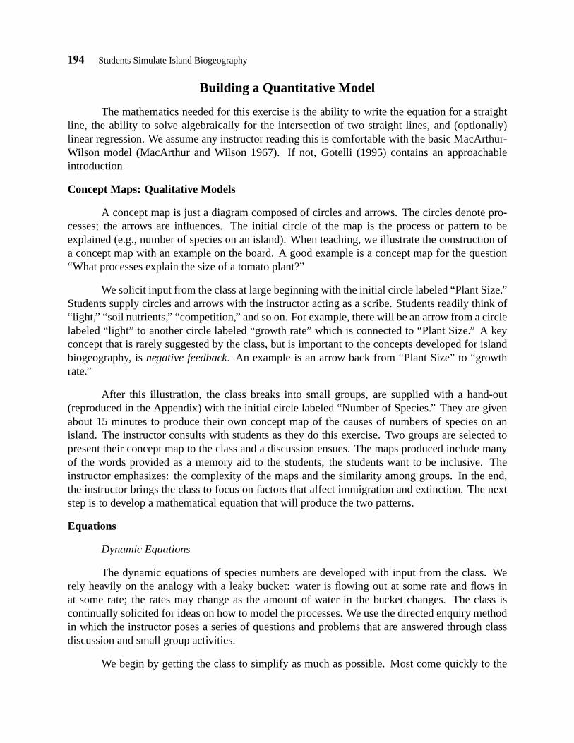
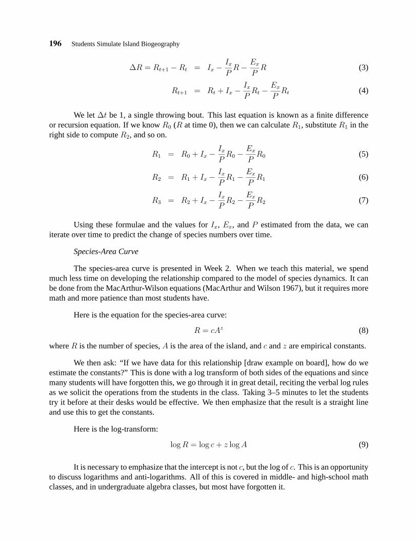
idea that competition controls extinction rates. We ask for a hypothesized graphical relationshipbetween extinction and competition (What is on the y axis? What is on the x axis? Does it increaseor decrease? Is it straight or curved? Which is simpler?) We ask how to quantify this vague ideaof competition. Many students will volunteer amount of food, number of individuals. Stressingthat simplification is critical, the class is brought to the idea thatspecies numbersis a reasonablesurrogate for degree of competition. They are then asked to graph the effect species number onextinction rate as an x-y graph. The instructor draws the axes and asks for input on the axes labelsand the qualitative relationship (linear with positive slope). This is repeated for the effects ofspecies number on the rate of immigration ofnew species to the island. With increasing speciesnumbers, immigration decreases linearly from a maximum rate to 0 when the number of specieson the island is equal to the number on the mainland (and therefore no new species can possiblyarrive). Figure 1 shows the relationships. Before writing the equations in the form shown, we askthe class for the equation. Everyone knowsy = mx + b for extinction. The negative slope takesmore thought for some and we get them to suggesty = q − rx. We do not introduce the notationof Fig. 1 until later.

Ix

R P(# species)

xxI=I /P)R−(I

Imm

igra

tion

(I)

Ex

R (# species) P

Ext

inct

ion

FIGURE 1: The basic hypotheses of the effect of species number on immigration and extinction rates.R isnumber of species on the island.P is the number of species in the pool (e.g., on the mainland).Ix andEx

are constants: maximum immigration and extinction rates, respectively.

Here is the equation for species dynamics:

dR

dt= NR = Ix −

Ix

PR︸︷︷︸

Immigration

− Ex

PR︸︷︷︸

Extinction

(1)

whereR is numbers of species, NR is the “Net Rate of change of numbers of species” (NR isactuallydR/dt, but we try not to scare away too many, even though many have had calculus),Ix

is the maximum immigration rate (whenR = 0), P is the number of species on the mainland,Ex

is the maximum extinction rate (whenR = P ).

Most students do not recognize the derivative form of the equation, so we convert it into adifference equation so that we can generate the dynamics of species numbers. We usually do notattempt this until Week 2. Here is how to do it:

NR =dR

dt≈ ∆R

∆t= Ix −

Ix

PR− Ex

PR (2)


∆R = Rt+1 −Rt = Ix −Ix

PR− Ex

PR (3)

Rt+1 = Rt + Ix −Ix

PRt −

Ex

PRt (4)

We let∆t be 1, a single throwing bout. This last equation is known as a finite differenceor recursion equation. If we knowR0 (R at time 0), then we can calculateR1, substituteR1 in theright side to computeR2, and so on.

R1 = R0 + Ix −Ix

PR0 −

Ex

PR0 (5)

R2 = R1 + Ix −Ix

PR1 −

Ex

PR1 (6)

R3 = R2 + Ix −Ix

PR2 −

Ex

PR2 (7)

Using these formulae and the values forIx, Ex, andP estimated from the data, we caniterate over time to predict the change of species numbers over time.

Species-Area Curve

The species-area curve is presented in Week 2. When we teach this material, we spendmuch less time on developing the relationship compared to the model of species dynamics. It canbe done from the MacArthur-Wilson equations (MacArthur and Wilson 1967), but it requires moremath and more patience than most students have.

Here is the equation for the species-area curve:

R = cAz (8)

whereR is the number of species,A is the area of the island, andc andz are empirical constants.

We then ask: “If we have data for this relationship [draw example on board], how do weestimate the constants?” This is done with a log transform of both sides of the equations and sincemany students will have forgotten this, we go through it in great detail, reciting the verbal log rulesas we solicit the operations from the students in the class. Taking 3–5 minutes to let the studentstry it before at their desks would be effective. We then emphasize that the result is a straight lineand use this to get the constants.

Here is the log-transform:

log R = log c + z log A (9)

It is necessary to emphasize that the intercept is notc, but the log ofc. This is an opportunityto discuss logarithms and anti-logarithms. All of this is covered in middle- and high-school mathclasses, and in undergraduate algebra classes, but most have forgotten it.


Logistics of Student Simulation of Colonization Rates

After the linear relationships between species number and extinction and immigration rateis hypothesized, we introduce the students to the experimental system (string and petrie plates)with which they are going to act out the colonization and extinction process. The students areassigned to groups (3 is optimal) and we then go outside.

Materials

Each group of 3 or 4 students will need the following:

1. A countdown timer or stopwatch to time the throwing (“colonization”) bouts

2. Loops of string to simulate square islands

3. 4 stakes (e.g., large nails) for the corners of the island (masking tape for carpet if indoors)

4. One container of labeled plastic petri dishes (20 “species”, 10 individuals per species). Their colormarkings or numbers distinguish species. This is the mainland or “source population” box.

5. 1 clipboard with 3 or 4 data sheets (1 data sheet for each simulation)

6. A meter stick or tape

7. A grassy (or carpeted) area at least 5 m away from other groups

Student Logistics

1. We have successfully done the exercise outside on a grass lawn and inside on a low-napcarpet. Each group should have either 4 or, preferrably, 3 students.

2. For each group, you will need an area about 6m by 8m, to prevent interaction among groups.

3. Each mainland species pool should have 20 species and 10 individuals per species. Moreindividuals would probably be better, but there are cost and convenience issues. Individualsare standard plastic petri dishes, where each half is used as an individual. Each individualis marked with its species identification. We denote species using 2 methods: 10 speciesare numbered on white tape 1 through 10 for 10 species. The other 10 species are givencolored tape codes: single lengths of tape about 2 inches long and two pieces of tape in across pattern (e.g., a length of blue tape and a length of black tape). This doesn’t seem toconfuse the students, but better labels would be all 20 species as upper-case letters of thealphabet on white tape. We store the mainland pool in plastic garbage bags.

4. Islands are loops of string stretched tautly into squares and affixed to the substrate at thecorners. When outside, we use large nails as anchors; masking tape works well on carpet.Students are given the string for the islands already cut to length and knotted to remove onemore confusing activity during the exercise.

5. The student hand-out indicates that the students should simulate 2 distances (2m and 4m)and 2 island sizes (1 m2 and 0.25 m2). In a 3 hour lab period, with all the group activities


and directed enquiry interaction, in Week 1 there is time only for 1 island size (1 m2) and 2distances (2 m and 4 m).

In Week 2, we test the species-area curve and distance on small islands. One group ofstudents do small islands (0.25 m2) at 2 and 4 m. Other groups do 2 replicates of 1 island4 m from the mainland with sizes 0.09, 0.49, 0.81, and 2.0 m2. These plus 0.25 and 1.0 m2

gives 6 areas for estimating the constants of the species-area curve.

6. Here is the order of events during the simulation:

(a) Setup: The students collect their materials and set up the first experiment: (1) Identifya spot for the thrower (i.e., the mainland); (2) using a meter stick, measure the distancebeing simulated from the mainland to either the edge or center of the island; (3) selectthe appropriate loop of string for the island area; (4) determine which student will be thethrower, scorer, andtimer/recorder; (5) deposit all of the colonizing individuals withineasy reach of the thrower at the mainland; (6) (Important!) Randomize the individualsin the mainland by mixing the pile well.

(b) Simulation: (1) The timer signals to the thrower to begin, (2) the thrower grabs anindividual from the mainland and sails it towards the island (those Frisbee skills arefinally useful); (3) the thrower repeats this as rapidly as possible for 15 seconds; (4)after a 15 sec throwing bout, the scorer and recorder examine the island: they firstidentify and remove all extinctindividuals and those that overlap the string by lessthan one-half their diameter; (5) the scorer reports to the recorder which species arepresent and the recorder marks those species on the appropriate line of the data sheet;(6) while this is occurring, the thrower returns the non-colonizing individuals to themainland pile and re-mixes the pile, (7) the next throwing bout proceeds while therecorder calculates and records the number of immigrations and extinctions, and theresultant number of species on the island for the previous bout. See the hand-out at theend that gives a worked example.

(c) Scoring: (1) an individual is killed when another individual lands on top of it; (2) anindividual fails to colonize if less than 1/2 of its diameter is outside the square; (3) aspecies does not go extinct until the last individual of its species is killed.

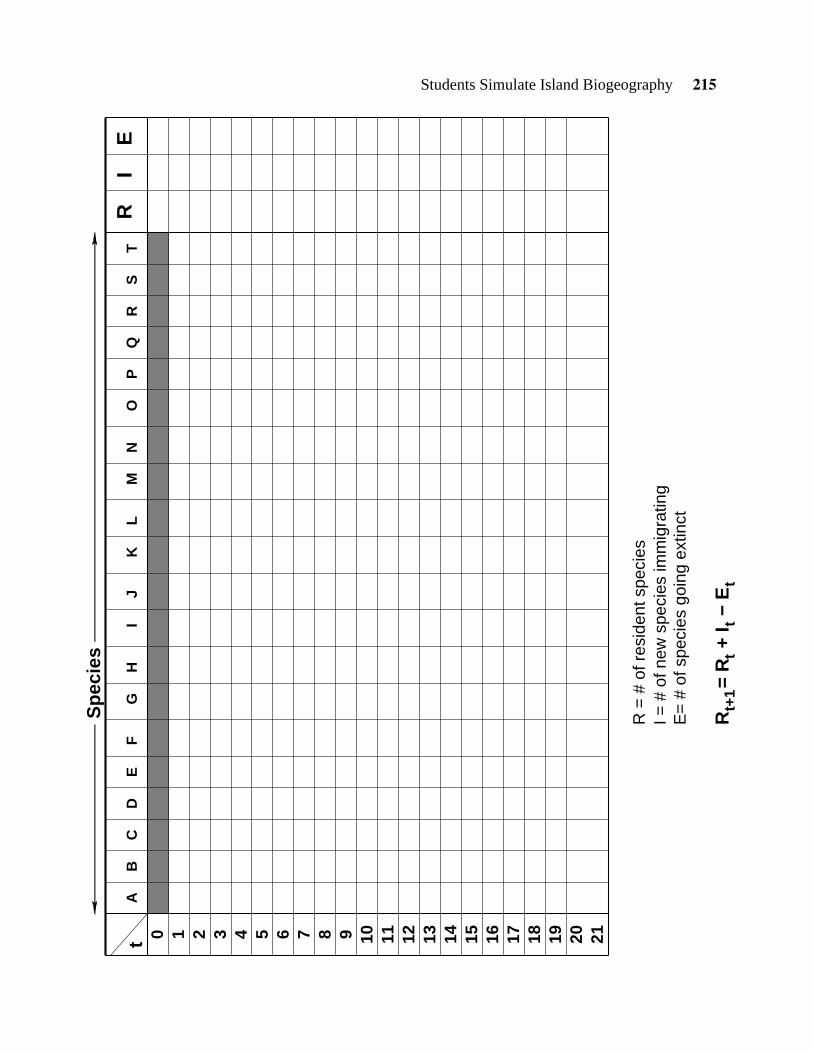
(d) Recording: (1) students record only presence or absence of a species by putting an“X” in the appropriate position in the data sheet; numbers of individuals are not used;(2) immigration rate: count the number of “X”s that were not present in the earlierthrowing bout (line above current line of data sheet); record this number in the “I”column of theline above the current data sheet line; (3) extinction rate: count thenumber of data sheet cells (species) that do not have an “X” in the current line but didhave one in the line above; record this number in the “E” column of theline above thecurrent data sheet line; (4) number of species: from the line above the current datasheet line add “R” plus “I” minus “E” and record it in the “R” column of thecurrentdata sheet line.


The data sheets follow at the end of this document in the Appendix.

Logistics of Student Simulation of Species-Area Curve

The layout and organization of students is the same as above. Convenient areas to add to the0.25 m2 and 1.0 m2 areas already done above are: 0.09, 0.49, 0.81, and 2.0 m2. Assign one groupto each area. Since the purpose of this exercise is only to get estimates of the equation parametersc andz, we do not need to estimate extinction and immigration rates. Each group should colonizeas above, but after each bout, records only the number of species on the island. When the numbersare approximately contant over three consecutive bouts, the group can stop the simulation.

Sharing Data and Data Analysis

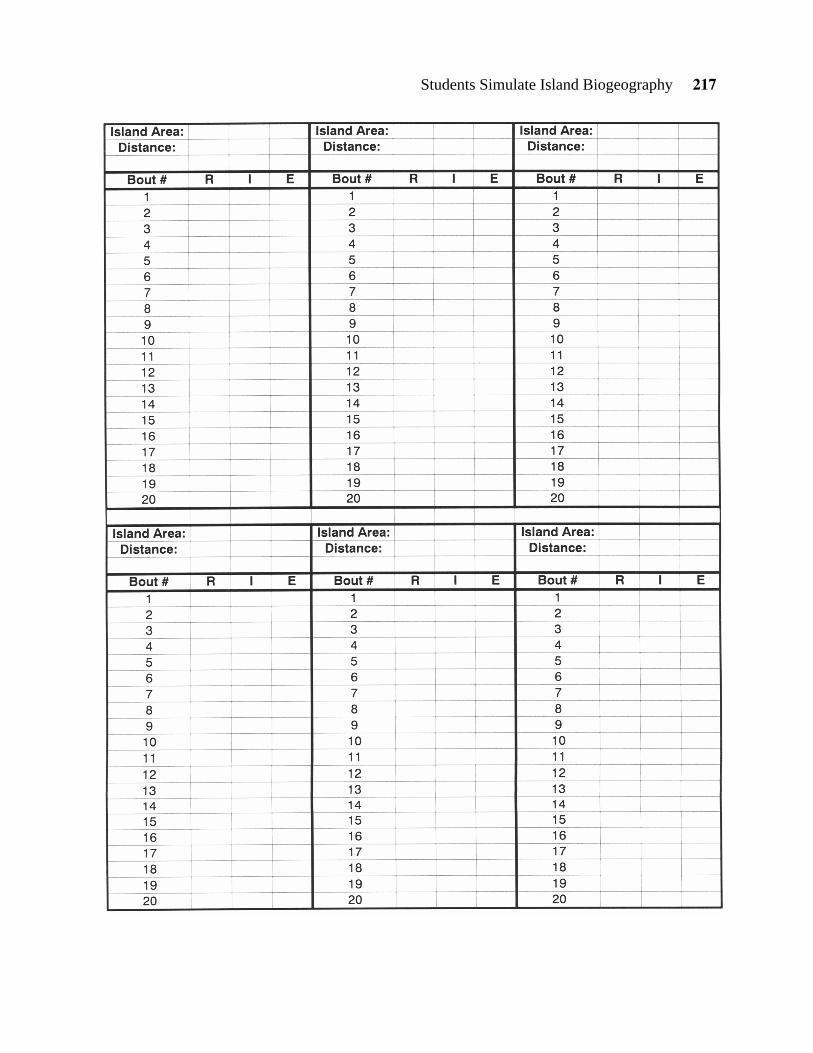
After the simulation, students return to the classroom and write their values ofR, Ix andEx

on the board. All students copy the numbers on the summary data sheets provided in the Appendix.

After Week 1 (see homework below): Students should plot the data and estimate the con-stants in the model. With these, they can solve for the equilibrium number of species.

After Week 2 (see homework): The students can iterate the recursion equation to get specieschange. They should also analyze their area data by plottingR versusA, by taking the log of bothsides of the species-area equation and plottinglog R versuslog A.

There is an interesting discrepancy between real island extinction and that simulated here.In the petri plate world, individuals are killed only by new immigrants. In the real world, death dueto competition produces starvation or physiological stress, most commonly by resident individu-als. The result of this discrepancy is that in the petri plate world, extinctions are correlated withimmigrations and any variable that changes immigration will also change extinction. In particular,distance affects immigration rates, so in our simulations it will also affect extinction rates. Theusual (simple) presentation of island biogeography theory assumes distance affects only immigra-tion and island size affects only extinction rates. In petri plate world, it is possible (and has beenobserved in our classes) that far islands will have more species than near islands because as dis-tance decreases extinction rate is increased more than immigration rate is increased. This is worthworking out on the board for the students.

Practice Problems

To prepare the students for the homework that is distributed at the end of Week 2, we spendabout 30 minutes doing practice problems after completing the species-area simulation. In theclassroom, we hand-out the problems without the solutions. We ask the students to help solve theproblems as a group. Below are some examples that we use. Some of the problems benefit bybreaking the students into small groups to give them some time to solve the problems. After allthe problems have been discussed, we hand-out the solutions and the homework for the followingweek.


Example Practice Problem Set

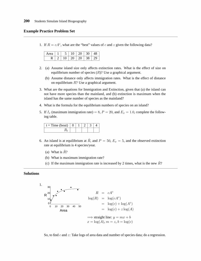
1. If R = cAz, what are the “best” values ofc andz given the following data?

Area 1 5 10 20 30 48R 2 10 20 20 38 29

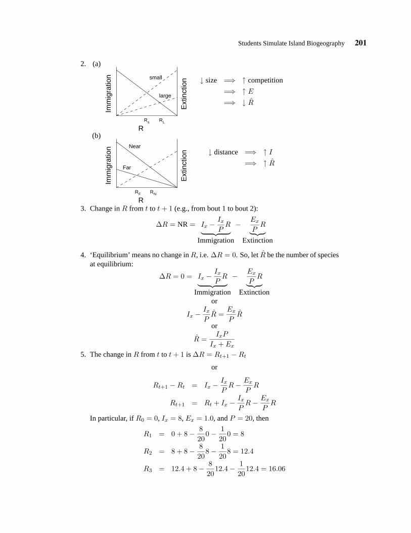
2. (a) Assume island size only affects extinction rates. What is the effect of size onequilibrium number of species (R)? Use a graphical argument.

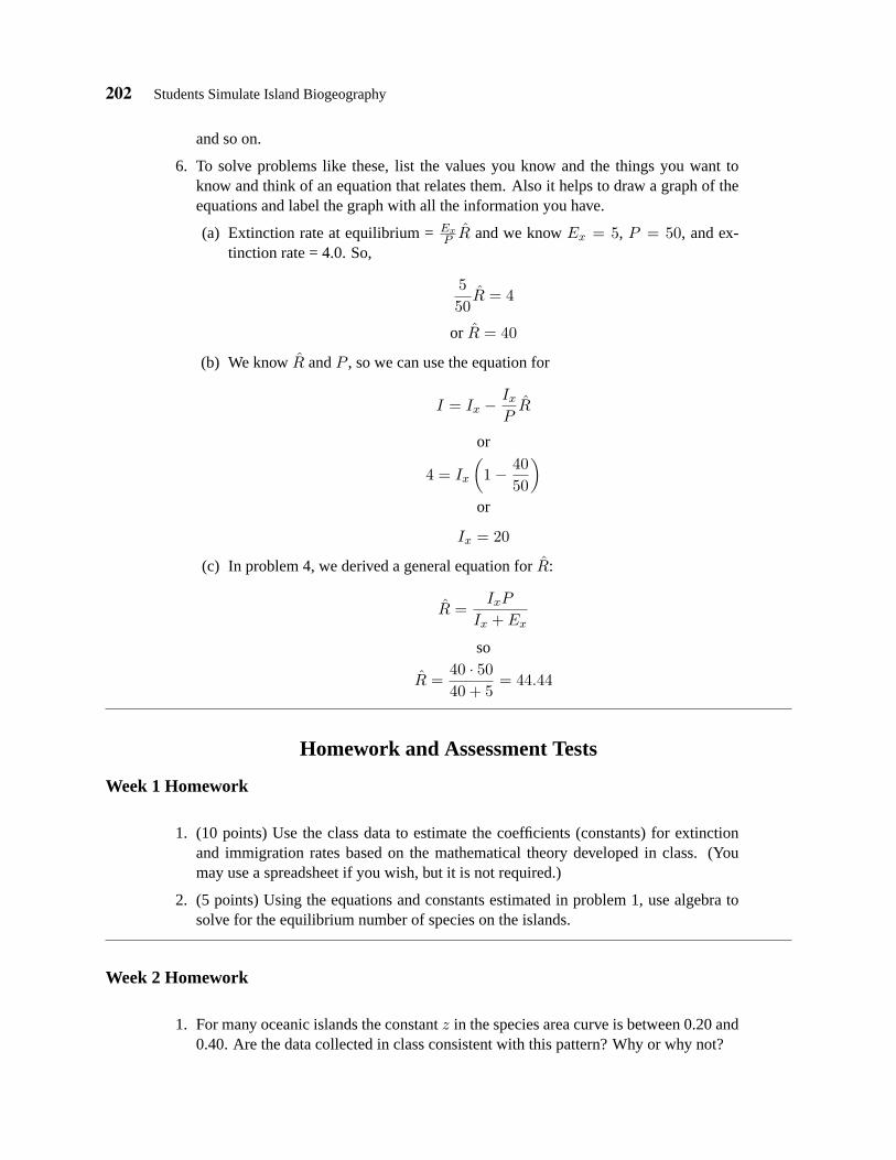
(b) Assume distance only affects immigration rates. What is the effect of distanceon equilibriumR? Use a graphical argument.

3. What are the equations for Immigration and Extinction, given that (a) the island cannot have more species than the mainland, and (b) extinction is maximum when theisland has the same number of species as the mainland?

4. What is the formula for the equilibrium numbers of species on an island?

5. If Ix (maximum immigration rate)= 8, P = 20, andEx = 1.0, complete the follow-ing table.

t = Time (bout) 0 1 2 3 4Rt

6. An island is at equilibrium at̂R, andP = 50, Ex = 5, and the observed extinctionrate at equilibrium is 4 species/year.

(a) What isR̂?

(b) What is maximum immigration rate?

(c) If the maximum immigration rate is increased by 2 times, what is the newR̂?

Solutions

1.

R

010 20 30 40 50

30

20

10

0

Area

R = cAz

log(R) = log(cAz)= log(c) + log(Az)= log(c) + z log(A)

=⇒ straight line:y = mx + bx = log(A), m = z, b = log(c)

So, to findc andz: Take logs of area data and number of species data; do a regression.


2. (a)

R

small

large

Rs RL

Imm

igra

tion

Ext

inct

ion ↓ size =⇒ ↑ competition

=⇒ ↑ E

=⇒ ↓ R̂

(b)

R

Imm

igra

tion

Ext

inct

ion

RF RN

Near

Far

↓ distance =⇒ ↑ I

=⇒ ↑ R̂

3. Change inR from t to t + 1 (e.g., from bout 1 to bout 2):

∆R = NR = Ix −Ix

PR︸︷︷︸

Immigration

− Ex

PR︸︷︷︸

Extinction

4. ‘Equilibrium’ means no change inR, i.e. ∆R = 0. So, letR̂ be the number of speciesat equilibrium:

∆R = 0 = Ix −Ix

PR︸︷︷︸

Immigration

− Ex

PR︸︷︷︸

Extinctionor

Ix −Ix

PR̂ =

Ex

PR̂

or

R̂ =IxP

Ix + Ex

5. The change inR from t to t + 1 is ∆R = Rt+1 −Rt

or

Rt+1 −Rt = Ix −Ix

PR− Ex

PR

Rt+1 = Rt + Ix −Ix

PR− Ex

PR

In particular, ifR0 = 0, Ix = 8, Ex = 1.0, andP = 20, then

R1 = 0 + 8− 820

0− 120

0 = 8

R2 = 8 + 8− 820

8− 120

8 = 12.4

R3 = 12.4 + 8− 820

12.4− 120

12.4 = 16.06


and so on.

6. To solve problems like these, list the values you know and the things you want toknow and think of an equation that relates them. Also it helps to draw a graph of theequations and label the graph with all the information you have.

(a) Extinction rate at equilibrium =ExP R̂ and we knowEx = 5, P = 50, and ex-

tinction rate = 4.0. So,

550

R̂ = 4

or R̂ = 40

(b) We knowR̂ andP , so we can use the equation for

I = Ix −Ix

PR̂

or

4 = Ix

(1− 40

50

)or

Ix = 20

(c) In problem 4, we derived a general equation forR̂:

R̂ =IxP

Ix + Ex

so

R̂ =40 · 5040 + 5

= 44.44

Homework and Assessment Tests

Week 1 Homework

1. (10 points) Use the class data to estimate the coefficients (constants) for extinctionand immigration rates based on the mathematical theory developed in class. (Youmay use a spreadsheet if you wish, but it is not required.)

2. (5 points) Using the equations and constants estimated in problem 1, use algebra tosolve for the equilibrium number of species on the islands.

Week 2 Homework

1. For many oceanic islands the constantz in the species area curve is between 0.20 and0.40. Are the data collected in class consistent with this pattern? Why or why not?


2. Regressions of immigration rates and extinction rates against species numbers gavethese equations.

I = 7.8− 0.55R

E = 0.12R

What is the equilibrium number of species?

3. How many species will on the island described in problem 2 foreachof the first 5colonization bouts?

4. In the table below are values of amphibians and reptiles on West Indian islands. (Val-ues are logarithms of square kilometers and species numbers.)

log10 Area 0.415 1.30 2.06 4.02 4.11 5.11 5.32log10 Number of Species 0.602 0.845 0.954 1.61 1.59 1.95 1.93

(a) What are the constants of the species-area curve?

(b) Plot the number of species versus area using an arithmetic scale (not a logarith-mic scale).

5. In many cases, isolated patches of habitat within a continent act like islands for theorganisms that require that habitat. Forest fragmentation and the reduction of habitatdue to human activities (e.g., urban sprawl, logging, etc) is causing the decline ofmany populations, ultimately resulting in their local extinction in the affected areas.You are a manager of a forest preserve that is scheduled to have its area reduced by0.5 due to a new housing development. Based on the following, how many species doyou expect will exist in the preserve after the development?

Assume: (a) the number of species on the preserve is constant, but there are annualextinctions and arrivals of new species, (b) the number of species in the area surround-ing the threatened preserve that could colonize is 50, (c) the maximum immigrationrate to the preserve is 8 species per year, (d) before development, the preserve lost 2species per year, and (e) if the area is reduced by 0.5, the extinction rate doubles.

Solutions to Week 2 Homework

1. Take the logarithms of area: 0.09, 0.25, 0.49, 0.81, 1.0, and 2.0 and of the corre-sponding species numbers. Regresslog(R) vs log(A) statistically or by “eye.” Theregression coefficients will give you the parameters:z is the slope, andc is 10 raisedto the power of the intercept (if you used log base 10).

2. At equilibrium:

I = E =⇒ 7.8− 0.55R̂ = 0.12R̂

=⇒ R̂ = 7.8/0.67 = 11.64=⇒ R̂ = 11 since species are integers)

3. I = immigration rate,E = extinction rate

Rt+1 = Rt + I − E


= Rt + 7.8− 0.55Rt − 0.12Rt = Rt + 7.8−).67Rt

or

R0 = 0R1 = 0.0 + 7.8− (0.67)(0.0) = 7.8R2 = 7.8 + 7.8− (0.67)(7.8) = 10.374R3 = 10.374 + 7.8− (0.67)(10.374) = 11.22R4 = 11.22 + 7.8− (0.67)(11.22) = 11.503R5 = 11.503 + 7.8− (0.67)(11.503) = 11.596

4. After taking logarithms and doing linear regression:z = 0.28248 andc = 100.4532 =2.839.

5. Ex = maximum extinction rate,Ix = maximum immigration rate.

GIVEN: P = 50 andI = 8=⇒ I = 8− 8/50R = 8− 0.16R

GIVEN: E = 2 at equilibrium

=⇒ 8− 0.16R̂ = 2=⇒ R̂ = 37.66=⇒ E atR̂ = 2 = (Ex/P )R̂ = (Ex/50)(37.66)=⇒ Ex = 2.655

GIVEN: Decrease area by 1/2

=⇒ Ex = 2.0Ex,old

=⇒ at new equilibrium:I = E =⇒ 8− 0.16R̂ = (2)(0.0531)R̂=⇒ R̂ = 30.05 ≈ 30

Example Pre-test

Pre-tests and post-tests are very good things to do. It not only gives the instructor essentialfeedback, but we have found that class averages do generally improve by about 15–20% in theseskills. This can be useful ammunition when students complain to your superiors that the course istoo difficult. In addition to testing for quantitative skills using the following math questions, wealso request information about the student’s previous math and biology courses including gradesearned (omitted here). It is very revealing to correlate grades in calculus and performance on thepre-tests.

Assessment 1: Do NOT write your name.1. Here are two equations:

y1 = 3.0x

y2 = 10.0− x


(a) Using the axes below, label the axes with numbers and graph the two lines.

(b) Use algebra (not the graph) and find the value ofx wherey1 equalsy2. Showyour work.

2. Below are data on the kilocalories required by birds of different sizes to fly 1 km.

You want to statistically fit these data to the following equation:

y = axb

(a) Describe in words how you would obtain the best estimates ofa andb. Showany algebra manipulations you would do.

(b) Without using a calculator, circle one of the following that you think is true:b > 1 b = 1 0 < b < 1 b = 0 b < 0.

3. Suppose we have a disease with these properties: Every year, the disease increasesby N new cases, and every year a fixed proportion (c) of the diseased cases (D) arecured. Answer the following:

(a) Write an equation for the rate of change of the disease:

∆D =

(b) Over time, which of the following is true: (a) the disease will increase foreverwithout bound, (b) the disease will go to extinction, or (c) the disease will leveloff at constant numbers. Use graphs to explain why you chose the answer youdid.

Example Post-test

Assessment 2: Do NOT write your name.1. Here are two equations:

y1 = 1.0y2 = 2.0− 0.4x

(a) Using the axes below, label the axes with numbers and graph the two lines.

(b) Use algebra (not the graph) and find the value ofx wherey1 intersectsy2. Showyour work.

2. Below are data relating heart rate (R) and body mass (M ) for several species of ver-tebrates.

You want to statistically fit these data to the following equation:

R = aM b

(a) Describe in words how you would obtain the best estimates fora andb. Showany algebra manipulations you would do.

(b) Without using a calculator, circle one of the following that you think is true:b > 1 b = 1 0 < b < 1 b = 0 b < 0.

3. In the steamy jungles of South America, there lives a bird of great beauty: the exoticResplendent Whoopee. Each year a constant (D) number of birds die. The number ofnew Whoopees born in a given year decreases from a maximum (M ) linearly as thenumber of adult Whoopees (W ) increases.

Answer the following:

(a) Write an equation for the rate of change of the Whoopee numbers:

∆W =

(b) Over time, which of the following is true: (a) the Whoopee will increase foreverwithout bound, (b) the Whoopee will go to extinction, or (c) the Whoopee willlevel off at constant numbers. Use graphs to explain why you chose the answeryou did.

Typical Results from Students

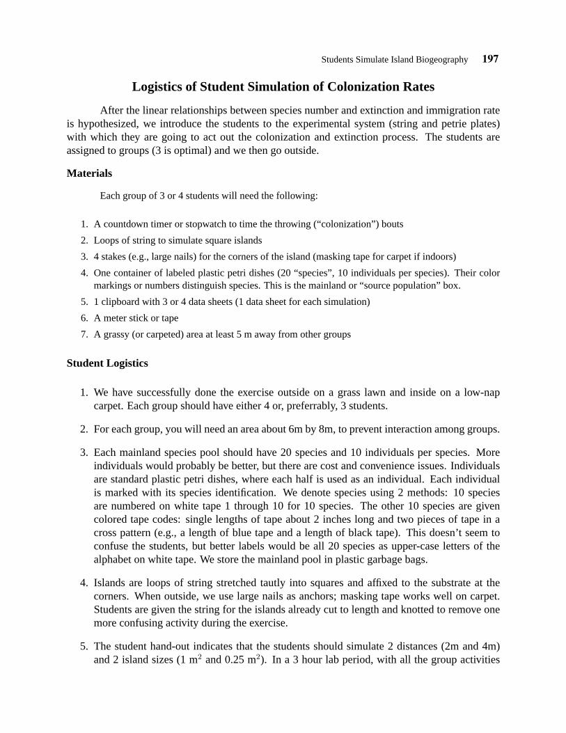
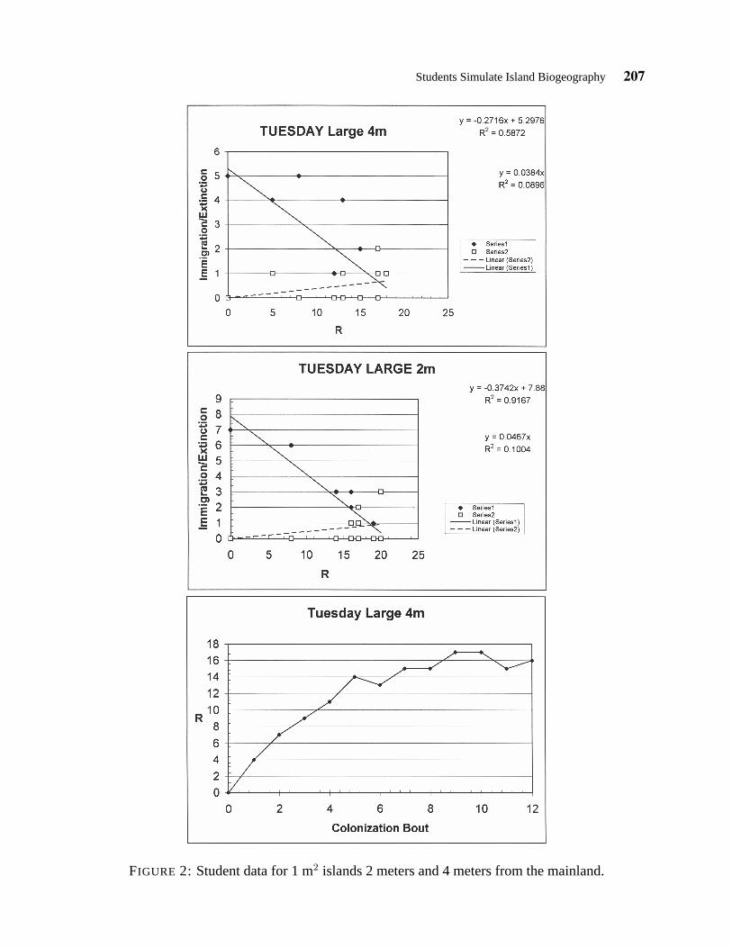
Figure 2 show typical results from the simulated colonization experiments. As can be seen,there is ample opportunity for discussing the nature of statistical variation both within and betweenstudent groups.

Improvements

The extinction rates are really too low. This can be increased with a rule like: “Individualsare killed if a new colonist falls within 3 cm.” But this would be difficult to implement withoutdirect touching of the disks.



FIGURE 2: Student data for 1 m2 islands 2 meters and 4 meters from the mainland.


Student Guide to Simulating Island Biogeography

Laboratory Goals

Understand the use of mathematics in the scientific method as it applies to formulating andtesting the theory of island biogeography.

Laboratory Objectives

1. Identify key variables determining the number of species on an “island.”

2. Qualitatively explain how key variables determine the number of species on an “island.”

3. Demonstrate mathematically how key variables determine the number of species on an “is-land” and the equilibrium species richness.

4. Design a quantitative experiment that synthesizes the key variables that determine the num-ber of species on an “island.”

5. Statistically compare experimental data with theoretical predictions.

Materials

Each group of 3 or 4 students will need the following:

1. A countdown timer or stopwatch to time the “colonization” bouts

2. Loops of string to simulate square islands

3. 4 stakes for the corners of the island (masking tape for carpet if indoors)

4. One container of labeled plastic petri dishes (20 “species”, 10 individuals per species). Theircolor markings or numbers distinguish species. This is the mainland or “source” population.

5. 1 clipboard with 3 or 4 data sheets (1 data sheet for each simulation)

6. A meter stick or tape to measure island distances and sizes

7. A grassy (or carpeted) area at least 5 m away from other groups

Experimental Protocol

Creating Your Islands

1. Determine what your group’s square island dimensions and distance from the source popu-lation will be. It will be one of the following:

Close (2m) Far (4m)Small (0.25 m2) X XLarge (1.0 m2) X X


2. With the meter stick, string, and stakes or tape, locate your island anywhere safe on theplaying field. For example, you do not want your flight path intersecting with another group’sflight path.

3. Establish your source population (i.e., the container with all the petri dishes). To do this,measure your group’s island distance from the center of your island in any safe direction.Plant a flag or stake at this location. This is where you will be dispersing your species. Sit orkneel with the container containing your source population (the one with all the petri dishes)at this spot.

Division of Labor

Each group consists of 3 or 4 students. The following jobs need to be distributed amonggroup members.

1. Thrower: This person should be your most precise and unbiased thrower (i.e., consistentlyaccurate). Practice to determine this. The thrower tosses as many plastic discs from thesource population box, while sitting or kneeling, as he or she can in 15 seconds. The throwermay not throw the next disc until the previously thrown disc has hit the ground. You mayfind it convenient to put the “immigrating” species in a pile in front of you.

2. Timer/Scorer: The time keeps track of the three replicates of 20, 15-second colonizationevents. The timer shouts start and stop to disc thrower at the beginning and end of a colo-nization event.The scorer examines the island and calls out to Recorder the identity of the resident species(R) after each 15-second colonization event. The scorer also returns unsuccessful colonists(discs outside the island) to the mainland area after each 15 second round. Be sure to mix thesource population discs after each round to maintain an approximately random distribution.

3. Recorder: This person records on the data sheets the species present after a throwing boutas determined by the scorer. Furthermore, he or she keeps track of immigration (I) andextinction (E) events. All information is tallied on the data sheets provided (one sheet perreplicate experiment of 20, 15 second bouts).

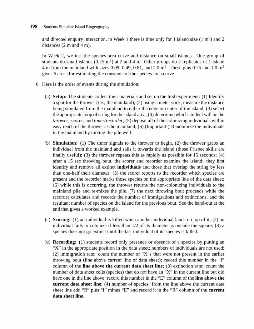
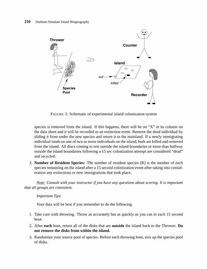
Figure 3 depicts the relationships of the three team members.

Scoring Definitions and Rules

After a colonization bout, the number of immigrants and extinctions are tallied. See thehand-out that illustrates how to score immigrations and extinctions.

1. Immigrant (I): An immigration event is the arrival on the island of an individual (disk)which was not present in the prior colonization bout. At least one-half of the disc must beinside the boundary to count as a successful individual.

2. Extinctions (E) and Individual Deaths: An individual dies and is removed from the islandif another individual lands on top of it. A species goes extinct when the last individual in its


PoolSpecies

killed

Recorder

Counter

out

Island

Thrower

FIGURE 3: Schematic of experimental island colonization system

species is removed from the island. If this happens, there will be no “X” in its column onthe data sheet and it will be recorded as an extinction event. Remove the dead individual bysliding it from under the new species and return it to the mainland. If a newly immigratingindividual lands on one of two or more individuals on the island, both are killed and removedfrom the island. All discs coming to rest outside the island boundaries or more than halfwayoutside the island boundaries following a 15 sec colonization attempt are considered “dead”and recycled.

3. Number of Resident Species:The number of resident species (R) is the number of eachspecies remaining on the island after a 15 second colonization event after taking into consid-eration any extinctions or new immigrations that took place.

Note:Consult with your instructor if you have any questions about scoring. It is importantthat all groups are consistent.

Important Tips

Your data will be best if you remember to do the following.

1. Take care with throwing. Throw as accurately but as quickly as you can in each 15 secondbout.

2. After eachbout, return all of the disks that areoutside the island back to the Thrower.Donot remove the disks from within the island.

3. Randomize your source pool of species. Before each throwing bout, mix up the species poolof disks.


Tallying Data

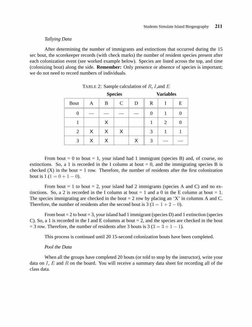
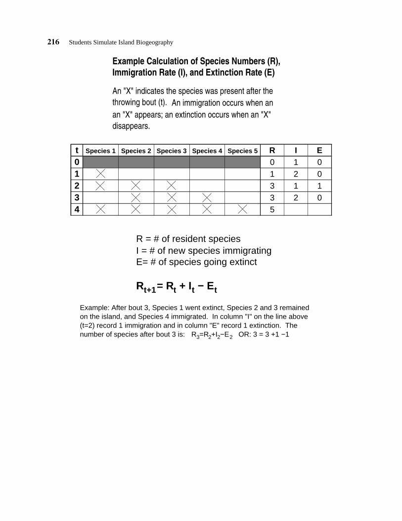
After determining the number of immigrants and extinctions that occurred during the 15sec bout, the scorekeeper records (with check marks) the number of resident species present aftereach colonization event (see worked example below). Species are listed across the top, and time(colonizing bout) along the side.Remember: Only presence or absence of species is important;we do not need to record numbers of individuals.

TABLE 2: Sample calculation ofR, I,andE

Species Variables

Bout A B C D R I E

0 — — — — 0 1 0

1 X 1 2 0

2 X X X 3 1 1

3 X X X 3 — —

From bout = 0 to bout = 1, your island had 1 immigrant (species B) and, of course, noextinctions. So, a 1 is recorded in the I column at bout = 0, and the immigrating species B ischecked (X) in the bout = 1 row. Therefore, the number of residents after the first colonizationbout is 1 (1 = 0 + 1− 0).

From bout = 1 to bout = 2, your island had 2 immigrants (species A and C) and no ex-tinctions. So, a 2 is recorded in the I column at bout = 1 and a 0 in the E column at bout = 1.The species immigrating are checked in the bout = 2 row by placing an ‘X’ in columns A and C.Therefore, the number of residents after the second bout is 3 (3 = 1 + 2− 0).

From bout = 2 to bout = 3, your island had 1 immigrant (species D) and 1 extinction (speciesC). So, a 1 is recorded in the I and E columns at bout = 2, and the species are checked in the bout= 3 row. Therefore, the number of residents after 3 bouts is 3 (3 = 3 + 1− 1).

This process is continued until 20 15-second colonization bouts have been completed.

Pool the Data

When all the groups have completed 20 bouts (or told to stop by the instructor), write yourdata onI, E andR on the board. You will receive a summary data sheet for recording all of theclass data.


Species-Area Curve

To estimate the parameters of the species-area curve, we need more than two areas. Someof the groups, as assigned by the instructor, will also simulate colonization at four other areas.The activities are exactly as before,exceptyou do not need to record numerically immigrationsand extinctions. Here, we are interested only in the equilibrium number of species. So, after eachcolonizing bout, kill the individuals that overlap, return the outside plates to the thrower, and recordthe number of species on the island. Repeat until the numbers of species is approximately constantover three bouts. Record the final number of species and pool your results with the other groups.

Acknowledgements

This laboratory exercise in mathematical modeling in biology was developed with fundingfrom the U.S. Department of Education program Fund to Improve Post-Secondary Education toUtah State University: P116B971688.

Literature Cited

Begon, M., J. L. Harper, and C. R. Townsend. 1990.Ecology: Individuals, Populations, Commu-nities.Blackwell Scientific Publications. Boston, MA.

Cangelosi, J. S. 1996.Teaching Mathematics in Secondary and Middle School: An InteractiveApproach.Second Edition. Prentice Hall, Englewood Cliffs, NJ.

Gotelli, N. J. 1995.A Primer of Ecology.Sinauer Associates, Inc. Sunderland, MA.

MacArthur, R. H. and E. O. Wilson. 1967.The Theory of Island Biogeography.Princeton Univer-sity Press, Princeton, NJ.

Simberloff, D. S. and E. O. Wilson. 1969. Experimental zoogeography of islands: the colonizationof empty islands. Ecology 50:278–296.

Appendices: Data Sheets

The following data sheets are included.

1. Template for the Concept Map exercise.2. Datasheet for student simulation of colonization: original version.3. Datasheet for student simulation of colonization: New version using alphabet letters for

species names4. Example calculation ofR, I, andE5. Datasheet for class pooled colonization data6. Datasheet for class pooled Species-Area curve data


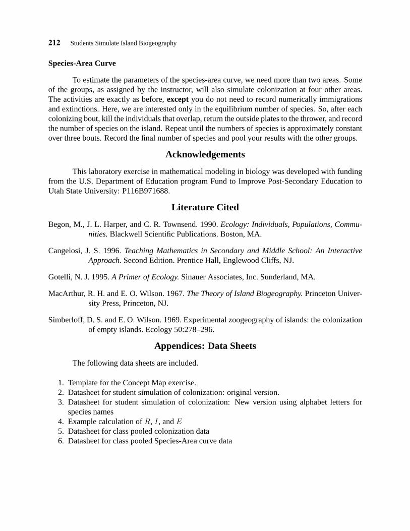
CONCEPT MAP FOR BIOGEOGRAPHY:POSSIBLE ECOLOGICAL CONCEPTS(Use ONLY the concepts you think are REALLY important.)

POP GROWTH RATE PREDATION MUTUALISMK SELECTION ABIOTIC ENV. DISPERSALPHYSIOLOGICAL TOLERANCE FITNESS ALLOMETRYPARAPATRY ISLAND SIZE SYNERGISMCOMPETITION EVOLUTION NUTRIENT CYCLINGSUCCESSION NICHE SPECIES DIVERSITYDENSITY DEPENDENCE CONSUMPTION ENERGY FLOWCOOPERATION PRIMARY PRODUCTIVITY PLATE TECTONICSMAINLAND DISTANCE AGGRESSION RESOURCE LEVELSCOOPERATION CARRYING CAPACITY GENETIC DIVERSITYEFFICIENCY POP. CYCLES DEMOGRAPHY

Number of specieson an island


12

34

56

78

910

RI

Mas

kP

ink

Pin

kM

ask

0 2 3 5 6 7 8 9 10 11 12 13 15 16 17 18 19 20 21141 4

Bla

ckB

lue−

EB

lack

Yel

low

Gre

enW

hit

eB

lue

t

Rt+

1=

Rt +

I t −

Et

Sp

ecie

s

R =

# o

f res

iden

t spe

cies

I = #

of n

ew s

peci

es im

mig

ratin

gE

= #

of s

peci

es g

oing

ext

inct


AB

CD

EF

GH

IJ

KL

MN

OP

QR

ST

RI

0 2 3 5 6 7 8 9 10 11 12 13 15 16 17 18 19 20 21141 4

Et

Rt+

1=

Rt +

I t −

Et

Sp

ecie

s

R =

# o

f res

iden

t spe

cies

I = #

of n

ew s

peci

es im

mig

ratin

gE

= #

of s

peci

es g

oing

ext

inct


R

Immigration Rate (I), and Extinction Rate (E)Example Calculation of Species Numbers (R),

throwing bout (t).an "X" appears; an extinction occurs when an "X"disappears.

An "X" indicates the species was present after the An immigration occurs when an

Example: After bout 3, Species 1 went extinct, Species 2 and 3 remainedon the island, and Species 4 immigrated. In column "I" on the line above(t=2) record 1 immigration and in column "E" record 1 extinction. The

3 2+I2−E2 OR: 3 = 3 +1 −1number of species after bout 3 is: =R

t012

43

Species 1 Species 2 Species 3 Species 4 Species 5 R I E01335

2121 0

010

Rt+1= Rt + It − Et

R = # of resident speciesI = # of new species immigratingE= # of species going extinct



ISLAND AREA NUMBER OF SPECIES

(square meters)

Date post:	02-May-2017
Category:	Documents
Upload:	christerop
View:	221 times
Download:	2 times

IslandBiogeography Students Colonize Islands to Test Hypotheses 12-Haefner

Documents