Graph-Theoretic Algorithms for the“Isomorphism of Polynomials” Problem

Charles Bouillaguet, Pierre-Alain Fouque and Amandine Veber

1 Universite de Lille-1 charles.bouillaguet@univ-lille1.fr2 Universite de Rennes-1

pierre-alain.fouque@univ-rennes1.fr3 CMAP Lab, CNRS and Ecole Polytechnique

amandine.veber@cmap.polytechnique.fr

Abstract. We give three new algorithms to solve the “isomorphism of polynomial” problem, which wasunderlying the hardness of recovering the secret-key in some multivariate trapdoor one-way functions. Inthis problem, the adversary is given two quadratic functions, with the promise that they are equal upto linear changes of coordinates. Her objective is to compute these changes of coordinates, a task whichis known to be harder than Graph-Isomorphism. Our new algorithm build on previous work in a novelway. Exploiting the birthday paradox, we break instances of the problem in time q2n/3 (rigorously) andqn/2 (heuristically), where qn is the time needed to invert the quadratic trapdoor function by exhaustivesearch. These results are obtained by turning the algebraic problem into a combinatorial one, namely thatof recovering partial information on an isomorphism between two exponentially large graphs. These graphs,derived from the quadratic functions, are new tools in multivariate cryptanalysis.

1 Introduction

The notion of equivalent linear maps is a basic concept in linear algebra; two linear functions f and gover vector spaces are equivalent if and only if there exist two other linear bijective functions S andT such that f = T ◦ g ◦ S. Geometrically speaking, this means that f and g are essentially the samefunction, but with coordinates expressed in different bases. The computational problem consisting intesting the equivalence of two linear functions (given by matrices) is easy, because it is well-knownthat two linear maps are equivalent if and only if they have the same rank.Computing the rank itselfcan be done in polynomial time, and is usually efficient.

This notion of equivalent linear maps lends itself to an obvious generalization, by dropping therequirement that the functions shall be linear. Then, given two vector spaces U and V , of respectivedimension n andm, two functions f, g : U → V are said to be equivalent if there exist an invertible n×nmatrix S and an invertible m×m matrix T such that g = T ◦f ◦S. Again, the geometric interpretationof this notion is that g and f are “the same function”, up to linear changes of coordinates. However,deciding the equivalence of two functions is no longer easy in general.

The case where f and g are polynomial maps is particularly relevant, not only because it is anatural generalization of the linear case, but also because f and g admit a compact representation. Itis understood that a polynomial map f is such that each coordinate of the vector f(x) is a polynomialexpression of the coordinates of the vector x. Testing the equivalence of two polynomial maps hasbeen called the “Isomorphism of Polynomials” (IP) problem by Patarin in 1996 [43], and later the“Polynomial Linear Equivalence” (PLE) problem by Faugere et al. in 2006 [25].

One aspect of PLE that makes it a bit difficult to study is that depending on the parameters(dimensions and base field of the vector spaces, degree of the polynomials, special restrictions, etc.),the problem can take very different forms. We will thus focus on the case where the base field ofthe vector space is finite (of size q), where polynomials are quadratic, and where their domain andcodomain are the same, i.e., where f, g : (Fq)

n → (Fq)n are quadratic maps. This is the setting that

appears in most cryptographic constructions. In the sequel we will call this particular restriction the

Quadratic Maps Linear Equivalence (QMLE) problem. In order to make our exposition simpler, we willfurthermore assume that q, the size of the finite field, is a power of two. The theory of quadratic formspresents itself very differently for odd characteristic and for characteristic two, and in order not toexpose two variants of each of our results, we chose the most computer-oriented setting.

The first “multivariate” cryptographic schemes relied on a somewhat heuristic construction to buildTrapdoor One-Way Functions, whose security was based on the hardness of QMLE. Starting with aneasy-to-invert quadratic map f , one builds an apparently random-looking one by setting g = T ◦f ◦S.The idea is that the changes of coordinate would hide the structure of f that makes it easy to invert, sothat g would look random. Inverting random quadratic maps is extremely hard, and the best optionsin general are exhaustive search (if q is small), or the computation of a Groebner basis (when q islarge), both techniques being exponential in n. This construction backed one of the advertized goalsof multivariate cryptography, namely the ability to encrypt or sign n-bit blocks while offering n bitsof security, as opposed to, e.g. RSA.

In this setting, g (and eventually f) is the public key, while S and T are the secret key. Whenf is public, then recovering the secret-key precisely means solving an instance of QMLE. Severalcryptosystems have been built on this idea [10, 55, 18, 32, 15, 7], but they have all been broken [29,24, 20, 19, 37, 29, 35, 9, 28, 40, 11]. The main reason behind this fiasco is that the specific instances ofQMLE exposed by these schemes were weak because f was too special, so that polynomial-time and/orefficient algorithms to crack them have eventually been designed.

In a different direction, Patarin also proposed to use the hardness of arbitrarily chosen instances ofthe PLE problem to design a public-key identification scheme, thus potentially avoiding the aforemen-tioned disaster. A prover, who has generated a pair of private/public keys (PK,SK), wants to proveher identity to a verifier who knows PK. In fact the prover aims to convince that she knows SK, butwithout revealing any information about SK to the verifier, or to anybody else. In 1986, Goldreich,Micali and Wigderson [33] built an elegant zero-knowledge proof system for Graph Isomorphism (GI)and used it to build an identification scheme. There, PK is a pair of isomorphic graphs, and SK isthe isomorphism (a permutation of the vertices). In order for this system to be secure, it must be hardto solve the instance of GI formed by the public-key. Despite a large research effort, until now no algo-rithm has been able to solve instances of GI in worst-case polynomial, which is certainly encouraging.However, most instances of GI, and in particular random instances, are extremely easy to solve. Thus,the identification scheme of [33] relied on a presumably hard problem for which we do not know howto generate non-trivial instances...

Patarin’s suggestion was that Graph Isomorphism could be replaced by QMLE, with the hope thatrandom instances of the problem would then be hard, and that key-generation would then be straight-forward. There was apparently nothing to lose with the new problem, because it was shown to beharder than GI [44]. Using random instances would in principle avoid the weak instances that hadbeen broken. The resulting QMLE-based identification scheme is not particularly efficient, and doesnot enjoy very attractive key-sizes, but it is quite simple. It also has a few interesting features com-pared to other identification schemes based on NP-hard combinatorial problems such as [47–52]: mostnotably, it does not require hash functions nor commitment schemes, and it does not require the partiesto share a (usually large) public common string describing an instance of the NP-complete problem.

1.1 Related Work

The QMLE problem is reminiscent of the Even-Mansour cipher [23], which turns a fixed n-bit permuta-tion P into an n-bit block-cipher with 2n-bit key by setting Ek1,k2(x) = P (x+k1)+k2. Attacks againstthis construction aim to recover the keys while only having black-box access to E and P . One of itsdistinctive features is that the performance of a successful adversary running in time t and sending qqueries is limited by t · q ≥ 2n, under the assumption that P is a random permutation. The known

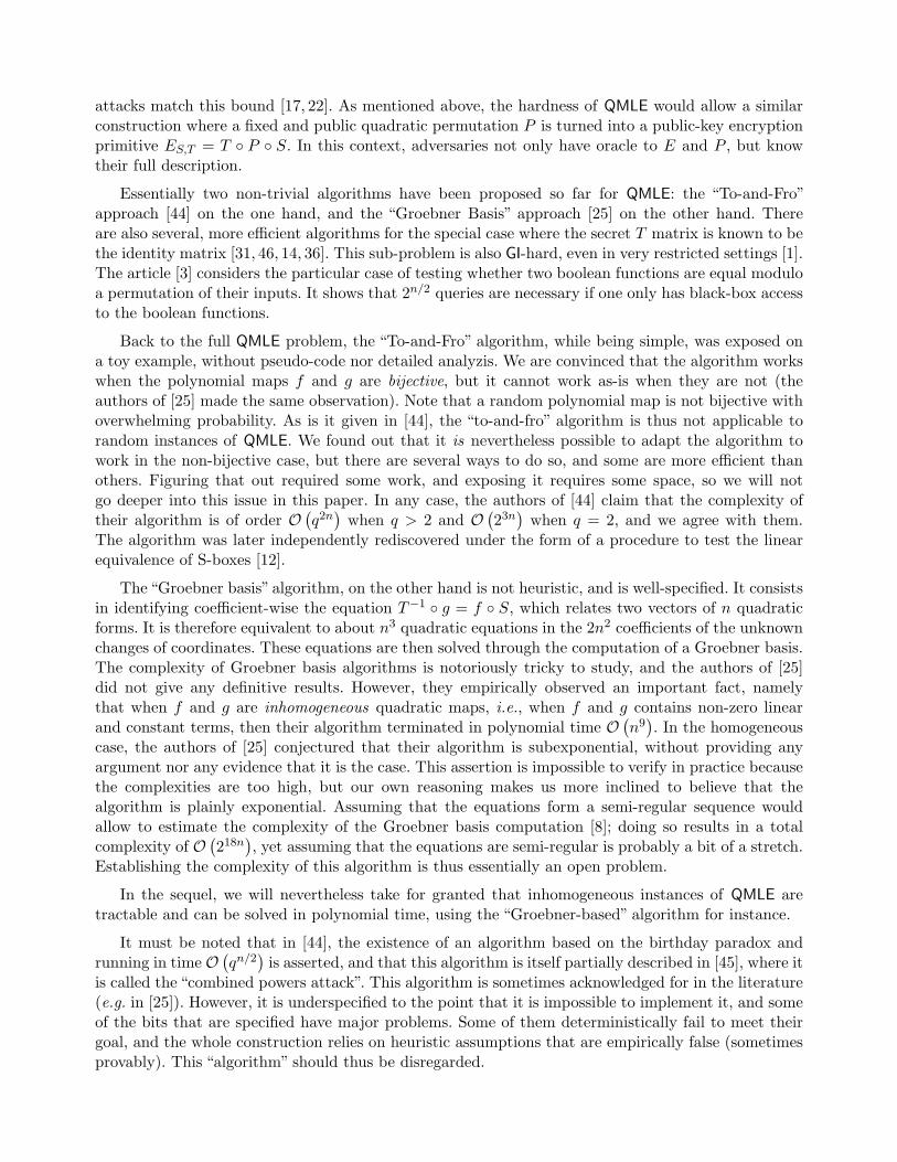
attacks match this bound [17, 22]. As mentioned above, the hardness of QMLE would allow a similarconstruction where a fixed and public quadratic permutation P is turned into a public-key encryptionprimitive ES,T = T ◦ P ◦ S. In this context, adversaries not only have oracle to E and P , but knowtheir full description.

Essentially two non-trivial algorithms have been proposed so far for QMLE: the “To-and-Fro”approach [44] on the one hand, and the “Groebner Basis” approach [25] on the other hand. Thereare also several, more efficient algorithms for the special case where the secret T matrix is known to bethe identity matrix [31, 46, 14, 36]. This sub-problem is also GI-hard, even in very restricted settings [1].The article [3] considers the particular case of testing whether two boolean functions are equal moduloa permutation of their inputs. It shows that 2n/2 queries are necessary if one only has black-box accessto the boolean functions.

Back to the full QMLE problem, the “To-and-Fro” algorithm, while being simple, was exposed ona toy example, without pseudo-code nor detailed analyzis. We are convinced that the algorithm workswhen the polynomial maps f and g are bijective, but it cannot work as-is when they are not (theauthors of [25] made the same observation). Note that a random polynomial map is not bijective withoverwhelming probability. As is it given in [44], the “to-and-fro” algorithm is thus not applicable torandom instances of QMLE. We found out that it is nevertheless possible to adapt the algorithm towork in the non-bijective case, but there are several ways to do so, and some are more efficient thanothers. Figuring that out required some work, and exposing it requires some space, so we will notgo deeper into this issue in this paper. In any case, the authors of [44] claim that the complexity oftheir algorithm is of order O

(q2n)

when q > 2 and O(23n)

when q = 2, and we agree with them.The algorithm was later independently rediscovered under the form of a procedure to test the linearequivalence of S-boxes [12].

The“Groebner basis” algorithm, on the other hand is not heuristic, and is well-specified. It consistsin identifying coefficient-wise the equation T−1 ◦ g = f ◦ S, which relates two vectors of n quadraticforms. It is therefore equivalent to about n3 quadratic equations in the 2n2 coefficients of the unknownchanges of coordinates. These equations are then solved through the computation of a Groebner basis.The complexity of Groebner basis algorithms is notoriously tricky to study, and the authors of [25]did not give any definitive results. However, they empirically observed an important fact, namelythat when f and g are inhomogeneous quadratic maps, i.e., when f and g contains non-zero linearand constant terms, then their algorithm terminated in polynomial time O

(n9). In the homogeneous

case, the authors of [25] conjectured that their algorithm is subexponential, without providing anyargument nor any evidence that it is the case. This assertion is impossible to verify in practice becausethe complexities are too high, but our own reasoning makes us more inclined to believe that thealgorithm is plainly exponential. Assuming that the equations form a semi-regular sequence wouldallow to estimate the complexity of the Groebner basis computation [8]; doing so results in a totalcomplexity of O

(218n

), yet assuming that the equations are semi-regular is probably a bit of a stretch.

Establishing the complexity of this algorithm is thus essentially an open problem.

In the sequel, we will nevertheless take for granted that inhomogeneous instances of QMLE aretractable and can be solved in polynomial time, using the “Groebner-based” algorithm for instance.

It must be noted that in [44], the existence of an algorithm based on the birthday paradox andrunning in time O

(qn/2

)is asserted, and that this algorithm is itself partially described in [45], where it

is called the “combined powers attack”. This algorithm is sometimes acknowledged for in the literature(e.g. in [25]). However, it is underspecified to the point that it is impossible to implement it, and someof the bits that are specified have major problems. Some of them deterministically fail to meet theirgoal, and the whole construction relies on heuristic assumptions that are empirically false (sometimesprovably). This “algorithm” should thus be disregarded.

1.2 Our Results

We give three algorithms to solve QMLE in the homogeneous case. All these algorithms work by re-ducing the solution of a homogeneous (hard) instance into that of one or several inhomogeneous (easy)instances after some preprocessing. We will thus assume that we are given a (black-box) Inhomogeneoussolver that presumably works in polynomial time, and we will count the number of inhomogeneousqueries sent to this oracle. We are well-aware that this assumption is quite strong. The empiricalsuccess of the algorithm of [25] convinced us that it works in polynomial-time on average, yet movingfrom there to “worst-case polynomial time” seems like a leap of faith. However, this assumption easesour exposition considerably, and in practice there does not seem to be any problem (probably becausethe queries sent to the inhomogeneous oracle are random enough).

Our three algorithms differ by the number of queries they send to the oracle, by the amount ofcomputation they perform themselves, and by their success probability.

Algo. Section Preprocessing Inhom. queries success prob.1 x qn 12 y O

(n3 · q2n/3

)q2n/3 62%

3 z O(n5 · qn/2

)1 62 % only when q = 2

Algorithm 1 is deterministic, and essentially performs an exhaustive search in (Fq)n, sending one

inhomogeneous query per vector. Using the algorithm of [25] to deal with the inhomogeneous instances,the resulting complexity is O

(n9 · qn

), which already improves on the “to-and-fro” algorithm of [44].

Algorithms 2 and 3 rely on the birthday paradox to improve on exhaustive search and break theqn barrier. To this end, two exponentially large isomorphic graphs are derived from the two quadraticmaps. Recovering a bit of information on an isomorphism allows to make the problem inhomogeneous,and thus easy to solve. The trick is that this partial information must be extracted without knowing thefull graphs, because they are too large. The construction of these graphs borrows from the differentialtechniques that have broken SFLASH, amongst others.

Algorithm 2 is relatively easy to analyze and we rigorously establish its complexity and successprobability when dealing with random instances of the problem. Algorithm 3 is more efficient butmore sophisticated and harder to analyze (as well as somewhat heuristic). We provide an as-rigorous-as-possible complexity analysis under a conjecture on random quadratic maps, and we verify experi-mentally that we are not off by too much.

Because our algorithms are exponential in n, we do not fully break Patarin’s identification scheme(it is of no practical value anyway), even though its key-sizes should in principle be doubled. Theconstruction of a Trapdoor One-Way Function from QMLE outlined above has already been bludgeonedto death by cryptanalysts, and it now lies on the autopsy table. We take the role of the medical examinerthat appears in every good police drama, only to discover that the corpse had cancer even beforebeing brutally assaulted. We indeed believe that our algorithms condemn this generic construction ofa Trapdoor One-Way Function post-mortem, and give a theoretical reason not to try again, besides theobvious “they have all been broken” argument. Our algorithms indeed break the QMLE instance andretrieve the secret-key (asymptotically) much faster than inverting the quadratic map by exhaustivesearch. This shows in passing that this construction can only offer n/2 bits of security, instead of then that was its original objective.

2 A First Algorithm Based on Dehomogenization

Confronted with a homogeneous instance of QMLE, our strategy throughout this paper is to build aninhomogeneous instance admitting the exact same solutions. This inhomogeneous instance can in turnbe solved in polynomial time, and reveals the solution(s) of the original problem. The downside of this

approach is that the image of S must be known at one arbitrary point of the vector space. Indeed, ifβ = S · α, then:

∀x. g(x) = T · f(S · x) ⇐⇒ ∀x. g(x+ α) = T · f(S · x+ β).

Thus defining g′(x) = g(x+ α) and f ′ = f(x+ β) yields an equivalent problem, i.e., an instance thathas the same solutions as the original one. In addition, the new instance is inhomogeneous. This followsfrom the simple observation that although x2 is a homogeneous polynomial, (x+ α)2 = x2 + αx+ α2

is not since it has a non-trivial linear term αx and a non-trivial constant term α2.It follows that solving (homogeneous) instances of QMLE essentially boils down to finding Sα, for

some known and non-zero vector α. Exhaustive search is the first option that comes to mind, leadingto Algorithm 1. This algorithm sends qn queries to the inhomogeneous solver in the worst case, andfinds the solutions when they exist. This algorithm terminates with probability one in time O

(n9 · qn

)if the Groebner-based algorithm of [25] is used to solve the inhomogeneous instances. Despite beingextremely simple, Algorithm 1 is asymptotically qn times faster than to the “to-and-fro” algorithmof [44].

Algorithm 1 Simple algorithm based on dehomogenization.function Exhaustive-Dehomogenization(f, g)

x← random non-zero vector in (Fq)n

for all 0 = y ∈ (Fq)n do

f ′(z)← f(z + y)g′(z)← g(z + x)query IQMLE-Solver with (f ′, g′′)if solution (S, T ) found then return (S, T )

return “Not Equivalent”

This dehomogenization technique exposes a crucial asymmetry in the problem: it is apparentlymuch more critical to obtain knowledge on S than on T . This is not new: the “To-and-Fro” algorithmrelies on the ability to transfer knowledge of a relation β = S · α to a relation g(α) = T · f(β).

3 Moving the Problem Into a Graphic World

Using the birthday paradox is a natural idea to improve on exhaustive search algorithms in manyscenarii, with the hope to halve the exponent in the complexity. Here, we wish to use the birthdayparadox to obtain the image of S at one point, and build a dehomogenized instance, just as we didin the previous section. One difficulty is that we want to focus only on S, and leave T alone. To thisend, we introduce a tool which is, to the best of our knowledge, new. We associate a graph Gh to anyquadratic map h : (Fq)

n 7→ (Fq)n. Its vertices are the elements of (Fq)

n, and there is an edge betweenx, y ∈ (Fq)

n if and only if h(x+ y) = h(x) + h(y). To some extent, Gh expresses the “linear behavior”of h (even though h is not linear) and thus we call these graphs the “linearity graphs” of the associatedquadratic maps.

These graphs are natural objects associated to quadratic maps. For instance, the distinguisherof [21] to determine whether a given quadratic map f is an HFE public key can be rephrased asfollows: pick a random node in Gf , and count its neighbors. If their number exceeds a given bound(which depends on the degree of the internal HFE polynomial), then return “random”, else return“HFE”. With the right bound on the number of neighbors, this algorithm achieves subexponentialadvantage.

The essential interest of linearity graphs for our purposes is that the two graphs Gf and Gg areconnected by the secret matrix S.

Lemma 1. If T ◦ g = f ◦ S then S is a graph isomorphism that sends Gf to Gg.

Proof. Indeed, if x↔ y in Gg, then by definition g(x+y) = g(x)+g(y), and it follows that T ◦g(x+y) =T ◦g(x)+T ◦g(y), and thus that f(S ·x+S ·y) = f(S ·x)+f(S ·y). This in turn means that S ·x↔ S ·yin Gf . It follows that S is a graph isomorphism between Gf and Gg.

Linearity graphs thus allows a formulation of the problem where the other secret matrix T is nolonger present. We have two (exponentially large) isomorphic graphs Gf and Gg, and we ultimatelyneed to recover the whole isomorphism S. However, thanks to the dehomogenization technique of theprevious section, and thanks to the ease with which inhomogeneous instances can be solved, it turnsout that recovering just a little bit of information on the isomorphism is enough to find it completely.More precisely, we just need to know how the isomorphism S transforms one arbitrary vertex.

Of course, completely building these graphs is prohibitively expensive (they have qn vertices). Itturns out that this is never necessary, because it is possible to walk in these graphs without fullyknowing them.

Walking in Linearity Graphs. The function ψ(x, y) = f(x + y) + f(x) + f(y) is a generalizationof the polar form of a quadratic form to vectors thereof, in characteristic two. It is easy to check thatψ is bilinear. Given a (non-zero) vertex x ∈ (Fq)

n in the graph, the function:

Dxf : y 7→ ψ(x, y) = f(x+ y) + f(x) + f(y)

is a familiar object in multivariate cryptology, called the Differential of f at x [27, 21, 19, 29]. It is alinear function from (Fq)

n to (Fq)n, which is then conveniently represented by a matrix. The set of

nodes adjacent to x in Gf is in fact the kernel of Dxf . Note that x always belong to kerDxf , becausex + x = 0. The main reason we chose to focus on the case where q = 2e is that this fact is not truewhen q is not a power of two.

The matrix Dxf is easy to compute given f and x. If f is a (homogeneous) quadratic map, then it isin fact a vector of n quadratic forms, which can conveniently be described by a collection of n matricesF1, . . . , Fn, that are interpreted as follows: Fk[i, j] is the coefficient of xixj in the k-th component off . If tM denotes the transpose of M , then the matrix representation of the differential of f at x isgiven by:

Dxf =

x · (F1 + tF1) . . . x · (Fn + tFn)

.

Thus, given a vector x, finding the neighbors of x in Gf can be done in time O(n3): computing

the matrix Dxf requires n matrix-vector products, and determining its kernel classically takes O(n3)

operations. It is thus possible to crawl the linearity graphs by spending a polynomial number ofelementary operations on each traversed vertex.

Structure in Linearity Graphs. Linearity graphs possess a rich structure, thanks to their algebraicorigin. Recall that in Gf , two nodes x and y are adjacent if ψ(x, y) = 0, where ψ is the symmetricbilinear map defined above. The bilinearity of ψ induces a lot of structure in Gf . For instance, wealways have ψ(x, x) = 0, and by bilinearity ψ(λx, µx) = λµψ(x, x) = 0, so that the q multiples of avector x form a clique in Gf . The set of all multiples of x are thus topologically indifferentiable (theyall have the exact same neighborhood).

Furthermore, the same reasoning shows that if two vectors x and y are adjacent in Gf , then theset of q2 linear combinations λx+ µy form a clique in Gf of size q2.

Degree Distribution. If a quadratic map f is randomly chosen (amongst the finite number ofpossibilities), then the resulting linearity graph Gf follows a certain —mostly unknown— probabilitydistribution, and any property of Gf can be seen as a random variable. One of the most interestingproperties of Gf is the distribution of the degree (i.e., of the number of neighbors) of vertices in Gf .This result is stated in terms of the probability that a random n× n matrix over Fq is invertible. Wedenote it by λ(n):

λ(n) =n∏

i=1

(1 − 1

qi

)

Lemma 2 (theorem 2 in [21]). Let x ∈ (Fq)n be a non-zero vector, and f : (Fq)

n → (Fq)n be a

uniformly random quadratic map. Then Dxf is a uniformly random matrix vanishing over x. As aconsequence, the probability that Dxf has a kernel of dimension k ≥ 1 is:

λ(n)λ(n− 1)λ(k)λ(k − 1)λ(n− k)

q−k(k−1)

Because λ(n) is a decreasing function of n that converges to a finite limit bounded away from zero,then the ratio of the λ-expressions lives in a small interval, independently of q, n and k, so that theprobability is in fact of order q−k(k−1). Of course, over Fq, a k-dimensional vector space contains qk

elements, so that if dim kerDxf = k, then the vertex x has qk neighbors.

Sparsity. Computing the expectation and the variance of the degree is technical, but feasible:

E [degree] = q − 1qn−2

σ2 = q2(q − 1)(

1 − q2 + 1qn

+q2

q2n

)Establishing these two expressions is somewhat technical, yet because both are sums of q-hypergeometricterms, they can be computed by “creative telescoping” thanks to the q-analog of Zeilberger’s algo-rithm [56]4. It follows that the expected number of edges of Gf is essentially qn+1/2. In other terms,Gf is a very sparse graph that has barely more edges than it has vertices.

Disconnecting Linearity Graphs. A linearity graph Gf is fully connected, because all vertices areadjacent to the “zero” vertex. This “zero” vertex is not very interesting (since it is adjacent to everyother vertex), and, as a matter of fact, it even turns out to be a bit annoying. Thus, it seems thatthere is nothing to lose by removing it. In addition, we could also get rif of the self-loops ; they areuseless since every vertex has one.

We thus denote by G∗f the simple graph Gf in which the zero vertex has been removed, and where

self-edges are removed. It is interesting to note that the resulting graph is no longer connected, andthat there are in fact very many connected components. Indeed, if dim kerDxf = 1, then the onlyneighbors of x are its multiples, and x belong to a connected component of size q − 1. Lemma 2 tellsus that this happens with probability λ(n)/λ(1), and this converges to a finite limit bounded awayfrom zero when n goes to infinity. Thus, a constant fraction of the vertices belong to “small” connectedcomponents of size q − 1. Working a bit on the λ functions reveals that this proportion grows like1 − 1/q2.

4 The conscientious reviewer will find this derivation in Appendix A.

4 Count Your Neighbors: A Simple Graph-and-Birthday Algorithm

It is well-know that if two graphs (V1, E1) and (V2, E2) are isomorphic, and if ρ is an isomorphismbetween them, then u ∈ V1 and ρ(u) ∈ V2 have the same degree, i.e., the same number of neighbors.It follows that if u ∈ V1 and v ∈ V2 do not have the same degree, then they cannot be related by ρ.

We adapt this simple idea in the context of QMLE, under the form of Algorithm 2. The main ideain this algorithm is to target vertices in the linearity graphs of f and g that have a specific degree:we only look for a “right pair” y = S · x amongst vertices x, y that have a prescribed degree (chosento optimise the complexity of the algorithm). The remaining of this section is devoted to establishingthe properties of this algorithm, which are summarized in the following theorem.

Algorithm 2 First Birthday Based Algorithm1: function SampleSet(h)2: L← ∅3: repeat4: repeat5: x← random vertex of Gh

6: until x has q√

n/3 neighbors7: L← L ∪ {x}8: until |L| =

√2qn/3

9: return L

10: function Neighbor-Counting-QMLE(f, g)11: U ← SampleSet (f)12: V ← SampleSet (g)13: for all (x, y) ∈ U × V do14: f ′(z)← f(z + y)15: g′(z)← g(z + x)16: query IQMLE-Solver with (f ′, g′)17: if solution (S, T ) found then return (S, T )

18: return “Probably not equivalent”

Theorem 1. Algorithm 2 performs O(q2n/3

)units of computations on average, sends at most q2n/3

queries to the inhomogeneous solver, and succeeds with probability 1 − 1/e.

The helper function SampleSet returns a set of O(qn/3

)vertices of Gf (resp. Gg), each having

q√

n/3 neighbors in the graph. It follows that there are q2n/3 queries to the inhomogeneous solver,because this is the size of the cartesian product U × V .

It remains to establish the complexity of SampleSet, and the success probability of the algorithm.As explained above, since we are looking for a “right pair” y = S · x, it is safe to restrict our attentionto vertices x, y that have a specific degree (as long as vertices with such a degree exist in the graphs).

Lemma 2 gives us the expected number iterations of the innermost loop of SampleSet that arerequired to find a random vertex with the required degree. Up to a constant factor, finding a vertexwith degree qk requires qk(k−1) trials, so that finding each new random vertex requires O

(qn/3

)rank

computations on n× n matrices, hence O(n3 · qn/3

)operations.

Lemma 2 also tells us that there are on average qn−k(k−1) vertices in Gf each having degree qk. In

Algorithm 2 we look specifically at vertices of degree q√

n/3, and we thus expect Gf to contain q2n/3

of them. Since the number of iterations of the outermost repeat...until loop is roughly the squareroot of this number, we do not expect more than a constant number of “extra” iterations finding an

already-known vector x. Putting everything together, we conclude that SampleSet terminates afterO(n3q2n/3

)operations.

Now, the birthday bound tells us that U×V contains a“right pair”y = Sx with probability greaterthan 63%, because both U and V contain about the square root of the total number of vertices withdegree q

√n/3 (see [53] for a precise statement of this specific version of the birthday paradox).

Practical Results. We have implemented Algorithm 2 inside the MAGMA computer algebra sys-tem[13], running on one core of a 2.8 Ghz Xeon machine. As shown in Table 1, we found out that inpractice it is difficult to balance the cost of building U and V on the one hand, and going throughthe candidate pair on the other hand, because the target degree can only take

√n integer values. We

could nevertheless verify in practice that the complexity of building the lists and the expected numberof right pairs in them is consistent with our expectations. The source code is in the public domain,and is available on the webpage of the first author. It uses an unpublished algorithm to solve theinhomogeneous instances.

n q generating U and V total time logq (target degree) |U | # pairs

16 2 0s 68s 3 1 4

22 2 28s 9h45m 4 13 400

28 2 4913s 2h15m 5 8 64

Table 1. Experimental results on Algorithm 2.

5 Map Your Neighborhood: A Faster Graph-And-Birthday Algorithm

We have seen in section 3 that the linearity graphs, once deprived from the“zero”vertex, contain manysmall connected components. Of course, if y = Sx, then the connected component of x is isomorphicto the connected component of y. In this section, we describe an algorithm that builds upon thisidea—instead of just looking at immediate neighbors, as we did in algorithm 2, we now try to look atthe whole connected component, in order to distinguish between vertices of the same degree.

Canonical Graph Labeling. Given a graph G, a Canonical Labeling algorithm relabels the ver-tices of G, thus producing a graph Canon(G), which is by definition isomorphic to G. The result iscanonical in the sense that if G and H are isomorphic graphs, then Canon(G) = Canon(H). Thecanonical labels are therefore complete invariants of the isomorphism class, and as such, computinga canonical labeling is necessarily harder than checking if two graphs are isomorphic. However, com-puting a canonical labeling can be done in average linear time [6], because except for an exponentiallysmall fraction of all graphs, it can be done with a very simple linear algorithm. Deterministic algo-rithms that always succeed are subexponential, with complexity O

(exp

(√n log n

))[5]. The perhaps

most well-known, and most practical algorithm dates back to 1978, and is implemented in the nautyopen-source package [38]. It is known to be exponential on some specific counter-examples [39], butotherwise performs exceptionally well. There are also many relevant classes of graphs where canon-ical labeling is polynomial [26]: graphs of bounded degree, planar graphs, chordal graphs, graphs ofbounded treewidth, etc.

Back to our more specific problem, let us denote by Cx (resp Cy) the connected component of x inG∗

f (resp. of y in G∗g). The key idea of the algorithm presented in this section is that y = Sx implies

Canon(Cx) = Canon(Cy). Thus, it seems that the function H : u 7→ Canon(Cu) could be used as a

“hash function”. In fact, in algorithm 2, we used the degree as such a “hash function”, but it was notvery discriminating, because the degree does not contain enough entropy. We hope that H behaves asa good hash function, and that false positives, i.e., pairs (x, y) such that H(x) = H(y) but y = Sx,should be very rare.

One problem is that H does not distinguish between vertices of the same connected component.To improve it, we would need a way to single out a specific vertex in the connected component.Fortunately, most canonical labeling algorithm return the isomorphism (say ρ) between their argumentG and Canon(G). To single a vertex x out in G, it is sufficient to send ρ(x) along with the canonicallabeling of G.

A Canonical-Labeling-Based Algorithm As discussed in section 3, G∗f contains many small con-

nected components that are all isomorphic to each others, since they are all cliques of size q − 1.Therefore, if we want our “hash function” to be discriminating, we must avoid small connected com-ponents. Our “hash function” will thus reject the vector x if there is no simple path starting from xand of length at least r. In the other direction, we cannot exclude the existence of a giant connectedcomponent of exponential size. Therefore, we only consider the radius-r neighborhood of the vertex xwe are interested in, i.e., the set of all vertices that can be reached from x by crossing at most r edges.This is the basis of algorithm 3.

Algorithm 3 Canonical Labeling/Birthday Based Algorithm1: function Hashable[r](G, x)2: Perform a Breadth-First Search in G starting from x3: return True if the BFS hits a vertex r edges away from x

4: function H[r](G, x)5: Cx ← subgraph of G formed by all vertices at most r edges away from x.6: ρ,G ← CanonicalLabeling(Cx)7: return

`

G, ρ(x)´

8: function SampleHashTable(h)9: L← ∅

10: repeat11: repeat12: x← random vertex of G∗

h

13: until Hashable[r](G∗h, x)

14: Lh

H[r] (G∗h, x))

i

← x

15: until |L| =√

2qn/2

16: return L

17: function Canonical-Labeling-QMLE(f, g)18: U ← SampleHashTable (f)19: V ← SampleHashTable (g)20: for all (h1 7→ x) ∈ U, (h2 7→ y) ∈ V such that h1 = h2 do21: f ′(z)← f(z + y)22: g′(z)← g(z + x)23: query IQMLE-Solver with (f ′, g′)24: if solution (S, T ) found then return (S, T )

25: return “Probably not equivalent”

Remarks on Algorithm 3. Establishing the complexity and success probability of algorithm 3 issurprisingly difficult, probably because is relies on topological properties of G∗

f , which is a somewhatrandom but very structured graph.

Algorithm 3 has been written in a generic way, independently of the actual value of q. However, wehave only been able to discuss its properties when q = 2. We have verified that the algorithm worksas we expected in this case, but the situation when q = 2 is not so clear. We tend to believe that thecomplexity and/or success probability degrade exponentially fast when q grows, but we fall short ofdefinitive conclusion.

When q = 2, the structure of G∗f seems to be richer. For instance, we already alluded to the fact

that the fraction of nodes whose connected component is of size only q − 1, grows like 1 − 1/q2. Inaddition, as we will see in the next section, setting q = 2 allows us to turn most more-or-less-randomgraphs into trees, which are much easier to deal with.

Preliminary Analysis of Algorithm 3. When q = 2, the correctness of the algorithm is impliedby the following three heuristic statements.

Claim. i) Hashable[r](G∗

f , x)

is true with probability ≈ 1/r over the random choice of f (assumingx = 0).

ii) Both Hashable[r] and H[r] can be evaluated in expected time O(rn3).

iii) When restricted to elements that are Hashable[r], then H[r](G∗

f , ·)

is an εr-almost universalhash function family (indexed by f) for some ε < 1.

The notion of almost universal hash function is usually useful when the hash function is “lessinjective” than a random function. In this paper though, H[r] can become more injective than arandom function, as soon as r becomes sufficiently large.

It follows from claim i that the expected number of iterations of the loop of lines 11–13 is O (r), andit follows from claim ii that finding one admissible vector x requires O

(r2n3

)operations on average.

Claim iii then guarantees that if we choose r to be a bit larger than n, then the probability to findhash collisions can be made smaller than 2−n, and standard birthday-type results guarantee that thenumber of expected hash collisions in the execution of SampleHashTable is constant. From this, weconclude that SampleHashTable runs in expected time O

(r2n3qn/2

).

It follows from the birthday paradox [53] that there is a “right pair” in U × V , i.e., a pair (x, y)with y = Sx, with probability greater than 1−1/e. This is because (Fq)

n has qn elements and that thesizes of both U and V are essentially qn/2. This guarantees the success probability of the algorithm.

Let us denote by N the number of bogus inhomogeneous queries, i.e., the number of pairs x = y ∈U ×V with the same hash. It follows from Markov’s inequality and claim iii that P [N ≥ 1] ≤ 2qn · εr.Thus, as soon as r is asymptotically larger than n, e.g. r = n log log n, then the probability thatN ≥ 1 gets exponentially small. This concludes our preliminary analysis: algorithm 3 runs in timeO(n5qn/2

), and sends a constant number of inhomogeneous queries. It now remains to show that our

claims are valid, but we first find it reassuring to show that the practical behavior of the algorithm isvery consistent with our expectations.

experimental results. We have implemented Algorithm 3 using the MAGMA computer algebrasystem [13], and we found out that it works well in practice, as Table 2 shows. The experimentclearly shows that N is constant, as expected. This justify our heuristic analysis a posteriori. Theimplementation is in the public domain and is available on the webpage of the first author.

n q generating U and V finding collisions |U | N16 2 3.6 s 1s 64 6

24 2 123 s 13s 836 5

32 2 61 min 200s 11585 2

40 2 31 h 2h 165794 7

Table 2. Experimental results on Algorithm 3

6 Discussion of the Claims

Special Structure in Linearity Graphs. Any analysis of algorithm 3 will have to rely on theproperties of linearity graphs. As argued above, the situation when q = 2 is somewhat different thanthat obtained with larger values of q. When q = 2, the connected components of G∗

f seem to enjoya very nice structure, as illustrated by figure 1. The origin of the triangles is that any non-isolatedvertex x belong to the (q2−1)-clique formed by x, y and x+y (0 has been removed). If it were not forthese triangles, the connected components of G∗

f would be trees. While this structure is clearly visibleon all the examples we could forge, we fall short of any rigorous explanation.

.

.x

Fig. 1. A typical moderate-size connected component of G∗f when q = 2. Self-edges are not shown. The thick edges show

a spanning tree obtained by performing a Breadth-First Search starting from x.

Conjecture 1. When r is polynomial in n, then with high probability the radius-r neighborhood ofany vertex in G∗

f does not contain cliques of size strictly greater than q2 − 1. In addition, every edgebelongs to at most one maximal clique with high probability.

Back to the Trees. Fig. 1 illustrates that the connected components are close to trees, and thisanalogy can easily be made rigorous when q = 2. To a vertex x in a linearity graph G∗

f , we associatethe unordered, unlabeled tree T [r](G∗

f , x) by performing a Breadth-First Search in G∗f starting from x,

and stopping r edges away from x. It is well-known that any graph traversal induces a spanning treeof the graph. The tree T [r](G∗

f , x) is simply the spanning tree induced by the BFS (cf. fig. 1).

Lemma 3. If G1, G2 satisfy the properties of Conjecture 1, then:

(G1, x) isomorphic to (G2, y) ⇐⇒ ∀r. T [r](G∗1, x) isomorphic to T [r](G∗

2, y)

This transformation of connected components of G∗f into trees serves several purposes : not only

it helps understanding why our three claims hold, but is also allows a more efficient formulation of

algorithm 3. Indeed, Hashable[r](G, x) can be evaluated by checking if T [r](G, x) has depth r. Lastly,it is well-known that unordered, unlabeled trees can be canonically labeled in linear time thanks to avenerable algorithm of Aho, Hopcroft and Ullman [2]. .

Random Trees From Random Linearity Graphs. When f is randomly chosen, then T [r](G∗f , x)

can also be seen as a random variable. Because each vertex of G∗f has k neighbors with some probability,

then each node of T [r](G∗f , x) also has a given number of children (sometimes called “offspring” in the

context of branching processes) with some probability. Everything looks as if T [r](G∗f , x) were a random

tree where the number of descendant of each node was chosen at random according to a given offspringdistribution. The offspring distribution of x in T [r](G∗

f , x) (i.e., the root of the tree) is almost exactlythe degree distribution of G∗

f , which is known by lemma 2 (with the caveat that self-loops are removed).However, the offspring distribution of non-root nodes is a bit different:

ℓn(i) = P [a non-root node produces i offspring] =

{pn,k when i = qk − q2

0 otherwise

where

pn,k = P[dimkerDxf = k

∣∣y ∈ kerDxf]

=λ(n)λ(n− 2)

λ(k)λ(k − 2)λ(n− k)· q−k(k−2)

The expression of pn,k can be derived from a reasoning similar to that of the proof of lemma 2, whichcan also be found in [21]. It is also possible to compute the expected progeny µ of each non-root node,and the variance σ2 of the offspring distribution :

µ = 1 − 1qn−2

σ2 = q2(q − 1)(

1 − q2 + 1qn

+q2

q2n

)These two expressions can be derived from the expectation and the variance of the degree in Gf

without too much effort.When a random tree is sampled by choosing independently the number of children of each node

according to a fixed law, the resulting object is called a random Galton-Watson tree. These randomtrees are well-studied [4], and this wealth of results would be extremely useful to our own purposes.Unfortunately, in T [r](G∗

f , x), the number of descendant of each node is not even pairwise-independent.We nevertheless denote by Pn the law of Galton-Watson trees with offspring distribution ℓn, and

by P[r]n the law of such trees conditioned to be of height at least r. We verified in practice that the

following assumption holds very well.

Heuristic Assumption: Over the random choice of f , T [r](G∗f , x) has the same properties as Galton-

Watson trees sampled according to P[r]n and truncated at depth r.

Because µ ≤ 1, trees sampled according to Pn are finite with probability one [4]. In addition, theprobability that a tree sampled according to Pn has height greater than r is equivalent to 2/(rσ2) ≈2/(r · q3) [4]. This justifies claim i.

However, it follows from this result that the expected height of trees sampled according to Pn

is not finite; this justifies why we stop the BFS after a (finite) depth. It is also known that in treessampled according to Pn, the expected total number of nodes after h generation is h+1 [42]. It followsthat actually performing the BFS requires on average O (r) matrix operations. This justifies claim ii.

False Positive Rate. It remains to justify claim iii, the trickiest one. Under the heuristic assump-tion that T [r](G∗

f , x) follows the law Pn, then claim iii is equivalent to the following statement: the

probability that two random trees sampled according to P[r]n are isomorphic decreases exponentially fast

with r.In other word, we must determine the probability that two random trees are isomorphic. While

this appears to be a natural question, it has (to the best of our knowledge) not been treated in theliterature. We could not establish the required exponential upper-bound in general, however we proveda strong enough bound that holds if we are allowed to reject a negligible amount of trees (i.e., shrinkinga bit the Hashable[r] domain).

We say that a tree has a unique spine decomposition if there is a unique path starting from the rootand reaching a leaf of maximal depth. We also say that a tree has a unique spine decomposition up toheight k if there is a unique path starting from the root and reaching depth k that extends to a pathreaching nodes of maximal depth. Fig 2 shows a tree with a spine decomposition up to a certain level.Note that it is easy (and efficient) to check whether a given tree has this property. We now redefinethe hashable domain by saying that x ∈ G is Hashable[h,r] if and only if T [h](G, x) has depth at leasth, and admits a unique spine decomposition up to height r.

.

.

.h

.r

Fig. 2. A Tree of height h with a spine decomposition up height r.

Theorem 2. There exists constants c, d such that the probability that a random tree sampled accordingto P

[h]n has a spine decomposition up to height r is greater than 1 − c · (r/h) − c/r.

Informally speaking, this theorem means than enforcing the existence of a unique spine decom-position up to some height does not really shrink the hashable domain. For instance, one may pickh = n log n and r = n log log n. With these values, trees of height h have a unique spine decompositionup to height r asymptotically almost surely.

Theorem 3. There is a constant ε ∈]0; 1[ such that if two trees sampled according to P[h]n have a

unique spine decomposition up to height r, then the probability that they are isomorphic is upper-bounded by εr.

This justifies claim iii. Proofs of these two theorems can be found in Appendix B. We concludethat modifying the definition of Hashable(G, x) to only accept x if T [h](G, x) has height h and a

unique spine decomposition under height r, with h = n log n and r = n log log n is enough to makealgorithm 3 work as advertised.

References

1. Agrawal, M., Saxena, N.: Equivalence of f-algebras and cubic forms. In Durand, B., Thomas, W., eds.: STACS.Volume 3884 of Lecture Notes in Computer Science., Springer (2006) 115–126

2. Aho, A.V., Hopcroft, J.E., Ullman, J.D.: The Design and Analysis of Computer Algorithms. Addison-WesleyPublishing Company (1974)

3. Alon, N., Blais, E.: Testing boolean function isomorphism. In Serna, M.J., Shaltiel, R., Jansen, K., Rolim, J.D.P.,eds.: APPROX-RANDOM. Volume 6302 of Lecture Notes in Computer Science., Springer (2010) 394–405

4. Athreya, K.B., Ney, P.: Branching processes. Springer-Verlag, Berlin, New York, (1972)5. Babai, L., Kantor, W.M., Luks, E.M.: Computational complexity and the classification of finite simple groups. In:

FOCS, IEEE Computer Society (1983) 162–1716. Babai, L., Kucera, L.: Canonical labelling of graphs in linear average time. In: FOCS, IEEE Computer Society

(1979) 39–467. Baena, J., Clough, C., Ding, J.: Square-vinegar signature scheme. In: PQCrypto ’08: Proceedings of the 2nd

International Workshop on Post-Quantum Cryptography, Berlin, Heidelberg, Springer-Verlag (2008) 17–308. Bardet, M., Faugere, J.C., Salvy, B.: On the complexity of Grobner basis computation of semi-regular overdetermined

algebraic equations. In: Proc. International Conference on Polynomial System Solving (ICPSS). (2004) 71–759. Bettale, L., Faugere, J.C., Perret, L.: Cryptanalysis of the trms signature scheme of pkc’05. In Vaudenay, S., ed.:

AFRICACRYPT. Volume 5023 of Lecture Notes in Computer Science., Springer (2008) 143–15510. Billet, O., Gilbert, H.: A traceable block cipher. In Laih, C.S., ed.: ASIACRYPT. Volume 2894 of Lecture Notes in

Computer Science., Springer (2003) 331–34611. Billet, O., Macario-Rat, G.: Cryptanalysis of the square cryptosystems. In Matsui, M., ed.: ASIACRYPT. Volume

5912 of Lecture Notes in Computer Science., Springer (2009) 451–46812. Biryukov, A., Canniere, C.D., Braeken, A., Preneel, B.: A toolbox for cryptanalysis: Linear and affine equivalence

algorithms. In: EUROCRYPT. (2003) 33–5013. Bosma, W., Cannon, J.J., Playoust, C.: The Magma Algebra System I: The User Language. J. Symb. Comput.

24(3/4) (1997) 235–26514. Bouillaguet, C., Faugere, J.C., Fouque, P.A., Perret, L.: Practical cryptanalysis of the identification scheme based

on the isomorphism of polynomial with one secret problem. In Catalano, D., Fazio, N., Gennaro, R., Nicolosi, A.,eds.: Public Key Cryptography. Volume 6571 of Lecture Notes in Computer Science., Springer (2011) 473–493

15. Clough, C., Baena, J., Ding, J., Yang, B.Y., Chen, M.S.: Square, a new multivariate encryption scheme. In Fischlin,M., ed.: CT-RSA. Volume 5473 of Lecture Notes in Computer Science., Springer (2009) 252–264

16. Cramer, R., ed.: Advances in Cryptology - EUROCRYPT 2005, 24th Annual International Conference on the Theoryand Applications of Cryptographic Techniques, Aarhus, Denmark, May 22-26, 2005, Proceedings. In Cramer, R.,ed.: EUROCRYPT’05. Volume 3494 of Lecture Notes in Computer Science., Springer (2005)

17. Daemen, J.: Limitations of the even-mansour construction. [34] 495–49818. Ding, J., Wolf, C., Yang, B.Y.: -invertible cycles for multivariate quadratic public key cryptographyℓ. In Okamoto,

T., Wang, X., eds.: Public Key Cryptography. Volume 4450 of Lecture Notes in Computer Science., Springer (2007)266–281

19. Dubois, V., Fouque, P.A., Shamir, A., Stern, J.: Practical Cryptanalysis of SFLASH. In: CRYPTO. Volume 4622.,Springer (2007) 1–12

20. Dubois, V., Fouque, P.A., Stern, J.: Cryptanalysis of SFLASH with Slightly Modified Parameters. In: EUROCRYPT.Volume 4515., Springer (2007) 264–275

21. Dubois, V., Granboulan, L., Stern, J.: An efficient provable distinguisher for hfe. In Bugliesi, M., Preneel, B., Sassone,V., Wegener, I., eds.: ICALP (2). Volume 4052 of Lecture Notes in Computer Science., Springer (2006) 156–167

22. Dunkelman, O., Keller, N., Shamir, A.: Minimalism in cryptography: The even-mansour scheme revisited. InPointcheval, D., Johansson, T., eds.: EUROCRYPT. Volume 7237 of Lecture Notes in Computer Science., Springer(2012) 336–354

23. Even, S., Mansour, Y.: A construction of a cioher from a single pseudorandom permutation. [34] 210–22424. Faugere, J.C., Joux, A., Perret, L., Treger, J.: Cryptanalysis of the hidden matrix cryptosystem. In Abdalla,

M., Barreto, P.S.L.M., eds.: LATINCRYPT. Volume 6212 of Lecture Notes in Computer Science., Springer (2010)241–254

25. Faugere, J.C., Perret, L.: Polynomial Equivalence Problems: Algorithmic and Theoretical Aspects. In Vaudenay, S.,ed.: EUROCRYPT. Volume 4004 of Lecture Notes in Computer Science., Springer (2006) 30–47

26. Fortin, S.: The graph isomorphism problem. Technical report, University of Alberta (1996)27. Fouque, P.A., Granboulan, L., Stern, J.: Differential cryptanalysis for multivariate schemes. [16] 341–353

28. Fouque, P.A., Macario-Rat, G., Perret, L., Stern, J.: Total break of the ℓ-ic signature scheme. In Cramer, R., ed.:Public Key Cryptography. Volume 4939 of Lecture Notes in Computer Science., Springer (2008) 1–17

29. Fouque, P.A., Macario-Rat, G., Stern, J.: Key Recovery on Hidden Monomial Multivariate Schemes. In Smart, N.P.,ed.: EUROCRYPT. Volume 4965 of Lecture Notes in Computer Science., Springer (2008) 19–30

30. Geiger, J.: Elementary new proofs of classical limit theorems for Galton-Watson processes. J. Appl. Probab. 36(2)(1999) 301–309

31. Geiselmann, W., Meier, W., Steinwandt, R.: An Attack on the Isomorphisms of Polynomials Problem with OneSecret. Int. J. Inf. Sec. 2(1) (2003) 59–64

32. Gligoroski, D., Markovski, S., Knapskog, S.J.: Multivariate quadratic trapdoor functions based on multivariatequadratic quasigroups. In: Proceedings of the American Conference on Applied Mathematics, Stevens Point, Wis-consin, USA, World Scientific and Engineering Academy and Society (WSEAS) (2008) 44–49

33. Goldreich, O., Micali, S., Wigderson, A.: Proofs that yield nothing but their validity and a methodology of crypto-graphic protocol design (extended abstract). In: FOCS, IEEE (1986) 174–187

34. Imai, H., Rivest, R.L., Matsumoto, T., eds.: Advances in Cryptology - ASIACRYPT ’91, International Conferenceon the Theory and Applications of Cryptology, Fujiyoshida, Japan, November 11-14, 1991, Proceedings. In Imai,H., Rivest, R.L., Matsumoto, T., eds.: ASIACRYPT. Volume 739 of Lecture Notes in Computer Science., Springer(1993)

35. Joux, A., Kunz-Jacques, S., Muller, F., Ricordel, P.M.: Cryptanalysis of the tractable rational map cryptosystem.[54] 258–274

36. Kayal, N.: Efficient algorithms for some special cases of the polynomial equivalence problem. In Randall, D., ed.:SODA, SIAM (2011) 1409–1421

37. Macario-Rat, G.: Cryptanalyse de schemas multivaries et resolution du probleme Isomorphisme de Polynomes. PhDthesis, Universite Paris Diderot — Paris 7 (June 2010)

38. McKay, B.: Computing automorphisms and canonical labelling of graphs. In: Lecture Notes in Mathematics. (1978)223–232

39. Miyazaki, T.: The complexity of mckays canonical labelling algorithm. In Finkelstein, L., Kantor, W.M., eds.: Groupsand computation, II. Volume 28 of DIMACS: Series in Discrete Mathematics and Theoretical Computer Science.,AMS and DIMACS (1997) 239–256

40. Mohamed, M., Ding, J., Buchmann, J., Werner, F.: Algebraic attack on the mqq public key cryptosystem. In Garay,J., Miyaji, A., Otsuka, A., eds.: Cryptology and Network Security. Volume 5888 of Lecture Notes in ComputerScience. Springer Berlin / Heidelberg (2009) 392–401

41. Monagan, M.B., Geddes, K.O., Heal, K.M., Labahn, G., Vorkoetter, S.M., McCarron, J., DeMarco, P.: Maple 10Programming Guide. Maplesoft, Waterloo ON, Canada (2005)

42. Pakes, A.G.: Some limit theorems for the total progeny of a branching process. Advances in Applied Probability3(1) (1971) 176–192

43. Patarin, J.: Hidden fields equations (hfe) and isomorphisms of polynomials (ip): Two new families of asymmetricalgorithms. In: EUROCRYPT. (1996) 33–48

44. Patarin, J., Goubin, L., Courtois, N.: Improved Algorithms for Isomorphisms of Polynomials. In: EUROCRYPT.(1998) 184–200

45. Patarin, J., Goubin, L., Courtois, N.: Improved Algorithms for Isomorphisms of Polynomials – Extended Version.available at http://minrank.org/ip6long.pdf (1998)

46. Perret, L.: A Fast Cryptanalysis of the Isomorphism of Polynomials with One Secret Problem. [16] 354–37047. Pointcheval, D.: A new identification scheme based on the perceptrons problem. In: EUROCRYPT. (1995) 319–32848. Sakumoto, K.: Public-key identification schemes based on multivariate cubic polynomials. In Fischlin, M., Buchmann,

J., Manulis, M., eds.: Public Key Cryptography. Volume 7293 of Lecture Notes in Computer Science., Springer (2012)172–189

49. Sakumoto, K., Shirai, T., Hiwatari, H.: Public-key identification schemes based on multivariate quadratic polynomi-als. In Rogaway, P., ed.: CRYPTO. Volume 6841 of Lecture Notes in Computer Science., Springer (2011) 706–723

50. Shamir, A.: An efficient identification scheme based on permuted kernels (extended abstract). In Brassard, G., ed.:CRYPTO. Volume 435 of Lecture Notes in Computer Science., Springer (1989) 606–609

51. Stern, J.: A new identification scheme based on syndrome decoding. In Stinson, D.R., ed.: CRYPTO. Volume 773of Lecture Notes in Computer Science., Springer (1993) 13–21

52. Stern, J.: Designing identification schemes with keys of short size. In Desmedt, Y., ed.: CRYPTO. Volume 839 ofLecture Notes in Computer Science., Springer (1994) 164–173

53. Vaudenay, S.: A Classical Introduction to Cryptography: Applications for Communications Security. Springer-VerlagNew York, Inc., Secaucus, NJ, USA (2005)

54. Vaudenay, S., ed.: Public Key Cryptography - PKC 2005, 8th International Workshop on Theory and Practice inPublic Key Cryptography, Les Diablerets, Switzerland, January 23-26, 2005, Proceedings. In Vaudenay, S., ed.:Public Key Cryptography. Volume 3386 of Lecture Notes in Computer Science., Springer (2005)

55. Wang, L.C., Hu, Y.H., Lai, F., yen Chou, C., Yang, B.Y.: Tractable rational map signature. [54] 244–25756. Wilf, H., Zeilberger, D.: An algorithmic proof theory for hypergeometric (ordinary and ”q”) multisum/integral

identities. Inventiones Mathematicae 108 (1992) 575–633 10.1007/BF02100618.

A Expected Progeny and Variance

By definition the expected progeny is:

µ =n∑

k=2

pn,k

(qk − q2

)Via an analog of lemma 2, this can be rephrased in terms of the properties of a random linear map h.Indeed, it is shown in [21] that:

pn,k = P[dimkerDxf = k

∣∣y ∈ kerDxf]

= P[dimkerh = k

∣∣x, y ∈ kerh]

And therefore:

µ =

(n∑

k=2

P[dimkerh = k

∣∣x, y ∈ kerh]qk

)− q2

The sum is in fact the expected cardinality of the kernel of a random linear map known to vanish ona fixed 2-dimensional subspace:

µ = E[card kerh

∣∣x, y ∈ ker f]− q2

Thus, to establish the expression of µ, we determine the expected cardinality of the kernel of a randomlinear map h known to vanish on a fixed subspace F of dimension s. Even though this seems to be anelementary question, we could not find the result in the existing literature.

Lemma 4. Let h be a uniformly random endomorphism of (Fq)n, vanishing on a subspace F of (Fq)

n,with dimF = s. Then:

E[card kerh

∣∣F ⊆ ker f]

= qs + 1 − 1qn−s

This lemma establishes the expression of µ (and we postpone its proof a little bit). Let us nowturn our attention to the variance σ2:

σ2 =

[n∑

k=2

pn,k

(qk − q2

)2]− µ2

=

(n∑

k=2

pn,k · q2k

)− 2q2

(n∑

k=2

pn,k · qk

)+ q4 − µ2

=

(n∑

k=2

pn,k · q2k

)−

(n∑

k=2

pn,k · qk

)2

Thanks to the relation between pn,k and random linear maps outlined above, we see that σ2 is in factexactly the variance of the cardinality of the kernel of a random linear map known to vanish on twofixed vectors.

Lemma 5. Let h be a uniformly random endomorphism of (Fq)n, vanishing on a subspace F of (Fq)

n,with dimF = s. Then the variance of the cardinality of its kernel is:

qs(q − 1)(

1 − qs + 1qn

+qs

q2n

)This establishes the expression of σ2. We know give the proofs of the two lemma.

Proof (of lemma 4).

En = E[card ker f

∣∣F ⊆ ker f]

=n∑

k=s

P[dimker f = k

∣∣F ⊆ ker f]qk

=n∑

k=s

λ(n)λ(n− s)λ(k)λ(k − s)λ(n− k)

q−k(k−s)qk

A combinatorial and/or elementary argument completely eluded us. We therefore use the methodof “creative telescoping” to establish the result by induction on n. First, we notice that the announcedresults holds when n = s. Let us therefore assume n > s. We denote by T (n, k, s) the hairy term underthe sum. It is a q-hypergeometric term because if we set X = qn and Y = qk, we see that the twofollowing ratios are rational functions of X and Y :

T (n+ 1, k, s)T (n, k, s)

=q2X2 − (q + qs+1)X + qs

q2X2 − qXY

T (n, k + 1, s)T (n, k, s)

= qs+2 X + Y

X (qY − qs) (qY − 1)

We thus used the q-analog of Zeilberger’s algorithm [56] (as implemented in Maple [41]), and itfound the nice recurrence relation:

a · T (n+ 1, k, s) − b · T (n, k, s) = g(n, k + 1, s) − g(n, k, s) (⋆)

where:

a = qn+1 + qn+s+1 − qs+1

b = qn+1 + qn+1+s − qs

g(n, k, s) =

(qk − qs

) (qk − 1

) (qn+s+1 − qn+s+2 − qk+s + qn+k+1 + qn+k+s+1

)q2k (qn+1 − qk)

T (n, k, s)

The point is that summing (⋆) over k = s, . . . , n− 1 yields:

a (En+1 − T (n+ 1, n+ 1, s) − T (n+ 1, n, s)) − b (En − T (n, n, s)) = g(n, n, s) − g(n, s, s)

At this point, it is easy to find that g(n, s, s) = 0, and we check (using a computer algebra system!)that:

g(n, n, s) + a · (T (n+ 1, n+ 1, s) + T (n+ 1, n, s)) + b · T (n, n, s) = 0

Thus, we have established that:(1 + qs − 1

qn−s

)En+1 =

(1 + qs − 1

qn+1−s

)En

Thus, if the result holds at rank n, then it also holds at rank n+ 1. ⊓⊔

Proof (of lemma 5). The variance is:

Vn =n∑

k=s

(λ(n)λ(n− s)

λ(k)λ(k − s)λ(n− k)q−k(k−s)

)q2k

︸ ︷︷ ︸Un

−(qs + 1 − 1

qn−s

)2

We will first demonstrate by induction on n ≥ s that:

Un = q2s + 1 + (1 + q)(qs − 1

qn−s− 1qn−2s

)+

1q2n−1−2s

(♣)

When n = s, we should have Un = q2n, and looking at (♣) carefully reveals that our expression of Un

simplifies to this value. Let us therefore assume n > s, and let us again denote by T (n, k, s) the hairyterm under the sum. It is again a q-hypergeometric term, and running the q-analog of Zeilberger’salgorithm yields:

a · T (n+ 1, k, s) − b · T (n, k, s) = g(n, k, s) − g(n, k + 1, s) (⋆)

where:

a = −qn+s+2 + qs+1+2n + q1+2n + q2s+2 − q2s+n+1 − qs+1+n − q2s+2+n + q2s+2n+1 + qs+2+2n

b = −q1+2n + qn+s − qs+1+2n + qs+1+n − q2s + q2s+n+1 + q2s+n − q2s+2n+1 − qs+2+2n

g is a complicated term with a singularity when n + 1 = k. We again notice that g(n, s, s) = 0 andthat:

a · T (n+ 1, n+ 1, s) + a · T (n+ 1, n, s) − b · T (n, n, s) = g(n, n, s)

So that summing (⋆) over k = s, . . . , n− 1 and exploiting the previous equation yields:

a · Un+1 = b · Un

By induction hypothesis, (♣) holds at rank n. Plugging the expression of Un into this recurrencerelation and simplifying shows that (♣) holds at rank n+ 1 — please use a computer algebra systemif you really want to verify this. Moving back to the expression of Vn, it is not difficult to verify thatthe result of the lemma holds. ⊓⊔

B Isomorphism of Random Trees

For any n ≥ 3, let T be a tree sampled according to P (i.e., with offspring distribution ℓ), and let P[h]

be the law of T conditioned to have height at least h.In this section, all quantities depend on n (the random tree T, the law P[h], the offspring distribution

ℓ, the height h, etc.), but we do not always make this dependency explicitly visible by writing subscriptsor superscripts, in order to make notations less cumbersome. In addition, we also write P[h][·] insteadof P

[·∣∣Height(T) ≥ h

].

We need a criterion to decide whether two conditioned trees are isomorphic or not, and we need itto be simple enough so that we may evaluate the probability that it holds. The criterion we will useis the following: two isomorphic trees with a unique spine decomposition must have empty subtreesemanating from the backbone at the exact same heights. Of course, if the spine decomposition isunique up to height r, then this holds only up to height r. This will intuitively show that two randomtrees with a unique spine decomposition up to height r are isomorphic with a probability that getsexponentially small in r. We will make this intuition formal later, but we must first introduce someproperties of the spine decomposition.

We decompose a conditioned tree (i.e., a tree of law P[h]) into a backbone (or spine) going fromthe root to height h, on which we graft a given number of unconditioned Galton-Watson trees at eachof its nodes. Looking at all nodes of height r, if only one of them has descendants at height h then thespine up to height r is uniquely determined: necessarily, it is the path in the tree going from the rootto this node (fig. 2 illustrates this).

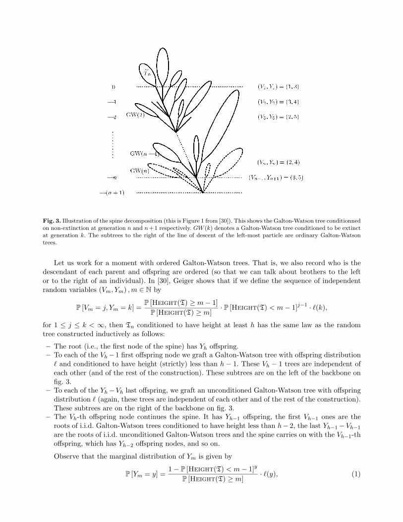
Fig. 3. Illustration of the spine decomposition (this is Figure 1 from [30]). This shows the Galton-Watson tree conditionnedon non-extinction at generation n and n+1 respectively. GW (k) denotes a Galton-Watson tree conditioned to be extinctat generation k. The subtrees to the right of the line of descent of the left-most particle are ordinary Galton-Watsontrees.

Let us work for a moment with ordered Galton-Watson trees. That is, we also record who is thedescendant of each parent and offspring are ordered (so that we can talk about brothers to the leftor to the right of an individual). In [30], Geiger shows that if we define the sequence of independentrandom variables (Vm, Ym) ,m ∈ N by

P [Vm = j, Ym = k] =P [Height(T) ≥ m− 1]

P [Height(T) ≥ m]· P [Height(T) < m− 1]j−1 · ℓ(k),

for 1 ≤ j ≤ k < ∞, then Tn conditioned to have height at least h has the same law as the randomtree constructed inductively as follows:

– The root (i.e., the first node of the spine) has Yh offspring.– To each of the Vh −1 first offspring node we graft a Galton-Watson tree with offspring distributionℓ and conditioned to have height (strictly) less than h− 1. These Vh − 1 trees are independent ofeach other (and of the rest of the construction). These subtrees are on the left of the backbone onfig. 3.

– To each of the Yh −Vh last offspring, we graft an unconditioned Galton-Watson tree with offspringdistribution ℓ (again, these trees are independent of each other and of the rest of the construction).These subtrees are on the right of the backbone on fig. 3.

– The Vh-th offspring node continues the spine. It has Yh−1 offspring, the first Vh−1 ones are theroots of i.i.d. Galton-Watson trees conditioned to have height less than h− 2, the last Yh−1 −Vh−1

are the roots of i.i.d. unconditioned Galton-Watson trees and the spine carries on with the Vh−1-thoffspring, which has Yh−2 offspring nodes, and so on.

Observe that the marginal distribution of Ym is given by

P [Ym = y] =1 − P [Height(T) < m− 1]y

P [Height(T) ≥ m]· ℓ(y), (1)

The spine can be seen as a “prolific” line of descent that survives up to generation h by producing a bi-ased number of offspring, while the other individuals of the population reproduce essentially accordingto the initial offspring distribution (we refer to [30] for an explanation of the fact that trees emanatingfrom brothers to the left of the spine are conditioned not to have descendants at generation h).

Proof (proof of theorem 2). We show that in a tree sampled according to P[h], with high probabilityonly one path from the root to height r extends to a path reaching height h. Call this event A. Sincethis property is purely topological, then it does not matter whether the tree is ordered or not. Weobtain the desired result by bounding from below the probability of A by the probability that all treesemanating from the spine under height r are of height less than h−r. The independence of this familyof trees, together with the fact (easy to check) that for every integer i in the interval {1, . . . , r − 1}

P[Height(T) < h− r

∣∣Height(T) < h− i]≥ P [Height(T) < h− r] ,

enables us to write

P [A] ≥r−1∏i=0

E[P [Height(T) < h− r]Yh−i−1

]≥ E

[P [Height(T) < h− r]

Pr−1i=0 Yh−i

]. (2)

Now, as n→ +∞, all the pn,k (for k ∈ {3, . . . , n}) converge to a finite limit p∞,k , the expected progenyµ converges to 1 (recall that µ < 1 for every n), and finally the variance σ2

n converges to q3 − q2. Thelast two convergences happen exponentially fast in n, therefore the same proof as that of Theorem 3.1in [30] (in which µ = 1 for all n) shows that whenever (mn)n≥1 tends to infinity at most polynomially,we have

limn→∞

mn · P [Height(T) ≥ mn] =2σ2. (3)

Furthermore, we have the following lemma.

Lemma 6. There exist constants C3, C4 > 0 such that for every n ≥ 3,

P

[r−1∑i=0

Yh−i > rC3

]≤ C4

r.

We postpone the proof of Lemma 6 until the end of the proof of Theorem 2. Armed with (3) andLemma 6, we can come back to (2) and write for every n

P [A] ≥ E[P [Height(T) < h− r]rC3 · 1{Pr−1

i=0 Yh−i≤C3r}]

≥(

1 − C4

σ2h

)rC3

× P

[r−1∑i=0

Yh−i ≤ rC3

]

≥ e−rh

C6

(1 − C4

r

)≥ 1 − r

hC7. (4)

Note that for the third inequality, use the fact that 1−x ≥ e−2x for every x ∈ [0, 1/2]. What (4) showsis that for every n ≥ 3, if we sample a Galton-Watson tree T according to P[h], then with probabilityat least 1 − C7

rh there will be a unique spine decomposition under height r.

Proof (of lemma 6). We use Markov’s inequality (in a Chebychev-like fashion) as follows: if C3 > 0,we have for each n ≥ 3

P

[r−1∑i=0

Yh−i > rC3

]= P

[r−1∑i=0

(Yh−i − E [Yh−i]) > C3 · r −r−1∑i=0

E [Yh−i]

]

≤

E

(r−1∑i=0

(Yh−i − E [Yh−i])

)2

(C3 · r −

r−1∑i=0

E [Yh−i]

)2 . (5)

Let us show that the numerator in the right-hand side of (5) is of order r, while the denominator isof order r2 whenever C3 > 0 is large enough. These two points rely on appropriate bounds on thefirst two moments of all Yh−i’s (observe that the numerator is in fact the sum of the variances of theYh−i’s). Indeed, recall from (1) that for every k ∈ {3, . . . , n},

P[Yh−i = qk − q2

]=

1 − P [Height(T) < h− i− 1]qk−q2

P [Height(T) ≥ h− i]· pn,k

and these are the only possible values for Yh−i. Because 1 − e−x ≤ x for all x ≥ 0, we can write forevery i ≤ r − 1 :

1 − P [Height(T) < h− i− 1]qk−q2

≤ −(qk − q2

)log P [Height(T) < h− i− 1]

≤ −(qk − q2

)log P [Height(T) < h− r − 2] .

We thus have for every such integer i

1 − P [Height(T) < h− i− 1]qk−q2

(qk − q2) · P [Height(T) ≥ h− i]≤ − log P [Height(T) < h− r − 2]

P [Height(T) ≥ h].

Moreover, because λ(·) is decreasing,

λ(n)λ(n− 2)λ(k)λ(k − 2)λ(n− k)

≤ limn→∞

1λ(n)

=: Cq.

Combining the above, we arrive at

P[Yh−i = qk − q2

]≤ − log P [Height(T) < h− r − 2]

P [Height(T) ≥ h]· Cq ·

(qk − q2

)q−k(k−2)

for every n ≥ 3 and k ∈ {2, . . . , n}. This yields

E [Yh−i] ≤ − log P [Height(T) < h− r − 2]P [Height(T) ≥ h]

· Cq ·n∑

k=3

(qk − q2

)2q−k(k−2)

E[(Yh−i)

2]≤ − log P [Height(T) < h− r − 2]

P [Height(T) ≥ h]· Cq ·

n∑k=2

(qk − q2

)3q−k(k−2)

Now, by (3) we have

limn→∞

− log P [Height(T) < h− r − 2]P [Height(T) ≥ h]

= 1,

and furthermore,

∞∑k=3

(qk − q2

)2q−k(k−2) =: m1 <∞ and

∞∑k=3

(qk − q2

)3q−k(k−2) =: m2 <∞.

As a consequence, there exists C > 0 such that for every n ≥ 3, we have

r−1∑i=0

E [Yh−i] ≤ Cm1r,

and (using the independence of all Ym’s)

E

(r−1∑i=0

Yh−i − E [Yh−i]

)2 =

r−1∑i=0

Var (Yh−i) ≤ rC ′,

for a constant C ′ > 0 depending on m1 and m2. Choosing C3 > Cm1 and coming back to (5), weobtain the existence of C4 > 0 such that for every n ≥ 3,

P

[r−1∑i=0

Yh−i ≥ rC3

]≤ C4

r.

This completes the proof of Lemma 6. ⊓⊔

Proof (proof of theorem 3). Let us use again T (from the proof of theorem 2) and its spine decom-position under the additional conditioning that all trees emanating from the spine under height rare of height smaller than h− r. We write P[h][·] as a shorthand for this conditionnal probability. Byconstruction, each brother of the i-th node of the spine (0 ≤ i ≤ r−1) has no offspring with probability

e := P[T = ∅

∣∣Height(T) ≤ h− r]

=P [T = ∅]

P [Height(T) ≤ h− r]=

ℓn(0)P [Height(T) ≤ h− r]

. (6)

Brother to the right or to the left does not matter here since the condition at the denominator isstronger than Height(T) < h− i− 1 for our range of integers i. Let us use (6) to obtain some bounds(away from 0 and 1), uniform in n and i ≤ r−1, for the probability that all of the Yh−i−1 brothers ofthe i-th node of the spine have zero offspring. Because ℓ(0) = pn,2 and using (3), the right-hand sideof (6) is equivalent as n→ ∞ to

ℓ(0)1 − 2/(σ2 · h)

≃n→∞

limn→∞

λ(n)λ(2)

=: e ∈]0, 1[. (7)

Thus, if we denote α = P[h] [no nephews at height i], then by definition

α ≥ P[Yh−i = q3 − q2

]· (e)q3−q2−1

Using (1) and (3),

α ≥1 −

(1 − 2

σ2(h− i− 1)+ o

(1h

))q3−q2

2σ2(h− i)

+ o(

1h

) · pn,2 · (e)q3−q2−1

The fraction is equal to q3 − q2 + o(1/(h)), and given the expression of pn,3 as well as (7), the lowerbound on α is equivalent to

q3 − q2

q3· eq3−q2−1

λ(1)λ(3)·

∞∏j=1

(1 − 1

qj

)= eq3−q2−1

∞∏j=4

(1 − 1

qj

)∈ ]0, 1[.

Likewise,

P[h][at least one nephew at height i] ≥ P[Yh−i = q3 − q2

] (1 − (e)q3−q2−1

)≃ (1 − eq3−q2−1)

∞∏j=4

(1 − 1

qj

)∈ ]0, 1[.

Hence, since these two probabilities belong to ]0, 1[ for all n ≥ 3 and i ≤ r−1, and belong to a smallerinterval of ]0, 1[ bounded away from 0 and 1 whenever n is large enough, this provides the existenceof κl, κu ∈]0, 1[ such that for every n ≥ 3 and i ∈ {0, . . . , r − 1},

1 − κl ≤ P[h][no nephews at height i] ≤ κu. (8)

Now, let T,T′ be two trees of height at least h and such that their spine decompositions are uniqueunder height r. For every i ∈ {0, r − 1}, let γi (resp. γ′i) be the indicator function of the event thatall brothers of the i-th node of the spine have no offspring. It follows from the properties of the spinedecomposition that for every n ≥ 3, {γi, 0 ≤ i ≤ r−1} form a family of independent random variablesand by (8), we have

P[h][γi = 1

]≤ κu and P[h]

[γi = 0

]≤ κl.

Comparing the absence or presence of nephews of the spine in T and in T′, and defining the con-stant κ = max(κl, κu) < 1, we obtain:

P[h][T = T′] ≤ κr.

⊓⊔