Abstract Fluid–structure interactions occurring between awave train and an oscillating wave surge converter (OWSC)are studied in this paper using smoothed particle hydro-dynamics (SPH). SPH is an alternative numerical methodto conventional computational fluid dynamics for studyingcomplex free surface flows. A new open multi-processing(OpenMP)-based parallel SPH code is developed and testedon a wave impacting an OWSC. An incompressible SPH(ISPH) method is implemented here to avoid spurious pres-sure oscillations, and an OpenMP approach is employed dueto its relative ease of coding. The simulation results showgood agreementwith the experimental data. Theperformanceof the new parallel SPH code is also reported for the watersurge from a canonical dam break impinging on a tall squarestructure.
Meshless methods date back almost four decades. The oldestmeshless particle method is smoothed particle hydrody-namics (SPH), which was developed in the 1970s to studycompressible inviscid problems in astrophysics by Gingold
1 Mechanical Engineering Department, University of Victoria,Victoria, Canada
2 Compute Canada, Westgrid, University of Victoria, Victoria,Canada
and Monaghan (1977) and Lucy (1977). SPH is of inter-est for hydrodynamic problems due to its Lagrangian andmeshless characteristics. The interactions betweenwaves andwave energy converters (WECs), commonly lead to a largemotion of the WEC. To model these large motions, conven-tional CFD methods require expensive and complicated gridmoving algorithms. Particle-based SPH is favored for simu-lating flows with large motion since a grid is not requiredwhen solving the Lagrangian formulation of the Navier–Stokes equations. The free surface is captured implicitly inthe SPH method without the need for solving an additionalequation, such as volume-of-fluid (VOF) or level-set (LS)approaches in conventionalCFDmethods.On the other hand,the relatively expensive SPHmethod was developed to studycompressible inviscid flows (astrophysics), therefore, modi-fications are necessary for hydrodynamic applications. SPHhas been applied to a diverse range of free surface flowsfrom wave propagation in Monaghan (1994), wave breakingin Shao and Ji (2006) to dam break problems in Lee et al.(2008) andfluid–structure interactions inHenry et al. (2014b)and Rogers et al. (2010). See Monaghan (2012) for a reviewof SPH applications in free surface flows.
The pitching flap WEC hinged close to the bottom ofthe ocean is known as an oscillating wave surge converter(OWSC) (Babarit et al. 2012). It is mentioned by Babaritet al. (2012) and Folley et al. (2007b) that OWSCs aredesigned for shallowwaters to attain higher horizontal veloc-ities and pitching motions. Several experimental, analyticaland numerical studies of OWSCs have been reported. Theexperimental studies of OWSCs are mostly performed forscaled model devices in the wave tank. Henry et al. (2014b)reported the experimental study of a 1/25th-scale OWSCmodel along with numerical simulations, using both Open-FOAM (conventional CFD) and a SPH method. The timehistories of theOWSC rotation angle between the threemeth-
ods showed good agreement. The time evolution of pressureon two sensors from the SPH simulation was compared withthe experimental data and good agreement was achieved.Henry et al. (2014a) performed two-dimensional experimentson an 1/40th-scale OWSC model and compared the resultswith numerical simulations. It was concluded that the slam-ming of the model is related to the classic wedge water entryproblem (Oger et al. 2006; Zhao et al. 1996). Clabby andTease (2015) performed a series of experiments to explorethe extreme events related to a 1/20th-scale OWSC model.It was reported that the extreme pressure occurs during thebreaking waves or re-entry slamming of the flap.
It is worth pointing out that the experimental studiesare extremely important to study OWSC devices due tothe complex phenomena involved and to validate numeri-cal simulations. However, it is costly to perform parametricstudies, such as changing flap size, wave conditions andtank dimensions in the experimental campaigns. Therefore,numerical simulations are also extremely important to effi-ciently design the experiments. Potential flow methods havebeen extensively applied to ocean engineering problems.Although these methods are restricted to solving linear invis-cid equations, they provide valuable insight for the problemin a reasonable time. Studies based on potential methodsapplied to OWSCs can be found in Folley et al. (2007a) andRenzi and Dias (2012, 2013). OWSCs are designed for shal-low waters, hence they may experience extreme wave loadsas mentioned by Wei et al. (2015) and Henry et al. (2014b).Also, the interactions betweenwaves andOWSCmay includecomplex phenomena such as slamming, wave over-topping,air entrainment and turbulence (Wei et al. 2015). There-fore, potential flowmethods have limitations in capturing thedetails, especially the nonlinearities, involved in the interac-tions of OWSCs and shallow waters.
Computational fluid dynamics (CFD) simulation using thefull Navier–Stokes equations is an alternative approach topotential methods. It provides a more accurate descriptionof the whole flow including the interactions between wavesand OWSC. However, Navier–Stokes solvers are computa-tionally more expensive than potential flow methods. Weiet al. (2015) performed numerical simulations using ANSYSFLUENT to investigate the viscous and scaling effects onOWSCs. The time histories of different pressure sensors,rotation angle and vortex shedding from the wave impact fortwo wave conditions were compared with the experimentaldata. It was concluded that the viscous effects are negligiblefor wide flaps. Schmitt and Elsaesser (2015) proposed a newmoving mesh approach for OWSCs using OpenFOAM andcompared simulation resultswith experiments for regular andirregular waves.
Rafiee and Dias (2013) performed 2D and 3D simulationsof wave interactions with OWSC using SPH. The k − ε tur-bulence model was used along with the SPHmethod to study
the effects of wave loads on the OWSCs. It was concludedthat 3D simulations provide more accurate estimation of thepressure peaks and angles of rotation compared to the 2Dsimulations.
In this paper, we report our work on wave interaction withan OWSC device. A custom SPH method was implementedusing parallel computing and an incompressible formulationof the governing equations. The methodology we followedand the parallel scheme used to implement a new OpenMPSPH are discussed in Sects. 2.1 and 3, respectively. A classi-cal wedge water entry problem is presented in Sect. 4.2 as aslamming benchmark test case. The experimental setup sim-ulated is described in Sect. 4.3.1. The numerical results ofthe simulations are compared with the available experimen-tal data in Sect. 4.3.2. The performance of the new parallelSPH code is also reported for a dam break on a tall squarestructure (Sect. 4.1).
2 Methodology
2.1 Governing equations
In the SPH method, the Navier–Stokes equations are solvedin a Lagrangian formulation, thus they read:
DuDt
= − 1
ρ∇ p + g + ν∇2u, (1)
where ρ is the fluid particle density, u is the particle velocityvector, t is time, p is the particle pressure, g is the gravi-tational acceleration vector and ν is the kinematic viscosity(it should be mentioned that the bold parameters representvector quantities in this paper). In SPH, a general function isapproximated as (Monaghan 1992):
A(r) ≈∫
A(x)W (r − x, h)dx, (2)
where A(r) is the function of interest at position r, W (r −x, h) is the smoothing or kernel function, r is the positionvector, h is the smoothing length by which neighboring par-ticles are defined. The particle approximation of the aboveintegral is written by replacing the integral with a summationas
Ai ≈N∑j=1
A jW (r − rj, h)Vj , (3)
where N is the number of neighboring particles and Vj is thevolume of particle j (particle j is a neighbor to i). In thispaper, the fifth-order Wendland kernel proposed by Wend-land (1995) is used:
123
J. Ocean Eng. Mar. Energy (2016) 2:301–312 303
W (q) = Wc
{(1 + 2q)
(1 − q
2
)40 ≤ q ≤ 2
0 q ≥ 2,(4)
where Wc = 21/16πh3 in 3D and q = |ri − rj|/h. Thesmoothing length is set to h = 1.5�r for 3D cases, where�r is the initial particle spacing. The gradient operator isused from Monaghan (1992) as
(1
ρ∇A
)i=
∑j
m j
(Ai
ρ2i
+ A j
ρ2j
)∇iWi j . (5)
In this paper, the Laplacian operator is adopted from Shaoand Lo (2003) as
∇ ·(∇A
ρ
)i= ∑
j
8m j
(ρi + ρ j )2
Ai jri j · ∇iWi j
r2i j + η2, (6)
where Ai j = Ai − A j , η = 0.1h and ri j = ri − r j . InSPH, there are two main approaches to calculate pressure:weakly compressible SPH (WCSPH) and incompressibleSPH (ISPH). WCSPH is the original SPH method appliedto simulate free surface flows. In this approach, the fluidis considered to be weakly compressible and the equationof state is used to calculate pressure. A promising alterna-tive to WCSPH is incompressible SPH (ISPH) proposed byCummins and Rudman (1999). This approach is based on atwo-step projection method widely used in Eulerian-basedCFDmethods (Chorin 1968). In this approach, in the predic-tion step, the intermediate velocity (u∗) is calculated usingthe viscous and body forces, without pressure forces as
u∗i = ui (t) + Δt (g + ν∇2ui ). (7)
Subsequently, the intermediate position is calculated by:
r∗i = ri (t) + Δtu∗
i . (8)
In the ISPHmethod, Poisson’s equation is solved for pressureat each time step as
∇ ·(∇ p
ρ
)i= ∇ · u∗
i
Δt. (9)
The left hand side of Poisson’s equation is discretized usingEq. 6 as
∇ ·(∇ p
ρ
)i=
∑j
8m j
(ρi + ρ j )2
pi jri j · ∇iWi j
r2i j + η2, (10)
and for the right hand side, the term proposed by Khayyeret al. (2009) is implemented as
∇ · u∗i = ∑
jV j (u∗
j − u∗i )∇iWi j . (11)
Hence, Poisson’s equation is written as
∑j
8m j
(ρi + ρ j )2
pi jri j · ∇iWi j
r2i j + η2= −1
�t
∑jV j (u∗
i − u∗j )∇iWi j .
(12)
Poisson’s equation is then solved explicitly using the sameprocedure proposed by Hosseini et al. (2007). Hence, thepressure for a fluid particle, pi , is obtained by:
pi =∑
j Ai j p j + RHSi∑j Ai j
, (13)
where
RHSi = −1�t
∑j
m j
ρ j(u∗
i − u∗j )∇iWi j , (14)
Ai j = ∑j
8m j
(ρi + ρ j )2
ri j · ∇iWi j
r2i j + η2. (15)
In the correction step, incompressibility is achieved by cor-recting the velocity using the pressure force as
ui (t + Δt) = u∗i + Δt
(− 1
ρ∇ pi
). (16)
The positions are updated at the end of each time step as
ri (t + Δt) = ri (t) + Δt
(ui (t + Δt) + ui (t)
2
). (17)
SPH is a general 3D fluid simulation method, but the scaleOWSCmodel is constrained only to pitchmotion (one degreeof freedom (DOF)). To calculate the motions and forces inthe fluid–structure interaction, the rigid body equations aresolved for one structural DOF (pitch motion) along with the3D Navier–Stokes equations in particle form as
dUdt
=∑
i fiMbody
+ g, (18)
dω
dt=
∑i τ i
Ibody, (19)
τi = (ri − R) × fi , (20)
where Mbody is the mass of the rigid-body, Ibody is themoment of inertia about the fixed rotation axis,R is the posi-tion of center of mass for the rigid-body,U is the transitionalvelocity, ω is the rotational velocity,
∑i τ i is the sum of the
moments on the rigid-body particles and∑
i fi is the sumof the forces on the rigid-body particles which is calculatedbased on the surrounding fluid particles. Subsequently, thevelocity of the rigid-body particles are obtained as
ui = U + ω × (ri − R). (21)
123
304 J. Ocean Eng. Mar. Energy (2016) 2:301–312
The positions of the rigid-body particles are updated by usingEq. 17.
2.2 Boundary conditions
Applying solid boundary conditions is the most challengingtask in the SPH method. The three main methods reportedto simulate solid boundaries in SPH are: repulsive bound-ary particles (Monaghan 1994; Monaghan and Kos 1999),dummy boundary particles (Koshizuka et al. 1998; Lo andShao 2002) and ghost boundary particles (Colagrossi andLandrini 2003). In the repulsive boundary particles approach,a single line of boundary particles are placed on the edge ofthe solid boundary, exerting a repulsive force on the fluidparticles approaching them. In the dummy boundary parti-cles approach, several layers of particles are placed on theedge and inside the solid boundary. In the ghost boundaryparticles approach, the position of ghost particles is deter-mined by reflection of the fluid particles position through thesolid boundary. The pressure of the ghost particles are thesame as their corresponding fluid particles (in the presenceof the gravity, there will be an additional hydrostatic pres-sure). Each of these methods has advantages and drawbacksin terms of accuracy and computational complexity.
In this paper, fixed dummy particles are used both forsolid boundary particles on tank walls and on the OWSCflap. The dummy particles have the advantage of being easyto implement, especially in a parallel SPH method. In thecurrent work, we used the method described by Adami et al.(2012) to calculate the pressure for the boundary particlesfrom the surrounding fluid particles as
ps =∑
i piWsi + (g − as)∑
i ρirsiWsi∑i Wsi
, (22)
where ps is the pressure for a solid boundary particle, i is theindex for the surrounding fluid particle and as is accelerationof the wall.
The free surface particles are identified to apply theDirich-let boundary condition (p = 0) in Poisson’s equation. In theISPH method the density for each particle is constant. How-ever, to determine free surface particles a fake density (ρ f )is calculate for each fluid particle as
ρ f (i) =∑j
m jWi j . (23)
ρ f is not involved in solving the governing equations and isonly used to determine the free surface particles. The criteriaused for defining a free surface particle is
ρ f ≤ 0.9ρ0, (24)
where ρ0 = 1000 kg/m3. The particles that meet the abovecriteria are considered to be free surface particles.
3 Parallelization scheme
The SPH method is typically computationally more expen-sive than Eulerian-based CFD methods. Therefore, paral-lelization methods are required to improve the performanceof the method, especially for 3D simulations. CPU-basedand GPU-based parallelizations are the two main tech-niques that can be employed for SPH parallelization (Her-manns 2002). The CPU-based parallelization is divided intoshared-memory and distributed memory parallelizations.The shared-memory approach assumes that the processingunits share a common memory (as is the case for multi-coreprocessors) that the parallel tasks canuse to communicate andshare variables with each other. The thread model is usuallyused when implementing a shared memory parallelization.More specifically, OpenMP, a standard for implementingthe thread model by adding directives to the code, is arelatively easy way to parallelize an existing serial code.The distributed memory method uses the common memoryassumption and requires the parallel tasks to communicateby exchanging messages. MPI (Message Passing Interface)is a standard for distributed memory parallelization. GPU-based parallelization relies on GPUs to schedule and executethe parallel tasks. CUDA, openCL and openACC are thecommon programming standards for GPU-based implemen-tations. Several approaches have been applied to parallelizethe SPH method using these standards. Ferrari et al. (2009)proposed a parallelization schemes using the MPI standardto study free surface flows.Marrone et al. (2012) studied shipwave breaking patterns using 3D hybrid MPI and OpenMPstandards. A review of CPU-based parallelization implemen-tations for the SPH method in free surface flows is availableby Gomez-Gesteira et al. (2012). GPUs have been applied toSPH methods recently. A review of GPU-based paralleliza-tion implementations for the SPH method is available byCrespo et al. (2015).
The SPH method is both Lagrangian and meshless.Although these two features are attractive in modellingcomplex free surface flows, they cause difficulties in par-allelization schemes (Marrone et al. 2012). Unlike the fixedgrids in CFD mesh-based methods, particles move due tothe Lagrangian nature of the method and the neighboringparticles do not remain the same throughout the simulation.Hence, as mentioned by Marrone et al. (2012), the parallelscheme applied to the SPH method must take into accountthis specific characteristic.
To save computational costs in SPH, only the contribu-tion of neighboring particles (ri j ≤ kh) are calculated inthe simulation. The link list searching algorithm reported in
123
J. Ocean Eng. Mar. Energy (2016) 2:301–312 305
NW N NE
E NNW NE
E
SESSW
W
kh
kh
i
j
i
j
jj
j j
j
j j j
j
j
Inner cells Outter cells Sample water particles
Fig. 1 Two-dimensional underlying grid for the link list algorithm.Cells enclosed by red contours are handled by the same thread (colorfigure online)
Gomez-Gesteira et al. (2012) is adopted here to search forthe neighboring particles. In this algorithm, the computa-tional domain is divided into square cells of side kh (kernelradius). The particle in each cell only interacts with particlesin neighboring cells; eight cells in 2D are shown in Fig. 1.The sweep of the link list search starts from the lower leftend and in each sweep, only the E, N , NW, NE cells areinvolved to prevent repeating particle interactions (4 cellsout of 8 neighboring cells Gomez-Gesteira et al. 2012). Thesame procedure will be applied in 3D; interactions of 13 cellsout of 26 neighboring cells will be calculated. In the currentwork, we take the advantage of this approach to parallelizethe code using an OpenMP standard.
Due to the Lagrangian nature of the method special treat-ments are required at the particles along the processor domainboundaries. These particlesmay require information from theneighboring particles located on another processor domain.This is handledby introducingghost cells byGomez-Gesteiraet al. (2012) or buffer particles by Marrone et al. (2012). Inthis paper, the domain decomposition is performed spatiallyin 3D as shown in Fig. 1 for a 2D case (for simplicity) butthe same applies for the 3D case. Here, we divide the cells ineach thread to be the inner cells and the outer cells. The lastcell in each thread is assigned to be the outer cell. The outercells are available for both threads. The domain decomposi-tion is performed in this way in order to avoid two or moreparallel threads having access to the same data. Since eachthread will update its particles, we need to make sure that theother thread has access to the old values instead of the newones.
For the inner cells, the same procedure that was performedfor a single core is performed. The sweep starts from thelower left end and in each sweep, only the E, N , NW, NEcells are involved as shown in Fig. 1.
For the outer cells, the interaction between particles isconsidered in all eight neighboring cells in 2D and 26 cellsin 3D. The first sweep is performed on E, N , NW, NE cells(yellow sweep in Fig. 1). If the cells are within the samethread then both particles i and j will be updated. If one of
the cells is from the adjacent thread only particle i will beupdated. The second sweep is performed on W, S, SW, SEcells (pink sweep in Fig. 1). If cells belong to the same thread,none of the particles i or j are updated, but if they belong tothe adjacent thread only particle i will be updated. By usingthis approach, the same procedure of finding neighboringparticles is applied for parallelization without introducingany ghost cells or buffer particles.
4 Test cases
4.1 Test case 1: dam break on a structure
Dam-break problems are typically used as benchmark testcases for SPH codes. In this paper, the dam-break on a tallstructure is first simulated to test the performance of thenew OpenMP SPH code. The dam-break benchmark studiesare important to investigate the influence of severe floodingevents such as tsunamis on shoreline structures. The experi-mental set up of Yeh and Petroff reported byGómez-GesteiraandDalrymple (2004) is used tovalidate theparallelOpenMPSPH code. Dimensions of the experiment and the tall squarestructure are shown in Fig. 2. A layer of approximately 1 cmof water existed on the bottom of the tank, before the dambreaks, at t = 0 s. In the experiment, asmentioned inGómez-Gesteira andDalrymple (2004), the velocity in the x-direction
61
25
12
24
125040 58
30
75
Obstacle
Gate
Water
z
x
y
x
Fig. 2 Schematic of the validation case: dam break in the vicinity ofa tall structure (dimensions in cm). Experiment reported by Gómez-Gesteira and Dalrymple (2004)
123
306 J. Ocean Eng. Mar. Energy (2016) 2:301–312
0 0.5 1 1.5−0.5
0
0.5
1
1.5
2
2.5
t(s)
u (m
/s)
Experiment in Gomez−Gesteira and Dalrymple (2004)SPH, particle size=2 cmSPH, particle size=1.5 cmSPH, particle size=1.0 cmSPH, particle size=0.8 cm
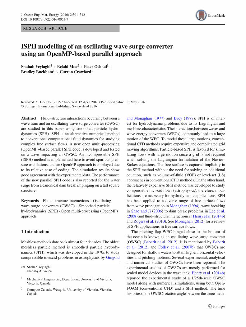
Fig. 3 Magnitude of the fluid velocity in x-direction (u) at x = 0.754m, y = 0.31 m, z = 0.026 m as a function of time for dam breakexperiment
was measured at 2.6 cm from the bottom of the tank and14.6 cm upstream of structure center.
For this simulation, the particle size was set to �x =0.01 m, �y = 0.01 m, �z = 0.01 m which resulted in298,463 total particles. The simulations were performed ona localmachine using 16 processors [model Intel(R)Xeon(R)CPU E5-2630 0 @ 2.30 GHz].
The time history of water velocity in the x-direction at themeasured point is compared with experimental data in Fig. 3.To calculate the velocity, the same kernel function for simu-lation is used to interpolate neighboring particles’ velocity atthe specified point. It is shown in Fig. 3 that the SPH resultsare in good agreement with the experimental data. A con-vergence study is performed for four particle sizes and theresults are presented in Fig. 3. It is shown that by increasingthe particle resolution the maximum velocity value is cap-tured more accurately.
The particle representation of the domain (water particlesand the structure) at t = 0.9 s is shown in Fig. 4. Particles arecoloredwith their velocitymagnitude. At t = 0.9 s, water hasimpacted the structure and is getting closer to the end of thewave tank. The non-uniform distribution of the particles nearthe front of the dam could be due to the kernel truncation inthe ISPHmethod which was mentioned by Lind et al. (2012)and Xu et al. (2009).
The wall clock time (execution time) for 500 time stepsof the simulation with 298,463 particles for 1, 2, 4 and 16threads is shown in Fig. 5. The wall clock time is comparedfor different combinations of threads in this figure (the x andy-directions are chosen since the initial water depth is 0.3 min z-direction). It is shown that by increasing the numberof threads from 1 to 16 the execution time decreases. Thespeedup for a parallel code is defined by Quinn (2003) as
Fig. 4 Flow due to the dam break on the tall structure at t = 0.9 s
1*1 2*1 1*2 4*1 2*2 1*4 16*1 4*4 1*160
500
1000
1500
2000
2500
3000
Thread combinations in X−direection × Y−direction
Wal
l Clo
ck T
ime
(s)
Fig. 5 Wall clock time for 500 time steps for different thread combi-nations for 1, 2, 4 and 16 threads
S = Tserial/Tparallel, where the Tserial is the serial executiontime and Tparallel is the parallel execution time. As expected,the speedup does not scale particularly well for the OpenMPapproach. Possible explanations for this include: the timespent on the serial part of the code, joining and forking andthe time wasted by the threads waiting for other threads toperform their jobs due to load imbalance. As shown in Fig. 6,by increasing the number of particles, decomposing threadsin the y-direction decreases the execution time more thandecomposing them in the x-direction. The reason is that at500 time steps (t = 0.25 s), water particles accelerate towardthe tall structure but they have not yet reached the structure.Therefore, there are more particles in the y-direction anddecomposing more threads in that direction reduces the wallclock time (Fig. 6).
)Threads in x−direction=1,Threads in y−direction=1Threads in x−direction=1,Threads in y−direction=2
Fig. 6 Wall clock time for 500 time steps for different number of par-ticles
4.2 Test case 2: wedge water entry simulation
The 2D wedge water entry problem is chosen for simulationto test the accuracy of the ISPH method before modeling thewave impacting an OSWC. The experiment of Zhao et al.(1996) is simulated in this paper where a symmetric wedgeis dropped on a free surface of a water tank at rest. Theschematic of the wedge and locations of pressure sensors areshown in Fig. 7. At t = 0 s, the wedge with total mass of241 kg is dropped with the initial vertical velocity of −6.15m/s. The total number of particles used for ISPH simulationis 85,983 in 2D. In Figs. 8 and 9 fluid particles are shownwith by their pressure at t = 0.00435 s and t = 0.0158 s,respectively. The formation of two jets along the boundariesof the wedge and the free surface deformation are clear inboth figures.
In Figs. 10 and 11 the pressure along the boundary ofthe wedge are shown at t = 0.00435 s and t = 0.0158s, respectively. In these figures, as mentioned by Liu et al.(2014), the p0 = 0, V is the vertical velocity of the wedge,Z is the vertical coordinate of the wedge boundary particles,Z0 is the initial vertical coordinate of the keel and |Zkeel| is
50
P1P2
P3P4
P5
2.5
7.5 12.5
17.5
2.530o
Fig. 7 Schematic of the wedge (dimensions in cm)
Fig. 8 Particles are shown with their pressure at t = 0.00435 s
Fig. 9 Particles are shown with their pressure at t = 0.0158 s
−1 −0.5 0 0.5 10
2
4
6
8
10
2(p−
p 0)/(ρ
V2 )
(Z−Z0)/|Z
keel|
Exp, Zhao et al.(1997)WCSPH, Oger et al. (2006)Current study
p1
p2
Fig. 10 Pressure along the boundary of the wedge at t = 0.00435 s
the total displacement of the keel. In Figs. 10 and 11, resultsof the current simulation are compared with the experimentaldata of Zhao et al. (1996) and theWCSPH study of Oger et al.(2006). At t = 0.00435 s both SPH studies underestimate thepressure. The reason was mentioned by Oger et al. (2006) tobe a compressible effect caused by abrupt change of flowat the beginning of the simulation. At t = 0.0158 s bothmethods slightly overestimate the experimental data up tosensor P5. This is due to the 3D effects mentioned by Zhaoet al. (1996) and Oger et al. (2006).
123
308 J. Ocean Eng. Mar. Energy (2016) 2:301–312
−1 −0.5 0 0.5 10
2
4
6
8
102(
p−p 0)/(
ρ V
2 )
(Z−Z0)/|Z
keel|
Exp, Zhao et al.(1997)WCSPH, Oger et al. (2006)Current study
P5
P4P3P2
P1
Fig. 11 Pressure along the boundary of the wedge at t = 0.0158 s
300
400340
20060
40150
260
Axis of rotation
MWL
P6(P1)
P5(P2)
P4(P3)
Fig. 12 Schematic of the flap (dimensions in mm)
4.3 Test case 3: wave impacting an oscillating wavesurge converter
4.3.1 Experiment
The1:20 scalemodel ofResoluteMarineEnergysSurgeWECis chosen for simulation in this paper. As described in ClabbyandTease (2015), this device is smaller than theAquamarinesOyster, therefore the device response to the wave impactbehavior might be different than the already studied Oyster.
The experimentswere conducted atOrionEnergyCentre’swave tank. The wave tank is 18.2 m long and 6 m wide(Fig. 13). The waves are generated using eight wavemakersacross the width on the left end of the tank (Fig. 13). TheOWSC model is located at 10.8 m from the wavemakers.The waves are absorbed at the end of the tank by a slopedbeach (Fig. 13).
The 1:20 scalemodel is a flap of 0.4mwidth, 0.3m height,and 0.06 m thickness and was hinged 0.05 m above the tankbottom (Fig. 13). The model is made of 6.3 mm thick steelplate with an aluminum skeleton and foam body [for more
Pad
dles
Flap
Beach0.91 2.44 1.22
18.2
d=0.7 10.8
1401
10
Fig. 13 Schematic of the wave tank (dimensions in m)
details about the model see Clabby and Tease (2015)]. SixKeller series 10 pressure sensors were placed on the frontand rear faces of the flap. Sensors 4–6 were placed on thefront face of the flap and sensors 1–3 placed on the rear faceof the flap. The position of the pressure sensors are shown inFig. 12.
A series of experiments were performed to study theextreme loads on the SurgeWEC 1:20 scale model by Clabbyand Tease (2015). Three water depths were tested underfour extreme sea conditions, ten monochromatic wave andthree irregular waves. In this paper, experimental results fora monochromatic wave were chosen to validate the SPHresults.
4.3.2 SPH simulations
The 1:20 scale model of the SurgeWEC that was describedin Sect. 4.3.1 is simulated herein using the ISPH approach.The numerical flap has the same dimensions of the experi-mental flap: 0.4 mwidth, 0.3 m height, and 0.06 m thickness.The SPH simulation is performed in a 18.2 m (length)× 4 m(width) × 1.2 m (height) numerical tank where the flap ispositioned at 10.8 m from the wavemaker. To save compu-tational cost, we choose the numerical wave tank’s width tobe 2.0 m smaller than the experimental width. The numericalwavemaker is forced to have sinusoidal motion based on thetheory given by Dalrymple and Dean (1991):
x = S
2sin
(2π
T
), (25)
where x is the motion of the wavemaker in the x-direction, Tis the wave period and S is the stroke of the wavemaker. Thewave profile used for the simulation has a height of Hw =0.15 m and a period of T = 1.34 s.
The still water depth is 0.7 m and the numerical wave-makerwas calibrated to produce awave of height 0.15m.Theparticle dimensions are set to �x = �y = �z = 0.02 m,which leads to 4,222,746 total particles. To avoidwave reflec-tion, the damping region similar to the relaxation zoneproposed by Lind et al. (2012) is applied to the zone close tothe far downstream wall.
123
J. Ocean Eng. Mar. Energy (2016) 2:301–312 309
(a) t = 10.6 s
(b) t = 10.6 s
(c) t = 11.1 s
(d) t = 11.6 s
Fig. 14 Particles in the domain are colored by their pressure at threetime steps a shown in 3D, b–d shown in 2D
(b) t = 12.1 s where θ ≈ 30◦.
(a) t = 11.6 s where θ ≈ −36◦.
Fig. 15 Pressure field on the flap face
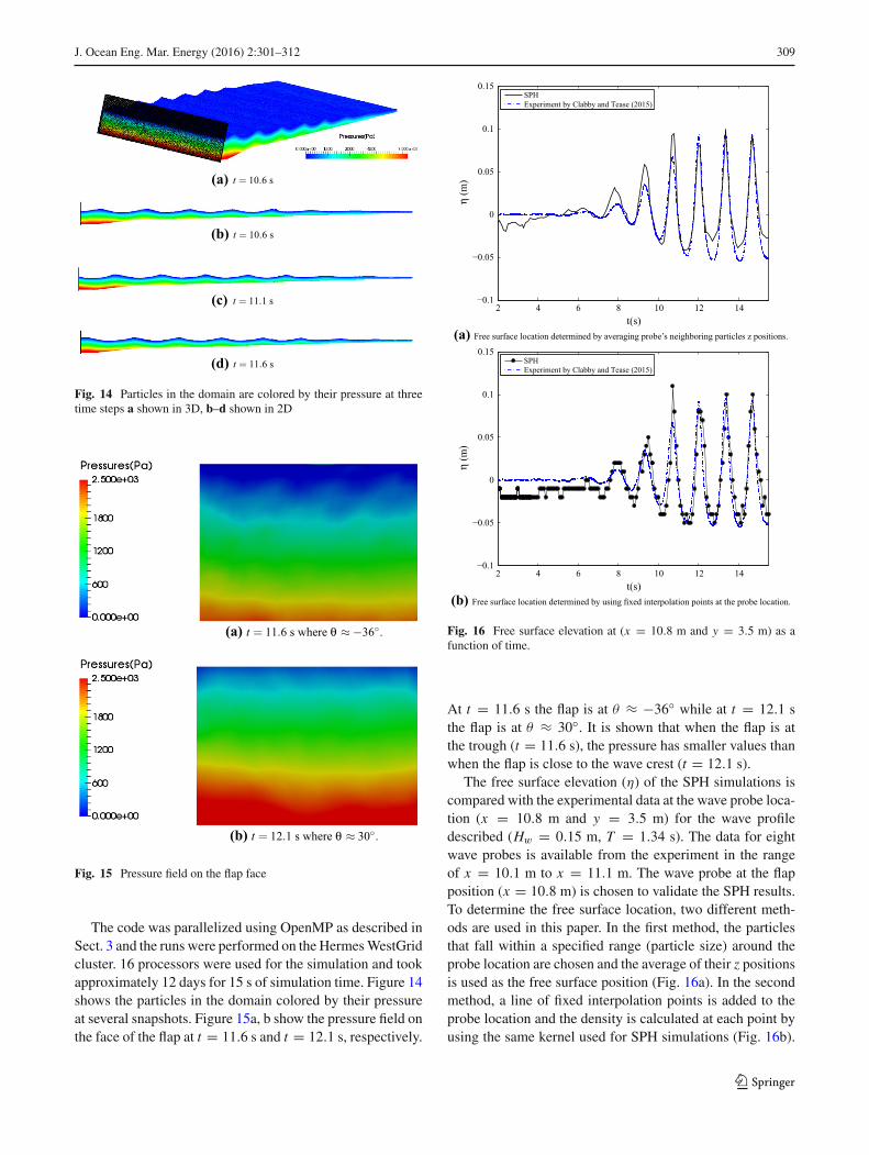
The code was parallelized using OpenMP as described inSect. 3 and the runs were performed on the HermesWestGridcluster. 16 processors were used for the simulation and tookapproximately 12 days for 15 s of simulation time. Figure 14shows the particles in the domain colored by their pressureat several snapshots. Figure 15a, b show the pressure field onthe face of the flap at t = 11.6 s and t = 12.1 s, respectively.
2 4 6 8 10 12 14−0.1
−0.05
0
0.05
0.1
0.15
η (m
)
t(s)
SPHExperiment by Clabby and Tease (2015)
(a) Free surface location determined by averaging probe’s neighboring particles z positions.
2 4 6 8 10 12 14−0.1
−0.05
0
0.05
0.1
0.15
η (m
)
t(s)
SPHExperiment by Clabby and Tease (2015)
(b) Free surface location determined by using fixed interpolation points at the probe location.
Fig. 16 Free surface elevation at (x = 10.8 m and y = 3.5 m) as afunction of time.
At t = 11.6 s the flap is at θ ≈ −36◦ while at t = 12.1 sthe flap is at θ ≈ 30◦. It is shown that when the flap is atthe trough (t = 11.6 s), the pressure has smaller values thanwhen the flap is close to the wave crest (t = 12.1 s).
The free surface elevation (η) of the SPH simulations iscompared with the experimental data at the wave probe loca-tion (x = 10.8 m and y = 3.5 m) for the wave profiledescribed (Hw = 0.15 m, T = 1.34 s). The data for eightwave probes is available from the experiment in the rangeof x = 10.1 m to x = 11.1 m. The wave probe at the flapposition (x = 10.8 m) is chosen to validate the SPH results.To determine the free surface location, two different meth-ods are used in this paper. In the first method, the particlesthat fall within a specified range (particle size) around theprobe location are chosen and the average of their z positionsis used as the free surface position (Fig. 16a). In the secondmethod, a line of fixed interpolation points is added to theprobe location and the density is calculated at each point byusing the same kernel used for SPH simulations (Fig. 16b).
123
310 J. Ocean Eng. Mar. Energy (2016) 2:301–312
2 4 6 8 10 12 14−50
−40
−30
−20
−10
0
10
20
30
40
50θ(
°)
t(s)
SPHExperiment by Clabby and Tease (2015)
Fig. 17 Angular position of the flap as a function of time
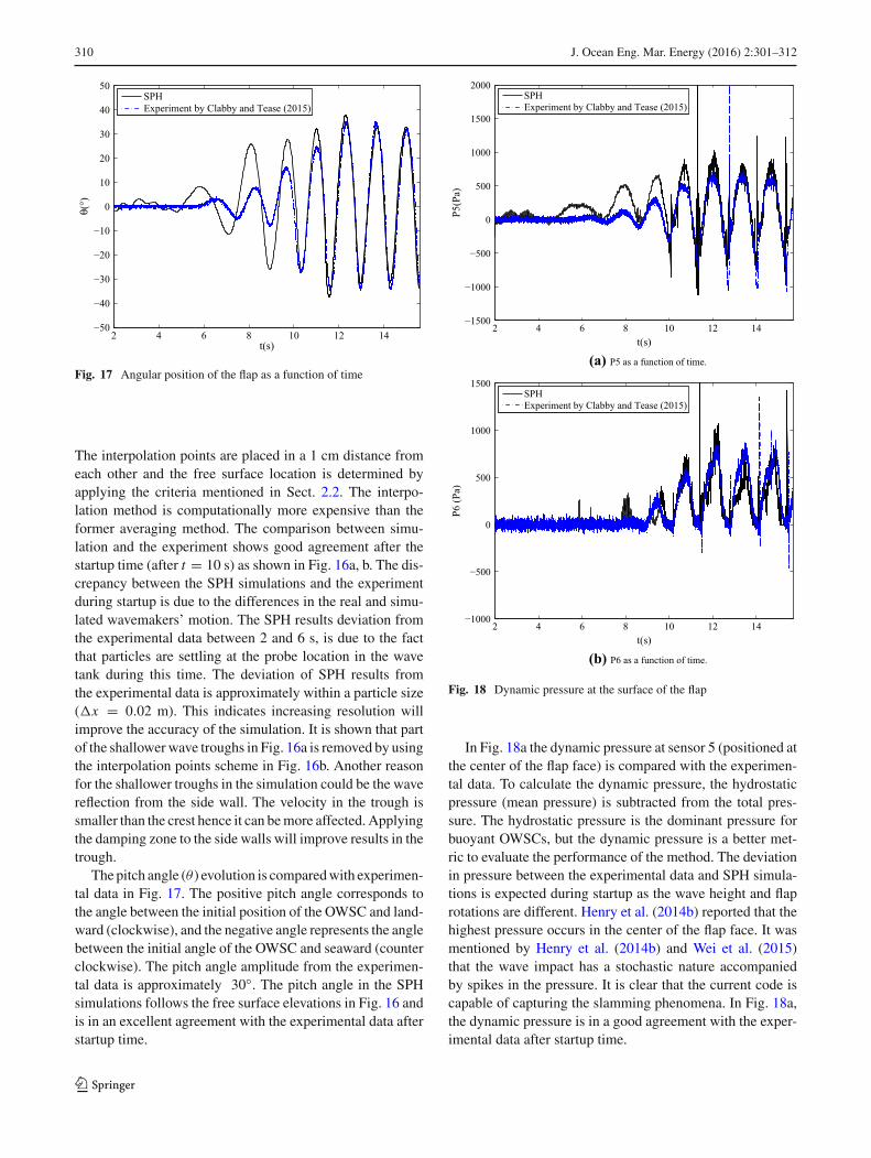
The interpolation points are placed in a 1 cm distance fromeach other and the free surface location is determined byapplying the criteria mentioned in Sect. 2.2. The interpo-lation method is computationally more expensive than theformer averaging method. The comparison between simu-lation and the experiment shows good agreement after thestartup time (after t = 10 s) as shown in Fig. 16a, b. The dis-crepancy between the SPH simulations and the experimentduring startup is due to the differences in the real and simu-lated wavemakers’ motion. The SPH results deviation fromthe experimental data between 2 and 6 s, is due to the factthat particles are settling at the probe location in the wavetank during this time. The deviation of SPH results fromthe experimental data is approximately within a particle size(�x = 0.02 m). This indicates increasing resolution willimprove the accuracy of the simulation. It is shown that partof the shallowerwave troughs in Fig. 16a is removed by usingthe interpolation points scheme in Fig. 16b. Another reasonfor the shallower troughs in the simulation could be the wavereflection from the side wall. The velocity in the trough issmaller than the crest hence it can bemore affected. Applyingthe damping zone to the side walls will improve results in thetrough.
The pitch angle (θ ) evolution is comparedwith experimen-tal data in Fig. 17. The positive pitch angle corresponds tothe angle between the initial position of the OWSC and land-ward (clockwise), and the negative angle represents the anglebetween the initial angle of the OWSC and seaward (counterclockwise). The pitch angle amplitude from the experimen-tal data is approximately 30◦. The pitch angle in the SPHsimulations follows the free surface elevations in Fig. 16 andis in an excellent agreement with the experimental data afterstartup time.
2 4 6 8 10 12 14−1500
−1000
−500
0
500
1000
1500
2000
P5(P
a)
t(s)
SPHExperiment by Clabby and Tease (2015)
(a) P5 as a function of time.
2 4 6 8 10 12 14−1000
−500
0
500
1000
1500
P6 (P
a)
t(s)
SPHExperiment by Clabby and Tease (2015)
(b) P6 as a function of time.
Fig. 18 Dynamic pressure at the surface of the flap
In Fig. 18a the dynamic pressure at sensor 5 (positioned atthe center of the flap face) is compared with the experimen-tal data. To calculate the dynamic pressure, the hydrostaticpressure (mean pressure) is subtracted from the total pres-sure. The hydrostatic pressure is the dominant pressure forbuoyant OWSCs, but the dynamic pressure is a better met-ric to evaluate the performance of the method. The deviationin pressure between the experimental data and SPH simula-tions is expected during startup as the wave height and flaprotations are different. Henry et al. (2014b) reported that thehighest pressure occurs in the center of the flap face. It wasmentioned by Henry et al. (2014b) and Wei et al. (2015)that the wave impact has a stochastic nature accompaniedby spikes in the pressure. It is clear that the current code iscapable of capturing the slamming phenomena. In Fig. 18a,the dynamic pressure is in a good agreement with the exper-imental data after startup time.
123
J. Ocean Eng. Mar. Energy (2016) 2:301–312 311
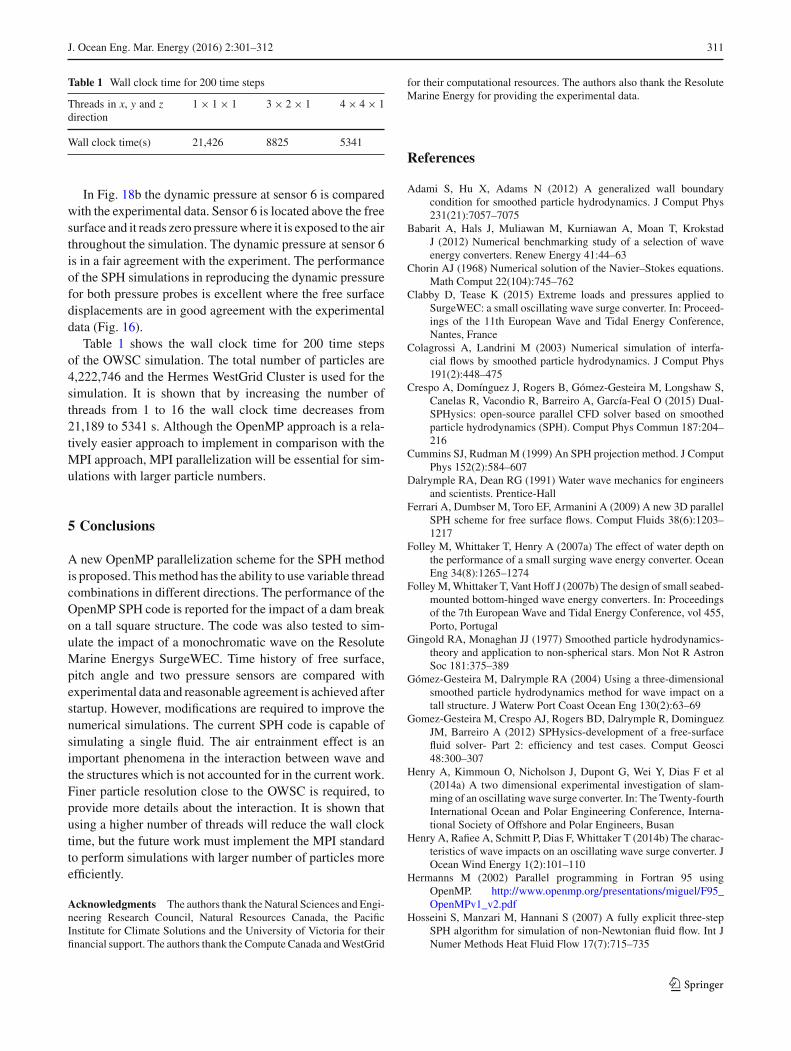
Table 1 Wall clock time for 200 time steps
Threads in x, y and zdirection
1 × 1 × 1 3 × 2 × 1 4 × 4 × 1
Wall clock time(s) 21,426 8825 5341
In Fig. 18b the dynamic pressure at sensor 6 is comparedwith the experimental data. Sensor 6 is located above the freesurface and it reads zero pressurewhere it is exposed to the airthroughout the simulation. The dynamic pressure at sensor 6is in a fair agreement with the experiment. The performanceof the SPH simulations in reproducing the dynamic pressurefor both pressure probes is excellent where the free surfacedisplacements are in good agreement with the experimentaldata (Fig. 16).
Table 1 shows the wall clock time for 200 time stepsof the OWSC simulation. The total number of particles are4,222,746 and the Hermes WestGrid Cluster is used for thesimulation. It is shown that by increasing the number ofthreads from 1 to 16 the wall clock time decreases from21,189 to 5341 s. Although the OpenMP approach is a rela-tively easier approach to implement in comparison with theMPI approach, MPI parallelization will be essential for sim-ulations with larger particle numbers.
5 Conclusions
A new OpenMP parallelization scheme for the SPH methodis proposed. Thismethod has the ability to use variable threadcombinations in different directions. The performance of theOpenMP SPH code is reported for the impact of a dam breakon a tall square structure. The code was also tested to sim-ulate the impact of a monochromatic wave on the ResoluteMarine Energys SurgeWEC. Time history of free surface,pitch angle and two pressure sensors are compared withexperimental data and reasonable agreement is achieved afterstartup. However, modifications are required to improve thenumerical simulations. The current SPH code is capable ofsimulating a single fluid. The air entrainment effect is animportant phenomena in the interaction between wave andthe structures which is not accounted for in the current work.Finer particle resolution close to the OWSC is required, toprovide more details about the interaction. It is shown thatusing a higher number of threads will reduce the wall clocktime, but the future work must implement the MPI standardto perform simulations with larger number of particles moreefficiently.
Acknowledgments The authors thank theNatural Sciences and Engi-neering Research Council, Natural Resources Canada, the PacificInstitute for Climate Solutions and the University of Victoria for theirfinancial support. The authors thank the Compute Canada andWestGrid
for their computational resources. The authors also thank the ResoluteMarine Energy for providing the experimental data.
References
Adami S, Hu X, Adams N (2012) A generalized wall boundarycondition for smoothed particle hydrodynamics. J Comput Phys231(21):7057–7075
Babarit A, Hals J, Muliawan M, Kurniawan A, Moan T, KrokstadJ (2012) Numerical benchmarking study of a selection of waveenergy converters. Renew Energy 41:44–63
Chorin AJ (1968) Numerical solution of the Navier–Stokes equations.Math Comput 22(104):745–762
Clabby D, Tease K (2015) Extreme loads and pressures applied toSurgeWEC: a small oscillating wave surge converter. In: Proceed-ings of the 11th European Wave and Tidal Energy Conference,Nantes, France
Colagrossi A, Landrini M (2003) Numerical simulation of interfa-cial flows by smoothed particle hydrodynamics. J Comput Phys191(2):448–475
Crespo A, Domínguez J, Rogers B, Gómez-Gesteira M, Longshaw S,Canelas R, Vacondio R, Barreiro A, García-Feal O (2015) Dual-SPHysics: open-source parallel CFD solver based on smoothedparticle hydrodynamics (SPH). Comput Phys Commun 187:204–216
Cummins SJ, Rudman M (1999) An SPH projection method. J ComputPhys 152(2):584–607
Dalrymple RA, Dean RG (1991) Water wave mechanics for engineersand scientists. Prentice-Hall
Ferrari A, Dumbser M, Toro EF, Armanini A (2009) A new 3D parallelSPH scheme for free surface flows. Comput Fluids 38(6):1203–1217
Folley M, Whittaker T, Henry A (2007a) The effect of water depth onthe performance of a small surging wave energy converter. OceanEng 34(8):1265–1274
FolleyM,Whittaker T, Vant Hoff J (2007b) The design of small seabed-mounted bottom-hinged wave energy converters. In: Proceedingsof the 7th European Wave and Tidal Energy Conference, vol 455,Porto, Portugal
Gingold RA, Monaghan JJ (1977) Smoothed particle hydrodynamics-theory and application to non-spherical stars. Mon Not R AstronSoc 181:375–389
Gómez-Gesteira M, Dalrymple RA (2004) Using a three-dimensionalsmoothed particle hydrodynamics method for wave impact on atall structure. J Waterw Port Coast Ocean Eng 130(2):63–69
Gomez-Gesteira M, Crespo AJ, Rogers BD, Dalrymple R, DominguezJM, Barreiro A (2012) SPHysics-development of a free-surfacefluid solver- Part 2: efficiency and test cases. Comput Geosci48:300–307
Henry A, Kimmoun O, Nicholson J, Dupont G, Wei Y, Dias F et al(2014a) A two dimensional experimental investigation of slam-ming of an oscillatingwave surge converter. In: The Twenty-fourthInternational Ocean and Polar Engineering Conference, Interna-tional Society of Offshore and Polar Engineers, Busan
Henry A, Rafiee A, Schmitt P, Dias F, Whittaker T (2014b) The charac-teristics of wave impacts on an oscillating wave surge converter. JOcean Wind Energy 1(2):101–110
Hermanns M (2002) Parallel programming in Fortran 95 usingOpenMP. http://www.openmp.org/presentations/miguel/F95_OpenMPv1_v2.pdf
Hosseini S, Manzari M, Hannani S (2007) A fully explicit three-stepSPH algorithm for simulation of non-Newtonian fluid flow. Int JNumer Methods Heat Fluid Flow 17(7):715–735
Khayyer A, Gotoh H, Shao S (2009) Enhanced predictions of waveimpact pressure by improved incompressible SPH methods. ApplOcean Res 31(2):111–131
Koshizuka S, Nobe A, Oka Y (1998) Numerical analysis of breakingwaves using themoving particle semi-implicitmethod. Int JNumerMethods Fluids 26(7):751–769
Lee ES, Moulinec C, Xu R, Violeau D, Laurence D, Stansby P (2008)Comparisons of weakly compressible and truly incompressiblealgorithms for the SPH mesh free particle method. J Comput Phys227(18):8417–8436
Lind S, Xu R, Stansby P, Rogers B (2012) Incompressible smoothedparticle hydrodynamics for free-surface flows: a generaliseddiffusion-based algorithm for stability and validations for impul-sive flows and propagating waves. J Comput Phys 231(4):1499–1523
Liu X, Lin P, Shao S (2014) An ISPH simulation of coupled structureinteraction with free surface flows. J Fluids Struct 48:46–61
LoEY, Shao S (2002) Simulation of near-shore solitarywavemechanicsby an incompressible SPH method. Appl Ocean Res 24(5):275–286
Lucy LB (1977) A numerical approach to the testing of the fissionhypothesis. Astron J 82:1013–1024
Marrone S, Bouscasse B, Colagrossi A, Antuono M (2012) Study ofship wave breaking patterns using 3D parallel SPH simulations.Comput Fluids 69:54–66
Monaghan J (2012) Smoothed particle hydrodynamics and its diverseapplications. Ann Rev Fluid Mech 44:323–346
Monaghan J, Kos A (1999) Solitary waves on a Cretan beach. J WaterwPort Coast Ocean Eng 125(3):145–155
Monaghan JJ (1992) Smoothed particle hydrodynamics. Ann RevAstron Astrophys 30:543–574
Rafiee A, Dias F (2013) Two-dimensional and three-dimensional simu-lation of wave interaction with an oscillating wave surge converter.In: International workshop on water waves and floating bodies(IWWWFB) 2013, Marseille
Renzi E, Dias F (2012) Resonant behaviour of an oscillating waveenergy converter in a channel. J Fluid Mech 701:482–510
Renzi E, Dias F (2013) Hydrodynamics of the oscillating wave surgeconverter in the open ocean. Eur J Mech B/Fluids 41:1–10
Rogers BD, Dalrymple RA, Stansby PK (2010) Simulation of caissonbreakwater movement using 2D SPH. J Hydraul Res 48(S1):135–141
Schmitt P, Elsaesser B (2015) On the use of OpenFOAMto model oscillating wave surge converters. Ocean Eng108:98–104. doi:10.1016/j.oceaneng.2015.07.055. http://www.sciencedirect.com/science/article/pii/S0029801815003686
Shao S, Ji C (2006) SPH computation of plunging waves using a 2Dsub-particle scale (SPS) turbulence model. Int J Numer MethodsFluids 51(8):913–936
Shao S, LoEY (2003) Incompressible SPHmethod for simulatingNew-tonian and non-Newtonian flows with a free surface. Adv WaterResour 26(7):787–800
Wei Y, Rafiee A, Henry A, Dias F (2015) Wave interaction with anoscillating wave surge converter, part I: Viscous effects. OceanEng 104:185–203
Wendland H (1995) Piecewise polynomial, positive definite and com-pactly supported radial functions of minimal degree. Adv ComputMath 4(1):389–396
Xu R, Stansby P, Laurence D (2009) Accuracy and stability in incom-pressible SPH (ISPH) based on the projection method and a newapproach. J Comput Phys 228(18):6703–6725
Zhao R, Faltinsen O, Aarsnes J (1996) Water entry of arbitrary two-dimensional sections with and without flow separation. Proceed-ings of the 21st symposium on naval hydrodynamics. Trondheim,Norway, National Academy Press, Washington, D.C, pp 408–423