27
ISQA 459/559 Advanced Forecasting Mellie Pullman
| Date post: | 24-Dec-2015 |
| Category: |
Documents |
| Upload: | damian-mcdaniel |
| View: | 227 times |
| Download: | 6 times |

ISQA 459/559Advanced
Forecasting
Mellie Pullman

30
Recall Forecast ErrorMeasurements
MFE: mean forecast error
MAD: mean absolute deviation
n
FD =MFE
n
1=ttt
n
F-D =MAD
n
1=ttt

Best Error Measurement(What it the problem with the MAD calculation as an error measurement for long histories?)
Day Demand Forecast Error----------- ----------- ------------ ----------1 200 200.0 0.02 134 200.0 -66.03 157 180.2 -23.24 165 173.2 -8.25 177 170.8 6.26 125 172.6 -47.67 146 158.3 -12.38 150 154.6 -4.69 182 153.2 28.810 197 161.9 35.111 136 172.4 -36.412 163 161.5 1.513 157 161.9 -4.914 169 160.5 8.5
--------- --------- ---------TOTALS 2258.0 2381.3 -123.3
365 days Averaged ?

Solution? Smoothed MAD
Phi () is a smoothing parameter, which is set in advance.
It is important that we fix (set) phi BEFORE we try to find the best forecasting method. Why?
11 tttt MADFDMAD

Phi Phi controls the period of time over which
we are evaluating forecast accuracy--the smaller the value of phi, the larger the number of historical periods that are considered in the measurement of the "average" forecast error.
What effect would changing phi have while you are trying to compare the accuracy of two different forecasting methods?

Suggested Values for PhiForecasting Interval
Good Values of Phi
Daily .02 (149 days)
.03 (99 days)
.04 (74 days)
.05 (59 days)
.10 (29 days)
Weekly .05 (59 weeks)
.10 (29 weeks)
.15 (19 weeks)
.20 (14 weeks)
Monthly .10 (29 months)
.15 (19 months)
.20 (14 months)
.25 (11 months)
.30 (9 months)

Phi 0.3
Month Demand Forecast Error MAD
- - - - -
1 200 200.0 0.0 0.0
2 134 200.0 -66.0 19.8
3 157 180.2 -23.2 20.8
4 165 173.2 -8.2 17.0
5 177 170.8 6.2 13.8
6 125 172.6 -47.6 24.0
7 146 158.3 -12.3 20.5
8 150 154.6 -4.6 15.7
9 182 153.2 28.8 19.6
10 197 161.9 35.1 24.3
11 136 172.4 -36.4 27.9
12 163 161.5 1.5 20.0
13 157 161.9 -4.9 15.5
14 169 160.5 8.5 13.4
--------- --------- --------- ---------
TOTALS 2258.0 2381.3 -123.3 252.3
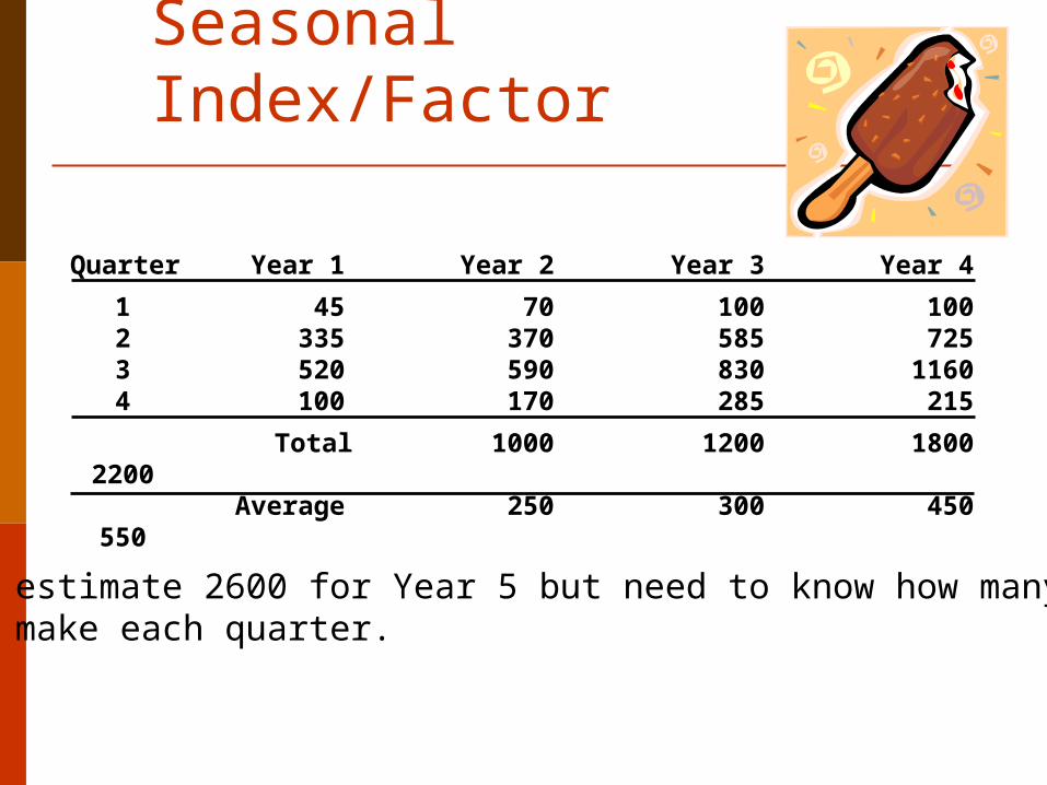
Quarter Year 1 Year 2 Year 3 Year 4
1 45 70 100 1002 335 370 585 7253 520 590 830 11604 100 170 285 215
Total 1000 1200 1800 2200 Average 250 300 450 550
Seasonal Index/Factor
We estimate 2600 for Year 5 but need to know how manyto make each quarter.

Seasonal Factor Method

Quarter Year 1 Year 2 Year 3 Year 4
1 45/250 = 0.18 70 100 1002 335 370 585 7253 520 590 830 11604 100 170 285 215
Total 1000 1200 1800 2200 Average 250 300 450 550
Seasonal Index = = 0.1845
250
Seasonal Index/Factor
Quarter Year 1 Year 2 Year 3 Year 4
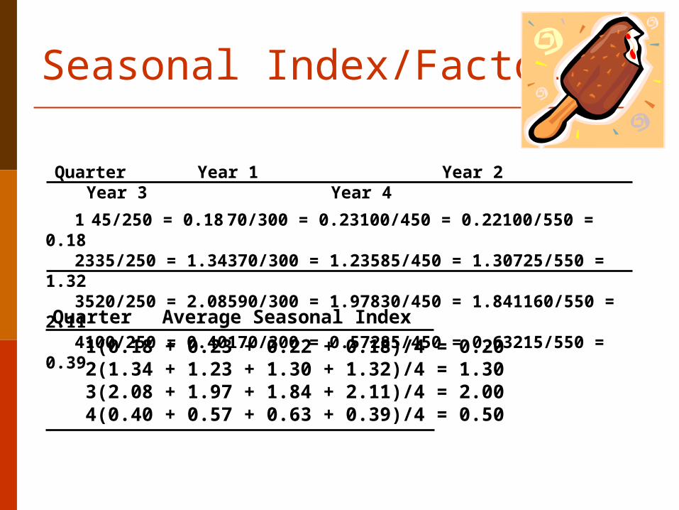
1 45/250 = 0.18 70/300 = 0.23 100/450 = 0.22 100/550 = 0.182 335/250 = 1.34 370/300 = 1.23 585/450 = 1.30 725/550 = 1.323 520/250 = 2.08 590/300 = 1.97 830/450 = 1.84 1160/550 = 2.114 100/250 = 0.40 170/300 = 0.57 285/450 = 0.63 215/550 = 0.39
Quarter Average Seasonal Index
1 (0.18 + 0.23 + 0.22 + 0.18)/4 = 0.202 (1.34 + 1.23 + 1.30 + 1.32)/4 = 1.303 (2.08 + 1.97 + 1.84 + 2.11)/4 = 2.004 (0.40 + 0.57 + 0.63 + 0.39)/4 = 0.50
Seasonal Index/Factor

Quarter Year 1 Year 2 Year 3 Year 4
1 45/250 = 0.18 70/300 = 0.23 100/450 = 0.22 100/550 = 0.182 335/250 = 1.34 370/300 = 1.23 585/450 = 1.30 725/550 = 1.323 520/250 = 2.08 590/300 = 1.97 830/450 = 1.84 1160/550 = 2.114 100/250 = 0.40 170/300 = 0.57 285/450 = 0.63 215/550 = 0.39
Quarter Average Seasonal Index Forecast
1 (0.18 + 0.23 + 0.22 + 0.18)/4 = 0.20 650(0.20) = 1302 (1.34 + 1.23 + 1.30 + 1.32)/4 = 1.30 650(1.30) = 8453 (2.08 + 1.97 + 1.84 + 2.11)/4 = 2.00 650(2.00) = 13004 (0.40 + 0.57 + 0.63 + 0.39)/4 = 0.50 650(0.50) = 325
Seasonal Influences

In- Class Problem: Forecast Year 3(Overall forecast = 1500)
Qtr
Year 1 Year 2Average
IndexDemand Index Demand Index
1 100 192
2 400 408
3 300 384
4 200 216
Avg

Decomposition of Season & Trend Decompose the data into components
Find seasonal component Deseasonalize demand Find Trend component
Forecast future values of each component Project Trend component into future Multiply trend component by seasonal
component

Example of Deseasonalized Data
Period x Quarter Actual Demand SF for X ASF DeseasonlizeAve SF Demand/ASF
1 I 600 0.47 0.74 809.912 II 1550 1.20 1.13 1376.693 III 1500 1.17 1.01 1479.914 IV 1500 1.17 1.12 1339.635 I 2400 0.87 0.74 3243.246 II 3100 1.13 1.13 2753.387 III 2600 0.95 1.01 2565.178 IV 2900 1.05 1.12 2589.969 I 3800 0.88 0.74 5135.1410 II 4500 1.05 1.13 3996.8411 III 4000 0.93 1.01 3946.4112 IV 4900 1.14 1.12 4376.13
Slope 338.4754Intercept 600.944
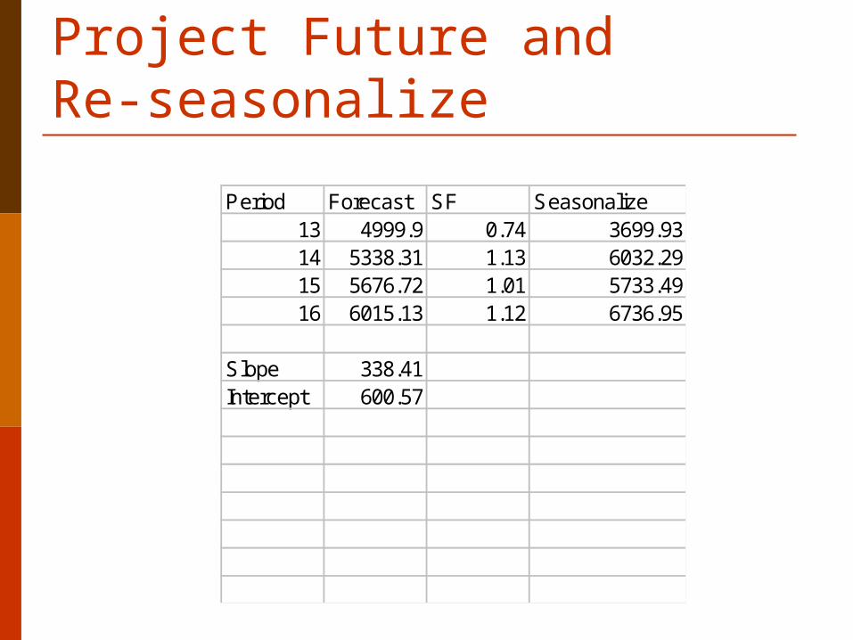
Project Future and Re-seasonalize
Period Forecast SF Seasonalize13 4999.9 0.74 3699.9314 5338.31 1.13 6032.2915 5676.72 1.01 5733.4916 6015.13 1.12 6736.95
Slope 338.41Intercept 600.57

Options for Brewery Case that use regression and/or seasonal adjustment? Using Yearly Data to
start? Using Monthly data to
start?

Trend-Adjusted Exponential Smoothing
| | | | | | | | | | | | | | |0 1 2 3 4 5 6 7 8 9 10 11 12 13 14 15
80 —
70 —
60 —
50 —
40 —
30 —
Gu
est
arr
ival
s
Week
Actual room requests

Trend-Adjusted Exponential Smoothing

Trend-Adjusted Exponential Smoothing
| | | | | | | | | | | | | | |0 1 2 3 4 5 6 7 8 9 10 11 12 13 14 15
80 —
70 —
60 —
50 —
40 —
30 —
Gu
est
arr
ival
s
Week
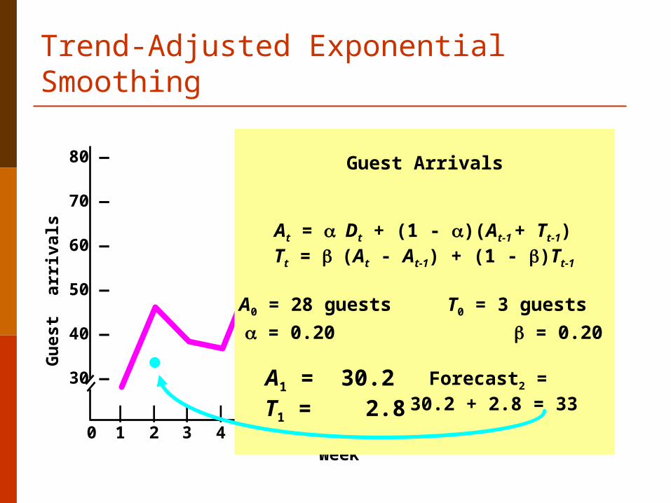
Guest Arrivals
At = Dt + (1 - )(At-1 + Tt-1)Tt = (At - At-1) + (1 - )Tt-1

Trend-Adjusted Exponential Smoothing
| | | | | | | | | | | | | | |0 1 2 3 4 5 6 7 8 9 10 11 12 13 14 15
80 —
70 —
60 —
50 —
40 —
30 —
Gu
est
arr
ival
s
Week
A1 = 0.2(27) + 0.80(28 + 3)= 30.2T1 = 0.2(30.2 - 28) + 0.80(3)= 2.8
Guest Arrivals
A0 = 28 g D1 = 27 g T0 = 3 g
= 0.20 = 0.20
At = Dt + (1 - )(At-1 + Tt-1)Tt = (At - At-1) + (1 - )Tt-1
Trend-Adjusted Exponential Smoothing
| | | | | | | | | | | | | | |0 1 2 3 4 5 6 7 8 9 10 11 12 13 14 15
80 —
70 —
60 —
50 —
40 —
30 —
Gu
est
arr
ival
s
Week
A1 = 30.2T1 = 2.8
Guest Arrivals
A0 = 28 guests T0 = 3 guests
= 0.20 = 0.20
At = Dt + (1 - )(At-1 + Tt-1)Tt = (At - At-1) + (1 - )Tt-1
Forecast2 = 30.2 + 2.8 = 33

Trend-Adjusted Exponential Smoothing
| | | | | | | | | | | | | | |0 1 2 3 4 5 6 7 8 9 10 11 12 13 14 15
80 —
70 —
60 —
50 —
40 —
30 —
Gu
est
arr
ival
s
Week
Guest Arrivals
A1 = 30.2 D2 = 44 T1 = 2.8
= 0.20 = 0.20
At = Dt + (1 - )(At-1 + Tt-1)Tt = (At - At-1) + (1 - )Tt-1
A2 =T2 =
Forecast =
Trend-Adjusted Exponential Smoothing
| | | | | | | | | | | | | | |0 1 2 3 4 5 6 7 8 9 10 11 12 13 14 15
80 —
70 —
60 —
50 —
40 —
30 —
Gu
est
arr
ival
s
Week
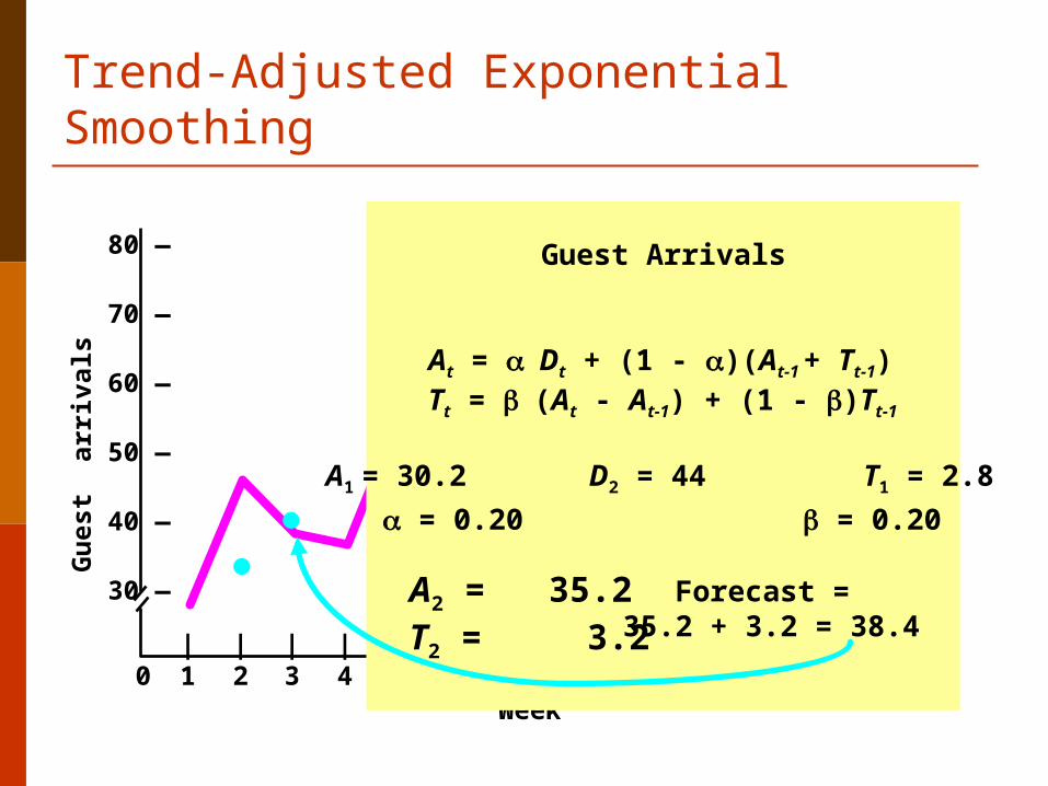
Guest Arrivals
A1 = 30.2 D2 = 44 T1 = 2.8
= 0.20 = 0.20
At = Dt + (1 - )(At-1 + Tt-1)Tt = (At - At-1) + (1 - )Tt-1
A2 = 35.2T2 = 3.2
Forecast = 35.2 + 3.2 = 38.4

Trend-Adjusted Exponential Smoothing
| | | | | | | | | | | | | | |0 1 2 3 4 5 6 7 8 9 10 11 12 13 14 15
80 —
70 —
60 —
50 —
40 —
30 —
Gu
est
arr
ival
s
Week
Trend-adjusted forecast
Actual guest arrivals

In Class Exercise
Amar = 300,000 cases; Tmar = +8,000 cases
Dapr = 330,000 cases; = 0.20 =.10
What are the forecasts for May and July?

The End


