Journal of Machine Learning Research 15 (2014) 1523-1548 Submitted 5/13; Revised 2/14; Published 4/14 Iteration Complexity of Feasible Descent Methods for Convex Optimization Po-Wei Wang [email protected]Chih-Jen Lin [email protected]Department of Computer Science National Taiwan University Taipei 106, Taiwan Editor: S. Sathiya Keerthi Abstract In many machine learning problems such as the dual form of SVM, the objective function to be minimized is convex but not strongly convex. This fact causes difficulties in obtaining the complexity of some commonly used optimization algorithms. In this paper, we proved the global linear convergence on a wide range of algorithms when they are applied to some non-strongly convex problems. In particular, we are the first to prove O(log(1/)) time complexity of cyclic coordinate descent methods on dual problems of support vector classification and regression. Keywords: convergence rate, convex optimization, iteration complexity, feasible descent methods 1. Introduction We consider the following convex optimization problem min x∈X f (x), where f (x) ≡ g(Ex)+ b > x, (1) where g(t) is a strongly convex function with Lipschitz continuous gradient, E is a constant matrix, and X is a polyhedral set. Many popular machine learning problems are of this type. For example, given training label-instance pairs (y i , z i ),i =1,...,l, the dual form of L1-loss linear SVM (Boser et al., 1992) is 1 min α 1 2 w > w - 1 T α subject to w = Eα, 0 ≤ α i ≤ C, i =1,...,l, (2) where E = y 1 z 1 ,...,y l z l , 1 is the vector of ones, and C is a given upper bound. Although w > w/2 is strongly convex in w, the objective function of (2) may not be strongly convex in α. Common optimization approaches for these machine learning problems include cyclic coordinate descent and others. Unfortunately, most existing results prove only local linear 1. Note that we omit the bias term in the SVM formulation. c 2014 Po-Wei Wang and Chih-Jen Lin.
Transcript
Journal of Machine Learning Research 15 (2014) 1523-1548 Submitted 5/13; Revised 2/14; Published 4/14
Iteration Complexity of Feasible Descent Methods forConvex Optimization
In many machine learning problems such as the dual form of SVM, the objective functionto be minimized is convex but not strongly convex. This fact causes difficulties in obtainingthe complexity of some commonly used optimization algorithms. In this paper, we provedthe global linear convergence on a wide range of algorithms when they are applied tosome non-strongly convex problems. In particular, we are the first to prove O(log(1/ε))time complexity of cyclic coordinate descent methods on dual problems of support vectorclassification and regression.
We consider the following convex optimization problem
minx∈X
f(x), where f(x) ≡ g(Ex) + b>x, (1)
where g(t) is a strongly convex function with Lipschitz continuous gradient, E is a constantmatrix, and X is a polyhedral set. Many popular machine learning problems are of thistype. For example, given training label-instance pairs (yi, zi), i = 1, . . . , l, the dual form ofL1-loss linear SVM (Boser et al., 1992) is1
minα
1
2w>w − 1Tα
subject to w = Eα, 0 ≤ αi ≤ C, i = 1, . . . , l,(2)
where E =[y1z1, . . . , ylzl
], 1 is the vector of ones, and C is a given upper bound. Although
w>w/2 is strongly convex in w, the objective function of (2) may not be strongly convexin α. Common optimization approaches for these machine learning problems include cycliccoordinate descent and others. Unfortunately, most existing results prove only local linear
1. Note that we omit the bias term in the SVM formulation.
convergence, so the number of total iterations cannot be calculated. One of the main diffi-culties is that f(x) may not be strongly convex. In this work, we establish the global linearconvergence for a wide range of algorithms for problem (1). In particular, we are the firstto prove that the popularly used cyclic coordinate descent methods for dual SVM problemsconverge linearly since the beginning. Many researchers have stated the importance of suchconvergence-rate analysis. For example, Nesterov (2012) said that it is “almost impossibleto estimate the rate of convergence” for general cases. Saha and Tewari (2013) also agreedthat “little is known about the non-asymptotic convergence” for cyclic coordinate descentmethods and they felt “this gap in the literature needs to be filled urgently.”
Luo and Tseng (1992a) are among the first to establish the asymptotic linear convergenceto a non-strongly convex problem related to (1). If X is a box (possibly unbounded)and a cyclic coordinate descent method is applied, they proved ε-optimality in O(r0 +log(1/ε)) time, where r0 is an unknown number. Subsequently, Luo and Tseng (1993)considered a class of feasible descent methods that broadly covers coordinate descent andgradient projection methods. For problems including (1), they proved the asymptotic linearconvergence. The key concept in their analysis is a local error bound, which states how closethe current solution is to the solution set compared with the norm of projected gradient∇+f(x).
minx∗∈X ∗
‖xr − x∗‖ ≤ κ‖∇+f(xr)‖, ∀r ≥ r0, (3)
where r0 is the above-mentioned unknown iteration index, X ∗ is the solution set of problem(1), κ is a positive constant, and xr is the solution produced after the r-th iteration. Becauser0 is unknown, we call (3) a local error bound, which only holds near the solution set. Localerror bounds have been used in other works for convergence analysis such as Luo and Tseng(1992b). If r0 = 0, we call (3) a global error bound from the beginning, and it may helpto obtain a global convergence rate. If f(x) is strongly convex and X is a polyhedral set,a global error bound has been established by Pang (1987, Theorem 3.1). One of the maincontributions of our work is to prove a global error bound of the possibly non-strongly convexproblem (1). Then we are able to establish the global linear convergence and O(log(1/ε))time complexity for the feasible descent methods.
We briefly discuss some related works, which differ from ours in certain aspects. Changet al. (2008) applied an (inexact) cyclic coordinate descent method for the primal problemof L2-loss SVM. Because the objective function is strongly convex, they are able to provethe linear convergence since the first iteration. Further, Beck and Tetruashvili (2013) estab-lished global linear convergence for block coordinate gradient descent methods on generalsmooth and strongly convex objective functions. Tseng and Yun (2009) applied a greedyversion of block coordinate descent methods on the non-smooth separable problems cov-ering the dual form of SVM. However, they proved only asymptotic linear convergenceand O(1/ε) complexity. Moreover, for large-scale linear SVM (i.e., kernels are not used),cyclic rather than greedy coordinate descent methods are more commonly used in practice.2
Wright (2012) considered the same non-smooth separable problems in Tseng and Yun (2009)and introduced a reduced-Newton acceleration that has asymptotic quadratic convergence.
2. It is now well known that greedy coordinate descent methods such as SMO (Platt, 1998) are less suitablefor linear SVM; see some detailed discussion in Hsieh et al. (2008, Section 4.1).
1524
Iteration Complexity of Feasible Descent Methods
For L1-regularized problems, Saha and Tewari (2013) proved O(1/ε) complexity for cycliccoordinate descent methods under a restrictive isotonic assumption.
Although this work focuses on deterministic algorithms, we briefly review past studieson stochastic (randomized) methods. An interesting fact is that there are more studieson the complexity of randomized rather than deterministic coordinate descent methods.Shalev-Shwartz and Tewari (2009) considered L1-regularized problems, and their stochasticcoordinate descent method converges in O(1/ε) iterations in expectation. Nesterov (2012)extended the settings to general convex objective functions and improved the iterationbound to O(1/
√ε) by proposing an accelerated method. For strongly convex function, he
proved that the randomized coordinate descent method converges linearly in expectation.Shalev-Shwartz and Zhang (2013a) provided a sub-linear convergence rate for a stochasticcoordinate ascent method, but they focused on the duality gap. Their work is interestingbecause it bounds the primal objective values. Shalev-Shwartz and Zhang (2013b) refinedthe sub-linear convergence to be O(min(1/ε, 1/
√ε)). Richtarik and Takac (2014) studied
randomized block coordinate descent methods for non-smooth convex problems and had sub-linear convergence on non-strongly convex functions. If the objective function is stronglyconvex and separable, they obtained linear convergence. Tappenden et al. (2013) extendedthe methods to inexact settings and had similar convergence rates to those in Richtarik andTakac (2014).
Our main contribution is a global error bound for the non-strongly convex problem(1), which ensures the global linear convergence of feasible descent methods. The maintheorems are presented in Section 2, followed by examples in Section 3. The global errorbound is discussed in Section 4, and the proof of global linear convergence of feasible descentmethods is given in Section 5. We conclude in Section 6 while leaving properties of projectedgradients in Appendix A.
2. Main Results
Consider the general convex optimization problem
minx∈X
f(x), (4)
where f(x) is proper convex and X is nonempty, closed, and convex. We will prove globallinear convergence for a class of optimization algorithms if problem (4) satisfies one of thefollowing assumptions.
Assumption 2.1 f(x) is σ strongly convex and its gradient is ρ Lipschitz continuous.That is, there are constants σ > 0 and ρ such that
σ‖x1 − x2‖2 ≤ (∇f(x1)−∇f(x2))>(x1 − x2), ∀x1,x2 ∈ X
and‖∇f(x1)−∇f(x2)‖ ≤ ρ‖x1 − x2‖, ∀x1,x2 ∈ X .
Assumption 2.2 X = {x | Ax ≤ d} is a polyhedral set, the optimal solution set X ∗ isnon-empty, and
f(x) = g(Ex) + b>x, (5)
1525
Wang and Lin
where g(t) is σg strongly convex and ∇f(x) is ρ Lipschitz continuous. This assumptioncorresponds to problem (1) that motivates this work.
The optimal set X ∗ under Assumption 2.1 is non-empty following Weierstrass extreme valuetheorem.3 Subsequently, we make several definitions before presenting the main theorem.
Definition 2.3 (Convex Projection Operator)
[x]+X ≡ arg miny∈X‖x− y‖.
From Weierstrass extreme value theorem and the strong convexity of ‖x − y‖2 to y, theunique [x]+X exists for any X that is closed, convex, and non-empty.
Definition 2.4 (Nearest Optimal Solution)
x ≡ [x]+X ∗ .
With this definition, minx∗∈X ∗ ‖x− x∗‖ could be simplified to ‖x− x‖.
Definition 2.5 (Projected Gradient)
∇+f(x) ≡ x− [x−∇f(x)]+X .
As shown in Lemma A.6, the projected gradient is zero if and only if x is an optimalsolution. Therefore, it can be used to check the optimality. Further, we can employ theprojected gradient to define an error bound, which measures the distance between x andthe optimal set; see the following definition.
Definition 2.6 An optimization problem admits a global error bound if there is a con-stant κ such that
‖x− x‖ ≤ κ‖∇+f(x)‖, ∀x ∈ X . (6)
A relaxed condition called global error bound from the beginning if the above inequalityholds only for x satisfying
x ∈ X and f(x)− f(x) ≤M,
where M is a constant. Usually, we have
M ≡ f(x0)− f∗,
where x0 is the start point of an optimization algorithm and f∗ is the optimal functionvalue. Therefore, we called this as a bound “from the beginning.”
3. The strong convexity in Assumption 2.1 implies that the sublevel set is bounded (Vial, 1983). ThenWeierstrass extreme value theorem can be applied.
1526
Iteration Complexity of Feasible Descent Methods
The global error bound is a property of the optimization problem and is independent fromthe algorithms. If a bound holds,4 then using Lemmas A.5, A.6, and (6) we can obtain
1
2 + ρ‖∇+f(x)‖ ≤ ‖x− x‖ ≤ κ‖∇+f(x)‖, ∀x ∈ X .
This property indicates that ‖∇+f(x)‖ is useful to estimate the distance to the optimum.We will show that a global error bound enables the proof of global linear convergence ofsome optimization algorithms. The bound under Assumption 2.1, which requires strongconvexity, was already proved in Pang (1987) with
κ =1 + ρ
σ.
However, for problems under Assumption 2.2 such as the dual form of L1-loss SVM, theobjective function is not strongly convex, so a new error bound is required. We prove thebound in Section 4 with
κ = θ2(1 + ρ)(1 + 2‖∇g(t∗)‖2
σg+ 4M) + 2θ‖∇f(x)‖, (7)
where t∗ is a constant vector that equals Ex∗, ∀x∗ ∈ X ∗ and θ is the constant fromHoffman’s bound (Hoffman, 1952; Li, 1994).
θ ≡ supu,v
∥∥∥∥uv∥∥∥∥∣∣∣∣∣∣∣‖A>u+
(Eb>)>v‖ = 1, u ≥ 0.
The corresponding rows of A, E to u, v’s
non-zero elements are linearly independent.
.
Specially, when b = 0 or X = Rl, the constant could be simplified to
κ = θ21 + ρ
σg. (8)
Now we define a class of optimization algorithms called the feasible descent methods forsolving (4).
Definition 2.7 (Feasible Descent Methods) A sequence {xr} is generated by a feasibledescent method if for every iteration index r, {xr} satisfies
xr+1 = [xr − ωr∇f(xr) + er]+X , (9)
‖er‖ ≤ β‖xr − xr+1‖ , (10)
f(xr)− f(xr+1) ≥ γ‖xr − xr+1‖2, (11)
where infr ωr > 0, β > 0, and γ > 0.
4. Note that not all problems have a global error bound. An example is minx∈R x4.
1527
Wang and Lin
The framework of feasible descent methods broadly covers many algorithms that use thefirst-order information. For example, the projected gradient descent, the cyclic coordinatedescent, the proximal point minimization, the extragradient descent, and matrix splittingalgorithms are all feasible descent methods (Luo and Tseng, 1993). With the global errorbound under Assumption 2.1 or Assumption 2.2, in the following theorem we prove theglobal linear convergence for all algorithms that fit into the feasible descent methods.
Theorem 2.8 (Global Linear Convergence) If an optimization problem satisfies As-sumption 2.1 or 2.2, then any feasible descent method on it has global linear convergence.To be specific, the method converges Q-linearly with
f(xr+1)− f∗ ≤ φ
φ+ γ(f(xr)− f∗), ∀r ≥ 0,
where κ is the error bound constant in (6),
φ = (ρ+1 + β
ω)(1 + κ
1 + β
ω), and ω ≡ min(1, inf
rωr).
This theorem enables global linear convergence in many machine learning problems. Theproof is given in Section 5. In Section 3, we discuss examples on cyclic coordinate descentmethods.
3. Examples: Cyclic Coordinate Descent Methods
Cyclic coordinate descent methods are now widely used for machine learning problemsbecause of its efficiency and simplicity (solving a one-variable sub-problem at a time). Luoand Tseng (1992a) proved the asymptotic linear convergence if sub-problems are solvedexactly, and here we further show the global linear convergence.
3.1 Exact Cyclic Coordinate Descent Methods for Dual SVM Problems
In the following algorithm, each one-variable sub-problem is exactly solved.
Definition 3.1 A cyclic coordinate descent method on a box X = X1 × · · · × Xl is definedby the update rule
xr+1i = arg min
xi∈Xi
f(xr+11 , . . . , xr+1
i−1 , xi, xri+1, . . . , x
rl ), for i = 1, . . . , l, (12)
where Xi is the region under box constraints for coordinate i.
The following lemma shows that coordinate descent methods are special cases of the feasibledescent methods.
Lemma 3.2 The cyclic coordinate descent method is a feasible descent method with
ωr = 1, ∀r, β = 1 + ρ√l,
and
γ =
{σ2 if Assumption 2.1 holds,12 mini ‖Ei‖2 if Assumption 2.2 holds with ‖Ei‖ > 0, ∀i,
where Ei is the ith column of E.
1528
Iteration Complexity of Feasible Descent Methods
Proof This lemma can be directly obtained using Proposition 3.4 of Luo and Tseng (1993).Our assumptions correspond to cases (a) and (c) in Theorem 2.1 of Luo and Tseng (1993),which fulfill conditions needed by their Proposition 3.4.
For faster convergence, we may randomly permute all variables before each cycle of updatingthem (e.g., Hsieh et al., 2008). This setting does not affect the proof of Lemma 3.2.
Theorem 2.8 and Lemma 3.2 immediately imply the following corollary.
Corollary 3.3 The cyclic coordinate descent methods have global linear convergence if As-sumption 2.1 is satisfied or Assumption 2.2 is satisfied with ‖Ei‖ > 0, ∀i.
Next, we analyze the cyclic coordinate descent method to solve dual SVM problems. Themethod can be traced back to Hildreth (1957) for quadratic programming problems andhas recently been widely used following the work by Hsieh et al. (2008). For L1-loss SVM,we have shown in (2) that the objective function can be written in the form of (1) by astrongly convex function g(w) = w>w/2 and Ei = yizi for all label-instance pair (yi, zi).Hsieh et al. (2008) pointed out that ‖Ei‖ = 0 implies the optimal α∗i is C, which can beobtained at the first iteration and is never changed. Therefore, we need not consider suchvariables at all. With all conditions satisfied, Corollary 3.3 implies that cyclic coordinatedescent method for dual L1-loss SVM has global linear convergence. For dual L2-loss SVM,the objective function is
1
2α>Qα− 1>α+
1
2Cα>α, (13)
where Qt,j = ytyjz>t zj ,∀1 ≤ t, j ≤ l and 1 is the vector of ones. Eq. (13) is strongly convex
and its gradient is Lipschitz continuous, so Assumption 2.1 and Corollary 3.3 imply theglobal linear convergence.
We move on to check the dual problems of support vector regression (SVR). Given value-instance pairs (yi, zi), i = 1, . . . , l, the dual form of L1-loss m-insensitive SVR (Vapnik,1995) is
minα
1
2α>[Q −Q−Q Q
]α+
[m1− ym1 + y
]>α (14)
subject to 0 ≤ αi ≤ C, i = 1, . . . , 2l,
where Qt,j = z>t zj , ∀1 ≤ t, j ≤ l, and m and C are given parameters. Similar to the caseof classification, we can also perform cyclic coordinate descent methods; see Ho and Lin(2012, Section 3.2). Note that Assumption 2.2 must be used here because for any Q, theHessian in (14) is only positive semi-definite rather than positive definite. In contrast, forclassification, if Q is positive definite, the objective function in (2) is strongly convex andAssumption 2.1 can be applied. To represent (14) in the form of (1), let
Ei = zi, i = 1, . . . , l and Ei = −zi, i = l + 1, . . . , 2l.
Then g(w) = w>w/2 with w = Eα is a strongly convex function to w. Similar to thesituation in classification, if ‖Ei‖ = 0, then the optimal α∗i is bounded and can be obtainedat the first iteration. Without considering these variables, Corollary 3.3 implies the globallinear convergence.
1529
Wang and Lin
3.2 Inexact Cyclic Coordinate Descent Methods for Primal SVM Problems
In some situations the sub-problems (12) of cyclic coordinate descent methods cannot beeasily solved. For example, in Chang et al. (2008) to solve the primal form of L2-loss SVM,
minw
f(w), where f(w) ≡ 1
2w>w + C
l∑i=1
max(1− yiw>zi, 0)2, (15)
each sub-problem does not have a closed-form solution, and they approximately solve thesub-problem until a sufficient decrease condition is satisfied. They have established theglobal linear convergence, but we further show that their method can be included in ourframework.
To see that Chang et al. (2008)’s method is a feasible descent method, it is sufficientto prove that (9)-(11) hold. First, we notice that their sufficient decrease condition forupdating each variable can be accumulated. Thus, for one cycle of updating all variables,we have
f(wr)− f(wr+1) ≥ γ‖wr −wr+1‖2,
where γ > 0 is a constant. Next, because (15) is unconstrained, if zi ∈ Rn,∀i, we can make
X = Rn and er = wr+1 −wr +∇f(wr)
such that
wr+1 = [wr −∇f(wr) + er]+X .
Finally, from Appendix A.3 of Chang et al. (2008),
‖er‖ ≤ ‖wr −wr+1‖+ ‖∇f(wr)‖ ≤ β‖wr −wr+1‖,
where β > 0 is a constant. Therefore, all conditions (9)-(11) hold. Note that (15) is stronglyconvex because of the w>w term and ∇f(w) is Lipschitz continuous from (Lin et al., 2008,Section 6.1), so Assumption 2.1 is satisfied. With Theorem 2.8, the method by Chang et al.(2008) has global linear convergence.
3.3 Gauss-Seidel Methods for Solving Linear Systems
Gauss-Seidel (Seidel, 1874) is a classic iterative method to solve a linear system
Qα = b. (16)
Gauss-Seidel iterations take the following form.
αr+1i =
bi −∑i−1
j=1Qijαr+1j −
∑lj=i+1Qijα
rj
Qii. (17)
If Q is symmetric positive semi-definite and (16) has at least one solution, then the followingoptimization problem
minα∈Rl
1
2α>Qα− b>α (18)
1530
Iteration Complexity of Feasible Descent Methods
has the same solution set as (16). Further, αr+1i in (17) is the solution of minimizing
(18) over αi while fixing αr+11 , . . . , αr+1
i−1 , αri+1, . . . , α
rl . Therefore, Gauss-Seidel method is a
special case of coordinate descent methods.
Clearly, we need Qii > 0,∀i so that (17) is well defined. This condition also implies that
Q = E>E, where E has no zero column. (19)
Otherwise, ‖Ei‖ = 0 leads to Qii = 0 so the Qii > 0 assumption is violated. Note thatbecause Q is symmetric positive semi-definite, its orthogonal diagonalization UTDU existsand we choose E =
√DU . Using (19) and Lemma 3.2, Gauss-Seidel method is a feasible
descent method. By Assumption 2.2 and our main Theorem 2.8, we have the followingconvergence result.
Corollary 3.4 If
1. Q is symmetric positive semi-definite and Qii > 0, ∀i, and
2. The linear system (16) has at least a solution,
then the Gauss-Seidel method has global linear convergence.
This corollary covers some well-known results of the Gauss-Seidel method, which werepreviously proved by other ways. For example, in most numerical linear algebra textbooks(e.g., Golub and Van Loan, 1996), it is proved that if Q is strictly diagonally dominant(i.e., Qii >
∑j 6=i |Qij |, ∀i), then the Gauss-Seidel method converges linearly. We show in
Lemma C.1 that a strictly diagonally dominant matrix is positive definite, so Corollary 3.4immediately implies global linear convergence.
3.4 Quantity of the Convergence Rate
To demonstrate the relationship between problem parameters (e.g., number of instancesand features) and the convergence rate constants, we analyze the constants κ and φ fortwo problems. The first example is the exact cyclic coordinate descent method for the dualproblem (2) of L1-loss SVM. For simplicity, we assume ‖Ei‖ = 1, ∀i, where Ei denotes theith column of E. We have
σg = 1 (20)
by g(t) = t>t/2. Observe the following primal formulation of L1-loss SVM.
minw
P (w), where P (w) ≡ 1
2w>w + C
l∑i=1
max(1− yiw>zi, 0).
Let w∗ and α∗ be any optimal solution of the primal and the dual problems, respectively.By KKT optimality condition, we have w∗ = Eα∗. Consider α0 = 0 as the initial feasiblesolution. With the duality and the strictly decreasing property of {f(αr)},
2w∗>w∗ ≤ P (w∗) ≤ P (0) ≤ Cl implies ‖w∗‖ = ‖Eα∗‖ ≤
√2Cl. (22)
From (22),
‖∇f(α)‖ ≤ ‖E‖‖Eα∗‖+ ‖1‖ ≤√
Σi‖Ei‖2‖Eα∗‖+ ‖1‖ ≤√
2Cl +√l. (23)
To conclude, by (7), (20), (21), (22), (23), and ∇g(w∗) = w∗,
κ = θ2(1 + ρ)(1 + 2‖∇g(w∗)‖2
σg+ 4M) + 2θ‖∇f(α)‖
≤ θ2(1 + ρ)((1 + 4Cl) + 4Cl) + 2θ(√
2Cl +√l)
= O(ρθ2Cl).
Now we examine the rate φ for linear convergence. From Theorem 2.8, we have
φ = (ρ+1 + β
ω)(1 + κ
1 + β
ω)
= (ρ+ 2 + ρ√l)(1 + κ(2 + ρ
√l))
= O(ρ3θ2Cl2),
where
ω = 1, β = 1 + ρ√l, γ =
1
2(24)
are from Lemma 3.2 and the assumption that ‖Ei‖ = 1, ∀i. To conclude, we have κ =O(ρθ2Cl) and φ = O(ρ3θ2Cl2) for the exact cyclic coordinate descent method for the dualproblem of L1-loss SVM.
Next we consider the Gauss-Seidel method for solving linear systems in Section 3.3 byassuming ‖Q‖ = 1 and Qii > 0, ∀i, where ‖Q‖ denotes the spectral norm of Q. Similar to(20), we have σg = 1 by g(t) = t>t/2. Further, ρ = 1 from
‖∇f(α1)−∇f(α2)‖ ≤ ‖Q‖‖α1 −α2‖ = ‖α1 −α2‖.
Because the optimization problem is unconstrained, by (8) we have
κ = θ21 + ρ
σg= 2θ2, (25)
where θ is defined as
θ ≡ supv
‖v‖∣∣∣∣∣∣∣‖E>v‖ = 1.
The corresponding rows of E to v’s
non-zero elements are linearly independent.
, (26)
and E =√DU is from the orthogonal diagonalization of Q in (19). To have that the
corresponding rows of E to v’s non-zero elements are linearly independent, we need
vi = 0 if Dii = 0.
1532
Iteration Complexity of Feasible Descent Methods
Therefore, problem (26) becomes to select vi with Dii > 0 such that E>v = 1 and ‖v‖ ismaximized. Because U ’s rows are orthogonal vectors and any Dii > 0 is an eigen-value ofQ, the maximum occurs if we choose ν = ei as the indicator vector corresponding to thesmallest non-zero eigen-value σmin -nnz. Then,
the solution v in (26) isν
√σmin -nnz
and θ2 =1
σmin -nnz. (27)
From Lemma 3.2, ω, β, and γ of the Gauss-Seidel method are the same as (24). Thus,Theorem 2.8, (24), (25), and (27) give the convergence rate constant
φ = (3 +√l)(1 + κ(2 +
√l)) = (3 +
√l)(1 +
4 + 2√l
σmin -nnz). (28)
With (24), (28), and Theorem 2.8, the Gauss-Seidel method on solving linear systems haslinear convergence with
f(αr+1)− f∗ ≤ (1− σmin -nnz
4(6 + 5√l + l) + (7 + 2
√l)σmin -nnz)
)(f(αr)− f∗), ∀r ≥ 0.
We discuss some related results. A similar rate of linear convergence appears in Beck andTetruashvili (2013). They assumed f is σmin strongly convex and the optimization problemis unconstrained. By considering a block coordinate descent method with a conservativerule of selecting the step size, they showed
f(αr+1)− f∗ ≤ (1− σmin
2(1 + l))(f(αr)− f∗), ∀r ≥ 0.
Our obtained rate is comparable, but is more general to cover singular Q.
4. Proofs of Global Error Bounds
In this section, we prove the global error bound (6) under Assumptions 2.1 or 2.2. Thefollowing theorem proves the global error bound under Assumption 2.1.
Theorem 4.1 (Pang 1987, Theorem 3.1) Under Assumption 2.1,
‖x− x‖ ≤ κ‖∇+f(x)‖, ∀x ∈ X ,
where κ = (1 + ρ)/σ.
Proof Because f(x) is strongly convex, X ∗ has only one element x. From Lemmas A.4and A.6, the result holds immediately.
The rest of this section focuses on proving a global error bound under Assumption 2.2.We start by sketching the proof. First, observe that the optimal set is a polyhedron byLemma 4.2. Then ‖x − x‖ is identical to the distance of x to the polyhedron. A knowntechnique to bound the distance between x and a polyhedron is Hoffman’s bound (Hoffman,
1533
Wang and Lin
1952). Because the original work uses L1-norm, we provide in Lemma 4.3 a special versionof Li (1994) that uses L2-norm. With the feasibility of x, there is
‖x− x‖ ≤ θ(A,(Eb>)) ∥∥∥∥E(x− x)
b>(x− x)
∥∥∥∥ ,where θ
(A,(Eb>))
is a constant related to A, E, and b. Subsequently, we bound ‖E(x−x)‖2
and (b>(x − x))2 in Lemmas 4.4 and 4.5 by values consisting of ‖∇+f(x)‖ and ‖x − x‖.Such bounds are obtained using properties of the optimization problem such as the strongconvexity of g(·). Finally, we obtain a quadratic inequality involving ‖∇+f(x)‖ and ‖x−x‖,which eventually leads to a global error bound under Assumption 2.2.
We begin the formal proof by expressing the optimal set as a polyhedron.
Lemma 4.2 (Optimal Condition) Under Assumption 2.2, there are unique t∗ and s∗
such that ∀x∗ ∈ X ∗,Ex∗ = t∗, b>x∗ = s∗, and Ax∗ ≤ d. (29)
Note that A and d are the constants for generating the feasible set X = {x | Ax ≤ d}.Further,
x∗ satisfies (29)⇔ x∗ ∈ X ∗. (30)
Specially, when b = 0 or X = Rl,5
Ex∗ = t∗, Ax∗ ≤ d⇔ x∗ ∈ X ∗. (31)
Proof First, we prove (29). The proof is similar to Lemma 3.1 in Luo and Tseng (1992a).For any x∗1,x
∗2 ∈ X ∗, from the convexity of f(x),
f((x∗1 + x∗2)/2) = (f(x∗1) + f(x∗2))/2.
By the definition of f(x) in Assumption 2.2, we have
Cancel b>(x∗1+x∗2)/2 from both sides. By the strong convexity of g(t), we have Ex∗1 = Ex∗2.Thus, t∗ ≡ Ex∗ is unique. Similarly, because f(x∗1) = f(x∗2),
g(t∗) + b>x∗1 = g(t∗) + b>x∗2.
Therefore, s∗ ≡ b>x∗ is unique, and Ax∗ ≤ d, ∀x∗ ∈ X ∗ holds naturally by X ∗ ⊆ X .Further,
f(x∗) = g(t∗) + s∗, ∀x∗ ∈ X ∗. (32)
The result in (29) immediately implies the (⇐) direction of (30). For the (⇒) direction,for any x∗ satisfying
Ex∗ = t∗, b>x∗ = s∗, Ax∗ ≤ d,
we have f(x∗) = g(t∗) + s∗. From (32), x∗ is an optimal solution.
5. When X = Rl, we can take zero A and d for a trivial linear inequality.
1534
Iteration Complexity of Feasible Descent Methods
Now we examine the special cases. If b = 0, we have b>x = 0, ∀x ∈ X . Therefore, (30)is reduced to (31). On the other hand, if X = Rl, the optimization problem is unconstrained.Thus,
x∗ is optimal⇔ ∇f(x∗) = 0 = E>∇g(t∗) + b.
As a result, Ex∗ = t∗ is a necessary and sufficient optimality condition.
Because the optimal set is a polyhedron, we will apply the following Hoffman’s boundin Lemma 4.6 to upper-bound the distance to the optimal set by the violation of the poly-hedron’s linear inequalities.
Lemma 4.3 (Hoffman’s Bound) Let P be the non-negative orthant and consider a non-empty polyhedron
{x∗ | Ax∗ ≤ d, Ex∗ = t}.
For any x, there is a feasible point x∗ such that
‖x− x∗‖ ≤ θ(A,E)
∥∥∥∥[Ax− d]+PEx− t
∥∥∥∥ , (33)
where
θ(A,E) ≡ supu,v
∥∥∥∥uv∥∥∥∥∣∣∣∣∣∣∣‖A>u+ E>v‖ = 1, u ≥ 0.
The corresponding rows of A, E to u, v’s
non-zero elements are linearly independent.
. (34)
Note that θ(A,E) is independent of x.
The proof of the lemma is given in Appendix B. Before applying Hoffman’s bound, we needsome technical lemmas to bound ‖Ex − t∗‖2 and (b>x − s∗)2, which will appear on theright-hand side of Hoffman’s bound for the polyhedron of the optimal set.
Lemma 4.4 Under Assumption 2.2, we have constants ρ and σg such that
‖Ex− t∗‖2 ≤ 1 + ρ
σg‖∇+f(x)‖‖x− x‖, ∀x ∈ X .
Proof By Ex = t∗ from Lemma 4.2, the strong convexity of g(t), and the definition off(x) in (5), there exists σg such that
Consider the right-hand side in (36). The second term can be bounded by 2‖∇g(t∗)‖2‖Ex−t∗‖2, and the first term is bounded using the inequalities
∇f(x)>(x− x) ≤ ∇f(x)>(x− x)
≤ ∇+f(x)>(x− x+∇f(x)−∇+f(x))
≤ ∇+f(x)>(x− x+∇f(x)−∇f(x) +∇f(x))
≤ (1 + ρ)‖∇+f(x)‖‖x− x‖+∇+f(x)>∇f(x). (37)
The first inequality is by convexity, the second is by Lemma A.1,6 the third is by ‖∇+f(x)‖2 ≥0, and the last is by the Lipschitz continuity of ∇f . By the optimality of x,
∇f(x)>([x−∇f(x)]+X − x+ x− x) ≥ 0. (38)
Thus, (38), the convexity of f(·), and (35) imply that
∇f(x)>∇+f(x) ≤ ∇f(x)>(x− x) ≤ f(x)− f(x) ≤M. (39)
Leta ≡ ∇f(x)>(x− x), u ≡ (1 + ρ)‖∇+f(x)‖‖x− x‖, v ≡ ∇f(x)>∇+f(x).
Then we have
0 ≤ a ≤ u+ v from (37) and optimality of x, a− v ≥ 0 from (39), and u ≥ 0.
Therefore, a2 ≤ au+ av ≤ au+ v(u+ v) ≤ au+ au+ v2 ≤ 2au+ 2v2, and
With Lemmas 4.4 and 4.5, if f(x)− f∗ ≤M , we can bound ‖Ex− t∗‖2 and (b>x− s∗)2 toobtain
‖x− x‖2
≤ θ2(1 + ρ)(1 + 2‖∇g(t∗)‖2
σg+ 4M)‖∇+f(x)‖‖x− x‖+ 4θ2‖∇f(x)‖2‖∇+f(x)‖2.
(41)
Leta ≡ ‖x− x‖, c ≡ 2θ‖∇f(x)‖‖∇+f(x)‖, and
b ≡ θ2(1 + ρ)(1 + 2‖∇g(t∗)‖2
σg+ 4M)‖∇+f(x)‖.
(42)
Then we can rewrite (41) as
a2 ≤ ba+ c2 with a ≥ 0, b ≥ 0, c ≥ 0. (43)
We claim thata ≤ b+ c. (44)
Otherwise, a > b+ c implies that
a2 > a(b+ c) > ba+ c2,
1537
Wang and Lin
a violation to (43). By (42) and (44), the proof is complete.Now we examine the special case of b = 0 or X = Rl. From (31) in Lemma 4.2, we can
apply Lemma 4.3 to have the existence of θ(A,E) such that ∀x ∈ X , there is x∗ ∈ X ∗ sothat
‖x− x‖ ≤ ‖x− x∗‖ ≤ θ(A,E)‖Ex− t∗‖.With Lemma 4.4, we have
‖x− x‖2 ≤ θ(A,E)21 + ρ
σg‖∇+f(x)‖‖x− x‖.
After canceling ‖x− x‖ from both sides, the proof is complete.
5. Proof of Theorem 2.8
The proof is modified from Theorem 3.1 of Luo and Tseng (1993). They applied a localerror bound to obtain asymptotic local linear convergence, while ours applies a global errorbound to have linear convergence from the first iteration.
Because f(x) is convex, f(xr), ∀r correspond to the same unique optimal function value.Thus the global linear convergence is established.
6. Discussions and Conclusions
For future research, we plan to extend the analysis to other types of algorithms and problems(e.g., L1-regularized problems). Further, the global error bound will be useful in analyzingstopping criteria and the effect of parameter changes on the running time of machine learningproblems (for example, the change of parameter C in SVM).
In conclusion, by focusing on a convex but non-strongly convex problem (1), we estab-lished a global error bound. We then proved the global linear convergence on a wide rangeof deterministic algorithms, including cyclic coordinate descent methods for dual SVM andSVR. Consequently, the time complexity of these algorithms is O(log(1/ε)).
Acknowledgments
This work was supported in part by the National Science Council of Taiwan via the grant101-2221-E-002-199-MY3. The authors thank associate editor and anonymous reviewers forvaluable comments. We also thank Pinghua Gong for pointing out a mistake in the proofof Lemma 4.5, and Lijun Zhang for a mistake in Section 3.4.
Appendix A. Properties of Projected Gradient
We present some properties of projected gradient used in the proofs. Most of them areknown in the literature, but we list them here for completeness. Throughout this section,we assume X is a non-empty, closed, and convex set.
First, we present a fundamental result used in the paper: the projection theorem to anon-empty closed convex set X . The convex projection in Definition 2.3 is equivalent tothe following inequality on the right-hand side of (51). That is, if the inequality holds forany z, this z will be the result of the convex projection and vise versa.
Lemma A.1 (Projection Theorem)
z = [x]+X ⇔ (z − x)>(z − y) ≤ 0, ∀y ∈ X . (51)
1539
Wang and Lin
Proof The proof is modified from Hiriart-Urruty and Lemarechal (2001, Theorem 3.1.1).From the convexity of X ,
Divide α from both sides, and let α ↓ 0. Then we have (⇒).For (⇐), if z = x, then 0 = ‖z − x‖ ≤ ‖y − x‖ holds for all y ∈ X . Thus, z = [x]+X . If
z 6= x, then for any y ∈ X ,
0 ≥ (z − x)>(z − y) = ‖x− z‖2 + (y − x)>(x− z)
≥ ‖x− z‖2 − ‖x− y‖‖x− z‖.
Divide ‖x− z‖ > 0 from both sides. Because the inequality is valid for all y, (⇐) holds.
The following lemma shows that the projection operator is Lipschitz continuous.
Lemma A.2 (Lipschitz Continuity of Convex Projection)
‖[x]+X − [y]+X ‖ ≤ ‖x− y‖, ∀x,y.
Proof The proof is modified from Hiriart-Urruty and Lemarechal (2001) Proposition 3.1.3.Let u = [x]+X and v = [y]+X . If u = v, then the result holds immediately. If not, with
Lemma A.1 we have
(u− x)>(u− v) ≤ 0, (52)
(v − y)>(v − u) ≤ 0. (53)
Summing (52) and (53), we have
(u− v)>(u− x− v + y) ≤ 0.
We could rewrite it as
‖u− v‖2 ≤ (u− v)>(x− y) ≤ ‖u− v‖‖x− y‖.
Cancel ‖u− v‖ > 0 at both sides. Then the result holds.
Lemma A.3 Assume ∇f(x) is ρ Lipschitz continuous. Then ∀x,y ∈ X ,
where the first and the last inequalities are from (58) and (59), respectively, and the secondinequality is from ([u]+X−[v]+X )>z = z>z ≥ 0. With 0 < α1 < α2, (60) implies∇f(x)>z ≥ 0and
(x− [u]+X )>z ≥ 0.
Using this inequality,
‖x− [v]+X ‖2 = ‖x− [u]+X + z‖2 = ‖x− [u]+X ‖
2 + 2(x− [u]+X )>z + ‖z‖2 ≥ ‖x− [u]+X ‖2.
Therefore, from (56)-(57),
‖x− [x− α2∇f(x)]+X ‖ ≥ ‖x− [x− α1∇f(x)]+X ‖.
With 0 < α1 < α2, the proof is complete.
Lemma A.8 ∀x ∈ X and α > 0, if
u = x− [x−∇f(x)]+X ,
v = x− [x− α∇f(x)]+X ,
thenmin(1, α)‖u‖ ≤ ‖v‖ ≤ max(1, α)‖u‖.
Proof From Lemma 1 in Gafni and Bertsekas (1984), ‖x − [x − α∇f(x)]+X ‖/α is mono-tonically decreasing for all α > 0. Thus,
α‖x− [x−∇f(x)]+X ‖ ≤ ‖x− [x− α∇f(x)]+X ‖, ∀α ≤ 1.
From Lemma A.7, we have
‖x− [x−∇f(x)]+X ‖ ≤ ‖x− [x− α∇f(x)]+X ‖, ∀α ≥ 1.
Therefore, min(1, α)‖u‖ ≤ ‖v‖. A similar proof applies to ‖v‖ ≤ max(1, α)‖u‖.
Appendix B. Proof of Hoffman’s Bound (Lemma 4.3)
The following proof is a special case of Mangasarian and Shiau (1987) and Li (1994), whichbounds the distance of a point to the polyhedron by the violation of inequalities. We beginwith an elementary theorem in convex analysis.
Lemma B.1 (Caratheodory’s Theorem) For a non-empty polyhedron
A>u+ E>v = y, u ≥ 0, (61)
there is a feasible point (u,v) such that
The corresponding rows of A, E to u, v’s non-zero elements are linearly independent.(62)
1543
Wang and Lin
Proof Let (u,v) be a point in the polyhedron, and therefore E>v = y − A>u. If thecorresponding rows of E to non-zero elements of v are not linearly independent, we canmodify v so that E>v remains the same and E’s rows corresponding to v’s non-zero elementsare linearly independent. Thus, without loss of generality, we assume that E is full row-rank. Denote a>i as the ith row of A and e>j as the jth row of E. If the corresponding rowsof A,E to non-zero elements of u,v are not linearly independent, there exists (λ, ξ) suchthat
1. (λ, ξ) 6= 0.
2. (λ, ξ)’s non-zero elements correspond to the non-zero elements of (u,v). That is,λi = 0 if ui = 0, ∀i, and ξj = 0 if vj = 0, ∀j.
3. (λ, ξ) satisfies ∑i: ui>0, λi 6=0
λiai +∑
j: vj 6=0, ξj 6=0
ξjej = 0.
Besides, the set {i | ui > 0, λi 6= 0} is not empty because the rows of E are linearlyindependent. Otherwise, a contradiction occurs from λ = 0, ξ 6= 0, and∑
j: vj 6=0, ξj 6=0
ξiej = 0.
By choosing
s = mini: ui>0, λi 6=0
uiλi> 0,
we have
A>(u− sλ) + E>(v − sξ) = A>u+ E>v = y and u− sλ ≥ 0.
This means that (u− sλ,v− sξ) is also a member of the polyhedron (61) and has less non-zero elements than (u,v). The process could be repeatedly applied until there is a pointsatisfying the linearly independent condition (62). Thus, if the polyhedron is not empty, wecan always find a (u,v) such that its non-zero elements correspond to linearly independentrows in (A,E).
Now we prove Hoffman’s bound (Lemma 4.3) by Caratheodory’s theorem and the KKToptimality condition of a convex projection problem.
Proof If x is in the polyhedron, we can take x∗ = x and the inequality (33) holds naturallyfor every positive θ. Now if x does not belong to the polyhedron, consider the followingconvex projection problem
minp‖p− x‖, subject to Ap ≤ d, Ep = t. (63)
The polyhedron is assumed to be non-empty, so a unique optimal solution x∗ of this problemexists. Because x is not in the polyhedron, we have x∗ 6= x. Then by the KKT optimality
1544
Iteration Complexity of Feasible Descent Methods
condition, a unique optimal x∗ for (63) happens only if there are u∗ and v∗ such that
Because u∗i = 0,∀i /∈ I, (u∗I ,v∗) is a feasible point of the following polyhedron.
−A>I uI − E>v =x∗ − x‖x∗ − x‖
, uI ≥ 0, (64)
where AI is a sub-matrix of A’s rows corresponding to I. Then the polyhedron in (64) isnon-empty. From Lemma B.1, there exists a feasible (uI , v) such that
The corresponding rows of AI , E to non-zero uI , v are linearly independent. (65)
Expand uI to a vector u so that
ui = 0, ∀i /∈ I. (66)
Then (65) becomes
The corresponding rows of A,E to non-zero u, v are linearly independent. (67)
By multiplying (x∗ − x)> on the first equation of (64), we have
where θ(A,E) is defined in (34). Together with (70), the proof is complete.
Note that this version of Hoffman’s bound is not the sharpest one. For a more complexbut tighter bound, please refer to Li (1994).
1545
Wang and Lin
Appendix C. Strictly Diagonally Dominance and Positive Definiteness
Lemma C.1 If a symmetric matrix Q is strictly diagonally dominant
Qii >∑j 6=i|Qij |, ∀i, (71)
then it is positive definite. The reverse is not true.
Proof The result is modified from Rennie (2005). Because Q is symmetric,
Q = RDR>, (72)
where R is an orthogonal matrix containing Q’s eigen-vectors as its columns and D is areal-valued diagonal matrix containing Q’s eigen-values. Let u be any eigen-vector of Q.We have u 6= 0; otherwise, from (72), the corresponding Qii = 0 and (71) is violated. Let λbe the eigen-value such that λu = Qu. Choose i = arg maxj |uj |. Because u 6= 0, we haveeither ui > 0 or ui < 0. If ui > 0,
Qijuj ≥ −|Qij |ui, ∀j and λui =∑j
Qijuj ≥ (Qii −∑j 6=i|Qij |)ui. (73)
If ui < 0,
Qijuj ≤ −|Qij |ui, ∀j and λui =∑j
Qijuj ≤ (Qii −∑j 6=i|Qij |)ui. (74)
By (73) and (74), we have λ ≥ Qii −∑
j 6=i |Qij | > 0. Therefore, Q is positive definite.On the other hand, the following matrix
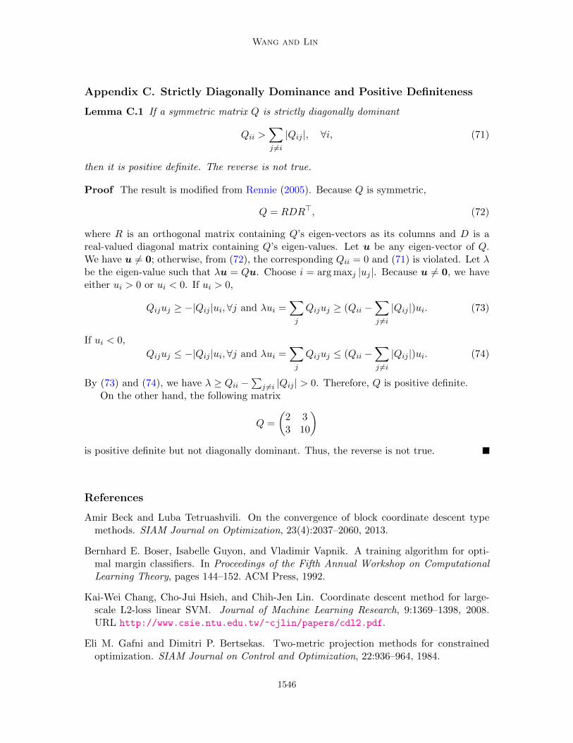
Q =
(2 33 10
)is positive definite but not diagonally dominant. Thus, the reverse is not true.
References
Amir Beck and Luba Tetruashvili. On the convergence of block coordinate descent typemethods. SIAM Journal on Optimization, 23(4):2037–2060, 2013.
Bernhard E. Boser, Isabelle Guyon, and Vladimir Vapnik. A training algorithm for opti-mal margin classifiers. In Proceedings of the Fifth Annual Workshop on ComputationalLearning Theory, pages 144–152. ACM Press, 1992.
Kai-Wei Chang, Cho-Jui Hsieh, and Chih-Jen Lin. Coordinate descent method for large-scale L2-loss linear SVM. Journal of Machine Learning Research, 9:1369–1398, 2008.URL http://www.csie.ntu.edu.tw/~cjlin/papers/cdl2.pdf.
Eli M. Gafni and Dimitri P. Bertsekas. Two-metric projection methods for constrainedoptimization. SIAM Journal on Control and Optimization, 22:936–964, 1984.
G. H. Golub and C. F. Van Loan. Matrix Computations. The Johns Hopkins UniversityPress, third edition, 1996.
Clifford Hildreth. A quadratic programming procedure. Naval Research Logistics Quarterly,4:79–85, 1957.
Jean-Baptiste Hiriart-Urruty and Claude Lemarechal. Fundamentals of convex analysis.Springer Verlag, 2001.
Chia-Hua Ho and Chih-Jen Lin. Large-scale linear support vector regression. Journal ofMachine Learning Research, 13:3323–3348, 2012. URL http://www.csie.ntu.edu.tw/
~cjlin/papers/linear-svr.pdf.
Alan J Hoffman. On approximate solutions of systems of linear inequalities. Journal ofResearch of the National Bureau of Standards, 49(4):263–265, 1952.
Cho-Jui Hsieh, Kai-Wei Chang, Chih-Jen Lin, S. Sathiya Keerthi, and Sellamanickam Sun-dararajan. A dual coordinate descent method for large-scale linear SVM. In Proceedingsof the Twenty Fifth International Conference on Machine Learning (ICML), 2008. URLhttp://www.csie.ntu.edu.tw/~cjlin/papers/cddual.pdf.
Wu Li. Sharp Lipschitz constants for basic optimal solutions and basic feasible solutions oflinear programs. SIAM Journal on Control and Optimization, 32(1):140–153, 1994.
Chih-Jen Lin, Ruby C. Weng, and S. Sathiya Keerthi. Trust region Newton method forlarge-scale logistic regression. Journal of Machine Learning Research, 9:627–650, 2008.URL http://www.csie.ntu.edu.tw/~cjlin/papers/logistic.pdf.
Zhi-Quan Luo and Paul Tseng. On the convergence of coordinate descent method forconvex differentiable minimization. Journal of Optimization Theory and Applications, 72(1):7–35, 1992a.
Zhi-Quan Luo and Paul Tseng. On the linear convergence of descent methods for convexessentially smooth minimization. SIAM Journal on Control and Optimization, 30(2):408–425, 1992b.
Zhi-Quan Luo and Paul Tseng. Error bounds and convergence analysis of feasible descentmethods: a general approach. Annals of Operations Research, 46:157–178, 1993.
Olvi L. Mangasarian and Tzong-Huei Shiau. Lipschitz continuity of solutions of linearinequalities, programs and complementarity problems. SIAM Journal on Control andOptimization, 25(3):583–595, 1987.
Yurii E. Nesterov. Efficiency of coordinate descent methods on huge-scale optimizationproblems. SIAM Journal on Optimization, 22(2):341–362, 2012.
Jong-Shi Pang. A posteriori error bounds for the linearly-constrained variational inequalityproblem. Mathematics of Operations Research, 12(3):474–484, 1987.
John C. Platt. Fast training of support vector machines using sequential minimal opti-mization. In Bernhard Scholkopf, Christopher J. C. Burges, and Alexander J. Smola,editors, Advances in Kernel Methods - Support Vector Learning, Cambridge, MA, 1998.MIT Press.
Jason D. M. Rennie. Regularized logistic regression is strictly convex. Technical report,MIT, 2005. URL http://qwone.com/~jason/writing/convexLR.pdf.
Peter Richtarik and Martin Takac. Iteration complexity of randomized block-coordinatedescent methods for minimizing a composite function. Mathematical Programming, 144:1–38, 2014.
Ankan Saha and Ambuj Tewari. On the nonasymptotic convergence of cyclic coordinatedescent methods. SIAM Journal on Optimization, 23(1):576–601, 2013.
Ludwig Seidel. Ueber ein verfahren, die gleichungen, auf welche die methode der klein-sten quadrate fuhrt, sowie lineare gleichungen uberhaupt, durch successive annaherungaufzulosen. Abhandlungen der Bayerischen Akademie der Wissenschaften. Mathematisch-Naturwissenschaftliche Abteilung, 11(3):81–108, 1874.
Shai Shalev-Shwartz and Ambuj Tewari. Stochastic methods for l1 regularized loss mini-mization. In Proceedings of the Twenty Sixth International Conference on Machine Learn-ing (ICML), 2009.
Shai Shalev-Shwartz and Tong Zhang. Stochastic dual coordinate ascent methods for reg-ularized loss minimization. Journal of Machine Learning Research, 14:567–599, 2013a.
Shai Shalev-Shwartz and Tong Zhang. Accelerated proximal stochastic dual coordinateascent for regularized loss minimization, 2013b. arXiv preprint arXiv:1309.2375.
Rachael Tappenden, Peter Richtarik, and Jacek Gondzio. Inexact coordinate descent: com-plexity and preconditioning, 2013. arXiv preprint arXiv:1304.5530.
Paul Tseng and Sangwoon Yun. Block-coordinate gradient descent method for linearlyconstrained nonsmooth separable optimization. Journal of Optimization Theory andApplications, 140:513–535, 2009.
Vladimir Vapnik. The Nature of Statistical Learning Theory. Springer-Verlag, New York,NY, 1995.
Jean-Philippe Vial. Strong and weak convexity of sets and functions. Mathematics ofOperations Research, 8(2):231–259, 1983.
Stephen J Wright. Accelerated block-coordinate relaxation for regularized optimization.SIAM Journal on Optimization, 22(1):159–186, 2012.