Iterative and Adaptive Processing for Multiuser Communication Systems Lance Linton B.Eng., M.Eng. College of Engineering and Science, Victoria University Submitted in fulfillment of the requirements of the degree of Doctor of Philosophy 15th April 2016
Transcript
Iterative and Adaptive Processing forMultiuser Communication Systems
Lance Linton B.Eng., M.Eng.
College of Engineering and Science,Victoria University
Submitted in fulfillment of the requirements of the degree of
Doctor of Philosophy
15th April 2016
ii
Abstract
The huge demand of wireless communications has driven the require-
ment for highly-efficient multiple-access communications schemes that
can accommodate multiple simultaneous users, yet provide performance
similar to single-user systems. Recently, iterative multiuser detection
schemes have shown to provide this high level of performance at a
manageable level of complexity. This thesis is concerned with iterative
detection of two non-orthogonal asynchronous access schemes: code-
division multiple-access (CDMA); and interleave-division multiple-access
(IDMA).
A multi-rate IDMA system is developed where different users transmit
data at different rates. High-rate users support multiple sub-streams,
each coded as an IDMA layer. The iterative receiver treats each IDMA
layer as a virtual user. Variance transfer analysis is employed to analyse
the receiver performance, which is then optimised by developing a power
allocation strategy. Simulation results demonstrate that the performance
of this proposed system is close to the theoretical limit in a Rayleigh
flat-fading environment.
Next, receiver performance is optimised by forward error correction
code allocation. For multiuser systems with dynamic loads, new users are
allocated codes according to the existing system load in order to optimise
receiver convergence. Small multiuser systems have performances that
approach the theoretical single-user bound.
The Golden Code is a “perfect” space-time block-code for 2× 2
multiple-antenna (MIMO) systems. It can simultaneously achieve both
full-diversity and -rate. A MIMO-IDMA multiuser detector is developed
to extend the golden code scheme to the multiuser case. Decoding is
performed by an iterative receiver whose complexity is linear in the
iii
number of users. In a Rayleigh flat-fading environment, simulation
results show that the proposed scheme can outperform other common
MIMO schemes and approaches within 0.25dB of the single-user bound.
The application of iterative multiuser detection to underwater acous-
tic communications is considered next. Designing reliable communication
systems for the underwater acoustic channel has proven to be very chal-
lenging. A major channel impairment is the multipath interference
caused by multiple reflections of the acoustic signal from the water
surface and bottom. These reflections occur at small grazing angles and
with small reflection losses, causing both long delay spread and large
multipath amplitudes in the received signal.
The large delay-spread implies that single-carrier communication will
be plagued by inter-symbol interference (ISI) that spans many symbols.
As an alternative, multi-carrier modulation (MCM) has been proposed
to increase the symbol interval and thereby decrease the ISI span. We
combine Orthogonal Frequency-Division Multiplexing (OFDM), a low-
complexity spectrally-efficient MCM technique, with an IDMA overlay
to develop a multiple-access communications system that provides robust
performance in the presence of large time-delay spread and the other
impairments presented by the shallow water acoustic channel.
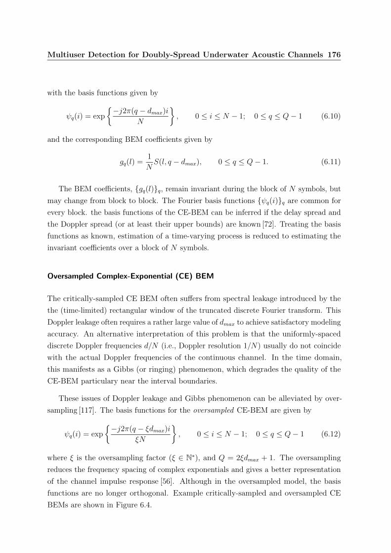
Finally, we consider multiuser communications in doubly-spread
underwater acoustic channels, where the relative motion between the
transmitter, receiver, and scattering objects imparts each path with a
unique Doppler shift. In this case, the orthogonality of OFDM is lost,
leading to subcarrier interference which greatly complicates optimal
data detection. Therefore, single-carrier system is considered with a
non-linear Kalman filter as equalizer. The doubly-selective channel is
modelled using basis expansion models (BEMs), a low-rank channel
model that exploits the inherent structure in the channel response. The
use of basis functions can turn a time-varying system identification
problem into a time-invariant one, thereby reducing the number of
parameters to estimate. The receiver uses a semi-blind iterative channel
estimation algorithm to estimate the channel parameters. Experimental
results demonstrate robust performance in underwater channels with
simultaneously large delay- and Doppler-spreads.
iv
Declaration
I, Lance Linton, declare that this PhD thesis entitled “Iterative and
Adaptive Processing for Multiuser Communication Systems” is no more than
100,000 words in length including quotes and exclusive of tables, figures,
appendices, bibliography, references and footnotes. This thesis contains no
material that has been submitted previously, in whole or in part, for the award
of any other academic degree or diploma. Except where otherwise indicated,
this thesis is my own work.
Lance Linton
15th April 2016
v
Acknowledgements
Of the many people who deserve thanks, some are particularly prominent, such as my
supervisors, Prof. Michael Faulker, Assoc. Prof. Patrick Leung, and Dr. Phillip Conder.
Their invaluable advice, guidance, and encouragement have made all of this possible.
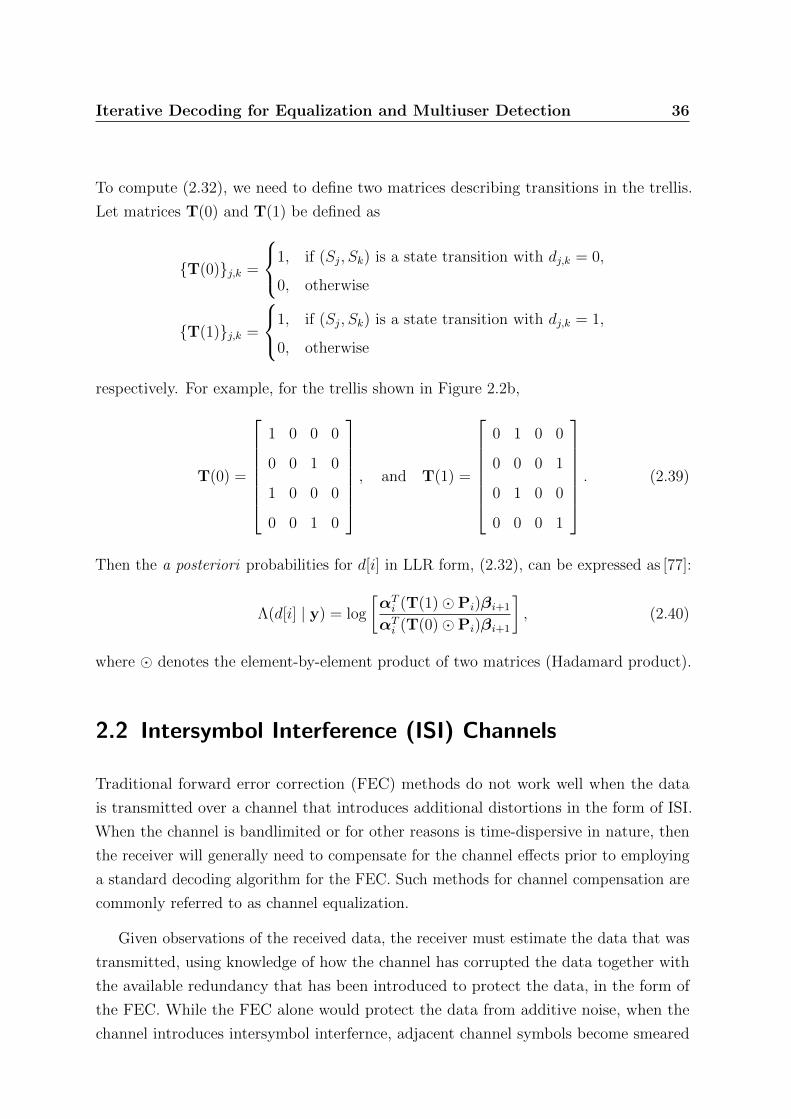
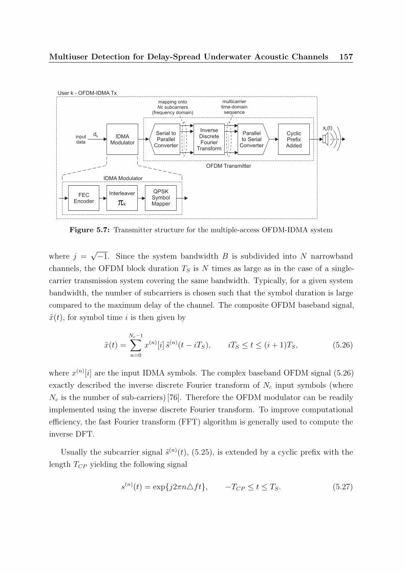
where ⊕ represents modulo-2 addition. The equations in (2.1) can be more concisely
represented by the generator polynomial (1 +D2, 1 +D +D2), where D is equivalent to
the discrete-time delay operator z−1.
Generally, convolutional coding schemes are designed so that the encoder starts from
a known initial state, and ends at a known termination state. For the example encoder
of Figure 2.1b, we assume that the two delay elements in the circuit are zero at the
beginning of the encoding process (time i = 0) and at the end (time i = M − 1). To
achieve the latter assumption, the last two input data bits, d[M − 2] and d[M − 1],
Iterative Decoding for Equalization and Multiuser Detection 26
must be zero, which implies a small rate loss. This loss can be controlled by using long
sequences (i.e., large values of M), or can be avoided by using tail-biting encoding [136]
[48].
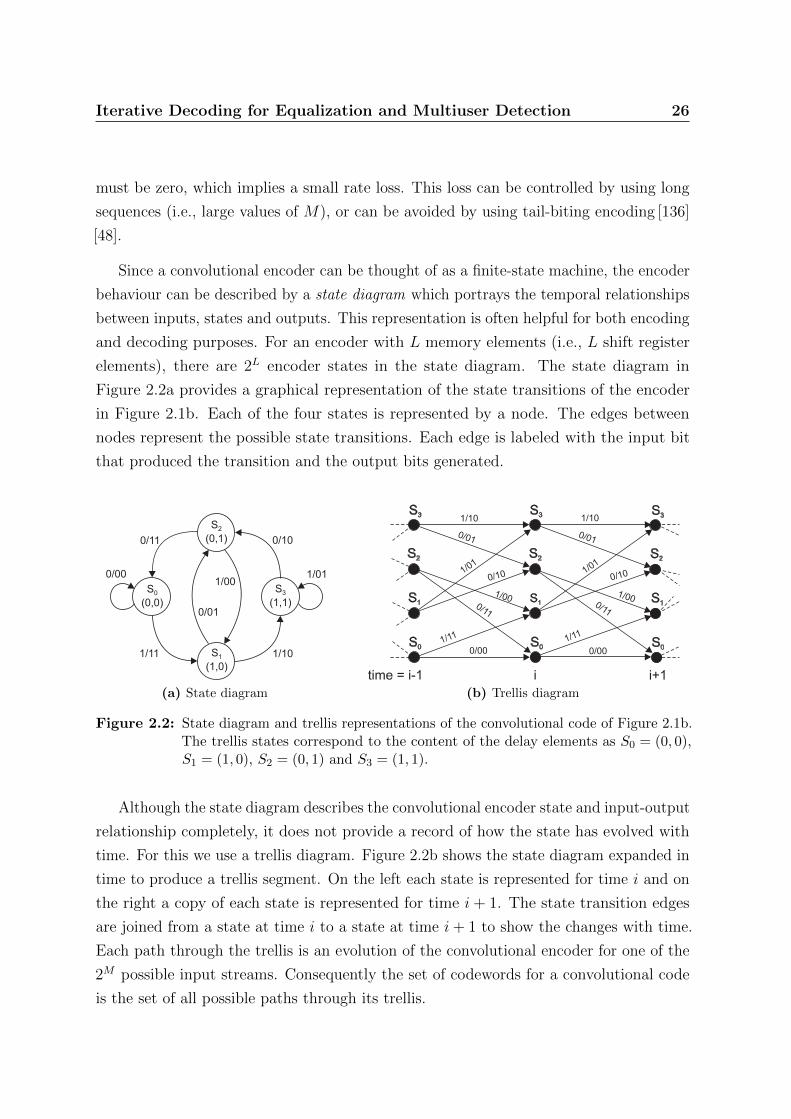
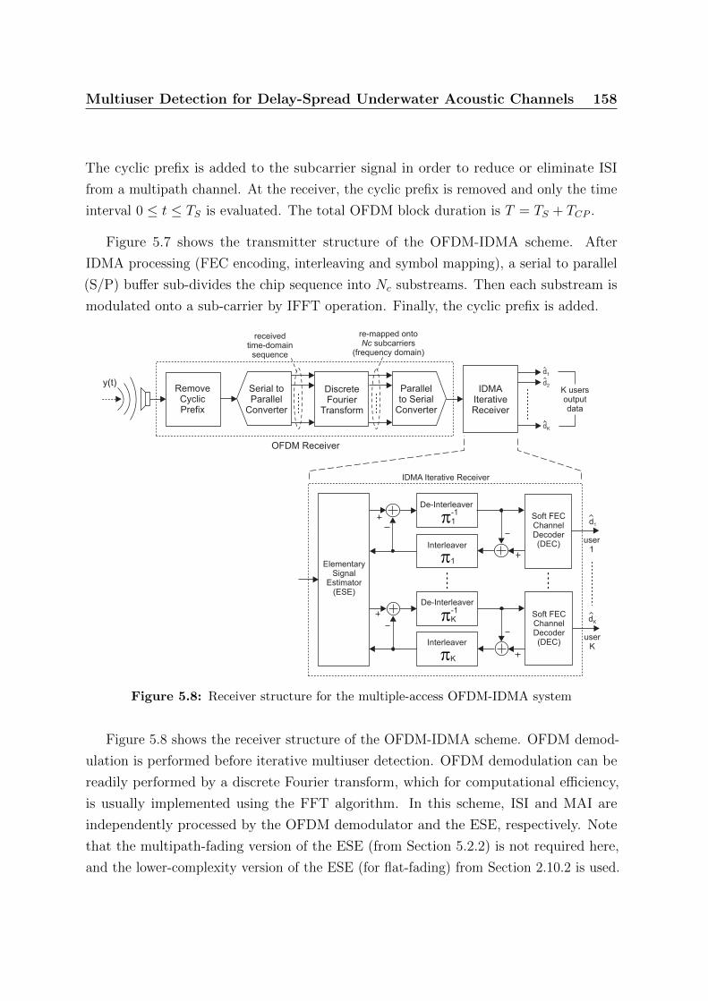
Since a convolutional encoder can be thought of as a finite-state machine, the encoder
behaviour can be described by a state diagram which portrays the temporal relationships
between inputs, states and outputs. This representation is often helpful for both encoding
and decoding purposes. For an encoder with L memory elements (i.e., L shift register
elements), there are 2L encoder states in the state diagram. The state diagram in
Figure 2.2a provides a graphical representation of the state transitions of the encoder
in Figure 2.1b. Each of the four states is represented by a node. The edges between
nodes represent the possible state transitions. Each edge is labeled with the input bit
that produced the transition and the output bits generated.
0/00 1/01
0/11
1/11 1/10
0/10
1/00
0/01
S
(0,0)0 S
(1,1)3
S
(1,0)1
S
(0,1)2
(a) State diagram
S3
S2
S1
S0
time = i-1
S3
S2
S1
S0
S3
S2
S1
S0
1/10
0/00
0/10
1/00
1/11
0/11
1/01
0/01
1/10
0/00
0/10
1/00
1/11
0/11
1/01
0/01
i i+1
(b) Trellis diagram
Figure 2.2: State diagram and trellis representations of the convolutional code of Figure 2.1b.The trellis states correspond to the content of the delay elements as S0 = (0, 0),S1 = (1, 0), S2 = (0, 1) and S3 = (1, 1).
Although the state diagram describes the convolutional encoder state and input-output
relationship completely, it does not provide a record of how the state has evolved with
time. For this we use a trellis diagram. Figure 2.2b shows the state diagram expanded in
time to produce a trellis segment. On the left each state is represented for time i and on
the right a copy of each state is represented for time i+ 1. The state transition edges
are joined from a state at time i to a state at time i+ 1 to show the changes with time.
Each path through the trellis is an evolution of the convolutional encoder for one of the
2M possible input streams. Consequently the set of codewords for a convolutional code
is the set of all possible paths through its trellis.
Iterative Decoding for Equalization and Multiuser Detection 27
This trellis representation enables optimal decoding of convolutional codes with
reasonable complexity. Each path in the trellis corresponds to a codeword, and so the
maximum likelihood (ML) decoder (which finds the most likely codeword) searches for
the most likely path in the trellis. Alternatively, each edge in the trellis can correspond
to a particular input: the bit-wise maximum a posteriori (MAP) decoder, which searches
for the maximum-probability input bit, calculates the probability of each trellis edge [48].
2.1.2 System Model
Conv.Encoder
SP
PS
MAPDecoder
SymbolMapperd[i] d[i]
Transmitter Receiver
AGWN
n[i]
BI-AWGN Channel
h0
ChannelCoefficient
(1)c [i]
(n)c [i]
y [i](1)
y [i](n)
x[i] y[i]c[i]
0-1+1
1
Figure 2.3: System model for a coded transmission over a memoryless AWGN channel
Figure 2.3 shows the system model for a convolutional-coded transmission scheme.
The input data sequence d = [ d[0], d[1], . . . , d[M − 1] ]T is encoded by the convolutional
encoder (with rate Rc) generating a n-bit coded vector, c[i], for each data bit, d[i], i.e.,
c =[cT [0], cT [1], . . . , cT [M − 1]
]Twhere c[i] =
[c(1)[i], . . . , c(n)[i]
]T(2.2)
The parallel-to-serial converter (P/S) concatenates M of the c[i] vectors to form a N -bit
frame. Hence, (2.2) can be restated as c = [ c[0], c[1], . . . , c[N − 1] ]T , where N is the
frame length (N = nM), and the elements of c are referred to as coded bits. The coded
bit sequence c is then BPSK modulated, producing the symbol sequence x, which is
This trellis description can be used to efficiently compute the APPs, P (x[i] | y).
+1/+1.63 -1/-1.63
+1/+0.815
-1/+0.815 -1/-0.815
+1/-0.815
-1/0
+1/0
S0
S3
S1
S2
(+1,-1)
(+1,+1)
(-1,+1)
(-1,-1)
(a) State diagram
S3
S2
S1
S0
time = i-1
S3
S2
S1
S0
S3
S2
S1
S0
-1/-1.63
+1/+1.63
+1/0
-1/0
-1/+0.815
+1/+0.815
-1/-0
.815
+1/-0.815
-1/-1.63
+1/+1.63
+1/0
-1/0
-1/+0.815
+1/+0.815
-1/-0
.815
+1/-0.815
i i+1
(b) Trellis diagram
Figure 2.7: State diagram and trellis representations of the channel in Figure 2.5. The statesS0 = (+1,+1), S1 = (−1,+1), S2 = (+1,−1), S3 = (−1,−1) are the possiblecontents of the channel model delay elements.
The approach of separating the equalization and decoding tasks assumes that the
transmitted symbols, x[i], are i.d.d. random variables, ie
P (x) =N−1∏i=0
P (x[i]) (2.52)
and x[i] takes on values +1 and −1 equally for all i. With this assumption, the BCJR
algorithm (of Section 2.1.4) can be adapted to efficiently compute P (x[i] | y).
The probability that the transmitted sequence path in the trellis contained the branch
(Sr, Ss, xr,s, vr,s) at time i, i.e., P (ψi = Sr, ψi+1 = Ss | y) can be computed by the BCJR
algorithm[6], [97] based on the decomposition of the joint distribution p(ψi, ψi+1,y) given
by
p(ψi, ψi+1,y) = P (ψi, ψi+1 | y)p(y). (2.53)
The received signal sequence y in p(ψi, ψi+1,y) can be written as
Iterative Decoding for Equalization and Multiuser Detection 47
Note that (2.57) includes the demapping operation x[i]→ b[i], where
Λ(b[i] | y) = logP (b[i] = 0 | y)
P (b[i] = 1 | y)= log
P (x[i] = +1 | y)
P (x[i] = −1 | y)
Finally, the code bit estimates b[i] are computed from the sign of Λ(b[i] | y) as in (2.50).
The BCJR algorithm for MAP equalization can be concisely described in terms of
matrix operations. For a trellis with a set of states S, denote the following vectors and
matrices:
• αi as the set of |S|× 1 vectors of the forward probabilities (αi(ψ) values), as defined
in (2.34);
• βi as the set of |S|× 1 vectors of backward probabilities (βi(ψ) values), as defined
in (2.35);
• Pi as the set of |S|× |S| probability matrices as defined in (2.36); and
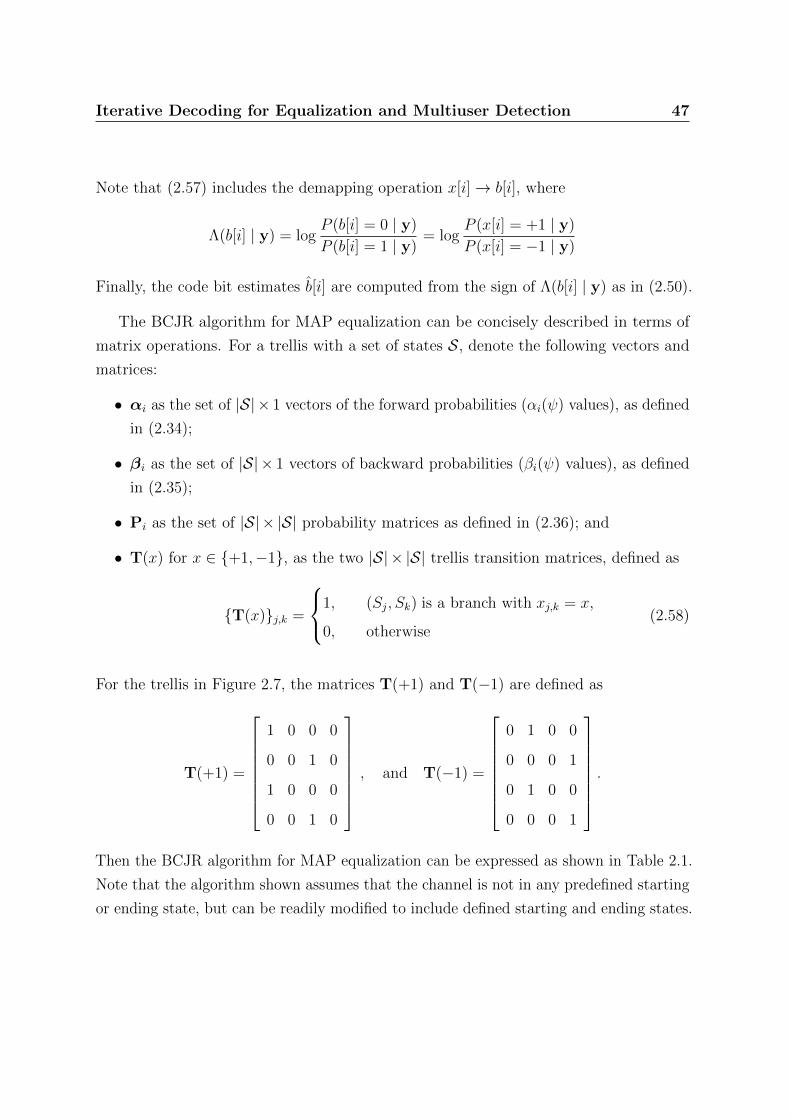
• T(x) for x ∈ +1,−1, as the two |S|× |S| trellis transition matrices, defined as
T(x)j,k =
1, (Sj, Sk) is a branch with xj,k = x,
0, otherwise(2.58)
For the trellis in Figure 2.7, the matrices T(+1) and T(−1) are defined as
T(+1) =
1 0 0 0
0 0 1 0
1 0 0 0
0 0 1 0
, and T(−1) =
0 1 0 0
0 0 0 1
0 1 0 0
0 0 0 1
.
Then the BCJR algorithm for MAP equalization can be expressed as shown in Table 2.1.
Note that the algorithm shown assumes that the channel is not in any predefined starting
or ending state, but can be readily modified to include defined starting and ending states.
Iterative Decoding for Equalization and Multiuser Detection 48
1. Initialization: calculate matrices Pi for i = 0, 1, . . . , N − 1, where
Pir,s = γi(Sr, Ss) and
γi(Sr, Ss) =
P (x[i] = xr,s)p(y[i] | v[i] = vr,s), (Sr, Ss) ∈ T
0, (Sr, Ss) /∈ T .
2. Forward recursion: calculate vectors αi for i = 0, 1, . . . , N − 1, where
α0 = [ 1, 1, . . . , 1 ]T and
αi = PTi−1αi−1, i = 1, 2, . . . , N − 1.
3. Backward recursion: calculate vectors βi for i = N,N − 1, . . . , 0, where
βN = [ 1, 1, . . . , 1 ]T and
βi = Piβi+1, i = N − 1, N − 2, . . . , 1.
4. Output: calculate code bit APPs in LLR form, Λ(b[i] | y), using
Λ(b[i] | y) = log
[αTi (T(+1)Pi)βi+1
αTi (T(−1)Pi)βi+1
], i = 0, 1, . . . , N − 1.
Table 2.1: MAP equalization using the BCJR algorithm
In a practical implementation of the algorithm, a frequent re-normalization of the
vectors is necessary to avoid numerical underflow. That is, after each step in the recursion
to compute αi and βi, both vectors are normalized using (2.33).
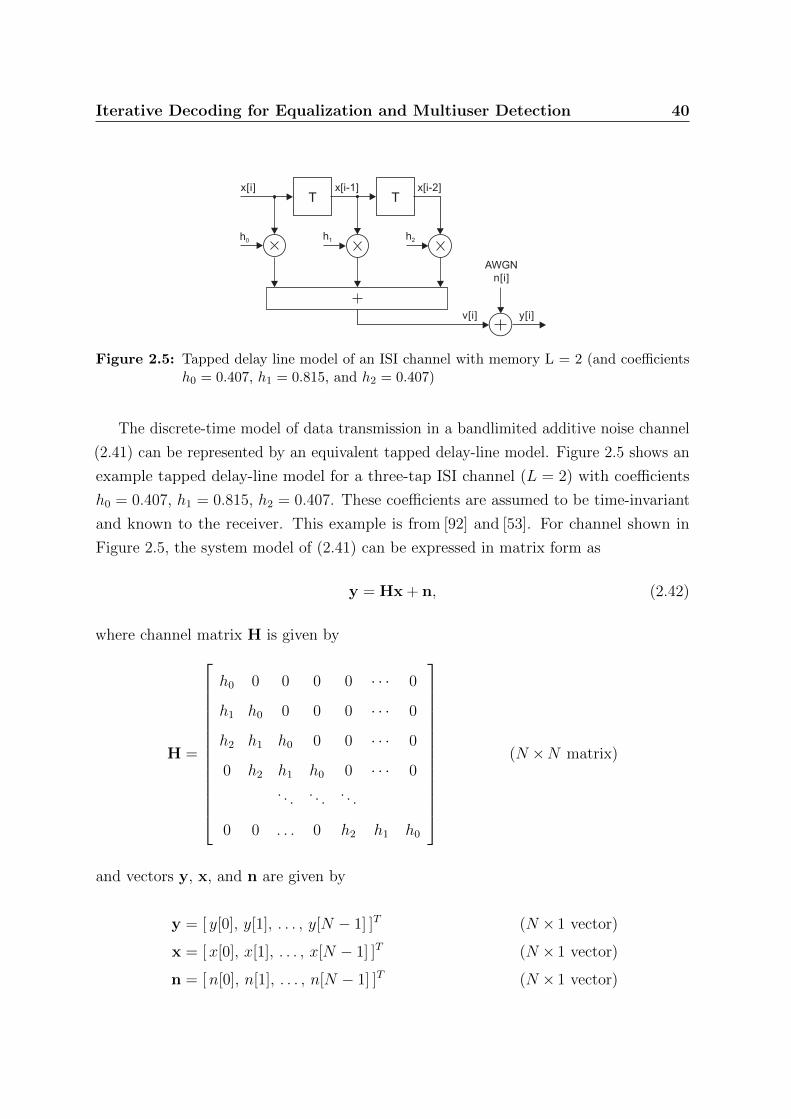
2.3.2 Linear Equalization and Symbol Detection
The computational complexity of the trellis-based approaches is determined by the
number of trellis states, equal to 2QL, where Q is the number of bits mapped onto each
symbol and L is the number of delay elements in the tapped delay line channel model
(Figure 2.5). Therefore, the computational complexity of trellis-based equalization can
become prohibitive for large signal constellations or long channel-delay spreads.
Iterative Decoding for Equalization and Multiuser Detection 49
In contrast to trellis-based equalization, linear-filter-based approaches perform only
simple operations on the received symbols, which are applied sequentially to a subset
of the observed symbols. Consider the transmitted symbols in the interval x[i −δ], . . . , x[i], . . . , x[i+ δ], where, for example, δ = 6. This subset of transmitted symbols,
Iterative Decoding for Equalization and Multiuser Detection 52
Substituting (2.73) into (2.69) and (2.69), the MMSE linear equalizer (for the case where
there is no a priori information about the symbols available) is given by [112] [92]
x[i] = wTi yi, where wi =
(σ2I∆ + HH
T)−1
He. (2.74)
The estimates x[i] are usually not in the symbol alphabet +1, 1 and the decision
whether x[i] = +1 or x[i] = −1 is usually based on the estimation error ε[i] = x[i]− x[i].
Given the estimator (2.62)-(2.63), the p.d.f. of the estimation error, p(ε[i]), can be
assumed to be Gaussian and is given by [41]
p(ε[i]) =1√
2πVarε[i]exp
ε2[i]
2Varε[i]
,
where the mean and variance are given by
Eε[i] = 0, and Varε[i] = Varx[i] −wTi He,
respectively. The hard decision of x[i] is the symbol x ∈ +1,−1 that maximizes p(ε[i]),
which is the symbol x of closest distance to x[i], i.e.,
x[i] = arg minx∈+1,−1
|x− x[i] |.
2.3.3 Trellis-Based MAP FEC Decoding
The symbol a posteriori probabilities in LLR form, Λ(x[i] | y) ), output from the
equalizer/detector are demapped and deinterleaved to form the code bit probabilities,
Λ(c[i] | y), input to the FEC decoder. In LLR form, the code bit probabilities Λ(c[i] | y)
can be converted back to probability form using
P (c[i] = 1 | y) =1
2
1− tanh
(Λ(c[i] | y)
2
)(2.75)
and
P (c[i] = 0 | y) =1
2
1 + tanh
(Λ(c[i] | y)
2
). (2.76)
Iterative Decoding for Equalization and Multiuser Detection 53
The set of probabilities input to the FEC decoder is denoted p, where
p = [P (c[0] | y), P (c[1] | y), . . . , P (c[N − 2] | y), P (c[N − 1] | y) ]T (2.77)
Using these input probabilities, the decoder is tasked with decoding the FEC code,
which in this case, is a binary convolutional code. The BCJR algorithm operating on a
trellis description for the code can used here as an efficient MAP decoder for computing
estimates of the transmitted data bits, d[i]. In Section 2.1.4, the BCJR algorithm was
used as a MAP decoder for convolutional codes, but for case where channel observations
are used as input. In this section, the BCJR algorithm is modified for the case where
code bit probabilities are used as input.
Consider the convolutional encoder of Figure 2.1b and the corresponding trellis descrip-
tion of Figure 2.2b. The trellis branches are denoted by the tuple (Sr, Ss, dr,s, c(1)r,s , c
(2)r,s ),
where dr,s is the input bit d[i] and (c(1)r,s , c
(2)r,s ) are the two output bits (c(1)[i], c(2)[i])
belonging to the state transition (ψi = Sr, ψi+1 = Ss). The set T of valid transitions is
listed in (2.15).
The MAP decoder processes the N -bit block of coded bit probabilities in M state
transitions. Therefore, for notational convenience, the set of coded bit probabilities in
(2.77) can be restated as
p =[P (c(1)[0] | y), P (c(2)[0] | y), . . . , P (c(1)[M − 1] | y), P (c(2)[M − 1] | y)
]T(2.78)
where there are two coded bits per state transition since the FEC encoder uses a rate-1/2
code, i.e., N = 2M for Rc = 1/2. The change in notation from (2.77) to (2.78) represents
the serial-to-parallel conversion process at the input of the MAP decoder (as shown, for
example, in Figure 2.3).
To apply the BCJR MAP algorithm from Section 2.1.4, the computation of the
transition probabilities, γi(ψi, ψi+1), must be modified to use code bit probabilities as
input (instead of channel observations). For probabilistic input, γi(ψi, ψi+1) is computed
as
γi(Sr, Ss) =
P (d[i] = dr,s)P (c(1)[i] = c(1)r,s | y)P (c(2)[i] = c
(2)r,s | y), (Sr, Ss) ∈ T
0, (Sr, Ss) /∈ T(2.79)
Iterative Decoding for Equalization and Multiuser Detection 54
where P (d[i] = 0) = P (d[i] = 1) = 1/2 from the assumption that the data bits, d[i], are
i.i.d. The code bit probabilities are computed from (2.75) and (2.76).
The matrices T(x) for x ∈ 0, 1 are defined as
T(x)j,k =
1, (Sj, Sk) is a branch with dj,k = x,
0, otherwise.(2.80)
and the BCJR algorithm for MAP FEC decoding (with probabilistic input) can be
expressed as shown in Table 2.2. Note that the initialization of the αi and βi vectors
assumes that the encoder starts from state S0 at time i = 0 and terminates at state S0
at time i = M − 1.
When the soft FEC decoder is used in turbo equalization or turbo multiuser-detection
configurations (described in later sections), the decoder is required to compute the
code bit APPs, Λ(c[i] | p), in addition to the data bit APPs, Λ(d[i] | p). In turbo
configurations, the code bit APPs, Λ(c[i] | p), serve as a priori information for the
equalizer or multiuser detector algorithm. Code bit APPs can be computed using the
BCJR algorithm in Table 2.2 by changing the definitions of the T(x) matrices. For APPs
Λ(c(1)[i] | p), i = 0, 1, . . . ,M − 1 (in LLR from), matrices T(x) for x ∈ 0, 1 are defined
as
T(x)j,k =
1, (Sj, Sk) is a branch with c(1)j,k = x,
0, otherwise.(2.81)
Similarly, for APPs Λ(c(2)[i] | p), i = 0, 1, . . . ,M − 1 (in LLR form), matrices T(x) for
x ∈ 0, 1 are defined as
T(x)j,k =
1, (Sj, Sk) is a branch with c(2)j,k = x,
0, otherwise.(2.82)
Iterative Decoding for Equalization and Multiuser Detection 55
1. Initialization: calculate matrices Pi for i = 0, 1, . . . ,M − 1, where
Pir,s = γi(Sr, Ss) and
γi(Sr, Ss) =
P (d[i] = dr,s)P (c(1)[i] = c(1)r,s | y)P (c(2)[i] = c
(2)r,s | y), (Sr, Ss) ∈ T
0, (Sr, Ss) /∈ T
2. Forward recursion: calculate vectors αi for i = 0, 1, . . . ,M − 1, where
α0 = [ 1, 0, . . . , 0 ]T and
αi = PTi−1αi−1, i = 1, 2, . . . ,M − 1.
3. Backward recursion: calculate vectors βi for i = M,M − 1, . . . , 1, where
βM = [ 1, 0, . . . , 0 ]T and
βi = Piβi+1, i = M − 1,M − 2, . . . , 1.
4. Output: calculate data bit APPs in LLR form, Λ(d[i] | p), using
Λ(d[i] | p) = log
[αTi (T(0)Pi)βi+1
αTi (T(1)Pi)βi+1
], i = 0, 1, . . . ,M − 1.
where T(x) is defined in (2.80). Λ(c(1)[i] | p) and Λ(c(2)[i] | p) are
computed similarly, using T(x) defined in (2.81) and (2.82), respectively.
Table 2.2: MAP FEC decoding using the BCJR algorithm
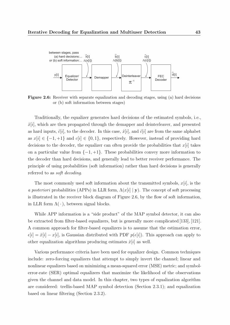
2.3.4 System Performance
The performance of the separate equalization and decoding schemes is evaluated for the
ISI channel model of Figure 2.5. The schemes use an input data block length (M) of
512 bits with forward error correction performed by the rate-1/2 convolutional encoder
of Figure 2.1b, resulting in a coded block length (N) of 1024 bits. The coded bits are
scrambled using a random interleaver and mapped onto BPSK symbols. Figure 2.9
compares the receiver performance using the MAP symbol detector (‘MAP/APP Det.’)
of Section 2.3.1 and the MMSE linear equalizer (‘LMMSE Eq.’) of Section 2.3.2. In both
Iterative Decoding for Equalization and Multiuser Detection 56
cases, FEC decoding is performed using the BCJR algorithm of Section 2.3.3. The effect
of passing hard bit estimates and soft information from the equalizer to the decoder is
also compared.
It can be seen that MAP symbol detection (using the BCJR algorithm) provides
superior performance compared to the MMSE linear equalizer, but at the cost of additional
computational complexity. Note also that passing soft information between the equalizer
and decoder provides a 2dB gain in SNR compared to passing hard bit decisions.
SNR(dB)
Da
ta B
it E
rro
r R
ate
0 4 8 102 6
10-5
10-3
10-2
10-1
100
10-4
Separate Equalization and Decoding (Non-Iterative)
LMMSE Eq. (Hard)
LMMSE Eq. (Soft)
MAP/APP Det. (Hard)
MAP/APP Det. (Soft)
Figure 2.9: System performance of separate equalization and decoding schemes. Performanceof equalizer types (MAP symbol detection, and linear MMSE equalization) iscompared. System performance when passing hard estimates, and soft information,from the equalizer to the decoder is also compared.
The performance of these separate equalization and decoding schemes is suboptimal
because of assumptions of independence in the derivation of the soft information ex-
changed. In particular, the computation of the APPs P (x[i] | y) assumes that all 2N
possible sequences x[i]N−1i=0 are equally likely, i.e., P (x) = 1/2N (from the assumption
that symbols, x[i], are i.d.d). However, there are only 2M valid sequences of x[i]N−1i=0 ,
each belonging to a particular input data sequence d[i]M−1i=0 . Therefore, the equalizer
Iterative Decoding for Equalization and Multiuser Detection 57
performance would be significantly improved if the APPs were computed as
P (x[i] = x | y) =∑
all 2M valid x:x[i]=x
p(y | x)P (x)
p(y), (2.83)
where P (x) = 1/2M for valid x. However, this approach would require exhaustive search
methods, since trellis-based methods (such as the BCJR algorithm) could no longer be
used, and the resulting computational complexity would be prohibitive.
2.4 Turbo Equalization for ISI Channels
The MAP symbol detector computes symbol estimates using the MAP rule
x[i] = arg maxx∈+1,−1
P (x[i] = x | y), i = 0, 1, . . . , N − 1, (2.84)
where, using Bayes’ rule, the a posteriori probabilities can be computed from
P (x[i] = x | y) =∑
x:x[i]=x
p(y | x)P (x), x ∈ +1,−1. (2.85)
Here p(y | x) is the likelihood function and P (x) is the a priori probability. Note that
the marginal probability, p(y), does not have to be included in this form of the equation.
Hence, MAP detection can be thought of as a process that takes a series of observations,
y, and bit-wise a priori probabilities, P (x[i])i, and computes bit-wise a posteriori
probabilities, P (x[i] | y)i, as shown in the block diagram model in Figure 2.10.
MAP Detector
a posterioriprobabilities
a prioriprobabilities
observations
y
P( | )x y
P( )x
LikelihoodCalculation
PosteriorCalculation
P( | )y x
Figure 2.10: The MAP detection process in block diagram form, which takes a priori prob-abilities and observations as input and produces a posteriori probabilities asoutput
Iterative Decoding for Equalization and Multiuser Detection 58
In the BCJR equalization algorithm of Section 2.3.1, the a posteriori probabilities
are formed from the transition probabilities, γi(Sr, Ss), computed from (2.56), i.e.,
The interleaver and deinterleaver are incorporated into the iterative loop to further
disperse the direct feedback effect. In particular, the BCJR algorithm creates output
that is locally highly-correlated, but the use of an interleaver can largely suppress the
correlations between neighboring symbols.
The operation of the turbo equalization receiver is shown in Table 2.3. The notation:
Λ1(b | y) = MAP Equalizer(λ2(b | p))
represents the generation of APP LLRs, Λ1(b | y), by the MAP Equalizer from observa-
tions, y, and a priori LLRs, λ2(b | p), using the BCJR algorithm described in Table 2.1.
Iterative Decoding for Equalization and Multiuser Detection 61
Similarly, the notation:
Λ2(c | p) = MAP FEC Decoder(λ1(c | y))
represents the generation of APP LLRs, Λ1(b | y), by the MAP FEC Decoder from the
a priori LLRs, λ2(c | y), using the BCJR algorithm described in Table 2.2.
While the turbo equalization algorithm presented is based on two MAP algorithms,
any pair of equalization and FEC decoding algorithms that make use of soft information
can be used as constituent algorithms in the turbo equalizer.
For example, the linear MMSE equalizer in Section 2.3.2 can use a priori information
about the transmitted symbol x[i] to compute symbol statistics Ex[i] and Varx[i](using (2.71)-(2.72)) which are then incorporated into the MMSE filter, (2.69)-(2.70),
to compute symbol estimate, x[i], and APP LLR, Λ1(x[i] | y). As with the MAP
equalization algorithm, the APP LLR is computed the constraint that Λ1(x[i] | y) is not
a function of the a priori LLR, λ2(b[i] | p), at the same index i. This helps to avoid short
feedback cycles, and is equivalent to extracting only the extrinsic part of the information
in the iterative scheme [53]. Note also that there are several low-complexity alternatives
for re-estimating x[i], e.g. [53], [121], [122], [33], [120], [98], [139].
Figure 2.12 shows the performance of the turbo equalization scheme (of Figure 2.11
and Table 2.3) for the ISI channel model of Figure 2.5. The scheme is evaluated for an
input data block length (M) of 512 bits with forward error correction performed by the
rate-1/2 convolutional encoder of Figure 2.1b, resulting in a coded block length (N) of
1024 bits. The coded bits are scrambled using a random interleaver and mapped onto
BPSK symbols.
Figure 2.12a shows the effect of receiver iterations for a turbo equalizer using the
MAP symbol detector of Section 2.3.1, while Figure 2.12b shows the effect of receiver
iterations for a turbo equalizer using the MMSE linear equalizer of Section 2.3.2. In both
cases, FEC decoding is performed using the BCJR algorithm of Section 2.3.3. Note that
zero-iterations represents the first pass when there is no a-priori information available
for APP equalizer–this is equivalent to the separate equalization and decoding scheme
(with soft information) evaluated in Section 2.3.4. The ISI-free bound represents the
lower BER performance bound of the underlying rate-1/2 code used over an ISI-free
channel, i.e., the performance bound for the evaluated system.
Iterative Decoding for Equalization and Multiuser Detection 62
Turbo Equalization using MAP Symbol Detection
SNR (dB)
-2 0 2 4 6
Bit E
rro
r R
ate
10-5
10-3
10-2
10-1
100
10-4
ISI-Free Bound
0 Iterations
1 Iteration
2 Iterations
10 Iterations
(a) Performance of turbo equalization using MAP symbol detection
SNR (dB)
-2 0 2 4 6
Bit E
rror
Rate
10-5
10-3
10-2
10-1
100
10-4
Turbo Equalization using Linear MSSE Equalizer
ISI-Free Bound
0 Iterations
1 Iteration
2 Iterations
10 Iterations
(b) Performance of turbo equalization using linear MMSE equalization
Figure 2.12: Performance of turbo equalization after 0, 1, 2, and 10 iterations using: (a)MAP symbol detection; and (b) linear MMSE equalization.
Iterative Decoding for Equalization and Multiuser Detection 63
Both schemes show significant BER performance gain over the iterations, with
performance approaching the ISI-free bound after 10 iterations. It is observed that turbo
equalization using MAP symbol detection provides superior performance compared to
the MMSE linear equalizer based scheme, but at the cost of additional computational
complexity. However, it is noted that for larger block lengths, M , the performance of
linear MMSE equalizer approaches that of the MAP detector [53], [121].
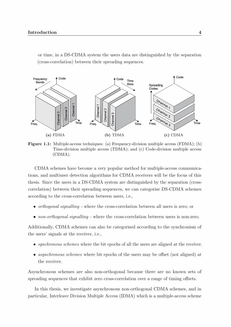
2.5 Code Division Multiple Access (CDMA) and
Multiuser Detection
For multiuser communications, CDMA is an attractive multiple-access technique that
has become widely used. Using the direct sequence spread-spectrum technique, each user
spreads its signal over the entire bandwith, such that when demodulating any particular
user’s data, the other users’ signals appear as pseudo white noise. A CDMA systems
are interference limited, meaning that multiple-access interference and intersymbol
interference (ISI) limit the system performance [127].
Multiuser detection (MUD) is the detection of data from multiple terminals in a
communication network when observed in a nonorthogonal multiplex, that is, when
derived from a nonorthogonal multiple-access channel. This situation may be the result
of system design, for example, in code-division multiple-access (CDMA) systems using
nonorthogonal spreading codes. It may also be the result of channel impairments in
orthogonally multiplexed systems, for example, in time-division multiple-access (TDMA)
wireless systems transmitting over multipath-fading delay-spread channels. Another
example is digital subscriber line (DSL) systems that are impaired by crosstalk and other
types of interference.
The fundamental concept of MUD is to make use of the known structure of all the
users’ transmitted signals, and the cross-correlations among these signals, in order to
improve the data detection process. Research has shown that the use of MUD can provide
significant performance advantages in interference-limited channels, and many advances
have been made in recent years [127], [134], [88], [102].
Optimal MUD techniques, based on maximum-likelihood (ML) or maximum a posteri-
ori probability (MAP) criteria, often achieve performance close to that of an interference-
free system. hat is free of interference. However, these methods have high computational
Iterative Decoding for Equalization and Multiuser Detection 64
complexity, particularly when compared with the processing resources available in most
communications receivers. As a result, considerably effort has been made to develop sub-
optimal low-complexity techniques that can achieve good performance. Linear multiuser
detection is a popular low-complexity technique that uses linear processing to suppress
interference, followed by simple quantization to perform data detection.
The computational complexity of optimal MUD techniques is further increased when
forward error correction (FEC) is considered in addition to nonorthogonal signaling.
In particular, the complexity of joint MUD and FEC decoding (based on ML or MAP
criteria) is prohibitively high. However, this combination can be considered as a serially
concatenated coding system, where the FEC code and multiple-access channel take the
roles of outer code and inner code, respectively [102]. This interpretation, provides the
basis for iterative MUD techniques to be developed using the turbo decoding concept
[12]. In these techniques, which are commonly known as turbo MUD [134], [88], the MUD
is used to provide tentative channel-symbol decisions to the FEC channel decoders, and
similarly, tentative channel-symbol decisions are produced by the channel decoders which
are fed back to the MUD. Several iterations between these two constituent processes
are made, with intermediate exchanges of soft channel symbol information. These turbo
MUD techniques have modest computational complexity, yet have been shown to provide
near-optimal performance.
2.5.1 Synchronous CDMA Signal Model
In CDMA systems, multiple users can share a common frequency band at the same time
by using different signature waveforms. Consider a CDMA channel that is shared by by
K simultaneous users. For simplicity, it is assumed that binary antipodal (BPSK) signals
are used to transmit the information from each user. The received signal, y(t), will
consist of the sum of antipodally modulated synchronous signature waveforms embedded
in additive white Gaussian noise:
y(t) =K∑k=1
Akbksk(t) + n(t), t ∈ [ 0, T ] (2.87)
where
• T is the symbol interval
• sk(t) is the deterministic signature waveform assigned to the k-th user.
Iterative Decoding for Equalization and Multiuser Detection 65
• Ak is the received amplitude of the k-th user’s signal. A2k is referred to as the energy
of the k-th user.
• bk is the bit transmitted by the k-th user, bk ∈ −1,+1
• n(t) is a zero-mean white Gaussian noise (AWGN) process with power spectral
density σ2. This models noise sources that are unrelated to the transmitted signal,
including thermal noise.
Each user is assigned a signature waveform sk(t) of duration T . A signature waveform
may be expressed as
sk(t) =L−1∑n=0
ak(n)pc(t− nTc), t ∈ [ 0, T ] (2.88)
where ak(n), 0 ≤ n ≤ L− 1 is a pseudo-noise (PN) code sequence consisting of L chips
that take values ± 1, pc(t) is a pulse of duration Tc, and Tc is the chip interval. Thus,
there are L chips per symbol and T = LTc. The signature waveforms are assumed to
be zero outside the interval [0, T ], and therefore, there is no intersymbol interference.
Additionally, it is also assumed that all K signature waveforms have unit energy, i.e.,
‖sk‖2 =
∫ T
0
s2k(t) dt = 1 (2.89)
The performance of various demodulation strategies depends on the signal-to-noise
ratios, Ak/σ, and on the similarity between the signature waveforms, quantified by their
cross-correlations, which for the synchronous case is defined as
ρij = ρij(0) =
∫ T
0
si(t)sj(t) dt. (2.90)
for the synchronous case.
2.5.2 Asynchronous CDMA Signal Model
In the synchronous model, bit epochs are aligned at the receiver. However, symbol-
synchronism is not necessary for CDMA to operate, and it is possible to let the users
transmit completely asynchronously. The asynchronous CDMA model is shown in
Figure 2.13 where time offsets are introduced to model the lack of alignment of the bit
epochs at the receiver: τk ∈ [0, T ), k = 1, . . . , K. The symbol epochs are defined with
Iterative Decoding for Equalization and Multiuser Detection 66
User 1
AWGN
s1(t)
y(t)S
b [i]1
s2(t)
b [i]2
s3(t)
b [i]3
n(t)
Delayt1
Delayt2
Delayt3
A1
A2
A3
User 2
User 3
x3(t)
x2(t)
x1(t)
Multiple Access Channel
(a) Asynchronous CDMA channel model for 3 users (K = 3)
T
User 2
User 1 ( =0)t1
User 3
b [0]1 b [1]1 b [2]1
b [0]2 b [1]2 b [2]2
b [0]3 b [1]3 b [2]3
2T 3T0 t2 t3 T+t2 T+t3time
(b) Asynchronism modelling using time offsets. Bit epochs for 3 users (K = 3)
Figure 2.13: Asynchronous CDMA channel model and asynchronism modelling using timeoffsets for 3 users (K = 3)
respect to an arbitrary origin (it is often advantageous to take τ1 = 0). Without loss of
generality, we assume that 0 ≤ τ1 ≤ τ2 ≤ · · · ≤ τK < T . Note that we still require the
symbol interval be identical for all users.
For the synchronous model it is sufficient to restrict attention to the received waveform
in an interval of length T , the bit duration. In the asynchronous case we must take into
account the fact that the users send a stream of bits. Without loss of generality, we
assume that all users transmit packets or frames of length N . Therefore the data block
for the k-th user is bk[i]N−1i=0 Generalising (2.87) to the asynchronous case, the CDMA
Iterative Decoding for Equalization and Multiuser Detection 67
channel model now becomes
y(t) =K∑k=1
Ak
N−1∑i=0
bk[i]sk(t− iT − τk) + σn(t), t ∈ [ 0, NT ], τk ∈ [ 0, T ) (2.91)
The synchronous channel corresponds to the special case of (2.91) where all the offsets
are identical, τk = 0 for 1 ≤ k ≤ K.
As with the synchronous channel, asynchronous channel performance depends on
the cross-correlation between the user signature waveforms. However for asynchronous
CDMA, the synchronous cross-correlation definition of (2.90) is not sufficient to determine
the performance, and two cross-correlations between every pair of signature waveforms
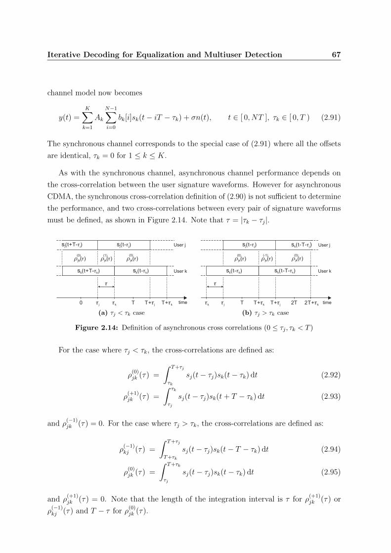
must be defined, as shown in Figure 2.14. Note that τ = |τk − τj|.
0 time
User j
User k
rjk( )t rjk( )t
t
sk(t-tk)sk(t+T-tk)
(0)
sj(t+T- )tj
tk T+tk
rjk( )t
sj(t-tj)
(1)
tj T T+tj
(0)
(a) τj < τk case
time
User k
User j
rjk( )t rjk( )t
t
sj(t-tj) sk(t-T-tj)
(0)
sk(t-T- )tk
tj T+tj
rjk( )t
sk(t-tk)
(-1)
tk T T+tk
(0)
2T+tk2T
(b) τj > τk case
Figure 2.14: Definition of asynchronous cross correlations (0 ≤ τj , τk < T )
For the case where τj < τk, the cross-correlations are defined as:
ρ(0)jk (τ) =
∫ T+τj
τk
sj(t− τj)sk(t− τk) dt (2.92)
ρ(+1)jk (τ) =
∫ τk
τj
sj(t− τj)sk(t+ T − τk) dt (2.93)
and ρ(−1)jk (τ) = 0. For the case where τj > τk, the cross-correlations are defined as:
ρ(−1)kj (τ) =
∫ T+τj
T+τk
sj(t− τj)sk(t− T − τk) dt (2.94)
ρ(0)jk (τ) =
∫ T+τk
τj
sj(t− τj)sk(t− τk) dt (2.95)
and ρ(+1)jk (τ) = 0. Note that the length of the integration interval is τ for ρ
(+1)jk (τ) or
ρ(−1)kj (τ) and T − τ for ρ
(0)jk (τ).
Iterative Decoding for Equalization and Multiuser Detection 68
2.5.3 Single-User Matched Filter Detector
The simplest approach to demodulate CDMA signals is the single-user matched filter
(MF). This is the demodulator that was first adopted in CDMA receivers, and is often
called the conventional detector. The matched filter is the optimal receiver for both
the single-user CDMA channel and the multiuser orthogonal CDMA channel. However
for the multiuser non-orthogonal CDMA channel, the performance of the matched
filter is degraded by multiple-access interference (interference from other users) and is
sub-optimal.
y [i]1
y [i]2
y [i]K
y(t)
Matched Filter
Sync 1
User 2
Sync 2
User K
Sync K
b [i]1
b [i]2
b [i]K
òy(t)s (t)dtK
òy(t)s (t)dt1
User 1
Matched Filter
òy(t)s (t)dt2
Matched Filter
Figure 2.15: Bank of single-user matched filters
In the conventional single-user detection, the receiver for each user consist of a
demodulator that correlates (or match filters) the received signal with the signature
sequence of the user and passes the correlator output to the detector, which makes a
decision based on the single correlator output. Thus, the conventional detector neglects
the presence of the other users of the channel or, equivalently, assumes that the aggregate
noise plus interference is white and Gaussian.
For the case of synchronous transmission, the output of the correlator for the k-th
user for the signal in i-th code bit interval, i.e., iT ≤ t ≤ (i+ 1)T is
yk ,∫ (i+1)T
iT
y(t)sk(t− iT ) dt (2.96)
= Akbk[i] +K∑j=1j 6=k
Ajρjk(0)bj[i] + nk[i] (2.97)
Iterative Decoding for Equalization and Multiuser Detection 69
where the noise component nk[i] is given as
nk[i] ,∫ (i+1)T
iT
n(t)sk(t) dt (2.98)
If the signature sequences are orthogonal, the interference from the other users given by
the middle term in (2.97) vanishes and the conventional single-user detector is optimum.
On the other hand, if one or more of the other signature sequences are not orthogonal
to the k-th user signature sequence, the interference from the other users can become
excessive if the power levels of one or more of the other users is sufficiently larger that
the power level of the k-th user. This situation is generally called the near-far problem in
multiuser communications, and necessitates some form of power control for conventional
detection.
For synchronous transmission, (2.97) can also be expressed in discrete-time matrix
and R is the K ×K cross-correlation matrix, defined as
Rj,k = ρjk ,∫ T
0
sj(t)sk(t) dt (2.104)
The diagonal elements of R are the autocorrelation factors, ρjj, and are equal to 1. For
the synchronous case, R is symmetric and the cross-correlation factors have the feature:
ρjk = ρkj.
In asynchronous transmission, the conventional detector is more vulnerable to interfer-
ence from other users. This is because it is not possible to design signature sequences for
any pair of users that are orthogonal for all time offsets. Consequently, interference from
other users is unavoidable in asynchronous transmission with the conventional single-user
Iterative Decoding for Equalization and Multiuser Detection 70
detection. In such a case, the near-far problem resulting from unequal power in the
signals transmitted by the various users is particularly serious. The practical solution
generally requires a power adjustment method that is controlled by the receiver via a
separate communications channel that all users are continuously monitoring. Another
option is to employ one of the multiuser detectors described in the following sections.
2.6 The Optimum Multiuser Receiver
The optimum receiver is defined as the receiver that selects the most probable sequence
of bits bk[i], 0 ≤ i ≤ N − 1, 1 ≤ k ≤ K given the received signal y(t) observed over
the time interval 0 ≤ t ≤ NT for synchronous transmission, or 0 ≤ t ≤ NT + 2T for
asynchronous transmission.
2.6.1 Synchronous Transmission
In synchronous transmission, each (user) interferer produces exactly one symbol which
interferes with the desired symbol. In additive white Gaussian noise, it is sufficient to
consider the signal received in one signal interval, iT ≤ t ≤ (i+ 1)T , and determine the
optimum receiver. Hence y(t) may be expressed as
y(t) =K∑k=1
Akbk[i]sk(t) + n(t), t ∈ [ iT, (i+ 1)T ]. (2.105)
The optimum maximum-likelihood receiver computes the likelihood function, L(b[i]),
for all 2K possible combinations of information sequence b[i] = [b1[i], b2[i], . . . , bK [i]]T ,
and then selects the sequence of b[i] that maximises L(b[i]). For synchronous CDMA,
L(b[i]) = f(y(t) | b[i]), and [127]
f(y(t) | b[i]) = exp
− 1
2σ2
∫ (i+1)T
iT
[ y(t)− x(t; b[i]) ]2 dt
, t ∈ [ iT, (i+ 1)T ]
(2.106)
Iterative Decoding for Equalization and Multiuser Detection 71
where
x(t; b[i]) =K∑k=1
bk[i]Aksk(t), t ∈ [ iT, (i+ 1)T ] (2.107)
Equivalently, the most likely b[i] also maximises [127]
Ω(b[i]) = 2
∫ (i+1)T
iT
[K∑k=1
Akbk[i]sk(t)
]y(t) dt−
∫ (i+1)T
iT
[K∑k=1
Akbk[i]sk(t)
]2
dt
= 2bT [i]Ay[i]− bT [i]ARAb[i] (2.108)
The expression (2.108) shows that the dependence of the likelihood function of the
received signals is through the vector of matched filter outputs y[i], which is therefore a
sufficient statistic for demodulating the transmitted data.
There are 2K possible choices of the bits in the information sequences of the K users.
The optimum detector computes the correlation metrics for each sequence and selects
the sequence that yields the largest correlation metric. Therefore the optimum detector
has a complexity that grows exponentially with the number of users K.
2.6.2 Asynchronous Transmission
In this case, there are exactly two consecutive symbols from each interferer that overlap a
desired symbol. We assume that the receiver knows the received signal energies A2k for
the K users and the transmission delays τk. We view the K-user N -frame asynchronous
channel as a (K ×N)-user asynchronous channel. Let us define bn, a KN -vector, with
components
bn =[bT [0], bT [1], . . . , bT [N − 1]
]T(KN × 1 vector) (2.109)
and the KN -vector of matched-filter outputs yn,
yn =[yT [0], yT [1], . . . , yT [N − 1]
]T(KN × 1 vector) (2.110)
Iterative Decoding for Equalization and Multiuser Detection 72
where y[i] = [ y1[i], y2[i], . . . , yK [i] ]T with components
yk[i] ,∫ (i+1)T+τk
iT+τk
y(t)sk(t− iT − τk) dt 0 ≤ i ≤ N − 1 (2.111)
The integral (2.111) represents the outputs of the correlator or matched filter for the
k-th user in each of the signal intervals. This means that the yk[i] is the output of the
k-th matched filter applied to the signal in the interval [τk + iT, τk + (i+ 1)T ], that is,
the interval corresponding to bk[i].
Using vector notation, the K ×N correlator or matched filter outputs yk[i] can be
expressed in the form
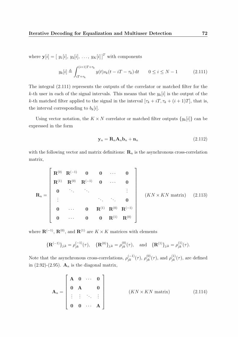
yn = RnAnbn + nn (2.112)
with the following vector and matrix definitions: Rn is the asynchronous cross-correlation
matrix,
Rn =
R(0) R(−1) 0 0 · · · 0
R(1) R(0) R(−1) 0 · · · 0
0. . . . . .
......
. . . . . . 0
0 · · · 0 R(1) R(0) R(−1)
0 · · · 0 0 R(1) R(0)
(KN ×KN matrix) (2.113)
where R(−1), R(0), and R(1) are K ×K matrices with elements
R(−1)j,k = ρ(−1)jk (τ), R(0)j,k = ρ
(0)jk (τ), and R(1)j,k = ρ
(1)jk (τ).
Note that the asynchronous cross-correlations, ρ(−1)jk (τ), ρ
(0)jk (τ), and ρ
(1)jk (τ), are defined
in (2.92)-(2.95). An is the diagonal matrix,
An =
A 0 · · · 0
0 A 0...
.... . .
...
0 0 · · · A
(KN ×KN matrix) (2.114)
Iterative Decoding for Equalization and Multiuser Detection 73
where A is the K ×K diagonal matrix defined in (2.101), and nN is the vector,
nn =[nT [0], nT [1], · · · , nT [N − 1]
]T(KN × 1 vector) (2.115)
For the asynchronous case, the maximum-likelihood receiver computes the likelihood
function L(bn) for all 2KN possible combinations of bn, and then selects the sequence
bn that maximises L(bn). For this case, L(bn) = f(y(t) | bn), and [127]
f(y(t) | bn) = exp
− 1
2σ2
∫ NT+2T
0
[ y(t)− x(t; bn) ]2 dt
, t ∈ [0, NT + 2T ] (2.116)
where
x(t; bn) =K∑k=1
N−1∑i=0
bk[i]Aksk(t− iT − τk), t ∈ [0, NT + 2T ]. (2.117)
Equivalently, the most likely bn also maximises [127]
Ω(bn) = 2
∫ NT+2T
0
x(t; bn)y(t) dt−∫ NT+2T
0
(x(t; bn) )2 dt
= 2bTnAnyn − bTnAnRnAnbn. (2.118)
Once more, the observations enter in the function to be maximised by jointly optimum
decisions on through the matched filter outputs. Therefore, yn is a sufficient statistic for
bn. The vector yn given by (2.112) constitutes a set of sufficient statistics for estimating
the transmitted bits bk[i].
If we adopt a block processing approach, the optimum ML detector must compute
2KN likelihood functions and select the K sequences of length N that corresponds to the
greatest likelihood value. Clearly such an approach is much too complex computationally
to be implemented in practice, especially when K and N are large. An alterative approach
is ML sequence estimation employing the Viterbi algorithm. In order to construct a
sequential-type detector, we make use of the fact that each transmitted symbol overlaps
at most with 2K − 2 symbols. Thus, a significant reduction in computational complexity
is obtained with respect to the block-size parameter N , but the exponential dependence
on K cannot be reduced. It is apparent that the optimum ML receiver employing the
Viterbi algorithm also involves such a high computational complexity that its practical
Iterative Decoding for Equalization and Multiuser Detection 74
use is limited. In the following sections, a number of suboptimum detectors whose
complexity grows linearly with K are considered.
2.7 Linear Multiuser Detectors
The matched filter (conventional detector) has a complexity that grows linearly with the
number of users, K. But susceptibility to MAI from non-orthogonal users means that the
matched filter may make errors even in the absence of noise. In contrast, the optimum
receiver demodulates the data error-free in the absence of noise, but has a computational
complexity that grows exponentially with the number of users, K. In this section, we
consider linear multiuser detectors with computational complexities that grow linearly
with K, but do not exhibit vulnerability to interference from other users.
2.7.1 Decorrelating Detector
Firstly, the case of symbol-synchronous transmission is considered. In this case, the
output of the K matched filters in the i-th code bit interval is represented by the received
signal vector, y[i], given by
y[i] = RAb[i] + n[i] (2.119)
where R, A, b[i], and n[i] are defined in (2.104), (2.101), (2.102), and (2.103), respectively.
Noise vector n[i] has a covariance
En[i]nT [i] = σ2R. (2.120)
Since the noise is Gaussian, y[i] is described by a K-dimensional Gaussian PDF with
mean RAb[i] and covariance R. That is [93],
p(y[i] | b[i]) =1√
(2πσ2)K det Rexp
− 1
2σ2(y[i]−RAb[i])TR−1(y[i]−RAb[i])
(2.121)
Iterative Decoding for Equalization and Multiuser Detection 75
The best linear estimate of b[i], denoted by b0[i], is defined as the value of b[i] that
minimises the likelihood function
L(b[i]) = (y[i]−RAb[i])TR−1(y[i]−RAb[i]), (2.122)
and hence [69],
b0[i] = arg minb[i]
(y[i]−RAb[i])TR−1(y[i]−RAb[i]). (2.123)
The result of this minimisation yields
b0[i] = A−1R−1y[i], (2.124)
and the ML estimates of the detected symbols, bk[i], is given by
bk[i] = sgn
(1
Ak
R−1y[i]
k
)= sgn
( R−1y[i]
k
)for k = 1, . . . , K. (2.125)
Note that the estimate b0[i] is also the best linear estimate that maximises the likelihood
function given by (2.108). Since y[i] = RAb[i] + n[i], it follows from (2.124) that [69]
b0[i] = b[i] + A−1R−1n[i] (2.126)
Therefore, b0[i] is an unbiased estimate of b. The transformation R−1 has eliminated the
interference components between the users, and as a consequence, the near-far problem is
also eliminated. The decorrelating detector is so-called because the linear transformation
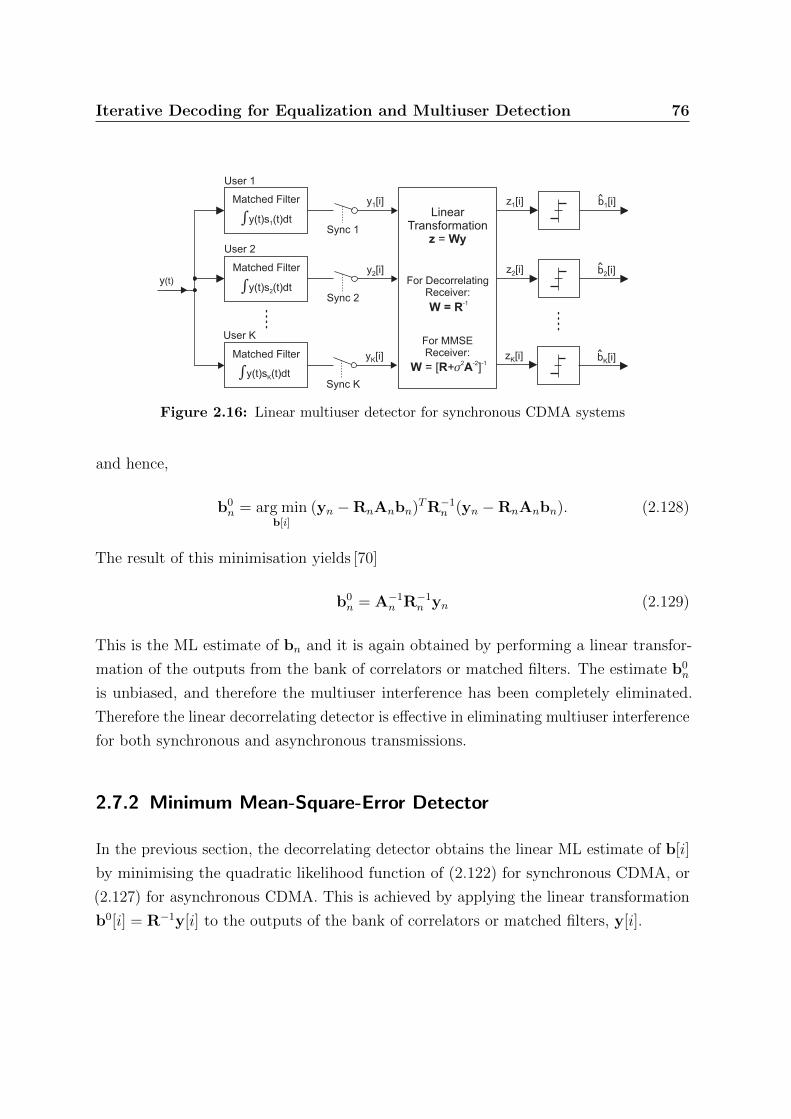
R−1 is used to tune out or decorrelate the multiuser interference. Figure 2.16 illustrates
the receiver structure. The symbol estimates bk[i] are obtained by performing the linear
transformation R−1 on the vector of matched filter outputs y[i], and therefore, the
computational complexity is linear in K.
In asynchronous transmission, the received signal at the output of the matched filters
is given by (2.112). The best linear estimate of bn, denoted by b0n, is the value of bn
that minimises the likelihood function [93]
L(bn) = (yn −RnAnbn)TR−1n (yn −RnAnbn) (2.127)
Iterative Decoding for Equalization and Multiuser Detection 76
W R A= [ + ]s2 -2 -1
W = R-1
LinearTransformation
=z Wy
For DecorrelatingReceiver:
For MMSEReceiver:
z [i]1
z [i]2
z [i]K
y [i]1
y [i]2
y [i]K
y(t)
Matched Filter
Sync 1
User 2
Sync 2
User K
Sync K
b [i]1
b [i]2
b [i]K
òy(t)s (t)dtK
òy(t)s (t)dt1
User 1
Matched Filter
òy(t)s (t)dt2
Matched Filter
Figure 2.16: Linear multiuser detector for synchronous CDMA systems
and hence,
b0n = arg min
b[i]
(yn −RnAnbn)TR−1n (yn −RnAnbn). (2.128)
The result of this minimisation yields [70]
b0n = A−1
n R−1n yn (2.129)
This is the ML estimate of bn and it is again obtained by performing a linear transfor-
mation of the outputs from the bank of correlators or matched filters. The estimate b0n
is unbiased, and therefore the multiuser interference has been completely eliminated.
Therefore the linear decorrelating detector is effective in eliminating multiuser interference
for both synchronous and asynchronous transmissions.
2.7.2 Minimum Mean-Square-Error Detector
In the previous section, the decorrelating detector obtains the linear ML estimate of b[i]
by minimising the quadratic likelihood function of (2.122) for synchronous CDMA, or
(2.127) for asynchronous CDMA. This is achieved by applying the linear transformation
b0[i] = R−1y[i] to the outputs of the bank of correlators or matched filters, y[i].
Iterative Decoding for Equalization and Multiuser Detection 77
Another approach is to seek the linear transformation b0[i] = Wy[i], where the
matrix W is to be determined so as to minimise the mean square error (MSE) [93]:
MSE(b[i]) = EA(b[i]− b0[i])TA(b[i]− b0[i])
= E
(Ab[i]−Wy[i])T (Ab[i]−Wy[i])
(2.130)
where the expectation is with respect to the data vector b[i] and the additive noise
n[i]. The optimum matrix W may be found by forcing the error (b[i]−Wy[i]) to be
orthogonal to the data vector y[i]. Thus
E
(Ab[i]−Wy[i])yT [i]
= 0
EAb[i]yT [i]
−WE
y[i]yT [i]
= 0 (2.131)
Consider the case of synchronous transmission. We have
EAb[i]yT [i] = EAb[i]AbT [i]RT = A2RT (2.132)
and
Ey[i]yT [i] = E
(RAb[i] + n[i])(RAb[i] + n[i])T
= RA2RT + σ2RT (2.133)
By substituting (2.132) and (2.133) into (2.131) and solving for W. We obtain
W =(R + σ2A−2
)−1(2.134)
Therefore, the minimum mean square error (MMSE) estimate of b[i] is [140] [73]
b0[i] = A−1(R + σ2A−2
)−1y[i] (2.135)
and the estimated symbols are obtained by
bk[i] = sgn
(1
Ak
(R + σ2A−2
)−1k
)= sgn
((R + σ2A−2
)−1k
)for k = 1, . . . , K (2.136)
Iterative Decoding for Equalization and Multiuser Detection 78
The MMSE criterion produces a biased estimate of b, hence there is some residual
multiuser interference. Note that in the high-SNR case when σ2 → 0, then
(R + σ2A−2
)−1 → R−1 (2.137)
and the MMSE solution approaches the ML solution in (2.129). In this case, the MMSE
detector becomes equivalent to the decorrelator detector. On the other hand, in the
low-SNR case when σ2A−2 R, then
(R + σ2A−2
)−1 → σ−2A2 (2.138)
and the detector essentially ignores the interference from other users because the additive
noise is the dominant term . In this case the MMSE detector becomes equivalent to
the matched filter detector with amplitude scaling to compensate for the received power
levels. Figure 2.16 illustrates the receiver structure for linear MMSE detector.
Similarly, for asynchronous transmission, the matrix W is chosen so as to minimise
the mean square error (MSE):
MSE(bn) = E
(Anbn −Wyn)T (Anbn −Wyn)
(2.139)
In this case, the optimum choice of W is
W =(Rn + σ2A−2
n
)−1(2.140)
and, hence the MMSE estimate of bn is [140] [73]
b0n = A−1
n
(Rn + σ2A−2
n
)−1yn (2.141)
The output of the MMSE detector is then bn = sgn(b0n).
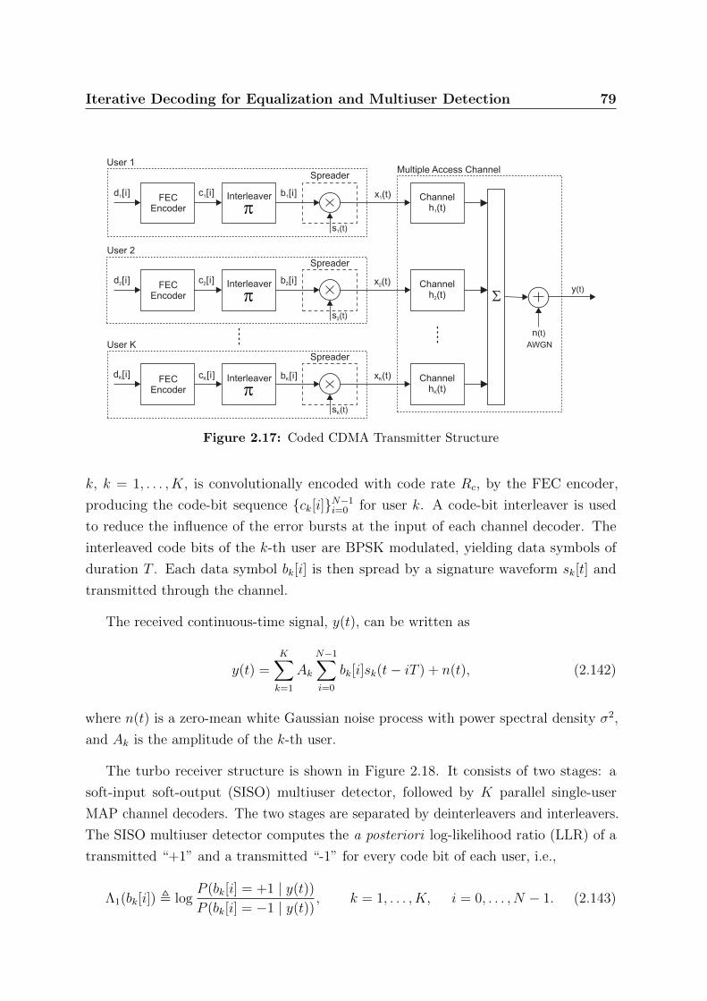
2.8 Turbo Multiuser Detection for Synchronous CDMA
We consider a convolutionally coded synchronous real-valued CDMA system with K
users, employing normalised signature waveforms s1, s2, . . . , sK , and tranmitting through
an additive white Gaussian noise channel. The block diagram of the transmitter structure
for this system is shown in Figure 2.17. The binary data sequence dk[i]M−1i=0 for user
Iterative Decoding for Equalization and Multiuser Detection 79
AWGN
y(t)S
n(t)
Multiple Access Channel
FECEncoder
Interleaver
pChannel
h (t)1
Spreader
s1(t)
d [i]1 c [i]1 b [i]1
FECEncoder
Interleaver
pChannel
h (t)2
Spreader
s2(t)
d [i]2 c [i]2 b [i]2
FECEncoder
Interleaver
pChannel
h (t)K
Spreader
sK(t)
d [i]K c [i]K b [i]K
x (t)1
x (t)2
x (t)K
User 1
User 2
User K
Figure 2.17: Coded CDMA Transmitter Structure
k, k = 1, . . . , K, is convolutionally encoded with code rate Rc, by the FEC encoder,
producing the code-bit sequence ck[i]N−1i=0 for user k. A code-bit interleaver is used
to reduce the influence of the error bursts at the input of each channel decoder. The
interleaved code bits of the k-th user are BPSK modulated, yielding data symbols of
duration T . Each data symbol bk[i] is then spread by a signature waveform sk[t] and
transmitted through the channel.
The received continuous-time signal, y(t), can be written as
y(t) =K∑k=1
Ak
N−1∑i=0
bk[i]sk(t− iT ) + n(t), (2.142)
where n(t) is a zero-mean white Gaussian noise process with power spectral density σ2,
and Ak is the amplitude of the k-th user.
The turbo receiver structure is shown in Figure 2.18. It consists of two stages: a
soft-input soft-output (SISO) multiuser detector, followed by K parallel single-user
MAP channel decoders. The two stages are separated by deinterleavers and interleavers.
The SISO multiuser detector computes the a posteriori log-likelihood ratio (LLR) of a
transmitted “+1” and a transmitted “-1” for every code bit of each user, i.e.,
Λ1(bk[i]) , logP (bk[i] = +1 | y(t))
P (bk[i] = −1 | y(t)), k = 1, . . . , K, i = 0, . . . , N − 1. (2.143)
Iterative Decoding for Equalization and Multiuser Detection 80
Using Bayes’ rule, (2.143) can be rewritten as
Λ1(bk[i]) , logp(y(t) | bk[i] = +1)
p(y(t) | bk[i] = −1)︸ ︷︷ ︸λ1(bk[i])
+ logP (bk[i] = +1)
P (bk[i] = −1)︸ ︷︷ ︸λ2(bk[i])
, (2.144)
where the second term in (2.144), denoted by λ2(bk[i]), represents the a priori LLR of
the code bit bk[i], which is computed by the MAP channel decoder of the k-th user in
the previous iteration, interleaved and then fed back to the SISO multiuser detector. For
the first iteration, assuming equally likely code bits (i.e., no prior information available),
we then have λ2(bk[i]) = 0 for 1 ≤ k ≤ K and 0 ≤ i < N . The first term in (2.144),
denoted by λ1(bk[i]), represents the extrinsic information delivered by the SISO multiuser
detector based on the received signal y(t), the structure of the multiuser signal given by
(2.142), the prior information about the code bits of all the other users, λ2(bl[i])i; l 6=k,and the prior information about the code bits of the k-th user other than the i-th bit,
λ2(bk[j])j 6=i. The extrinsic information λ1(bk[i])i, of the k-th user, which is not
influenced by the a priori information λ2(bk[i])i provided by the MAP channel decoder,
is then reverse interleaved and fed into the k-th user’s channel decoder as the a priori
Iterative Decoding for Equalization and Multiuser Detection 84
where ek denotes a K-vector of all zeros, except for the k-th element, which is 1. Therefore,
bk[i] is obtained from b[i] by setting the the k-th element to zero. For each user, a soft
interference cancellation is performed on the matched filter output y[i] in (2.146), to
obtain
yk[i] , y[i]−RAbk[i]
= RA(b[i]− bk[i]
)+ n[i], k = 1, . . . , K (2.154)
Such a soft inference cancellation scheme was first proposed by Hagenauer [37]. Next,
in order to further suppress the residual interference in yk[i], an instantaneous linear
minimum mean-square error (MMSE) filter wk[i] is applied to yk[i] to obtain
zk[i] = wTk [i]yk[i] (2.155)
where the filter wk[i] ∈ RK is chosen to minimise the mean-square error between the
code bit and the filter output zk[i]:
wk[i] = arg minw∈RK
E(bk[i]−wTyk[i]
)2
= arg minw∈RK
wTEyk[i]y
Tk [i]
w − 2wTE bk[i]yk[i] (2.156)
where using (2.154), we have
Eyk[i]yTk [i] = RA Cov
b[i]− bk[i]
AR + σ2R (2.157)
and
Ebk[i]yk[i] = RA Ebk[i]
(b[i]− bk[i]
)= RAek (2.158)
Substituting (2.157) and (2.158) into (2.156), we have
wk[i] =(RVk[i]R + σ2R
)−1RAek
= AkR−1(Vk[i] + σ2R−1
)−1ek (2.159)
Iterative Decoding for Equalization and Multiuser Detection 85
where Vk[i] is defined as
Vk[i] , ACov
b[i]− bk[i]
A
=K∑j=1j 6=k
A2j
(1− b2
j [i])
ejeTj + A2
kekeTk . (2.160)
Substituting (2.154) and (2.159) into (2.155), we obtain [133]
zk[i] = AkeTk
(Vk[i] + σ2R−1
)−1(R−1y[i]−Abk[i]
). (2.161)
Note that the term R−1y[i] in (2.161) is the output of a linear decorrelating multiuser
detector (Section 2.7.1).
Gaussian Approximation of Linear MMSE Filter Output
The distribution of the residual interference plus noise at the output of a linear MMSE
multiuser detector is well approximated by a Gaussian distribution [89]. Therefore, the
output zk[i] of the instantaneous linear MMSE filter in (2.155) can be modelled as the
output of an equivalent additive white Gaussian noise channel having bk[i] as its input
symbol. This equivalent channel model can be represented as
zk[i] = µk[i]bk[i] + ηk[i], (2.162)
where µk[i] is the equivalent amplitude of the k-th user’s signal at the output and
ηk[i]∼N (0, ν2k [i]) is a Gaussian noise sample. Using (2.154) and (2.155), the parameters
µk[i] and ν2k [i] can be computed as follows,
µk[i] , Ezk[i]bk[i]
= AkeTk
(Vk[i] + σ2R−1
)−1Ebk[i]A
(b[i]− bk[i]
)+ bk[i]n[i]
= A2
k
[(Vk[i] + σ2R−1
)−1]k,k
(2.163)
Iterative Decoding for Equalization and Multiuser Detection 86
and
ν2k [i] , Varzk[i] = Ez2
k[i] − µ2k[i]
= wTk [i]Eyk[i]yTk [i]wk[i]− µ2
k[i]
= µk[i]− µ2k[i] (2.164)
where the expectation is taken with respect to the code bits of interfering users bj [i]j 6=kand the channel noise vector n[i]. Using (2.154) and (2.154), the extrinsic information
delivered by the instantaneous linear MMSE filter is then [133]
λ1(bk[i]) , logp(zk[i] | bk[i] = +1)
p(zk[i] | bk[i] = −1)
= −(zk[i]− µk[i])2
2ν2k [i]
+(zk[i] + µk[i])
2
2ν2k [i]
=2zk[i]
1− µk[i](2.165)
Recursive Procedure for Computing Soft Output
In order to form the extrinsic LLR λ1(bk[i]) at the instantaneous linear MMSE filter,
zk[i] and µk[i] must be computed first (2.165). From (2.161) and (2.163) the computation
of zk[i] and µk[i] involves inverting a K ×K matrix:
Φk[i] ,(Vk[i] + σ2R−1
)−1. (2.166)
This matrix inversion, Φk[i], can computed efficiently using the following recursive
procedure. Define Ψ(0) , (1/σ2)R, and
Ψ(k) ,
(σ2R−1 +
k∑j=1
A2j
(1− b2
j [i])
ejeTj
)−1
, k = 1, . . . , K. (2.167)
Using the matrix inversion lemma, Ψ(k) can be computed recursively as
Ψ(k) = Ψ(k−1) −
1
A−2k
(1− b2
k[i])−1
Ψ(k−1)k,k
(Ψ(k−1)ek) (
Ψ(k−1)ek)T,
k = 1, . . . , K. (2.168)
Iterative Decoding for Equalization and Multiuser Detection 87
Denote Ψ , Ψ(K). Using the definition of Vk[i] given by (2.160), we can then compute
Φk[i] from Ψ as follows [133]:
Φk[i] =(Ψ−1 + A2
kb2k[i]eke
Tk
)−1
= Ψ−
1(Akbk[i]
)−2
Ψk,k
(Ψek) (Ψek)T , k = 1, . . . , K. (2.169)
Finally, the low-complexity SISO multiuser detection algorithm for synchronous CDMA
systems is summarised in Table 2.4.
1. Given the extrinsic information (in LLR form), λ2(bk[i])k, from the FEC
decoders, calculate the soft bit estimates (for k = 1, . . . , K) using:
bk[i] = tanh
(1
2λ2(bk[i]
),
b[i] =[b1[i], · · · , bK [i]
]Tbk[i] = b[i]− bk[i]ek
2. Using the recursive procedure of (2.167), (2.168), and (2.169), calculate
the matrix inversion:
Φ(k) = (Vk[i] + σ2R−1)−1, for k = 1, . . . , K,
3. Perform soft interference cancellation and linear MMSE filtering (for
k = 1, . . . , K) using:
zk[i] = AkeTkΦk[i]
(R−1y[i]−Abk[i]
)4. Calculate the extrinsic information λ1(bk[i])k, for k = 1, . . . , K, using:
λ1(bk[i]) =2zk[i]
1− µk[i]where µk[i] = A2
k Φk[i]k,k
Table 2.4: Algorithm: Low-Complexity Soft MUD for Synchronous CDMA
Iterative Decoding for Equalization and Multiuser Detection 88
Eb/N0 (dB)
Bit E
rror
Rate
10-4
10-3
10-2
10-1
100MMSE-Based Turbo MUD (Synchronous CDMA)
0.0 0.5 1.0 1.5 2.0 2.5 3.0 3.5 4.0
Single User Bound
1 Iteration
2 Iterations
3 Iterations
4 Iterations
5 Iterations
Figure 2.20: Performance of MMSE-based low-complexity turbo MUD: four users (K = 4),equal power, equal cross-correlations (ρ = 0.7); each user employs a rate-1/2constraint-length-5 convolutional code and length-128 interleaver.
Typical performance results show that near-interference-free performance can be
readily achieved when there is sufficient signal-to-noise ratio (SNR) for the initial SISO
MUD to gain useful information about the channel symbols. Figure 2.20 shows an
example of such a result in which there are K = 4 users with equal power and equal cross-
correlations of ρ = 0.7. Each user employs a rate-1/2, constraint-length-5 convolutional
code with a length-128 interleaver. Note that near-single-user performance is achieved
after only five iterations with very moderate SNR.
2.9 Turbo Multiuser Detection for CDMA with
Multipath Fading
In this section, the low complexity SISO multiuser detector for synchronous CDMA
systems (presented in Section 2.8.2) is extended to incorporate asynchronous CDMA
systems with multipath fading channels. This low-complexity SISO multiuser detector
Iterative Decoding for Equalization and Multiuser Detection 89
for asynchronous CDMA systems, which is also based on combined soft interference
cancelation and linear MMSE filtering, was proposed by Li, Wang, and Georghiades [57].
2.9.1 Signal Model and Sufficient Statistics
We consider a K-user asynchronous CDMA system transmitting over multipath fading
channels. The transmitted signal due to the k-th user is given by
xk(t) = Ak
N−1∑i=0
bk[i]sk(t− iT ) (2.170)
where N is the number of data symbols per user per frame; T is the symbol interval;
Ak is the amplitude of the k-th user; bk[i] is i-th transmitted bit of the k-th user; and
sk(t); 0 ≤ t ≤ T is the normalised signature waveform of the k-th user. It is assumed
that sk(t) is supported only on the interval [0, T ] and has unit energy.
The k-th user’s signal xk(t) propagates through a multipath channel with impulse
response
hk(t) =L∑l=1
g′k,l(t)δ(t− τk,l) (2.171)
where L is the number of paths in the k-th user’s channel, and where g′k,l(t) and τk,l
are the complex fading process and the delay of the l-th path of the k-th user’s signal,
respectively. It is assumed that the fading processes are known to the receiver and do
not vary during one coded symbol interval, but may vary from symbol to symbol, i.e.,
g′k,l(t) = g′k,l(iT ) , gk,l[i] for iT ≤ t < (i+ 1)T
The received signal, y(t), is the superposition of the K users’ signals plus the additive
white Gaussian noise, given by
y(t) =K∑k=1
xk(t) ? hk(t) + n(t) (2.172)
=K∑k=1
Ak
N−1∑i=0
bk[i]L∑l=1
gk,l[i]sk(t− iT − τk,l) + n(t) (2.173)
where n(t) is a zero-mean complex AWGN process with power spectral density σ2.
Iterative Decoding for Equalization and Multiuser Detection 90
for i = 0, . . . , N − 1. These a posteriori probabilities are computed using the BCJR
algorithm [6] (from Section 2.3.3) based on the a priori information from the ESE,
λ1(ck[i])i, and knowledge of the code structure.
As in (2.212), Λ2(ck[i]) can be expressed as the sum of extrinsic information λ2(ck[i])
and a priori information λ1(ck[i]). The sequence of extrinsic information, λ2(ck[i])i, is
interleaved (producing λ2(bk[i])i) and fed back to the ESE as a priori information for
the next iteration.
Additionally, the DEC estimates the a posteriori LLRs of the information bits,
Λ2(dk[i])i, and at the final iteration, performs a hard decision on the information bits,
producing dk[i]i .
2.11 Conclusion
In this chapter, the iterative decoding principles from turbo coding were applied to
channel equalization and multiuser detection. The techniques presented will be the
basis for the work described in the following chapters. First, the BCJR MAP algorithm
was introduced for decoding convolutional codes over an AWGN channel. The BCJR
algorithm is a fundamental building block of turbo decoding schemes.
Next, the inter-symbol interference (ISI) channel was presented. For coded data
transmissions, the FEC encoder of the transmitter and the ISI channel can be modelled
as a serial concatenated coding scheme transmitting over a memoryless channel. This
model is similar to a standard serial encoder for turbo coding, and therefore, iterative
decoding techniques can be used at the receiver. Iterative decoding for ISI channels is
known as turbo equalization. Turbo equalization receiver structures were discussed and
performance results presented.
Iterative Decoding for Equalization and Multiuser Detection 104
Finally, the multiple-access channel and multiuser detection using iterative decoding
was presented. For coded data transmissions, the FEC encoder of the transmitter and the
MAI (multiple-access interference) channel can also be modelled as a serial concatenated
coding scheme, and therefore, iterative decoding techniques can be utilised. Iterative
decoding of multiple-access channels is commonly known as turbo MUD. Low-complexity
multiuser detectors for use in turbo MUD receivers were presented for synchronous
CDMA, asynchronous CDMA, and asynchronous IDMA systems.
Chapter 3
IDMA Performance Optimisation using
Variance Transfer Analysis
In this chapter, Variance Transfer (VT) charts are used to analyse and optimise iterative
receiver performance of a multiuser IDMA system. Introduced by Schlegel and Grant
[102], VT charts are similar in concept to Extrinsic Information Transfer (EXIT) charts
[115], but are better suited for analysing multiuser iterative receivers. VT Charts provide
a graphical interpretation of the reliability of information passed between the constituent
components of an iterative receiver. Once the VT characteristic curves have been
determined, receiver performance can be optimised by attempting to closely match the
VT characteristics of the multiuser detector (MUD) and the forward error correction
(FEC) channel decoders. The MUD VT characteristic can be manipulated by the selection
of multiuser detection algorithm and the number of simultaneous users (system load).
The FEC channel decoder VT characteristic can be manipulated by the selection of error
correction code.
Two multiuser system scenarios are considered for optimisation:
Layered IDMA with Power Allocation. Firstly, We extend the IDMA concept to a
multi-rate system where different users transmit data at different rates and the
same low-complexity iterative receiver structure can still be used. High-rate users
are supported by breaking up the input data stream into multiple sub-streams. An
IDMA layer is created from each sub-stream, and the multiple IDMA layers are then
combined and the composite layered signal is transmitted from a single antenna.
The iterative receiver treats each IDMA layer as a virtual user.
105
IDMA Performance Optimisation using Variance Transfer Analysis 106
Chayat et. al. [18] observed that the performance of an iterative receiver is improved
if different users transmit at different powers. This allows the iterative decoder
to operate in an “onion peeling” mode, where the higher-power layers converge
first, decreasing their contribution to the residual noise, and then the lower-power
layers converge. CDMA and IDMA systems utilising iterative receivers can exploit
this power allocation strategy to gain an improvement in performance. Caire
et. al. [17] have shown that this power optimisation problem can be solved by
optimising the partial loads, and developed simple optimisation methods based on
linear programming techniques. In [103], Schlegel et al. applied the work of [18] and
[17] to develop allocation schemes for iterative CDMA receivers that are based on
combined soft interference cancellation and MMSE filtering (i.e., CDMA multiuser
detector schemes of the type described in Section 2.8.2).
To improve the performance of our layered IDMA scheme, we develop a simple power
allocation scheme, where the power levels for each IDMA layer are calculated using
Variance Transfer (VT) analysis and linear programming techniques. In a Rayleigh
flat-fading environment, simulation results demonstrate that the performance of
this proposed system is close to the theoretical limit. This original contribution was
published in [63].
FEC Code Allocation for Dynamic Loads. Secondly, we propose an alternative opti-
misation approach for inducing “onion peeling” operation in the iterative receiver.
Ten Brink [116] demonstrated that different FEC codes generate different FEC
channel decoder VT characteristics. As an alternative to transmit power allocation,
the judicious selection of FEC codes can also be used to match the receiver VT
characteristics for optimal performance.
A simple FEC code allocation strategy for multiuser systems with dynamic loads
is devised. New users are allocated FEC codes according to the existing system
load, which allows the FEC decoder VT curve to dynamically match the MUD
VT curve as it changes with system load, providing optimal system performance
over a range of operating conditions. We derive a numerical method for optimising
performance based on FEC code allocation, and present simulation results. For
small multiuser systems, results demonstrate that the performance of the proposed
system approaches the theoretical single user bound. This original contribution was
published in [65].
IDMA Performance Optimisation using Variance Transfer Analysis 107
3.1 Variance Transfer Charts and Analysis
s2
n
ElementarySignal
Estimator userk
dk[ i ]Soft FECChannelDecoder
User k
ESE outputvariance
l1(b )k[ i ] l1(c )k[ i ]
l2(b )k[ i ] l2(c )k[ i ]Interleaver
Deinterleaver
pk-1
pkg( )
vardec
varese
vardec
x (t) hK K
S
n(t)
Multiple Access Channel
y(t)
x (t) h1 1
x (t) h2 2
ESE inputvariance
DEC outputvariance
f( )
varese
DEC inputvariancechannel
noisevariance
Figure 3.1: Variance transfer between constituent iterative receiver components
The Variance Transfer (VT) chart method [102] analyses the transfer functions of the
multiuser detector and the channel decoders in order to predict the behaviour of the
iterative receiver. Figure 3.1 shows the variance transfer paths for the IDMA iterative
receiver from Section 2.10.2. There are two VT functions:
• The ESE VT function is defined as the variance in the ESE output, varese, as a
function of the error variance in the soft-bit estimates from the FEC decoders,
vardec,k, and the channel noise variance, σ2n, i.e., varese = f(vardec,k , σ
2n)
• The FEC channel decoder (DEC) VT function is defined as the variance in the k-th
user DEC output, vardec,k, as a function of the estimation error variance from the
ESE, varese, i.e., vardec,k = g(varese)
3.1.1 ESE Variance Transfer Function
For our IDMA system, the multiuser interference is proportional to the system load,
β, and the variance of the estimation error, vardec,k. The system load is defined as the
ratio of users, K, to bandwidth expansion, R, (i.e. β = K/R), and the estimation error
variance is defined as
vardec,k = E
(ck[i]− ck[i])2 (3.1)
We first consider the case of equal power for all users, Pk = P . For this case, the
estimation error for all users will be equal, vardec,k = vardec. For the ESE, the expression
IDMA Performance Optimisation using Variance Transfer Analysis 108
for the residual multiple access interference plus channel noise at the input to the FEC
decoder is given by
varese( vardec ) =
(K − 1
R
)P vardec + σ2
n
= limK→∞
βP vardec + σ2n (3.2)
where σ2n is the channel noise, and the soft FEC decoder estimation error variance,
vardec , is the average power of the residual symbol interference. Therefore, given vardec ,
equation (3.2) describes the noise variance in the input signal to the FEC decoder for the
next iteration. Figure 3.2a shows the ESE VT function (3.2) for a typical IDMA system.
0.0 0.2 0.4 0.6 0.8 1.0
Cancelled Symbol Variance
Sin
gle
-User
Nois
e L
evel
ChannelNoiseLevel
Slope:System Load
0.0
0.5
1.0
1.5
2.0
2.5
3.0
3.5Variance Transfer: ESE Interference Canceller
DecreasingSystemLoad
IncreasingSystemLoad
(a) ESE interference canceller
Input N
ois
e V
ariance
0.0 0.2 0.4 0.6 0.8
3.5
3.0
2.5
2.0
1.5
0.5
1.0
0.0
1.0
Soft-Bit (FEC Decoder) Variance
Variance Transfer: FEC Decoder
Turbo Code
Conv. Code (v=2)
Repetition Code
Conv. Code (v=3)
Conv. Code (v=4)
(b) FEC decoder
Figure 3.2: Variance transfer functions for (a) ESE interference canceller, and (b) FECdecoder (for various 1/3-rate codes)
The more accurate the symbol estimates of the other interfering users, the smaller the
residual noise that the error control decoder has to overcome. But even if the interfering
symbols are known exactly, the FEC decoder still has to overcome the AWGN channel
noise.
IDMA Performance Optimisation using Variance Transfer Analysis 109
3.1.2 FEC Decoder Variance Transfer Function
At the input of the k-th soft FEC decoder, the input sequence has an additive Gaussian
noise distortion with associated variance varese per symbol. Therefore the decoder can
be analysed in the same manner as an AWGN channel. The output of the decoder are
the soft bit estimates, and the primary measure of their reliability is the variance vardec.
Unfortunately, no closed form expression exists for vardec as a function of varese other than
for very simple codes. The VT functions vardec = g(varese) are found using numerical
methods by simulating the input-output behaviour of the FEC code. Figure 3.2b shows
the VT functions for a repetition code, best known convolutional codes (with constraint
lengths, v, of 2, 3, and 4) [54], and a turbo code [12]. All the codes shown have a rate of
1/3.
3.1.3 Example Variance Transfer Chart
0.0
0.5
1.0
1.5
2.0
2.5
3.0
0.0 0.2 0.4 0.6 0.8 1.0
Soft-Bit (FEC Decoder) Variance
Re
sid
ua
l E
SE
Inte
rfe
rence V
aria
nce
(0)
(1)
(2)
Noise Limitation
InterferenceLimitation
(12)
(3)
ConvergenceTunnel
3.5
Variance Transfer Chart36 Users, Common FEC Code, Equal Tx Power, Eb/N0 = 10dB
Soft FEC Decoder
Soft Interference Canceller
Receiver Iterations
Figure 3.3: Variance transfer chart for an IDMA system with 36 users using equal transmitpower and a common FEC code (Eb/N0 = 10dB)
Figure 3.3 shows a VT chart for our IDMA system with all users transmitting at
equal power, and a receiver Eb/N0 value of 10dB. Decoding starts at point (0) where
IDMA Performance Optimisation using Variance Transfer Analysis 110
the FEC decoders have to work with full interference and noise. After the first iteration,
the receiver reduces the interference by subtracting estimates of the interfering signals,
this leads to point (1). The vertical distance between point (0) and point (1) is the
resultant reduction in noise variance at the input of the soft-output FEC decoder. In the
next iteration, the noise variance can be further reduced to point (2), and so on, until
the iterations reach the intersection point between the two curves, point (12). At this
point virtually all the interference has been canceled, and only channel noise is left. The
performance of the individual decoders at this point is essentially that of the decoders in
Gaussian noise, and is known as the noise limitation fix point of the iterative decoder.
In Figure 3.3, note that along the iterative trajectory there is a section which forms a
narrow channel through which the trajectory progresses in small steps. This area is the
interference limitation. An increase in the system load, or reduction in Eb/N0 ratio will
create another intersection point between the two VT curves (within this interference
limitation region), and the variance will stop improving at this interference limitation fix
point, rather than at the noise limitation fix point. Under these conditions, the decoder
does not function due to an excessive system load. As the load decreases, or the Eb/N0
ratio increases, the channel opens up and convergence to the noise limitation fix point
is suddenly enabled. This effect happens at a sharp Eb/N0 threshold, and gives rise to
the abrupt, cliff-like behaviour of the error rate performance in iterative receivers. This
bound on the VT curve allows us to derive the optimal parameters for our IDMA system
in order to optimise system performance.
Figure 3.4 demonstrates the iterative receiver operating modes and the effect of
Eb/N0 on performance. Figure 3.4a shows the VT for an Eb/N0 of 1.5dB, the receiver
is interference limited and the BER performance is poor regardless of the number of
iterations. Figure 3.4b shows the VT for a slightly higher Eb/N0 of 3.0dB, here the
receiver is no longer interference limited, but “bottlenecked”. Convergence is slow and a
large number of iterations are required to achieve good BER performance. Figure 3.4c
shows that at the higher Eb/N0 of 4.5dB, the bottleneck region has been opened up
and convergence is achieved quickly with only a small number of iterations required to
achieve good BER performance. These operating regions are also reflected in the BER
graph in Figure 3.4d.
IDMA Performance Optimisation using Variance Transfer Analysis 111
0.0
0.5
1.0
1.5
2.0
2.5
3.0
3.5
0.0 0.2 0.4 0.6 0.8 1.0
Soft-Bit Variance
Input N
ois
e V
ariance
FEC Soft Decoder
Soft Interference Cancellation
Receiver Iterations
VT Chart: Interference Limited (Eb/N0 = 1.5dB)
InterferenceLimitation
(0)
(1)
(2)(3)
(a) VT at Eb/N0 = 1.5dB
0.0
0.5
1.0
1.5
2.0
2.5
3.0
0.0 0.2 0.4 0.6 0.8 1.0
Soft-Bit Variance
Input N
ois
e V
ariance
3.5
VT Chart: Slow Convergence (Eb/N0 = 3.0dB)
NoiseLimitation
Bottleneck Region(Slow Convergence)
(0)
(1)
(2)
(3)(4)
(12)
(13)
(14)
FEC Soft Decoder
Soft Interference Cancellation
Receiver Iterations
(b) VT at Eb/N0 = 3.0dB
0.0
0.5
1.0
1.5
2.0
2.5
3.0
3.5
0.0 0.2 0.4 0.6 0.8 1.0
Soft-Bit Variance
Input N
ois
e V
ariance
VT Chart: Fast Convergence (Eb/N0 = 4.5dB)
NoiseLimitation
Wide-Open Region(Fast Convergence)
(0)
(1)
(2)
(3)
(6)
(7)
FEC Soft Decoder
Soft Interference Cancellation
Receiver Iterations
(c) VT at Eb/N0 = 4.5dB
Eb/N0 (dB)
Bit E
rror
Rate
10-4
10-3
10-2
10-1
100
IDMA: Effect of Receiver Iterations
4.50.5 1.0 1.5 2.0 2.5 3.0 3.5 4.0
15 Iterations
1 Iteration
2 Iterations
3 Iterations
4 Iterations
5 Iterations
(d) BER Performance
Figure 3.4: Variance transfer charts demonstrating iterative receiver operating modes: (a)interference limited; (b) slow convergence; and (c) fast convergence.
3.2 Multi-Rate IDMA with Power Allocation
We extend the IDMA multiple-access system (from Section 2.10) to a multi-rate system
where different users transmit data at different rates and the same low-complexity
iterative receiver structure can still be used. High-rate users are supported by breaking
up the input data stream into multiple sub-streams. An IDMA layer is created from
IDMA Performance Optimisation using Variance Transfer Analysis 112
each sub-stream, and the multiple IDMA layers are then combined and the composite
layered signal is transmitted from a single antenna.
InterleaverFECEncoder
dk,1 SymbolMapper
bk,1xk,1
pk,1
High-Rate Tx - User k
ck,1pk,1
InterleaverFECEncoder
dk,J SymbolMapper
bk,Jxk,J
pk,J
ck,J
pk,J
dk
S
P
Tx
xk
Figure 3.5: Transmitter Structure for the Multi-Rate IDMA System
Figure 3.5 shows the transmitter structure for multi-rate users of the multiple-access
scheme. For the high-rate user, a serial-to-parallel converter breaks up the input data
stream is into J sub-streams. An IDMA layer is created from each sub-stream, and the
multiple layers are then combined and transmitted from a single antenna. Each layer
is of equal rate, but unequal power. In order to achieve optimal receiver performance,
transmit power is allocated to the various IDMA layers in accordance to the strategy
developed in Section 3.2.1.
ElementarySignal
Estimator(ESE)
Rx
l1(b )k,1
Soft FECChannelDecoderInterleaver
Deinterleaver
userk
dk,1
dk,J
pk,1-1
pk,1
Soft FECChannelDecoderInterleaver
Deinterleaver
pk,J-1
pk,J
L2(c )k,1
l1(c )k,1
l2(c )k,1
L1(b )k,1
l2(b )k,1
L1(b )k,J
l2(b )k,J
l1(b )k,J l1(c )k,J
L2(c )k,Jl2(c )k,J
S
P
dk
Decoder - User k
Figure 3.6: Receiver Structure for the Multi-Rate IDMA System
Figure 3.6 shows the receiver structure for the multi-rate IDMA system. The iterative
receiver operates as described in Section 2.10.2 and each IDMA layer is treated as a virtual
user. After the receiver has decoded the data for each virtual user, a parallel-to-serial
IDMA Performance Optimisation using Variance Transfer Analysis 113
converter recombines the IDMA layers into the appropriate high-rate streams for each
multi-rate user.
3.2.1 Transmit Power Allocation
Chayat et. al. [18], observed that differences in received power levels are beneficial to the
operation of the joint iterative decoder, and that in practice, only a few different power
levels are needed to achieve good performance.
We develop a power allocation scheme to improve the performance of our layered
IDMA system based on the methods from [102]. First, we extend the VT chart method
to the case of unequal received power levels. Denote σ2ι as the error variance in the ESE
output, varese, at iteration ι. The residual interference and noise variance of an arbitrary
user, at iteration ι, is given by
σ2ι =
1
R
K∑k=1
Pk g
(σ2ι−1
Pk
)+ σ2
n (3.3)
where g( · ) is VT function of the FEC decoder (Section 3.1.2). In the case where the
users are grouped into J power groups, we find
σ2ι =
J∑j=1
KjPjR
g
(σ2ι−1
Pk
)+ σ2
n (3.4)
where Kj, is the number of users in group j. Since different users now contribute with
different received power levels, we need to consider the average system load. The average
system load is defined as βav =∑J
j=1 βjPj. We now obtain
σ2ι = βav
∑ βjPjβav
g
(σ2ι−1
Kj
)+ σ2
n
= βav gav(σ2ι−1) + σ2
n (3.5)
where gav(σ2ι−1) is an average variance transfer function. It is obtained by weighing the
individual code VT functions by the weight factor βPj/βav (composed of their loads and
powers). Equation (3.5) can be visualised and charted in a similar manner as the equal
power case, where the FEC VT function of the code in the equal power case corresponds
to the composite FEC VT function gav( · ) in the unequal power levels case.
IDMA Performance Optimisation using Variance Transfer Analysis 114
If we assume that there are J different power levels, each with a partial load βj , then
the power levels can be optimised using numerical techniques. The number of levels J
is arbitrary and determines the complexity of the numerical method. Caire et. al. [17]
observed that the power optimisation problem can be solved by optimizing the partial
loads. This turns the optimisation into a well-known linear programming problem.
Using the residual recursive interference equation (3.4),
σ2ι =
J∑j=1
KjPjR
g
(σ2ι−1
Pj
)+ σ2
n = f(P, β, z = σ2ι−1) (3.6)
where P = (P1, . . . , PJ), and β = (β1, . . . , βJ). The condition that the VT curves of the
FEC decoders and the ESE do not intersect can be reformulated as
f(P, β, z) < z; z ∈ [σ2min,∞] (3.7)
where the lower limit σ2min is an arbitrary limit dictated by some minimal performance
criterion. In this case we use the error probability of the lowest power level group as
the performance criterion. Given the power Pj and the error control codes used, we
can calculate the maximum tolerable error variance σ2min and (3.7) ensures that no
intersection point exist for larger residual interference variances, therefore enforcing this
minimal performance criterion. This results in the following optimization problem:
minimiseJ∑j=1
βjPj subject to:
f(P,β, z) ≤ z − ε∑J
j−1 βj = β
βj ≥ 0
(3.8)
where z ∈ [σ2min,∞]. The optimisation criterion in (3.8) minimises the average Eb/N0,
which is equivalent to optimising the system load of a given average Eb/N0. The parameter
ε controls the width of the convergence tunnel and ensures that there is a sufficient
opening for the iterations to proceed through. A wider convergence tunnel allows for
faster convergence, but at the cost of a decreased system load. Equation (3.8) becomes a
linear optimisation problem which can be solved by numerical techniques.
We consider the optimisation problem for a high-rate transmitter with 3 IDMA layers.
Figures 3.7a & 3.7b both show the VT charts for 3 equal-sized power groups. Figure 3.7a
uses a FEC code consisting of a 1/3-rate convolutional code serially concatenated with
IDMA Performance Optimisation using Variance Transfer Analysis 115
0.0
1.0
2.0
3.0
4.0
5.0
6.0
7.0
8.0
9.0
0.0 0.2 0.4 0.6 0.8 1.0
Soft-Bit (FEC Decoder) Variance
Re
sid
ua
lE
SE
Va
ria
nce
(Effe
ctive
)
Variance Transfer:Different Tx Power Levels, Conv. Code (CC) FEC
10.0
Interference Cancellation
FEC CC: P (= 1.00 x P)1
FEC CC: P (= 0.50 x P)2
FEC CC: P (= 0.25 x P)3
Combined FEC Code
(a) Convolutional code
Variance Transfer:Different Tx Power Levels, Turbo Code (TC) FEC
0.0
1.0
2.0
3.0
4.0
5.0
6.0
7.0
8.0
9.0
10.0
0.0 0.2 0.4 0.6 0.8 1.0
Soft-Bit (FEC Decoder) Variance
Re
sid
ua
lE
SE
Va
ria
nce
(Effe
ctive
)
Interference Cancellation
FEC TC: P (= 1.00 x P)1
FEC TC: P (= 0.50 x P)2
FEC TC: P (= 0.25 x P)3
Combined FEC Code
(b) Turbo code
Figure 3.7: VT charts for layered-IDMA with power allocation using (a) convolutional codeFEC, and (b) turbo code FEC
a 1/6-rate repetition code. Figure 3.7b uses 1/3-rate turbo code concatenated with
a 1/6-rate repetition code. In both cases, the optimal power levels are found to be
P1 = 0.25×P, P2 = 0.50×P , and P3 = 1.00×P .
Note that the optimisation strategy does not take into account the physical constraints
of the transmitter power amplifier (e.g., power budget and dynamic range). However,
the optimisation results are pleasing in that the optimal power levels do not make any
untoward demands on the underlying physical hardware and the scheme could be readily
implemented using standard transmitter components.
3.2.2 Simulation Results
The simulations assume the receiver has perfect channel knowledge. The system is
evaluated for fast time-varying Rayleigh flat-fading channels where the individual user
channels are independent and uncorrelated.
Figure 3.8a compares the average bit error rate (BER) for 3 high-rate users after
12 receiver iterations versus the signal to noise ratio (SNR) Eb/N0 for layered-IDMA
with and without power allocation, and with 2 types of FEC code (convolutional code,
IDMA Performance Optimisation using Variance Transfer Analysis 116
and turbo code). For Eb/N0 values of 4 dB and greater we observe a performance
improvement of 0.5dB to 1.0dB for layered IDMA with power allocation when compared
to the equal power case. We also observe a modest improvement (of 0.25dB to 0.5dB)
when comparing IDMA with Turbo code FEC against IDMA with convolutional code
FEC.
Figure 3.8b compares the average bit error rate (BER) for 9 high-rate users after
12 receiver iterations versus the signal to noise ratio (SNR) Eb/N0 for layered-IDMA
with and without power allocation, and with 2 types of FEC code (convolutional code,
and turbo code). For Eb/N0 values of 4 dB and greater we observe a performance
improvement of 0.5dB to 1.0dB for layered IDMA with power allocation when compared
to the equal power case. We also observe minimal difference between IDMA with Turbo
code FEC against IDMA with convolutional code FEC.
3.3 FEC Allocation for Dynamic System Loads
From Figure 3.3 we observe that for good system performance, we need to match the
FEC decoder VT curve to ESE VT curve, such that the FEC decoder VT curve is always
above the ESE VT curve (maintaining an acceptable convergence tunnel width), and
only crossing the ESE VT curve at the noise limitation fix point. From Figure 3.2b we
observe that strong FEC codes are a good match for light system loads, and that weaker
FEC codes are a better match for heavier system loads.
We consider a system consisting of a number of persistent users (primary users) and a
number of intermittent users (secondary and tertiary users, where the tertiary users are
more sporadic that the secondary users). From our observations, we hypothesise that the
optimal FEC code allocation strategy is for assign strong FEC codes to primary users,
and increasingly weaker FEC codes to the secondary and tertiary users. The composite
FEC decoder VT function would be dominated by the strong codes at light loads, and
dominated by the weaker codes at heavy loads. We now develop optimisation techniques
to test our hypothesis
Caire et. al. [17] observed that the power optimisation problem can be solved by
optimising the partial loads, and developed simple optimisation methods based on well-
known linear programming techniques. This optimisation method splits the system
load into a number of sub-groups (or partial loads), where each sub-groups represents
IDMA Performance Optimisation using Variance Transfer Analysis 117
Bit E
rror
Rate
10-3
10-2
10-1
100
Layered IDMA: Effect of Power Allocation (9 Virtual Users)
Eb/N0 (dB)
10-4
0 2 4 6 8 10
Single User Bound
Power Allocation, Turbo Code
Powe Allocation, Conv. Code
Equal Power, Turbo Code
Equal Power, Conv. Code
(a) 3 Users with 3-Layers/User
Bit E
rror
Rate
10-3
10-2
10-1
100
Layered IDMA: Effect of Power Allocation (36 Virtual Users)
Eb/N0 (dB)
10-4
0 2 4 6 8 10
Single User Bound
Power Allocation, Turbo Code
Power Allocation, Conv. Code
Equal Power, Turbo Code
Equal Power, Conv. Code
(b) 12 Users with 3-Layers/User
Figure 3.8: Effect of power allocation on layered IDMA Performance for (a) 3 Users with3-Layers/User; and (b) 12 Users with 3-Layers/User.
IDMA Performance Optimisation using Variance Transfer Analysis 118
a different power level. These sub-groups can be optimised using numerical techniques.
The number of sub-groups (power levels) is arbitrary and determines the complexity of
the numerical method.
Adapting the optimisation techniques from [17], we develop a simple method for FEC
code allocation that optimises the overall system performance.
Denote σ2ι as the error variance in the ESE output, varese, at iteration ι. The residual
interference and noise variance of an arbitrary user, at iteration ι, is given by
σ2ι =
1
R
K∑k=1
P gk
(σ2ι−1
Pk
)+ σ2
n (3.9)
where gk( · ) is the VT function of the FEC decoder for user k (Section 3.1.2). In the
case where the users are grouped into J FEC code groups (each group uses a different
FEC code), we find
σ2ι =
J∑j=1
KjP
Rgj
(σ2ι−1
P
)+ σ2
n (3.10)
where Kj, is the number of users in group j. Since different users now contribute with
different FEC code VT functions, we consider the average system load. The average
system load is defined as βav =∑J
j=1 βjgj( · ). We now obtain
σ2ι = βav
∑ βjP
βavgj
(σ2ι−1
Kj
)+ σ2
n
= βav gav(σ2ι−1) + σ2
n (3.11)
where gav(σ2ι−1) is the average VT function, which is obtained by weighing the individual
code VT functions by the weight factor βj/βav (composed of their loads). Equation (3.11)
can be graphed in a similar manner as the common FEC code case, where the FEC VT
function of the code in the common code case corresponds to the composite FEC VT
function gav( · ) in the multiple code groups case.
The residual recursive interference equation, (3.10), can be restated as
σ2ι = f
(g(σ2ι−1
P), β, z = σ2
ι−1
)(3.12)
IDMA Performance Optimisation using Variance Transfer Analysis 119
where g( · ) = (g1( · ), . . . , gJ( · )), and β = (β1, . . . , βJ). By choosing the maximum error
probability as the minimum performance criterion, the condition that the VT curves of
the FEC decoders and the ESE do not intersect can be reformulated as the following
linear optimisation problem:
minimiseJ∑j=1
βjPgj( · ) subject to:
f(g(
σ2ι−1
P), β, z) ≤ z − ε∑J
j=1 βj = β
βj ≥ 0
(3.13)
where z ∈ [σ2min,∞], and σ2
min is the arbitrary lower limit dictated by the minimal
performance criterion. The optimisation criterion in (3.13) minimises the average Eb/N0,
which is equivalent to optimising the system load of a given average Eb/N0. The parameter
ε controls the width of the convergence tunnel and ensures that there is a sufficient
opening for the iterations to proceed through. A wider convergence tunnel allows for
faster convergence, but at the cost of a decreased system load. Equation (3.13) can be
solved by numerical techniques.
We consider the optimisation problem for an IDMA system with 8 primary users
(always present), 8 secondary users and 16 tertiary users (where the secondary and tertiary
users are intermittent users, the tertiary users are more sporadic than the secondary
users). To minimise the complexity of the optimisation problem, we consider an allocation
of 3 FEC codes (one code for each user group). Each of the following candidate codes are
considered for optimisation: convolutional codes with constraint lengths,v, of 2, 3, 4, 5,
and 6; and turbo codes with RSC encoders of constraint lengths 2 and 3. All candidate
codes are rate 1/3.
The optimal FEC code allocation for the three user groups are found to be turbo code
(with RSC encoders of constraint length 2) for the primary user group; convolutional
code with constraint length of 3 for the secondary user group; and convolutional code
code with constraint length of 2 for the tertiary user group.
We also consider the optimisation problem for an IDMA system where FEC code
allocation is not used, and all 32 users (8 primary, 8 secondary, and 16 tertiary) employ
the same FEC code. Using the same candidate group of codes, the optimal FEC code is
found to be the convolutional code with constraint length of 3.
IDMA Performance Optimisation using Variance Transfer Analysis 120
3.3.1 Simulation Results
The simulations assume the receiver has perfect channel knowledge. The system is
evaluated for fast time-varying Rayleigh flat-fading channels where the individual user
channels are independent and uncorrelated.
We consider the scenario of an IDMA system with up to 32 simultaneous users
(consisting of 8 primary users, which are always present; 8 secondary users; and 16
tertiary users, where the secondary and tertiary users are intermittent users, and the
tertiary users are more sporadic than the secondary users). We compare the performance
of a system employing FEC code allocation against a system using a common FEC code
for all users (in this latter case, the FEC code is a convolutional code with constraint
length of 3, which was found to be the optimal code for a 32-user system without code
allocation).
Figure 3.9a compares the average bit error rate (BER) for 9 users after 12 receiver
iterations versus the signal to noise ratio (SNR) Eb/N0 for an IDMA system with and
without FEC code allocation. For Eb/N0 values of 4 dB and greater we observe a
performance improvement of up 0.5dB to 0.8dB for IDMA with FEC code allocation
when compared to the standard FEC code case. We also observe that performance of
the IDMA system with FEC code allocation is generally within 0.5dB of the single user
bound.
Figure 3.9b compares the average BER for 16 and 32 users after 12 receiver iterations
versus the SNR Eb/N0 for an IDMA system with and without FEC code allocation. For
Eb/N0 values of 4 dB and greater, with 16 users, we observe a performance improvement
of approximately 0.5dB to 1.0dB for IDMA with FEC code allocation when compared to
the standard FEC code case. For 32 users, we observe a modest performance improvement
of approximately 0.3dB when comparing FEC code allocation against standard FEC
code case.
3.4 Conclusion
The analysis of iterative multiuser receiver performance using Variance Transfer (VT)
analysis has been presented. It was shown that receiver performance is optimal when
the VT characteristics of the constituent components are “matched”. Using linear
programming techniques, allocation schemes for transmitter power and FEC codes were
IDMA Performance Optimisation using Variance Transfer Analysis 121
Bit E
rror
Rate
10-3
10-2
10-1
100
IDMA: Effect of FEC Code Allocation (8 Users)
Eb/N0 (dB)
10-4
0 2 4 6 8 10
Single User Bound
8 Users, FEC Code Allocation
8 Users, No FEC Allocation
(a) 8 simultaneous users
Bit E
rror
Rate
10-3
10-2
10-1
100
IDMA: Effect of FEC Code Allocation (16 & 32 Users)
Eb/N0 (dB)
10-4
0 2 4 6 8 10
Single User Bound
16 Users, FEC Code Allocation
16 Users, No FEC Code Allocation
32 Users, FEC Code Allocation
32 Users, No FEC Code Allocation
(b) 16 and 32 simultaneous users
Figure 3.9: Effect of FEC allocation on IDMA performance for (a) 8 simultaneous users; and(b) 16 and 32 simultaneous users
IDMA Performance Optimisation using Variance Transfer Analysis 122
developed to achieve optimal system performance. Two multiuser system scenarios were
considered for optimisation.
First, a multi-rate multiuser scheme using the layered-IDMA with power allocation
was presented and compared with a layered scheme without power allocation (equal
power). The layered IDMA scheme with power allocation was shown to provide superior
performance at moderate and high SNR levels while using the same low-complexity
iterative decoding receiver structure as the other IDMA schemes. In a Rayleigh flat-
fading environment, simulation results show that for Eb/N0 values of 6dB and greater,
the performance of layered IDMA system with power allocation is within 0.5dB of the
single user bound.
Second, an IDMA multiuser scheme employing FEC code allocation for dynamic
loads was presented and compared with a IDMA scheme without FEC code allocation
(all users employ the same FEC code). The IDMA scheme with FEC code allocation was
shown to provide superior performance at moderate and high SNR levels while using the
same low complexity iterative decoding receiver structure as the other IDMA schemes.
In a Rayleigh flat-fading environment, simulation results show that for Eb/N0 values of
6.5dB and greater, the performance of the IDMA system with FEC code allocation and
32 simultaneous users is within 0.7dB of the single user bound.
Chapter 4
Optimal Space-Time Coding using the
Golden Code
In recent years, multiple antenna systems (commonly referred to as multi-input multi-
output or MIMO systems) have proven to be an effective method for realising high-rate
reliable wireless communications. Research in MIMO systems has generally focused on
providing either higher-rate or increased diversity over traditional single antenna (SISO)
systems.
Foschini [30] introduced the layered space-time (BLAST) architecture where a high
throughput rate is achieved by using multiple transmit antennas to transmit multiple
independent data sub-streams in parallel. Multiple receive antennas and multi-user
detection algorithms are used at the receiver end to separate and decode the individual
sub-streams. Although providing high-rate, BLAST has the shortcoming that it does not
provide diversity gain as each data symbol is only transmitted once from one antenna.
Alamouti [3] introduced a simple orthogonal space time block code (STBC) that
provided diversity gain for 2× 1 and 2× 2 multi-antenna systems. This scheme was
generalised and extended by Tarokh et. al. [113] to include higher-dimension MIMO
systems, using real and complex orthogonal STBCs. Although providing diversity gain,
orthogonal STBCs have the shortcoming that (with the exception of a few sporadic
codes) the coding rate does not exceed 1/2.
A generalised class of space-time codes that encompassed both orthogonal STBCs and
BLAST architectures was proposed by Hassibi and Hochwald [39]. This generalised class
of codes, which are known as linear dispersion (LD) codes, are defined as codes that break
up the input data stream into sub-streams that are dispersed in linear combinations over
123
Optimal Space-Time Coding using the Golden Code 124
space and time. Theoretically, LD codes can provide both diversity gain and high-rate.
In general, LD codes can outperform their orthogonal STBC and BLAST sub-classes.
Sethuraman et. al. [105] proposed a methodology for designing full-diversity high-rate
LD codes using cyclic division algebras. A division algebra is used to provide a structured
set of invertible matrices to construct LD space-time codes. Using this technique, Belfiore
et. al. [7] developed the Golden Code, a 2× 2 LD code that provides both diversity gain
and full-rate.
In the first part of this chapter, we investigate the effect of Doppler spread on the
performance of the 2× 2 Golden Code single-user system. Doppler spread is a measure of
spectral broadening caused by the relative motion between the transmitter and receiver
antennas or by the movement of reflecting objects in the channel. Doppler spread is an
important consideration in the design of mobile communication systems.
The decoding methodology for the Golden code is presented, followed by performance
comparisons with the Alamouti code and V-BLAST in Rayleigh fading environments
with Doppler spread. Simulation results show that the Golden Code outperforms both
the Alamouti code and V-BLAST at high SNR levels. For a symbol error rate of 10−4
the Eb/N0 requirement for the Golden code is 5dB less than the Alamouti code and
V-BLAST. This original contribution was published in [60].
The second part of this chapter considers the multiuser case, and we develop a MIMO
framework for IDMA that can provide both diversity gain and high-rate.
Recently multiuser MIMO-IDMA has been proposed [81], where IDMA has been
generalised to multiple antenna systems where users employ V-BLAST (vertical-encoded
layered space time) spatial multiplexing to achieve higher data rates. Decoding is still
performed by an iterative receiver whose complexity is linear in the number of users. We
further extend the MIMO-IDMA concept from IDMA with V-BLAST spatial multiplexing
to IDMA with linear dispersion (LD) codes.
In particular, we investigate the performance of the MIMO-IDMA using the Golden
Code. The Golden Code (GC), is 2× 2 LD code derived from cyclic division algebra
that provides both diversity gain and full-rate [7]. We compare the performance of this
GC-IDMA scheme against MIMO-IDMA schemes employing the Alamouti code and
V-BLAST, and also against the single-user bound. In a Rayleigh flat-fading environment,
simulation results show that GC-IDMA outperforms both Alamouti- and V-BLAST-
IDMA at moderate and high SNR levels. For signal to noise ratios of 8dB and greater,
Optimal Space-Time Coding using the Golden Code 125
the GC-IDMA scheme employing 16 users approaches within 0.25dB of the single-user
bound. This original contribution was published in [62].
4.1 Single-User MIMO System Model
The system model for a multiple-antenna communications system with N transmit and
M receive antennas is shown in Figure 4.1.
Tx1
STBCMapper
TxN
inputsymbols
h11
hNM
Rx1
RxM
hN1
h1M
recoveredsymbols
ChannelEstimator
&SymbolDetectorx
N(i)
y1(i)
nM(i)
AWGN
AWGN
x1(i)
yM(i)
n1(i)
Figure 4.1: MIMO communications system model
If we assume a narrow-band flat-fading wireless channel which is constant for at least
P channel uses, then the transmitted and received signals are related by
y(i) =
√ρ
NHx(i) + n(i) i = 1, 2, . . . , P (4.1)
where i is an individual channel use, and we define
y(i) =
y1(i)
y2(i)...
yM(i)
, x(i) =
x1(i)
x2(i)...
xN(i)
, n(i) =
n1(i)
n2(i)...
nM(i)
(4.2)
where y(i) is the M -dimensional vector of complex received signals during channel use
i, x(i) is the N -dimensional vector of complex transmitted signals, H is the M ×Nchannel matrix, and n(i) is the M -dimensional vector of additive complex-Gaussian noise
(assumed to be zero-mean and unit-variance).
Optimal Space-Time Coding using the Golden Code 126
If we assume that H, x(τ) and n(τ) are random and independent quantities, the
signal power normalisation√ρ/N ensures that ρ is the signal-to-noise ratio (SNR) at
each receive antenna, independently of N . It is assumed that the channel matrix is
known by the receiver.
We define the matrices Y, X, and V as:
Y =
yT (1)
yT (2)...
yT (P )
, X =
xT (1)
xT (2)...
xT (P )
, V =
nT (1)
nT (2)...
nT (P )
where the superscript T denotes transpose. Equation (4.1) is usually more convenient in
its transposed form, i.e.,
Y =
√ρ
NXH + V (4.3)
where the transpose notation is omitted from H, and the channel matrix is simply
redefined to have dimension N ×M . Y is the P ×M received signal matrix, X is the
P ×N transmitted signal matrix, and n is the P ×M additive noise matrix. In matrices
Y, X, and V, time runs vertically and space runs horizontally.
4.2 Space-Time Coding and Linear Dispersion Codes
A space-time block code (STBC) is defined by a (P ×N) code matrix X, where N
denotes the number of transmit antennas or the spatial transmitter diversity order, and P
denotes the number of channel usages for transmitting a STBC codeword or the temporal
transmitter diversity order [113].
The STBC encoder takes as input a code vector, x, and transmits each row of symbols
as specified in X at P consecutive channel usages. At each channel usage, the symbols
contained in the N -dimensional row vector of X are transmitted through N transmitter
antennas simultaneously.
Optimal Space-Time Coding using the Golden Code 127
As an example, consider the 2× 2 Alamouti STBC (ie., P = 2, N = 2). The Alamouti
STBC matrix X is defined by
X =
x(1) x(2)
−x∗(2) x∗(1)
(4.4)
where ( · )∗ denotes the complex conjugate operation. The input to this STBC is the
code vector x = [x(1), x(2) ]T . During the first channel use, the two symbols of the top
row of X, [x(1), x(2) ], are transmitted simultaneously from the two transmit antennas;
and during the second channel use, the symbols in the second row of X, [−x∗(2), x∗(1) ],
are transmitted.
A Linear Dispersion (LD) code is a general class of space time block code (STBC)
that breaks up the input data stream into sub-streams that are dispersed in linear
combinations over space and time. Specifically, a linear dispersion code is defined as:
X =
Q∑q=1
(xqCq + x∗qD
q) (4.5)
where the data sequence is broken up into Q sub-streams, x1, . . . , xQ are complex symbols
from an arbitrary constellation (typically r-PSK or r-QAM), and Cq and Dq are fixed
P ×N complex matrices. The code is completely determined by the set of dispersion
matrices Cq, Dq.
It is generally more convenient to decompose the complex scalar xq into its real and
imaginary components
xq = αq + jβq, q = 1, . . . , Q (4.6)
The LD code can then be redefined in terms of real and imaginary components as follows:
X =
Q∑q=1
(αqAq + jβqB
q) (4.7)
where Aq = Cq + Dq and Bq = Cq − Dq. The dispersion matrices Aq, Bq also
completely specify the code. LD codes include many commonly used ST codes including
the Alamouti Scheme and V-BLAST (Vertical-encoding spatial multiplexing).
Optimal Space-Time Coding using the Golden Code 128
4.3 Decoding of Linear Dispersion Codes
This LD decoding method for the single-user case was developed from the framework
proposed by Hassibi and Hochwald [39]. An important property of LD codes (4.7) is
their linearity in the variables αq, βq, leading to efficient decoding schemes. To see this,
we substitute the LD code equation (4.7) into the received signal equation (4.3) which
forms the following block equation:
Y =
√ρ
NXH + V =
√ρ
N
Q∑q=1
(αqAq + jβqB
q)H + V (4.8)
The matrices in (4.8) can be decomposed into their real and imaginary components to
obtain:
YR =
√ρ
N
Q∑q=1
[(AqRHR −Aq
IHI)αq + (−BqIHR −Bq
RHI)βq] + VR
YI =
√ρ
N
Q∑q=1
[(AqIHR −Aq
RHI)αq + (BqRHR −Bq
IHI)βq] + VI
where
YR = RY, HR = RH, VR = RV, and
YI = IY, HI = IH, VI = IV.
Where Rz and Iz denote the real and imaginary parts respectively of the complex
value z.
We denote the columns of YR, YI , HR, HI , VR and VI by ymR , ymI , hmR , hmI , nmR and
nmI respectively, and define:
Aq =
AqR −Aq
I
AqI Aq
R
, Bq =
−BqI −Bq
R
BqR −Bq
I
, hm =
hmR
hmI
(4.9)
Optimal Space-Time Coding using the Golden Code 129
where m = 1, . . . ,M . The equations in YR and YI can be assembled to form the single
real system of equations
y1R
y1I
...
yMR
yMI
=
√ρ
NH
α1
β1
...
αQ
βQ
+
n1R
n1I
...
nMR
nMI
(4.10)
where the equivalent 2MP × 2Q real channel matrix is given by:
H =
A1h1 B1h1 . . . AQh1 BQh1
......
......
...
A1hM B1hM . . . AQhM BQhM
(4.11)
We now have a linear relation between the input vector x and the output vector y:
y =
√ρ
NHx + n (4.12)
where the equivalent channel H is known to the receiver because the original channel
H, and the dispersion matrices are all known to the receiver. The receiver uses (4.11)
to find the equivalent channel. The system of equations between the transmitter and
receiver is not under-determined as long as Q ≤MP .
Any decoding scheme that can solve a well-conditioned system of linear equation
can be used for decoding of LD codes. Suitable decoding techniques include successive
nulling and canceling (as used for V-BLAST), and sphere decoding.
4.4 The Golden Code
Sethuraman et. al. [105] proposed a methodology for designing full-diversity high-rate
LD codes using cyclic division algebras. A division algebra is used to provide a structured
set of invertible matrices to construct LD space-time codes. In general, LD codes derived
from cyclic division algebra have been found to provide better performance than LD
Optimal Space-Time Coding using the Golden Code 130
0.5 1.0 1.5 2.0
Diversity-Multiplexing Gain Tradeoff (M=2, N=2)
Spatial Multiplexing Gain, r = R / log(SNR)
0.0
2.0
1.0
3.0
0.0
4.0
Alamouti Code
V-BLAST (OSIC Decoding)
Golden Code (= Optimal)
Div
ers
ity G
ain
, d(r
)
Figure 4.2: Diversity-Multiplexing Gain Tradeoff (M=2, N=2) [142] [83]
codes derived using the original information theoretic approach proposed by Hassibi and
Hochwald [39].
The Golden Code is a full-rate 2× 2 LD code and is defined as subset of the cyclic
division algebra (Q(i,√
5), i) with centre Q(i) [7]. The 2× 2 Golden Code has the
structure:
X =1√5
αx(1) + x(2)θ αx(3) + x(4)θ
jαx(3) + x(4)θ αx(1) + x(2)θ
(4.13)
where
θ =1 +√
5
2, θ =
1−√
5
2= (1− θ), α = j(1− θ), α = 1 + j(1− θ)
and j =√−1. In[114], Tarokh et. al. defined the rank criterion and determinant criterion
for designing ST codes. Oggier et. al. [82] extended this design criteria to include: (a) full
rate; (b) full diversity; (c) non-vanishing determinant for increasing spectral efficiency;
(d) good shaping of the constellation; and (e) uniform average transmitted energy per
antenna. ST Codes that meet all of these criteria are termed perfect space-time block
Optimal Space-Time Coding using the Golden Code 131
codes. The Golden Code has been found to be the best perfect code for MIMO systems
with 2 transmit and 2 or more receive antennas.
Elia et. al. [25] have shown that the Golden code achieves the optimal diversity-
multiplexing tradeoff for a 2× 2 MIMO system. Zheng and Tse [142] developed a
simple characterisation of the optimal tradeoff between diversity and degrees of freedom
(multiplexing gain), and then used it to evaluate the performance of existing multiple
antenna schemes. The concept is that for a given MIMO channel, both diversity and
multiplexing gain can be simultaneously obtained, but there is a fundamental tradeoff
between how much of each type of gain any coding scheme achieve. For example, for a
particular coding scheme, increased spatial multiplexing gain comes at the cost of reduced
diversity gain. Figure 4.2 uses Zheng’s and Tse’s method to compare the Alamouti
STBC, V-BLAST and the Golden Code STBC.
From Figure 4.2 we see that neither the Alamouti STBC nor V-BLAST are optimal.
The Alamouti STBC does not provide full spatial-multiplexing gain, while V-BLAST
does not provide full diversity gain. The Golden Code however provides both the full
spatial-muliplexing gain and the full diversity gain available for a 2× 2 system.
4.5 Single-User System Performance
The simulations assume the receiver has perfect channel knowledge. The individual
channels in the channel matrix are uncorrelated, and the system does not use error
correction coding. The constellations of each of the coding schemes has been chosen to
ensure a common spectral efficiency of 8-bits per channel use. The V-BLAST and Golden
code simulations both use 16-QAM constellations, while the Alamouti code simulations
use 256-QAM (the higher-order constellation is required to compensate for the absence
of spatial multiplexing gain).
In Figure 4.3 we compare the performance of the Golden Code STBC against the
Alamouti code and V-BLAST in a Rayleigh flat-fading environment. The figure shows
the superior performance of the Golden code, particularly at higher SNR values. For a
symbol error rate of 10−4 the Eb/N0 requirement for the Golden code is 5dB less than
the Alamouti code and V-BLAST.
Figure 4.4a compares the performance of the Golden code over a range of Doppler
frequencies that would be typical in mobile communications scenarios. We observe
Optimal Space-Time Coding using the Golden Code 132
Eb/N0 (dB)
Bit E
rror
Rate
10-4
10-3
10-2
10-1
100
STBC Performance in Rayleigh Flat-Fading Channel
0 5 10 15 20 25 30
Alamouti Code
V-BLAST
Golden Code
Figure 4.3: Alamouti, V-BLAST and Golden Code Performance (M=2, N=2)
a performance degradation of approximately 2dB for every 5Hz increase in Doppler
frequency.
Figure 4.4b compares the Golden code performance against the Alamouti code at
selected Doppler frequencies. The performance degradation of approximately 2dB for
every 5Hz increase in Doppler frequency previously observed with the Golden code is also
observe with the Alamouti code. The 5dB performance advantage at high SNR levels of
the Golden code compared to the Alamouti code is maintained over the range of Doppler
frequencies investigated.
4.6 Multiuser MIMO System Model
4.6.1 Multiuser Transmitter Structure
Figure 4.5 shows the transmitter structure of the multiple-access IDMA scheme with
K simultaneous users. The input data sequence dk[i]i of user-k is encoded by the
FEC encoder generating a coded sequence ck[i]J−1i=0 , where J is the frame length. Then
ck[i]J−1i=0 is permutated by the interleaver πk, producing bk[i]J−1
i=0 . IDMA users are
Optimal Space-Time Coding using the Golden Code 133
Eb/N0 (dB)
Bit E
rror
Rate
10-4
10-3
10-2
10-1
100
Golden Code Performance in Doppler-Spread Channels
0 5 10 15 20 25 30
fd = 5Hz
fd = 10Hz
fd = 15Hz
fd = 20Hz
(a) Golden Code Performance at Various Doppler Frequencies
Bit E
rror
Rate
10-3
10-2
10-1
100
Golden Code & Alamouti Code in Doppler-Spread Channels
Eb/N0 (dB)
10-4
0 5 10 15 20 25 30
Golden Code - fd = 5Hz
Alamouti Code - fd = 5Hz
Golden Code - fd = 15Hz
Alamouti Code - fd = 15Hz
(b) Golden Code and Alamouti Code Performance Comparison
Figure 4.4: Golden Code Performance in Doppler-Spread Channels
Optimal Space-Time Coding using the Golden Code 134
Interleaver
b [i]KInterleaver
FECEncoder
FECEncoder
d [i]1
d [i]K
TxK,1
TxK,N
Space-TimeMapper
Space-TimeMapper
Tx1,1
Tx1,N
b [i]1
p1
pK
User 1
User K
c [i]1
c [i]K
x [i]1SymbolMapper
x [i]KSymbolMapper
Figure 4.5: Transmitter structure for the multiuser MIMO-IDMA system
distinguished solely by their interleaver sequence, and therefore the interleaver πk must
be different for each user. Finally, the interleaved chip sequence, bk[i]J−1i=0 , is QPSK-
modulated producing xk[i]i which is then space-time mapped as specified by the code
matrix, X. Three different STBC matrices are used in our simulations: the Alamouti
code (4.4), the Golden code (4.13), and V-BLAST. The STBC matrix for 2-transmit
antenna V-BLAST is X = [x(1), x(2) ]T .
4.6.2 Multiuser MIMO Signal Model
We develop the signal model for the MIMO-IDMA system by way of example. We assume
a flat-fading channel between each transmit and receive antenna pair. We also assume
that the fading remains constant over an entire signal frame, but may vary from one
frame to another.
Consider a single user (K = 1) STBC system with two transmit antennas (N = 2),
and M receiver antennas, employing the Alamouti code matrix, X, from (4.4), the
received signal at the m-th receiver antenna for this single user can be written as ym(1)
ym(2)
=
x(1) x(2)
−x∗(2) x∗(1)
hm,1
hm,2
+
nm(1)
nm(2)
(4.14)
Optimal Space-Time Coding using the Golden Code 135
where ym(p) is the received signal vector from channel usage p, hm,n is the complex
fading gain from the n-th transmitter antenna to the m-th receiver antenna, nm(p) is
the additive Gaussian noise samples from channel usage p, and m = 1, 2, . . . ,M .
Combining the channel matrix with the STBC code matrix X, (and conjugating ym[2]
to simplify notation), (4.14) can be written in the following alternative form
ym = Hm1 x1 + nm (4.15)
where m = 1, 2, . . . ,M and we define
ym =
ym(1)
ym(2)∗
, Hm1 =
hm,1 hm,2
hm,2 hm,1
, x1 =
x(1)
x(2)
, and nm =
nm(1)
nm(2)∗
We see that Hm
1 combines information of the channel response related to the m-th receiver
antenna and the code constraint of the STBC, X.
By stacking the ym vectors from (4.15) for all M receiver antennas, the following
signal model is obtained
y =
y1
y2
...
yM
=
H1
1
H21
...
HM1
x(1)
x(2)
+
n1
n2
...
nM
(4.16)
We now consider the multiuser case of a STBC system with K users, each employing
N transmitter antennas. At the receiver, M receiver antennas are employed. In this case,
the received signal can be written asy1
y2
...
yM
=[
H1, H2, . . . , HK
]
x1
x2
...
xK
+
n1
n2
...
nM
(4.17)
where ym , [ ym(1), ym(2), . . . , ym(P ) ]T , m = 1, 2, . . . ,M , and contains the received
signal vectors from channel usages 1 to P , at the m-th antenna; Hk, k = 1, 2, . . . , K is
Optimal Space-Time Coding using the Golden Code 136
the channel response matrix for the kth user; xk , [xk(1), xk(2), . . . , xk(N) ]T is the code
vector for the k -th user; and nm , [nm(1), nm(2), . . . , nm(P ) ]T contains the additive
Gaussian noise samples from channel usages 1 to P at the m-th receiver antenna.
In addition to the Alamouti code, we use this same methodology to develop signal
models for the Golden code and V-BLAST. For the Golden code case, signal vectors are
separated into their real and imaginary components. This method was first developed in
[79] and [67].
4.6.3 Multiuser Iterative Receiver Structure
l1(b )1[i]
SoftMIMO
MultiuserDetector(MUD)
Soft FECChannelDecoder(DEC)Interleaver
De-Interleaver
user1
d [i]1
userK
d [i]K
p1-1
p1
Soft FECChannelDecoder(DEC)Interleaver
De-Interleaver
pK-1
pK
L2(c [i])1
l1(c )1[i]
l2(c )1[i]
L1(b [i])1
l2(b )1[i]
L1(b [i])K
l2(b )K[i]
l1(b )K[i]
l2(c )K[i] L2(c [i])K
l1(c )K[i]
Rx1
RxM
Figure 4.6: Receiver structure for the multiuser MIMO-IDMA system
The iterative receiver structure for the MIMO IDMA system is shown in Figure 4.6.
It consists of a soft-output multiuser detector (MUD) and K single users a posteriori
probability decoders (DECs). The two stages are separated by interleavers and deinter-
leavers. The soft-output MUD takes as input the received signals from the M receiver
antennas and the interleaved extrinsic log likelihood ratios (LLRs) of the code bits of all
users (which are fed back by the K single-user DECs), and computes as the output the a
posteriori LLRs of the code bits of all users. The DEC of kth users takes as input the
deinterleaved extrinsic LLRs of the code bits from the soft-output MUD and computes
as output the a posteriori LLRs of the code bits, as well as the LLRs of the information
bits.
At a given iteration, the MUD estimates the a posteriori LLRs of the code bits, i.e.,
Λ1(bk[i]) , logP (bk[i] = 1 | y)
P (bk[i] = 0 | y), i = 0, . . . , J − 1, k = 1, . . . , K (4.18)
Optimal Space-Time Coding using the Golden Code 137
where y denotes the received vectors from all M antennas. With Bayes’ rule, (4.18) can
be rewritten as
Λ1(bk[i]) = logP (y | bk[i] = 1)
P (y | bk[i] = 0)︸ ︷︷ ︸λ1(bk[i])
+ logP (bk[i] = 1)
P (bk[i] = 0)︸ ︷︷ ︸λ2(bk[i])
(4.19)
The first term in (4.19), denoted by λ1(bk[i]), is the extrinsic information calculated by
the MUD. The second term, denoted by λ2(bk[i]), is the a priori information (in LLR
form) of bk(i). An estimate of the a priori LLR is calculated by the DEC of the k -th
user at the previous iteration. At the first iteration, no prior information about the
code bits is available, therefore all bit values are assumed equiprobable and the a priori
LLR values are set to zero. Finally, the sequence of extrinsic information, λ1(bk(i))i, is
deinterleaved by the deinterleaver of the k -th user (producing λ1(ck(i))i) and fed into
the corresponding DEC as a priori information for the next iteration.
The channel decoder for the k -th user estimates the a posteriori probabilities (in LLR
These a posteriori probabilities are computed using the BCJR algorithm [6] based on the
a priori information from the MUD, λ1(ck[i]), and knowledge of the code structure.
Additionally, the DEC estimates the a posteriori LLRs of the information bits, Λ2(dk[i]),and at the final iteration, performs a hard decision on the information bits, producing
dk[i]).
4.7 Soft Multiuser Detector (MUD)
The MUD operation is now described in more detail. The MUD is developed largely
from the concepts described in [67].
First, the soft estimate xk(i) of the k -th users i -th code symbol xk(i) is calculated by
xk(i) , Exk(i) =∑x∈X
xP (xk(i) = x) (4.21)
Optimal Space-Time Coding using the Golden Code 138
where X is the set of possible code symbols. At first iteration, all code symbols are
assumed to be equiprobable. In subsequent iterations, the probability P (xk(i) = x) is
computed from the extrinsic information provided by the DEC.
For our multi-user system, where each user employs multiple transmit antennas, we
use the concept of treating each transmit antenna as a virtual user. Therefore, for a
system with K -users, where each user employs N transmit antennas, there are (NK)
virtual users in the system. We define an (NK)-dimensional soft code vector
These a posteriori probabilities are computed using the BCJR algorithm [6] based on
the a priori information from the ESE, λ1(ck[i]), and knowledge of the code structure.
Additionally, the DEC estimates the a posteriori LLRs of the information bits, Λ2(dk[i]),and at the final iteration, performs a hard decision on the information bits, producing
dk[i]).
5.3 Multi-Carrier IDMA (OFDM-IDMA)
The concept of multicarrier modulation is to split a high-rate data stream into a number
of lower-rate streams that are transmitted simultaneously over a number of subcarriers.
These lower-rate parallel streams have increased symbol duration, and therefore the
relative amount of time dispersion caused by multipath delay spread is decreased. The
bandwidth of each subcarrier is made sufficiently narrow so that the frequency response
characteristics of the individual sub-channels are nearly flat [126].
OFDM is an efficient realization of multicarrier modulation communication in which
the subcarriers are made mutually orthogonal. The orthogonality attribute allows the
subcarrier spectra to overlap, while still allowing the subcarrier signals to be received
and decoded without interference from the adjacent carriers.
Consider an OFDM system with Nc subcarriers. The frequency spacing of the Nc
subcarriers is 4f . The total system bandwdith B is divided into Nc equidistant sub-
channels. All subcarriers will be mutually orthogonal within a time interval of length
Ts = 1/4f . The n-th subcarrier signal, denoted by s(n)(t), can be given by
s(n)(t) = expj2πn4ft, n = 0, 1, . . . Nc − 1; 0 ≤ t ≤ TS, (5.25)
Multiuser Detection for Delay-Spread Underwater Acoustic Channels 157
OFDM Transmitter
Serial toParallel
Converter
InverseDiscreteFourier
Transform
Parallelto Serial
Converter
CyclicPrefixAdded
User k - OFDM-IDMA Tx
FECEncoder
Interleaver
pk
QPSKSymbolMapper
IDMAModulator
dk
mapping ontosubcarriers
(frequency domain)Nc
multicarriertime-domain
sequence
inputdata
IDMA Modulator
x (t)k
Figure 5.7: Transmitter structure for the multiple-access OFDM-IDMA system
where j =√−1. Since the system bandwidth B is subdivided into N narrowband
channels, the OFDM block duration TS is N times as large as in the case of a single-
carrier transmission system covering the same bandwidth. Typically, for a given system
bandwidth, the number of subcarriers is chosen such that the symbol duration is large
compared to the maximum delay of the channel. The composite OFDM baseband signal,
x(t), for symbol time i is then given by
x(t) =Nc−1∑n=0
x(n)[i] s(n)(t− iTS), iTS ≤ t ≤ (i+ 1)TS, (5.26)
where x(n)[i] are the input IDMA symbols. The complex baseband OFDM signal (5.26)
exactly described the inverse discrete Fourier transform of Nc input symbols (where
Nc is the number of sub-carriers) [76]. Therefore the OFDM modulator can be readily
implemented using the inverse discrete Fourier transform. To improve computational
efficiency, the fast Fourier transform (FFT) algorithm is generally used to compute the
inverse DFT.
Usually the subcarrier signal s(n)(t), (5.25), is extended by a cyclic prefix with the
length TCP yielding the following signal
s(n)(t) = expj2πn4ft, −TCP ≤ t ≤ TS. (5.27)
Multiuser Detection for Delay-Spread Underwater Acoustic Channels 158
The cyclic prefix is added to the subcarrier signal in order to reduce or eliminate ISI
from a multipath channel. At the receiver, the cyclic prefix is removed and only the time
interval 0 ≤ t ≤ TS is evaluated. The total OFDM block duration is T = TS + TCP .
Figure 5.7 shows the transmitter structure of the OFDM-IDMA scheme. After
IDMA processing (FEC encoding, interleaving and symbol mapping), a serial to parallel
(S/P) buffer sub-divides the chip sequence into Nc substreams. Then each substream is
modulated onto a sub-carrier by IFFT operation. Finally, the cyclic prefix is added.
OFDM Receiver
Serial toParallel
Converter
DiscreteFourier
Transform
Parallelto Serial
Converter
RemoveCyclicPrefix
IDMAIterativeReceiver
re-mapped ontosubcarriers
(frequency domain)Nc
receivedtime-domain
sequence
ElementarySignal
Estimator(ESE)
Soft FECChannelDecoder(DEC)Interleaver
De-Interleaver
user1
d1
userK
p1-1
p1
Soft FECChannelDecoder(DEC)Interleaver
De-Interleaver
pK-1
pK
y(t)
d1
d2
dK
K usersoutputdata
dK
IDMA Iterative Receiver
Figure 5.8: Receiver structure for the multiple-access OFDM-IDMA system
Figure 5.8 shows the receiver structure of the OFDM-IDMA scheme. OFDM demod-
ulation is performed before iterative multiuser detection. OFDM demodulation can be
readily performed by a discrete Fourier transform, which for computational efficiency,
is usually implemented using the FFT algorithm. In this scheme, ISI and MAI are
independently processed by the OFDM demodulator and the ESE, respectively. Note
that the multipath-fading version of the ESE (from Section 5.2.2) is not required here,
and the lower-complexity version of the ESE (for flat-fading) from Section 2.10.2 is used.
Multiuser Detection for Delay-Spread Underwater Acoustic Channels 159
5.4 MIMO-OFDM-IDMA
MIMO (Multiple-Input and Multiple-Output) is a general term that refers to communica-
tion systems where each transmitter and receiver use multiple transmitting and receiving
elements respectively. These systems exploit the spatial diversity of the multipath trans-
mission channel underwater channel to provide improved performance in the form of
either increased data robustness or increased data throughput.
At the transmitter side of a MIMO system, Space-Time Block Codes (STBCs) are
used to map the input data stream into multiple sub-streams that are dispersed in linear
combinations over space (i.e., transmit elements) and time. A STBC is defined by a
(P ×N) code matrix X, where N denotes the number of transmit antennas or the spatial
transmitter diversity order, and P denotes the number of channel usages for transmitting
a STBC codeword or the temporal transmitter diversity order.
The STBC encoder takes as input a code vector, x, and transmits each row of symbols
as specified in X at P consecutive channel usages. At each channel usage, the symbols
contained in the N -dimensional row vector of X are transmitted through N transmitter
antennas simultaneously [114].
As an example, consider the 2× 2 Alamouti STBC (ie., P = 2, N = 2) [3]. The
Alamouti STBC matrix X is defined by
X =
x(1) x(2)
−x∗(2) x∗(1)
(5.28)
where ( · )∗ denotes the complex conjugate operation. The input to this STBC is the code
vector x = [x(1), x(2) ]T . During the first channel use, the two symbols of the top row
of X, [x(1), x(2) ], are transmitted simultaneously from the two transmit elements; and
during the second channel use, the symbols in the second row of X, [−x∗(2), x∗(1) ], are
transmitted. The Alamouti STBC provides diversity gain (compared to a single-input
single-output systems), but not multiplexing gain.
In this chapter, we restrict our investigation to 2× 2 MIMO systems (transmitters and
receivers with 2 transmitting and 2 receiving elements respectively), using the Alamouti
STBC (5.28).
Figure 5.9 shows the transmitter structure of the MIMO-OFDM-IDMA scheme. The
input data sequence is encoded and interleaved by the FEC encoder and interleaver
Multiuser Detection for Delay-Spread Underwater Acoustic Channels 160
OFDMDemod.
OFDMDemod.
d1
OFDMMod.
Tx - User 1
SpaceTime
Mapper
OFDMMod.
IDMAModulator
SpaceTime
Demap.
IDMAIterativeReceiver
d1
d2
dK
K usersoutput data
dK
OFDMMod.
Tx - User K
SpaceTime
Mapper
OFDMMod.
IDMAModulator
Multiuser Rx
Figure 5.9: Multiuser MIMO-OFDM-IDMA system
respectively. The interleaved chip sequence is then QPSK-modulated followed by space-
time mapping as specified by the Alamouti code matrix, X. Finally, each STBC output
sub-stream is independently OFDM modulated.
h
Water Surface
Bottom
L
D11
a1
a2
Tx2
Tx1
User k
Transmitter
Rx2
Rx1
b2
b1
D22
D12
D21
Multiuser
Receiver
Figure 5.10: Shallow water channel model for a 2 x 2 MIMO system
The channel model for the MIMO system is shown in Figure 5.10. For simplicity the
multipath signals are not shown.
Multiuser Detection for Delay-Spread Underwater Acoustic Channels 161
5.5 System Performance
The application of an underwater sensor network is used to assess the performance of the
various multiuser communication schemes. A star topology network is considered where
multiple sensor nodes transmit directly (single-hop) to the central gateway node. Each
sensor node is located within the receiving range of the gateway node. Data transmission
may be ad hoc, and multiple nodes can transmit data simultaneously to the central
gateway node.
Channel Range, L (m) Depth,
Model min. nom. max. h (m)
1 117 130 143 16
2 306 340 374 16
3 495 550 605 16
Table 5.1: Underwater Acoustic Channel Model Parameters
The system performance of the three communications schemes presented (single-
carrier IDMA, OFDM-IDMA, and MIMO-OFDM-IDMA), and single-carrier CDMA, are
evaluated using the ray-trace multipath channel model. For the CDMA scheme, the
coded-CDMA transmitter of Section 2.8 is used (Figure 2.17), and at the receiver side,
the CDMA turbo multiuser detector described in Section 2.9 is used, which is suitable
for asynchronous CDMA over multipath fading channels. The simulations assume the
receiver has perfect channel knowledge.
Each schemes is simulated with 8 simultaneous users (transmitting sensor nodes) over
three different channel ranges. The parameters for the channel models are shown in
Table 5.1. The range (L) between the receiver and each transmitter is randomly selected
between the minimum and maximum values listed to ensure each user has different
multipath channel characteristics. The surface reflection coefficient (rs) is 0.33, and
bottom reflection coefficient (rb) is 1.00. The transmitter and receiver heights are 6m
and 11m respectively (i.e., a = 6, b = 11 ), except for the MIMO systems where a1 = 5,
a2 = 7, b1 = 10, and b2 = 12.
In the IDMA schemes, the transmitter FEC code is a 1/4-rate convolutional code
serially concatenated with a 1/8-rate repetition code (producing an overall code rate
of R = 1/32). Each transmitter generates QPSK symbols and has a symbol rate of
Multiuser Detection for Delay-Spread Underwater Acoustic Channels 162
Eb/N0 (dB)
Bit E
rror
Rate
10-4
10-3
10-2
10-1
100UAC Sys. Performance: Delay-Spread Chan., Model No. 1
0 2 4 8 106 12 14 16 18 20
Single-Carrier CDMA
Single-Carrier IDMA
OFDM-IDMA
MIMO-OFDM-IDMA
(a) Channel Model No. 1
Eb/N0 (dB)
Bit E
rror
Rate
10-4
10-3
10-2
10-1
100UAC Sys. Performance: Delay-Spread Chan., Model No. 2
0 2 4 8 106 12 14 16 18 20
Single-Carrier CDMA
Single-Carrier IDMA
OFDM-IDMA
MIMO-OFDM-IDMA
(b) Channel Model No. 2
Figure 5.11: UAC System Performance in Delay-Spread Channels (Model Nos. 1 & 2)
Multiuser Detection for Delay-Spread Underwater Acoustic Channels 163
Eb/N0 (dB)
Bit E
rror
Rate
10-4
10-3
10-2
10-1
100UAC Sys. Performance: Delay-Spread Chan., Model No. 3
0 2 4 8 106 12 14 16 18 20
Single-Carrier CDMA
Single-Carrier IDMA
OFDM-IDMA
MIMO-OFDM-IDMA
Figure 5.12: UAC System Performance in Delay-Spread Channels (Model No. 3)
1200 symbols per second (producing an aggregate rate of 9600 symbols per second).
The OFDM systems uses 128 sub-carriers. In the single-carrier CDMA scheme, the
transmitter FEC code is a 1/2-rate convolutional code, and the spreader uses a 16-chip
sequence (producing the same bandwidth expansion as the IDMA schemes).
Figures 5.11a, 5.11b, and 5.12 compare the bit error rate (BER) performances of the
comunications schemes over channel models 1, 2, and 3 respectively. A slight performance
degradation is observed over all four communication schemes for increasing channel range.
The BER performance at the longest range (550m) is degraded by approximately 1dB
when compared to the shortest range (130m).
In general, the single-carrier IDMA scheme provides a 1dB performance improvement
compared to the single-carrier CDMA scheme. This can be attributed to the coding-gain
of the IDMA scheme. In CDMA, the spreading operation produces redundancy, and
therefore bandwidth expansion, since a single chip alone can carry one bit of information.
This redundancy is used to distinguish different users, but this is not ideal from a coding
perspective because redundancy is introduced without coding gain. Whereas in IDMA,
the bandwidth expansion is entirely achieved by a low-rate FEC code. This code can be
Multiuser Detection for Delay-Spread Underwater Acoustic Channels 164
a combination of a repetition code (for bandwidth expansion) and a stronger code (for
coding gain), which provides a trade-off between performance and complexity.
The OFDM-IDMA scheme provides a performance improvement of approximately
1dB compared to single-carrier IDMA. This improvement in BER comes with the cost of
reduced bandwidth efficiency because of the addition of cyclic-prefix to each transmitted
OFDM block. Finally, the MIMO-OFDM-IDMA provides an improvement in BER
performance of approximately 2dB, which can be attributed to the diversity-gain of the
Alamouti STBC. The rich multipath nature of the underwater acoustic channel makes it
an ideal candidate for MIMO systems.
5.6 Conclusion
In this chapter, multiuser communications schemes for shallow water acoustic channels
were presented. The underwater acoustic channel is characterised by strong multipath
signals and long delay spreads, and is considered to be an exceptionally difficult medium
for data transmission.
Three IDMA schemes were developed for the underwater channel:
• single-carrier IDMA with a modified multiuser detector for multipath channels;
• OFMD-IDMA, combining multicarrier-modulation with an IDMA overlay; and
• MIMO-OFDM-IDMA, a multiple-input multiple-output extension added to the
OFDM-IDMA scheme employing space-time coding to provide diversity gain.
The performance of the three schemes was presented and also compared to single-carrier
CDMA.
The single-carrier IDMA scheme was shown to consistently outperform CDMA over
the range of conditions tested. The use of low-rate FEC codes to generate bandwidth
expansion in IDMA provides additional coding gain compared to CDMA, which uses
spreading sequences for bandwidth expansion (producing redundancy without coding
gain). The OFDM-IDMA and MIMO-OFDM-IDMA provided further performance
improvement, outperforming CDMA by approximately 2dB and 4dB respectively.
The efficient use of bandwidth makes IDMA an attractive spread-spectrum modulation
scheme for underwater channels that are severely limited in bandwidth. MIMO systems
Multiuser Detection for Delay-Spread Underwater Acoustic Channels 165
with space-time coding are able to exploit the rich multipath nature of the underwater
channel and are also attractive for underwater communications schemes. The results
demonstrate that both OFDM-IDMA and MIMO-OFDM-IDMA schemes are strong
candidates for shallow water sensor communication schemes, and are worthy of further
research.
Chapter 6
Multiuser Detection for Doubly-Spread
Underwater Acoustic Channels
Designing reliable multiple-access communication systems to underpin underwater acous-
tic sensor networks has proved challenging. For single-carrier modulation schemes with
time-domain equalization, the long delay-spread inherent in shallow water channels
dictates that a large number of equalizer taps must be used. The resulting computational
complexity means that these schemes are often considered unattractive. Multicarrier
modulation schemes, such as orthogonal frequency division multiplexing (OFDM), are
commonly used for delay-spread channels. However, shallow water channels are often
both delay- and Doppler-spread. In Doppler-spread channels, the orthogonality of OFDM
is lost, leading to subcarrier interference which complicates data detection and degrades
performance. In this chapter, we develop an adaptive multiuser single-carrier system
where time-domain equalization is performed using a Kalman filter (KF). KF-based
equalization has been shown to outperform traditional linear transversal equalizers, and
have much lower complexity. Low-level pilot sequences are superimposed on each users’
transmitted data to enable semi-blind channel estimation at the receiver. An adaptive
receiver is created by embedding an extended Kalman filter (EKF) into a turbo mul-
tiuser detector. The EKF-based equalizer jointly optimizes the estimates of the channel
coefficients and data symbols in each iteration of the detection process. EKF state-space
modelling is performed using low-rank basis expansion models which provide accurate
tracking of time-varying channels at minimal computational complexity. Experimen-
tal results demonstrate that the proposed multiple-access scheme with adaptive turbo
receiver provides robust performance in doubly-spread underwater acoustic channels.
166
Multiuser Detection for Doubly-Spread Underwater Acoustic Channels 167
6.1 Introduction
Underwater sensor networks facilitate a wide range of applications including environmental
monitoring, undersea exploration, distributed surveillance, and assisted navigation [2].
A robust and efficient multiple-access communications scheme between the underwater
network nodes is an essential foundation for reliable high-performance sensor network
operation. However, the shallow water acoustic channel has proved to be a difficult
medium for data transmission, and developing reliable communications systems for this
environment has been challenging [51].
Code-division multiple-access (CDMA) has been successfully employed as the modu-
lation scheme for shallow water networks [15] [119] [111]. CDMA is a spread-spectrum
technique that can provide simultaneous access for multiple users. By employing a
transmission bandwidth that is considerably greater than the information rate, spread-
spectrum schemes provide a number of benefits, including multiple-access interference
(MAI) suppression capability and improved immunity against multipath effects.
The underwater channel is generally impaired by significant multipath interference
which produces both long time-delay spread and large multipath amplitudes in the
received signal [51]. These long time-delay spreads cause severe inter-symbol interference
(ISI) which degrades the performance of many CDMA receiver detection schemes. To
alleviate the effects of long time-delay spreads, Multi-carrier modulation (MCM) schemes,
such as the spectrally-efficient orthogonal frequency division multiplexing (OFDM), are
often used. The basic principle of MCM is to split a high-rate data stream into a number
of lower-rate streams that are transmitted simultaneously over a number of sub-carriers.
This significantly reduces the ISI span because the lower-rate parallel sub-carriers have
increased symbol duration [126].
In [64], a multiple-access communications system that provides robust performance
over delay-spread shallow water acoustic channels was developed by combining OFDM
with an interleave-division multiple-access (IDMA) overlay. IDMA [85] is a new multiple-
access spread-spectrum scheme that uses a low-complexity iterative receiver structure to
perform multiuser detection, and has been shown to outperform coded CDMA. However,
many practical shallow water acoustic channels are not only delay-spread but are also
significantly Doppler-spread. Channels that are both delay- and Doppler-spread are said
to be doubly-spread. In the case of doubly-spread channels, the orthogonality of OFDM
is lost, leading to subcarrier interference which greatly complicates data-detection and
Multiuser Detection for Doubly-Spread Underwater Acoustic Channels 168
degrades performance. For Doppler-spread (time-varying) channels, guard bands can be
used in OFDM systems to maintain sub-carrier orthogonality, but this is at the expense of
spectral efficiency. For channels with large Doppler-spread, this loss of spectral efficiency
would be severe.
In this chapter, we develop a multiple-access IDMA system that would be suitable
for underwater acoustic sensor networks. The receiver using a turbo multiuser detection
(MUD) algorithm with time-domain equalization. The application of the turbo processing
principle to data detection of coded transmission systems with ISI is commonly referred
to as turbo equalization [23]. For underwater acoustic channels, time-domain equalization
using traditional linear traversal equalizers would require a large number of equalizer
taps, and may be considered impractical due to the computational complexity. However,
we consider equalization based on the Kalman filter (KF). KF-based equalizers have
been shown to perform significantly better than linear transversal equalizers, and at
much lower complexity (fewer equalizer taps) [101], [55]. Additionally, the state-space
formulation of the Kalman equalizer is well suited for iterative receivers and can easily
incorporate the soft a-priori information from forward error correction (FEC) channel
decoders.
For practical systems, it is necessary to perform channel estimation at the receiver
because the channel coefficients will be unknown. Channel estimation schemes are
generally categorized into one of two methodologies: pilot-aided methods that use
information induced from known pilot symbols or training sequences that are interspersed
with the data symbols; and blind methods that only use information contained in the
receive data symbols. However, with turbo processing, the receiver’s the channel estimator
can begin with a coarse channel estimate deduced from the pilot symbols, and then
utilize the a posteriori decision on data symbols obtained from previous iterations to
further improve the channel estimate. This type of scheme that combines both pilot
symbols and blind information is called a semi-blind method and is more powerful than
the two methods separately [22].
In[109], an iterative linear channel estimator employing Kalman filtering was developed
for turbo processing, where channel estimation and equalization are performed separately
in each iteration. However this type of scheme generally only works well for slow fading
channels. Also, there can be significant correlation between the estimates of the channel
and data symbols because the estimator and equalizer use the estimates obtained from
each other.
Multiuser Detection for Doubly-Spread Underwater Acoustic Channels 169
In [58], an adaptive turbo equalizer was developed using nonlinear Kalman filtering
to incorporate channel estimation into the equalization process. The resulting adaptive
soft nonlinear Kalman filter (NKF) takes the soft decisions of data symbols from the soft
decoder as its a priori information, and performs equalization iteratively. With such an
approach, the proposed scheme jointly optimizes the estimates of the channel and data
symbols in each iteration. This avoids the convergence to a local minima problem that
can occur when channel estimation and equalization are performed separately.
Linear channel estimation schemes using pilot-symbols has been shown to provide
good performance in delay-spread (multipath) channels and in Doppler-spread (fast-
fading) channels. However, in doubly-spread channels, the number of unknown channel
parameters often exceeds the number of known data variables (pilot symbols) and the
underlying linear system used by the estimation algorithm becomes underdetermined. To
alleviate this problem, the number of unknown channels parameters must be reduced so
that the linear system becomes tractable. This can be achieved by using low-dimensional
models to approximate the time-varying nature of the channel. The accuracy of the
channel model employed by the estimation scheme will largely determine the system
performance.
Low-order autoregressive (AR) processes are popular low-complexity models of
discrete-time random processes. The first-order AR model, AR(1), has been shown
to be effective for modelling Rayleigh channels with slow- and moderate-fading on
a symbol-by-symbol basis [132] [131], and was employed as state-space model in the
NKF-based turbo equalizer of [58].
The basis expansion model (BEM) is low-dimensional low-rank model that can
accurately capture the fast time-variations of a doubly-spread channel over a period
of time. A BEM consists of superpositions of time-varying basis functions weighted
by time-invariant coefficients. Modelling of linear systems by basis functions can turn
a time-varying identification problem into a time-invariant one, thereby reducing the
number of channel parameters to estimate. The usefulness of using BEMs to model
underwater acoustic channels was first recognised in [95] and [96].
In [52], an adaptive NKF-based turbo equalizer was developed using a Fourier BEM
channel model. The NKF is used to track the changes in the BEM coefficients instead
of tracking the actual channel changes, since the time-variations of BEM coefficients
generally evolve much slower that the time-variations of the channel itself. For fast-fading
channels, the NKF with Fourier BEM model [52] achieves better performance than the
Multiuser Detection for Doubly-Spread Underwater Acoustic Channels 170
NKF scheme in [58] where the channel is modelled as an AR process. The Fourier BEM
is the time-domain equivalent of the (frequency-domain) Doppler-line filters used in [24]
to equalize underwater Doppler-spread channels.
For the multiple-access IDMA system developed in this chapter, the receiver embeds
a NKF-based channel estimator/equalizer into the turbo multiuser detection framework.
This approach will be shown to be considerably more effective at tracking and equalizing
doubly-spread channels than the traditional linear systems-based schemes for IDMAS
multiuser channel estimation [86]. The channel estimation and equalization scheme are
based on the nonlinear Kalman filtering approach of [58] and [52], but are extended to the
multiuser case, adapted to IDMA with superimposed training sequences, and generalised
to accommodate different BEM and AR models. The performance of the proposed
scheme is evaluated using shallow-water acoustic channel simulation models that been
verified by sea trial data. A number of BEM and AR channel estimation models are
evaluated to assess the channel estimation/tracking ability and also the system bit error
rate performance.
6.2 Underwater Acoustic Channels and Channel
Modelling
In a shallow water environment, transmitted acoustic signals undergo multiple reflections
at the water surface and sea floor. These reflections occur at small grazing angles and
with small reflection losses creating large multipath amplitudes and long time-delay
spread in the received signal [51].
Relative movements between the transmitters and the receiver, and the movements
of the propagation medium induce Doppler effects, which can be significant even for slow
changes. Additional amplitude and phase fluctuations may also result from scattering
which is caused by the roughness of the channel surface and bottom. When the sea surface
is rough, the vertical motion of the surface modulates the amplitude of the incident
wave and superposes its own spectrum as upper and lower sidebands on the spectrum of
the incident sound. Moreover, when there is a surface current, the horizontal motion
will appear in the scattered sound and cause a Doppler-shifted and Doppler-smeared
spectrum [123], [27]. The frequency of the signal received might differ significantly from
the frequency of the signal transmitted (by up to 1% typically) [71].
Multiuser Detection for Doubly-Spread Underwater Acoustic Channels 171
6.2.1 Models for Channel Simulation
Practical methods for modelling refraction effects can be derived from geometrical acoustic
theory. The acoustic energy is followed along its various propagation paths, accounting for
refractions of the wave direction with sound velocity and gradient. This commonly-used
method is based on ray tracing, and is considered to be accurate and computationally
efficient for short ranges at high frequencies (where high frequencies are considered to be
acoustic frequencies above 500Hz) [47], [27]. An example geometry-based model using ray
tracing is shown in Figure 6.1.
j
j
Surface
Bottom
Tx
Rx
a
b
h
L
SB1
SS1
BS1
BB1
y
D
S(S)
SB1 S(S)
SS1 S(S)
BS1
S(B)
SB1
S(B)
BB1
S(B)
BS1
Figure 6.1: Geometry-based ray tracing model of a shallow water acoustic channel
The shallow water propagation is modeled using the multipath channel model proposed
by Zielinski, et al. [145]. This model is based on the ray tracing method and simplified with
assumptions of constant sound velocity profile and constant bottom depth. Boundaries
at the channel surface and bottom reflect the acoustic signal, resulting in multiple travel
paths between transmitter and receiver. Consequently, the receiver acquires signals
arriving on different paths, each signal delayed according to the channel geometry and
attenuated by path and reflection losses.
Figure 6.2 compares the channel impulse responses of the ray tracing model from
[145] against published channel measurements from sea trials for four different channel
configurations. For the modelling parameters, we assume a surface reflection coefficient
(rs) of 0.33, a bottom reflection coefficient (rb) of 1.00, and the underwater speed of sound
(c) of 1500m/s. The sea trial measurements are from Aliesawi et al. [4] for Figure 6.2a and
Figure 6.2b, and from Coatelan and Glavieux [21] for Figure 6.2c and Figure 6.2d. The
comparison results show that the ray theory model provides a reasonable representation
of the physical underwater acoustic channel.
Multiuser Detection for Doubly-Spread Underwater Acoustic Channels 172
0.20
0.15
0.10
0.05
0.00Norm
alis
ed
Am
plit
ude
0 5 10 15 20
Delay (ms)
L = 200m, h = 25~30m
sea trial data
chan. model
(a) Channel A: L=200m, h=25-30m
0.20
0.15
0.10
0.05
0.00No
rma
lise
dA
mp
litu
de
0 5 10 15 20
Delay (ms)
sea trial data
chan. model
L = 500m, h = 25~30m
(b) Channel B: L=500m, h=25-30m
0.20
0.15
0.10
0.05
0.00Norm
alis
ed
Am
plit
ude
0 5 10 15 20
Delay (ms)
sea trial data
chan. model
L=370m, h=29m, rocky seafloor
(c) Channel C: L=370m, h=29m
0.20
0.15
0.10
0.05
0.00Norm
alis
ed
Am
plit
ude
0 5 10 15 20
Delay (ms)
sea trial data
chan. model
L=470m, h=29m, sandy seafloor
(d) Channel D: L=470m, h=35m
Figure 6.2: Normalised channel impulse responses from sea trial data and channel models
Additionally, the Doppler effects and micropath scattering can be modelled using
Rayleigh random processes. Independent and uncorrelated Rayleigh random processes
are applied to each path within the ray-theory multipath model. Each Rayleigh process
is generated by the method in [143] and satisfies Jakes’ model [46].
6.2.2 Models for Channel Estimation
The shallow water acoustic channel can be modelled as a stochastic linear time-variant
(LTV) system, with Bello system functions [8] employed to characterize the system in
terms of time (t); frequency (f); delay (τ); and Doppler shift (ν).
The input-output relation of the channel is defined by
y(t) =
∫ ∞−∞
h(t, τ)x(t− τ) dτ (6.1)
where y(t) is the channel output at time t, x(t) is the channel input at time t, and h(t, τ)
is the input delay-spread function and is interpreted as the response of the channel at
time t to a unit impulse input that stimulated the channel at the time t− τ .
Multiuser Detection for Doubly-Spread Underwater Acoustic Channels 173
The delay-Doppler-spread function S(τ, ν) of the channel is defined by the Fourier
transform of h(t, τ) with respect to time t, i.e.,
S(τ, ν) =
∫ ∞−∞
h(t, τ) exp−j2πfτ dt (6.2)
Expressing the time-variant impulse response h(t, τ) by the inverse Fourier transform of
S(τ, ν), allows the representation of (6.1) in the form
y(t) =
∫ 0
−∞
∫ ∞−∞
S(τ, ν)x(t− τ) exp−j2πνt dν dτ (6.3)
This relation shows that the output signal y(t) can be represented by an infinite sum of
delayed, weighted, and Doppler shifted replicas of the input signal x(t). Signals delayed
during transmission in the range of [τ, τ + dτ) and affected by a Doppler shift within
[ν, ν+dν) are weighted by the differential part S(τ, ν)dν dτ . Therefore, S(τ, ν) explicitly
describes the dispersive behaviour of the channel as a function of both the propagation
delays τ and the Doppler frequencies ν.
In the discrete-time setting, the channel’s input-output relation becomes
y(i) =L−1∑l=0
h(i, l)x(i− l) (6.4)
and the delay-Doppler-spread function in discrete-time form becomes
S(l, d) =N−1∑i=0
h(i, l) exp
−j2diN
(6.5)
Here, x(i), y(i), h(i, l) and S(l, d) are sampled versions of x(t), y(t), h(t, τ) and S(τ, ν),
respectively, from (6.1) and (6.2). The sampling frequency fs = 1/Ts is assumed to be
larger than B + νmax, where B is the transmit bandwidth, and νmax is the maximum
Doppler frequency. Furthermore, L = dτmax/Tse is the number of discrete channel taps,
i.e., the maximum discrete-time delay.
Estimating the complete mathematical description of a doubly-spread LTV channel
is a complex task. For every N received samples, we need NL channel coefficients to
accurately characterize the channel. Even with superimposed training, where a pilot-
symbol is superimposed onto each of the N data symbols, we cannot solve for NL
coefficients as the number of unknown variables exceeds the known data variables (i.e.
Multiuser Detection for Doubly-Spread Underwater Acoustic Channels 174
N pilot symbols). Fortunately, most practical channels exhibit some additional structure
which simplifies the description so that a smaller number of parameters are sufficient
to model the channels behavior. Such low-dimensional low-rank representations of LTV
channels are often referred to as parsimonious models.
A popular class of low-rank channel model is the basis expansion model (BEM) [118],
[32] which employs a basis expansion gq(l)ψq(i)Q−1q=0 , with respect to time i, for each
tap of the channel impulse response h(i, l), i.e.,
h(i, l) =
Q−1∑q=0
gq(l)ψq(i). (6.6)
The BEM is motivated by the observation that the temporal (i) variation of h(i, l) is
generally smooth due to the channels limited Doppler spread, and hence ψq(i)Q−1q=0 can
be chosen as a small set of smooth functions. In most cases, the BEM (6.6) is considered
only within a finite interval, which we assume to be i ∈ [0, N − 1]. The q-th coefficient
for the l-th tap in (6.6) is given by
gq(l) = 〈h( · , l), ψq〉 =N−1∑n=0
h(i, l)ψq(i), (6.7)
where ψq(i)Q−1q=0 is the bi-orthogonal basis for the span of ψq(i)Q−1
q=0 (i.e., 〈ψq, ψq′〉 = δqq′
for all q, q′) [42].
The BEM of (6.6) is useful because the complexity of characterizing h(i, l) for the
interval i ∈ [0, N − 1] is reduced from NL to QL parameters, where Q N . Although,
in general, an extension of the time interval will require a proportional increase in the
BEM model order (i.e., Q ∝ N). Using the basis expansion of (6.6) in the channel
input-output relation of (6.4) results in
y(i) =L−1∑l=0
Q−1∑q=0
gq(l)ψq(i)x(i− l)
=
Q−1∑q=0
ψq(i)L−1∑l=0
gq(l)x(i− l)
=
Q−1∑q=0
ψq(i)yq(i) where yq(i) =L−1∑l=0
gq(l)x(i− l) (6.8)
Multiuser Detection for Doubly-Spread Underwater Acoustic Channels 175
Hence, the channel can be viewed as a bank of Q time-invariant filters (convolutions)
with impulse responses gq(l) whose outputs yq(i) are multiplied by the (time-varying)
basis functions ψq(i) and added. This BEM structure is shown in Figure 6.3.
g (0)Q-1
x(i)
g (1)Q-1 g (2)Q-1 g (L-1)Q-1
g (0)0 g (1)0 g (2)0 g (L-1)0
y(i)
time-varyingbasis
function
T T T
y0(i)
T T T
time-varyingbasis
function
yQ-1(i)
channeloutput
channelinput
S
y (i)Q-1
y (i)0
L-taps (time-invariant)Q-basis
functions
S
S
Figure 6.3: Basis expansion model (BEM) of a linear time-variant (LTV) channel
Discrete Fourier (Complex-Exponential) BEM
A basis expansion using complex-exponential basis functions is the most common form of
BEM used in practice [118] [32]. This is motivated by taking the inverse discrete Fourier
transform of the discrete delay-Doppler-spread function, S(l, d), of (6.5), i.e.,
h(i, l) =1
N
N−1∑d=0
S(l, d) exp
−j2niN
. (6.9)
Denoting the discrete Doppler shift and the maximum discrete Doppler shift as d and dmax
respectively, and assuming that S(l, d) = 0 for |d| > dmax results in the so-called critically
sampled complex-exponential (CE) BEM. Here, the model order equals Q = 2dmax + 1
Multiuser Detection for Doubly-Spread Underwater Acoustic Channels 176
with the basis functions given by
ψq(i) = exp
−j2π(q − dmax)i
N
, 0 ≤ i ≤ N − 1; 0 ≤ q ≤ Q− 1 (6.10)
and the corresponding BEM coefficients given by
gq(l) =1
NS(l, q − dmax), 0 ≤ q ≤ Q− 1. (6.11)
The BEM coefficients, gq(l)q, remain invariant during the block of N symbols, but
may change from block to block. The Fourier basis functions ψq(i)q are common for
every block. the basis functions of the CE-BEM can be inferred if the delay spread and
the Doppler spread (or at least their upper bounds) are known [72]. Treating the basis
functions as known, estimation of a time-varying process is reduced to estimating the
invariant coefficients over a block of N symbols.
Oversampled Complex-Exponential (CE) BEM
The critically-sampled CE BEM often suffers from spectral leakage introduced by the
the (time-limited) rectangular window of the truncated discrete Fourier transform. This
Doppler leakage often requires a rather large value of dmax to achieve satisfactory modeling
accuracy. An alternative interpretation of this problem is that the uniformly-spaced
discrete Doppler frequencies d/N (i.e., Doppler resolution 1/N) usually do not coincide
with the actual Doppler frequencies of the continuous channel. In the time domain,
this manifests as a Gibbs (or ringing) phenomenon, which degrades the quality of the
CE-BEM particulary near the interval boundaries.
These issues of Doppler leakage and Gibbs phenomenon can be alleviated by over-
sampling [117]. The basis functions for the oversampled CE-BEM are given by
ψq(i) = exp
−j2π(q − ξdmax)i
ξN
, 0 ≤ i ≤ N − 1; 0 ≤ q ≤ Q− 1 (6.12)
where ξ is the oversampling factor (ξ ∈ N∗), and Q = 2ξdmax + 1. The oversampling
reduces the frequency spacing of complex exponentials and gives a better representation
of the channel impulse response [56]. Although in the oversampled model, the basis
functions are no longer orthogonal. Example critically-sampled and oversampled CE
BEMs are shown in Figure 6.4.
Multiuser Detection for Doubly-Spread Underwater Acoustic Channels 177
0 10-10 5-5
Normalised Doppler Frequency (f .T) x 10d-3
-f .Td,max +f .Td,max
15-15
(a) Example Doppler spectrum
0 10-10 5-5
Normalised Doppler Frequency (f .T) x 10d-3
15-15
(b) Critically-sampled model (ξ=1, dmax=2, Q=5)
0 10-10 5-5
Normalised Doppler Frequency (f .T) x 10d-3
15-15
(c) Oversampled model (ξ=2, dmax=2, Q=9)
0 10-10 5-5
Normalised Doppler Frequency (f .T) x 10d-3
15-15
(d) Oversampled model (ξ=3, dmax=2, Q=13)
Figure 6.4: Example Doppler spectrum and CE-BEM frequencies
Discrete Prolate Spheroidal Sequences (DPSS) BEM
The Doppler leakage that afflicts the CE-BEM can be significantly reduced by replacing
the complex-exponential basis functions with truncated versions of discrete prolate
spheroidal sequences (DPSSs) [141]. DPSSs are functions that are band-limited as well as
maximally time-concentrated in the sense of having minimum energy outside a prescribed
time interval [0, N − 1]. For a given time sequence of length N and a given maximum
normalized Doppler frequency νmax, the DPSSs are the solutions ψq(i) to the eigenvalue
problem [108]:
N−1∑i′=0
sin(2πνmax(i− i′))π(i− i′)
ψq(i′) = λqψq(i), i ∈ Z. (6.13)
Multiuser Detection for Doubly-Spread Underwater Acoustic Channels 178
Equivalently, the eigenvalues λqq are the eigenvalues of the N ×N matrix C where
Cψq = λqψq and Ci,i′ =sin[2π(i− i′)νmax]
π(i− i′)0 ≤ i, i′ ≤ N − 1
where Ci,i′ denotes the (i, i′)-th element of C. The N -elements of the corresponding
eigenvectors for this matrix, ψq , [ψq(0), ψq(1), . . . , ψq(N − 1)]T , are the length-N sub-
sequences of the DPSSs [84]. The DPS sequences, ψq(i), form an orthogonal basis on
[0, N − 1] and also an orthonormal basis on Z. Assuming that the maximum Doppler
frequency can be established with reasonable accuracy, DPS sequences usually provide
better modelling accuracy than complex-exponential (Fourier) sequences with the same
number of basis functions.
Karhunen-Loeve Expansion (K-L) BEM
The normalised mean square (MS) error E|h(t) − h(t)|2 between h(t) and its series
representation h(t) depends on the number of terms in the series and the basis functions
used in the series expansion. A series expansion is considered optimum in a MS sense if
it yields the smallest MS error for a given number of terms. The Karhunen-Loeve (K-L)
expansion is optimum in a MS sense for expanding a stationary random process over a
finite time interval [−T/2, T/2]. The orthonormal set of basis functions, ψq(t)q, used
in the K-L expansion of h(t) are obtained from the solutions of the integral equation
where Rhh(t− τ) denotes the autocorrelation of h(t) and is defined as Eh(t)h∗(t+ τ).The solution yields a set of eigenvalues λ1 > λ2 > . . . > λQ, and eigenfunctions ψq(t)Qq=1,
and the K-L expansion is written in terms of the eigenfunctions as
h(t) =
Q∑q=1
gqψq(t) − T/2 < t < T/2 (6.15)
where
gq =
∫ T/2
−T/2h(t)ψ∗n(t) dt q = 1, 2, . . . , Q (6.16)
Multiuser Detection for Doubly-Spread Underwater Acoustic Channels 179
The K-L expansion is often of limited use because of the difficulty in finding eigenfunctions
of the appropriate random process. However, for the fast Rayleigh fading process the
eigenfunctions can be found using the method in [128].
6.3 Single-User Channel Equalization using the Kalman
Filter
The Kalman filter (KF) was first applied to the problem of intersymbol interference (ISI)
channel equalization in [55]. The received signal model is stated in terms of a dynamic
system driven by white noise, and the system state variables are tracked by the KF using
only the outputs of noisy linear combinations of certain states. The following overview
of KF-based equalization summarizes the work from [55], [9], [50], and [40].
6.3.1 State-Space System Model
The single-user ISI channel can be modelled in discrete-time as a finite tapped delay line
as shown in Figure 6.5.
h(i,0)
TT T
y(i)
h(i,1) h(i,2) h(i,L-1)
channeloutput
channelinput
S
w(i)
additivenoise
state-spaceequationstate
state-space
equationmeasurement
x(i-1) x(i-2) x(i-L+1)x(i)
Figure 6.5: Channel model
The sequence of transmitted symbols, x(i), that form the input data into the delay
line are assumed to be uncorrelated complex random variables, and are treated as random
binary white noise with mean Ex(i) = 0 and covariance Covx(i), x(j) = σ2xδij. The
overall channel is characterized by the causal impulse response, h(i, l)L−1l=0 , with the
channel output being a finite weighted sum of input pulses. The received signal, y(i), is
Multiuser Detection for Doubly-Spread Underwater Acoustic Channels 180
given by
y(i) =L−1∑l=0
h(i, l)x(i− l) + w(i) (6.17)
where w(i) is the so-called additive measurement noise. This is a discrete-time complex
white noise process with mean Ew(i) = 0 and covariance Cov(w(i), w(j) = σ2wδij.
The measurement noise, w(i), is statistically independent of the channel input, x(i).
In state-space form, the L-tap delay line and transmit data sequence are modelled
using two equations: the state equation; and the measurement equation. The state
equation is defined as:
s(i+ 1) = Φs(i) + Γu(i+ 1) (6.18)
where Φ is a L×L matrix (termed the state transition matrix ), Γ is a L× 1 vector, and
u(i) is the so-called process noise, with definitions:
Φ =
01× (L−1) 0
IL−1 0(L−1)× 1
, Γ =
1
0(L−1)× 1
, u(i+ 1) = x(i+ 1). (6.19)
The L× 1 state vector, s(i), represents the state of the system at time i. The components
of the state vector, s1(i), s2(i), . . . , sL(i), are thus, respectively, the channel input x(i)
at time i, and the L− 1 successive outputs of the delay elements in the channel model
(Figure 6.5), i.e.,
s(i) =
s1(i)
s2(i)...
sL(i)
,
x(i)
x(i− 1)...
x(i− L+ 1)
(6.20)
The measurement equation describes the channel output at time i, i.e.,
y(i) = H(i)s(i) + w(i) (6.21)
where y is the (scalar) measured output; H(i) is the 1×L row vector of channel coefficients
defined as H(i) , [h(i, 0), h(i, 1), . . . , h(i, L− 1)], and w(i) is the so-called observation
Multiuser Detection for Doubly-Spread Underwater Acoustic Channels 181
noise. The observation noise is assumed to be scalar Gaussian white noise with mean
Ew(i) = 0 and covariance Covw(i), w(j) = σ2wδij. From inspection, it can be seen
that the state space model of (6.18) and (6.21) has the same expression as the signal
model of (6.17).
6.3.2 Equalization of Channels with Known Coefficients
The Kalman filtering algorithm calculates the minimum error-variance estimate of the
state vector s(i) of the state space model ((6.18) and (6.21)), in the sense that it minimizes
the mean square of the norm of the estimation error
E||s(i | i)||2 , E||s(i)− s(i | i)||2 (6.22)
where s(i | i) is the estimate of state vector s(i) based on the set of sequential observations
y(1), y(2), . . . , y(i). The L×L error covariance matrix P(i | i) is defined as
P(i | i) , E
[s(i | i)− s(i)][s(i | i)− s(i)]H
(6.23)
and (6.22) becomes E||s(i | i)||2 = tr ( P(i | i) ). The KF minimizes the trace of the
error covariance matrix, or any linear combination of the main diagonal elements of the
matrix. For the state vector defined in (6.20), the KF minimizes E|x(i)− x(i)|2 [9].
The KF for the discrete state-space system of (6.18) and (6.21) is described by the
following recursive equations for the state estimate vector and error covariance matrix
The resulting general form for the KF is shown in Figure 6.6. A new estimate, s(i | i),is formed by predicting forward the old estimate, s(i | i− 1), and then correcting it with
a combination of the observation error y(i | i− 1) = y(i)− y(i | i− 1), which is usually
known as innovation, weighted by the Kalman gain matrix K(i). Note that the output
vector, s(i | i), is an estimate of the last L inputs to the channel.
Kalman GainVector
K(i)
MeasurementVector
H(i)
innovation
y(i)
State TransitionMatrix
Unit Delay
T
stateprediction
measurement
previousstate
estimate
current stateestimate
s(i|i)
s(i-1|i-1)s(i|i-1)
y(i|i-1)
measurementprediction
F
a(n)
Figure 6.6: General form of the Kalman filter (KF)
The recursive algorithm of (6.24)-(6.28) requires the initial selection of s(0 | 0) and
P(0 | 0). This is usually achieved by assigning the mean value of s(0) as s(0 | 0) and its
corresponding covariance as P(0 | 0), i.e.,
s(0 | 0) = E s(0) = 0 (6.29)
P(0 | 0) = E s(0) sH(0) = σ2xI. (6.30)
The variables and parameters used in the KF algorithm are summarized in Table 6.1.
The KF-based ISI channel equalizer is shown in Figure 6.7. It is a form of recursive
digital filter and is attractive for digital implementation. Note that the tap coefficients
k1(i), . . . , kL(i) are the elements from the Kalman gain matrix, K(i) , [k1(i), . . . , kL(i)].
The Kalman filter contains the same number of delay elements as employed in the channel
model, and that that the predicted measurement, y(i | i− 1), is the sum of the predicted
states weighted by the appropriate tap coefficients from the measurement matrix, H(i).
Multiuser Detection for Doubly-Spread Underwater Acoustic Channels 183
Variable Definition Dimension
s(i) State vector at time i L× 1
y(i) Observation at time i 1× 1
H(i) Measurement matrix at time i 1×LQ Covariance matrix of the process noise u(i), Q = σ2
xI L×LK(i) Kalman gain at time i L× 1
s(i | i− 1) Predicted estimate of the state at time i, given the ob-servations y(0), y(1), . . . , y(i− 1)
L× 1
s(i | i) Filtered estimate of the state at time i, given the obser-vations y(0), y(1), . . . , y(i)
L× 1
P(i | i− 1) Error covariance matrix of s(i | i − 1), the a prioricovariance
L×L
P(i | i) Error covariance matrix of s(i | i), the a posteriori co-variance
L×L
Table 6.1: Summary of Kalman filter (KF) variables and parameters
h(i,0)
T T T
h(i,1) h(i,2) h(i,L-2) h(i,L-1)
k (i)1 k (i)2 k (i)3 k (i)L-1 k (i)L
y(i)
measurement
predictedstate
estimate
a(i)
innovations
Ex(i) s (i|i)L
sL-1(i|i-1)sL-2(i|i-1)s2(i|i-1)s1(i|i-1)
y =(i|i-1) (i) (i|i-1)H sT
k (i) (i)1 a
h s(i,1) (i|i-1)1 h s(i,2) (i|i-1)2 h s(i,L-2) (i|i-1)L-2 h s(i,L-1) (i|i-1)L-1
k (i) (i)2 a k (i) (i)3 a k (i) (i)L-1 a k (i) (i)L a
S
predicted measurement
Figure 6.7: KF-based equalizer for ISI channels (single-user channel)
At time i, the estimates of L consecutive transmitted symbols, x(i− L+ 1), . . . , x(i),
are available at the receiver. However, in an attempt to minimize the error variance,
only the delayed estimates are generally used. The greater the estimation delay, the
more information (observations) there is available to form the estimate, and hence
the smaller the error variance. In this case, the best symbol estimate at time i is
Multiuser Detection for Doubly-Spread Underwater Acoustic Channels 184
x(i − L + 1) = s(i | i)L. This is a so-called fixed-lag estimate with delay-δ, where
δ = L− 1
6.3.3 Adaptive Equalization of Channels with Unknown Coefficients
To account for unknown coefficients, the equalizer must estimate the channel coefficients
and use these values to estimate the signal. This is accomplished by extending the state
vector to include the channel parameters as states, i.e.
Interleave division multiple-access (IDMA) [85] is a new spread-spectrum multiple-access
scheme, that when used with low-complexity iterative receivers has been shown to
outperform coded CDMA. In contrast to CDMA, which separates users by specific
spreading codes, IDMA separates users by unique interleaver sequences. IDMA can
be regarded as a special case of chip interleaved CDMA, and therefore inherits many
advantages of CDMA including dynamic channel sharing, asynchronous transmission,
and robustness against fading [74].
In an IDMA system, bandwidth expansion is entirely achieved by low-rate forward
error correction (FEC) code. A compromise between complexity and performance can be
achieved by constructing the FEC code as a combination of simple repetition code (for
bandwidth expansion) and strong code (for coding gain).
6.4.1 Transmitter Structure
Fig 6.8 shows the transmitter structure of the multiple-access IDMA scheme with K
simultaneous users [85]. The input data sequence dk of user-k is encoded by the FEC
encoder generating a coded sequence ck , [ck(1), . . . , ck(i), . . . ck(N)]T , where N is the
frame length. The elements in ck are referred to as coded bits. Then ck is passed through
Multiuser Detection for Doubly-Spread Underwater Acoustic Channels 187
Interleaver
b (i)K x (i)KInterleaver
FECEncoder
FECEncoder
d (i)K
QPSKSymbolMapper
b1(i) x (i)1
p1
pK
User 1 - Tx
User K - Tx
c (i)KQPSKSymbolMapper
Ep
Ed
PilotGenerator
PilotGenerator
Ep
Ed
y(t)
S
n(t)
Channel
h (t, )1 t
Channel
h (t, )K t
Doubly-SpreadMultiple Access Channel
d (i)1 c (i)1
x (i)K
p
px (i)1
Figure 6.8: Transmitter structure for a multiple-access IDMA system
a random interleaver πk, generating the interleaved coded bit sequence bk(i) = πk[ck(i)].
Finally, the interleaved chip sequence is QPSK modulated, producing xk. The QPSK
symbols are assumed to have unity average energy, with mean Exk(i) = 0 and variance
E|xk(i)|2 = 1. The elements of xk are referred to as chips in accordance with CDMA
convention.
The interleaver sequence for each user, πk, must be unique since IDMA system users
are distinguished solely by their interleaver sequence. These interleavers disperse the
coded sequences so that the adjacent chips are approximately uncorrelated.
Our proposed scheme employs a pilot-embedding method, where low-level pilots are
transmitted concurrently with the data, is used to obtain an initial coarse estimate of the
channel such that the iterative detection process at the receiver can be started. The soft
information obtained from the turbo decoder is subsequently used to improve channel
estimates.
For each user, the pilot sequences are superimposed over the entire transmission block.
For each chip, xk(i), there is one pilot chip, xpk(i). Therefore, the channel memory length
does not need to be smaller than the spreading length. Additionally, as the training is
performed in parallel to the data transmission, it is possible to track rapidly time-varying
channels. Compared with the more conventional approach of time-multiplexing pilot
Multiuser Detection for Doubly-Spread Underwater Acoustic Channels 188
symbols with data, superimposing the pilot-sequences has the advantage of not increasing
the transmission bandwidth [45].
In this chapter, the pilot symbols are transmitted at 10dB below the signal level of
the data symbols, and the pilot sequence design is from [80].
6.4.2 Receiver Structure
The joint multiple-access system with FEC coding in Figure 6.8 can be considered as
a serially concatenated coding system, where the FEC code and the multiple-access
channel assume the roles of outer code and inner code, respectively [102]. Using this
interpretation, an iterative receiver algorithm based on the turbo decoding concept [13]
can be developed.
SoftMultiuser
EKFEqualizer
extrinsicoutput
a prioriinformation
userK
d [i]K
x (i), (i)K Ks2
x (i),v (i)K K
y(t)
Soft FECChannelDecoder(DEC)
Interleaver
Deinterleaver
pK-1
pK
LLR -to-Symbol
SoftDemod.
l2(c [i])K
L2(c [i])K
l1(c [i])K
l2(b [i])K
L2(b [i])K
l1(b [i])K
Interleaver
pK
extrinsicoutput
a prioriinformation
userK
d [i]1
x (i), (i)1 1s2
x (i),v (i)1 1
Soft FECChannelDecoder(DEC)
Interleaver
Deinterleaver
p1-1
p1
LLR -to-Symbol
SoftDemod.
l2(c [i])1
L2(c [i])1
l1(c [i])1
l2(b [i])1
L2(b [i])1
l1(b [i])1
Interleaver
p1
receivedsignal
a posteriori
extrinsic
a posteriori
extrinsic
Figure 6.9: Receiver structure for a multiple-access IDMA system
The iterative receiver structure for the multiuser IDMA system is shown in Fig. 6.9.
This structure is based on the IDMA iterative receiver structure for joint channel
estimation and multiuser detection from [86] and [144], except here an adaptive soft
extended Kalman filter (EKF) is embedded into the iterative decoding process (in place
of the elementary signal estimator (ESE) of [86]). The adaptive EKF combined with
appropriate state-space channel models enables the receiver to effectively track and
Multiuser Detection for Doubly-Spread Underwater Acoustic Channels 189
equalize time-varying frequency-selective fading channels. The EKF is developed from
[58], [101], and [52].
The receiver structure consists of a soft-input soft-output (SISO) Kalman filter-based
multiuser equalizer and K single-user a posteriori probability FEC decoders (DECs).
The two stages are separated by interleavers and deinterleavers.
In each decoding iteration, the equalizer uses its a priori information to perform
joint adaptive channel estimation and equalization. The a priori information consists of
the the received signal y(t), soft information about the data symbols (supplied by the
K single-user FEC decoders from the previous iteration), and knowledge of the pilot
symbols. The equalizer produces soft-valued extrinsic information consisting of updated
sequences of soft symbol estimates xk(i), and the associated error variance σ2k(i), for
the K users. The estimates xk(i) are assumed to be complex Gaussian distributed with
mean xk(i) and variance σ2k(i).
The K single-user demodulators then perform symbol-by-symbol MAP demodulation
using the extrinsic information from the equalizer, and the a priori information, λ2(bk(i)),
for the coded bits, bk(i), from the soft FEC decoders (produced in the previous iteration).
The demodulators produce extrinsic information, λ1(bk(i)), (in log-likelihood ratio (LLR)
form) for the coded bits bk(i). The demodulator output LLRs, λ1(bk(i)), are then
deinterleaved according to λ1(ck(i)) = π−1k λ1(bk(i)), where each user (k) has a unique
interleaver sequence (πk). The deinterleavers reorder the extrinsic information sequences
into the correct order for the FEC decoding. The deinterleaver outputs, λ1(ck(i)), (which
are now the extrinsic LLRs for the coded sequence ck(i)) are then passed to the K
single-user soft FEC decoders which then use the BCJR algorithm [6] to perform MAP
decoding.
The K FEC decoders generate both the extrinsic information λ2(ck(i)) and the a
posteriori probabilities Λ2(ck(i)) for each user’s coded sequence ck(i)i. The interleaved
extrinsic LLRs λ2(bk(i)) = πλ2(ck(i)) are then used as a priori information for the
demodulator, while the a posteriori LLRs Λ2(bk(i)) = λ1(bk(i)) + λ2(bk(i)) are used to
compute the mean xk(i) and variance vk(i) for data symbols xk(i) as
xk(i) = Exk(i) =∑x∈X
xP (xk(i) = x), (6.48)
Multiuser Detection for Doubly-Spread Underwater Acoustic Channels 190
and
vk(i) = Varxk(i) =∑x∈X
|x− xk(i)|2 P (xk(i) = x),
= 1− |xk(i)|2 (6.49)
where X denotes the set of possible symbol constellations, and the probability P (xk(i) = x)
is calculated based on the assumption of independent bit sequence bk(i)i. Finally, xk(i)
and vk(i) are fed back into the equalizer as a priori information for the next iteration.
6.5 Multiuser Adaptive Soft EKF-Based Equalizer for
Doubly-Spread Channels
In this section, we describe the multiuser adaptive EKF-based equalizer that is embedded
in the turbo multiuser detector (MUD). The doubly-spread channels are modelled using
basis expansion models, and the EKF performs joint channel estimation and equalization
where their correlation is implicity considered. The multiuser EKF design is based on
the single-user channel EKF designs of [58] and [52], except here it is extended to the
multiuser case, adapted for IDMA systems with superimposed training, and incorporates
different channel models.
6.5.1 Multiuser System Model
The single-user channel of (6.17) is now extended to the doubly-spread multiuser case
with K users. The sequence of transmitted symbols from the k-th user is denoted xk(i),and the channel response for the k-th user at time i to a unit impulse at time i− l is
denoted hk(i, l)Ll=0. The received signal, y(i), is given by
y(i) =K∑k=1
L∑l=0
hk(i, l)xk(i− l) + w(i) (6.50)
where w(i) is the additive measurement noise, described previously. The channels
hk(i, l) are modelled using the wide-sense stationary uncorrelated scattering (WSSUS)
assumption [8], and are independent for different users, k. The transmitted symbols,
Multiuser Detection for Doubly-Spread Underwater Acoustic Channels 191
xk(i), are assumed mutually independent and identically distributed (i.i.d.) with mean
Exk(i) = 0 and variance Exk(i)x∗k(i) = σ2xk
= σ2x ∀ k.
For a block of NB consecutive received symbols, the BEM representation of the
channel for user-k is
hk(i, l) =
Q∑q=1
gk,q(l)ψq(i), 0 ≤ i ≤ NB − 1; 0 ≤ l ≤ L− 1 (6.51)
where gk,q(l)Qq=1 are the BEM coefficients for k-th user, and ψq(i)Qq=1 are the basis
functions. The BEM coefficients are time-invariant during the block i ∈ [0, N − 1],
but may change from block to block. The basis functions vary with time i, but are
common for every block (and all users). For a given set of basis functions, estimation of
the time-varying channel hk(i, l)i,l is reduced to estimating the invariant coefficients
gk,q(l)q,l over a block of NB symbols.
The basis functions in (6.51) are stacked into the following vector:
Very fast fading 5.00× 10⁻³ − 15.0× 10⁻³ 2.20 − 6.60
Table 6.2: Normalised Doppler frequencies and corresponding velocities (for speed of sound inwater c = 1500m/s, chip duration Tc ≈ 280us and carrier frequency fc = 12kHz).
The channel model includes models for significant ambient and intermittent noise
sources. Significant ambient noise sources include surface agitation, and thermal excita-
tion, while significant intermittent noise sources include shipping, and rain. The typical
levels of these common noise sources are shown in Fig 6.12. These values are calculated
from the empirical formulae and observations in [5], [71], and [124].
Figure 6.12: Typical noise levels of ambient and intermittent sources
The bit error rate performance of any adaptive receiver scheme will be dependent on
the accuracy of the channel estimation methods employed. Therefore, the estimation
accuracy of various BEM models is investigated first. The channel estimation normalised
mean square error (NMSE) achieved with CE, DPSS, and K-L basis functions for a
channel with normalized Doppler spread, fdT , of 15× 10−3 is shown in Figure 6.13. The
results for different model orders, Q, is also shown.
For the CE-BEM, the critically-sampled (ξ = 1), and oversampled (ξ = 2, 3, 4) forms
are considered. At Eb/N0 = 25dB, the critically-sampled CE-BEM (with model order,
Multiuser Detection for Doubly-Spread Underwater Acoustic Channels 199
Ch
an
ne
l E
stim
atio
n N
MS
E (
dB
) -5
-10
-20
-25
-30
-15
Eb/N0 (dB)
0
0
5 10 15 20 25
Effect of Number & Type of Basis Functions (f T=0.015)d
DPSS BEM (Q=3)
K-L BEM (Q=3)
DPSS BEM (Q=5)
K-L BEM (Q=5)
CE, OS=1 (Q=3)
CE, OS=2 (Q=5)
CE, OS=3 (Q=7)
CE, OS=4 (Q=9)
Figure 6.13: Channel estimation NMSE for CE, DPSS, and K-L basis expansion models of aRayleigh channel with normalized Doppler spread, fdT = 15× 10−3.
Q = 3) has a channel estimation NMSE of -8dB. This result improves with oversampling.
For oversampling factors of 2,3, and 4, the NMSE reduces to -13dB, -18dB and -23dB,
respectively (at Eb/N0 = 25dB). Note that oversampling also increases the model order,
with oversampling factors 2, 3, and 4 producing model orders of 5, 7 and 9 respectively.
Computational complexity increases linearly with model order, and so we observe a
trade-off between model accuracy and computational complexity.
For the DPSS and K-L BEMs, model orders of Q=3, and Q=5 are considered. For a
model order of 3 (Q = 3), the channel estimation NMSE for the DPSS BEM and K-L
BEM is -10.5dB and -12.8dB, respectively, at Eb/N0 = 25dB. Increasing the model order
to 5 (Q=5), the channel estimation NMSE reduces to -22dB and -28dB for the DPSS
BEM and K-L BEM, respectively. The K-L BEM provides the best NMSE performance
for a given model order, but requires exact knowledge of the Doppler frequencies and
expects the channel to be Rayleigh distributed. In these simulations, the channel model
has correct statistics and the Jakes’ model simulators pass the Doppler spread parameters
to the K-L BEM. In practical implementation, the Doppler frequencies will not be known
(with any accuracy) and the channel may not be Rayleigh distributed, but we have
included the K-L BEM here to demonstrate the performance bound of the channel
estimation/equalization scheme.
Multiuser Detection for Doubly-Spread Underwater Acoustic Channels 200
Both the CE BEM and DPSS BEM only require an upper bound on the Doppler
spread (not knowledge of the exact Doppler frequencies), so the performance of these
two models should be more representative of what is achievable in practice.
As a general rule, for a coded system to achieve an acceptable receiver bit error rate
performance (e.g., a BER in the order of 10−4 or better), the channel estimation scheme
should have a NMSE performance of approximately -12dB or better. From the results of
Figure 6.13, this suggests that a minimum BEM order of 5 (Q=5) is required for channels
with normalised Doppler spread up to 15× 10−3. Therefore the following results all use
BEM models of order 5 or greater.
Figure 6.14 compares the performance of channel estimation models employed by
the iterative multiuser detector over a range of normalised Doppler spread. The linear
equalizer is the standard IDMA channel estimation scheme of [86] and [144]. The auto-
regressive (AR) model and basis expansion models (CE, DPSS, K-L) are the state-space
models employed by the extended Kalman filter (EKF) embedded in the IDMA turbo
multiuser detector. Figure 6.14a shows the channel estimation normalised mean square
error (NMSE), while Figure 6.14b shows the bit error rate performance.
The linear equalizer scheme performs well at lower Doppler spreads (with NMSE of
18.8dB and BER of 1.7× 10⁻⁵ at fdT = 1× 10⁻³ and Eb/N0 = 10dB) but at higher
Doppler spreads the performance rapidly deteriorates, with a BER greater than 1× 10⁻¹
for fdT ≥ 5× 10⁻³.
The EKF using the 10th-order AR model, AR(10), also performs well for slow and
moderate fading channels, with a BER of 4× 10⁻⁵ at fdT = 1× 10⁻³ and Eb/N0 = 10dB,
but performance also deteriorates significantly with increasing Doppler spread, with a
BER of greater than 1× 10⁻² for fdT ≥ 6.25× 10⁻³.
The EKF using the BEM state-space models provides better performance. The
critically-sampled CE-BEM (OS=1) has a channel NMSE of -14.6dB or better for fdT ≤8.75× 10⁻³, deteriorating to -9.6dB for fdT = 15× 10−3. Similarly the BER performance
is 2.6× 10⁻⁵ at fdT = 1× 10⁻³ and slowly rises to 7× 10⁻⁴ for fdT = 15× 10−3.
The oversampled CE (OS=2), DPSS, and K-L BEMs provide the best performances,
all providing BER of 2× 10⁻⁵ or better and channel NMSE values of -18dB or better for
fdT ≤ 10× 10−3. At fdT = 15× 10−3, the channel NMSE is -12.5dB or better and the
BER is 2× 10⁻⁴ or better.
Multiuser Detection for Doubly-Spread Underwater Acoustic Channels 201
Channel E
stim
ation
NM
SE
(dB
)
-25
0Effect of Chan. Model on Chan. Est. MSE (E /N =10dB)b 0
Normalised Doppler spread (f T) x10d
-3
0.0 5.02.5 7.5 10.0 12.5 15.0
-5
-10
-15
-20
Linear
AR(10)
CE, OS=1, Q=5
CE, OS=2, Q=9
DPSS, Q=5
K-L, Q=5
(a) Channel estimation normalised mean square error (NMSE)
Bit E
rror
Rate
10-1
10-2
10-3
10-5
10-6
100
10-4
Effect of Chan. Model on Bit Error Rate (E /N =10dB)b 0
Normalised Doppler spread (f T) x10d
-3
0.0 5.02.5 7.5 10.0 12.5 15.0
Linear
AR(10)
CE, OS=1, Q=5
CE, OS=2, Q=9
DPSS, Q=5
K-L, Q=5
(b) Bit error rate performance
Figure 6.14: Effect of channel estimation scheme and Doppler spread on system performance:a) channel estimation NMSE; and b) bit error rate. (Eb/N0 = 10dB)
Multiuser Detection for Doubly-Spread Underwater Acoustic Channels 202
As the maximum normalised Doppler frequency increases, the number of significant
eigenvalues in the BEM representation increases and thus a larger number of basis
functions, Q, need to be used for an accurate approximation. As a general case, the BEM
accuracy deteriorates with increasing fdT . The accuracy can be improved by increasing
the number of basis functions used (Q), but this comes with the cost of increasing
computational complexity.
Figure 6.15 compares the performance of the channel estimation schemes over a range
of signal-to-noise ratios at maximum Doppler spread (fdT = 15× 10−3). Figure 6.15a
shows the channel estimation normalised mean square error (NMSE), while Figure 6.14b
shows the bit error rate performance.
As discovered previously, the linear equalization scheme performs poorly at theis
high Doppler spread, with channel NMSE and BER values of approximately -3dB and
3× 10⁻¹ respectively, over the range of Eb/N0 values. The EKF with autoregressive
model achieves better performance than the linear scheme, but still only attains a BER
of 1.2× 10⁻³ and channel NMSE of -8dB at Eb/N0 = 20dB.
The four basis expansion models all achieve good performance at high Doppler spread.
The K-L BEM achieves a channel NMSE and BER of -16.5dB and 4.8× 10⁻⁶ respectively
at Eb/N0 = 12.5dB. The K-L BEM is exactly matched to the Jakes’ model Rayleigh
spectrum, so this represents the best case performance of the multiuser EKF scheme
(for 5 basis functions, Q = 5). The DPSS BEM achieves a channel NMSE and BER of
-15dB and 1.3× 10⁻⁵, respectively, at Eb/N0 = 12.5dB. This is within 2dB of the K-L
BEM performance and the DPSS BEM doesn’t require detailed knowledge of he channel
spectrum, only the maximum Doppler frequency.
The critically-sampled CE-BEM achieves a channel NMSE and BER of -10.5dB and
9× 10⁻⁵, respectively, at Eb/N0 = 12.5dB. While the over-sampled CE-BEM achieves a
channel NMSE of -15.5dB and 6.5× 10⁻⁶, respectively, for the same Eb/N0 ratio. The
over-sampled CE-BEM performance is within 1.5dB of the K-L BEM, but this comes
at the expense of computational complexity with the oversampled CE-BEM requiring 9
basis functions compared to 5 for the K-L BEM (and other BEM types evaluated).
Multiuser Detection for Doubly-Spread Underwater Acoustic Channels 203
Effect of Chan. Model on Chan. Est. MSE (f T=0.015)dC
hannel E
stim
ation
NM
SE
(dB
)
-5
-10
-15
-20
-25
0
2.5 5.0 7.5 10.0 12.5 17.5 20.0
Eb/N0 (dB)
15.0
Linear
AR(10)
CE, OS=1, Q=5
CE, OS=2, Q=9
DPSS, Q=5
K-L, Q=5
(a) Channel estimation normalised mean square error (NMSE)
Eb/N0 (dB)
Effect of Chan. Model on Bit Error Rate (f T=0.015)d
Bit E
rror
Rate
10-1
10-2
10-3
10-5
10-6
100
10-4
2.5 5.0 7.5 10.0 12.5 17.5 20.015.0
Linear
AR(10)
CE, OS=1, Q=5
CE, OS=2, Q=9
DPSS, Q=5
K-L, Q=5
(b) Bit error rate performance
Figure 6.15: Effect of channel estimation scheme and Eb/N0 ratio on system performance: a)channel estimation NMSE; and b) bit error rate. (fdT = 15× 10−3)
Multiuser Detection for Doubly-Spread Underwater Acoustic Channels 204
6.7 Conclusion
In this chapter, a multiple-access communications scheme for doubly-selective underwater
acoustic channels was developed. It is envisaged that the schmee could be used to support
an underwater sensor network.
The communications scheme uses interleave-division multiple access (IDMA), a
scheme where users are separated by unique interleaver sequences. When used with
low-complexity iterative receivers, IDMA has been shown to outperform coded CDMA.
To enable joint channel estimation and data detection, low-level pilot symbols are
superimposed onto the transmitted data. These pilots, which are at a level much lower
that the signal level, are used by the receiver to obtain the initial coarse estimates of
the channel. Improved estimates of the channel are then obtained by integrating the
estimation of the channel into the decoding loop. Soft information from the iterative
decoder is used to improve channel estimation after every iteration of the decoder.
Such schemes have been shown to provide good performance in multipath (delay-
spread) channels, and in fast-fading (Doppler-spread) channels. However in doubly-spread
channels, the number of unknown channel variables exceeds the number of known data
variables (pilot symbols). The underlying system of equations used by the channel
estimation algorithm becomes underdetermined, and accurate channel estimation becomes
intractable.
To alleviate this problem, we model the doubly-selective channel using basis expansion
models (BEMs). A BEM is an economical or parsimonious model that can provide a
good approximation of a time-varying channel using a a reduced number of parameters.
Modelling of linear systems by basis expansion models can turn a time-varying system
identification problem into a time-invariant one. Using BEM representations of the
channel, estimation of doubly-spread channels from using pilot symbols becomes tractable.
An adaptive turbo multiuser receiver was developed where time-domain equalization
is performed using a Kalman filter (KF). KF-based equalization has been shown to
outperform traditional linear transversal equalizers, and have much lower complexity. An
extended Kalman filter (EKF) is embedded into the turbo multiuser detector to create a
multiuser equalizer that jointly optimizes the estimates of the channel coefficients and
data symbols in each iteration of the detection process. EKF state-space modelling
Multiuser Detection for Doubly-Spread Underwater Acoustic Channels 205
is performed using basis expansion models to provide a tractable means of estimating
doubly-spread channels at minimal computational complexity.
Experimental results demonstrate that the proposed multiple-access scheme with
adaptive turbo receiver provides robust performance in doubly-spread underwater acoustic
channels.
Chapter 7
Conclusion
This thesis explores and applies iterative and adaptive processing techniques to multiple-
access IDMA systems. The research consists of two parts. The first is concerned
with the optimisation of the iterative detection process, this is achieved through power
allocation, FEC code allocation and perfect space-time coding. The second part is
concerned with the application of IDMA systems with iterative receivers to underwater
acoustic communications. The underwater acoustic channel is a challenging environment
characterised by long delay-spreads and limited bandwidth. An OFDM-IDMA system
was presented as a solution for underwater channels with delay spread, and an iterative
receiver for IDMA using a non-linear Kalman filter to perform joint decoding and
channel equalization was presented for doubly-spread underwater acoustic channels. The
non-linear Kalman filter utilised low-rank basis expansion models (BEMs) to track the
temporal variation of the channels.
In this final chapter, the main conclusions from the novel findings and future research
directions on this work are presented. The following section summarises the work that
has been conducted in this thesis which highlights the contributions of this research work.
Thereafter, directions for further research are discussed.
206
Conclusion 207
7.1 Summary and Thesis Contributions
7.1.1 IDMA Performance Optimisation using Variance Transfer
Analysis
Variance Transfer (VT) charts were used as a tool for analysing the iterative receiver
performance. VT charts track the variance in the log-likelihood ratio (LLR) values
that are exchanged between the multiuser detector (MUD) and the channel decoders,
providing a graphical representation of the receiver’s convergence process. The variance
transfer (input/output) characteristic curves of the constituent receiver components, the
multiuser detector (MUD) and the forward error correction (FEC) channel decoders,
were calculated and then the iterative receiver performance was optimised by matching
the VT characteristic curves. Two optimisation schemes were developed:
Power Allocation. Chayat et. al. [18] have shown that the performance of an iterative
receiver is optimised if different users transmit at different powers, allowing the
iterative decoder to operate in an “onion peeling” mode, where the higher-power
layers converge first, decreasing their contribution to the residual noise, and then
the lower-power layers converge.
The IDMA concept was extended to a multi-rate system where different users
transmit data at different rates, but the same low-complexity iterative receiver
structure could still be used. High-rate users were supported by breaking up the
input data stream into multiple sub-streams. An IDMA layer was created from each
sub-stream, and the multiple IDMA layers are then combined and transmitted from
a single antenna. The iterative receiver treats each IDMA layer as a virtual user.
VT charts where then used to analyse the iterative receiver performance, and to
develop an optimal power allocation strategy for assigning transmit power levels to
IDMA layers. In a Rayleigh flat-fading environment, simulation results demonstrated
that the performance of the proposed scheme is close to the theoretical limit.
FEC Code Allocation. Ten Brink [116] demonstrated that different FEC codes generate
different FEC channel decoder VT characteristics. The allocation of FEC codes can
also be used to manipulate the reciever VT characteristics and thereby optimise
system performance.
Conclusion 208
Using numerical methods and VT Charts, a simple FEC code allocation strategy is
devised so that new users are allocated FEC codes according to the existing system
load, this allows the FEC decoder VT curve to dynamically match the MUD VT
curve as it changes with system load, providing optimal system performance over a
range of operating conditions. For small multiuser systems, results demonstrated
that the performance of the proposed system approaches the theoretical single user
bound.
7.1.2 Optimal Space-Time Coding using the Golden Code
Multiple antenna systems (commonly referred to as multi-input multi-output or MIMO
systems) have proven to be an effective method for realising high-rate reliable wireless
communications. While coding strategies for MIMO systems have generally focused on
providing either higher-rate or increased diversity over traditional single antenna (SISO)
systems, linear dispersion (LD) codes are a generalised class of space-time codes that
can theoretically provide both diversity gain and high-rate.
LD codes are defined as codes that break up the input data stream into sub-streams
that are dispersed in linear combinations over space and time. Recently, cyclic division
algebra techniques have provided the means for constructing LD codes that provide both
full-diversity and full-rate. Codes that achieve both full-diversity and -rate (and meet a
few energy efficiency criteria) are known as perfect STBCs or perfect codes. The golden
code is a perfect STBC for 2× 2 multiple-antenna systems.
The Golden Code system was extended to the multiuser case, and a MIMO-IDMA
multiuser detector to decode LD codes was developed. The complexity of the receiver
was linear in the number of users. The performance of this GC-IDMA scheme was
compared with MIMO-IDMA schemes employing the Alamouti STBC and V-BLAST,
and also against the single-user bound. In a Rayleigh flat-fading environment, simulation
results demonstrated that GC-IDMA outperforms both Alamouti- and V-BLAST-IDMA
at moderate and high SNR levels. For signal to noise ratios of 8dB and greater, the
GC-IDMA scheme employing 16 users approaches within 0.25dB of the single-user bound.
Conclusion 209
7.1.3 Multiuser Communications for Underwater Acoustic Channels
Underwater sensor networks enable a broad range of applications including environmental
monitoring, undersea exploration, assisted navigation, and distributed surveillance [2].
Reliable high-performance sensor networks would need to be underpinned by a robust
and efficient multiple-access underwater communications scheme.
Transmission of acoustic waves is considered the most practical means of underwater
communications. Radio systems are not feasible because the only radio waves in the
extra-low frequency range (< 300Hz) are capable of propagating any distance through
conductive sea water. Optical systems are also not suitable because optic waves, while
not suffering as significantly from attenuation, are severely affected by scattering and
absorption [110].
However, designing reliable underwater acoustic communications (UAC) systems
has proven to be very challenging. One of the main channel impairments is multipath
interference caused by multiple reflections of the acoustic signal from the water surface
and bottom. These reflections occur at small grazing angles and with small reflection
losses. This effect causes both long time-delay spread and large multipath amplitudes to
be present in the received signal [51].
Delay-spread underwater acoustic channels
Large delay-spread implies that single-carrier communication will be plagued by inter-
symbol interference (ISI) that, for practical signal bandwidths, spans many symbols.
As an alternative, multi-carrier modulation (MCM) has been proposed to increase the
symbol interval and thereby decrease the ISI span. Multicarrier modulation (MCM) is a
popular transmission scheme in which the data stream is split into several substreams
and transmitted, in parallel, on different subcarriers. MCM transforms the inter-symbol
interference (ISI)-inducing frequency selective channel into a set of independent parallel
subchannels.
Orthogonal frequency division multiplexing (OFDM) [135], [20] has emerged as one
of the most practical MCM techniques for data communication over frequency-selective
fading channels. In OFDM, the computationally-efficient fast Fourier transform (FFT)
is used to transmit data in parallel over a large number of orthogonal subcarriers.
The principle advantage of multi-carrier schemes like OFDM, relative to single-carrier
Conclusion 210
schemes, is that they facilitate simple equalization of delay-spread (i.e., frequency-
selective) channels. When an adequate number of subcarriers are used in conjunction
with a cyclic prefix of adequate length, subcarrier orthogonality is maintained, even in
the presence of frequency-selective fading. Orthogonality implies a lack of subcarrier
interference and permits simple, high-performance data detection.
Orthogonal Frequency Division Multiplexing (OFDM) was combined with an IDMA
overlay to develop a multiple-access communications system that provides robust perfor-
mance in the presence of large time-delay spread and the other impairments presented by
the shallow water acoustic channel. A low-complexity iterative decoding algorithm based
on the turbo-decoding concept was developed for the OFDM-IDMA system receiver, and
experimental results demonstrate good performance.
Doubly-spread underwater acoustic channels
The underwater acoustic channel was extended to the doubly-spread case. The relative
motion between the transmitter, receiver, and scattering objects imparts each path
with a unique Doppler shift, so that multipath propagation also induces a frequency-
domain spreading effect on the information signal. Such channels are both delay- and
Doppler-spread (or equivalently, frequency- and time-selective), and are referred to as
“doubly-spread” or “doubly-selective”.
OFDM schemes can been used successfully for time-invariant and slowly time-varying
(TV) channels, but they become problematic for doubly-spread (or rapidly TV) channels.
For time-invariant channels, the data stream can be split up and transmitted in parallel
on non-interfering subcarriers, with equalization being just a simple matter of adjusting
the gain and phase on each received subcarrier. This approach can be easily extended
to slowly TV channels, where a time-invariant channel is simulated by choosing an
OFDM symbol duration that is shorter than the coherence time of the channel. For
time-invariant or slowly TV channels, the loss in spectral efficiency due to the inclusion
of the guard intervals can be made small, since the channel delay spread (and hence the
guard interval) is much smaller than the channel coherence time (and hence the OFDM
symbol length). But for rapidly TV channels, the OFDM symbol length would need
to be made extremely short, at which point the loss of spectral efficiency due to guard
insertion would be severe [104]. Hence, OFDM schemes become impractical for rapidly
TV channels.
Conclusion 211
As a result, a single-carrier system with adaptive channel-estimation is considered
for the doubly-spread underwater channel. A single-carrier system with linear traversal
equalizer would face complexity issues due to the large number of equalizer taps required
to compensate for the long delay-spread. Instead, a Kalman filter (KF) is used as
equalizer. KF-based equalizers have been shown to perform significantly better than
linear traversal equalizers at a much lower complexity. Additionally, the state-space
formulation of the Kalman equalizer is well suited for iterative receivers and allows easy
incorporation of soft (a-priori) information for channel-coded systems.
The Kalman filter utilises basis expansion models (BEMs) to model the doubly-
selective underwater channels. A basis expansion model is a parsimonious low-rank
channel model that exploits the inherent structure in the channel response [32]. Modelling
of linear systems by basis functions turns a time-varying system identification problem
into a time-invariant one, thereby reducing the number of channel parameters to estimate
and simplifying the equalization task.
The receiver uses a semi-blind iterative channel estimation algorithm to initially
estimate the channels using only the pilot sequences and then iteratively includes the
decoded data into the channel estimates to improve the estimation accuracy. Experimental
results showed that the proposed system provides robust performance in doubly-spread
underwater acoustic environments.
7.2 Future Work
For future work, we would like to examine multiple directions, including:
• Further investigation into iterative receiver optimisation. For example, as an
alternative to the power and code allocation methods presented, allocation of Low-
Density Parity-Check (LDPC) codes [31] with different degree sequences could be
considered.
• The MIMO-IDMA scheme for the 2× 2 Golden code could be extended to accom-
modate optimal space-time codes of higher dimensions, for example, the 3× 3, 4× 4,
and 6× 6 perfect space-time codes proposed by Oggier, et al. [82].
• Further investigation of the nonlinear Kalman filter equalizer. Potentially improved
accuracy may be achieved by using other forms of non-linear Kalman filter instead
Conclusion 212
of the extended Kalman filter, for example, the particle filter. Complexity reduction
could also be addressed be considering lower-complexity variants of the Kalman
filter, for example, the reduced-complexity Kalman filter proposed by Roy and
Duman [101].
• Sea trials of the underwater acoustic communications schemes would provide insight
into the performance of the both the OFDM-IDMA scheme and the non-linear
Kalman Filter based single-carrier IDMA scheme. Sea trial data would also help
improve the accuracy of the simulation channel models.
• Channel tracking using Basis Expansion Models. Additional types of basis expansion
model could be considered for the channel tracking function. The Wavelet BEM is
a potential candidate. Also, sea trial data could allow the KL BEM to be better
customised to the underwater environment, instead of just matching the KL BEM
to the Jakes-model spectrum.
• To maximise the performance of the underwater communications schemes, the
optimisation methods proposed in the first part of the thesis could be applied to
the underwater schemes. Namely power allocation, FEC code allocation and perfect
space-time codes.
Conclusion 213
Bibliography
[1] O. Aitsab and R. Pyndiah, “Performance of reed-solomon block turbo code,” in
IEEE GLOBECOM, London, UK, 1996, pp. 121–125.
[2] I. F. Akyildiz, D. Pompili, and T. Melodia, “Underwater Acoustic Sensor Networks:
Research Challenges,” Ad Hoc Networks (Elsevier), no. 3, pp. 257–279, 2005.
[3] S. M. Alamouti, “A simple transmit diversity technique for wireless communications,”
IEEE Journal on Selected Areas in Communications, vol. 16, no. 8, pp. 1451–1458,
Oct. 1998.
[4] S. A. Aliesawi, C. C. Tsimenidis, B. S. Sharif, and M. Johnston, “Iterative Mul-
tiuser Detection for Underwater Acoustic Channels,” IEEE Journal of Oceanic
Engineering, vol. 36, no. 4, pp. 728–744, Oct. 2011.