The following served on the Examining Committee for this thesis. The decision of theExamining Committee is by majority vote.
Supervisor: Nasser Mohieddin AbukhdeirAssociate Professor, Dept. of Chemical Engineering,University of Waterloo
Internal Members: Marios IoannidisProfessor, Dept. of Chemical Engineering, University of WaterlooMichael PopeAssistant Professor, Dept. of Chemical Engineering,University of Waterloo
iii
Author’s Declaration
I hereby declare that I am the sole author of this thesis. This is a true copy of the thesis,including any required final revisions, as accepted by my examiners.
I understand that my thesis may be made electronically available to the public.
v
Abstract
Removal of sulphur from fossil fuels is important in order to avoid the emission ofsulphur oxides into the atmosphere, exposure to which has negative health and environ-mental effects. Sulphur is removed from refinery petrochemical products via the Clausprocess which contains a waste heat boiler (WHB). These WHBs are exposed to extremetemperatures and corrosive conditions, yet they are expected to operate continuously foryears at a time.
Typically WHBs have been designed using empirical correlations and heuristics, butmore recently using process and multiphysics simulation. In this work a proof of conceptfor the numerical simulation of a WHB and its protective insulation is demonstrated.Continuum multiphysics models for both shell and tube side of a WHB are developed. Aniterative coupling method for the determination of steady-state numerical solution of thesemodels is then used to simulate a sub-region of a typical WHB.
Simulation results for the tube-side of the WHB predict both the temperature profileand nature of the turbulent energy transport in the inlet region, highlighting complex flowprofiles. Simulations of the shell-side of the WHB predict the multiphase convective boilingbehaviour in the bulk (far from wall effects). Finally, preliminary results of the coupledshell/tube configurations are presented and compared to previous results.
vii
Acknowledgements
I would like to extend my heartfelt gratitude to my family for all the encouragementand support that helped make this possible.
Thank you Pamela for braving this journey with me.
I would like to thank my advisor Nasser Mohieddin Abukhdeir for all the guidanceand assistance throughout this work. Thank you to Industrial Ceramic Limited for theirfinancial support and insight. I would also like to thank my fellow COMPHYS members forall the discussions and support. Lastly I would like to thank Mitacs Accelerate, Universityof Waterloo, OSAP, and Compute Canada for their financial assistance and computationalresources.
Exposure to sulphur oxides in air can harm the human respiratory system impeding breath-ing, particularly in young, elderly, and those with asthma. Sulphur oxides also contributeto particulate matter, which can be entrained into the lungs. The effects of sulphur oxidecontamination at higher concentrations include: vegetation damage, acid rain, and othernegative effects on the environment. Hence from 1985 to 2006, through strict governmentenforcement, the rate of sulphur oxides emissions in Canada has decreased by 47% [1].
Under the Environmental Protection Act of 1999 the government of Canada regulatesair quality, including sulphur oxide emissions. Most sulphur oxides enter the atmospherethrough the burning of fossil fuels, notably coal and derivatives of “sour” (high in sulphurcontent) crude oil. Therefore much of the petrochemical industry must “sweeten” (lowerthe sulphur content) its crude before sending it to market. The sulphur extracted is thenused in many applications such as the vulcanization of rubber, as a pesticide, and in theproduction of sulphuric acid. At a petrochemical refinery the sulphur recovery unit (SRU)plays a critical role in limiting the sulphur emissions and recovering sulphur for later costrecovery.
Most SRUs in operation today are built around the Claus process [4], possibly withadditional advanced sulphur recovery techniques to further reduce emissions. The Clausprocess starts off with a reaction furnace where a third of the input H2S is burned intowater and SO2 at very high temperatures according to the following reaction:
2 H2S + 3 O2 −−→ 2 SO2 + 2 H2O
1
Figure 1.1: Sulphur removed from crude at Suncor operation, Fort McMurray. Albertaalone produced 3.9 million tons of sulphur in 2017 [2, 3].
The resulting flow is then cooled through the tubes of a shell and tube heat exchanger,with water and steam occupying the shell side. After this, the flow is passed through threestages of catalyst converters to combine the remaining H2S and SO2 into elemental sulphurand water. In between each catalytic converter is a condenser which removes the elementalsulphur from the flow via condensation followed by a re-heater.
4 H2S + 2 SO2 −−→ 3 S2 + 4 H2O
The reaction furnace typically reaches temperatures upwards of 1000 C and is exposedto corrosive gases. Additionally, concentrations of hydrogen sulphide are at levels whichpose significant safety hazards. Thus, the furnace is lined with insulating brick and mortarin order to shield the steel shell from the elevated temperatures and corrosive conditions.
The shell and tube heat exchanger, known as a waste heat boiler (WHB), is also ex-posed to these extreme conditions, particularly at the inlet before the process gases havesufficiently cooled. The front face of the WHB is generally protected by a ferrule systemwhich is comprised of a ceramic ferrule extending several (tube) diameters into the tube,wrapped in a a highly insulating ceramic paper material. Typically these SRU units areexpected to run continuously for years, only being brought down during plant turnovers
2
Figure 1.2: P&ID of the Claus Process used in most SRUs, sour gas and air are partiallycombusted in the reaction furnace, the output of which is cooled by the waste heat boiler.The process then flows through a number of catalytic converters to combine hydrogensulphide and sulphur dioxide into water and elemental sulphur. Condensers remove thesulphur from the flow, before the process gas is reheated before the next converter as hightemperatures thermodynamically favour the production of sulphur. [5].
3
every five years or so. Were the SRU shutdown prematurely, the whole refinery would haveto cease operations in order to comply with regulations, which would be very costly. Thismeans that the system must be extremely robust and that metal oxidization in the WHBshould be kept to a minimum.
Within the WHB there are many phenomena occurring simultaneously including: phasechange (shell-side boiling), turbulence (both shell and tube sides), and heat transfer. Theprocess gas is cooled via heat transport through the walls from the tube side to the shellside, turbulent transport in the gas phase, and convective boiling in the liquid phase.There is phase change in the form of boiling on the shell side, where 40 bar steam istypically generated for use elsewhere in the plant. Flows, both in the tube and the shell,are turbulent due to high flow rates and the churning effect of bubbles in the boiling water.
1.2 Research Motivation and Industrial Application
Typically shell and tube heat exchangers have been designed using empirical correlationsand heuristics, but more recently using process and multiphysics simulations. Simula-tion based design employs either lumped unit mass and energy balances or continuummultiphysics models. Lumped models use averaged heat transfer coefficients, such as theSieder-Tate correlation [6], and log mean temperature differences between the shell andtube. While this may be sufficient for the overall sizing of a WHB, local effects areaveraged-out, which creates issues when local phenomena might be a limiting factor orfailure mode in actual operation. In a WHB it is quite possible that while the overall rateof heat transfer is low enough to avoid failure, certain regions may experience higher fluxesresulting in higher temperatures or departure from nucleate boiling.
Due to the local nature of these phenomena there is a demand for the investigationof these systems at a smaller scale when sizing and designing a WHB and its insulation.Yet because of the extreme conditions of the process, with its elevated temperatures andtoxic products, it is very challenging to measure local process data. Therefore multiphysicssimulations are a necessary approach to better understand system performance and designfuture systems.
A significant amount of SRU infrastructure is already in place and fossil fuel demandsare forecast to rise. For example, US crude production is expected to increase from 12million barrels per day today to 14 by 2027 according to the U.S. Department of Energy[7]. This trend has and will continue to put pressure on current capacity, demanding moreof SRUs and their waste heat boilers. A better understanding of their capacity limits isvaluable in avoiding costly shutdowns and capital projects.
4
1.3 Research Objectives
The overall objective of this research project is to formulate models for both shell andtube side of a WHB and develop an iterative coupling method to demonstrate a proof ofconcept for a coupled approach to modelling a WHB. Specific objectives include:
• Selection of appropriate models governing flow, phase change, and heat transfer inboth the shell and tube side of a WHB
• Use of iterative coupling to determine steady-state coupled flow and temperatureprofiles in a sub-domain of the boiler
• Present a proof of concept series of simulations with convergence demonstrating thelocalized modelling of a WHB
1.4 Thesis Organization
This thesis is organized into six chapters: Chapter 1 - Introduction, Chapter 2 - Backgroundand Literature Review, Chapter 3 - Tube Side Model and Simulations, Chapter 4 - ShellSide Model and Simulations, Chapter 5 - Coupled Model and Simulations, Chapter 6Conclusions and Future Work.
Chapter 2 describes the relevant knowledge needed to approach this work. A detaileddescription of the physical system is presented along with an overview of the phenomenapresent. Following, the effects of and theory behind turbulence coupled with heat transferare discussed. Next the multiphase model used for shell-side simulations is presented alongwith a mechanistic model for nucleate boiling. Finally previous works coupling two domainsare discussed and the numerics needed to solve the system numerically are presented.
Chapter 3 presents the set-up and results for the tube side portion of the simulationsperformed. Numerical methods used, along with boundary conditions and assumptions areput forward. Following, the results are presented and their validity discussed along withthe impact of key phenomena.
Chapter 4 follows a similar format to chapter 3 now pertaining to the shell side simu-lations. Furthermore, key simulation parameters are identified.
Chapter 5 contains the results of the coupling of both shell and tube side simulations.Along with coupling convergence, the impact of coupling is compared to the results fromchapters 3 and 4.
5
Lastly, chapter 6 summarizes the conclusions derived from this work and makes recom-mendations on how it may be continued.
6
Chapter 2
Background and Literature Review
This section will summarize the necessary background knowledge to formulate a modelfor the simulation of the shell and tube sides of a waste heat boiler (WHB). First, abrief background of WHBs will be presented along with the equations governing singlephase fluid flow. Subsequently, the impact of turbulence on fluid flow and heat transferwill be discussed along with numerical methods of representing turbulence. Followingthis, the modelling of two phase flow will be outlined along with the two fluid model.The phenomena of boiling, and how to represent it within an Euler-Euler multiphase fluidmodel will be presented. Finally, previous work in coupling similar systems will be reviewedfollowed by a brief overview of the numerics involved.
2.1 Waste Heat Boiler Detailed Background
Waste heat boilers are shell and tube heat exchangers in which a hot process fluid travelsthrough the tubes, and through thermal conduction through the tubes, produces highpressure steam in the shell. The tube side process gas is produced by a reaction furnace attemperatures over 1000 C. At these temperatures and with exposure to hydrogen sulphidegas, corrosion of the WHB and reaction furnace occurs at an unacceptably high rate. Inorder to prevent this corrosion a refractory lining is placed along the inner surfaces of thereactor and along the front tube sheet of the WHB as seen in Fig. 2.1.
The gaseous phase entering the tube side of the WHB boiler is at a much highertemperature than the boiling water of the shell side. This gradient in temperature resultsin heat flux through the metal tubes cooling the process gas and vaporizing the liquid
7
Figure 2.1: The WHB tubesheet facing the reaction furnace with installed ferrule thermalprotection in a hexagonal pattern [8].
water. The insulating ceramic ferrule works by introducing a layer of material with highthermal resistance in-between the process gas and the metal of the tubesheet keeping theinlet of the WHB cool and corrosion free.
The process gas flow enters the ferrules at approximately 80 m/s, which correspondsto a Mach number of ≈ 0.1, and may therefore be approximated as an incompressibleflow [9]. Due to the large changes in temperature and pressure present in the system,variation in fluid density is expected, but for the purpose of this work incompressible flowis suitable for proof of concept. The Navier-Stokes equations for an incompressible fluidgovern the dynamics of fluid flow, comprised of three coupled conservation equations: mass,momentum, and energy. The conservation of mass, or continuity equation, is:
∇ · V = 0 (2.1)
where V is the velocity vector of the fluid.
The conservation of momentum equation may be viewed as the application of Newton’ssecond law to a (fluid) continuum. It is a balance of the forces acting upon an infinitesimalvolume of fluid, altering its motion, and takes the form of Eqn. (2.2) for an incompressibleNewtonian fluid [10].
ρ
(∂V
∂t+ V · ∇V
)= −∇p+ µ
(∇2V
)(2.2)
8
where ρ and p are the density and the fluid pressure respectively while for a Newtonianfluid:
τ = µγ (2.3)
where τ , µ, γ are the sheer stress, absolute viscosity, and rate of deformation respectively.The conservation of energy equation takes the following form:
ρCv
(∂T
∂t+ V · ∇T
)= k∇2T + 2µ
[(δVxδx
)2
+
(δVyδy
)2
+
(δVzδz
)2]
+µ
[(δVxδy
+δVyδx
)2
+
(δVxδz
+δVzδx
)2
+
(δVyδz
+δVzδy
)2] (2.4)
where T is the temperature, k the thermal conductivity and Cv the specific heat at constantvolume.
In cases where flow is travelling at a slower velocity (less than a third the speed ofsound) the viscous heating terms may be neglected as shown in a brief scaling analysis inappendix 2.
ρCv
(∂T
∂t+ V · ∇T
)= k∇2T (2.5)
Energy is also conducted through the solid medium, in this case the conservation of energyequation simplifies to Eqn. (2.6),
∂T
∂t=
k
ρCp∇2T (2.6)
The conservation of mass, momentum, and energy equations presented describe all fluidflows for an incompressible Newtonian fluid, yet due to the limits of current computationalresources in order to feasibly approach the process conditions within a WHB these equa-tions must be altered as resolving these equations at the time and length scales needed forthese conditions is prohibitively expensive.
First, for turbulence a method of coarsening out the velocity fluctuations and stabilizingthe simulation will be needed, and secondly in the shell side a method for handling two fluidflow without resolving each interface and flow around and within bubbles is required. Forthese two challenges standard resolutions will be presented in Section 2.2 and Section 2.3respectively.
9
2.2 Turbulence (RANS) and Coupling with Heat Trans-
fer
Under typical process conditions, the volumetric flow rate and peak velocities are relativelyhigh through the inlet of the ferrule and tube, approaching 80 m/s in some cases. Giventypical tube diameters of 25 cm, the corresponding Reynolds number is very large underthese conditions, Re > 100, 000, resulting in highly turbulent flow:
Re =V D
ν(2.7)
where D is pipe diameter and ν is the kinematic viscosity of the fluid. The Reynoldsnumber is the ratio of inertial forces to viscous forces and values at this magnitude implythat inertial forces are highly dominant, leading to turbulent flow [9].
Turbulence arises in fluid flow when inertial forces exceed the capacity of viscous sheerstresses to stabilize the flow and local fluctuations in velocity are not dampened. It ischaracterized by a highly chaotic flow profile, with no local steady state, in which turbulenteddies break down into smaller and smaller length scales following the energy cascadeeventually dissipating into heat. This turbulence arises due to minute vibrations andinstabilities which are not sufficiently dampened and propagate throughout the medium[11].
Turbulent eddies that form from velocity fluctuations result in advective transport, yetthe scale of this advection is so small and chaotic that it is typically approximated as aturbulent “diffusive” flux. Due to the chaotic nature of turbulence, capturing this phe-nomena in a numerical simulation is quite challenging. Multiple approaches for capturingthe effects of turbulence have been proposed within the realm of Computational Fluid Dy-namics (CFD) which can be divided into three separate classes: Reynolds Averaged NavierStokes (RANS), Large Eddie Simulations (LES), and Direct Numerical Simulation (DNS).
The Navier Stokes equations are thought to adequately model fluid flow, includingturbulence. However, turbulence occurs at such a small spacial and temporal scale thatto solve it directly is very expensive computationally and only feasible for very smalldomains. At its smallest scale, the Kolmogorov length scale, turbulence is dissipated intoheat through viscous action [13]. In order to fully resolve turbulence with just the NavierStokes equations, these length scales need to be captured.
η =
(ν3
ε
)1/4
(2.8)
10
Figure 2.2: A comparison of orderly laminar flow below, notice the smooth streamlines,and chaotic turbulent flow above where multiple eddies form after the sphere [12].
tη =(νε
)1/2(2.9)
where ε is the rate of turbulent energy dissipation per unit mass. Equation (2.8) andEqn. (2.9) provide the length and time scale of these Kolmogorov eddies respectively.
In a typical WHB tube with an average flow of 50 m/s and a kinematic viscosity of1.5 × 10−4 m2/s using a mixing length model with moderately turbulent conditions theapproximate turbulent scales are 200 µm and 3× 10⁻⁴ s for length and time respectively.In order to resolve these eddies the mesh and time-steps would have to capture thesevalues, when this is done it is known as DNS [14]. DNS has niche applications such as insimulating high fidelity reference cases, particularly in systems where experimental resultswould be hard to obtain, for comparison to other industrial scale turbulence models. Dueto its exceptional computational costs DNS has not seen penetration into the wider CFDmarket and remains primarily a research tool.
Turbulent dissipation through the formation and “cascade” of eddies ranges from scaleson the order of the geometric length scale (pipe diameter for instance) down to the Kol-mogorov length scale. Most of the momentum in turbulent flow, and hence most of thekinetic energy, is contained within the larger eddies along this spectrum. Furthermore,larger eddies are dependent on flow geometry, for example being generated by a backwardfacing step, on the other hand the smallest eddies are independent of geometry and behave
11
isotropicaly. It is from these observations that the LES models were developed [15].
LES models function by resolving the larger turbulent eddies while coarsening out thesmaller eddies through some sub-model. Since the smallest eddies are mostly independentof flow geometry and are isotropic, it may be argued that coarsening out their effect shouldhave negligible effects on the overall pattern of flow. A natural question that arises whenperforming an LES simulation is: at what length scale should the eddies be coarsened out?Typically this is done in an ad hoc way using the mesh spacing of the simulation, any eddysmaller than two mesh spacings will not be able to be resolved and is therefore coarsenedout. Therefore, there is an inherent trade off between mesh density and turbulence accuracyin LES simulations, as the mesh scale decreases a LES run will approach the accuracy ofa DNS but the computational resources required also increase in part.
The most widely used method for tackling turbulence in CFD is RANS. RANS modelsuse time averaging to smooth out the turbulence and resolve the mean flow of fluid byadjusting the viscosity based off of conserved turbulent properties. This adjusted viscosityalso has the effect of stabilizing the computation where as pure turbulence typically willlead to an unstable solve unless the length and time scales resolved are small enough.
Consider that the flow properties of velocity and pressure can be described as a meanvalue plus some variation around this mean.
Vi = Vi + V ′i (2.10)
p = p+ p′ (2.11)
where the superscript′denotes a fluctuation and¯denotes a time averaged value such that:
θ =1
2T
∫ T
−Tθdt (2.12)
When the time interval of averaging is selected to be large enough such that the turbulentfluctuations are filtered out, but small enough that bulk flow changes are unaffected, bydefinition:
V ′ = p′ = 0 (2.13)
by averaging Vi, p and combining Eqn. (2.10), Eqn. (2.11) and Eqn. (2.13):
Vi = ¯Vi + V ′ = ¯Vi (2.14)
similarlyp = ¯p (2.15)
12
First applying the averaging to Eqn. (2.1):
∇ · V = ∇ · V = 0 (2.16)
Equation (2.2) may also be rewritten in the conservation form, where the momentumequation takes the form of:
ρ
(∂Vi∂t
+∇ · (ViV )
)= − ∂p
∂xi+ µ
(∇2Vi
)(2.17)
where the subscript i denotes the direction specified by a basis vector.
Inserting Eqn. (2.10) and Eqn. (2.11) into and then applying the time averaging to Eqn. (2.17):
ρ
(∂(Vi + V ′i
)∂t
+∇ ·((Vi + V ′i
) (V + V ′
)))= −∂ (p+ p′)
∂xi+ µ
(∇2(Vi + V ′i
))(2.18)
with some rearrangement:
ρ
∂(
¯Vi + V ′i
)∂t
+∇ ·((Vi + V ′i
) (V + V ′
)) = −∂ (¯p+ p′)
∂xi+ µ
(∇2(
¯Vi + V ′i
))(2.19)
further simplification yields:
ρ
(∂Vi∂t
+∇ ·
(3∑j=1
ViVjej +3∑j=1
V ′i V
′j ej
))= − ∂p
∂xi+ µ
(∇2Vi
)(2.20)
where ej are the basis vectors. Finally:
ρ
(∂Vi∂t
+∇ ·(ViV
))= − ∂p
∂xi+ µ
(∇2Vi
)− ρ∇ ·
(3∑j=1
V ′i V
′j ej
)(2.21)
typically rewritten as:
ρ
(∂Vi∂t
+∇ ·(ViV
))= − ∂p
∂xi+∇ ·
(µ∇Vi − ρ
3∑j=1
V ′i V
′j ej
)(2.22)
Equation (2.22) closely resembles the standard conservative form of the Navier Stokesequations for momentum conservation, with an additional term on the right hand side. The
13
conserved variable is now the time averaged momentum as opposed to the instantaneousmomentum and the additional term accounts for the impact of turbulent fluctuations.While the time averaged value of fluctuations is zero, the product of two fluctuations whentime averaged is not zero, hence the additional term which serves as a measure of turbulentenergy.
This remaining term creates what is known as the “closure problem”, in order to modelturbulence using only mean flow parameters the fluctuating term must be modelled as somefunction of mean flow values. In two-equation models, the most commonly used RANSclosures, the Boussinesq approximation is used to solve the closure problem. Boussinesqproposed that the Reynolds stresses acted similarly to viscosity such that [16]:
− ρ3∑j=1
V ′i V
′j ej = µt∇Vi + ρ
3∑j=1
2ki3δijej (2.23)
where µt is the turbulent viscosity and k is defined as:
ki =1
2V ′i V
′i (2.24)
Two equation models assume that the turbulent stresses, and by extension µt and k, areisotropic such that the turbulent kinetic energy is:
k =1
2
√√√√ 3∑i=1
V ′i V
′i (2.25)
Equation (2.23) and Eqn. (2.22), returning to the convective form, yield the following:
ρ
(∂V
∂t+ V · ∇V
)= −∇p∗ + (µ+ µt)∇2V (2.26)
where p∗ = p+ 2k3
represents the modified turbulent pressure.
Similarly to the momentum equations, the energy equation takes the form of an increasedthermal diffusion.
ρCv
(∂T
∂t+ V · ∇T
)= (k + kt)∇2T (2.27)
where kT is the turbulent thermal conductivity.
kt =Cp µtPrt
(2.28)
14
where Prt is the turbulent Prandtl number, typically given as 0.85 for most fluids but mayrange from 0.7 to 0.9 according to [17].
The six unknown turbulent Reynolds stresses that formed the closure problem have nowbeen reduced to two unknowns, µt and k. Two equation models also introduce anothervariable which is a measure of the dissipation of turbulent kinetic energy. Both k and thisdissipation are conserved variables for which a PDE is formulated and solved within thenumerical method of choice, hence they are two equation models. The turbulent variablesare then linked to turbulent viscosity via some algebraic equation such that µt = f (k, ω).In the previous equation the variable used to track turbulent dissipation is the specificturbulence dissipation rate which is the rate at which turbulent kinetic energy is lost perunit of turbulent kinetic energy.
There are many different two equation models, each with their own strengths andweaknesses. The two most widely used turbulence models are the k− ε and k−ω models.The k−ε being very robust and well suited to high Reynolds number flows, while the k−ωmodel is most accurate for low Reynolds number flows [18]. The k−ω model accomplishesthis by solving for the turbulence variables all the down to the viscous sub-layer adjacent tothe wall, in this layer flow is actually laminar due to the zero velocity at the wall itself. Onthe other hand k−ε uses additional closures near solid boundaries, or “wall” functions, andassumes that the nearest node to the wall falls within the logarithmic layer where velocityincreases logarithmically as a function of distance from the wall. By solving turbulenceand flow much closer to the wall, k − ω performs better when resolving phenomena thatoccur between the wall and the fluid, namely heat transfer.
The k − ω SST model is a blending of these two models, combining the robustness ofk − ε and the near wall performance of k − ω. Proposed by Menter, the model solves thefollowing two equations for the turbulent variables, the overbars indicating averaging hasbeen dropped for ease of reading [19]:
∂ (ρk)
∂t+∂ (ρVjk)
∂xj= P − β∗ρωk +
∂
∂xj
((µ+ σkµt)
∂k
∂xj
)(2.29)
∂ (ρω)
∂t+∂ (ρVjω)
∂xj=γρ
µtP−βρω2+
∂
∂xj
((µ+ σωµt)
∂ω
∂xj
)+2 (1− F1)
ρσω2ω
∂k
∂xj
∂ω
∂xj(2.30)
The turbulent viscosity is calculated in Eqn. (2.31):
µt =ρa1k
max (a1ω,ΩF2)(2.31)
15
where:
P = τij∂Vi∂xj
(2.32)
τij = µt
(∂Vi∂xj
+∂Vj∂xi
)− 2
3ρkδij (2.33)
where the constants σω, σk, β, and γ have been blended using:
In the shell side of a WHB, there are three phases present: solid, gas, and liquid. Thesolid is stationary and easily approximated by no-slip boundary conditions and simulationdomain geometry. The fluid domain, however, is multiphase with gas dispersed in liquidwith significant mass, momentum, and energy transfer between the two. Capturing thisWHB system requires a model which is capable of accounting for both liquid and gasphases, their interactions, and phase change (boiling).
Typically there are three approaches to the modelling of two fluid flows: Euler-Euler,volume of fluid (VOF), and the mixture model [20]. The VOF model works by tracking theinterface between the two phases and requires a very high mesh density in the vicinity ofthe interface in order to properly capture the energy exchanges between each phase. Hencethe computational effort to solve a VOF system scales with the interfacial area. In a WHBsystem, where bubbles nucleate on solid surfaces and disperse into the liquid bulk, the VOFmethod becomes prohibitively expensive. The mixture model approximates a multiphasefluid flow as a single mixture in which the volume fraction of the dispersed phase affectsthe mixture flow properties, such as viscosity and density. While less computationallyexpensive than VOF, it is less accurate and a poor fit for heterogeneous mixtures whichrenders it unsuitable for this work.
In the case of the two fluid or Euler-Euler model both the phases are considered as acontinuous fluid with their own sets of conservation equations for mass, momentum, andenergy [21]. These two equations are then coupled via a set of interphase transfer terms.In order to accomplish this, a time averaging is used to solve for the overall macroscopicflow as opposed to the instantaneous flow profile.
The mass conservation for a phase q in the two fluid model is as follows [21]:
∂(αqρq)
∂t+∇ · (αqρqvq) = Γq (2.41)
where αq is the time averaged phase fraction of the q phase, ρq is the time averaged densityof phase q, vq is the time averaged phase velocity, and Γq is the overall mass transfer intothe qth phase.
For momentum conservation, the governing equation for the q phase is:
αqρq
(∂vq∂t
+ vq · ∇vq)
= −αq∇Pq +∇ ·[αq(τq + τ Tq
)]+ αρqg +
(Pqi − Pq
)∇αq
+ (vqi − vq) Γq +Mqi −∇αk · τqi(2.42)
17
where τq is the time averaged phasic viscous stress tensor, τ Tq the phasic turbulent stresses
tensor, g is the time averaged mass weighted gravitational acceleration, Pq the time aver-aged phasic pressure, Mq the interphase momentum exchange term, and the subscript i
denotes an interfacial variable.
The contribution of interfacial viscous stresses is small in most cases excluding seg-regated flow, therefore in the dispersed flow regime it may be assumed to be negligible.Furthermore, in dispersed flow the interfacial pressures may be assumed to be equal and the
dispersed phase pressure approximated via the interfacial pressure, Pc,i ≈ Pd,i = Pint = Pd[21, 22]. Lumping the momentum exchange due to mass transfer into the momentum ex-change between phases term leads to the following momentum conservation equations forthe continuous and dispersed phases:
αcρc
(∂vc∂t
+ vc · ∇vc)
= −αc∇Pc +∇ ·(αcτc
)+ αcρcg +Mc
+(Pint − Pc
)∇αc
(2.43)
αdρd
(∂vd∂t
+ vd · ∇vd)
= −αd∇Pint +∇ ·(αdτd
)+ αdρdg +Md (2.44)
In order to close the above equations, the momentum transfer terms must be defined.Many different closures exist, this work will look at three, the drag force, the virtual massforce, and the phase change force. Overbars and hats will be dropped in the subsequentformulations in order to improve legibility.
Mc = Mc,drag +Mc,virtual mass +Mc,phase change (2.45)
Mc = −Md (2.46)
The drag force term represents the cumulative effects of form and skin drag on thedispersed phase. Skin drag is a consequence of viscous stresses along the dispersed phasesurface which arise due to a relative velocity between the dispersed and continuous phase,vr = vd − vc. Form drag on the other hand occurs due to a pressure differential in thecontinuous phase across the volume of a dispersed bubble, as the leading edge of the bubblewill generate a high pressure zone and leave a low pressure zone in its wake. For a dispersedspherical bubble the contribution of drag to the momentum transfer is given by Eqn. (2.47):
Mc,drag =3
4ρcαd
Cddd‖vr‖vr (2.47)
18
where CD and dd are the drag force coefficient and the diameter of the bubble respectively.
The virtual mass contribution to the momentum exchange is due to the wake of abubble as it moves with a relative velocity in relation to the continuous phase. As thebubble moves, it drags a body of continuous phase along with it in its wake, which hasthe perceived effect of adding extra mass to the bubble, hence the term virtual mass. Thisadded mass manifests itself when there is some acceleration of the bubble in relation tothe continuous phase as this added mass must be accelerated as well. The contribution ofvirtual mas is as follows:
Mc,virtual mass = αdρcCVM
(∂vr∂t
+ vd · ∇vd − vc · ∇vc)
(2.48)
where CVM is the drag force coefficient.
The phase change force is the force required to accelerate mass that changes from onephase to the other. Assuming that the interfacial velocity in the liquid phase is equal tothat of the dispersed phase the momentum exchange term is given by Eqn. (2.49):
Mc,phase change = Γcvr (2.49)
Finally, the Pint is given by Eqn. (2.50):
Pint = Pc − CPρcvr · vr (2.50)
The full thermal energy equation for a two phase system is given by Eqn. (2.51):
αkρk
(∂hk∂t
+ vk · ∇hk
)= −∇ · αk
(qk + qTk
)− vk · ∇ ·
(αkτ
Tk
)+W T
ki + αk
(∂pk∂t
+ vk · ∇pk)
+αkτk : ∇vk + Γk
(hki − hk
)+ aiq”ki +
(pk − pki
)(∂αk∂t
+ vk · ∇αk)
+Mik · (vki − vk)−∇αk · τki · (vki − vk)(2.51)
where qk, and qTk , are the mean conduction and turbulent heat fluxes, q′′ki is the average heat
transfer per unit of interfacial area, hk, and hki are the weighted virtual mean enthalpiesin the bulk phase and at the interface respectively and W T
ki is the work due to fluctuationsin drag forces.
19
Clearly Eqn. (2.51) is quite complex, fortunately if the heat transfer and phase changesdominate the thermal energy exchanges we may neglect the mechanical terms, simplifyingthe problem greatly.
αkρk
(∂hk∂t
+ vk · ∇hk
)= −∇ · αk
(qk + qTk
)+ Γk
(hki − hk
)+ aiq′′k (2.52)
For a single component mixture two phase system (liquid water and water vapour) if theheat of vaporization is large with respect to the energy associated to the temperaturedifference between the interface and bulk, Eqn. (2.52) may be reduced further:
αkρk
(∂hk∂t
+ vk · ∇hk
)= −∇ · αk
(qk + qTk
)+ Γk∆Hvap + aiq′′k (2.53)
where ∆Hvap is the heat of vaporization.
Using the thermal resistance approach to close q′′k with the Ranz-Marshell model [23] thelast term on the right hand side of the energy equation may be solved for the continuousand dispersed phase:
q′′c = q′′d = h (Td − Tc) (2.54)
h =κcNuddd
(2.55)
where κc is the thermal conductivity of the continuous phase.
Nud = 2.0 + 0.6Re12dPr
13 (2.56)
Red =ρcvrddµc
(2.57)
Pr =Cpcµcκc
(2.58)
yielding the final form of the energy equation:
αkρk
(∂hk∂t
+ vk · ∇hk
)= −∇ · αk
(qk + qTk
)+ Γk∆Hvap + aih (Td − Tc) (2.59)
20
2.4 Boiling
Within the shell side of a WHB the primary heat sink for the tube side process gas is boilerfeed water. This feed water is boiled along the surface of the tubes and in the process coolsthe process gas, also producing high pressure steam which may be used elsewhere in theplant for thermal duty. Boiling occurs when the partial pressure of the gaseous phase inequilibrium with the fluid exceeds the bulk pressure in the system. At this point massfrom the liquid phase is converted to vapour which requires significant amounts of energy.The energy required to convert a unit of liquid to gas at a given temperature and pressureis referred to as the heat of vaporization, and it is this change which makes boiling liquid aparticularly effective cooling mechanism when compared to simple convective or conductiveheat transfer. Acting as an additional energy sink, the heat of vaporization requires energywithout raising temperature and therefore maintaining a higher thermal gradient throughthe solid surface which drives further heat transfer.
When boiling a liquid on a surface, multiple mechanisms are possible depending onthe degree of superheat (temperature above the boiling point) of the surface [24]. Asfluid is heated above its boiling point, at low degrees of super heat it experiences naturalconvection boiling. At this point heat flux increases with the degree of superheat andno bubbles yet appear on the heating surface, instead convection currents dominate flowand vapour generation increases at the free surface of the fluid. When the degree ofsuperheat increases further still bubbles begin to appear on the surface at nucleation sitesand detach, rising through the liquid. This is process known as nucleate boiling duringwhich heat flux increases rapidly with superheat, the churning effect on the liquid causedby departing bubbles serves to enhance heat transfer by disrupting thermal layers. Formost applications this is the most desirable boiling regime as it provides the most heattransfer at reasonable degrees of super heat.
If the superheat continues to increase, boiling becomes so vigorous that the gaseousphase covers an ever larger portion of the surface area for boiling. Because gas tends tobe a poor heat conductor compared to liquid, the gas begins to insulate the surface andactually reduces the rate of heat transfer until the Leidenfrost point is reached. This rapiddecay in heat transfer is known as the transition region between nucleate and film boiling.After the Leidenfrost point is reached the surface is completely insulated by a vapour filmand the heat flux is greatly reduced. Past this point radiation takes a more prominent rolein heat transfer.
WHBs are designed to operate in the nucleate boiling range, as with most industrialboiling processes, and much effort has been made to better understand this region and delay
21
Figure 2.3: The heat flux as a degree of super heat for a boiling water system at oneatmosphere, notice the great variations between the different boiling regimes [25].
22
the onset of film boiling [26]. There are two possible mechanisms for bubble nucleation,either homogeneous nucleation or heterogeneous nucleation. Homogeneous nucleation isthe spontaneous formation of a bubble without some pre-existing gas pocket, and occurseither within the bulk liquid phase or along some smooth surface or particle. Heterogeneousnucleation on the other hand is the formation of a bubble at some pre-existing gas cavityeither on some particle or in a defect on the boiling surface [27].
The pressure of a bubble within a liquid is given as a function of the meniscus radiusof curvature:
∆P =2γ
R′(2.60)
where ∆P is the pressure difference from the liquid to gas, γ is the interfacial tension, andR′ is the meniscus radius of curvature.
When boiling, mass will leave the liquid phase to the vapour phase of a bubble so longas the pressure within the bubble is less than that in equilibrium with the liquid phase. Assuch it is clear from Eqn. (2.60) that as bubble radius decreases, vaporization (and hencebubble growth) becomes increasingly difficult due to the higher bubble pressure. This hasthe effect of making homogeneous boiling require very high degrees of superheat and unlessprecautions are taken heterogeneous boiling will occur long before homogeneous. Thereforereal world engineering applications concern themselves with heterogeneous boiling.
As a bubble continues to grow, the radius generally increases facilitating further masstransfer by reducing the pressure inside the bubble and increasing the interfacial area.While the bubble grows and displaces liquid, a drag force is generated which helps keepthe bubble attached to the surface. Subsequently as the gas-liquid interface slows aninertial force is generated on the bubble which helps lift it from the surface. Once surfacetension and drag forces are overcome by buoyancy, inertial, and pressure forces the bubbledeparts the surface [27].
At this point the bubble disrupts the thermal boundary layer adjacent to the heatedsurface, bringing in cooler fluid from further afield which must be heated before anotherbubble forms leading to a wait time between bubbles [28]. The heating of this coolerfluid is one of the mechanisms responsible for the increased effective heat transfer of aboiling surface compared to convection and conduction. Vaporization of liquid and theenergy this requires is another mechanism for enhanced cooling, multiple models of boilinghave been formulated placing different emphasis on these mechanisms [26]. Earlier modelssuch as those presented by Forster and Grief, or Han and Griffith assumed that the energyassociated with phase change was negligible compared to the enhanced heat transfer causedby bubble churning [29, 28]. Mikic and Rohsenow postulated that an individual bubble
23
pulled a region of liquid around it with a radius equal to twice the departure diameter ofthe bubble and replaced it with cooler bulk liquid [30].
Later based off the assumption that liquid water is the wetting phase, Cooper and Lloydproposed that as a bubble grows and leaves the footprint of its nucleation site it traps athin micro-layer of liquid underneath it which rapidly vaporizes and cools the surface.Stephan and Hammer theorized that the three phase contact line where liquid, solid, andgas meet was the driver of heat exchange as liquid is readily heated and vaporized at thispoint [31, 32]. Kim found that the agitation and convection caused by bubble growthand departure were the biggest contributors to heat transfer but that phase change onthe surface may contribute up to a quarter of energy exchange between the surface andfluids [26]. As it is clear there is little consensus on the impact of different heat transfermechanisms present in boiling.
Part of the challenge is describing boiling is the highly non-linear nature of the phenom-ena. Shoji raises this concern in his work [33]. Within most boiling models nucleation sitesare assumed to generate steam at a constant rate once activated, yet this simplificationfails to account for nucleation site interactions. Furthermore, active nucleation sites do notstrictly increase with higher super heats due to these interactions [34]. Shoji recommendsthat for better understanding of boiling, better models with higher resolutions capable ofcapturing nucleation site interactions and local variations in wall super heats are needed.Yet for engineering applications, such high fidelity simulations would be far too expensivecomputationally and therefore mechanistic models are standard practice.
2.5 Boiling and Modelling with Euler-Euler
Modelling boiling within an Euler-Euler multiphase model is a challenge, and has been ex-plored within the field of nuclear engineering with a particular interest for stagnant verticalpool boiling. Part of this challenge arises from the Euler-Euler approach of averaging outthe interfaces between the two phases, this is necessary to make the problem tractable froma computational standpoint due to the large amount of interfacial surface area generatedduring boiling which would be too prohibitive to track with a VOF approach. Yet boiling,being mass transfer between the two phases, is intrinsically an interfacial phenomenon.Therefore an approach which infers interfacial area, via other flow parameters known inEuler-Euler is needed.
Typically a heat balance is used to approximate the physics of nucleate boiling in Euler-Euler models. This is known as heat flux splitting where the heat flux through the solid
24
surface is split into three separate fluxes: quenching, bubble formation, and convective.Each heat flux is then evaluated via a mix of first principles and empirical closures [35].
qw = qlφ + qQ + qe (2.61)
In order to split the heat flux, first the area of the boiling surface is split into two: theportion of the area in which heat transfer is unaffected by the nucleation and departureof bubbles, and the portion of area that is. As the bubble grows, displacing liquid, anddeparts allowing liquid to return it enhances heat transfer in its near vicinity and as thisportion of the overall surface grows so will the overall heat transfer.
1 = Alφ + AQ (2.62)
where AQ is the fraction of the total surface area where heat transfer is directly influencedby the presence of departing bubbles and Alφ is the portion of surface area undergoingconvective heat transfer.
AQ = min(πd2depNsd , 1
)(2.63)
here, ddep is the diameter of departing bubbles from the surface and Nsd is the number ofnucleation sites per unit area.
In the region outside the influence of departing bubbles, heat transport is governed via aheat transfer coefficient for standard single phase flows, assuming the wetting phase is theliquid:
qlφ = Alφhlφ (TW − Tδ) (2.64)
where hlφ is resolved using a Reynolds analogy for heat fluxes depending on what turbulencemodel is used, and the subscript δ refers to the value at the nearest cell centre to the wall.
This region is treated as if boiling were not occurring and accounts for the standardconvective heat transfer present in the system. It is weighted by the fractional area ofboiling, and as such will reduce as boiling intensifies. While the heat transfer coefficientis not directly a function of boiling parameters, boiling increases the velocity of flow nearthe surface as liquid is displaced by gas and visa-versa, which increases the heat transfercoefficient.
The quenching heat flux is an enhanced heat flux which results from the departure ofbubbles from nucleation sites. As the gas phase bubble detaches from the wall a void is leftbehind which the surrounding cool liquid phase rushes to fill. This agitation of the liquidphase, combined with the forced disruption of the thermal boundary layer near the wall
25
brings in cooler liquid from further afield. The heat transfer due to quenching is thereforehigher than the standard convective heat transfer coefficient previously covered:
qQ = hQAQ (Twall − Tδ) (2.65)
The quenching heat transfer coefficient is obtained though empirical correlation from DelValle and Kenning, assuming the bubble departs the wall normal to the surface [36].
hQ = 2kwfdep
√√√√ tw
π(
kwCpwρw
) (2.66)
where kw and tw are the thermal conductivity of water and the waiting time between bubbledepartures.
Kurul and Podowski theorized that the waiting time between bubble departures accountsfor 80 percent of the time of departure frequency [35]:
tw =0.8
fdep(2.67)
The departure frequency itself is approximated as a function of vapour and gas prop-erties. Cole presented this function based on a force balance on a bubble departing thesurface in a quiescent pool. It does not necessarily apply to forced convection conditions,where bubbles will depart more readily, but is widely used nonetheless [37].
f =
√4 g∆ρ
3ddepρl(2.68)
Tolubinski and Kostanchuk’s correlation for liquid water and water vapour bubble depar-ture diameter is based off of empirical fitting [38].
ddep = min
(0.0014 , 0.0006 exp
(Twall − Tsat
45
))(2.69)
The nucleation site density is a function of wall super heat, increasing as the surface getshotter and hotter [39].
N = 2101.805 (Twall − T )1.805 (2.70)
Finally, the evaporation heat flux is the energy associated with the phase transitionfrom liquid to vapour. This flux is proportional to the mass of water converted from liquid
26
to vapour and is calculated from this mass balance. Each bubble is assumed to be a perfectsphere with a diameter given by the bubble departure radius, therefore the volume may becalculated which combined with the vapour phase density gives the mass of each bubble.In conjunction with the heat of vaporization along with the frequency of departure andnumber of nucleation sites this yields the energy flux required for phase change. As theoverall heat flux increases and the degree of superheat increases, more nucleation sitesactivate and the rate of boiling and heat transfer increases.
qe =π
6d3depρvfdetN∆Hvap (2.71)
2.6 Numerical Coupling
The operation of a WHB is characterized by the interaction of two separate domains, thetube and shell side. In order to best represent this system, both sides should be considered,yet depending on the process conditions this can present a significant challenge. If the timescales of the two sides differ significantly, the numerical solution of both sides in tandembecomes computationally prohibitive since the time step will be governed by the smallesttime scale. Various approximations have been proposed to alleviate this difference in scale.
Huaishuang et al. investigated the operation of a WHB both numerically and experi-mentally. They modelled a small system with 31 tubes, using hot exhaust air in the tubeside to boil liquid water within shell side. To approximate the multiphase flow on the shellside of the WHB the drift flux model was used. The drift flux model is a simplificationof two phase flow that treats the two phases as a single mixture with varying proper-ties depending on the phase fraction. It is less computationally expensive than the twofluid model, but requires a priori knowledge of phase mixture properties and is not idealfor systems with varying relative velocities between phases. On the other hand the tubeside was predetermined by using the experimentally obtained inlet and outlet exhaust airtemperatures. The temperature of the exhaust air within the tubes was then assumed todecrease linearly from the observed inlet and outlet temperatures, subsequently the heatflux was set to decrease linearly proportional to the temperature difference between tubeand shell side while averaging out to the observed heat flux. Good agreement between themodel and the experimental system were observed, with the model matching the vapourproduction of the experiment within 10%. It was observed that the void fraction of thefluid was the largest factor in determining the heat transfer coefficient of the shell side [40].
Junjie et al. also approached the numerical solution of both the shell and tube side of ashell and tube heat exchanger. In order to reduce the computational load of the simulation,
27
a hybrid 1,2,3-D approached was used. The tube side was modelled with a cylindricalco-ordinate system and was split into two separate regions, the reaction zone and the non-reaction zone. At the inlet of the reaction zone a burner was present, this resulted insignificant radial changes in flow properties and as such a 2-D axial symmetric simulationwas solved assuming that the result was independent of the theta co-ordinate. After somedistance past the burner and the end of the flame the model was simplified to a 1-Dequation which assumed perfect radial mixing and only solved an energy balance betweentube and shell side. In contrast to the tube side, the shell side was numerically solved usinga full 3-D simulation, but rather than resolve the flow around each individual tube the tubebundle was approximated as a porous media. This added a secondary pressure drop acrossthe tube bundle but arguably lost much of the surface effects responsible for heat transfer.Comparison with experimental results were favourable expect for poor agreement betweenthe simulated and observed tube wall temperature distribution [41].
Sun and Yang used computational multiphysics to analyze the effect of support struc-tures for tube bundles within a steam generator. A single tube with a u-bend was modelled,including the internal single phase domain, the solids dividing each domain, and the mul-tiphase domain outside the tube. The two-fluid model along with the heat flux splittingmethodology outlined in previous sections was used to approximate the shell side whilestandard Navier-Stokes was used to describe the tube side flow. Turbulence models wereused in both domains and drag, lift, lubrication, and turbulent dispersion force closureswere used within the multiphase domain. As both domains had similar flow rates andvelocities, the time scales needed to solve each were comparable such that the two weresolved with simultaneous coupling at the end of each time step. Steam quality at the outletreported from the simulation agreed with plant data, and possible issues of recirculationat the end of the support structures were raised [42].
Wang et al. performed similar work with Ansys CFX in the simulation of a steamgenerator for nuclear power production. The system approximated numerically was a tubebundle with boiling multiphase flow in the channels between tubes, and single phase flowwithin the tubes themselves. Due to the triagonal spacing of the tube bundle, the authorsmodelled a triangle, the corners of which contained a wedge of a tube each. The edgesof the triangle were resolved with a symmetrical boundary condition in order to representa large system of multiple tubes. Coupling between each domain was done within eachsolution iteration due to the similar time scales in the two systems. Following comparisonwith experimental data by Bartolomei for a 2-D case of wall boiling, the thermal-hydrauliccharacteristics of the system were found to vary depending on the inlet subcooling and alow degree of subcooling was recommended for optimal heat transfer [43].
28
2.7 Numerical Solver
This work was performed using the OpenFOAM package. Built around a finite volume ap-proach OpenFOAM has many in-built solvers for numerically solving various governing equa-tions depending on the physics at play in the system [44]. When numerically solving theNavier Stokes equations with a finite volume method, the Gaussian integration across acomputational element requires the values of flow parameters along the surfaces. Themethod chosen to compute these surface values has a large impact on the accuracy andstability of the simulation. Generally more stable discretization schemes such as upwind(1st order) are more numerically diffuse and of lower order. On the other hand higheraccuracy schemes such as central difference are second order, but become unstable as flowbecomes more convective in nature (higher speed flows) [9].
The central difference scheme (CDS) for a 1-D uniform spacing structured grid for thevariable φ is as follows:
φi+1/2 =φi + φi+1
2(2.72)
While the upwind scheme is:
φi+1/2 = φupwind (2.73)
where φ(i) denotes the central node value at cell i, φi+1/2 is the value at the face of interest,and φupwind is the central node value directly upwind of the face (e.g. φupwind = φi if V > 0and φupwind = φi+1 if V < 0).
In order to balance accuracy and stability, it is very common to switch between dis-cretization schemes locally depending on the flow configuration in nearby cells. For exampleusing CDS in the bulk of the domain, and switching to upwind in areas of rapid change.When to and how to switch between schemes gives rise to the limiter function. Continuingthe above example of a CDS, using a limiter to switch between an upwind or CDS solutionyields the following:
φi+1/2 = φupwind + l(r)−φupwind + φdownwind
2(2.74)
where r = max(φi−φi−1
φi+1−φi , 0)
and l(r) is the limiter which is 1 when off and approaches 0
as it turns on.
29
The linear upwind difference scheme is similar in construction to the central differencescheme (LUD) and also second order, but rather than interpolate between two nodes itextrapolates forward from the two nodes upwind. Including a limiter to revert to upwindunder high gradients, the LUD scheme is as follows:
φi+1/2 = φupwind + l(r)φupwind − φup−upwind
2(2.75)
where φup−upwind is the central node value of the twice upwind from the face (e.g. if flowis from node i to i+1 then φup−upwind = φi−1).
Multiple limiters are available for use, two will be used within the scope of this work. Thefirst is the OpenFOAM limited scheme which is OpenFOAM’s default:
l(r) = max (min (2r , 1) , 0) (2.76)
The second is the VanLeer approach [45]:
l(r) =r + |r|1 + r
(2.77)
30
Chapter 3
Tube-Side Model and Simulations
In a waste heat boiler (WHB) the temperature differential between the hot process gasesand the cooler boiler water drives heat transfer. Flow within the tube portion of the WHBis driven by the reaction furnace upstream and is less dependent on the heat transfer thatoccurs between the two domains when compared to the shell side in which boiling occurs.Therefore, the tube side of the process is first simulated before approaching the shell side.The geometry of the system along with the process conditions modelled are discussed,followed by the methodology in their implementation. Finally, results are presented andcompared to a typical empirical formulation used for turbulent heat transfer in internalflows.
3.1 Geometry and Process Conditions
The tube-side domain geometry modelled in this work consists of four separate materials,three solids and a fluid. The fluid is the process gas exiting the reaction furnace con-taining hydrogen sulphide, sulphur dioxide and nitrogen, and the solids are the metal ofthe tubesheet and tube itself, the ceramic ferrule, and the insulating ceramic fibre-based“paper” in between the ferrule and metal. Material properties vary widely from materialto material, for example in density and thermal conductivity. All material properties usedin the simulation for each region are specified in table 3.1.
31
Figure 3.1: Schematic of the tube-side geometry with sub-domain materials indicated.
Figure 3.2: Inner cross section of tube side domain. Notice how the ferrule inserts into themetal tube and the backwards facing step as the ferrule ends.
Material Density (kg/m3) ThermalConductivity(W/m.K)
Viscosity (Pa.s) Heat Capacity(J/kg.K)
Process Gas 1 0.026 1.5× 10⁻⁵ 1216Metal 7833 54 - 565Ceramic 2595 3.5 - 1000Paper 140 0.24 - 700
Table 3.1: Material Properties of the Tube-Side Geometry.
A schematic of the geometry the tube-side geometry is shown in Fig. 3.1. Further detailof the geometry is shown in the domain cross-section, Fig. 3.2.
The ceramic portion (blue) is known as the ferrule, it is an insulator for the metal sur-faces which are being protected from the elevated temperatures of the process gas. Theseelevated temperatures promote both corrosion and lower the mechanical modulii of the
32
metal. Furthermore, the ceramic acts as structural support for the insulating ceramic fi-bre paper material. The paper material (yellow) serves as the main insulating componentprotecting the metal, lowering the metal temperatures at the inlet where the process gastemperatures are the highest. The metal tube (red), composed of stainless steel, includesthe tube and tubesheet which form the interface between the shell and tube side simula-tions. Finally, the process gas (green) is the only fluid domain in the tube side simulation,which transports thermal energy down the length of the tube.
The system modelled is typical of a WHB with a hexagonal tube spacing and a flushwelded tube sheet. The total length of the system modelled is 834mm and the hexagonalportion is 75 mm from top to bottom (line centre to line centre). Measured from inlet tooutlet the ceramic ferrule is 254mm long, the metal extends 500mm past the outlet of theferrule and the inlet region is 80 mm long. The ferrule has an outer and inner diameterof 36mm and 30mm respectively compared to 50mm and 40mm for the metal. Finally,the tube sheet, paper gasket, and hexagonal portion of the ferrule are 10mm, 13mm, and89 mm thick respectively. A summary of all the geometrical dimension may be found intable 3.2.
Dimension Distance (mm)
Ferrule Length 254Metal Length 652Inlet Length 80
Hexagonal Height 75Ferrule ID 30
Ferrule OD / Paper ID 36Metal ID / Paper OD 40
Metal OD 50
Paper Gasket Thickness 13Tube Sheet Thickness 10
Hexagonal Ferrule Portion Thickness 89
Ferrule Inlet Fillet Radius 5
Table 3.2: Dimensions of Simulation Domain
The external boundaries of the tube side simulation are displayed in Fig. 3.3 andFig. 3.4. There is the inlet face where the process gas enters the domain, and symme-try boundaries associated with the geometry. Furthermore, the shell-side boundary is theinterface between the shell and tube side simulations, with heat transfer occurring between
33
Figure 3.3: Boundary Faces of Tube Side Domain Viewing from Inlet
Figure 3.4: Boundary Faces of Tube Side Domain Viewing from Outlet
34
the two. Finally, the outlet of the domain is extended to allow for outlet flow to developwith zero-gradient boundary conditions being used. The boundaries applied to each ofthese surfaces will be reviewed in section 4.2.
3.2 Model
In order to numerically solve the Navier-Stokes equations for flow, boundary conditionsneed to be applied to the multiple physical surfaces which define the simulation domain.This in turn requires assumptions and simplifications to represent the physical boundary,which may act as an error source for the simulation. There are two types of surfacesin the simulation: internal which represents interfaces between different materials in thesimulation, and external which are the edges of the computational domain. When firstconsidering solely the fluid flow, there are four separate groups of surfaces which encap-sulate the different boundary conditions to resolve the flow profile, one internal and threeexternal.
First is the outlet, an external boundary, of the ferrule system simulation. The outletregion has been extended past the end of the ferrule in order to allow the flow to fullydevelop after exiting the ferrule itself. This is of relevance as some flow properties andassumptions must be made at the outlet, and flow must be fully developed for these tobe valid, otherwise the solution will be over constrained providing poor results. Assumingflow is fully developed at the outlet of the simulation, the boundary condition for the fluidvelocity is one of a zero gradient normal to the outlet.
The fluid pressure at the outlet surface is explicitly specified (Dirichlet boundary con-dition) to be at atmospheric pressure, as gravitational forces are not considered in thesimulation and flow is in-compressible, pressure should not vary in the radial direction.
nS · ∇V = (0 0 0) s−1 (3.1)
P = 101300 Pa (3.2)
Proceeding upstream from the outlet, the next boundary encountered is the internalsurfaces in which the fluid contacts the solid walls of the pipe and ferrule. A Dirichletboundary condition of zero is set to the velocity along these surfaces as the fluid-wallinterface is a no-slip condition. No flow is allowed to penetrate the wall and, as such, thereis no momentum flux through the wall. Solving Eqn. (2.2) in the direction normal to thewall shows that without a momentum flux, there is no pressure gradient along this normal.
nS · ∇P = 0 Pa/m (3.3)
35
V = (0 0 0) m/s (3.4)
Further upstream there is the external entry zone to the ferrule, this region extendsout a fair distance from the inlet of the ferrule. There is uncertainty in the flow profileintroduced at the inlet of the simulation domain, by extending this inlet region room isgiven for the uncertainty to relax to an organic flow profile given the geometry. Thesurfaces bounding this region have normals orthogonal to the mean direction of flow andthe velocity component normal to the surface has been set to zero. Similarly to the wallsurfaces, since there is no momentum flux through the entry zone, the gradient of pressurenormal to the entry zone surface is also zero.
nS · V = 0 m/s (3.5)
nS · ∇P = 0 Pa/m (3.6)
Finally, there is the external inlet boundary to the simulation. Flow properties atthis point are uncertain, as flow is originating in a reactor furnace with a large burner.Likely flow is quite turbulent and non uniform, in order to best represent the “average”ferrule and tube, the overall volumetric flow rate for the tube side of the WHB was dividedequally between all tubes. Process data from the industrial partner Industrial CeramicsLtd. detailed a system of 180 tubes processing 10.5 m3/s of flow. The resulting flow ratewas then converted to a plug flow velocity profile at the inlet leading to the followingcondition:
V = (0 0 − 12) m/s (3.7)
Considering that there is a slip/symmetry boundary condition throughout the inletregion and that this region is well extended from the inlet of the ferrule proper, it wasassumed that there is a lack of viscous forces which would induce a pressure drop alongthe main axis of flow. Hence the pressure boundary condition at the inlet was set to aNeumann condition with a gradient of zero.
nS · ∇P = 0 Pa/m (3.8)
The turbulence properties ω and k were handled using Menter’s recommended bound-ary conditions [19]. As velocity approaches zero at the walls due to the no slip boundarycondition, flow transitions from turbulent to laminar. Following this profile, the turbulentkinetic energy will decay to zero at the wall, and this was the boundary applied in the
36
simulation. For ω, the boundary is not as straight forward since the specific rate of dissi-pation is undefined at the wall due to k decaying to zero. The boundary condition usedfor this model is as follows:
kwall = 0 m2/s2 (3.9)
ωwall = 106ν
β1(∆d1)2s−1 (3.10)
where ∆d1 = distance from nearest wall and β1 = 0.075.
At the outlet it was assumed flow would be sufficiently developed due to the extendedregion of metal tube that there would be no gradient in k or ω as they approached theoutlet surface.
nS · ∇k = 0 m/s2 (3.11)
nS · ∇ω = 0 s−1m−1 (3.12)
Equation (3.12) and Eqn. (3.11) also apply to the inlet region for the turbulent proper-ties in order to allow them to develop before reaching the mouth of the ferrule. At the inletsurface of the simulation domain the turbulent properties are specified via the followingDirichlet conditions:
kinlet =3 ‖V∞‖2 I2
2m2/s2 (3.13)
ωinlet =k0.5inletl
s−1 (3.14)
k is determined by taking assuming the inlet turbulence intensity to be equal to 5%,which corresponds to a moderately turbulent flow, the value for k is then computed viathe definition of turbulence intensity. ω is resolved through the mixing length model usingthe spacing in-between two tubes as the characteristic length of flow.
With regards to temperature, the condition at the inlet surface of the simulation is aDirichlet condition. Based on a standard process provided by the industrial partner, theoutlet temperature of the reaction furnace (1400 K) was set as the inlet temperature tothe simulation.
Tinlet = 1400 K (3.15)
Similar to the turbulent properties, the temperature boundary at the slip surfaces ofthe inlet region is symmetrical. While there should be some small gradient in temperatureat the outlet surface, due to the continued cooling of the process gas, the gradient intemperature was forced to zero normal to this surface for numerical stability.
nS · ∇T = 0 K/m (3.16)
37
Finally, at the walls the heat transfer is determined via the Reynolds analogy whichassumes that the same turbulent eddies responsible for momentum flux near the walls alsogovern the transfer thermal energy [46].
q = h (Twall − Tδ) =τW Cpuδ
(Twall − Tδ) (3.17)
where τW is the viscous stress at the cell node nearest to the wall, uδ the velocity at thenearest node, and Tδ the temperature at the centre of the nearest node.
This concludes specification of the boundary conditions for the fluid domain of thetube-side geometry. In the solid domains only the energy equation is solved so boundaryconditions are only needed for the temperature. Along any surface in which one regionencounters the other the fluxes and temperatures at the faces are set equal.
Ts1 = Ts2 (3.18)
qs1 = qs2 (3.19)
Along the surfaces which form a external hexagonal perimeter of the simulation, nearthe inlet to the ferrule, an insulating condition has been set due to symmetry in the largerphysical system, following Eqn. (3.16). Finally, the external surfaces which contact theboiler water along the shell side of this wider work are initially solved using a heat transfercoefficient and far field temperature, solving the heat via Eqn. (3.20):
qs = h(Twall − T∞) (3.20)
where h and T∞ were set to 5750W/m2.K and 523K, respectively.
The boundary conditions for the fluid phase mentioned and their implementation inOpenFOAM are summarized in table A2 in Appendix 1.
OpenFOAM allows for different discretization schemes to be applied to each conservedvariable across the simulation. As the simulations presented occur in a highly turbulentregime, the discretization of different terms generally prioritizes stability and boundednesswhen possible, while keeping the accuracy above first order. The schemes used for differentterms are summarized in table 3.3.
The solver used for this portion of the work was chtMultiRegionSimpleFoam, which iscapable of handling both fluid and solid regions with coupled boundaries. Within the solidregions chtMultiRegionSimpleFoam solves Eqn. (2.6) while for an incompressible fluid it
38
Variable Discretization Limiter
Velocity CDS linearEnthalpy CDS linearPressure CDS linearκ, ω CDS linear
Table 3.3: Finite Volume Discretization Scheme Applied in OpenFOAM
solves Eqns: 2.4, 2.1, and 2.2 via the SIMPLE algorithm. SIMPLE stands for semi-implicit method for pressure linked equations, and is an iterative approach for solving thesteady state Navier-Stokes equations. The SIMPLE algorithm consists of first applyingthe boundary conditions to domain, after which the discretized momentum equations aresolved to compute the guessed velocity field along with the mass fluxes at each face. Usingthese results, the pressure corrector is solved for using the pressure equation, and the massfluxes re-evaluated, looping between these two steps consists of the “inner loop” and can beiterated repeatedly to correct for non-orthogonality between cells. Once the pressure fieldis updated, the velocity field is corrected and boundaries updated, at this point energy,turbulence, or any other equations are solved and then the process whole process is repeateduntil some desired convergence is reached [20].
In order to accelerate convergence, for the first thousand SIMPLE iterations the energyequation was omitted and only the flow field solved. As the material properties are assumedto be independent of temperature, the solution could be decomposed in this way sincethere is no temperature dependency in the flow. With the flow profile converged, the heatequation was then introduced and solved to convergence.
Great care was taken with the construction of a fully structured mesh throughout theentire tube side domain. As shown in Fig. 3.5 the mesh is complete with boundary layerelements where the elements nearest to the wall become progressively thinner and thinnerin the direction normal to the wall. This is of particular importance when computingturbulent flow since as the flow slows in proximity to the wall due to the no slip boundarycondition, the length scale and intensity of turbulence decreases. The k−ω SST turbulencemodel used resolves turbulence all the way to the laminar sublayer and for this purposerequires very fine mesh elements in close proximity to the wall. There are 6.2 millionhexahedral fluid elements in the mesh used along with 190 thousand solid elements.
39
Figure 3.5: Mesh at the outlet of the tube-side domain, fully structured with wall boundarylayer elements and a hexagonal core.
40
3.3 Results Discussion
With the methodology outline above, the steady-state solution computed complies withexpectations and previous industrial collaborator experience. As visible in Fig. 3.6 andFig. 3.7 flow travels from right to left through the fluid domain; these two figures onlyillustrate the fluid domain as the velocity and pressure flow variables are only pertinent tothe fluid. Initially, flow within the inlet region is slow relative to further down stream, andthere is a high pressure head. Furthermore, through the first half of the inlet region thereare no visible changes in the flow pattern, indicating that this region is long enough to notover constrain flow as it approaches the ferrule inlet. As flow enters the ferrule throat, itaccelerates due to the reduction in the cross-sectional area of the flow channel. Throughthe ferrule the bulk velocity of the fluid is at a peak, this has the effect of reducing pressureto a minimum as potential energy is converted to kinetic energy.
As flow exits the ferrule, it encounters a sudden dilation in the flow channel. Thispromotes a jet like behaviour at the outlet and the development of a recirculatory regionnext to the ledge created by the end of the ferrule. The recirculation zone is typical ofbackward facing steps in RANS turbulence simulations [47]. There is a significant amountof churning and viscous stresses in this recirculation zone which generates a large amountof turbulent kinetic energy as Fig. 3.8 shows. Once the flow enters the larger diameterpipe, it begins to slow at which point the pressure rebounds as kinetic energy is againconverted back to potential. The pipe extends 25 tube diameters past the outlet of theferrule, allowing the flow ample room to fully develop, which occurs around 13 diametersin. Therefore, the outlet boundary condition is demonstrably not overly constraining thesolution near the outlet of the ferrule.
Figure 3.9 and Fig. 3.10 demonstrates the effect of the ferrule system in maintaining acool metal surface. Most of the temperature gradient occurs through the paper insulationwhich is to be expected as a result of its thermal conductivity being less than one two-hundredth that of the metal and an order of magnitude less than that of the ceramic.Therefore, in order to maintain the same heat flux the gradient in temperature of thepaper must be roughly two hundred times greater than in the metal if one were to considera 1-D Cartesian approximation.
41
Figure 3.6: Cross sectional velocity profile overlayed with streamlines, recirculation is visible at the outletof the ferrule and otherwise flow is fairly unidirectional.
Figure 3.7: The cross sectional pressure profile illustrates the anticipated pressure drop through the ferruleand subsequent pressure increase.
42
Figure 3.8: The cross sectional turbulent kinetic energy visualization demonstrates the high amount ofturbulent energy generated within the recirculation zone that then propagates down stream.
Figure 3.9: The cross sectional temperature profile shows the gradual cooling of the process gas, particularlyafter the ferrule, and a thin thermal boundary layer next to the solid walls.
43
Figure 3.10: From the cross sectional solid temperature profile it is evident that the ferrulesystem is keeping the metal much cooler than the process gas.
Of note is the elevated temperatures after the ferrule, particularly as the the re-circulation zone ends and the flow reattaches with the wall. At this impingement point,the flow approaches the near wall with a significant portion of velocity normal to the wallwhen compared to fully developed flow. This reduces the thickness of the viscous sub-layerand also advects higher temperature fluid from the bulk flow into close proximity of thewall. These two effects work in tandem to significantly increase the heat transfer andcreate a localized hot spot on the metal tube. Figure 3.11 clearly demonstrates this pointalong with the benefits of a full computational multiphysics simulation of the tube side asopposed to an empirical correlation such a Sieder Tate [6]. The hot spot extends to theouter surface of the pipe as well as seen in Fig. 3.12, which will have a noted impact onthe subsequent shell side simulation as this surface is the physical boundary between bothdomains.
The added insight provided by a simulation is very useful for a system such as this, asfor example the temperature at the hottest point of the metal in contact with the fluidis over 60 K hotter than the temperature predicted via the Sieder-Tate correlation. In asystem such as this, where failures are localized as opposed to occurring at bulk conditions,localized results aid in design and sizing.
St = 0.023Re−0.2Pr−23
(µbµW
)0.14
(3.21)
St =h
ρCp ‖Vb‖(3.22)
where Pr is the Prandtl number, the subscripts b and W are variables in the bulk and atthe wall respectively.
The Sieder-Tate approximation was used to compute the heat transfer coefficient alongthe surface of the inner tube diameter. Heat flux through the tube and expected tube
44
Figure 3.11: The cross sectional metal temperature profile illustrates the pronounced im-pact that the recirculation zone has on the metal temperature.
surface temperatures were then solved for with a thermal resistance in series approach.In this calculation the heat transfer coefficient on the tube inner diameter was pairedwith the inlet process gas temperature in Eqn. (3.20), heat diffusion through the shell wasapproximated via radial heat conduction governed by Fourier’s law, and the tube outerdiameter governed by Eqn. (3.20) where h was 5750W/m2.K and T∞ was 523K.
When the results obtained are compared to the Sieder Tate correlation for turbulentflows, Eqn. (3.21), it was found that temperatures well downstream of the ferrule (when flowis fully developed) the surface temperatures of the walls are notably cooler than predicted.The outer pipe wall was found to be 535 K in the simulation compared to the 543 Kpredicted by Sieder-Tate, similarly the inner temperatures were 544K compared to 554K.Heat flux through the wall is 18% lower in the simulation, at 13.7 kW/m against 16.8kW/m. Possible reasons for this discrepancy is first, with a Prandtl number of 0.7 fluidproperties are on the edge of validity for Sieder-Tate, secondly as an empirical correlation,Sieder Tate is not expected to be highly accurate.
Certain deficiencies exist within the presented simulation, namely fluid parametersare assumed to be constant within the entire domain, but given the large changes intemperature and pressures it would be more appropriate to use variable viscosity, density,
45
Figure 3.12: The metal temperature on the outer surface of the ferrule peaks near therecirculation zone, along with at the inlet to the metal tube.
46
thermal conductivity, and heat capacity. These changes would improve model fidelity,particularly near the wall layers where there is a pronounced temperature change as thefluid approaches the wall. Other points of improvement include using a more advancedturbulence model, possibly a Reynolds stresses approach. All two equation turbulencemodels rest on the assumption of isotropic turbulence, which for free streams is quitejustified. Due to the no slip condition at the wall, in proximity to the wall before turbulenteddies dissipate completely they are not isotropic as they do not approach the wall [11].This is a well known limitation of two equation models, which tend to build up excessiveturbulent kinetic energy in stagnation points and recirculatory zones.
Reynolds stresses models, rather than assuming turbulence is isotropic like viscosity,computes 9 equations resulting in much higher computational costs, one for each componentin the turbulent stresses tensor. This allows for greater fidelity near the wall as turbulentstresses will predominantly fall in plane with the wall as opposed to normal to it. As heattransfer is dependent on the same eddies as momentum transfer from the bulk to the wall,higher accuracy turbulence near the walls implies higher accuracy in the heat transfer.
47
Chapter 4
Shell-Side Model and Simulations
The shell side portion of the waste heat boiler (WHB) cools the hot process gases travellingthrough the tube side through convective boiling. It achieves this by boiling purified wateralong the outer surface of the tubes, cooling the process gas via conduction through themetal tubes. This process takes advantage of the high latent heat of vaporization of wateralong with the high heat transfer coefficient associated with forced convection. By itsnature, the boiling is dependent on the temperature difference between the shell and tubesides, therefore the shell side simulation is performed using the results of the previoussection. First an overview of the simulation geometry is covered along with the geometricsimplifications made to the overall system. Then the material properties of the two fluidsis presented, and the boundary conditions used along each surface shown. This is followedby a brief overview of the numerics and mesh used, and finally the results of the simulationalong with areas of possible improvement are discussed.
4.1 Geometry and Process Conditions
The shell side portion of the overall simulation of a WHB involves two phases, liquid waterand water vapour. Using equations 2.43 and 2.44 where the vapour is the dispersed andthe liquid is the continuous phase, the two are treated as interpenetrating continua whichmay be solved numerically using a single domain. Within industry, a WHB may containany number of tubes ranging from tens to thousands, therefore simulating the full shell sidewould be not only computationally prohibitive, but also be particular to a single WHB. Inlight of this, only a subset of tubes is considered in this work. A periodic domain consisting
49
Figure 4.1: Schematic of the shell-side geometry with boundary labels: Red is the boundarydefined by the tube sheet wall, yellow are the outer walls of the tubes, deep blue is the topoutlet of the domain, and sky blue is the periodic boundary.
of 5 rows of tubes in a hexagonal pattern was chosen as a representative sub-unit of theshell side of a WHB.
Within the shell side, we expect flow to be complex and vary in all directions. This rulesout the use of a less computationally expensive 1 or 2-D model, but some simplificationsmay be made for the sake of computational effort. By reducing the domain to a samplesize of 10 tubes as seen in Fig. 4.1 and using a periodic domain the number of computingelements is greatly reduced. This approach ignores the effects of the shell walls, simulating5 infinite rows of tubes, but considering most of the tubes are not on the periphery of thetube bundle the shell wall effects should be negligible for “bulk” tube conditions. As flowextends away from the tube sheet along the length of the tube (z-direction) it is expectedthat flow variables will become independent of this direction, therefore only a certainportion of the z-direction needs to be within the computational domain. The dimensionsof the computational domain are found in table 4.1.
Flow enters the domain via the bottom surface, at this point the only phase present is
50
Figure 4.2: Schematic of the shell-side geometry with boundary labels: green is the bound-ary after which it is assumed the bulk conditions on the shell side do not vary along itslength, light purple is the other half of the periodic faces, and in dark purple is the bottominlet to the domain.
51
Dimension Distance (mm)
Length of Tubes 642Horizontal Length of Domain 300
Vertical Length of Domain 385
Tube Pitch 86.6Tube Diameter 50
Table 4.1: Dimensions of Simulation Domain
liquid, cooled a few degrees below the boiling point. There is an entry region to allow flowto conform and develop before any changes in flow channel area. As flow travels upwards, itpasses around the tube bundle, accelerating due to the contraction in flow cross sectionalarea. At this point it is also heated, and the dispersed gaseous phase is introduced atthe tube surfaces due to phase-change. Finally flow, now containing both liquid and gasphases, approaches an outlet region above the tubes and then exits the domain via the topsurface.
While there is only a single computational domain, two fluids flow within it, liquidwater and water vapour. The material properties of both must therefore be specified inorder to compute a solution to the governing equations. Table 4.2 summarizes the materialproperties input into the shell side simulation, of note is the density difference between thetwo phases. This will drive a buoyancy force on the gaseous phase which will acceleraterelative to the liquid phase. Furthermore, the difference in enthalpy between the twophases determines the energy associated with phase change at these conditions, impactingthe conversion of mass from liquid to gas at the boiling surface.
Table 4.2: Material Properties of Liquid Water and Water Vapour at 40 bar and 530 K. ∗
Calculated Using Ideal Gas Law
The simulation of the shell side covers the case of subcooled boiling. As outlined insection 2.5, it is assumed that all heat transfer from the heated surfaces to the fluid domain
52
contributes to one of three pathways: phase change, quenching, or convective heating.As such the gaseous phase is always assumed to be at the saturation point, namely thetemperature is fixed as a function of pressure. The saturation temperature of the vapouris calculated using linear interpolation between the points provided in table 4.3.
Table 4.3: Water Vapour Equilibrium Temperature and Pressure
When solving the governing equations for multiphase flow, Eqn. (2.44) and Eqn. (2.43),one phase needs to be designated the dispersed and the other the continuous phase. Inthe case of this work is assumed that the liquid is always the continuous phase, and thegas phase is always dispersed, given that gas concentrations should on average be very lowdue to the heat fluxes and flow rates present. The diameter of the gas bubbles is treatedas a constant 5mm for all momentum transfer calculations [48].
4.2 Boundary Conditions
In order to computationally solve the system at hand, boundary conditions need to beapplied to each surface in the domain. For the inlet to the system, the overall flow passingthough the shell side of the WHB was averaged between the cross sectional area along thevertical centre-line of the shell. This averaged velocity was applied to the bottom inlet forboth the gas and liquid velocities.
Vl,g = (0 0.0009 0) m/s (4.1)
53
An inlet region is present within the computational domain, this allows flow to developbefore encountering a tube which alters the flow profile. It is assumed that this region islong enough and there is a lack of viscous stresses (due to plug flow in this region) suchthat the dynamic pressure gradient is zero at the inlet.
ns · ∇P = ns · ρg Pa/m (4.2)
Along the sides that are periodic, the computational nodes along each edge are attached,therefore only the governing equations are solved along these surfaces. This represents asystem which is infinitely long in the x-direction such that the rows of tubes are infinite.
Along the walls of the tubes and the tube sheet the liquid velocity is dictated by ano-slip boundary condition.
Vl = (0 0 0) m/s (4.3)
In contrast, along these same surfaces the gaseous phase is allowed to slip. Physicallythe gas phase does not slip along the surface at these process conditions, but the scaleof this no slip behaviour is much smaller than the mesh elements at these points due tothe lower viscosity of the gas phase. Furthermore bubbles are expected to roll across thesurfaces and outside of nucleation points the liquid phase is always assumed to be wettingthe surface. Some works [20], include wall repulsion forces into the momentum exchangeterms in consideration of the liquid phase wetting, though such a term is not included inthis work. To account for this non wetting and slip within an Euler-Euler framework, aslip boundary condition is applied to the gaseous phase velocity along the solid surfaces.
nwall · Vg = 0m/s (4.4)
In either case, no momentum flux is allowed through the wall, therefore there is nodynamic pressure gradient approaching the wall.
ns · ∇P = nwall · ρg Pa/m (4.5)
The shell bulk surface is not a physical surface, past this point the shell side continuesfor many more meters. Heat flux and boiling is present in this region as well, and asthe process gas in the tube side cools travelling through the tubes, the heat flux throughthe tubes should lessen as the gas advances. The magnitude of this gradient in heat fluxcompared to the differences experienced at the outlet of the ferrule is quite small though,as visible in the tube section results. Therefore similarly to the tube side simulation this
54
shell bulk surface is treated as the point after which process conditions are constant whentravelling in the surface normal direction. In line with this reasoning, a slip condition isapplied at this point for both velocities, and the dynamic pressure gradient is set to zero.
ns · Vl,g = 0m/s (4.6)
ns · ∇P = ns · ρg Pa/m (4.7)
Finally at the outlet the pressure is fixed to the shell side pressure. There is also anoutlet region to allow flow to fully develop after departing the tubes and therefore thegradient of velocity normal to the outlet surface is set to zero.
ns · ∇Vl,g = (0 0 0) s−1 (4.8)
P = 40 bar (4.9)
The energy equation also requires boundary conditions in the form of heat fluxes ortemperatures. At the bottom inlet flow the liquid is assumed to be 1.5 K below thesaturation temperature of steam at 40 bar.
Tl = 522K (4.10)
Along the tube surfaces, the heat flux entering the domain is set equal to that departingthe tube side simulation.
qtotal = qtubeSide (4.11)
This is achieved via a mapping functionality that exists within OpenFOAM which mapsfaces from different meshes to one another, weighting cell values by their overlapping areas.There is no heat flux through the tube sheet surface due to limitations of the mappingalgorithm between simulations. This does not correspond to the tube side simulationthough the surface is small compared to the tubes and heat flux is low at this point dueto the insulating paper, hence the impact should be lessened.
ns · ∇T = 0K/m (4.12)
Both the shell bulk surface and the top outlet surface are governed by the same bound-ary condition. Similarly to flow, it is assumed that there is sufficient uniformity in flowproperties as the simulation domain extends away from the high heat flux region at theend of the ferrule. Therefore, the gradient in temperature normal to the surface is set
55
to zero, implying constant properties from there on out. If viscous heating is negligiblethere should no longer be any source terms in the heat equation at this point as thermalenergy only enters the system at the inlet and tube/tubesheet surfaces. While there is stillthermal diffusion at the boundary, the effect is expected to be small, and of minor importto the results further upstream near the tubes which is this works primary interest.
ns · ∇T = 0K/m (4.13)
Finally, due to the periodic nature of the domain, the periodic surfaces are linkednumerically.
Pure liquid water enters the system at the bottom surface such that:
αg = 0 (4.14)
Similarly to other flow variables, it is assumed that the phase fraction becomes uniform asit approaches the shell bulk surface such that there is no gradient in αg with respect to thesurface normal. This condition is also applied to the top outlet of the simulation assumingthat flow is fully developed at this point. Finally, due to numerical constraints imposed bythe OpenFOAM finite volume package, the same boundary condition is applied to the solidsurfaces to improve stability.
ns · ∇αg = 0m−1 (4.15)
The turbulent properties are specified with a Dirichlet boundary condition at the bot-tom inlet to the system. Similarly to the tube side simulations, k is determined by assumingthat the energy associated with 5 percent of the velocity of the flow is turbulent. This cor-responds to moderately turbulent flow, and is described in Eqn. (4.16):
k =3 ‖V∞‖2 I2
2= 3.75 · 10−9 m2/s2 (4.16)
where I is the turbulence intensity.
The turbulent dissipation rate at the inlet is determined from the turbulent kineticenergy inlet and a prescribed turbulent length scale. A length scale of 0.15 m was used inthis simulation as it is the smallest repeating unit of geometry present.
ε = Cµk
32inlet
l= 1.38 · 10−13 m2/s3 (4.17)
where l is the turbulent length scale and Cµ is a turbulence model parameter, set to 0.09.
56
Similarly to other flow parameters, there is a Neumann condition applied to both thetop outlet and shell bulk surfaces with the derivatives of the turbulent variables set to zero.
ns · ∇kl,g = 0m/s2 (4.18)
ns · ∇εl,g = 0m/s3 (4.19)
Finally, along the solid walls the turbulence variables are computed using standard k−εwall function boundary conditions extended to multiphase flow [49].
knode =V 2τ√Cµ
m/s2 (4.20)
εnode =k3/2nodeC
3/4µ
Kynodem2/s3 (4.21)
where the subscript node means the value at the nearest cell centre to the wall, ynode is thedistance of the node centre to the wall, and K = 0.41 is the van Karman constant.
The numerical package used to compute the shell side case was reactingTwoPhaseEuler-Foam. This solver is capable of solving the two fluid model, with additional phenomenasuch as species balances and reactions. The combination of limiter and discretization ap-proach used in the shell side simulation was selected based on OpenFOAM guidelines [44]and is outlined below with further details available in section 2.7.
Variable Discretization Limiter
Velocity LUD linearαl,g CDS VanLeer
Enthalpy CDS linearPressure CDS lineark, ε upwind NA
Table 4.4: Numerical Approach Used for the Shell-Side Simulation
Care was taken when generating the mesh for this case as the reactingTwoPhaseEuler-Foam solver is known to be very sensitive to non-hexahedral and non-orthogonal meshes.The mesh consists of entirely structured hexahedral elements, the layout of which mimicsthe expected flow pattern. Having the mesh closely aligned with flow minimizes numericalerrors by reducing the orthogonality corrector when calculating face fluxes between cells.
57
Figure 4.3: Mesh across the tubesheet face, note the fully structured highly orthogonalcells.
Unlike the tube side mesh there is little use of wall boundary layer elements in this domain.The purpose for this is twofold, first the two phase k− ε turbulence model for multi-phaseflows is used in this simulation and being a ε based model the nearest cell region should fallwithin the log region of the boundary layer [50]. This is orders of magnitude more distantthan the viscous sub-layer required for an ω equation. Second, due to the mismatch inboundary conditions at the tube surface (the liquid is no-slip while the gas is slip), havingvery tight boundary layers would be very constraining on the Courant number due to thepresence of a relative velocity at the wall, leading to longer compute times.
4.3 Results Discussion
Using the configuration outlined above, the shell side simulation was run. The results arein line with expectations and industrial partner experience. As illustrated in Fig. 4.5 andFig. 4.4, flow rises from the bottom of the domain to the top weaving through the tubes asit travels. The images were taken on a slice placed at the outlet of the ferrule, the regionwith the most intense boiling. Of particular interest is the impact that the phase changehas on the flow profiles for both phases. The intense heat transfer at the outlet of the ferrulecauses a peak in vapour generation along this length of tubing. The gravitational terms inEqn. (2.43) and Eqn. (2.44) along with the density differences between the two phases inturn generates a buoyancy force on the vapour phase. Then as bubbles rise, the relativevelocity between the phases manifests itself in the momentum drag term Eqn. (2.47) whichaccelerates the continuous liquid phase in part. This phenomena is visible in the liquidphase steam lines and velocity. In the case where liquid is the sole phase, when flowing
58
Figure 4.4: Lower speed flows are also pulled from the front of the tube sheet towards thehigh intensity boiling region.
past a bundle of tubes such as these, it is expected that velocities peak away from the tubewalls due to the no slip boundary condition. Yet in this case it is clear that velocity peaksin close proximity to the tubes and furthermore rather than curve around the tubes, thestream lines curve towards the lower portion of each tube where the gaseous phase is mostpresent.
Before encountering the tubes, the gas phase velocity is non-physical since there is nogas phase present. Hence outside of an initial acceleration to correct for buoyancy forces,there is no change in the gas velocity vector as it enters the domain. Once the tubes arereached though, there is gas phase production and the gas phase contours the tubes untilapproximately the 3 and 9 o’clock at which point the streamlines depict wall departure.
Figure 4.6 and Fig. 4.7 further illustrate this effect, now along the z axis. Liquid fluid
59
Figure 4.5: Liquid velocity at the ferrule outlet overlayed with the liquid streamlines,notice the highest velocities occur near the edges of each tube due to vapour momentumexchange.
60
Figure 4.6: Stream lines following the path of liquid water illustrating how flow is drivenby high intensity boiling and resulting buoyancy/drag forces at the outlet of the ferrule.
which enters the domain both before and after (when travelling along the tube length) thehigher heat flux at the outlet of the ferrule is pulled towards this region due to the localizedacceleration of the liquid phase. The effect is more pronounced in fluid entering directlyunderneath the tube portion insulated by the ferrule since very little vapour is generatedhere, and hence flow is relatively quiescent.
The pressure field follows the expected trend for this simulation. Mostly the pressuregradient is dictated by the hydro-static pressure of the liquid fluid. If this were a purecolumn of quiescent liquid water at these temperature conditions the pressure at the bottomsurface would be 2979 Pa higher than at the top. Rather there is a difference of 2981 Pameaning that only 2 Pa contributes to flow.
Also taken at the end of the ferrule, Fig. 4.9 reveals how the gaseous phase interactswith the solid walls. Due to buoyancy forces, all the gas generated along the bottom halfof the tube rises and coalesces along the bottom surface of the tube. These bubbles thenroll along the side of the tubes and disperse outward and upward near the 3 and 9 o’clock.This leads to high concentrations of gaseous phase along the bottom half of each tube, untilthe gas is able to rise and disperse. In contrast, the vapour generated on the upper halvesof the tubes readily rises and disperses and therefore does not reach high concentrations.
Figure 4.10 is an image of the left side of the simulation, the tube surfaces being visible.
61
Figure 4.7: Again lower speed flows are also pulled from the front of the tube sheet towardsthe high intensity boiling region.
Figure 4.8: Pressure within shell side domain, mainly dominated by hydrostatic forces asvisible via the constant gradient in pressure from top to bottom of the fluid domain.
62
Figure 4.9: Vapour volume fraction at the outlet of the ferrules, outside of the bottomsurface of tubes the vapour phase is very disperse through the simulation.
Figure 4.10: Gas coalesces at the bottom of each tube before rolling off the sides.
63
Of note is the rising concentration of vapour phase as the fluids rise, the reasons for this aretwo-fold. First, as flow rises some portion of dispersed vapour phase impinges on the tubesabove the one it was generated on. This compounds with the higher vapour concentrationson the lower half of tubes due to buoyancy mentioned earlier to raise the phase fraction ofgas even higher. Second, as the liquid rises it is also heated by the tubes, therefore whenit encounters subsequent tubes the energy required to raise the liquid temperature to itsboiling point is reduced and it boils more readily. Also visible in this figure is the increasedboiling which occurs at the outlet of the ferrule. It is clear that the insulation to the metaltubes provided by the ferrule is effective in reducing the heat flux through this portion.Then there is an intense peak at the ferrule outlet in heat transfer and therefore boiling,which slowly peters off in the z-direction.
Figure 4.11 and Fig. 4.12 are isosurfaces of αg at 10% and 30% respectively. They fur-ther illustrate the increased production of vapour near the ferrule outlet, and the increasedgaseous phase presence as flow travels upwards through the domain. The increased liquidphase velocity near the tubes is also visible.
The temperature around the tube follows the expected trend of spiking near the ferruleoutlet due to the recirculatory region. Temperature increases along the bottom surface ofthe tube, relative to the top, because the added phase fraction of gas reduces the local heattransfer coefficient. This effect is particularly pertinent as this should generates a θ (anglefrom the tubes 12 o’clock) variation to the heat flux through the tubes in further coupledsimulations. As outlined in chapter 4 there is no θ dependency in the heat flux along thetubes outer surface, but through the coupling with the shell side simulation this will nowbe introduced to the tube side results.
There are some deficiencies with this simulation which impact its accuracy. First, asillustrated in the figures, the phase fraction of gas along the bottom surfaces exceeds 0.8.This raises two primary concerns; that it is possible that departure from nucleate boilingwill have occurred at this point in the physical system, but as covered in section 2.5 theboiling model used assumes that the process is in the nucleate boiling regime. Also theelevated phase fraction of gas switches the gaseous phase from dispersed to continuous,which would require a reassignment of Eqn. (2.44) and Eqn. (2.43). This regime changeonly occurs in a very small band across the solid surfaces and elsewhere the gaseous phaseis clearly dispersed, so this concern only pertains to a small section of the simulation.
Another deficiency is the inlet region, the impact of the intense boiling accelerating theliquid phase was more pronounced than expected and, as visible in Fig. 4.7, influences flowas soon as it enters the domain. This in conjunction with Eqn. (4.1) is possibly problematicsince flow is likely constrained outside of its “natural” profile along this surface. Finally,
64
Figure 4.11: Surface representation of αg at 10%, with a liquid velocity overlay. Noticehow the highest liquid velocities occur near the largest concentration of gas.
65
Figure 4.12: Surface representation of αg at 30%, with a liquid velocity overlay. Steamgeneration occurs most vigorously at the exit of each ferrule in the recirculatory region
66
Figure 4.13: Top is the view from above, bottom is the view from below. Tube temperaturespeak at the outlet of each ferrule before cooling again.
the mapping functionality between simulations could be improved, as visible in Fig. 4.13the mapping between surfaces is not perfectly smooth and results in some cells receiving aportion of their neighbours heat flux.
67
Chapter 5
Coupled Model and Simulations
The operation of a waste heat boiler (WHB) is dependent on both the tube-side domain andshell-side domain as outlined in chapters 3 and 4, respectively. In order to achieve the bestunderstanding possible of this complex system it is therefore necessary to consider bothdomains in context of their relationship to one another. Due to the numerical considerationspreviously mentioned, it is not possible to do so in a single numerical solve, rather solvingboth separately in an iterative manner with linked boundary conditions is a more feasibleapproach.
Coupling both sides was undertaken by first setting the heat flux output along theshared boundary of the tube-side simulation as a heat flux input to the shell-side simulation.After solving the shell-side with the updated heat flux, the temperature along the sharedsurface was set as the new boundary condition on the subsequent tube-side solve. Thenumerical solution to the updated tube-side was then computed and an iteration of theoverall coupling completed.
As discussed earlier, the main objective of the insulating ferrule is to protect the metalof the WHB from corrosion which occurs at high temperatures and in the presence ofhydrogen sulphide. The ferrule protects the metal by providing thermal insulation fromthe tube-side process gas, keeping the metal relatively cool. In consideration of this, themain metric of the ferrules performance is the metal temperature distribution. Maximumand minimum temperatures of the metal are also easy to compute in the tube-side solvehence they make a relevant and practical measurement of convergence for the couplingprocess.
The coupling process was performed 4 times at which point the change in maximumand minimum values was less than 0.1 %. Results for each run are summarized in table 5.1.
As flow of the process gas in the tube-side was assumed to be independent of tempera-ture as outlined in chapter 3, the flow variables in the coupled tube-side simulation remainunaltered from chapter 3 and, as such, the focus now will be on the metal temperatures.The metal domain is much cooler than in the uncoupled tube-side simulation. This impliesthat the assumed heat transfer coefficient used as the original boundary condition alongthe joined surface was significantly lower than is predicted by the shell-side simulation.Furthermore the liquid water at the inlet of the shell-side simulation is cooled a coupledegrees below its boiling point, yet in the original tube-side simulation the bulk shell-sidewas assumed to be at the boiling temperature. While the coupled results predict lowermetal temperatures, it is of note that the bundle of tubes modelled was of a limited sizeand the inlet to the shell-side simulation consisted only of liquid water and no vapour.This may not be indicative of an “average” tube within a WHB which is likely exposedto higher gas volume fractions and hence a lower heat transfer coefficient along its outerdiameter.
The coupling of shell and tube-side allows for added insight into the operation of theWHB. Of note, the metal temperature distribution through the tube now varies with theangular co-ordinate. Along both the 6 and 12 o’clock of the tube, there is a notable peakin temperature. At the 12 o’clock this occurs because, as observed in the shell-side flowpattern, this is a stagnation point lowering the convective heat flux in the fluid phases.Meanwhile the hot spot along the 6 o’clock of each tube occurs due to a build up of watervapour at this point, since the vapour is less conductive than the liquid the temperatureincreases along the metal surface.
The coupling process does appear to have induced some smearing in the temperatureprofile along the outer radius of the tube. Likely this is due to the discrepancy in meshresolution between shell and tube-side simulations. Both meshes have an equal numberof nodes along the theta direction of the tube, but due to constraints on computationalresources the shell-side mesh has one node for every four of the tube-side along the axial
70
Figure 5.1: The cross sectional coupled simulation metal temperature profile demonstratessimilar behaviour to the previous tube-side results but at cooler temperatures.
Figure 5.2: The view from above of the metal temperature demonstrates a clear thetadependency of the temperature profile.
Figure 5.3: The view from below also has a temperature peak, and also shows the smearingof the temperature profile due to the mapping.
71
Figure 5.4: The liquid velocity also shows similar flow patterns to the original shell-sideresults, but is slightly slower due to lower vapour concentrations.
direction. Smearing is present particularly in this direction as the peak in temperaturealong the outer diameter, due to the recirculation zone at the end of the ferrule, is lesspronounced than pre-coupling.
The shell-side results are mostly similar to the pre-coupling results, showing the sameflow pattern of acceleration near the tube walls due to drag forces between the gas andliquid. Of note is a reduction in peak vapour concentrations and in the liquid velocities.Peak liquid velocities are lowered as a result of the lower peak gas phase concentrations, asthere is less buoyancy and resulting drag, the liquid is not accelerated to the same degree.The heat flux through the tube surface and into the shell-side domain is largely unchangedas the temperature drop along the outer tube surface was accompanied by a commensuratedrop along the internal surface in the tube-side simulation. As such a change in heat flux
72
Figure 5.5: The phase fraction also is distributed similarly to the original shell-side simu-lation, but does not accumulate to the same degree on the underside of the tubes.
is not responsible for the drop in vapour phase. There are a few possible causes for thelessened vapour phase fraction along the tube surfaces, first there was a slight mesh changebetween the pre-coupling shell-side simulation and the coupled results.
As mentioned in the previous chapter there were some deficiencies in the mappingfunctionality provided by OpenFOAM, this was the result of a slight mis-match in cell sizesbetween the different simulations. With the original shell and tube-side simulations, foreach shell-side element in along the axial direction there were approximately 4.1 tube-sideelements. The heat flux mapping then assigned the entire heat flux of a tube-side elementto a single shell-side element, resulting in some shell-side elements receiving the heat flux of5 tube-side elements and others 4. This resulted in the “striped” appearance of Fig. 4.13,and after noting this, the tube-side mesh was adjusted to have 4 tube-side axial elementsmatch 1 shell-side element exactly. Comparison of Fig. 5.6 and Fig. 5.7 illustrates theeffects of the mesh adjustment as Fig. 5.6 is much smoother in the axial direction. Thesmoother profile has lower peaks in heat flux and therefore the corresponding productionof vapour also has lesser peaks.
Another possible cause of lower vapour levels is the transient nature of the solve. Thesolver reactingTwoPhaseEulerFoam is a transient solver. When numerically solving thepre-coupled shell-side results the solution appeared to have reached a steady state after2 seconds of simulation time after heat transfer had been initiated (the flow profile and
73
Figure 5.6: The phase fraction along the periodic boundary is much smoother comparedto the original shell-side simulation due to improvements in mesh mapping.
Figure 5.7: Notice the jaggedness of phase fraction in the original shell-side simulation.
74
pressure distribution for just the liquid phase flow had been computed previously). Theresults in chapter 4 are from this point in time. However it must be noted that thisassumption was not thoroughly proven through a longer time frame. In the couplingalgorithm the results from the previous iteration were used as a starting point for thesolution, the only change between iterations being the heat flux boundary condition alongthe tubes. Each iteration was allowed to run for the 2 seconds of simulation time required toreach pseudo steady state in the first solve, such that by the final iteration the simulationhad run for 10 seconds of simulation time albeit with a changing heat flux boundarycondition. It is possible that, given more simulation time, the original shell-side simulationwould have more closely resembled the results post-coupling.
In conclusion the coupling process provided additional insight into the operation ofa WHB and operation of the ferrule system. An additional dimensional variation of thetemperature distribution in the metal tubes was observed due to the shell-side physics.Concerns due to the transient nature of the solve and mesh sizing discrepancy betweenthe two simulation domains were presented in this chapter. The coupling process providesvaluable insight and could be extended to further improve the design and understandingof WHB operations.
75
Chapter 6
Conclusions and Future Work
6.1 Conclusion
In this work, continuum multiphysics models for both shell and tube side of a WHB aredeveloped and simulated using decoupled and coupled methods. An iterative couplingmethod for the determination of the steady-state numerical solution to these models isthen used to simulate a sub-region of a typical WHB.
The outlet geometry of the ferrule was found to significantly effect fluid flow and heattransfer in this region leading to a localized hot spot at the end of the recirculation zone.Simulation results were compared to empirical correlations typically used in the design ofthese units and significant deviation was found due to these localized effects. The predictedflow characteristics are relatively complex and it is expected that simulation results providemore accurate insight into actual performance of the WHB.
Simulations of the shell-side of the WHB involved the use of a multiphase model andmechanistic boiling model. While simulation results are promising, they are currently validonly for qualitative assessment of the interplay between convection far from the tubes andboiling on the surface of the tubes. Strong coupling was found between the buoyancy anddrag forces in the near vicinity of tube surfaces and the flow profile of the two phases.Furthermore, insulating effects of the gaseous phase were found to lead to localized hotspots along the tube surface, imparting an angular variation in the metal temperaturedistribution.
Preliminary results for the coupling of both simulations was presented and resulted inlower metal temperatures than originally predicted in the single tube side simulation. As
77
a proof-of-concept, coupling with the conductive transport from the tube side simulationsis a promising approach for truly comprehensive WHB simulations in the future.
6.2 Future Work
• Improvement of the tube side simulations, particularly by considering compressibleflow and variable physical properties. There are large changes in temperature andpressure such that the density of the fluid along with physical properties of solids andfluid (thermal conductivity, specific heat, ect.) are not constant within the range oftemperatures and pressures present in this system.
• Improvement of the shell side simulations through a more accurate boiling model andlarger domain. The boiling model used is practical for its ease of implementation andclosures, but relies heavily on empirical correlations and closures which may not bevalid for all flow regimes and pressures. Also the shell side exhibits complex flowpatterns, dependent on location with in shell, placement of boiler water inlets, andwall effects. To better represent the shell side a full simulation of a boiler should beresolved numerically.
• Further work on fully coupled simulations, particularly the mapping process. Usingfully paired meshes would be ideal to avoid loss of information during the mappingprocess. Also the mapping functionality in-built into OpenFOAM could be improvedupon to better map the heat flux between simulations, though this should be mit-igated via paired meshes. These works should be used for the rational design andoptimization of WHBs and heat exchangers in which phase change occurs.
78
APPENDICES
Appendix 1
Term FvScheme
∇f Gauss linear∇ · u bounded Gauss limitedLinear 1∇ · k bounded Gauss limitedLinear 1∇ · ω bounded Gauss limitedLinear 1∇ · h bounded Gauss limitedLinear 1
Table A1: Finite Volume Discretization Scheme Applied in OpenFOAM for Tube-Side Sim-ulation
[3] Alberta Energy Regulator. Sulphur supply/demand, 2019 (accessed June 25,2019). URL https://www.aer.ca/providing-information/data-and-reports/
statistical-reports/sulphur-supply-demand.
[4] Hideki Kurimura, Gary T. Rochelle, and Kamy Sepehrnoori. An expert system toselect acid gas treating processes for natural gas processing plants. Gas Separationand Purification, 7(3):151 – 158, 1993. ISSN 0950-4214. doi: https://doi.org/10.1016/0950-4214(93)80004-G. URL http://www.sciencedirect.com/science/article/
pii/095042149380004G.
[5] National Energy Technology Laboratory US Department of Energy. The claus pro-cess, 2019 (accessed June 25, 2019). URL https://netl.doe.gov/research/coal/
[9] Henk Kaarle Versteeg and Weeratunge Malalasekera. An introduction to computationalfluid dynamics: the finite volume method. Pearson education, 2007.
[10] R Byron Bird, Warren E Stewart, and Edwin N Lightfoot. Transport phenomena.John Wiley & Sons, 2007.
[11] W.D. McComb. The physics of fluid turbulence. Oxford Science Publications, 1990.
[12] Reactor Physics. Laminar flow vs. turbulent flow, 2019 (accessed June 25,2019). URL https://www.reactor-physics.com/engineering/fluid-dynamics/
laminar-flow-vs-turbulent-flow/.
[13] Tom E Faber. Fluid dynamics for physicists. Cambridge university press, 1995.
[14] M. T. Landahl and E. Mollo-Christensen. Turbulence and Random Processes in FluidMechanics. Cambridge University Press, 2 edition, 1992. doi: 10.1017/9781139174008.
[15] Lars Davidson. Fluid mechanics, turbulent flow and turbulence modeling, 2015.
[16] Edward A Spiegel and G Veronis. On the boussinesq approximation for a compressiblefluid. The Astrophysical Journal, 131:442, 1960.
[17] Stuart W. Churchill. A reinterpretation of the turbulent prandtl number. Industrial& Engineering Chemistry Research, 41(25):6393–6401, 2002. doi: 10.1021/ie011021k.URL https://doi.org/10.1021/ie011021k.
[18] Joel H Ferziger and Milovan Peric. Computational methods for fluid dynamics.Springer Science & Business Media, 2012.
[19] Florian R Menter. Two-equation eddy-viscosity turbulence models for engineeringapplications. AIAA journal, 32(8):1598–1605, 1994.
[20] Tanyakarn Treeratanaphitak. Diffuse Solid/Multi-Fluid Interface Method for Dis-persed Multiphase Flows. PhD thesis, University of Waterloo, 2018.
[21] Mamoru Ishii and Takashi Hibiki. Thermo-fluid dynamics of two-phase flow. SpringerScience & Business Media, 2010.
[22] Donald A Drew. Mathematical modeling of two-phase flow. Annual review of fluidmechanics, 15(1):261–291, 1983.
[23] WE Ranz, W R Marshall, et al. Evaporation from drops. Chem. Eng. Prog, 48(3):141–146, 1952.
[24] Shiro Nukiyama. The maximum and minimum values of the heat q transmit-ted from metal to boiling water under atmospheric pressure. International Jour-nal of Heat and Mass Transfer, 9(12):1419 – 1433, 1966. ISSN 0017-9310. doi:https://doi.org/10.1016/0017-9310(66)90138-4. URL http://www.sciencedirect.
com/science/article/pii/0017931066901384.
[25] Engineers Edge. Water boiling graph curve at 1 atmosphere, 2019 (accessed June 25,2019). URL https://www.engineersedge.com/heat_transfer/water_boiling_
graph_curve_13825.htm.
[26] Jungho Kim. Review of nucleate pool boiling bubble heat transfer mechanisms.International Journal of Multiphase Flow, 35(12):1067 – 1076, 2009. ISSN 0301-9322. doi: https://doi.org/10.1016/j.ijmultiphaseflow.2009.07.008. URL http://www.
[28] K Engleberg-Forster and R Grief. Heat transfer to a boiling liquid-mechanisms andcorrelations’. Trans ASME J of Heat Transfer, 81c, 43, 1959.
[29] Chi-Yeh Han. The mechanism of heat transfer in nucleate pool boiling. PhD thesis,Massachusetts Institute of Technology, 1962.
[30] BB Mikic and WM Rohsenow. A new correlation of pool-boiling data including theeffect of heating surface characteristics. Journal of Heat Transfer, 91(2):245–250, 1969.
[31] M.G. Cooper and A.J.P. Lloyd. The microlayer in nucleate pool boiling. InternationalJournal of Heat and Mass Transfer, 12(8):895 – 913, 1969. ISSN 0017-9310. doi:https://doi.org/10.1016/0017-9310(69)90154-9. URL http://www.sciencedirect.
com/science/article/pii/0017931069901549.
[32] P. Stephan and J. Hammer. A new model for nucleate boiling heat transfer. Heat andMass Transfer, 30(2):119–125, Nov 1994. ISSN 1432-1181. doi: 10.1007/BF00715018.URL https://doi.org/10.1007/BF00715018.
[33] Masahiro Shoji. Studies of boiling chaos: a review. International Journal of Heatand Mass Transfer, 47(6):1105 – 1128, 2004. ISSN 0017-9310. doi: https://doi.org/
[34] D.B.R. Kenning. Wall temperature patterns in nucleate boiling. InternationalJournal of Heat and Mass Transfer, 35(1):73 – 86, 1992. ISSN 0017-9310. doi:https://doi.org/10.1016/0017-9310(92)90009-H. URL http://www.sciencedirect.
com/science/article/pii/001793109290009H.
[35] N Kurul and M.Z. Podowski. On the modeling of multidimensional effects in boilingchannels. ANS. Proc. National Heat Transfer Con. Minneapolis, Minnesota, USA,1991, 1991.
[36] Victor H. Del Valle and D.B.R. Kenning. Subcooled flow boiling at high heat flux.International Journal of Heat and Mass Transfer, 28(10):1907 – 1920, 1985. ISSN0017-9310. doi: https://doi.org/10.1016/0017-9310(85)90213-3. URL http://www.
[37] Robert Cole. A photographic study of pool boiling in the region of the critical heatflux. AIChE Journal, 6(4):533–538, 1960.
[38] VI Tolubinsky and DM Kostanchuk. Vapour bubbles growth rate and heat transferintensity at subcooled water boiling. In International Heat Transfer Conference 4,volume 23. Begel House Inc., 1970.
[39] M Lemmert and JM Chawla. Influence of flow velocity on surface boiling heat transfercoefficient. Heat Transfer in Boiling, 237:247, 1977.
[40] Huaishuang Shao, Qinxin Zhao, Zhiyuan Liang, and Yungang Wang. Numerical in-vestigation on a separated structure shell-and-tube waste heat boiler based on ex-periment. International Journal of Heat and Mass Transfer, 117:1006 – 1018, 2018.ISSN 0017-9310. doi: https://doi.org/10.1016/j.ijheatmasstransfer.2017.09.127. URLhttp://www.sciencedirect.com/science/article/pii/S0017931017316307.
[41] Junjie Ji, Yuling Shi, and Chunlu Zhang. Hybrid numerical simulation of large-scalegas-fired tubular heat exchangers. HVAC&R Research, 17(1):118–130, 2011. doi:10.1080/10789669.2011.543257. URL https://www.tandfonline.com/doi/abs/10.
1080/10789669.2011.543257.
[42] Baozhi Sun and Yuanlong Yang. Numerically investigating the influence of tubesupport plates on thermal-hydraulic characteristics in a steam generator. AppliedThermal Engineering, 51(1):611 – 622, 2013. ISSN 1359-4311. doi: https://doi.
[43] Chenglong Wang, Tenglong Cong, Suizheng Qiu, Wenxi Tian, Yingwei Wu, andGuanghui Su. Numerical prediction of subcooled wall boiling in the secondary sideof sg tubes coupled with primary coolant. Annals of Nuclear Energy, 63:633 – 645,2014. ISSN 0306-4549. doi: https://doi.org/10.1016/j.anucene.2013.09.006. URLhttp://www.sciencedirect.com/science/article/pii/S0306454913004763.
[44] The OpenFOAM Foundation. Openfoam v6 user guide, 2017. URL https://cfd.
direct/openfoam/user-guide.
[45] Bram van Leer. Towards the ultimate conservative difference scheme. ii. monotonic-ity and conservation combined in a second-order scheme. Journal of ComputationalPhysics, 14(4):361 – 370, 1974. ISSN 0021-9991. doi: https://doi.org/10.1016/0021-9991(74)90019-9. URL http://www.sciencedirect.com/science/article/
pii/0021999174900199.
[46] Geoffrey Frederick Hewitt, George L Shires, and Theodore Reginald Bott. Processheat transfer, volume 113. CRC press Boca Raton, FL, 1994.
[47] National Aeronautics and Space Administration. Langley research center turbulencemodeling resource, 2019 (accessed June 25, 2019). URL https://turbmodels.larc.
nasa.gov/.
[48] Hiroto SAKASHITA. Bubble growth rates and nucleation site densities in saturatedpool boiling of water at high pressures. Journal of Nuclear Science and Technology,48(5):734–743, 2011. doi: 10.1080/18811248.2011.9711756.
[49] Jonas Bredberg. On the Wall Boundary Condition for Turbulence Models. Departmentof Thermo and Fluid Dynamics Chalmers University of Technology, 2000.
[50] Richard T. Lahey. The simulation of multidimensional multiphase flows. NuclearEngineering and Design, 235(10):1043 – 1060, 2005. ISSN 0029-5493. doi: https://doi.org/10.1016/j.nucengdes.2005.02.020. URL http://www.sciencedirect.com/
science/article/pii/S0029549305000798. Festschrift Edition Celebrating the 65thBirthday of Prof. Richard T. Lahey, Jr.


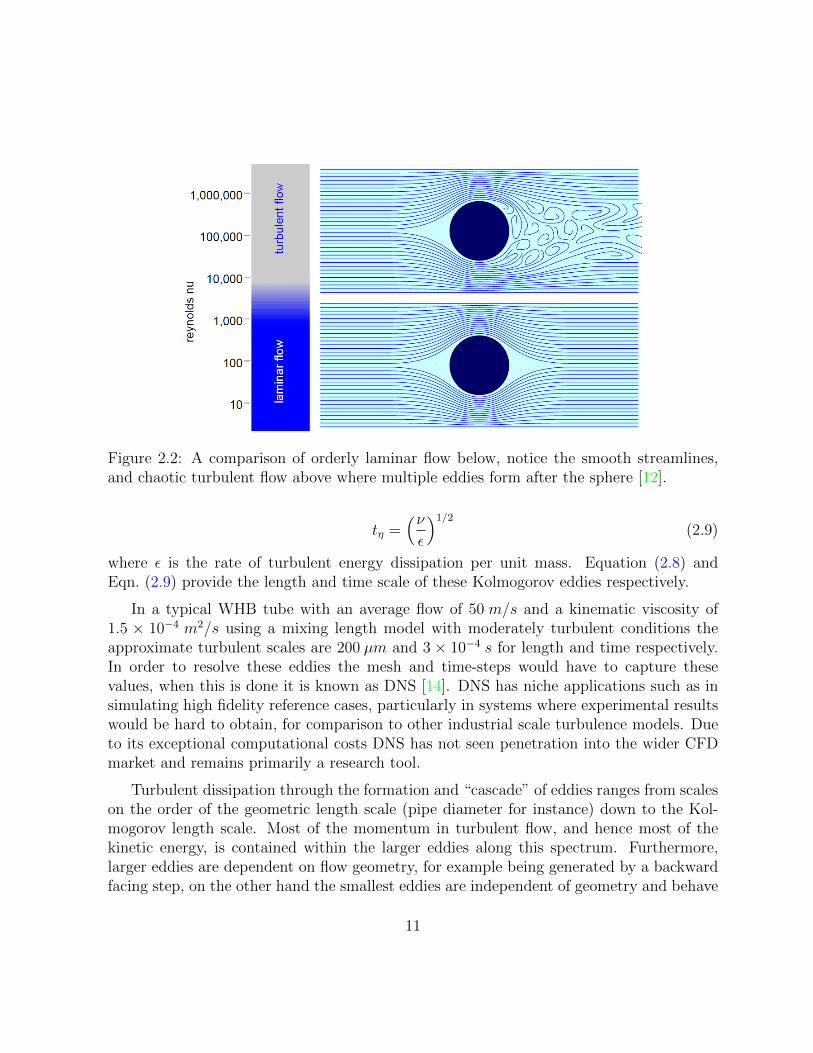


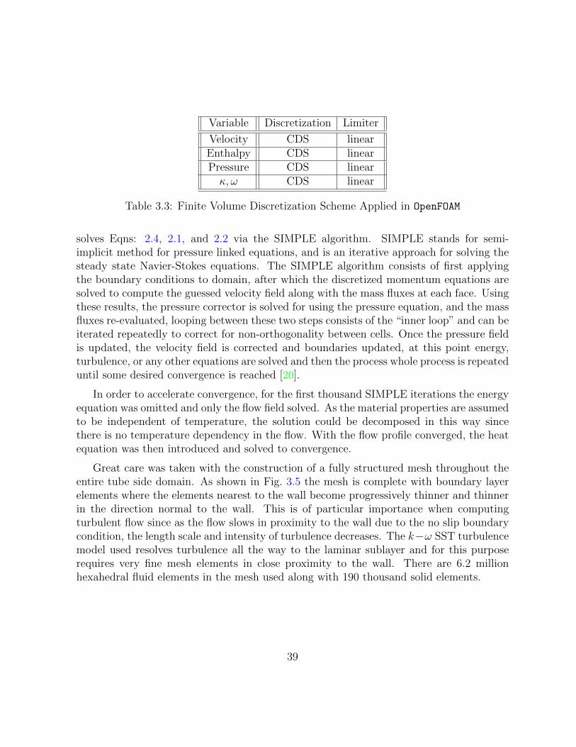


![Basic introduction of NWChem softwareinstitute.loni.org/NWChem2012/documents/2_NWChem_Intro.pdfNWChem: Gaussian DFT (2) Coupled Cluster Closed shell coupled cluster [CCSD and CCSD(T)]](https://static.documents.pub/doc/80x56/5e929a7b9e70f32e485c1392/basic-introduction-of-nwchem-nwchem-gaussian-dft-2-coupled-cluster-closed-shell.jpg)


