Under review as a conference paper at ICLR 2021

ITERATIVE GRAPH SELF-DISTILLATION

Anonymous authorsPaper under double-blind review

ABSTRACT

How to discriminatively vectorize graphs is a fundamental challenge that attractsincreasing attentions in recent years. Inspired by the recent success of unsupervisedcontrastive learning, we aim to learn graph-level representation in an unsupervisedmanner. Specifically, we propose a novel unsupervised graph learning paradigmcalled Iterative Graph Self-Distillation (IGSD) which iteratively performs theteacher-student distillation with graph augmentations. Different from conventionalknowledge distillation, IGSD constructs the teacher with an exponential movingaverage of the student model and distills the knowledge of itself. The intuitionbehind IGSD is to predict the teacher network representation of the graph pairsunder different augmented views. As a natural extension, we also apply IGSD tosemi-supervised scenarios by jointly regularizing the network with both supervisedand unsupervised contrastive loss. Finally, we show that finetuning the IGSD-trained models with self-training can further improve the graph representationpower. Empirically, we achieve significant and consistent performance gain onvarious graph datasets in both unsupervised and semi-supervised settings, whichwell validates the superiority of IGSD.

1 INTRODUCTION

Graphs are ubiquitous representations encoding relational structures across various domains. Learninglow-dimensional vector representations of graphs is critical in various domains ranging from socialscience (Newman & Girvan, 2004) to bioinformatics (Duvenaud et al., 2015; Zhou et al., 2020). Manygraph neural networks (GNNs) (Gilmer et al., 2017; Kipf & Welling, 2016; Xu et al., 2018) havebeen proposed to learn node and graph representations by aggregating information from every node’sneighbors via non-linear transformation and aggregation functions. However, the key limitation ofexisting GNN architectures is that they often require a huge amount of labeled data to be competitivebut annotating graphs like drug-target interaction networks is challenging since it needs domain-specific expertise. Therefore, unsupervised learning on graphs has been long studied, such as graphkernels (Shervashidze et al., 2011) and matrix-factorization approaches (Belkin & Niyogi, 2002).

Inspired by the recent success of unsupervised representation learning in various domains like images(Chen et al., 2020b; He et al., 2020) and texts (Radford et al., 2018), most related works in thegraph domain either follow the pipeline of unsupervised pretraining (followed by fine-tuning) orInfoMax principle (Hjelm et al., 2018). The former often needs meticulous designs of pretext tasks(Hu et al., 2019; You et al., 2020) while the latter is dominant in unsupervised graph representationlearning, which trains encoders to maximize the mutual information (MI) between the representationsof the global graph and local patches (such as subgraphs) (Velickovic et al., 2018; Sun et al., 2019;Hassani & Khasahmadi, 2020). However, MI-based approaches usually need to sample subgraphs aslocal views to contrast with global graphs. And they usually require an additional discriminator forscoring local-global pairs and negative samples, which is computationally prohibitive (Tschannenet al., 2019). Besides, the performance is also very sensitive to the choice of encoders and MIestimators (Tschannen et al., 2019). Moreover, MI-based approaches cannot be handily extendedto the semi-supervised setting since local subgraphs lack labels that can be utilized for training.Therefore, we are seeking an approach that learns the entire graph representation by contrasting thewhole graph directly without the need of MI estimation, discriminator and subgraph sampling.

Motivated by recent progress on contrastive learning, we propose the Iterative Graph Self-Distillation(IGSD), a teacher-student framework to learn graph representations by contrasting graph instancesdirectly. The high-level idea of IGSD is based on graph contrastive learning where we pull sim-

1

Under review as a conference paper at ICLR 2021

ilar graphs together and push dissimilar graph away. However, the performance of conventionalcontrastive learning largely depends on how negative samples are selected. To learn discriminativerepresentations and avoid collapsing to trivial solutions, a large set of negative samples (He et al.,2020; Chen et al., 2020b) or a special mining strategy (Schroff et al., 2015; He et al., 2020) arenecessary. In order to alleviate the dependency on negative samples mining and still be able to learndiscriminative graph representations, we propose to use self-distillation as a strong regularization toguide the graph representation learning.

In the IGSD framework, graph instances are augmented as several views to be encoded and projectedinto a latent space where we define a similarity metric for consistency-based training. The parametersof the teacher network are iteratively updated as an exponential moving average of the student networkparameters, allowing the knowledge transfer between them. As merely small amount of labeled datais often available in many real-world applications, we further extend IGSD to the semi-supervisedsetting such that it can effectively utilize graph-level labels while considering arbitrary amountsof positive pairs belonging to the same class. Moreover, in order to leverage the information frompseudo-labels with high confidence, we develop a self-training algorithm based on the supervisedcontrastive loss for fine-tuning.

We experiment with real-world datasets in various scales and compare the performance of IGSDwith state-of-the-art graph representation learning methods. Experimental results show that IGSDachieves competitive performance in both unsupervised and semi-supervised settings with differentencoders and data augmentation choices. With the help of self-training, our performance can exceedstate-of-the-art baselines by a large margin.

To summarize, we make the following contributions in this paper:

• We propose a self-distillation framework called IGSD for unsupervised graph-level representationlearning where the teacher-student distillation is performed for contrasting graph pairs underdifferent augmented views.

• We further extend IGSD to the semi-supervised scenario, where the labeled data are utilizedeffectively with the supervised contrastive loss and self-training.

• We empirically show that IGSD surpasses state-of-the-art methods in semi-supervised graphclassification and molecular property prediction tasks and achieves performance competitive withstate-of-the-art approaches in unsupervised graph classification tasks.

2 RELATED WORK

Contrastive Learning Modern unsupervised learning in the form of contrastive learning can becategorized into two types: context-instance contrast and context-context contrast (Liu et al., 2020).The context-instance contrast, or so-called global-local contrast focuses on modeling the belongingrelationship between the local feature of a sample and its global context representation. Mostunsupervised learning models on graphs like DGI (Velickovic et al., 2018), InfoGraph (Sun et al.,2019), CMC-Graph (Hassani & Khasahmadi, 2020) fall into this category, following the InfoMaxprinciple to maximize the the mutual information (MI) between the input and its representation.However, estimating MI is notoriously hard in MI-based contrastive learning and in practice tractablelower bound on this quantity is maximized instead. And maximizing tighter bounds on MI can resultin worse representations without stronger inductive biases in sampling strategies, encoder architectureand parametrization of MI estimators (Tschannen et al., 2019). Besides, the intricacies of negativesampling in MI-based approaches impose key research challenges like improper amount of negativesamples or biased negative sampling (Tschannen et al., 2019; Chuang et al., 2020). Another lineof contrastive learning approaches called context-context contrast directly study the relationshipsbetween the global representations of different samples as what metric learning does. For instance,a recently proposed model BYOL (Grill et al., 2020) bootstraps the representations of the wholeimages directly. Focusing on global representations between samples and corresponding augmentedviews also allows instance-level supervision to be incorporated naturally like introducing supervisedcontrastive loss (Khosla et al., 2020) into the framework for learning powerful representations.Graph Contrastive Coding (GCC) (Qiu et al., 2020) is a pioneer to leverage instance discriminationas the pretext task for structural information pre-training. However, our work is fundamentallydifferent from theirs. GCC focuses on structural similarity to find common and transferable structural

2

Under review as a conference paper at ICLR 2021

patterns across different graph datasets and the contrastive scheme is done through subgraph instancediscrimination. On the contrary, our model aims at learning graph-level representation by directlycontrasting graph instances such that data augmentation strategies and graph labels can be utilizednaturally and effectively.

Knowledge Distillation Knowledge distillation (Hinton et al., 2015) is a method for transferringknowledge from one architecture to another, allowing model compression and inductive biases transfer.Self-distillation (Furlanello et al., 2018) is a special case when two architectures are identical, whichcan iteratively modify regularization and reduce over-fitting if perform suitable rounds (Mobahi et al.,2020). However, they often focus on closing the gap between the predictive results of student andteacher rather than defining similarity loss in latent space for contrastive learning.

Semi-supervised Learning Modern semi-supervised learning can be categorized into two kinds:multi-task learning and consistency training between two separate networks. Most widely used semi-supervised learning methods take the form of multi-task learning: argminθ Ll(Dl, θ) +wLu(Du, θ)on labeled data Dl and unlabeled data Du. By regularizing the learning process with unlabeleddata, the decision boundary becomes more plausible. Another mainstream of semi-supervisedlearning lies in introducing student network and teacher network and enforcing consistency betweenthem (Tarvainen & Valpola, 2017; Miyato et al., 2019; Lee, 2013). It has been shown that semi-supervised learning performance can be greatly improved via unsupervised pre-training of a (big)model, supervised fine-tuning on a few labeled examples, and distillation with unlabeled examplesfor refining and transferring the task-specific knowledge (Chen et al., 2020c). However, whethertask-agnostic self-distillation would benefit semi-supervised learning is still underexplored.

3 PRELIMINARIES

3.1 FORMULATION

Unsupervised Graph Representation Learning Given a set of unlabeled graphs G = {Gi}Ni=1,we aim at learning the low-dimensional representation of every graph Gi ∈ G favorable for down-stream tasks like graph classification.

Semi-supervised Graph Representation Learning Consider a whole dataset G = GL ∪ GUcomposed by labeled data GL = {(Gi, yi)}li=1 and unlabeled data GU = {Gi}l+ui=l+1 (usually u� l),our goal is to learn a model that can make predictions on graph labels for unseen graphs. And with Kaugmentations, we get G′L = {(G′k, y′k)}Klk=1 and G′U = {G′k}

K(l+u)k=l+1 as our training data.

3.2 GRAPH REPRESENTATION LEARNING

We represent a graph instance as G(V, E) with the node set V and the edge set E . The dominant waysof graph representation learning are graph neural networks with neural message passing mechanisms(Hamilton et al., 2017): for every node v ∈ V , node representation hkv is iteratively computed fromthe features of their neighbor nodes N (v) using a differentiable aggregation function. Specifically, atthe iteration k we get the node embedding as:

hkv = σ(Wk · CONCAT

(hk−1v ,AGGREGATEk

({hk−1u ,∀u ∈ N (v)

})))(1)

Then the graph-level representations can be attained by aggregating all node representations using areadout function like summation or set2set pooling (Vinyals et al., 2015).

3.3 GRAPH DATA AUGMENTATION

It has been shown that the learning performance of GNNs can be improved via graph diffusion, whichserves as a homophily-based denoising filter on both features and edges in real graphs (Klicpera et al.,2019). The transformed graphs can also serve as effective augmented views in contrastive learning(Hassani & Khasahmadi, 2020). Inspired by that, we transform a graph G with transition matrixT via graph diffusion and sparsification S =

∑∞k=0 θkT

k into a new graph with adjacency matrixS as an augmented view in our framework. While there are many design choices in coefficientsθk like heat kernel, we employ Personalized PageRank (PPR) with θPPRk = α(1 − α)k due to its

3

Under review as a conference paper at ICLR 2021

superior empirical performance (Hassani & Khasahmadi, 2020). As another augmentation choice,we randomly remove edges of graphs to attain corrupted graphs as augmented views to validate therobustness of models to different augmentation choices.

4 ITERATIVE GRAPH SELF-DISTILLATION

Intuitively, the goal of contrastive learning on graphs is to learn graph representations that are closein the metric space for positive pairs (graphs with the same labels) and far between negative pairs(graphs with different labels). To achieve this goal, IGSD employs the teacher-student distillation toiteratively refine representations by contrasting latent representations embedded by two networks andusing additional predictor and EMA update to avoid collapsing to trivial solutions. Overall, IGSDencourages the closeness of augmented views from the same graph instances while pushing apart therepresentations from different ones.

4.1 ITERATIVE GRAPH SELF-DISTILLATION FRAMEWORK

Encoder ProjectorPredictor

𝐺!𝐺!′

𝐺"𝐺"′

𝐺#𝐺#′

Augmentation Latent Contrast

EMAUpdate

𝑓! 𝑔! ℎ!

𝑓!!

𝐺!

𝐺"

𝐺#

Mini-Batch

𝑔!!

𝑧!′

𝑧"′

𝑧#′

ℎ!(𝑧")

ℎ!(𝑧#)

ℎ!(𝑧$)

Figure 1: Overview of IGSD. Illustration of ourframework in the case where we augment inputgraphs G once to get G′ for only one forwardpass. Blue and red arrows denote contrast onpositive and negative pairs respectively.

In IGSD, we introduce a teacher-student architec-ture comprises two networks in similar structurecomposed by encoder fθ, projector gθ and predic-tor hθ. We denote the components of the teachernetwork and the student network as fθ′ , gθ′ andfθ, gθ, hθ respectively.

The overview of IGSD is illustrated in Figure1. In IGSD, the procedure of contrastive learn-ing on negative pairs is described as follows: wefirst augment the original input graphs Gj to getaugmented view(s) G′j . Then G′j and differentgraph instance Gi are fed respectively into twoencoders fθ, fθ′ for extracting graph represen-tations h,h′ = fθ(Gi), fθ′(G

′j) with iterative

message passing in Eqn. (1) and readout func-tions. The following projectors gθ, gθ′ transformgraph representations to projections z, z′ via z = gθ(h) = W (2)σ(W (1)h) and z′ = gθ′(h

′) =W ′(2)σ(W ′(1)h′), where σ denotes a ReLU nonlinearity1. To prevent collapsing into a trivial solution(Grill et al., 2020), a specialized predictor is used in the student network for attaining the predictionhθ(z) =W

(2)h σ(W

(1)h z) of the projection z. For positive pairs, we follow the same procedure except

feeding the original and augmented view of the same graph into two networks respectively.

To contrast latents hθ(z) and z′, we use L2 norm in the latent space to approximate the semanticdistance in the input space and the consistency loss can be defined as the mean square error betweenthe normalized prediction hθ(z) and projection z′. By passing two graph instances Gi and Gjsymmetrically, we can obtain the overall consistency loss:

Lcon(Gi, Gj) =∥∥hθ (zi)− z′j

∥∥22+ ‖hθ (z′i)− zj‖

2

2 (2)

With the consistency loss, the teacher network provides a regression target to train the student network,and its parameters θ′ are updated as an exponential moving average (EMA) of the student parametersθ after weights of the student network have been updated using gradient descent:

θ′t ← τθ′t−1 + (1− τ)θt (3)

With the above iterative self-distillation procedure, we can aggregate information for averagingmodel weights over each training step instead of using the final weights directly (Athiwaratkun et al.,2018). It should be noted that maintaining a slow-moving average network is also employed in somemodels like MoCo (He et al., 2020) with different motivations: MoCo uses an EMA of encoder

1Although IGSD could directly predict the representations without projections, previous contrastive learningwork (Chen et al., 2020b) in the image domain has shown that using projections improves performanceempirically. We include the experimental results to validate the effects of projectors in Appendix A.3

4

Under review as a conference paper at ICLR 2021

and momentum encoder to update the encoder, ensuring the consistency of dictionary keys in thememory bank. On the other hand, IGSD uses a moving average network to produce prediction targets,enforcing the consistency of teacher and student for training the student network.

4.2 UNSUPERVISED LEARNING WITH IGSD

In IGSD, to contrast the anchor Gi with other graph instances Gj (i.e. negative samples), we employthe following unsupervised InfoNCE objective (Oord et al., 2018):

Lunsup = −EGi∼G

[log

exp (−Lcon(Gi, Gi))

exp (−Lcon(Gi, Gi)) +∑N−1j=1 Ii6=j · exp (−Lcon(Gi, Gj))

](4)

At the inference time, as semantic interpolations on samples, labels and latents result in betterrepresentations and can improve learning performance greatly (Zhang et al., 2017; Verma et al., 2019;Berthelot et al., 2019), we obtain the graph representation h by interpolating the latent representationsh = fθ(G) and h′ = fθ′(G) with Mixup function Mixλ(a, b) = λ · a+ (1− λ) · b:

h = Mixλ(h,h′) (5)

4.3 SEMI-SUPERVISED LEARNING WITH IGSD

To bridge the gap between unsupervised pretraining and downstream tasks, we extend our model tothe semi-supervised setting. In this scenario, it is straightforward to plug in the unsupervised loss as aregularizer for representation learning. However, the instance-wise supervision limited to standardsupervised learning may lead to biased negative sampling problems (Chuang et al., 2020). To tacklethis challenge, we can use a small amount of labeled data further to generalize the similarity loss tohandle arbitrary number of positive samples belonging to the same class:

Lsupcon =

Kl∑i=1

1

KNy′i

Kl∑j=1

Ii6=j · Iy′i=y′j · Lcon(Gi, Gj) (6)

where Ny′i denotes the total number of samples in the training set that have the same label y′i asanchor i. Thanks to the graph-level contrastive nature of IGSD, we are able to alleviate the biasednegative sampling problems (Khosla et al., 2020) with supervised contrastive loss, which is crucial(Chuang et al., 2020) but unachievable in most MI-based contrastive learning models since subgraphsare generally hard to assign labels to. Besides, with this loss we are able to fine-tune our modeleffectively using self-training where pseudo-labels are assigned iteratively to unlabeled data.

With the standard supervised loss like cross entropy or mean square error L(GL, θ), the overallobjective can be summarized as:

Lsemi = L(GL, θ) + wLunsup(GL ∪ GU , θ) + w′Lsupcon(GL, θ) (7)

Common semi-supervised learning methods use consistency regularization to measure discrepancybetween predictions made on perturbed unlabeled data points for better prediction stability andgeneralization (Oliver et al., 2018). By contrast, our methods enforce consistency constraints betweenlatents from different views, which acts as a regularizer for learning directly from labels.

Labeled data provides extra supervision about graph classes and alleviates biased negative sampling.However, they are costly to attain in many areas. Therefore, we develop a contrastive self-trainingalgorithm to leverage label information more effectively than cross entropy in the semi-supervisedscenario. In the algorithm, we train the model using a small amount of labeled data and then fine-tuneit by iterating between assigning pseudo-labels to unlabeled examples and training models using theaugmented dataset. In this way, we harvest massive pseudo-labels for unlabeled examples.

With increasing size of the augmented labeled dataset, the discriminative power of IGSD can beimproved iteratively by contrasting more positive pairs belonging to the same class. In this way, weaccumulate high-quality psuedo-labels after each iteration to compute the supervised contrastive lossin Eqn. (6) and make distinction from conventional self-training algorithms (Rosenberg et al., 2005).On the other hand, traditional self-training can use psuedo-labels for computing cross entropy only.

5

Under review as a conference paper at ICLR 2021

5 EXPERIMENTS

5.1 EXPERIMENTAL SETUP

Evaluation Tasks. We conduct experiments by comparing with state-of-the-art models on threetasks. In graph classification tasks, we experiment in both the unsupervised setting where we onlyhave access to all unlabeled samples in the dataset and the semi-supervised setting where we use asmall fraction of labeled examples and treat the rest as unlabeled ones by ignoring their labels. Inmolecular property prediction tasks where labels are expensive to obtain, we only consider thesemi-supervised setting.

Datasets. For graph classification tasks, we employ several widely-used graph kernel datasets(Kersting et al., 2016) for learning and evaluation: 3 bioinformatics datasets (MUTAG, PTC, NCI1)and 3 social network datasets (COLLAB, IMDB-B, IMDB-M) with statistics summarized in Table1. In the semi-supervised graph regression tasks, we use the QM9 dataset containing 134,000drug-like organic molecules (Ramakrishnan et al., 2014) with 9 heavy atoms and select the first tenphysicochemical properties as regression targets for training and evaluation. For detailed descriptionof the properties in the QM9 dataset, see the Appendix C of (Sun et al., 2019).

Baselines. In the unsupervised graph classification, we compare with the following representativebaselines: CMC-Graph (Hassani & Khasahmadi, 2020), InfoGraph (Sun et al., 2019), GCC (Qiuet al., 2020), Graph2Vec (Narayanan et al., 2017) and Graph Kernels including Random Walk Kernel(Gartner et al., 2003), Shortest Path Kernel (Kashima et al., 2003), Graphlet Kernel (Shervashidzeet al., 2009), Weisfeiler-Lehman Sub-tree Kernel (WL SubTree) (Shervashidze et al., 2011), DeepGraph Kernels (Yanardag & Vishwanathan, 2015), Multi-Scale Laplacian Kernel (MLG) (Kondor &Pan, 2016) and Graph Convolutional Kernel Network (GCKN) (Chen et al., 2020a).

For the semi-supervised graph classification, we compare our method with competitive baselineslike InfoGraph, InfoGraph* and Mean Teachers. And the GIN baseline doesn’t have access tothe unlabeled data. In the semi-supervised molecular property prediction tasks, baselines includeInfoGraph, InfoGraph* and Mean Teachers (Tarvainen & Valpola, 2017).

Model Configuration. In our framework, We use GCNs (Kipf & Welling, 2016) and GINs (Xuet al., 2018) as encoders to attain node representations for unsupervised and semi-supervised graphclassification respectively. For semi-supervised molecular property prediction, we employ messagepassing neural networks (MPNNs) (Gilmer et al., 2017) as backbone encoders to encode moleculargraphs with rich edge attributes. All projectors and predictors are implemented as two-layer MLPs.For more details on hyper-parameters selection, refer to appendix A.2

In semi-supervised molecular property prediction tasks, we generate multiple views based on edgeattributes (bond types) of rich-annotated molecular graphs for improving performance. Specifically,we perform label-preserving augmentation to attain multiple diffusion matrixes of every graph ondifferent edge attributes while ignoring others respectively. The diffusion matrix gives a denser graphbased on each type of edges to leverage edge features better. We train our models using differentnumbers of augmented training data and select the amount using cross validation.

For unsupervised graph classification, we adopt LIB-SVM (Chang & Lin, 2011) with C parameterselected in {1e-3, 1e-2, . . . , 1e2, 1e3} as our downstream classifier. Then we use 10-fold crossvalidation accuracy as the classification performance and repeat the experiments 5 times to report themean and standard deviation. For semi-supervised graph classification, we randomly select 5% oftraining data as labeled data while treat the rest as unlabeled one and report the best test set accuracyin 300 epochs. Following the experimental setup in (Sun et al., 2019), we randomly choose 5000,10000, 10000 samples for training, validation and testing respectively and the rest are treated asunlabeled training data for the molecular property prediction tasks.

5.2 NUMERICAL RESULTS

Results on unsupervised graph classification. We first present the results of the unsupervisedsetting in Table 1. All graph kernels give inferior performance except in the PTC dataset. TheRandom Walk kernel runs out of memory and the Multi-Scale Laplacian Kernel suffers from a longrunning time (exceeds 24 hours) in two larger datasets. IGSD outperforms state-of-the-art baselines

6

Under review as a conference paper at ICLR 2021

Datasets MUTAG IMDB-B IMDB-M NCI1 COLLAB PTC

Dat

aset

s # graphs 188 1000 1500 4110 5000 344# classes 2 2 3 2 3 2Avg # nodes 17.9 19.8 13.0 29.8 74.5 25.5

Gra

phK

erne

ls

Random Walk 83.7± 1.5 50.7± 0.3 34.7± 0.2 OMR OMR 57.9± 1.3SHORTEST PATH 85.2± 2.4 55.6± 0.2 38.0± 0.3 51.3± 0.6 49.8± 1.2 58.2± 2.4GRAPHLET KERNEL 81.7± 2.1 65.9± 1.0 43.9± 0.4 53.9± 0.4 56.3± 0.6 57.3± 1.4WL SUBTREE 80.7± 3.0 72.3± 3.4 47.0± 0.5 55.1± 1.6 50.2± 0.9 58.0± 0.5DEEP GRAPH 87.4± 2.7 67.0± 0.6 44.6± 0.5 54.5± 1.2 52.1± 1.0 60.1± 2.6MLG 87.9± 1.6 66.6± 0.3 41.2± 0.0 >1 Day >1 Day 63.3± 1.5GCKN 87.2± 6.8 70.5± 3.1 50.8± 0.8 70.6± 2.0 54.3±1.0 58.4± 7.6

Uns

uper

vise

d

GRAPH2VEC 83.2± 9.6 71.1± 0.5 50.4± 0.9 73.2± 1.8 47.9± 0.3 60.2± 6.9INFOGRAPH 89.0± 1.1 74.2± 0.7 49.7± 0.5 73.8± 0.7 67.6± 1.2 61.7±1.7CMC-GRAPH 89.7± 1.1 74.2± 0.7 51.2± 0.5 75.0± 0.7 68.9± 1.9 62.5± 1.7GCC 86.4± 0.5 71.9± 0.5 48.9± 0.8 66.9± 0.2 75.2± 0.3 58.4± 1.2OURS (RANDOM) 85.7± 2.1 71.6± 1.2 49.2± 0.6 75.1± 0.4 65.8± 1.0 57.6± 1.5OURS 90.2± 0.7 74.7± 0.6 51.5± 0.3 75.4± 0.3 70.4± 1.1 61.4± 1.7

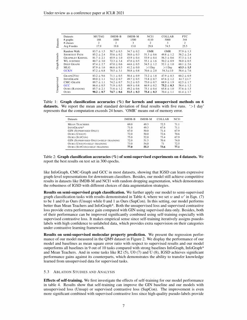
Table 1: Graph classification accuracies (%) for kernels and unsupervised methods on 6datasets. We report the mean and standard deviation of final results with five runs. ‘>1 day’represents that the computation exceeds 24 hours. ‘OMR’ means out of memory error.

Datasets IMDB-B IMDB-M COLLAB NCI1

MEAN TEACHERS 69.0 49.3 72.5 71.1INFOGRAPH* 71.0 49.3 67.6 71.1GIN (SUPERVISED ONLY) 67.0 50.0 71.4 67.9OURS (UNSUP) 72.0 50.0 72.6 70.6OURS (SUPCON) 75.0 52.0 73.4 67.9GIN (SUPERVISED ONLY)+SELF-TRAINING 72.0 51.3 70.4 74.0OURS (UNSUP)+SELF-TRAINING 73.0 54,0 71 72.5OURS (SUPCON)+SELF-TRAINING 77.0 55.3 73.6 77.1

Table 2: Graph classification accuracies (%) of semi-supervised experiments on 4 datasets. Wereport the best results on test set in 300 epochs.

like InfoGraph, CMC-Graph and GCC in most datasets, showing that IGSD can learn expressivegraph-level representations for downstream classifiers. Besides, our model still achieve competitiveresults in datasets like IMDB-M and NCI1 with random dropping augmentation, which demonstratesthe robustness of IGSD with different choices of data augmentation strategies.

Results on semi-supervised graph classification. We further apply our model to semi-supervisedgraph classification tasks with results demonstrated in Table 4, where we set w and w′ in Eqn. (7)to be 1 and 0 as Ours (Unsup) while 0 and 1 as Ours (SupCon). In this setting, our model performsbetter than Mean Teachers and InfoGraph*. Both the unsupervised loss and supervised contrastiveloss provide extra performance gain compared with GIN using supervised data only. Besides, bothof their performance can be improved significantly combined using self-training especially withsupervised contrastive loss. It makes empirical sense since self-training iteratively assigns psuedo-labels with high confidence to unlabeled data, which provides extra supervision on their categoriesunder contrastive learning framework.

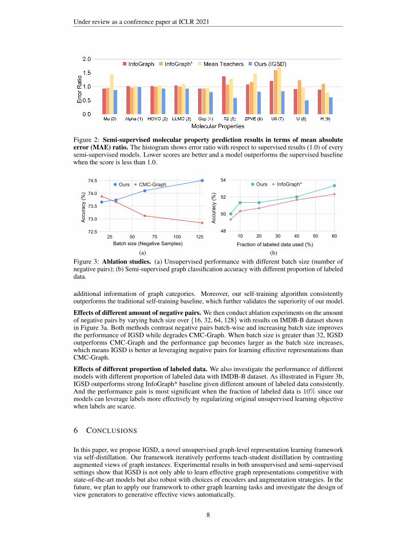
Results on semi-supervised molecular property prediction. We present the regression perfor-mance of our model measured in the QM9 dataset in Figure 2. We display the performance of ourmodel and baselines as mean square error ratio with respect to supervised results and our modeloutperforms all baselines in 9 out of 10 tasks compared with strong baselines InfoGraph, InfoGraph*and Mean Teachers. And in some tasks like R2 (5), U0 (7) and U (8), IGSD achieves significantperformance gains against its counterparts, which demonstrates the ability to transfer knowledgelearned from unsupervised data for supervised tasks.

5.3 ABLATION STUDIES AND ANALYSIS

Effects of self-training. We first investigate the effects of self-training for our model performancein table 4. Results show that self-training can improve the GIN baseline and our models withunsupervised loss (Unsup) or supervised contrastive loss (SupCon). The improvement is evenmore significant combined with supervised contrastive loss since high-quality pseudo-labels provide

7

Under review as a conference paper at ICLR 2021

Figure 2: Semi-supervised molecular property prediction results in terms of mean absoluteerror (MAE) ratio. The histogram shows error ratio with respect to supervised results (1.0) of everysemi-supervised models. Lower scores are better and a model outperforms the supervised baselinewhen the score is less than 1.0.

%DWFK�VL]H��1HJDWLYH�6DPSOHV�

$FFXUDF\����

����

����

����

����

����

�� �� �� ��� ���

2XUV &0&�*UDSK

(a))UDFWLRQ�RI�ODEHOHG�GDWD�XVHG����

$FFXUDF\����

��

��

��

��

�� �� �� �� �� ��

2XUV ,QIR*UDSK

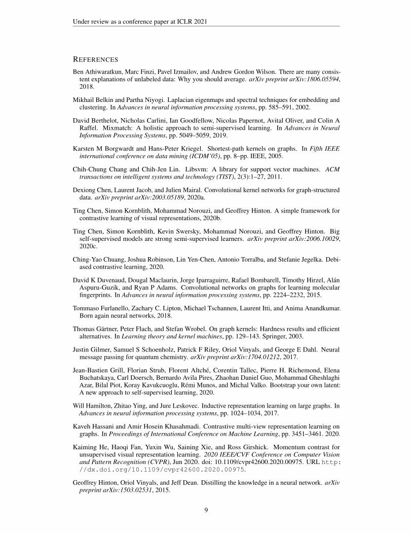
(b)Figure 3: Ablation studies. (a) Unsupervised performance with different batch size (number ofnegative pairs); (b) Semi-supervised graph classification accuracy with different proportion of labeleddata.

additional information of graph categories. Moreover, our self-training algorithm consistentlyoutperforms the traditional self-training baseline, which further validates the superiority of our model.

Effects of different amount of negative pairs. We then conduct ablation experiments on the amountof negative pairs by varying batch size over {16, 32, 64, 128} with results on IMDB-B dataset shownin Figure 3a. Both methods contrast negative pairs batch-wise and increasing batch size improvesthe performance of IGSD while degrades CMC-Graph. When batch size is greater than 32, IGSDoutperforms CMC-Graph and the performance gap becomes larger as the batch size increases,which means IGSD is better at leveraging negative pairs for learning effective representations thanCMC-Graph.

Effects of different proportion of labeled data. We also investigate the performance of differentmodels with different proportion of labeled data with IMDB-B dataset. As illustrated in Figure 3b,IGSD outperforms strong InfoGraph* baseline given different amount of labeled data consistently.And the performance gain is most significant when the fraction of labeled data is 10% since ourmodels can leverage labels more effectively by regularizing original unsupervised learning objectivewhen labels are scarce.

6 CONCLUSIONS

In this paper, we propose IGSD, a novel unsupervised graph-level representation learning frameworkvia self-distillation. Our framework iteratively performs teach-student distillation by contrastingaugmented views of graph instances. Experimental results in both unsupervised and semi-supervisedsettings show that IGSD is not only able to learn effective graph representations competitive withstate-of-the-art models but also robust with choices of encoders and augmentation strategies. In thefuture, we plan to apply our framework to other graph learning tasks and investigate the design ofview generators to generative effective views automatically.

8

Under review as a conference paper at ICLR 2021

REFERENCES

Ben Athiwaratkun, Marc Finzi, Pavel Izmailov, and Andrew Gordon Wilson. There are many consis-tent explanations of unlabeled data: Why you should average. arXiv preprint arXiv:1806.05594,2018.

Mikhail Belkin and Partha Niyogi. Laplacian eigenmaps and spectral techniques for embedding andclustering. In Advances in neural information processing systems, pp. 585–591, 2002.

David Berthelot, Nicholas Carlini, Ian Goodfellow, Nicolas Papernot, Avital Oliver, and Colin ARaffel. Mixmatch: A holistic approach to semi-supervised learning. In Advances in NeuralInformation Processing Systems, pp. 5049–5059, 2019.

Karsten M Borgwardt and Hans-Peter Kriegel. Shortest-path kernels on graphs. In Fifth IEEEinternational conference on data mining (ICDM’05), pp. 8–pp. IEEE, 2005.

Chih-Chung Chang and Chih-Jen Lin. Libsvm: A library for support vector machines. ACMtransactions on intelligent systems and technology (TIST), 2(3):1–27, 2011.

Dexiong Chen, Laurent Jacob, and Julien Mairal. Convolutional kernel networks for graph-structureddata. arXiv preprint arXiv:2003.05189, 2020a.

Ting Chen, Simon Kornblith, Mohammad Norouzi, and Geoffrey Hinton. A simple framework forcontrastive learning of visual representations, 2020b.

Ting Chen, Simon Kornblith, Kevin Swersky, Mohammad Norouzi, and Geoffrey Hinton. Bigself-supervised models are strong semi-supervised learners. arXiv preprint arXiv:2006.10029,2020c.

Ching-Yao Chuang, Joshua Robinson, Lin Yen-Chen, Antonio Torralba, and Stefanie Jegelka. Debi-ased contrastive learning, 2020.

David K Duvenaud, Dougal Maclaurin, Jorge Iparraguirre, Rafael Bombarell, Timothy Hirzel, AlanAspuru-Guzik, and Ryan P Adams. Convolutional networks on graphs for learning molecularfingerprints. In Advances in neural information processing systems, pp. 2224–2232, 2015.

Tommaso Furlanello, Zachary C. Lipton, Michael Tschannen, Laurent Itti, and Anima Anandkumar.Born again neural networks, 2018.

Thomas Gartner, Peter Flach, and Stefan Wrobel. On graph kernels: Hardness results and efficientalternatives. In Learning theory and kernel machines, pp. 129–143. Springer, 2003.

Justin Gilmer, Samuel S Schoenholz, Patrick F Riley, Oriol Vinyals, and George E Dahl. Neuralmessage passing for quantum chemistry. arXiv preprint arXiv:1704.01212, 2017.

Jean-Bastien Grill, Florian Strub, Florent Altche, Corentin Tallec, Pierre H. Richemond, ElenaBuchatskaya, Carl Doersch, Bernardo Avila Pires, Zhaohan Daniel Guo, Mohammad GheshlaghiAzar, Bilal Piot, Koray Kavukcuoglu, Remi Munos, and Michal Valko. Bootstrap your own latent:A new approach to self-supervised learning, 2020.

Will Hamilton, Zhitao Ying, and Jure Leskovec. Inductive representation learning on large graphs. InAdvances in neural information processing systems, pp. 1024–1034, 2017.

Kaveh Hassani and Amir Hosein Khasahmadi. Contrastive multi-view representation learning ongraphs. In Proceedings of International Conference on Machine Learning, pp. 3451–3461. 2020.

Kaiming He, Haoqi Fan, Yuxin Wu, Saining Xie, and Ross Girshick. Momentum contrast forunsupervised visual representation learning. 2020 IEEE/CVF Conference on Computer Visionand Pattern Recognition (CVPR), Jun 2020. doi: 10.1109/cvpr42600.2020.00975. URL http://dx.doi.org/10.1109/cvpr42600.2020.00975.

Geoffrey Hinton, Oriol Vinyals, and Jeff Dean. Distilling the knowledge in a neural network. arXivpreprint arXiv:1503.02531, 2015.

9

Under review as a conference paper at ICLR 2021

R Devon Hjelm, Alex Fedorov, Samuel Lavoie-Marchildon, Karan Grewal, Phil Bachman, AdamTrischler, and Yoshua Bengio. Learning deep representations by mutual information estimationand maximization. arXiv preprint arXiv:1808.06670, 2018.

Weihua Hu, Bowen Liu, Joseph Gomes, Marinka Zitnik, Percy Liang, Vijay Pande, and Jure Leskovec.Strategies for pre-training graph neural networks, 2019.

Hisashi Kashima, Koji Tsuda, and Akihiro Inokuchi. Marginalized kernels between labeled graphs.In Proceedings of the 20th international conference on machine learning (ICML-03), pp. 321–328,2003.

Kristian Kersting, Nils M. Kriege, Christopher Morris, Petra Mutzel, and Marion Neumann. Bench-mark data sets for graph kernels, 2016. URL http://graphkernels.cs.tu-dortmund.de.

Prannay Khosla, Piotr Teterwak, Chen Wang, Aaron Sarna, Yonglong Tian, Phillip Isola, AaronMaschinot, Ce Liu, and Dilip Krishnan. Supervised contrastive learning, 2020.

Thomas N Kipf and Max Welling. Semi-supervised classification with graph convolutional networks.arXiv preprint arXiv:1609.02907, 2016.

Johannes Klicpera, Stefan Weißenberger, and Stephan Gunnemann. Diffusion improves graphlearning, 2019.

Risi Kondor and Horace Pan. The multiscale laplacian graph kernel. In Advances in NeuralInformation Processing Systems, pp. 2990–2998, 2016.

Dong-Hyun Lee. Pseudo-label: The simple and efficient semi-supervised learning method for deepneural networks. In Workshop on challenges in representation learning, ICML, volume 3, 2013.

Xiao Liu, Fanjin Zhang, Zhenyu Hou, Zhaoyu Wang, Li Mian, Jing Zhang, and Jie Tang. Self-supervised learning: Generative or contrastive, 2020.

Takeru Miyato, Shin-Ichi Maeda, Masanori Koyama, and Shin Ishii. Virtual adversarial training: Aregularization method for supervised and semi-supervised learning. IEEE Transactions on PatternAnalysis and Machine Intelligence, 41(8):1979–1993, Aug 2019. ISSN 1939-3539. doi: 10.1109/tpami.2018.2858821. URL http://dx.doi.org/10.1109/TPAMI.2018.2858821.

Hossein Mobahi, Mehrdad Farajtabar, and Peter L Bartlett. Self-distillation amplifies regularizationin hilbert space. arXiv preprint arXiv:2002.05715, 2020.

Annamalai Narayanan, Mahinthan Chandramohan, Rajasekar Venkatesan, Lihui Chen, Yang Liu,and Shantanu Jaiswal. graph2vec: Learning distributed representations of graphs. arXiv preprintarXiv:1707.05005, 2017.

Mark EJ Newman and Michelle Girvan. Finding and evaluating community structure in networks.Physical review E, 69(2):026113, 2004.

Avital Oliver, Augustus Odena, Colin Raffel, Ekin D. Cubuk, and Ian J. Goodfellow. Realisticevaluation of deep semi-supervised learning algorithms, 2018.

Aaron van den Oord, Yazhe Li, and Oriol Vinyals. Representation learning with contrastive predictivecoding. arXiv preprint arXiv:1807.03748, 2018.

Jiezhong Qiu, Qibin Chen, Yuxiao Dong, Jing Zhang, Hongxia Yang, Ming Ding, Kuansan Wang,and Jie Tang. Gcc: Graph contrastive coding for graph neural network pre-training. In Proceedingsof the 26th ACM SIGKDD International Conference on Knowledge Discovery & Data Mining, pp.1150–1160, 2020.

Alec Radford, Karthik Narasimhan, Tim Salimans, and Ilya Sutskever. Improving language under-standing by generative pre-training, 2018.

Raghunathan Ramakrishnan, Pavlo O Dral, Matthias Rupp, and O Anatole Von Lilienfeld. Quantumchemistry structures and properties of 134 kilo molecules. Scientific data, 1(1):1–7, 2014.

10

Under review as a conference paper at ICLR 2021

Chuck Rosenberg, Martial Hebert, and Henry Schneiderman. Semi-supervised self-training of objectdetection models. 2005.

Florian Schroff, Dmitry Kalenichenko, and James Philbin. Facenet: A unified embedding for facerecognition and clustering. In Proceedings of the IEEE conference on computer vision and patternrecognition, pp. 815–823, 2015.

Nino Shervashidze, SVN Vishwanathan, Tobias Petri, Kurt Mehlhorn, and Karsten Borgwardt.Efficient graphlet kernels for large graph comparison. In Artificial Intelligence and Statistics, pp.488–495, 2009.

Nino Shervashidze, Pascal Schweitzer, Erik Jan Van Leeuwen, Kurt Mehlhorn, and Karsten MBorgwardt. Weisfeiler-lehman graph kernels. Journal of Machine Learning Research, 12(9), 2011.

Fan-Yun Sun, Jordan Hoffmann, Vikas Verma, and Jian Tang. Infograph: Unsupervised and semi-supervised graph-level representation learning via mutual information maximization. arXiv preprintarXiv:1908.01000, 2019.

Antti Tarvainen and Harri Valpola. Mean teachers are better role models: Weight-averaged consistencytargets improve semi-supervised deep learning results, 2017.

Yonglong Tian, Chen Sun, Ben Poole, Dilip Krishnan, Cordelia Schmid, and Phillip Isola. Whatmakes for good views for contrastive learning? arXiv preprint arXiv:2005.10243, 2020.

Michael Tschannen, Josip Djolonga, Paul K Rubenstein, Sylvain Gelly, and Mario Lucic. On mutualinformation maximization for representation learning. arXiv preprint arXiv:1907.13625, 2019.

Petar Velickovic, William Fedus, William L Hamilton, Pietro Lio, Yoshua Bengio, and R DevonHjelm. Deep graph infomax. arXiv preprint arXiv:1809.10341, 2018.

Vikas Verma, Alex Lamb, Christopher Beckham, Amir Najafi, Ioannis Mitliagkas, David Lopez-Paz,and Yoshua Bengio. Manifold mixup: Better representations by interpolating hidden states. InInternational Conference on Machine Learning, pp. 6438–6447. PMLR, 2019.

Oriol Vinyals, Samy Bengio, and Manjunath Kudlur. Order matters: Sequence to sequence for sets,2015.

Keyulu Xu, Weihua Hu, Jure Leskovec, and Stefanie Jegelka. How powerful are graph neuralnetworks? arXiv preprint arXiv:1810.00826, 2018.

Pinar Yanardag and SVN Vishwanathan. Deep graph kernels. In Proceedings of the 21th ACMSIGKDD International Conference on Knowledge Discovery and Data Mining, pp. 1365–1374,2015.

Yuning You, Tianlong Chen, Zhangyang Wang, and Yang Shen. When does self-supervision helpgraph convolutional networks? arXiv preprint arXiv:2006.09136, 2020.

Hongyi Zhang, Moustapha Cisse, Yann N. Dauphin, and David Lopez-Paz. mixup: Beyond empiricalrisk minimization, 2017.

Tong Zhao, Yozen Liu, Leonardo Neves, Oliver Woodford, Meng Jiang, and Neil Shah. Dataaugmentation for graph neural networks, 2020.

Yadi Zhou, Fei Wang, Jian Tang, Ruth Nussinov, and Feixiong Cheng. Artificial intelligence incovid-19 drug repurposing. The Lancet Digital Health, 2020.

11

Under review as a conference paper at ICLR 2021

A APPENDIX

A.1 RELATED WORK

Graph Representation Learning Traditionally, graph kernels are widely used for learning nodeand graph representations. This common process includes meticulous designs like decomposinggraphs into substructures and using kernel functions like Weisfeiler-Leman graph kernel (Shervashidzeet al., 2011) to measure graph similarity between them. However, they usually require non-trivialhand-crafted substructures and domain-specific kernel functions to measure the similarity while yieldsinferior performance on downstream tasks like node classification and graph classification. Moreover,they often suffer from poor scalability (Borgwardt & Kriegel, 2005) and great memory consumption(Kondor & Pan, 2016) due to some procedures like path extraction and recursive subgraph construction.Recently, there has been increasing interest in Graph Neural Network (GNN) approaches for graphrepresentation learning and many GNN variants have been proposed (Ramakrishnan et al., 2014; Kipf& Welling, 2016; Xu et al., 2018). However, they mainly focus on supervised settings.

Data augmentation Data augmentation strategies on graphs are limited since defining views ofgraphs is a non-trivial task. There are two common choices of augmentations on graphs (1) feature-space augmentation and (2) structure-space augmentation. A straightforward way is to corruptthe adjacency matrix which preserves the features but adds or removes edges from the adjacencymatrix with some probability distribution (Velickovic et al., 2018). Zhao et al. (2020) improvesperformance in GNN-based semi-supervised node classification via edge prediction. Empirical resultsshow that diffusion matrix can serve as a denoising filter to augment graph data for improving graphrepresentation learning significantly both in supervised (Klicpera et al., 2019) and unsupervisedsettings (Hassani & Khasahmadi, 2020). Hassani & Khasahmadi (2020) shows the benefits of treatingdiffusion matrix as an augmented view of mutual information-based contrastive graph representationlearning. Attaining effective views is non-trivial since we need to consider factors like mutualinformation to preserve label information w.r.t the downstream task (Tian et al., 2020).

A.2 HYPER-PARAMETERS

For hyper-parameter tuning, we select number of GCN layers over {2, 8, 12}, batch size over {16,32, 64, 128, 256, 512}, number of epochs over {20, 40, 100} and learning rate over {1e-4, 1e-3} inunsupervised graph classification.

The hyper-parameters we tune for semi-supervised graph classification and molecular propertyprediction are the same in (Xu et al., 2018) and (Sun et al., 2019), respectively.

In all experiments, we fix the fixed α = 0.2 for PPR graph diffusion and set the weighting coefficientof Mixup function to be 0.5 and tune our projection hidden size over {1024, 2048} and projectionsize over {256, 512}. We start self-training after 30 epochs and tune the number of iterations over{20, 50}, pseudo-labeling threshold over {0.9, 0.95}.

A.3 EFFECT OF PROJECTORS

While we could directly predict the representation y and not a projection z, previous contrastivelearning works in the image domain like (Chen et al., 2020b) have empirically shown that using thisprojection improves performance. We also further investigate the performance with and without theprojector on 4 datasets:

Datasets MUTAG IMDB-B IMDB-M PTC

IGSD 90.2± 0.7 74.7± 0.6 51.5± 0.3 61.4± 1.7IGSD W/O PROJECTOR 87.7± 0.9 74.2± 0.6 51.1± 0.6 56.7± 0.9

Table 3: Effect of projectors on Graph classification accuracies (%).

Results above show that dropping the projector degrades the performance, which indicates thenecessity of a projector.

12

Under review as a conference paper at ICLR 2021

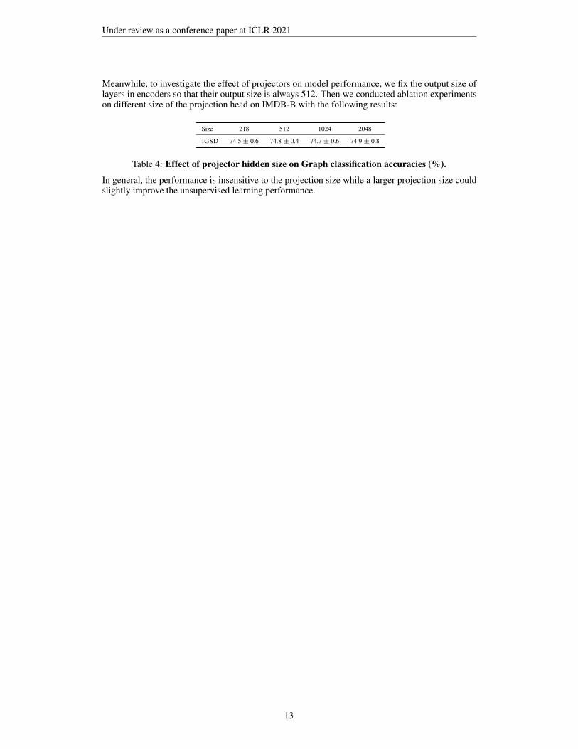
Meanwhile, to investigate the effect of projectors on model performance, we fix the output size oflayers in encoders so that their output size is always 512. Then we conducted ablation experimentson different size of the projection head on IMDB-B with the following results:

Size 218 512 1024 2048

IGSD 74.5± 0.6 74.8± 0.4 74.7± 0.6 74.9± 0.8

Table 4: Effect of projector hidden size on Graph classification accuracies (%).

In general, the performance is insensitive to the projection size while a larger projection size couldslightly improve the unsupervised learning performance.

13