0 Iterative Image Reconstruction Methods for Non-Cartesian MRI Jeff Fessler EECS Department Doug Noll BME Department The University of Michigan ISMRM Workshop on Non-Cartesian MRI Feb. 27, 2007 Acknowledgements: Brad Sutton
• “Non-Fourier” physical effects such as field inhomogeneity
• Incorporation of coil sensitivity maps
• Improved results for under-sampled trajectories (?)
• ...
(“Avoiding k-space interpolation” is not a compelling reason!)
3
Primary drawbacks of Iterative Methods
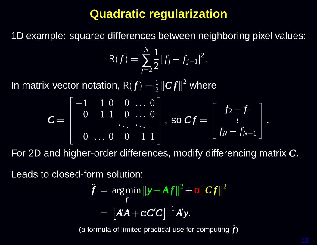
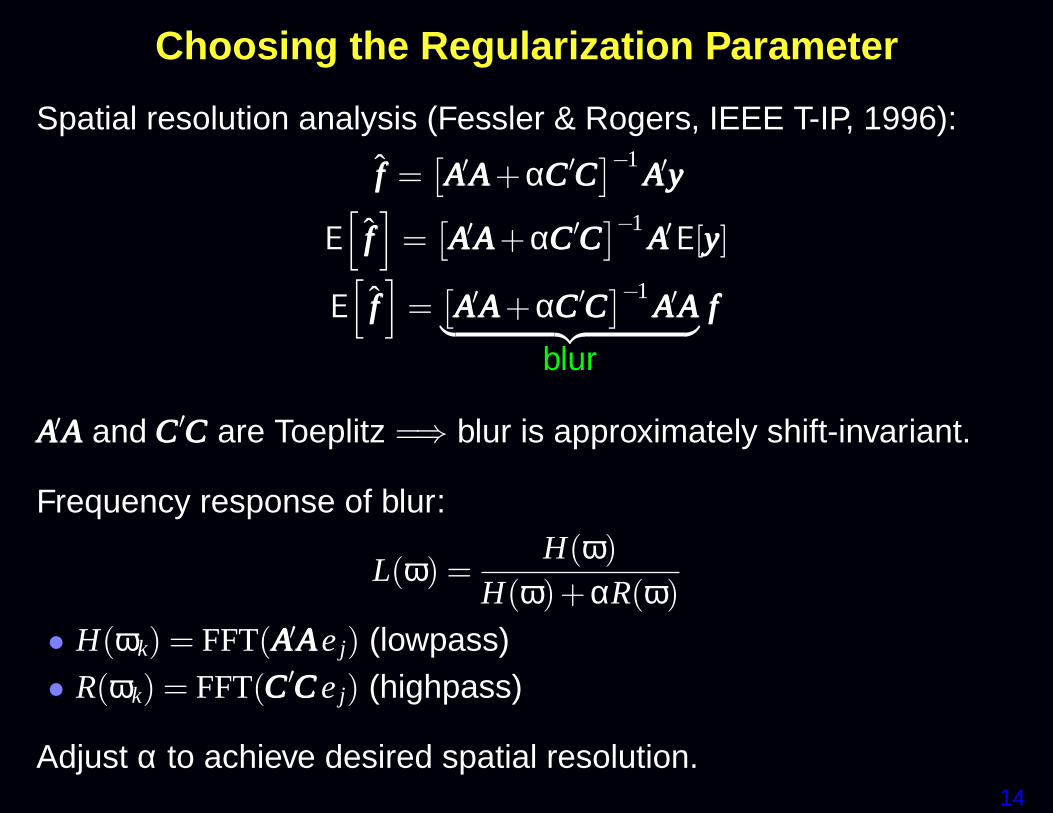
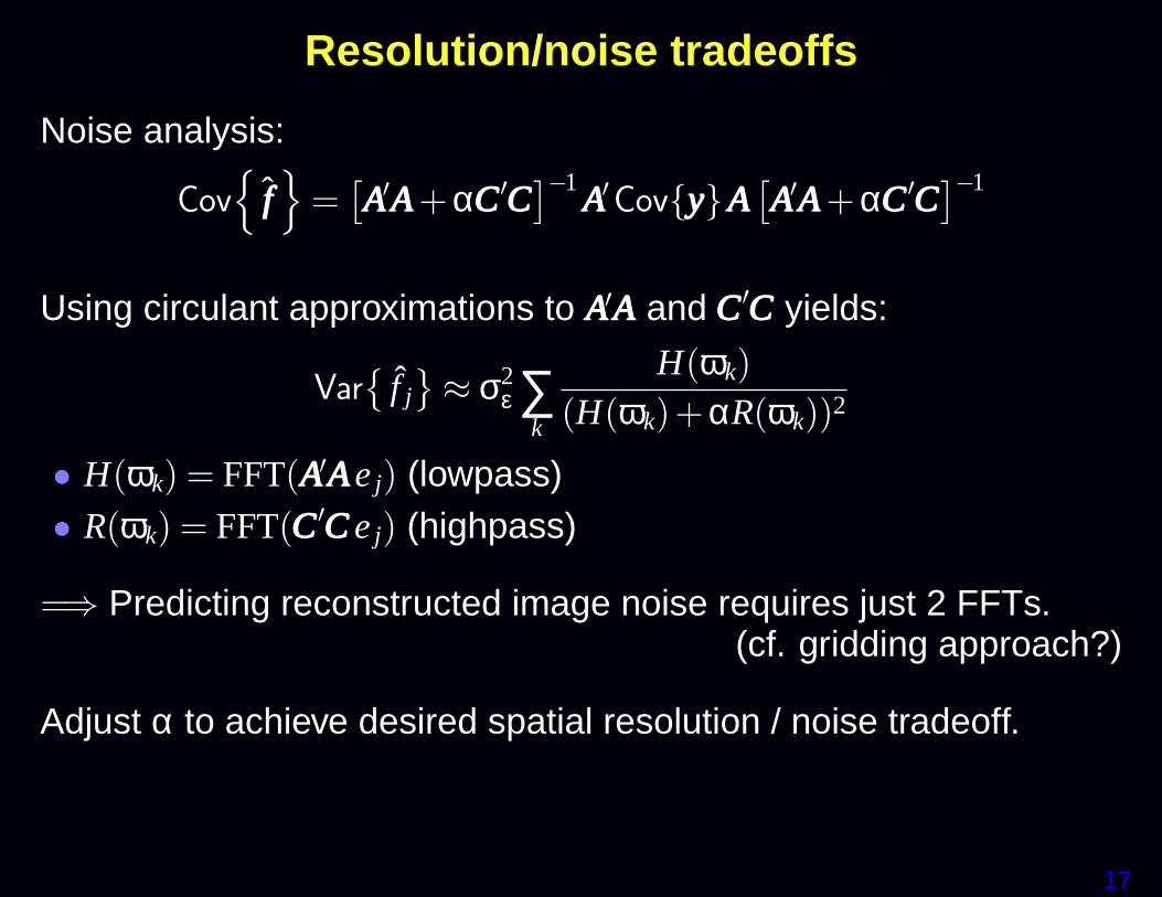
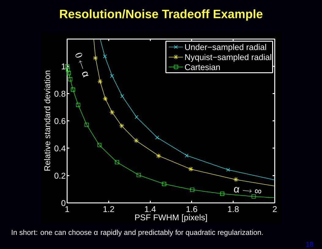
• Choosing regularization parameter(s)
• Algorithm speed
4
Introduction
5
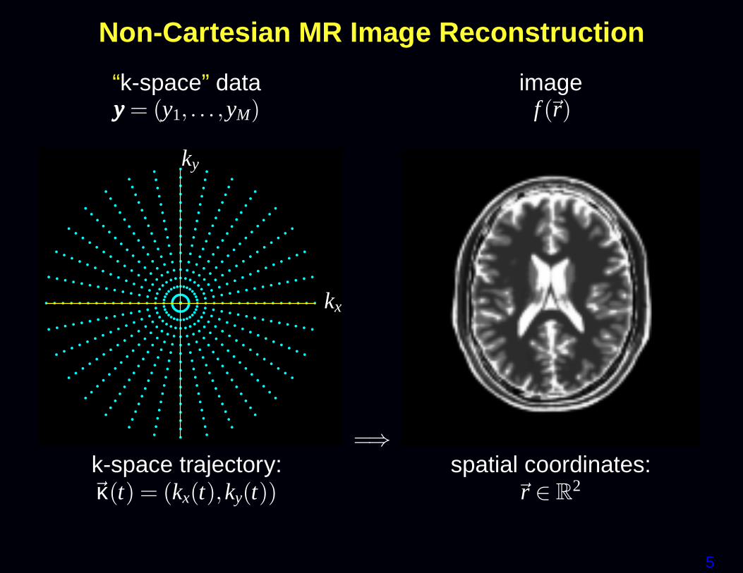
Non-Cartesian MR Image Reconstruction
“k-space” data imageyyy = (y1, . . . ,yM) f (~r)
kx
ky
=⇒k-space trajectory: spatial coordinates:~κ(t) = (kx(t),ky(t)) ~r ∈ R
2
6
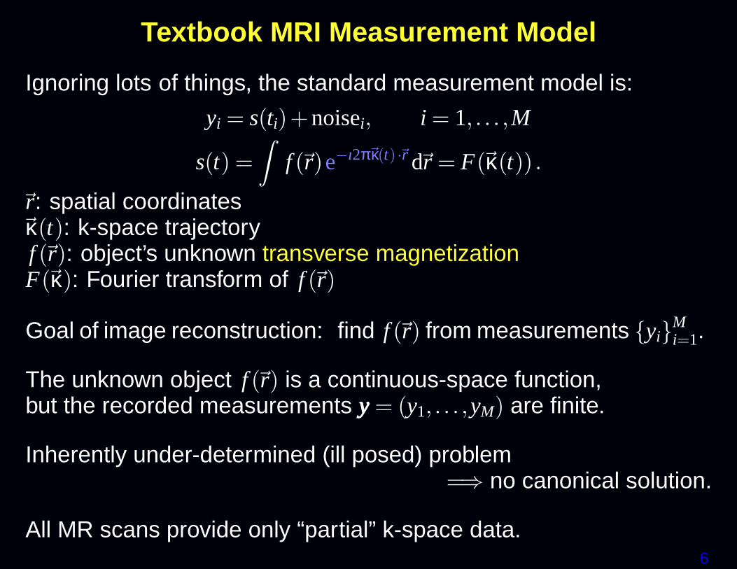
Textbook MRI Measurement Model
Ignoring lots of things, the standard measurement model is:
yi = s(ti)+noisei, i = 1, . . . ,M
s(t) =Z
f (~r)e−ı2π~κ(t) ·~r d~r = F(~κ(t)) .
~r: spatial coordinates~κ(t): k-space trajectoryf (~r): object’s unknown transverse magnetizationF(~κ): Fourier transform of f (~r)
Goal of image reconstruction: find f (~r) from measurements {yi}Mi=1.
The unknown object f (~r) is a continuous-space function,but the recorded measurements yyy = (y1, . . . ,yM) are finite.
Inherently under-determined (ill posed) problem=⇒ no canonical solution.
All MR scans provide only “partial” k-space data.
7
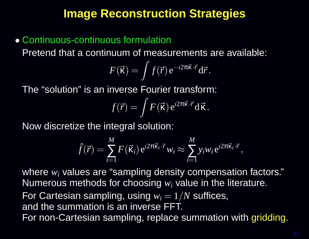
Image Reconstruction Strategies
• Continuous-continuous formulationPretend that a continuum of measurements are available:
F(~κ) =Z
f (~r)e−ı2π~κ ·~r d~r .
The “solution” is an inverse Fourier transform:
f (~r) =Z
F(~κ)eı2π~κ ·~r d~κ .
Now discretize the integral solution:
f̂ (~r) =M
∑i=1
F(~κi)eı2π~κi ·~r wi ≈M
∑i=1
yiwi eı2π~κi ·~r ,
where wi values are “sampling density compensation factors.”Numerous methods for choosing wi value in the literature.For Cartesian sampling, using wi = 1/N suffices,and the summation is an inverse FFT.For non-Cartesian sampling, replace summation with gridding.
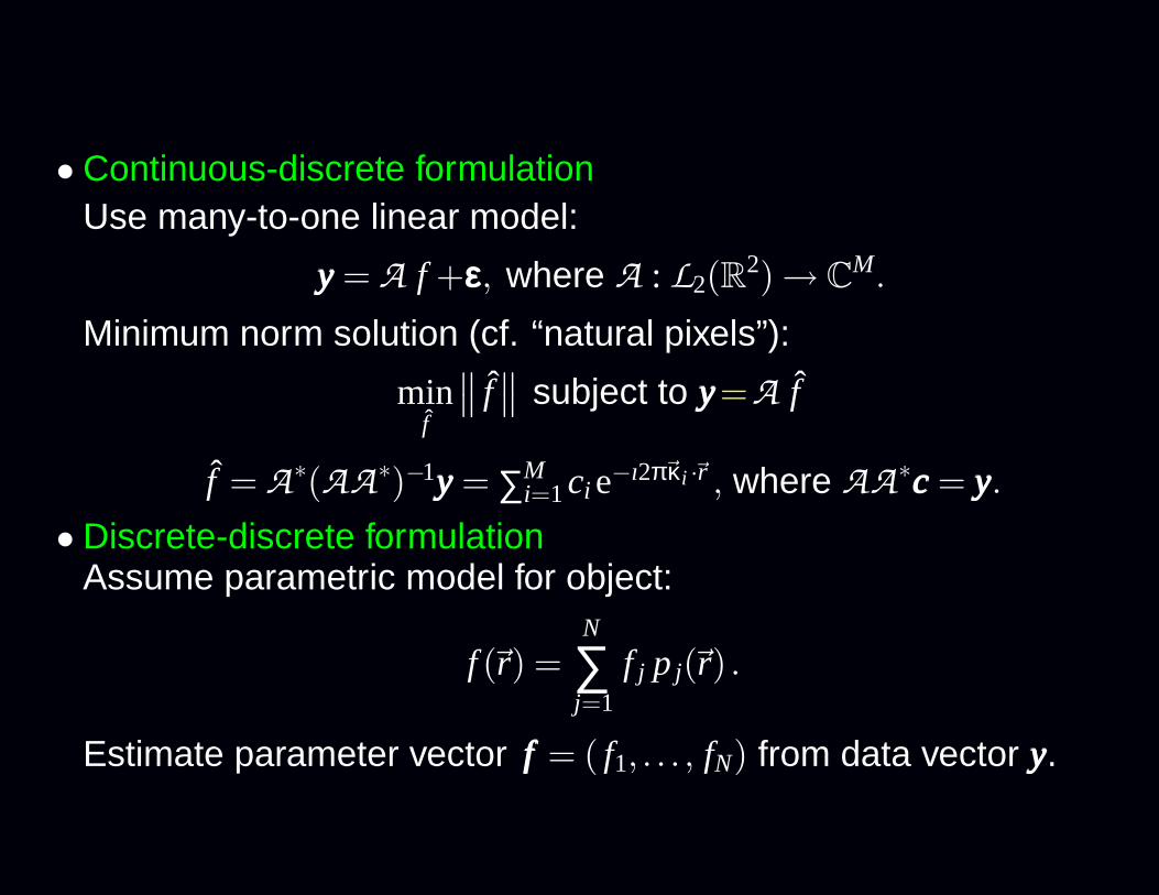
• Continuous-discrete formulationUse many-to-one linear model:
yyy = A f +εεε, where A : L2(R2)→ C
M.
Minimum norm solution (cf. “natural pixels”):
minf̂
∥∥ f̂
∥∥ subject to yyy=A f̂
f̂ = A∗(AA
∗)−1yyy = ∑Mi=1ci e−ı2π~κi ·~r , where AA
∗ccc = yyy.
• Discrete-discrete formulationAssume parametric model for object:
f (~r) =N
∑j=1
f j p j(~r) .
Estimate parameter vector fff = ( f1, . . . , fN) from data vector yyy.
9
Model-Based Image Reconstruction: Details
Substitute series expansion of unknown object:
f (~r) =N
∑j=1
f j p(~r−~r j)←− usually 2D rect functions
into signal model yi = s(ti)+ εi, where
E[yi] = s(ti) =Z
f (~r)e−ı2π~κi ·~r d~r,
yields:
E[yi] =Z
[N
∑j=1
f j p(~r−~r j)
]
e−ı2π~κi ·~r d~r =N
∑j=1
[Z
p(~r−~r j)e−ı2π~κi ·~r d~r
]
f j
=N
∑j=1
ai j f j, ai j = P(~κi)e−ı2π~κi ·~r j , p(~r)FT⇐⇒ P(~κ).
Discrete-discrete measurement model with system matrix AAA= {ai j}:
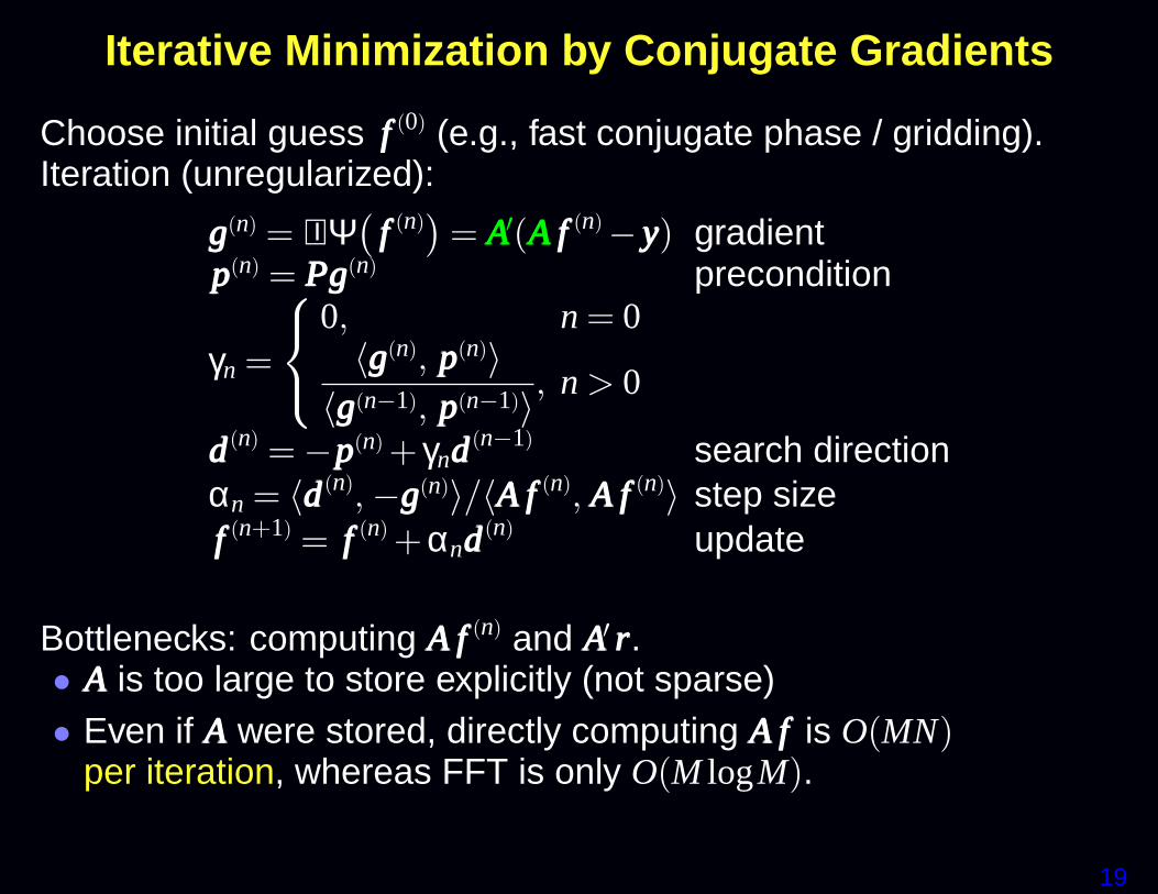
Bottlenecks: computing AAA fff (n) and AAA′ rrr.• AAA is too large to store explicitly (not sparse)• Even if AAA were stored, directly computing AAA fff is O(MN)
per iteration, whereas FFT is only O(M logM).
20
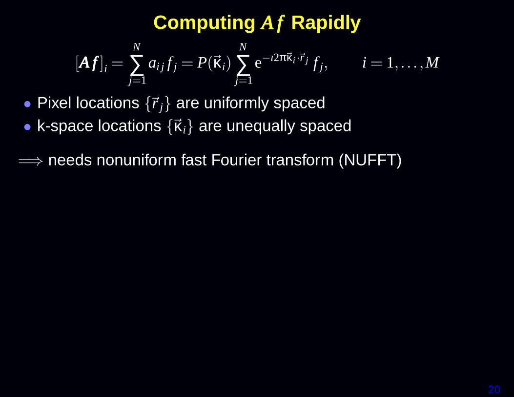
Computing AAA fff Rapidly
[AAA fff ]i =N
∑j=1
ai j f j = P(~κi)N
∑j=1
e−ı2π~κi ·~r j f j, i = 1, . . . ,M
• Pixel locations {~r j} are uniformly spaced• k-space locations {~κi} are unequally spaced
=⇒ needs nonuniform fast Fourier transform (NUFFT)
21
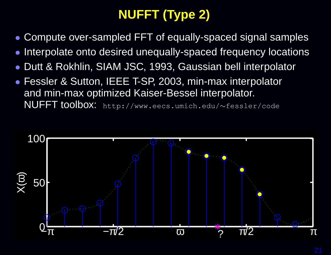
NUFFT (Type 2)
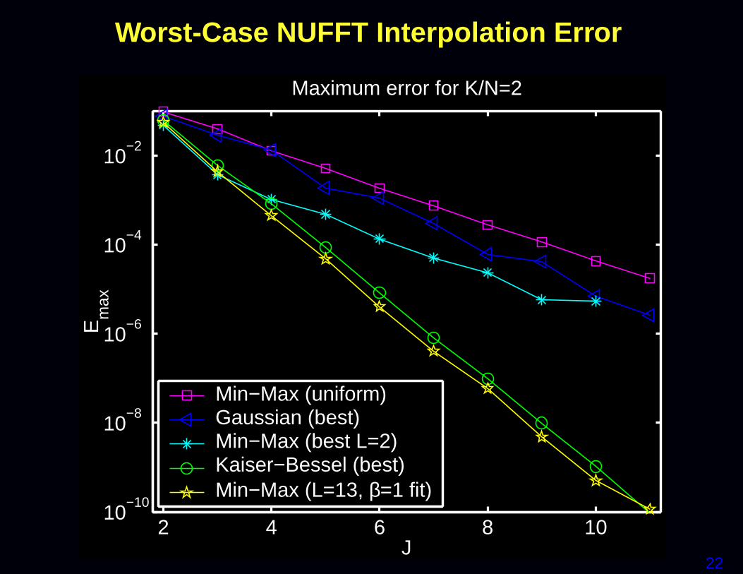
• Compute over-sampled FFT of equally-spaced signal samples• Interpolate onto desired unequally-spaced frequency locations• Dutt & Rokhlin, SIAM JSC, 1993, Gaussian bell interpolator• Fessler & Sutton, IEEE T-SP, 2003, min-max interpolator
and min-max optimized Kaiser-Bessel interpolator.NUFFT toolbox: http://www.eecs.umich.edu/∼fessler/code
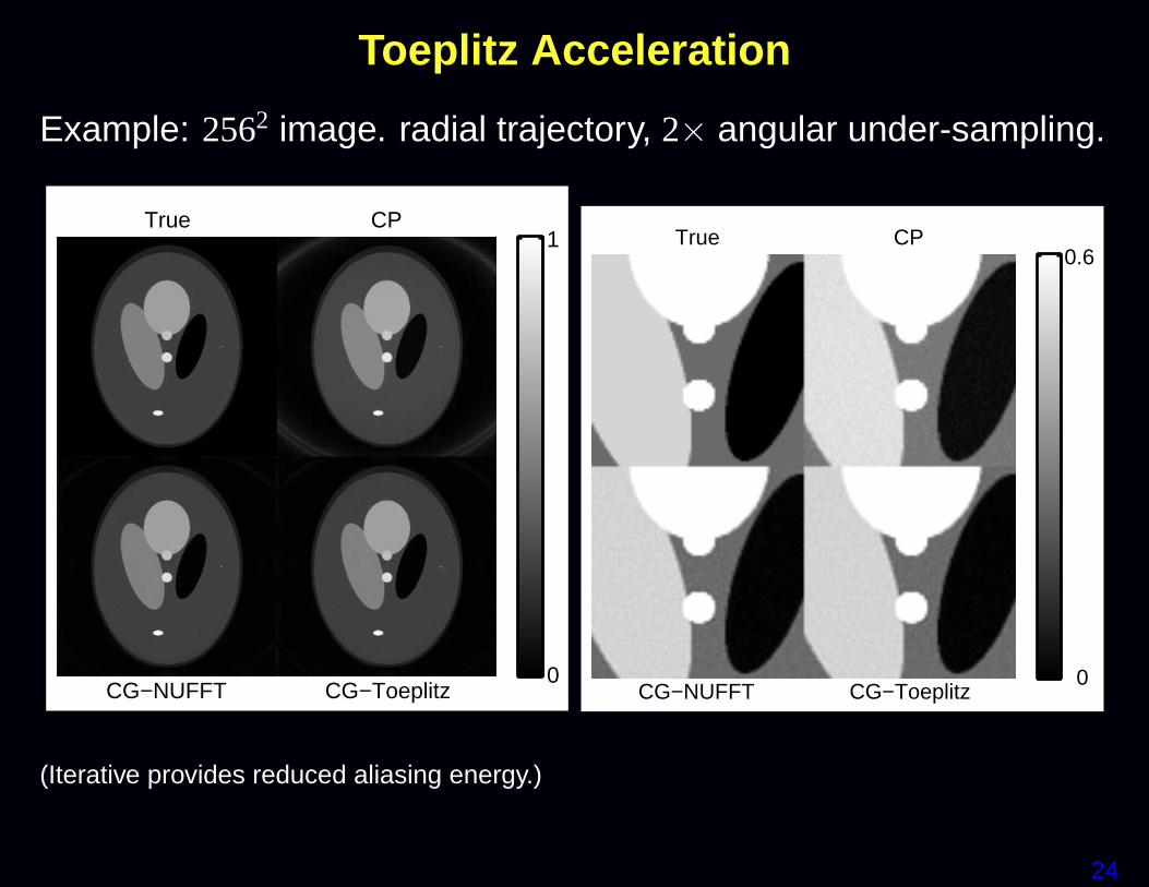
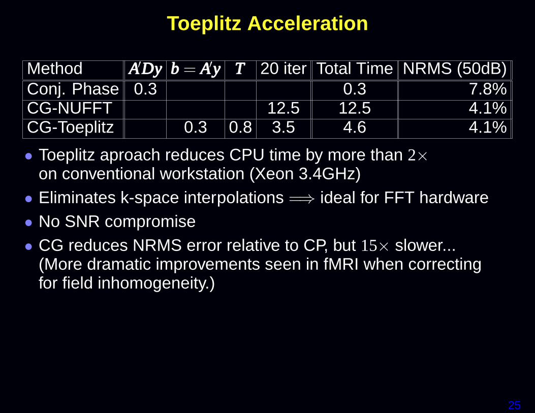
Method AAA′DDDyyy bbb = AAA′yyy TTT 20 iter Total Time NRMS (50dB)Conj. Phase 0.3 0.3 7.8%CG-NUFFT 12.5 12.5 4.1%CG-Toeplitz 0.3 0.8 3.5 4.6 4.1%
• Toeplitz aproach reduces CPU time by more than 2×on conventional workstation (Xeon 3.4GHz)• Eliminates k-space interpolations =⇒ ideal for FFT hardware• No SNR compromise• CG reduces NRMS error relative to CP, but 15× slower...
(More dramatic improvements seen in fMRI when correctingfor field inhomogeneity.)
26
Myths
• Choosing α is difficult
• Sample density weighting is desirable
27
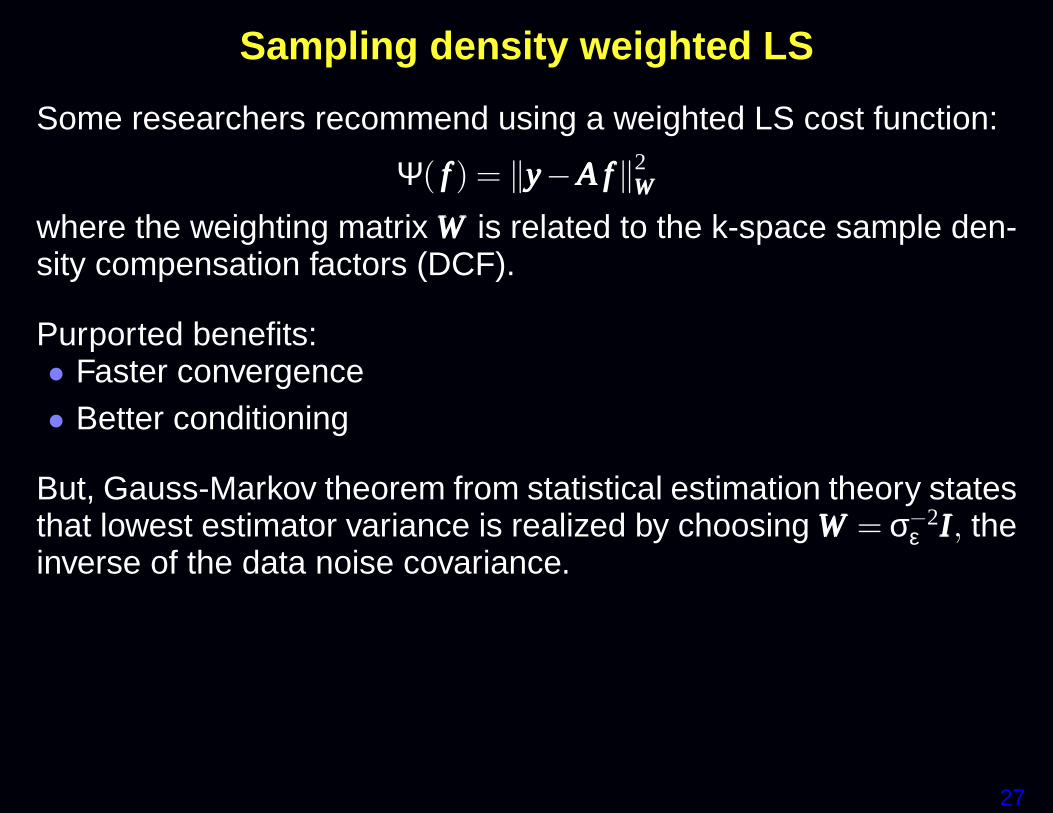
Sampling density weighted LS
Some researchers recommend using a weighted LS cost function:
Ψ( fff ) = ‖yyy−AAA fff‖2WWW
where the weighting matrix WWW is related to the k-space sample den-sity compensation factors (DCF).