Iterative learning controlforuncertain …mate.tue.nl/mate/pdfs/12012.pdf · Iterative Learning...

INTERNATIONAL JOURNAL OF ROBUST AND NONLINEAR CONTROLInt. J. Robust. Nonlinear Control (2010)Published online in Wiley Online Library (wileyonlinelibrary.com). DOI: 10.1002/rnc.1657

Iterative learning control for uncertain systems: Noncausal finitetime interval robust control design

J. J. M. van de Wijdeven, M. C. F. Donkers and O. H. Bosgra∗,†

Department of Mechanical Engineering, Eindhoven University of Technology,P. O. Box 513, 5600 MB Eindhoven, The Netherlands

SUMMARY

In this paper, we present a novel robust Iterative Learning Control (ILC) control strategy that is robustagainst model uncertainty as given by an additive uncertainty model. The design methodology hinges onH∞ optimization, but formulated such that the obtained ILC controller is not restricted to be causal,and inherently operates on a finite time interval. Optimization of the robust ILC (R-ILC) solution isaccomplished for the situation where any information about structure in the uncertainty is discarded,and for the situation where the information about the structure in the uncertainty is explicitly taken intoaccount. Subsequently, the convergence and performance properties of resulting R-ILC controlled systemare analyzed. On an experimental set-up, we show that the presented R-ILC control strategy can outperforman existing linear-quadratic norm-optimal ILC approach and an existing causal R-ILC approach based onfrequency domain H∞ synthesis. Copyright � 2010 John Wiley & Sons, Ltd.

Received 24 November 2008; Revised 4 August 2010; Accepted 9 August 2010

KEY WORDS: iterative learning control; robust control; uncertain systems

1. INTRODUCTION

Iterative Learning Control (ILC) is a control strategy used to improve the performance of batchrepetitive processes by iteratively updating the command signal from one batch (trial) to the next[1–4]. With this update based on measured data from previous trials, it can be considered aslearning from previous experience. Although the command signal generated by the ILC controlleris based on measured data, the controller is often designed using a model of the system. As nomodel can truly reflect the real system behavior, the controller is required to have some robustnessagainst model uncertainty. In this paper, we present a novel robust ILC (R-ILC) design strategythat is robust against trial invariant additive model uncertainty.

Robustness properties of common ILC control strategies, such as Arimoto gains, inverse modelILC, and linear-quadratic (LQ) norm-optimal ILC have been discussed in the ILC literature. Forinstance, in [5] it is shown that there exist inverse model ILC controllers for which the ILCcontrolled system is robustly monotonically convergent (RMC), if the uncertainty is restricted tomultiplicative descriptions that are positive real. In [6], robustness of LQ norm-optimal ILC isstudied over the finite time interval of a trial for multiplicative uncertainty models which canbe represented by a gain. Robustness of LQ norm-optimal ILC, as discussed in [7], is basedon a frequency domain representation of the ILC controller. Consequently, the results are only

∗Correspondence to: O. H. Bosgra, Eindhoven University of Technology, WH-1.145, P. O. Box 513, 5600 MBEindhoven, The Netherlands.

†E-mail: [email protected]

Copyright � 2010 John Wiley & Sons, Ltd.

J. J. M. VAN DE WIJDEVEN, M. C. F. DONKERS AND O. H. BOSGRA

approximate since ILC controllers inherently act on a finite time interval. Namely, the Fouriertransform on the infinite time interval used for this approach leads to a linear time invariant (LTI)control law. Application of this LTI controller on the finite time interval of a trial may result inerrors in the initial part of the transient behavior (which is shown in Section 6 on an example). In[8], the finite interval representation of the system and controllers is approximated in a Fourier basisleading to an unclear definition of the uncertainty model and a number of approximate robustnessresults. Finally, in [9, 10], the finite-time interval aspect of ILC is explicitly included in the robustconvergence analysis. However, the approach does not leave room to include uncertainty models.As a result, the robustness properties of the solution cannot be quantified.

In contrast to analysis of given ILC control strategies with respect to robustness, there alsoexist R-ILC design strategies that incorporate an uncertainty model in the design procedure so asto improve the robustness and performance of the ILC controlled system. In [11, 12], the robustcontrol design problem is discussed in a 2D system representation, and yields a combined statefeedback controller in time domain and Arimoto gain ILC controller in trial domain. Hence, fullknowledge of the time domain system states is required. In [13–17], the design problem is posedas an H∞ optimization problem in frequency domain, and therefore yields an approximate resultsince again the Fourier transform assumes the signals to be given on an infinite time interval.Moreover, the resulting H∞ optimal controllers are causal, i.e. the command signal in trial k+1at time t∗ only depends on information about trial k at time samples t={0,1, . . . , t∗}. As a result,these papers do not allow the ILC controller to be noncausal. Finally, in [18], the ILC designproblem is formulated as a causalH∞ problem in the trial domain. In contrast, this paper focusseson noncausal R-ILC control design over a finite time interval.

R-ILC control design for systems with interval uncertainty is studied in [19]. The resultingcontroller is noncausal and inherently acts on a finite time interval. The uncertainty model usedputs an individual error bound on each element of the impulse response, which leads to a largecomputational burden for any realistic problem. In this paper, a different model is used. In [6],a min–max optimization problem is formulated to solve a constrained R-ILC control problemfor systems under worst case trial varying uncertainty. Owing to the constrained R-ILC controlproblem formulation, no analytical solution for the ILC controller can be given. Moreover, thesolution is computationally demanding.

On the basis of the discussion so far, we can indicate key issues in R-ILC control design inthe presence of model uncertainty: (i) inclusion of the finite time interval aspect of a trial (for anaccurate representation of the ILC problem), (ii) allowance of noncausal robust control solutions(for generality of the solution), (iii) inclusion of an uncertainty model in the ILC design process(for quantification of the robustness properties and improvement of achievable performance), and(iv) existence of an analytical solution for the R-ILC controller (for ease of implementation). Thepreviously discussed approaches cover one or more of these issues. However, to the best of ourknowledge, none incorporates all aspects.

In this paper, we present a solution to all of the four issues in a novel R-ILC design strategywhich utilizes an additive model uncertainty representation in the design process. To obtain ananalytical solution for the R-ILC design problem, we use H∞ optimization for discrete timesystems, however, formulated such that the solution is not constrained to be causal and inherentlyacts on a finite time interval. Optimization of the R-ILC solution is performed for two cases: (i)where any information about structure in the uncertainty is discarded and (ii) where informationabout structure in the uncertainty is taken into account. Experimental results of R-ILC on a flexiblemechanical system illustrate that the suggested R-ILC controller can outperform LQ norm-optimalILC and frequency domain causal R-ILC.

This paper is organized as follows. In Section 2, we introduce the notions of robust mono-tonic convergence and performance in ILC. Subsequently, a sub-optimal R-ILC design problem isformulated and solved in Section 3. In Section 4, optimized finite interval R-ILC control solutionsfor the sub-optimal R-ILC controller are presented, after which the performance and convergenceproperties of the optimized R-ILC controlled system are discussed in Section 5. In Section 6,the derived R-ILC controller is compared experimentally with an existing LQ norm-optimal ILC

Copyright � 2010 John Wiley & Sons, Ltd. Int. J. Robust. Nonlinear Control (2010)DOI: 10.1002/rnc

NONCAUSAL FINITE TIME INTERVAL ROBUST ILC CONTROL DESIGN

controller and frequency domain causal R-ILC controller, and it is shown that the newly proposedcontroller outperforms them. Finally, concluding remarks are given in Section 7.

DefinitionsThe 2-norm of a vector p is given by ‖p‖2=

√pT p. The induced 2-norm of a finite dimensional

system matrix P is given by ‖P‖i2=�(P), with �(P) as the largest singular value of P . Theinduced 2-norm of P(z) is given by ‖P(z)‖i2=max�∈[−�,�] �(P(e j�)) with � real valued. Thekernel of a matrix A is given by ker(A) :={x : Ax=0}. Finally, ε is an arbitrarily small positivescalar: 0<ε�1.

2. PRELIMINARIES

In this section, we introduce the finite time interval uncertain model representation and ILC controlframework and discuss the issues of robust monotonic convergence and performance.

The finite time interval system representation follows from infinite time system descriptionwhich is assumed to be defined by a real rational discrete time transfer function P(z) that is causalin the shift operator z. Given a time signal y(t), z is defined as y(t+1)= zy(t). Consequently, P(z)has discrete time domain inputs and outputs defined over the time axis t ∈Z.

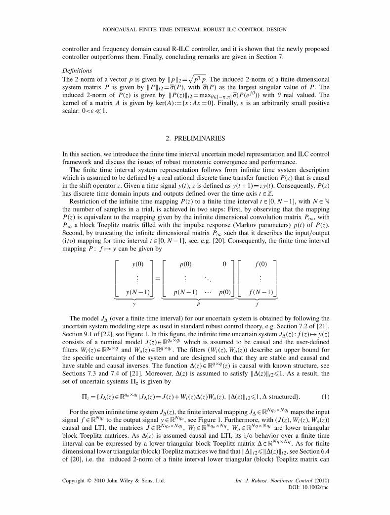
Restriction of the infinite time mapping P(z) to a finite time interval t ∈ [0,N−1], with N ∈N

the number of samples in a trial, is achieved in two steps: First, by observing that the mappingP(z) is equivalent to the mapping given by the infinite dimensional convolution matrix P∞, withP∞ a block Toeplitz matrix filled with the impulse response (Markov parameters) p(t) of P(z).Second, by truncating the infinite dimensional matrix P∞ such that it describes the input/output(i/o) mapping for time interval t ∈ [0,N−1], see, e.g. [20]. Consequently, the finite time intervalmapping P : f �→ y can be given by⎡

⎢⎢⎢⎣y(0)

...

y(N −1)

⎤⎥⎥⎥⎦

︸︷︷︸y

=

⎡⎢⎢⎢⎣

p(0) 0

.... . .

p(N−1) · · · p(0)

⎤⎥⎥⎥⎦

︸︷︷︸P

⎡⎢⎢⎢⎣

f (0)

...

f (N−1)

⎤⎥⎥⎥⎦

︸︷︷︸f

The model J� (over a finite time interval) for our uncertain system is obtained by following theuncertain system modeling steps as used in standard robust control theory, e.g. Section 7.2 of [21],Section 9.1 of [22], see Figure 1. In this figure, the infinite time uncertain system J�(z) : f (z) �→ y(z)consists of a nominal model J (z)∈Rqo×qi which is assumed to be causal and the user-definedfilters Wi (z)∈Rqo×q and Wo(z)∈Rq×qi . The filters (Wi (z),Wo(z)) describe an upper bound forthe specific uncertainty of the system and are designed such that they are stable and causal andhave stable and causal inverses. The function �(z)∈Rq×q(z) is causal with known structure, seeSections 7.3 and 7.4 of [21]. Moreover, �(z) is assumed to satisfy ‖�(z)‖i2�1. As a result, theset of uncertain systems �z is given by

�z ={J�(z)∈Rqo×qi |J�(z)= J (z)+Wi (z)�(z)Wo(z),‖�(z)‖i2�1,� structured}. (1)

For the given infinite time system J�(z), the finite interval mapping J� ∈RNqo×Nqi maps the inputsignal f ∈RNqi to the output signal y∈RNqo , see Figure 1. Furthermore, with (J (z),Wi (z),Wo(z))causal and LTI, the matrices J ∈RNqo×Nqi , Wi ∈RNqo×Nq , Wo ∈RNq×Nqi are lower triangularblock Toeplitz matrices. As �(z) is assumed causal and LTI, its i/o behavior over a finite timeinterval can be expressed by a lower triangular block Toeplitz matrix �∈RNq×Nq . As for finitedimensional lower triangular (block) Toeplitz matrices we find that ‖�‖i2�‖�(z)‖i2, see Section 6.4of [20], i.e. the induced 2-norm of a finite interval lower triangular (block) Toeplitz matrix can



Figure 1. (Left) Infinite time uncertain system J�(z) and (Right) uncertainsystem J� over a finite time interval.

Figure 2. ILC control framework in trial domain, with ILC controller (Q,Lo,Lc).

never exceed the induced 2-norm of the underlying transfer function, the set of uncertain systemsover a finite time interval can be given by

�={J� ∈RNqo×Nqi |J� = J+Wi�Wo,�∈D}, (2)

in which D={�∈RNq×Nq |‖�‖i2�1,� structured}.For ILC control, we focus on the ILC control framework consisting of the uncertain system J�

and ILC controller (Q, Lo, Lc), as depicted in Figure 2. In this figure, ek = yd− J�Lcuk representsthe error signal with yd ∈RNqo the reference signal, k∈N∪{0} the trial index, uk ∈Rp the trial statewith p= rank(J ), and w−1 :uk =w−1uk+1 the one-trial shift operator. Moreover, from Figure 2 itfollows that the used ILC control strategy corresponds to

uk+1=Quk+Loek, fk = Lcuk, u0=0, (3)

with Q∈Rp×p , Lo∈Rp×Nqo , and Lc∈RNqi×p . After substituting ek = yd− J�Lcuk in (3), weobtain the trial domain behavior

uk+1= (Q−Lo J�Lc)uk+Loyd . (4)

The ILC controlled system represented by (4) is robustly convergent (RC) iff |�i (Q−Lo J�Lc)|<1∀J� ∈�, i ={1,2, . . . , p}. Although this formulates a necessary and sufficient condi-tion for convergence of (4), mere convergence of (4) can lead to undesirable transient behaviorof the input and error signals in trial domain, [23], e.g. the maximum amplitude of the timesignals during a trial can become unacceptably high. To avoid this behavior, we require that (4)is monotonically convergent.

In this paper, two definitions for monotonic convergence are considered: nominal monotonicconvergence of (4) with J� = J∀�∈D, i.e. with Wi =0 and Wo=0, and robust monotonic conver-gence of (4) for given J� ∈�.

Definition 1 (Nominal Monotonic Convergence (NMC))Given ILC controller (3) and the ILC controlled system (4) with J� = J∀�∈D, yd =0, and u0∈Rp .Then (4) is NMC in fk if there exists 0��<1 such that

‖ fk+1‖2��‖ fk‖2 ∀k�0 and ∀u0∈Rp. (5)

From Definition 1, the following NMC condition can be derived.



Lemma 1Consider the nominal ILC controlled system (4), i.e. (4) with J� replaced by J and yd =0.Furthermore, let T satisfy T TLT

c LcT = Ip . Then (4) is NMC in fk if ‖T−1(Q−Lo J Lc)T ‖i2<1.

ProofSee Appendix A.1, which originates from [24]. �

The matrix T can be obtained by factorizing LTc Lc using, e.g. a Cholesky decomposition. Lemma 1

states that for trial state zk =T−1uk , NMC of zk implies NMC of the input signal fk .The introduction of model uncertainty in the ILC controlled system leads to the following robust

monotonic convergence definition.

Definition 2 (RMC)Given ILC controlled system (4) and ILC controller (3), with yd =0 and u0∈Rp . Then (4) is RMCin fk if there exists 0��<1 such that

‖ fk+1‖2��‖ fk‖2 ∀k�0 ∀u0∈Rp and ∀J� ∈�. (6)

Based on Definition 2, the following RMC condition is obtained.

Lemma 2Consider the ILC controlled system (4) with yd =0. Furthermore, let T satisfy T TLT

c LcT = Ip .Then (4) is RMC in fk if ‖T−1(Q−Lo J�Lc)T ‖i2<1 ∀J� ∈�.

ProofFollows the same line of reasoning as the proof of Lemma 1. �

Remark 1In this paper, the derived NMC and RMC conditions are based on Definitions 1 and 2. Alternatively,the same NMC and RMC conditions can be obtained by considering yd �=0 and u0=0. For yd �=0and u0=0, (robust) monotonic convergence requires ‖ fk+1− f∞‖2<‖ fk− f∞‖2∀k�0 (∀J� ∈�)with f∞ = limk→∞ fk .

Remark 2It is very common in the ILC literature to take Lc= Ip (and hence assume rank(J )= p=Nqi ).However, consider the case (Q, Lc)= (INqi , INqi ) and rank(J )<Nqi . Then independent of the choicefor Lo there will be �i (Lo J Lc)=0 for some i . As convergence requires |�i (INqi −Lo J Lc)|=|1−�i (Lo J Lc)|<1, convergence cannot be achieved for (Q, Lc)= (INqi , INqi ) and rank(J )<Nqi .This convergence issue can, however, be resolved by factorizing J using a full rank decomposition

J = Jo Jc with Jo∈RNqo×p, Jc∈Rp×Nqi ,

rank(Jo)= rank(Jc)= rank(J )= p, (7)

subsequently defining Lc := J †c = JTc (Jc JTc )

−1 and Q= Ip , and finally designing Lo using systemJo. The case Lc �= I is discussed extensively in [25, 26].

In this paper, we assume Lc= INqi to keep notations and derivations for R-ILC as simple aspossible. As a result, fk =uk and T = I . It is, however, straightforward to extend the presentedresults to cases where Lc �= INqi .

Conclusively, we address the notion of performance in ILC.

Definition 3 (Performance)The ILC controlled system (4) is said to have performance ‖e∞‖2, with e∞ = limk→∞ ek theasymptotic error.



Lemma 3Given an ILC controlled system (4), and assume that (4) is RC. Then e∞ =0 for any yd iffrank(J�)= p=Nqo∀J� ∈� and Q= Ip .

ProofFollows from [27]. �

With Lc= Ip , Lemma 3 states that e∞ =0 for any yd if and only if p=Nqo=Nqi∀J� ∈�.

3. SUB-OPTIMAL NONCAUSAL FINITE TIME INTERVAL R-ILC CONTROL DESIGN

In this section, we derive a sub-optimal finite time interval R-ILC controller using the uncertainsystem description introduced in the previous section. For this, we apply H∞ control theory fordiscrete time systems, [28, 29], but formulated such that the controller is not restricted to be causaland operates on a finite time interval. As the Hardy space refers to a class of stable, causal transferfunctions, the name H∞ is not appropriate for the presented solution.

3.1. Existence conditions for a sub-optimal finite interval robust control problem

The approach taken here is to formulate the problem using the generalized plant paradigm, asdepicted in Figure 3. In this figure, the signalwo(t) is referred to as exogenous input, and can includereference signals, noise signals, disturbance signals, etc. The signal zo(t) contains the performancevariables, e.g. command signals and error signals. The signal y(t) denotes the controller input,u(t) is the controller output, and q(t) and p(t) are the input and output signals of the normalizeduncertainty block �G , respectively.

For a given generalized plant G with w(t) := [pT(t) wTo (t)]

T and z(t) := [qT(t) zTo (t)]T, the finite

time interval robust control problem consists of finding a robust controller K generating a controlsignal u(t) for t ∈ [0,N−1] which minimizes the induced 2-norm of the mapping M :w(t) �→ z(t),subject to a worst case disturbance w(t), [28, 29]. The induced 2-norm of M with the optimizedcontroller K is given by

�opt=minu(t)

maxw(t)

‖M‖i2, t ∈ [0,N−1]. (8)

As the solution of (8) is in general difficult to obtain, see, e.g. [22], we focus on finding asolution to a sub-optimal robust control problem for �>�opt. The bound � can be made arbitrarilytight by using a bisection algorithm, see, e.g. [21, 22]. For that purpose, let the vectors (z,w,u, y)represent the finite time interval signals (z(t),w(t),u(t), y(t)) for t=0, . . . ,N−1. Furthermore,consider the generalized plant [

z

y

]=

[G11 G12

G21 0

][w

u

]. (9)

Figure 3. Generalized plant formulation with generalized plant G , controllerK , and norm bounded uncertainty �G .



Then the finite interval sub-optimal robust control problem can be given by

minu

maxw

J with

J= 12 (G11w+G12u)

T(G11w+G12u)− 12�

2wTw+�T(y−G21w), (10)

where � is a Lagrange multiplier. See Appendix A.2 for the derivation of (10).To formulate existence conditions for the sub-optimal problem (10), i.e. the conditions which

guarantee the existence of a unique solution to the optimization problem (10), we require thefollowing result.

Lemma 4Given the optimization problem

maxx

12 x

TQx+cTx subject to Ax=b,

with A a fat matrix, i.e. with A∈Rn×m , m>n. This optimization problem has a unique solution ifA has full row rank and if xTQx<0 for all x ∈ker(A).

ProofSee Sections 10.3 and 14.1 in [30]. �

Based on Lemma 4, the existence conditions for (10) can be posed.

Corollary 1Given �, then there exists a solution for (10) being a saddle point of J, if G12 has full columnrank, G21 has full row rank, and xT(GT

11G11−�2 I )x<0 for all x ∈ker(G21).

Note that existence of a unique solution for (10), i.e. the saddle point, does not necessarilyimply that ‖M‖i2<�. This issue is discussed in Section 4.

3.2. Choices for performance and control structure

In the previous section, we introduced the sub-optimal finite interval robust control problem for anarbitrary generalized plant G. In this section, we formulate a specific generalized plant. This plantis used for the derivation of the noncausal finite time interval R-ILC controller in Section 3.3.

The expression for the generalized plant description with variables (z, y,w,u) results from theformulation of the performance variables zo, external inputs wo, model uncertainty p and q, andcontrol structure u and y. The first performance objective in our sub-optimal robust control problemaims at the minimization of the error during trial k+1, i.e. minimization of ek+1. Using the factthat ek = yd − J fk−Wi pk , the error ek+1 can be given by

ek+1=ek+ J ( fk − fk+1)+Wi (pk− pk+1). (11)

The second performance objective focusses on penalizing the changes of the command signal fromone trial to the next, i.e. on f� = fk+1− fk , using a positive definite weight R with factorization

R= (R12 )TR

12 . Penalizing f� can be beneficial for performance in case of trial varying disturbances,

see [26, 31]. The desired control structure is given by (3) with Lc= I . As a result fk =uk . Finally,with ek+1 a function of both pk and pk+1, and with pk =� qk and pk+1=�qk+1, �G in Figure 3is defined as �G :=diag(�,�) with inputs qk and qk+1.

Based on the previous discussion, (z, y,w,u) are given by

z = [qTk qTk+1 eTk+1 f T� ]T (12a)

y = [eTk f Tk ]T (12b)

w = [pTk pTk+1 eTk f Tk ]T (12c)

u = fk+1. (12d)



Figure 4. Generalized plant formulation for the R-ILC problem.

Moreover, the generalized plant G is defined by (13), see also Figure 4.⎡⎢⎢⎢⎢⎢⎢⎢⎢⎢⎢⎣

qk

qk+1

ek+1

f�

ek

fk

⎤⎥⎥⎥⎥⎥⎥⎥⎥⎥⎥⎦

=

⎡⎢⎢⎢⎢⎢⎢⎢⎢⎢⎢⎢⎣

0 0 0 Wo 0

0 0 0 0 Wo

Wi −Wi I J −J

0 0 0 −R12 R

12

0 0 I 0 0

0 0 0 I 0

⎤⎥⎥⎥⎥⎥⎥⎥⎥⎥⎥⎥⎦

︸︷︷︸G

⎡⎢⎢⎢⎢⎢⎢⎢⎢⎣

pk

pk+1

ek

fk

fk+1

⎤⎥⎥⎥⎥⎥⎥⎥⎥⎦

. (13)

3.3. Solution of the sub-optimal robust control problem

In Corollary 2, the existence conditions for the robust control problem with generalized plant (13)are derived.

Corollary 2Given the sub-optimal finite interval robust control problem (10) for generalized plant (13). Thereexists a unique solution for (10) if �>

√2‖Wi‖i2.

ProofSee Appendix A.3. �

With the generalized plant and existence conditions given, the solution to (10) is given in thefollowing proposition.

Proposition 1Given (12) and (13), and �>

√2‖Wi‖i2, then the controller that solves (10) is given by

Q= (JTQJ+S+R)−1(JTQJ+R), (14a)

Lo = (JTQJ+S+R)−1 JTQ, (14b)

with

Q= (I−2�−2WiWTi )

−1 and S=WTo Wo. (15)

ProofSee Appendix A.4. �

Note the difference between ILC control element Q and weighting matrix Q. Moreover, notethat the existence condition �>

√2‖Wi‖i2 is equivalent to the condition Q 0.



With Q and Lo both a function of the upper triangular block Toeplitz matrix JT, the obtainedILC controller is not restricted to be causal.

4. OPTIMIZED FINITE INTERVAL R-ILC CONTROL SOLUTIONS

In Section 3, the solution to the sub-optimal finite interval R-ILC control problem for given � hasbeen presented. In this section, two optimized solutions for the finite interval robust control problemare derived. Both solutions are obtained by optimizing the sub-optimal solution of Section 3 withrespect to �. In Section 4.1, optimization of the R-ILC solution is accomplishedwhile discarding anyinformation about structure in the uncertainty, i.e. by considering the uncertainty to be unstructured.This approach is comparable to conventional H∞ control synthesis. In Section 4.2, an optimizedsolution is obtained by explicitly taking into account the information about the structure in theuncertainty. This approach is comparable to so-called �-synthesis, see e.g. [21, 22].

4.1. Optimized finite interval robust control for unstructured uncertainty

Optimization of the R-ILC controller over � is based on the mapping M :w �→ z and norm-boundeduncertainty �M : z �→w. For the R-ILC control problem of Section 3, system M is obtained byclosing the loop between G and (Lo,Q), see Figure 3 and (16).

⎡⎢⎢⎢⎢⎣

qk

qk+1

ek+1

f�

⎤⎥⎥⎥⎥⎦=

⎡⎢⎢⎢⎢⎢⎣

0 0 0 Wo

0 0 WoLo WoQ

Wi −Wi I− J Lo J (I −Q)

0 0 R12 Lo R

12 (Q− I )

⎤⎥⎥⎥⎥⎥⎦

︸︷︷︸M

⎡⎢⎢⎢⎢⎣

pk

pk+1

ek

fk

⎤⎥⎥⎥⎥⎦ . (16)

The uncertainty �M is an element of the set

DM ={�M =diag(�G ,�P )=diag(�,�,�P )|�∈D,�P ∈DP}, (17)

with DP ={�P ∈RN (qi+qo)×N (qi+qo)|‖�P‖i2�1}. In (17), �G : [qTk qTk+1]T �→ [pTk pTk+1]

T followsfrom Figure 4, and �P is an unstructured uncertainty which maps zo= [eTk f Tk ]

T to wo=[eTk+1 f T� ]

T.In this section, the uncertainty �M is assumed to be unstructured. As a result, optimization

of the R-ILC controller over � consists of finding an approximation for �opt, while satisfying‖M‖i2<�. As stated in, e.g. Section 9.3 of [21], the approximation of �opt, denoted by �min, canbe derived using a bisection algorithm. The obtained �min lies within a user defined bound ε of�opt: �opt<�min<�opt+ε, such that ‖M‖i2<�min.

4.2. Optimized finite interval robust control for structured �M

To exploit the information about the structure of �M in the optimization procedure, a scalingmatrix DM is introduced in the control loop, see Figure 5.

Given �M of (17), matrix DM is chosen to be an element of the set

DM = {DM =diag(D1,D1, IN (qi+qo))|D1∈RNq×Nq ,DM�M =�MDM ,

rank(DM )=N (qi +qo+2q),�M ∈DM },see, e.g. [32]. For DM ∈DM , we obtain ‖D−1

M �MDM‖i2=‖D−1M DM�M‖i2=‖�M‖i2. Conse-

quently, DM does not alter the norm properties of �M . On the other hand, in general ‖M‖i2 �=‖DMMD−1

M ‖i2. Matrix DM can hence be exploited to find a ‖DMMD−1M ‖i2 which is smaller than

‖M‖i2.



Figure 5. M�M structure.

For given DM and given �, we first consider the sub-optimal finite interval R-ILC controlsolution, Proposition 2.

Proposition 2Given DM , and generalized plant (13) with G11 replaced by DMG11D

−1M . Furthermore, let

�>√2‖WiD

−11 ‖i2. Then the controller that solves (10) is given by (14) with

Q= (I−2�−2WiD−11 D−1T

1 WTi )

−1 and S=WTo D

T1 D1Wo. (18)

ProofThe existence condition follows from Corollary 2. The solution for (Q, S) follows from Proposi-tion 1 where G11 in (13) is replaced by DMG11D

−1M . �

In Proposition 3, an algorithm is given for optimization of the sub-optimal R-ILC controller ofProposition 2 over � and DM . This algorithm is comparable to the DK-iteration in time domain�-synthesis, see e.g. Section 8.12 in [21] and Section 11.4 in [22].

Proposition 3Given generalized plant G of (13), uncertainty �M ∈DM of (17), and R-ILC controller (Lo,Q)from (14). Furthermore, let DM ∈DM . Optimizing (Lo,Q) comprises the following steps:

Initialization: DM = I .

1. Given DM , and M which is obtained from (13) with G11 replaced by DMG11D−1M and

(Lo,Q) of (14) with (Q, S) from (18). Find �min, e.g. using a bisection algorithm.2. For given �min and M , find DM ∈DM such that ‖DMMD−1

M ‖i2 is minimized.3. Return to step 1. until either (i) ‖DMMD−1

M ‖i2 has converged, (ii) ‖DMMD−1M ‖i2=1−ε,

or (iii) ‖DMMD−1M ‖i2 diverges.

Note that, similar to the time domain DK iteration, there is no guarantee that the algorithm inProposition 3 converges to a stationary value for �min and DM .

Remark 3As discussed in Section 2, the LTI uncertainty � in �M is given by

�=

⎡⎢⎢⎢⎣

�0 0

.... . .

�N−1 · · · �0

⎤⎥⎥⎥⎦ , �t∈[0,N−1]∈Rq×q . (19)

One possible structure DM which commutes with �M , i.e. for which DM�M =�MDM , is givenby

DM =diag(D1,D1, I ) with D1=

⎡⎢⎢⎢⎣

d0 Iq 0

.... . .

dN−1 Iq · · · d0 Iq

⎤⎥⎥⎥⎦ with

{dt∈[0,N−1]∈R,

d0 �=0.



Consequently, minimizing ‖DMMD−1M ‖i2 over DM requires optimization of N−1 parameters. In

certain situations, however, it can be acceptable to simplify the structure of DM , e.g. to DM =diag(d I,d I, I ) with d>0. This case is discussed in Section 5.2. Optimization of other choices forDM is a topic for further research.

5. ANALYSIS OF R-ILC WITH RESPECT TO PERFORMANCE AND CONVERGENCE

With the R-ILC controller derived in Section 3 and optimized in Section 4, in this section, theconvergence and performance properties of the R-ILC controlled system are studied. The obtainedinsight is subsequently used to formulate an alternative optimization approach for the R-ILCcontroller of Proposition 3, and to analyze achievable performance as function of (Wi ,Wo).

5.1. R-ILC analysis

The interpretation of the R-ILC controller can be directly coupled to the LQ norm-optimal ILCcontrol problem

minfk+1

JLQ with

JLQ = eTk+1Qek+1+( fk+1− fk)TR( fk+1− fk)+ f Tk+1S fk+1. (20)

In (20), (Q, R, S) are symmetric positive (semi-)definite matrices, usually chosen to equal I>0[8, 33–35]. The difference between LQ norm-optimal ILC and R-ILC is found in the fact that inLQ norm-optimal ILC the weightings Q and S are user defined, whereas in R-ILC these weightingsare the result of the specific robust problem formulation.

PerformanceIn this paper, performance is defined by the asymptotic error e∞, see Definition 3. With e∞ =yd − J� f∞, and with asymptotic command signal f∞ given by

f∞ = (Q−Lo J�) f∞+Loyd

= (I −Q+Lo J�)−1Loyd ,

the asymptotic error equals

e∞ = (I− J�(I −Q+Lo J�)−1Lo)yd . (21)

Substitution of (14) into (21) subsequently yields

e∞ = (I− J�(JTQJ�+S)−1 JTQ)yd . (22)

From (22), it can be concluded that R does not influence the asymptotic error e∞.

Performance can be increased, i.e. ‖e∞‖2 decreased for arbitrary yd , by reducing the gains in Srelative to Q, i.e. reducing the penalty on fk+1 relative to ek+1. For (Q, S) of (18), the gains in Qcan be increased relative to S by reducing the difference between d2 I and the gains in 2�−2WiWT

i .

NMC and convergence speed

Based on Lemma 1 and the assumptions rank(J )=Nqi and Lc= INqi , a sufficient condition forNMC of R-ILC in fk is given by ‖Q−Lo J‖i2=‖(JTQJ+S+R)−1R‖i2<1. With JTQJ 0 for�>

√2d−1‖Wi‖i2, it can be concluded that NMC with R-ILC is always achieved.

Furthermore, the weighting R strongly influences the convergence speed: for R=0, we find‖(JTQJ+S+R)−1R‖i2=0. As a result, the ILC controlled system converges in one trial, i.e. wehave deadbeat ILC control. For �i (R)��i (JTQJ+S), where �i with i ∈{1,2, . . . ,Nqi } denotethe singular values of R and JTQJ+S, we find that ‖(JTQJ+S+R)−1R‖i2=1−ε for somesmall ε. Consequently, convergence can be arbitrarily slow.



RMCIn this section, the focus is on RMC for the case R=r I with r�0.

Lemma 5Consider the ILC controlled system (4) with ILC controller (14) and R=r I with r�0. Furthermore,assume (4) to be RMC in fk for r =0. Then (4) is RMC in fk for any r�0.

ProofSee [24, 27]. �

From Lemma 5, it can be concluded that if (4) is RMC in fk for R=0, then R=r I with r�0does not influence the RMC properties of the R-ILC controller.

For R=0, the following sufficient RMC condition can be derived.

Lemma 6Consider the ILC controlled system (4) with ILC controller (14), �∈D, and R=0. Then a sufficientcondition for RMC of (4) in fk is given by

‖LoWi D‖i2 ·‖D−1Wo‖i2 < 1 ⇔‖(JTQJ+S)−1 JTQWi D‖i2 ·‖D−1Wo‖i2 < 1,

with D∈D and D={D∈RNq×Nq :D�=�D, rank(D)=Nq,�∈D}.ProofSee Appendix A.5. �

From Lemma 6, it can be concluded that RMC in fk can be achieved if S is sufficiently largecompared to Q. For (Q, S) of (18), the gains in S can be increased with respect to Q by increasingthe value for d. For sufficiently large d, RMC of the R-ILC controlled system can always beguaranteed.

If the amount of model uncertainty is relatively small in comparison to system J , i.e. if�i (W )<�i (J ) for i ∈{0,1, . . . ,min{Nqo,Nqi }}, then Corollaries 3 and 4 show that Wi and Wo canbe discarded in the R-ILC controller design.

Corollary 3Consider ILC controlled system (4) with J square and of full rank, � from (19), and Wo given by

Wi = I, Wo=

⎡⎢⎢⎢⎣

w0 Iq 0

.... . .

wN−1 Iq · · · w0 Iq

⎤⎥⎥⎥⎦ with

{wt ∈R, t ∈ [0,N−1],

w0 �=0.(23)

Then a sufficient condition for RMC of (4) in fk with inverse model-based ILC controller Lo= J−1

and Lc= INqi is given by ‖J−1W‖i2<1 with W =WiWo.

ProofFollows from Lemma 6 with D=Wo. �

From Corollary 3, we can conclude that RMC in fk is guaranteed with inverse model-basedILC, if the gains in W in the principal directions (singular vectors) of J are smaller than the gainsof J . Hence, for sufficiently small uncertainty, it suffices to design an inverse model based ILCcontroller instead of an R-ILC controller.

Corollary 4Consider ILC controlled system (4) with J square and of full rank and uncertaintyW =WiWo suchthat ‖J−1W‖i2<1. Then optimal performance as given in Definition 3 with the R-ILC controllerfrom Proposition 1 is achieved by setting Wi =0 and Wo =0, i.e. by defining Q= I and S=0.



ProofFollows from Corollary 3. �

Corollary 4 states that model uncertainty can be discarded in the R-ILC controller design whenthe amount of uncertainty is relatively small, i.e. when RMC is guaranteed by ‖J−1W‖i2<1. Incase J is not of full rank, S=0 cannot be chosen. However, when the amount of uncertainty isrelatively small, it suffices to take S=ε I with 0<ε�1.

5.2. Optimized R-ILC control: a performance and convergence point-of-view

The optimization procedure of the R-ILC controller for structured �M is described in Proposition 3.As noted, however, no guarantees can be given that the algorithm in Proposition 3 converges.Moreover, further research is required to see under what conditions the algorithm in Proposition 3provides an R-ILC controller that is guaranteed to be RMC. In this section, an alternative optimalsolution for the finite interval R-ILC control problem is formulated for the case (Wi ,Wo)= (I,W )and choice DM =diag(d I,d I, I ). In contrast to the algorithm in Proposition 3, the algorithmpresented in this section is guaranteed to converge. Moreover, the algorithm focusses on optimizingthe performance conditions of the R-ILC controlled system while ensuring RMC.

Proposition 4Consider the uncertainty (Wi ,Wo)= (I,W ), DM =diag(d I,d I, I ), and the optimal R-ILC controller(14) with (Q, S) given by (18) and R=0. Then the control weightings (Q, S) can be given byQ= I and S=d�WTW with d� =d2−2�−2>0. Furthermore, optimizing the R-ILC controller withrespect to performance while the remaining RMC is equivalent to minimizing d� while satisfyingthe RMC conditions.

ProofFor DM =diag(d I,d I, I ), the expression for the control weightings (Q, S) is obtained by substi-tution of DM into (18), and subsequently multiplying (Q, S) by d2−2�−2. �

For minimized d�, e.g. obtained by using a bisection algorithm, there always exists �min and dfor which ‖M‖i2<�min and d� =d2−2�−2

min, namely

�min=‖M‖i2+ε, d=√d�+2�−2

min.

Note, however, that Lo and Q are a function of d� only, and hence there is no need to determined and �min explicitly.

5.3. Achievable performance with R-ILC as function of Wi and Wo

In general, there is a difference in the achievable performance between the cases (Wi ,Wo)= (W, I )and (Wi ,Wo)= (I,W ). This can be explained by studying the influence of Wi and Wo on Q andS, respectively. For this study, we use the fact that the induced 2-norm of M is lower bounded bythe induced 2-norm of its elements

�min>‖M‖i2�max{√2d−1‖Wi‖i2,d‖Wo‖i2}. (24)

For simplicity of analysis, d=1 is considered. This can be done without loss of generality).The case (Wi ,Wo)= (I,W ) gives Q= I and S= (1−2�−2)WTW . For singular values �i (W )� 1,

we find �min�1 (see (24)). As a result, �i (S)≈�i (W )2 and �i (S)��i (Q)=1 (limited errorsuppression in case of larger model uncertainty). For �i (W )�1, we find �min>

√2 (see (24)).

Consequently, �i (S)��i (Q) (near full error suppression in case of no model uncertainty).The case (Wi ,Wo)= (W, I ) gives Q= (I−2�−2WWT)−1 and S= I . For singular values �i (W )�

1, we obtain �min≈√2‖W‖i2, resulting in �i (Q)��i (S)=1 (near full error suppression in the

presence of larger model uncertainty). For �i (W )�1, we obtain �min>1 (see (24)) and �i (Q)≈1.As a result, �i (Q)≈�i (S) (limited error suppression in case of no model uncertainty).



Based on the discussion so far, we can conclude that the case (Wi ,Wo)= (W, I ) considers thesituation where the main disturbance in the ILC controlled system is generated by the uncertaintyWi , instead of by yd . If suppression of yd is considered to be more important than suppression ofthe uncertainty, then (Wi ,Wo)= (I,W ) should be chosen. In contrast, if suppression of uncertaintyis considered more important than suppression of yd , then (Wi ,Wo)= (W, I ) should be chosen.

6. APPLICATION OF R-ILC ON A MECHANICAL SYSTEM

The newly proposed R-ILC controller is applied to a batch of 12 flexible mechanical systems,see Figure 6 for one of the systems from the batch. Theoretically, all 12 systems have the samedynamic behavior. In practice, however, the dynamics of the multiple systems in the batch differas a result of production tolerances. Consequently, the variation in dynamics between the systemsprovides the model uncertainty that is used in R-ILC. Note that all robustness aspects requiredfor R-ILC are present in this application although the systems have relatively uncomplicateddynamics.

The obtained R-ILC results are compared to LQ norm-optimal ILC and an existing causal R-ILCapproach based on frequency domain H∞ synthesis [14]. As discussed in the previous sections,the novel R-ILC controller design procedure incorporates (i) the finite time aspect of ILC, (ii)can be noncausal, (iii) includes an uncertainty model in the design process, and (iv) provides ananalytical solution for the controller. In contrast, the LQ norm-optimal controller does not exploitan uncertainty model in the design (no item (iii) in the controller design). The causal R-ILCapproach assumes the signals to be given on an infinite time interval (no item (i)) and is causal(no item (ii)). The effects of the absence of one or two of the four items in the controller designprocedure are shown by means of experimental data.

The experimental results for the R-ILC controller are obtained as follows: first, a nominal modeland additive uncertainty model are derived based on the measurements of the 12 flexible systems inthe batch. Moreover, the reference signal is defined. Second, the R-ILC controller is designed basedon the nominal model and model uncertainty. Additionally, the tuning of the LQ norm-optimalILC controller and causal robust controller is briefly discussed. Third, the R-ILC controller, LQnorm-optimal ILC controller, and the causal R-ILC controller are applied to five systems in thebatch and the results of the three controllers are compared.

System description and reference design: The parameters of the 12 (fourth-order) black boxmodels of the 12 systems in the batch are derived using a least squares optimization procedurebased on the measured frequency response data of the systems. As a result of physical insight inthe system, we state that variations in the dynamic behavior between the 12 systems in the batchcan be allocated to variations in stiffness of the shafts and friction in the bearings.

Figure 6. One of the two-inertia set-ups from the batch which is used for the experiments.



100 101 102–100

–80

–60

–40

–20

0

20

frequency [Hz]

Mag

nitu

de [d

B]

Nominal System JAdd. Uncertainty Bound WMeasured Add. uncertainty

Figure 7. Frequency domain representation of nominal system J (z), upper bound on the uncertainty W (z),and additive uncertainty data from measurements. The sampling frequency is 1000 Hz.

The identified models are all marginally stable. For that reason, we first asymptotically stabilizethe systems using a single feedback controller C(z) (in time domain). The 12 feedback controlledsystems, Ji (z) with i ∈{1,2, . . . ,12}, are used for R-ILC. The nominal model J (z) for the 12Ji (z) is derived such that the additive uncertainty of all 12 systems is minimized. This is doneempirically. The additive uncertainty of each of the 12 systems is given by Ji (z)− J (z).

Given the additive uncertainty of the 12 flexible systems, an upper bound for the additiveuncertainty is derived. In contrast to uncertainty modeling in, e.g. H∞ control, we only focus onan accurate uncertainty model at frequencies where the additive uncertainty magnitude is largerthan the nominal model. Namely, from Corollary 3 it follows that at the frequencies where theadditive uncertainty magnitude is smaller than those of the nominal model, no accurate uncertaintymodel is required to guarantee RMC. Actually, from Corollary 4 it can be stated that performanceof the R-ILC controlled system can be improved for these small uncertainty frequency regions byminimizing the magnitude of the uncertainty model (ideally to zero). Based on these observations,the frequency response of the nominal model J (z), upper bound for the uncertainty of this systemW (z), and additive uncertainty data from the 12 flexible systems are presented in Figure 7.

The finite time interval representation of J (z), J , is square and rank deficient due to a nonzerorelative degree (see [36] for reasons of rank loss in J ). The finite time interval additive uncertaintymodel of W (z), W , is square and of full rank. More accurately, the additive uncertainty model forR-ILC is given by Wi = I and Wo=W .

Finally, the reference signal yd used for experimentation is presented in Figure 8. Given asampling frequency of 1000 Hz and a reference signal of 0.5 s, the reference signal contains 500samples, i.e. yd ∈R500. With this reference signal, the actuator in the feedback controlled system(without ILC) is pushed to its limits, i.e. approaches the saturation level of the servo amplifier,which is ±2.5 V.

ILC controller design: For the experiments, the R-ILC controller (QR, LRo ) of (14) with weights

(Q, S, R)= (I,d�WTW,0) is compared to an LQ norm-optimal ILC controller (QLQ, LLQo ) with

weights (Q, S, R)= (I,s I,0), and a causal R-ILC controller (Q�(z), L�o(z)), with L�

o(z) designedusing �-synthesis and Q�(z) a zero phase low pass filter, see [14]. Optimizing the R-ILC controlledsystem has resulted in d� =525. For LQ norm-optimal ILC, tuning has led to s=0.85. In causalR-ILC (in the remainder of this section denoted as �-ILC), robustness is obtained by tuning thecut-off frequency of Q�(z). The maximum found cut-off frequency for which the system is RMCis 25Hz.

Experimental results and comparison: Experiments are conducted on five different set-upsfrom the batch of 12 systems. In Figure 9, convergence of the different command signals is



0 0.1 0.2 0.3 0.4 0.50

10

20

30

time [s]R

efer

ence

[rad

]

Figure 8. Reference signal used for experimentation.

0 10 20–40

–30

–20

–10

0

10

20

30R–ILC

trial

||fk–f

21|| i2

[dB

]

0 10 20–40

–30

–20

–10

0

10

20

30LQ ILC

trial

0 10 20–40

–30

–20

–10

0

10

20

30µ–ILC

trial

Figure 9. Convergence of the ILC controlled systems for five different set-ups per control strategy.

Table I. 2-norms of the different asymptotic error signals.

2-norm ‖e0‖2 ‖eR21‖2 ‖eLQ21 ‖2 ‖e�21‖2

Value 90.2 0.546 5.06 1.32

presented. As in this case u0=0 and yd �=0, monotonic convergence of the ILC controlled systemsrequires ‖ fk+1− f∞‖2<‖ fk− f∞‖2, see Remark 1. This is subsequently approximated by ‖ fk+1−f21‖2<‖ fk− f21‖2, since f∞ is not available in practice. From Figure 9, we can conclude thatthe finite time interval ILC controllers converge to roughly −20 [dB], while the �-ILC controllerconverges to approximately 0 [dB]. This indicates that after convergence the command signal ofthe �-ILC controller fluctuates more between trials than the finite time controllers. As we willshow, this phenomenon is caused by transient behavior (boundary effects) in the command signalof the �-ILC controlled systems.

The 2-norm of the initial errors and errors during trial k=21 are presented in Table I. Thesevalues are obtained by first determining the 2-norm of the errors for each of the five set-ups, andsubsequently averaging them. ‖e0‖2 is approximately equal for R-ILC, LQ norm-optimal ILC,and the �-ILC controller. Clearly, for k=21 the 2-norm of the asymptotic error corresponding toR-ILC is significantly smaller than that of the other two control approaches.

The time domain command and error signals of the three ILC controlled systems during trialk=21 are presented in Figures 10 and 11, respectively. From Figure 10, we can state that thecommand signals of the R-ILC and �-ILC controller contain higher frequencies than that of LQ



0 0.1 0.2 0.3 0.4 0.5–2

0

2

0 0.1 0.2 0.3 0.4 0.5–2

0

2

Com

man

d si

gnal

[V]

0 0.1 0.2 0.3 0.4 0.5–2

0

2

time [s]

Figure 10. Command signals during trial k=21 for R-ILC (top), LQ norm-optimal ILC (center), and�-ILC (bottom) for five different set-ups per control strategy.

0 0.1 0.2 0.3 0.4 0.5–0.5

0

0.5

0 0.1 0.2 0.3 0.4 0.5–0.5

0

0.5

Err

or s

igna

l [ra

d]

0 0.1 0.2 0.3 0.4 0.5–0.5

0

0.5

time [s]

Figure 11. Error signals during trial k=21 for R-ILC (top), LQ norm-optimal ILC (center), and �-ILC(bottom) for five different set-ups per control strategy.

norm-optimal ILC. As a result, R-ILC and �-ILC can remove more high frequent error componentswhich subsequently leads to smaller errors, see Table I and Figure 11. The difference betweenR-ILC and LQ norm-optimal ILC can be explained as follows. In LQ norm-optimal ILC, the Qfilter has a low pass characteristic that cuts off all singular values smaller than a threshold definedby s. Because the uncertainty of our example is associated with large singular values, the cut-offvalue of the Q filter is relatively high. The Q filter of the R-ILC controller, however, cuts offsingular values that are associated with singular vectors that are uncertain, independent of themagnitude of the singular value itself. As a result, R-ILC only gives robustness at the cost ofperformance where it is required.

From Figure 10 we can furthermore see that the command signals in R-ILC and �-ILC arecomparable during t ·Ts ∈ [0.05,0.45]s. Large transients (the boundary effects) in the commandsignals of �-ILC, however, result in errors which are larger than those of R-ILC. With thesevariations in the command signal of �-ILC per set-up comparable to those between the differentset-ups, the transients are the cause of the oscillatory convergence behavior of �-ILC in Figure 9.An explanation for this effect in �-ILC is found in the fact that the frequency domain �-ILC control



solution is based on the time invariant steady state behavior of the system, i.e. the behavior inwhich transients do not play a role. As transients are in general not negligible for a finite timeinterval, the frequency domain �-ILC controller only generates a command signal (approximately)equal to that of the R-ILC controller during that part of the trial where transients are negligible.In this example, this time interval equals t ·Ts ∈ [0.05,0.45]s.

7. CONCLUDING REMARKS

In this paper, we have presented a novel R-ILC control strategy that is robust against modeluncertainty as given by an additive uncertainty model. The design methodology has been based onH∞ optimization, however, formulated such that the obtained ILC controller is not restricted to becausal and inherently operates on a finite time interval. The R-ILC controller has been optimizedfor the case where structure in the uncertainty is discarded and for the case where structure inthe uncertainty is explicitly taken into account. Additionally, the convergence and performanceproperties of resulting R-ILC controlled system have been analyzed. On an experimental set-up, wehave shown that the presented R-ILC control strategy can outperform an existing LQ norm-optimalILC control strategy and causal R-ILC control approach based on frequency domainH∞ synthesis.

As the approach presented in this paper becomes numerically demanding when the number ofsamples in the trial becomes large, future work should focus on applying the ideas presented in thispaper on state–space solutions of ILC controllers as in [9, 35]. Some initial progress is reportedin [37]. However, it remains an open problem how to tune d� as in Proposition 4 for finite-timestate–space systems.

APPENDIX A

A.1 Proof Lemma 1

With fk+1= Lc(Q−Lo J Lc)uk , yd =0, and zk =T−1uk , we find

‖ fk+1‖2 < ‖ fk‖2 ⇔‖Lc(Q−Lo J Lc)T zk‖2 < ‖LcT zk‖2 ⇔

zTk TT(Q−Lo J Lc)

TLTc Lc(Q−Lo J Lc)T zk < zTk T

TLTc LcT zk .

For this inequality to hold for all zk ∈Rp , NMC requires

�i (TT(Q−Lo J Lc)

TLTc Lc(Q−Lo J Lc)T −T TLT

c LcT )<0 ∀i ∈ [1, p]. (A1)

For T TLTc LcT = I , this leads to

�i (TT(Q−Lo J Lc)

T(T−1)TT−1(Q−Lo J Lc)T − I )<0

⇔‖T−1(Q−Lo J Lc)T ‖i2<1.

A.2 Derivation of the sub-optimal robust control problem

For given �>�opt and t=0, . . . ,N−1, the sub-optimal finite interval robust control objective‖M‖i2<� can be reformulated as

‖M‖i2 = supw,‖w‖>0

‖z(t)‖2‖w(t)‖2<�→

Jc = 12‖z(t)‖22− 1

2�2‖w(t)‖22<0, t ∈ [0,N−1].



The objective Jc can be used as an objective function for the robust control synthesis problem:Find a controller K : y �→u such that

minu(t)

maxw(t)

Jc=minu(t)

maxw(t)

1

2

N−1∑t=0

zT(t)z(t)−�2wT(t)w(t),

is achieved, subject to the generalized plant relations.Let (z, w, u, y) be the lifted representation of the finite time interval signals (z(t), w(t),

u(t), y(t)) for t=0, . . . ,N−1. Then the sub-optimal robust control problem is given by: Find acontroller K : y �→u such that

minu

maxw

Jc subject to

[z

y

]=

[G11 G12

G21 0

][w

u

](A2)

is achieved. An unconstrained robust control problem (10) follows by substituting z=G11w+G12uin Jc, and adding the constraint y−G21w=0 to Jc using a Lagrange multiplier �.

A.3 Proof Corollary 2

Consider (13) with G11, G12, and G21 given by

G11=

⎡⎢⎢⎢⎢⎣

0 0 0 Wo

0 0 0 0

Wi −Wi I J

0 0 0 −R12

⎤⎥⎥⎥⎥⎦ , G12=

⎡⎢⎢⎢⎢⎣

0Wo

−J

R12

⎤⎥⎥⎥⎥⎦ , G21

[0 0 I 0

0 0 0 I

]. (A3)

Based on Corollary 1, the robust control problem of (10) has a unique solution if (1) G12 has fullcolumn rank, (2) G21 has full row rank, and (3) xT(GT

11G11−�2 I )x<0 for all x ∈ker(G21). Forrank(Wo)=Nqi or R positive definite, and given G21 and G12, conditions (1) and (2) are satisfied.

The kernel space of G21 is spanned by the columns of⎧⎪⎪⎪⎪⎨⎪⎪⎪⎪⎩

⎡⎢⎢⎢⎢⎣I

0

0

0

⎤⎥⎥⎥⎥⎦ ,

⎡⎢⎢⎢⎢⎣0

I

0

0

⎤⎥⎥⎥⎥⎦

⎫⎪⎪⎪⎪⎬⎪⎪⎪⎪⎭

.

Now, xT(GT11G11−�2 I )x<0 for all x ∈ker(G21) is equivalent to[

WTi Wi −�2 I −WT

i Wi

−WTi Wi WT

i Wi −�2 I

]≺ 0 ⇔

[WT

i Wi −�2 I 0

0 W ∗

]≺ 0, (A4)

whereW ∗ =WTi Wi −�2 I−WT

i Wi (WTi Wi −�2 I )−1WT

i Wi . WithWTi Wi symmetric positive definite,

there exists a unitary transformation diag(V ,V ) operating on (A4), with V TWTi Wi V =�2 and �

containing the singular values of Wi , such that (A4) is equivalent to[�2−�2 I 0

0 �2−�2 I −�2(�2−�2 I )−1�2

]≺0



⇔{

�2−�2 I ≺0

�2−�2 I −�2(�2−�2 I )−1�2≺0

⇔

⎧⎪⎨⎪⎩

�2i −�2<0 ∀i ∈ [1,Nq]

�2i −�2− �4i�2i −�2

<0 ∀i ∈ [1,Nq].(A5)

Thus, a sufficient condition for (A5), and hence for xT(GT11G11−�2 I )x<0 for all x ∈ker(G21), is

�>√2‖Wi‖i2.

A.4 Proof Proposition 1

Consider (10) with G of (13), inputs and outputs (12), R positive definite, and �>√2‖Wi‖i2. Then,

with ek and fk elements of both w and y, ‘substitution’ of ek and fk from y in ek and fk of w

takes care of the constraint y−G21w in (10). As a result, the unconstrained cost function of (10)can be given by

J= 12 f

Tk W

To Wo fk+ 1

2 f Tk+1WTo Wo fk+1

+ 12 ( fk+1− fk)

TR( fk+1− fk)

+ 12 (ek + J ( fk− fk+1)+Wi (pk− pk+1))

T

×(ek + J ( fk− fk+1)+Wi (pk− pk+1))

− 12�

2(pTk pk+ pTk+1 pk+1+eTk ek+ f Tk fk).

The saddle point minumaxw J is reached where the partial derivatives of J with respect to pk ,pk+1, and fk+1 equal zero:

�J�pk

= (WTi Wi −�2 I )pk −WT

i Wi pk+1

+WTi ek+WT

i J fk−WTi J fk+1=0. (A6)

�J�pk+1

= (WTi Wi −�2 I )pk+1−WT

i Wi pk

−WTi ek−WT

i J fk+WTi J fk+1=0. (A7)

�J� fk+1

= −JTWi pk+ JTWi pk+1−(JT J +R) fk

−JTek+(JT J +R+WTo Wo) fk+1=0. (A8)

Adding (A6) to (A7) yields pk+1=−pk . Substitution of this into (A6) gives

pk = (�2 I −2WTi Wi )

−1(WTi ek+WT

i J fk−WTi J fk+1). (A9)

Finally, substitution of pk+1=−pk and (A9) into (A8) yields

(JT(I −2�−2WiWTi )

−1 J +WTo Wo+R) fk+1

= JT(I −2�−2WiWTi )

−1(ek + J fk)+R fk ,

from which (14) and (15) can be obtained.



A.7. Proof Lemma 6

From Lemma 2, it follows that RMC requires ‖Q−Lo J�‖i2<1. Using (14) and R=0, this equals‖(JTQJ+S)−1 JTQWi�Wo‖i2<1. For D∈D, we find the RMC condition

‖(JTQJ+S)−1 JTQWi�Wo‖i2 < 1 ⇔‖(JTQJ+S)−1 JTQWi D�D−1Wo‖i2 < 1.

A sufficient condition to satisfy this inequality is given by

‖(JTQJ+S)−1 JTQWi D‖i2 ·‖�‖i2 ·‖D−1Wo‖i2 < 1

⇔‖(JTQJ+S)−1 JTQWi D‖i2 ·‖D−1Wo‖i2 < 1.

REFERENCES

1. Bien Z, Xu J. Iterative Learning Control: Analysis, Design, Integration, and Applications. Kluwer AcademicPublishing: Norwell, MA, U.S.A., 1998. ISBN: 0-7923-8213-7.

2. Bristow DA, Tharayil M, Alleyne AG. A survey of Iterative Learning Control—A learning-based method forhigh-performance tracking control. Control Systems Magazine 2006; 26(3):96–114.

3. Moore KL. Iterative Learning Control—an expository overview. Applied and Computational Controls, SignalProcessing, and Circuits 1999; 1:151–214.

4. Xu J-X, Tan Y. Linear and Nonlinear Iterative Learning Control. Springer: Berlin, 2003. ISBN: 3-540-40173-3.5. Harte TJ, Hatonen J, Owens DH. Discrete-time inverse model-based Iterative Learning Control: stability,

monotonicity and robustness. International Journal of Control 2005; 78(8):577–586.6. Lee JH, Lee KS, Kim WC. Model-based Iterative Learning Control with a quadratic criterion for time-varying

linear systems. Automatica 2000; 36(5):641–657.7. Ghosh J, Paden B. Pseudo-inverse based Iterative Learning Control for linear nonminimum phase plants with

unmodeled dynamics. Journal of Dynamic Systems, Measurement, and Control 2004; 126:661–665.8. Gorinevsky D. Loop shaping for Iterative Control of batch processes. IEEE Control Systems Magazine 2002;

22(6):55–65.9. Amann N, Owens DH, Rogers E. Robustness of norm-optimal Iterative Learning Control. UKACC International

Conference on Control, number 427, U.K., 2–5 September 1996; 1119–1124.10. Gao F, Yang Y, Shao C. Robust Iterative Learning Control with applications to injection molding process.

Chemical Engineering Science 2001; 56:7025–7034.11. Galkowski K, Lam J, Rogers E, Xu S, Sulikowski B, Paszke W, Owens DH. LMI based stability analysis and

robust controller design for discrete linear repetitive processes. International Journal of Robust and NonlinearControl 2003; 13:1195–1211.

12. Shi J, Gao F, Wu T-J. Robust design of integrated feedback and Iterative Learning Control of a batch processbased on a 2D Roesser system. Journal of Process Control 2005; 15:907–924.

13. Amann N, Owens DH, Rogers E, Wahl A. An H∞ approach to linear iterative learning control design. InternationalJournal of Adaptive Control and Signal Processing 1996; 10:767–781.

14. de Roover D, Bosgra OH. Synthesis of robust multivariable Iterative Learning Controllers with application to awafer stage motion system. International Journal of Control 2000; 73(10):968–979.

15. Doh T-Y, Moon J-H, Chung MJ. An Iterative Learning Control for uncertain systems using structured singularvalue. Journal of Dynamic Systems, Measurement, and Control 1999; 121:660–667.

16. Tayebi A, Zaremba MB. Robust Iterative Learning Control design is straightforward for uncertain LTI systemssatisfying the robust performance condition. IEEE Transactions on Automatic Control 2003; 48(1):101–106.

17. Xu J, Sun M, Yu L. LMI-based robust Iterative Learning Controller design for discrete linear uncertain systems.Journal of Control Theory and Applications 2005; 3:259–265.

18. Moore KL, Ahn H-S, Chen Y-Q. Iteration domain H∞-optimal Iterative Learning Controller design. InternationalJournal of Robust and Nonlinear Control 2008; 18(10):1001–1017.

19. Ahn H-S, Moore KL, Chen Y-Q. Monotonic convergent Iterative Learning Controller design based on intervalmodel conversion. IEEE Transactions on Automatic Control 2006; 51(2):366–371.

20. Bottcher A, Silbermann B. Introduction to Large Truncated Toeplitz Matrices. Springer: Berlin, 1999. ISBN:0-387-98570-0.

21. Skogestad S, Postlethwaite I. Multivariable Feedback Control. Wiley: New York, 2005. ISBN: 0-470-01168-8.22. Zhou K, Doyle JC, Glover K. Robust and Optimal Control. Prentice-Hall: Englewood Cliffs, NJ, 1996. ISBN:

0-13-456567-3.23. Longman RW. Iterative Learning Control and repetitive control for engineering practice. International Journal

of Control 2000; 73(10):930–954.



24. van de Wijdeven JJM, Donkers T, Bosgra OH. Iterative Learning Control for uncertain systems: robust monotonicconvergence analysis. Automatica 2009; 45(10):2383–2391.

25. van de Wijdeven JJM, Bosgra OH. Residual vibration suppression using Hankel Iterative Learning Control.International Journal of Robust and Nonlinear Control 2008; 18(10):1034–1051.

26. van de Wijdeven JJM, Bosgra OH. Using basis functions in Iterative Learning Control: analysis and designtheory. International Journal of Control 2010; 83(4):661–675.

27. Donkers T, van de Wijdeven JJM, Bosgra OH. Robustness against model uncertainties of norm optimal IterativeLearning Control. Proceedings of the American Control Conference, Seattle, WA, U.S.A., 11–13 June 2008;4561–4566.

28. Basar T, Bernhard P. H∞-Optimal Control and Related Minimax Design Problems: A Dynamic Game Approach.Birkhauser: Basel, 1991. ISBN: 0-8176-3554-8.

29. Limebeer DJN, Green M, Walker D. Discrete time H∞ control. Proceedings of the 28th IEEE Conference onDecision and Control, Tampa, FL, U.S.A., December 1989; 392–396.

30. Luenberger DG. Linear and Nonlinear Programming (2nd edn). Springer: Berlin, 2005. ISBN: 978-14020-7593-3.31. Barton KL, van de Wijdeven JJM, Alleyne AG, Bosgra OH, Steinbuch M. Norm optimal cross-coupled Iterative

Learning Control. Proceedings of the 47th IEEE Conference on Decision and Control, Cancun, Mexico, 9–11December 2008.

32. Packard A, Doyle J. The complex structured singular value. Automatica 1993; 29(1):71–109.33. Frueh JA, Phan MQ. Linear quadratic optimal Learning Control (LQL). International Journal of Control 2000;

73(10):832–839.34. Gunnarsson S, Norrlof M. On the design of ILC algorithms using optimization. Automatica 2001; 37:2011–2016.35. Oomen TAE, van de Wijdeven JJM, Bosgra OH. Suppressing intersample behavior in Iterative Learning Control.

Automatica 2009; 45(4):981–988.36. Tousain R, van der Meche E, Bosgra O. Design strategy for Iterative Learning Control based on optimal control.

Proceedings of the 40th IEEE Conference on Decision and Control, Orlando, FL, U.S.A., 4–7 December 2001;4463–4468.

37. van de Wijdeven J. Iterative Learning Control design for uncertain and time-windowed systems. Ph.D. Thesis,Eindhoven University of Technology, Eindhoven, 2008. ISBN: 978-90-386-1435-9.


Date post:	18-Apr-2018
Category:	Documents
Upload:	buikien
View:	216 times
Download:	2 times

Iterative learning controlforuncertain …mate.tue.nl/mate/pdfs/12012.pdf · Iterative Learning...

Documents