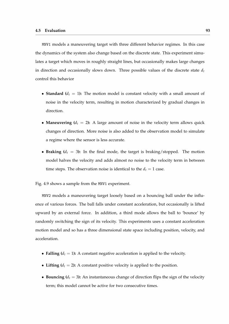
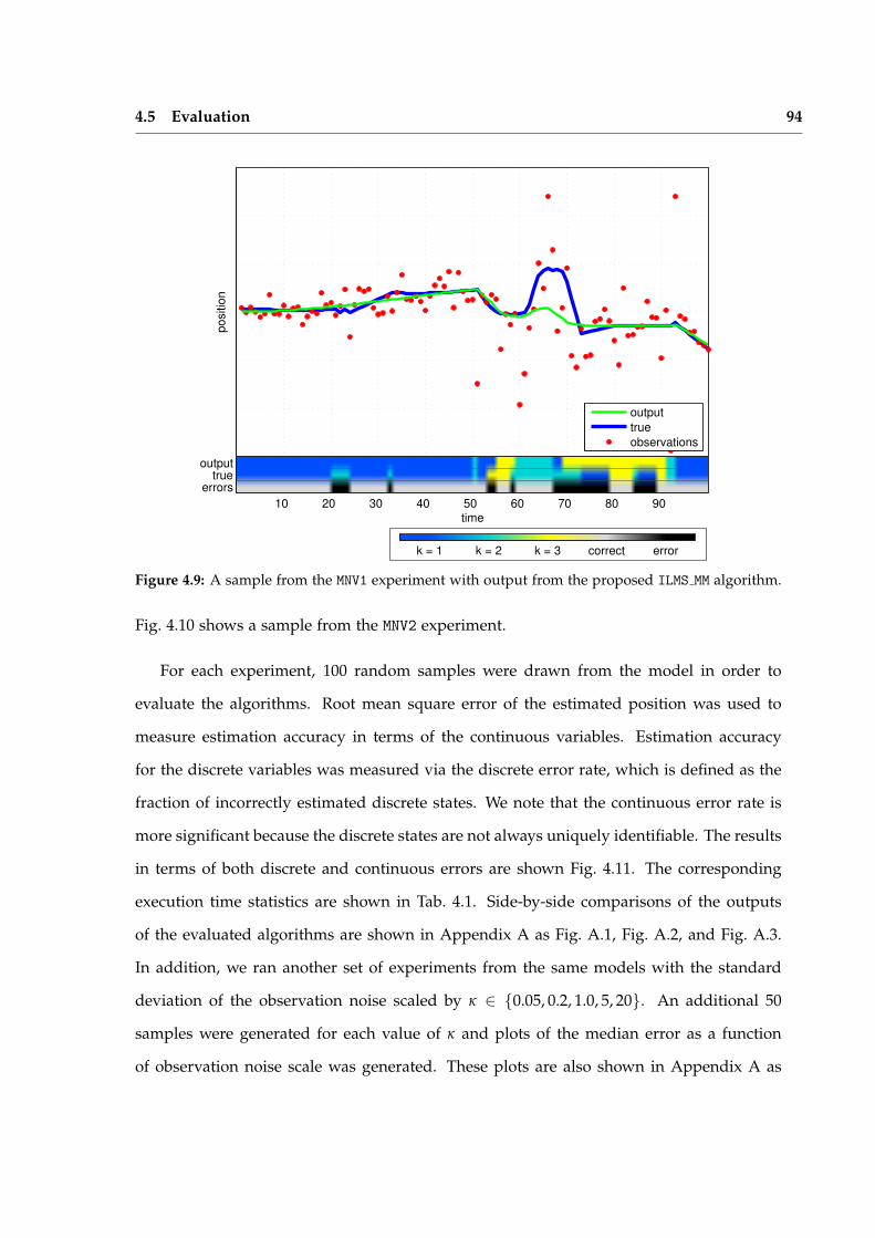
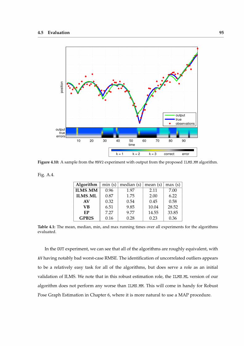
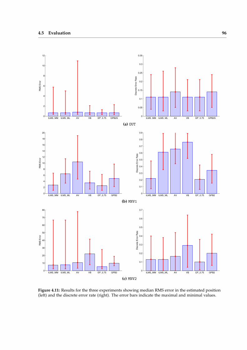
Iterative Local Model Selection for Tracking and Mapping Aleksandr V. Segal St Anne’s College Active Vision Group Department of Engineering Science University of Oxford Michaelmas Term 2014 This thesis is submitted to the Department of Engineering Science, University of Oxford, for the degree of Doctor of Philosophy. This thesis is entirely my own work, and, except where otherwise indicated, describes my own research.
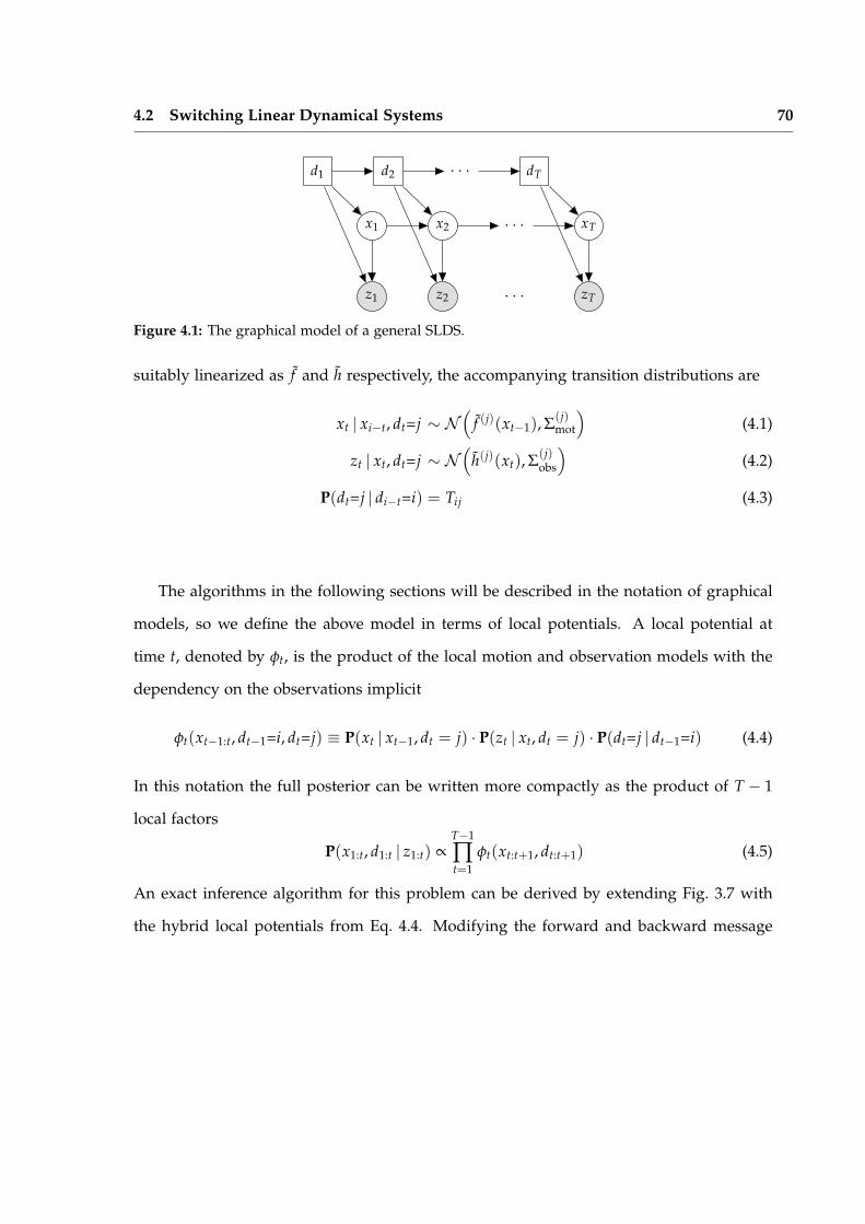
Transcript
Iterative Local Model Selectionfor Tracking and Mapping
Aleksandr V. SegalSt Anne’s College
Active Vision GroupDepartment of Engineering Science
University of Oxford
Michaelmas Term 2014
This thesis is submitted to the Department of Engineering Science, University of Oxford,for the degree of Doctor of Philosophy. This thesis is entirely my own work, and, except
where otherwise indicated, describes my own research.
Aleksandr V. Segal Doctor of PhilosophySt Anne’s College Michaelmas Term 2014
Iterative Local Model Selectionfor Tracking and Mapping
Abstract
The past decade has seen great progress in research on large scale mapping and percep-tion in static environments. Real world perception requires handling uncertain situationswith multiple possible interpretations: e.g. changing appearances, dynamic objects, andvarying motion models. These aspects of perception have been largely avoided throughthe use of heuristics and preprocessing. This thesis is motivated by the challenge of includ-ing discrete reasoning directly into the estimation process.
We approach the problem by using Conditional Linear Gaussian Networks (CLGNs) asa generalization of least-squares estimation which allows the inclusion of discrete modelselection variables. CLGNs are a powerful framework for modeling sparse multi-modalinference problems, but are difficult to solve efficiently. We propose the Iterative LocalModel Selection (ILMS) algorithm as a general approximation strategy specifically gearedtowards the large scale problems encountered in tracking and mapping.
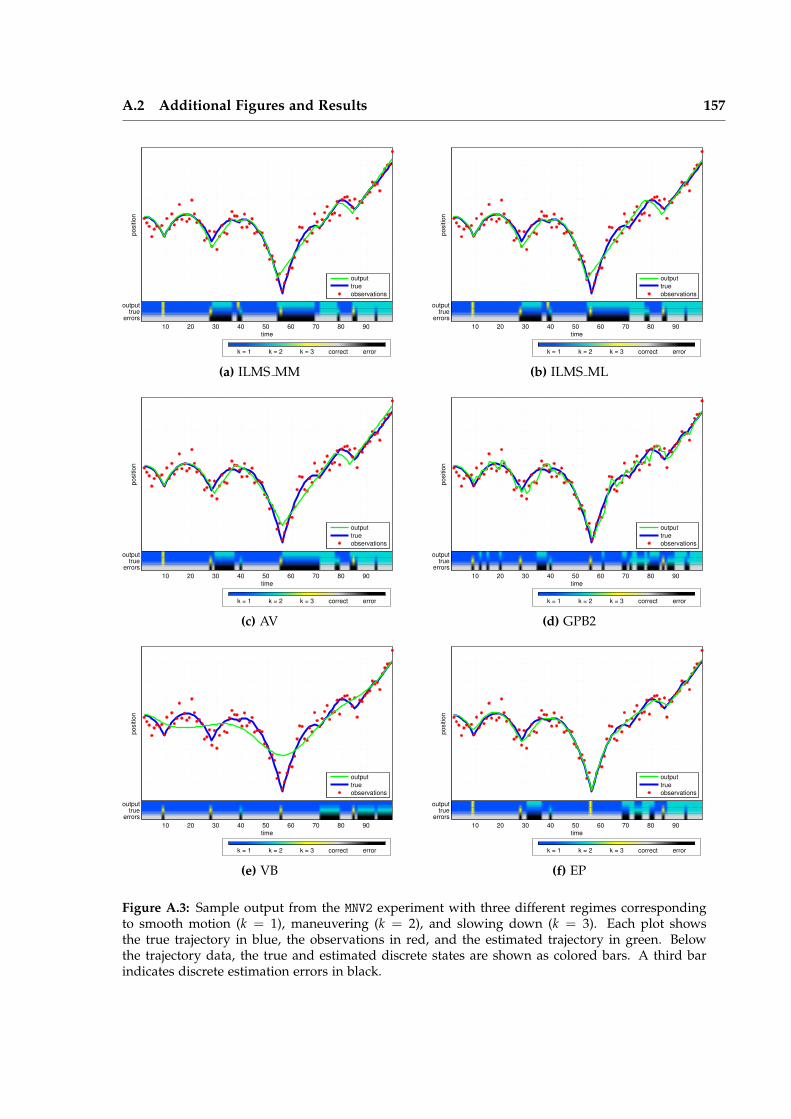
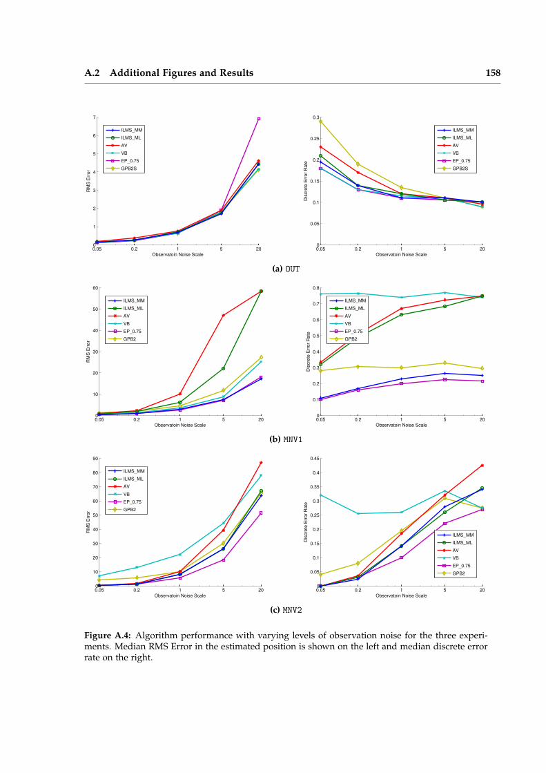
Chapter 4 introduces the ILMS algorithm and compares its performance to traditionalapproximate inference techniques for Switching Linear Dynamical Systems (SLDSs). Theseevaluations validate the characteristics of the algorithm which make it particularly attrac-tive for applications in robot perception. Chief among these is reliability of convergence,consistent performance, and a reasonable trade off between accuracy and efficiency.
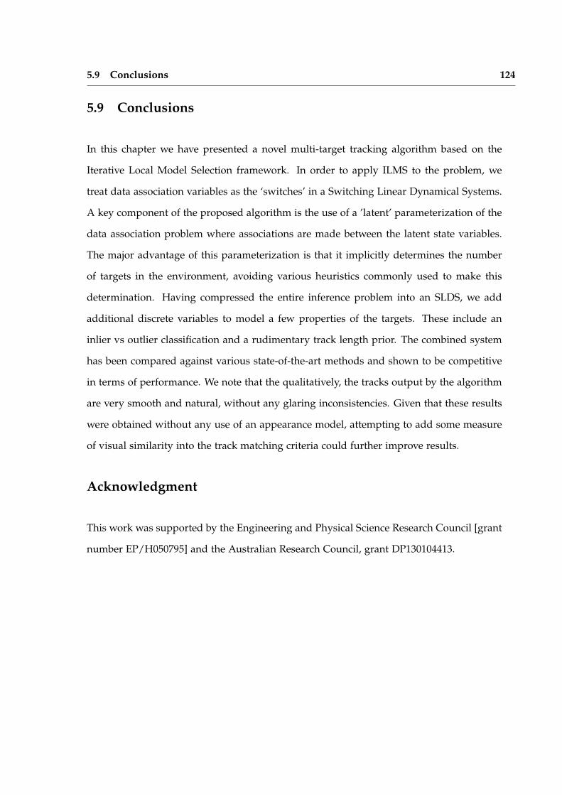
In Chapter 5, we show how the data association problem in multi-target tracking canbe formulated as an SLDS and effectively solved using ILMS. The SLDS formulation al-lows the addition of additional discrete variables which model outliers and clutter in thescene. Evaluations on standard pedestrian tracking sequences demonstrates performancecompetitive with the state of the art.
Chapter 6 applies the ILMS algorithm to robust pose graph estimation. A non-linearCLGN is constructed by introducing outlier indicator variables for all loop closures. Thestandard Gauss-Newton optimization algorithm is modified to use ILMS as an inferencealgorithm in between linearizations. Experiments demonstrate a large improvement overstate-of-the-art robust techniques.
The ILMS strategy presented in this thesis is simple and general, but still works sur-prisingly well. We argue that these properties are encouraging for wider applicability toproblems in robot perception.
I would like to thank my supervisors Ian Reid and David Murray for their guidance
and support in the academic world.
The Active Vision Lab has provided encouragement to push through the hard times
and friends to enjoy the good times. In particular, this thesis would not have been possible
without hours of conversation (and coffee) with Eric Sommerlade and Gabe Sibley.
The majority of the funding for my research was provided by the Engineering and
Physical Sciences Research Council with additional travel support provided by the IEEE
Robotics and Automation Society and St. Anne’s College.
The journey leading up to this dissertation would not have been possible without my
parents and grandparents. There are no words which can describe my appreciation.
To Irina, Thank You. For your patience, for your support, for your untiring spirit.
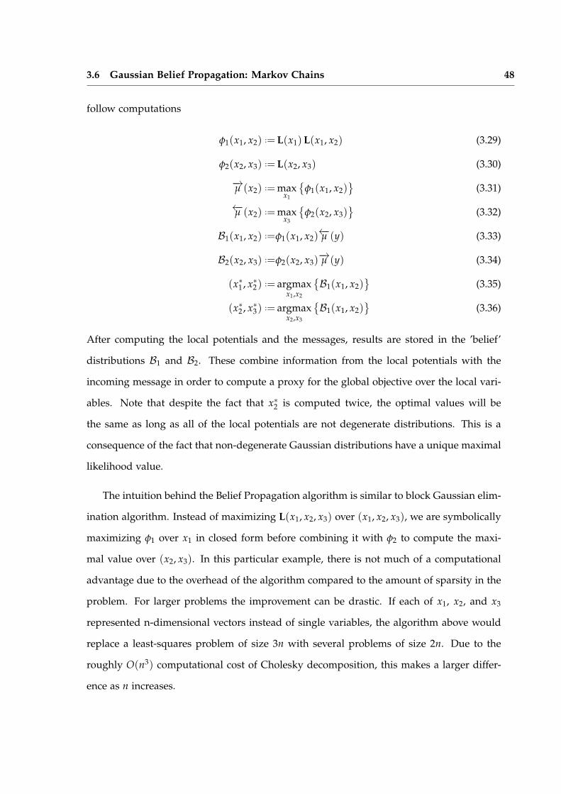
vii
Notation
The following general mathematical notation will be used throughout:
• ||x||Σ =√
x>Σ−1x will denote the Mahalanobis distance/norm
• N (µ, Σ) - multivariate normal distribution with mean µ and covariance Σ.
• N (x ; µ, Σ) - multivariate normal density at point x with mean µ and covariance Σ.
• P(A | B) - probability of A given B
• E[A | B] - expectation of A given B
• Cov[A | B] = E[(A− E[A | B])(A− E[A | B])>
∣∣ B]
- covariance operator
• DKL(P(·)‖Q(·)) =∫
x P(x) log(
P(x)Q(x)
)dx represents the KullbackLeibler divergence.
• δy(·) is the Dirac delta and when used in a probability density function denotes a
discrete value/atom;∫
x∈Ω δy(x)dx =
1 y ∈ Ω0 otherwise
• P(x | z) ∝ f (x, z)⇔ P(x | z) = f (x,z)∑x f (x,z)
• f x = f (x) +∇ f (x)(x− x) used to denote linearization of f at x.
• x⊥⊥ y will be used to denote statistical independence. i.e. P(x, y) = P(x)P(y).
• 1(x) = N (x ; 0, ∞) will be used to denote the fully uninformative ‘distribution’ or the
uniform distribution over the domain if the domain is finite. For Gaussian message
passing this is a degenerate normal distribution parameterized by a 0 information
matrix and vector.
viii
Abbreviations
ILMS Iterative Local Model SelectionSLDS Switching Linear Dynamical SystemCLG Conditional Linear GaussianCLGN Conditional Linear Gaussian NetworkBP Belief PropagationKF Kalman FilterEKF Extended Kalman FilterIEKF Iterated Extended Kalman FilterKS Kalman SmootherIKS Iterated Kalman SmootherSWF Sliding Window FilterSLAM Simultaneous Localization and MappingPGM Probabilistic Graphical ModelPDAF Probabilistic Data Association FilterJPDAF Joint Probabilistic Data Association FilterJCBB Joint Compatibility Branch and BoundMCMC Markov Chain Monte CarloMHT Multi-Hypothesis TrackerDP Dynamic ProgrammingILP Integer Linear ProgramLP Linear ProgramMRF Markov Random FieldGRF Gaussian Random FieldMAP Maximum a PosterioriHMM Hidden Markov ModelLDS Linear Dynamical System
ix
Publications from this thesis
• Latent Data Association: Bayesian Model Selection for Multi-target TrackingA V Segal and I D ReidProc Int Conf on Computer Vision Dec 3-6 2013, Sydney, Australia— Presented in Chapter 5
• Hybrid Inference Optimization for Robust Pose Graph EstimationA V Segal and I D ReidProc IEEE/RSJ Int Conf on Intelligent Robots and Systems Sep 14-18, Chicago IL, USA— Presented in Chapter 6
x
1Introduction
1.1 Motivation
Perception of the world is one of the key research topics in AI, Computer Vision, and
Robotics. At it’s core, the goal is to build an internal representation of the external world
using the available sensors. In AI and Robotics, interpretation of the world is a major part
of the perceive-plan-act loop of an intelligent system. In Computer Vision, perception of
the world through cameras is the definition of the field.
A large body of research has focused on the problem of mapping from a moving plat-
form. In the robots community this has taken the form of Simultaneous Localization and
Mapping (SLAM) – the task of building maps from a moving robot. The problem can be
summarized by the following question: given data about the world collected from a mov-
ing platform, how can we solve for the structure (mapping) of the world together with the
motion of the platform (localization)? Recent research has been successful in solving this
problem using a variety of methods optimized for different world models, sensors, and
situations. State of the art SLAM systems can now work in real-time with both laser and
visual sensors, localize the vehicle they’re mounted on, and map novel parts of the environ-
ment accurately and even robustly. There are still many open problems, but the successes in
handling static environments have opened new areas of research going beyond the original
1.1 Motivation 2
problem formulation.
A current state-of-the-art robot is capable of mapping and navigating a mostly static
and constrained environment. Autonomous vehicles are now almost capable of operating
on a public roads, taking care to follow the rules, and avoiding collisions. These systems,
however, still fall short of anything which could be called intelligent decision making. To
be truly autonomous such robotic systems must eventually see the world as more than just
a collection of points and landmarks. This suggests a long term research goal of richer
mapping and tracking algorithms which incorporate semantic understanding.
In the short term, the field of robot perception is filled with practical difficulties which
require some form of discrete reasoning about the world. The classic examples are data as-
sociation and outlier rejection, two problems which have plagued researchers for decades.
In this case the discrete reasoning is often a nuisance to be circumvented in order to es-
timate the robot pose and map. In other situations, the discrete aspects are the primary
objects of interest and cannot be avoided. Object detection and tracking is one example
where the discrete label is in fact one of the things we would like to know. More expressive
discrete models could, for instance, use knowledge of the typical motions of people, cars,
and bicycles to predict where they are likely to be in the future. These examples suggest
the need for a perception system which can choose among various models to better explain
the world.
The research presented in this dissertation is motivated by these higher level aspects of
the mapping problem. The goal is to incorporate discrete decision making as a first class
component of the perception pipeline rather than on the periphery. We accomplish this by
incorporating discrete variables into the traditionally continuous estimation problems used
for perception. For the remainder of the thesis, we will refer to this strategy as a hybrid
discrete-continuous inference approach or equivalently as model selection.
1.2 Approach 3
1.2 Approach
We propose the use of Switching Linear Dynamical Systems (SLDS) and Conditional Lin-
ear Gaussian Networks (CLGN) as a modeling framework for perception. The SLDS is a
fusion of a discrete Hidden Markov Model (HMM) and a continuous Linear Dynamical
System (LDS). The discrete HMM serves as a model selection prior over the LDS and al-
lows switching between multiple continuous models. CLGNs are a generalization of the
same principle to a broader class of graphical models. The CLGN is the fusion of a discrete
and continuous graphical model in which the discrete layer again switches between various
continuous models.
The SLDS and CLGN are not novel representations, but have received limited practi-
cal attention partly due to the difficulties of inference in these models. In this thesis we
introduce the Iterative Local Model Selection (ILMS) algorithm as an approximate inference
strategy for solving the hybrid inference problems encoded by these models. ILMS is a
modification of the Belief Propagation (BP) algorithm which selects the best local model
as part of the message passing procedure. Although the model selection is greedy, the
choice is iteratively revisited as the algorithm proceeds. The approach is broadly similar
to Expectation Propagation (EP) where a local approximation is iteratively refined. Unlike
Expectation Propagation, however, ILMS has guaranteed convergence and in practice tends
to do so quickly.
We believe the algorithm offers an attractive compromise between speed and accuracy
which is well suited for problems in robot perception. The local nature of the algorithm
makes it a good choice for problems where discrete decision making is local, but the con-
tinuous variables are globally correlated. The applications addressed in this thesis, multi-
target tracking and robust estimation are good examples of such problems. With the Latent
Data Association parameterization of multi-target tracking discussed in Chapter 5, data as-
sociation can be treated as a local discrete estimation problem. The continuous states of
each tracked target across the entire time series are strongly correlated, but the discrete
1.2 Approach 4
data association variables are only related to each other through the chain of continuous
variables representing each target’s state.
Similarly, the robust pose graph estimation application in Chapter 6 is a good use case.
The continuous variables in a pose graph are strongly correlated with each other via the
measurements. The discrete inlier/outlier decisions about each individual loop closure,
however, are not as strongly correlated because outlier loop closures can largely be deter-
mined based on their incompatibility with the odometry data. The compatibility of the loop
closures among themselves is also important, but can be treated as a secondary concern. In
other words, the ‘known’ data associations provide a good enough estimate of the system
state so that additional data can be incorporated piecemeal without explicit consideration
of all possible combinations of inliers and outliers. Many problems in Computer Vision
and Robotics which use heuristics to make decisions about how to incorporate data fall into
this category. These are good candidates for ILMS since the algorithm allows data to be
incorporated locally, but still provides some measure of smoothing and re-interpretation of
previously processed data in light of new evidence.
The proposed approach may not work as well for applications which require too much
coordination between different sets of discrete variables. In such cases the algorithm may
still be applicable if care is taken to structure the problem such that strongly correlated
discrete variables appear in the same local optimization sub-problem. Estimation problems
where distant discrete variables are strongly correlated among themselves, however, are
fundamentally not well suited for this strategy. Structuring these problems to bring the
strongly correlated variables together will remove the advantages of sparsity and make
them intractable.
It is also possible for the algorithm to fail due to its local nature. In the application
to robust pose graph estimation, for example, each loop closure is considered individually
based on its compatibility with the current pose graph estimate. It is possible to imagine an
outlier loop closure which is ‘almost correct’ being interpreted as an inlier and precluding
1.2 Approach 5
the correct (but now incompatible) loop closure from being used. This could result in a
string of off-by-one loop closures being selected due to self-consistent perceptual aliasing.
Despite these limitations, ILMS has significant advantages over standard estimation
techniques — it can handle much richer models in a principled manner while scaling to
realistically sized environments. In the remainder of this section we will describe how
CLGNs can be seen as a generalization of least-squares estimation and outline the ILMS
algorithm.
1.2.1 Continuous State Estimation and Gaussian Random Fields
The typical formulation of state estimation for mapping involves defining variables for
the geometric properties of the map and objectives which define the relationship between
them. The set of objectives and variables define a sparse non-linear least squares problem
which is solved iteratively using the Gauss-Newton algorithm or an equivalent numerical
optimization scheme. In the case of Gauss-Newton, each linearization results in a sparse
quadratic optimization problem which must be solved to compute the next linearization
point. Since the optimization problem may involve tens of thousands of variables, it is
important to take advantage of sparsity. This is typically handled by using one of several
strategies from sparse linear algebra. Alternatively, the quadratic optimization problem can
be interpreted as a Gaussian Random Field (GRF). In this case Belief Propagation can be
used as a sparse inference algorithm for solving the least squares problem. Once we have
switched to the inference perspective, it becomes natural to incorporate model selection by
adding discrete variables to the problem. Generalizing the GRF into a Conditional Linear
Gaussian Network is one way to accomplish this.
1.2.2 Switching Models for Tracking and Mapping
Having added the possibility of discrete modeling into our estimation algorithm, we now
consider what this actually gets us. In this section we will sketch out several possible
1.2 Approach 6
applications of switching models and attempt to demonstrate that they are more powerful
than they may initially appear.
As a simple use case, we can make our estimation robust by using a Mixture-of-
Gaussians observation model with a high variance component for outliers. This corre-
sponds to adding an inlier/outlier indicator variable for each observation. To model streaks
of outliers, such as those caused by occlusions, the indicator variables can be coupled to-
gether with a prior which captures this tendency.
In certain situations, data association can also be treated as a switching model by using
a single ’compound’ discrete variable with a combinatorial number of states (one for each
valid association). Although this may seem impractical, we will show that approximate
inference on such a model is sometimes possible without enumerating all discrete states.
We can also consider behavior modeling of dynamic objects – a more interesting situa-
tion where the discrete variables are a priori correlated. A pedestrian may have a variety of
different behaviors depending on the situation. These would correspond to a set of motion
models describing the motion in each case. Since the behavior at each time is not inde-
pendent, there are correlations between the time-adjacent model selection variables within
each track.
Many other situations could potentially be modeled using switching networks. An
autonomous vehicle may have multiple motion models corresponding to different road
surfaces. An unexpected sensor reading may be interpreted as either a failure of the sensor
itself or a drastic change in the state of the world. Each of these possibilities corresponds
to a switching model. This perspective turns the problem of discrete reasoning into one of
inference in switching models.
1.2.3 Iterative Local Model Selection
The main contribution of this thesis is the Iterative Local Model Selection (ILMS) algorithm
for approximate inference in CLGNs. Iterative Local Model Selection is an approximate
1.2 Approach 7
Belief Propagation algorithm which relies on the observation that many practical model
selection problems are fundamentally local. That is, the discrete variables involved are
primarily correlated with a small neighborhood of other variables.
To explain the algorithm at an intuitive level, consider why the exact Belief Propagation
algorithm becomes intractable for hybrid inference problem. The problem occurs when
the computation of a message requires marginalizing over a discrete variable, resulting in
a Mixture-of-Gaussian message. ILMS avoids this situation by locally picking the ’best’
value for the discrete variable and computing the outgoing message conditioned on this
value. Unlike the standard Belief Propagation algorithm, ILMS no longer converges after a
single upward and downward pass through the clique tree and so requires multiple rounds
of message passing to achieve convergence. The algorithm is ‘local’ because only a local
neighborhood of discrete variables is considered during each message computation. We
refer to the algorithm as ‘iterative’ because the local model selection is revisited multiple
times until the algorithm converges to a consistent solution.
ILMS performs a local search through the discrete space and can be thought of as a
very specific variant of block coordinate ascent where each block contains a small set of
discrete variables together with all continuous variables. The intuition can be illustrated
by a hypothetical linear least-squares problem with outliers. In this problem we want
to estimate the mean of a single variable with two possible models for each observation.
A single binary variable is associated with each observation to indicate the outliers. For a
particular indicator di, we hold the others fixed and pick the best value for di by solving the
least squares problems correspond to the two possible values di = 0 and di = 1. ILMS cycles
through all of the indicator variables updating them in this manner one by one. Cycling in
a particular order and using message passing allows the algorithm to avoid recomputing
the least-squares solution multiple times by updating previous solutions instead of starting
from scratch.
1.3 Contributions 8
1.3 Contributions
The novel contributions of this thesis consist of the ILMS inference algorithm and two
practical applications. The algorithm itself is presented in in Chapter 4 in the context
Switching Linear Dynamical Systems. We formally prove the convergence of the algorithm
and demonstrate its advantages compared to existing approximate inference methods. This
initial evaluation is conducted on a set of synthetic tracking problems where exact ground
truth is known.
In Chapter 5, we show how ILMS can be used for multi-target tracking. The resulting
Latent Data Association algorithm is an approach to multi-target tracking which recasts data
association as an SLDS. For this application, ILMS is used to infer both data associations
and some discrete properties of the individual targets. We include target-specific discrete
states to model track termination, outlier trajectories, and missing observations. Evalua-
tions are performed on real-world data where Latent Data Association is shown to match
state-of-the-art performance as of publication in 2013.
Chapter 6 introduces an application of ILMS for Robust Pose Graph SLAM. We ex-
plicitly introduce discrete variables to model outlier loop closure constraints in the graph,
so that ILMS can infer when an appearance based loop closure detector may have failed.
Because pose graphs are not linear chains of variables, we use a Conditional Linear Gaus-
sian Network model to represent the resulting hybrid inference problem. This requires a
generalization of the ILMS algorithm to clique tree structured models which is possible
due to a novel message passing order. Because pose graph estimation is a non-linear es-
timation problem, we present a variant of the Gauss-Newton algorithm which uses ILMS
instead of a least-squares solver in the inner loop. The resulting Hybrid Inference Optimiza-
tion algorithm demonstrates state-of-the-art performance on publicly available datasets as
of publication in 2014. We note that we were able to either match or beat the state-of-the-
art in both of the presented applications despite using a much more general approach than
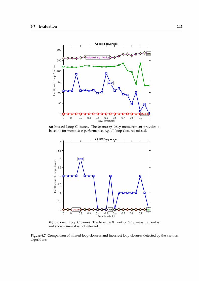
used by competing problem-specific algorithms. Fig. 1.1 highlights results from the two
1.4 Overview 9
applications.
(a) Chapter 5: Multi-Target Tracking.
kitti_02, Ours
X
Y
kitti_02, groundtruth
X
Y
(b) Chapter 6: Robust Pose Graph Estimation.
Figure 1.1: Illustration of results on tracking and mapping applications.
1.4 Overview
The thesis is divided into seven chapters. The following two chapters will cover previous
work in the field and introduce relevant background material as well as the notation which
will be used in the remainder of the thesis. Following these, we will present novel research
in chapters 4-6. The final chapter will draw conclusions and present topics of interest for
future work. The following list summarizes each chapter:
1.4 Overview 10
• Chapter 1 consists of this introduction.
• Chapter 2 outlines related work
• Chapter 3 reviews background material on Non-linear Optimization, Sparse Estima-
tion, Probabilistic Graphical Models, and Gaussian Belief Propagation.
• Chapter 4 introduces the Iterative Local Model Selection (ILMS) algorithm from a
theoretical perspective. This chapter also validates the algorithm on several synthetic
problems.
• Chapter 5 applies the ILMS algorithm to the problem of multi-target tracking from a
stationary platform.
• Chapter 6 applies a generalization of the algorithm to robust pose graph SLAM.
• Chapter 7 draws conclusions from the research conducted and outlines possible av-
enues for future work.
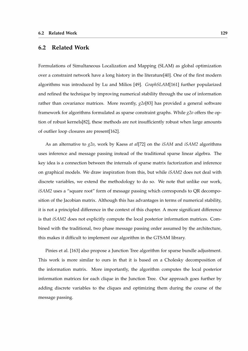
2Related Work
Before introducing novel research, we will start by reviewing the overall progression of
the field. The more specific recent work will be presented in the chapters where it is
most relevant. Two areas of previous work are directly related to this thesis. The first,
Multi-Target Tracking, focuses on tracking moving objects from a static reference frame.
The second, SLAM, deals with tracking a moving sensor platform through an unknown
environment. Although today these are different communities, both fields historically trace
their origins to seminal work on state estimation from the 1960s. In both cases, discrete
variables and various forms of model selection have play an important and challenging role.
In multi-target tracking, the fundamental difficulty is associating observations with targets
and estimating the number of targets in the environment. In the classic SLAM formulation,
data association is often simpler since we are not concerned with a changing environment,
but is nonetheless challenging. We take a unified view of SLAM and multi-target tracking
as sparse state estimation problems with discrete model selection components. Given this
perspective, it is natural to review the background in both of these areas as well as their
connections, before considering a framework for model selection. To this end, we begin by
reviewing the early literature on state estimation, followed by multi-target tracking and the
history of the SLAM problem in Robotics.
2.1 State Estimation and Dynamical Systems 12
2.1 State Estimation and Dynamical Systems
Modern state estimation in dynamical systems was pioneered in the late 1950s and early
1960s for tracking missiles and orbiting satellites. The original problem formulation con-
sisted of a target being tracked and a series of noisy observations of that target. Given a
motion model of the target and a sensor model for the observations, the goal is to estimate
the true motion. The state of the system at time t is represented by the state vector xt.
Observations are denoted zt and a continuous Hidden Markov Model (HMM) is used as the
system model.
The Kalman Filter (KF) [5] was the first practical and real-time estimation algorithm ca-
pable of effectively tracking these targets. The key insight of the KF was that all information
about the past history of observations can be captured by the current state estimate com-
bined with its uncertainty. While Kalman’s original work was presented using different
notation, with modern understanding the Kalman filter can be seen as the simplest case of
a Bayes filter[6, 7]. The KF at time t consists of a Gaussian distribution over xt conditioned
on all previous observations.
P(xt | z1:t) = N(xt ; µxt , Σxt
)(2.1)
At time t + 1, the filter can be updated to include the measurement zt+1 using update
equations based on Bayes’ rule
P(xt+1 | z1:t) =∫
P(xt+1 | xt)P(xt | z1:t)dxt (2.2)
P(xt+1 | z1:t+1) =P(xt+1 | z1:t)P(zt+1 | xt+1)∫
P(xt+1 | z1:t)P(zt+1 | xt+1)dxt+1(2.3)
If both the motion and observation models are linear with Gaussian noise, these updates
can be computed exactly in closed form.
Other variants of the KF algorithm were quickly discovered in the following decade.
Better numerical stability was observed by using the square root covariance matrix Σ =
Σ12 Σ
12>
[8, 9] or alternatively the square root information matrix Σ−1 = I12 I
12>
[10].
2.1 State Estimation and Dynamical Systems 13
The smoothing problem can be defined as the use of observations from t > t0 in order
to compute an estimate of the system state at t0 [11]. Unlike the filtering problem, where
we are maintaining a running estimate of the posterior P(xt | z1:t), in smoothing we are
attempting to estimate P(xt | z1:T) where T > t is some time in the future. Early work on
state estimation also discovered efficient algorithms for performing this task [12, 13]. The
Kalman Smoother (KS) algorithm is based on running two separate filters, one forward and
one backward in time. At any given time, the forward and backward filter estimates can be
combined to generate the optimal maximal likelihood estimate conditioned on both past
and future observations. This algorithm and its generalizations are closely related to sparse
non-linear estimation problems and inference in graphical models.
Kalman’s initial work on linear systems was quickly followed by extensions to non-
linear systems via the Extended Kalman Filter (EKF) [14, 15]. In this case the motion and
observation models contain a non-linear mean function plus Gaussian noise.
P(xt+1 | xt) = N (xt+1 ; f (xt), Σmot) (2.4)
P(zt | xt) = N (zt ; h(xt), Σobs) (2.5)
The EKF is a simple extension of the Kalman filter where the non-linear functions f and h
are linearized at the estimated system state prior to performing the updates in Eq. 2.2 and
Eq. 2.3. In the following set of EKF equations, we use xt to denote the state estimate, and
P, E to denote the approximate linearized distributions and expectations respectively. The
linearized functions are represented by f and h. Given the previous state estimate xt,
Improved accuracy can be achieved by iteratively re-linearizing; this version is known as
the Iterated Extended Kalman Filter (IEKF) and has been applied since at least the 1970s [11].
Bell and Cathey [16] demonstrate that the IEKF is equivalent to linearizing the system after
using the Gauss-Newton algorithm to obtain a local MAP estimate of xt+1
P(xt+1 | xt) = N(xt+1 ; f xt(xt), Σmot
)(2.12)
xt+1 = argmaxxt+1
P(zt+1 | xt+1) P(xt+1 | xt) P(xt | z1:t)
(2.13)
P(zt+1 | xt+1) = N(zt+1 ; hxt+1(xt+1), Σobs
)(2.14)
For the Iterated Kalman Smoother (EKS), a similar equivalence can be made to Gauss-Newton
applied to the full system state vector[17]
x1:t = argmaxx1:t
P(z1 | x1)P(x1) ∏
t=2,...,TP(zt | xt)P(xt | xt−1)
(2.15)
Bell [17] demonstrate that the EKS can be thought of as a sparse decomposition of the global
least squares problem via the Matrix Inversion Lemma. Bertsekas [18] show an equivalence
to incremental least squares and provide a proof of convergence subject to some constraints
on the step size.
More recently the Unscented Transform [19, 20] has been proposed as an alternative to
the linearization in the EKF. The resulting algorithm, referred to as the Unscented Kalman
Filter (UTF), is based on representing the distribution P(xt|z1:t) as a deterministic set of
weighted sample points
Punscented(xt | z1:t) = ∑i
wti · δXti(xt) (2.16)
such that the sample mean and covariance match the target distribution. Instead of lin-
earizing the motion and observations models, the functions ft and ht are applied directly
to the sample points to generate a transformed set of points
Yti = f (Xti) (2.17)
The effect of f on the distribution can be estimated by computing the weighted mean
and covariance of the transformed points. Iterated versions of the UKF have also been
explored [21].
2.1 State Estimation and Dynamical Systems 15
The need to deal with discrete variables and model selection was also recognized early
in the field. In order to deal with an unknown system model, Magill [22] introduced
what has become known as the Multiple Model (MM) approach[11]. MM runs multiple
independent KFs in parallel using the same input data, each with a separate system model.
At each point in time, the output of the MM filter is a linear combination of the filtered
estimates from the bank of filters. The process is effectively being modeled as a mixture
of several independent linear Gaussian models. Crucially, the MM filter does not model a
switching process; it assumes there is a single linear model which explains the data, but we
are are not sure which model it is.
Ackerson and Fu [23] appear to be the first to propose a switching filter which explicitly
models transitions between different discrete states. They propose a KF operating in a set
of different noise environments. A discrete Markov chain models which environment the
system is in at any given time. Each environment corresponds to different noise parameters
in the motion and observation models.
kt ∈ 1, . . . , K (2.18)
P(kt+1 = i | kt = j) = pij (2.19)
P(xt+1 | xt, kt+1 = i) = N(
xt+1 ; ft(xt), Σ(i)mot
)(2.20)
P(zt | xt, kt = i) = N(
zt ; ht(xt), Σ(i)obs
)(2.21)
They observe that optimal filtering is not feasible in such a system because the true repre-
sentation for the posterior P(xt|z1:t) is a mixture with Kt components. An approximation is
proposed where the filtering state is represented by a single Gaussian distribution. Tugnait
[24] present a survey of approximate algorithms for such Switching Linear Dynamical Sys-
tems (SLDS) where the process parameters change according to a discrete Markov process.
They note several approximation schemes similar to Ackerson and Fu [23] which had been
proposed up to that point in time.
Blom [25] introduced the Interacting Multiple Model (IMM) filtering approach as an ex-
tension of the MM filter. This approach is similar in spirit to Ackerson and Fu [23]. Instead
2.2 Tracking 16
of approximating P(xt | z1:t) as a single Gaussian, however, the posterior is approximated
as a mixture of Gaussians over the single discrete variable kt
∑i
P(xt | kt = i, z1:t) P(kt = i | z1:t) ≈∑k1:t
P(xt, k1:t | z1:t)P(k1:t | z1:t) (2.22)
2.2 Tracking
Tracking is a special case of state estimation, but with the additional difficulty of data
association, cluttered ’false-alarm’ sensor readings, and multiple targets. Many of these
difficulties are identical to those arising in the SLAM literature. Traditional approaches
to multi-target tracking were pioneered assuming point-like targets such as radar returns.
Most of these approaches are progressive variations and generalizations of single target
tracking in a cluttered environment.
In a tracking problem, there are typically multiple measurements recorded at each t,
denoted by zti for i = 1, . . . , Mt, which must be associated with the correct targets. Even if
there is only one target, outlier measurements must still be filtered out and ignored.
In the simplest case gating can be used to determine if a candidate measurement orig-
inated from the target being tracked [26]. Given the expected observation zt+1 and its
covariance Σzt+1 ,
zt+1 = E[zt+1 | z1:t] =∫
z · P(zt+1 | xt+1)P(xt+1 | xt)P(xt | z1:t)dz (2.23)
Σzt+1 = Cov[zt+1 | z1:t] (2.24)
each measurement in the new set of observations zt+1,i is considered valid if it passes a
chi-squared test
(zt+1,i − zt+1)>Σ−1
zt+1(zt+1 − zt+1,i) ≤ τ (2.25)
where τ is a chosen based on the desired confidence level and the χ2 distribution. The
valid measurement which is closest to the predicted observation is incorporated into the
filter.
2.2 Tracking 17
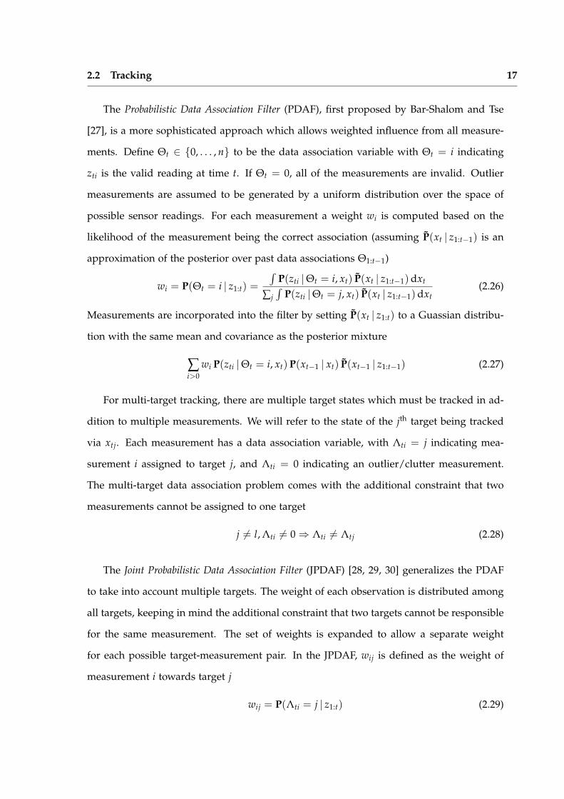
The Probabilistic Data Association Filter (PDAF), first proposed by Bar-Shalom and Tse
[27], is a more sophisticated approach which allows weighted influence from all measure-
ments. Define Θt ∈ 0, . . . , n to be the data association variable with Θt = i indicating
zti is the valid reading at time t. If Θt = 0, all of the measurements are invalid. Outlier
measurements are assumed to be generated by a uniform distribution over the space of
possible sensor readings. For each measurement a weight wi is computed based on the
likelihood of the measurement being the correct association (assuming P(xt | z1:t−1) is an
approximation of the posterior over past data associations Θ1:t−1)
wi = P(Θt = i | z1:t) =
∫P(zti |Θt = i, xt) P(xt | z1:t−1)dxt
∑j∫
P(zti |Θt = j, xt) P(xt | z1:t−1)dxt(2.26)
Measurements are incorporated into the filter by setting P(xt | z1:t) to a Guassian distribu-
tion with the same mean and covariance as the posterior mixture
∑i>0
wi P(zti |Θt = i, xt)P(xt−1 | xt) P(xt−1 | z1:t−1) (2.27)
For multi-target tracking, there are multiple target states which must be tracked in ad-
dition to multiple measurements. We will refer to the state of the jth target being tracked
via xtj. Each measurement has a data association variable, with Λti = j indicating mea-
surement i assigned to target j, and Λti = 0 indicating an outlier/clutter measurement.
The multi-target data association problem comes with the additional constraint that two
measurements cannot be assigned to one target
j 6= l, Λti 6= 0⇒ Λti 6= Λtj (2.28)
The Joint Probabilistic Data Association Filter (JPDAF) [28, 29, 30] generalizes the PDAF
to take into account multiple targets. The weight of each observation is distributed among
all targets, keeping in mind the additional constraint that two targets cannot be responsible
for the same measurement. The set of weights is expanded to allow a separate weight
for each possible target-measurement pair. In the JPDAF, wij is defined as the weight of
measurement i towards target j
wij = P(Λti = j | z1:t) (2.29)
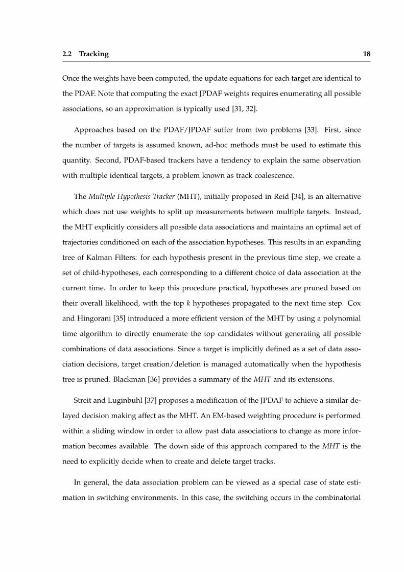
2.2 Tracking 18
Once the weights have been computed, the update equations for each target are identical to
the PDAF. Note that computing the exact JPDAF weights requires enumerating all possible
associations, so an approximation is typically used [31, 32].
Approaches based on the PDAF/JPDAF suffer from two problems [33]. First, since
the number of targets is assumed known, ad-hoc methods must be used to estimate this
quantity. Second, PDAF-based trackers have a tendency to explain the same observation
with multiple identical targets, a problem known as track coalescence.
The Multiple Hypothesis Tracker (MHT), initially proposed in Reid [34], is an alternative
which does not use weights to split up measurements between multiple targets. Instead,
the MHT explicitly considers all possible data associations and maintains an optimal set of
trajectories conditioned on each of the association hypotheses. This results in an expanding
tree of Kalman Filters: for each hypothesis present in the previous time step, we create a
set of child-hypotheses, each corresponding to a different choice of data association at the
current time. In order to keep this procedure practical, hypotheses are pruned based on
their overall likelihood, with the top k hypotheses propagated to the next time step. Cox
and Hingorani [35] introduced a more efficient version of the MHT by using a polynomial
time algorithm to directly enumerate the top candidates without generating all possible
combinations of data associations. Since a target is implicitly defined as a set of data asso-
ciation decisions, target creation/deletion is managed automatically when the hypothesis
tree is pruned. Blackman [36] provides a summary of the MHT and its extensions.
Streit and Luginbuhl [37] proposes a modification of the JPDAF to achieve a similar de-
layed decision making affect as the MHT. An EM-based weighting procedure is performed
within a sliding window in order to allow past data associations to change as more infor-
mation becomes available. The down side of this approach compared to the MHT is the
need to explicitly decide when to create and delete target tracks.
In general, the data association problem can be viewed as a special case of state esti-
mation in switching environments. In this case, the switching occurs in the combinatorial
2.3 Mapping 19
space of all possible data associations. Just as in the case of switching dynamical systems,
the possible data associations create a mixture model posterior. Many of the above data
associations algorithms amount to various approximations of this mixture.
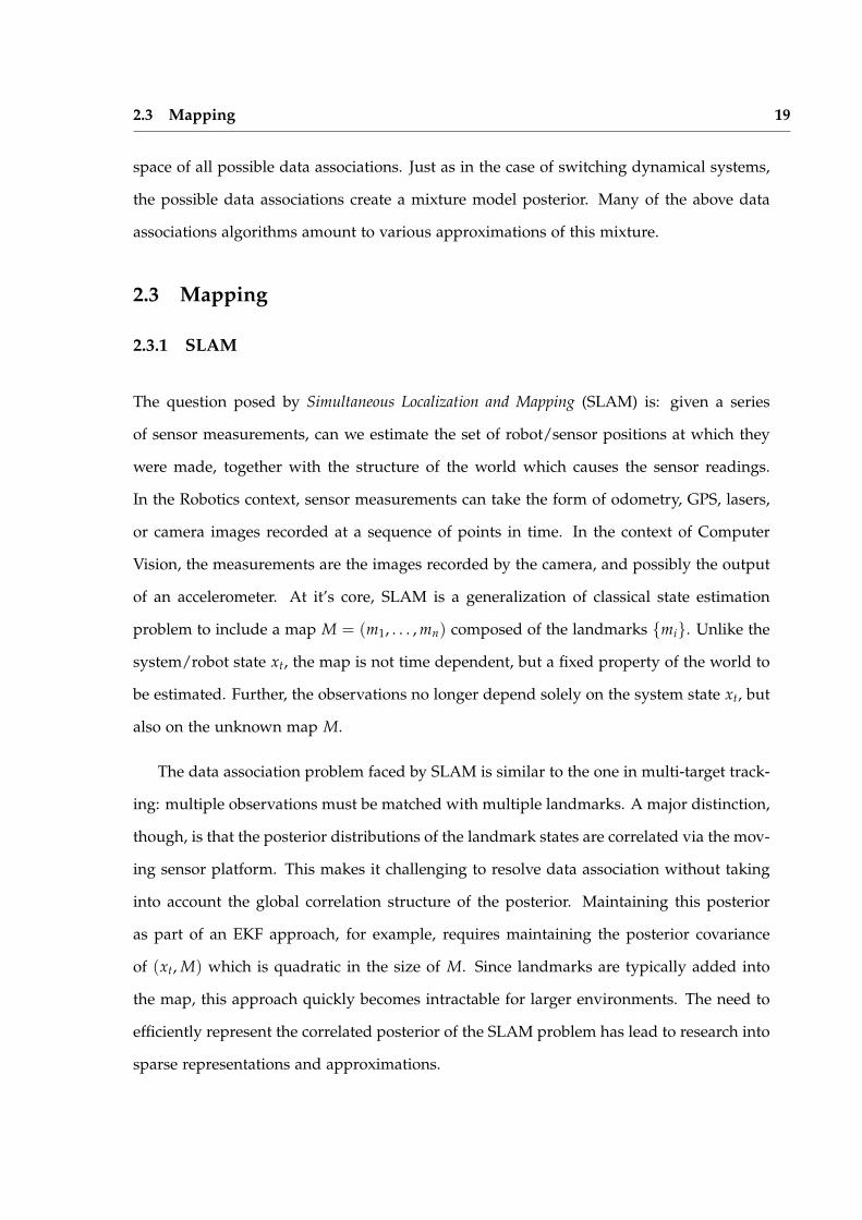
2.3 Mapping
2.3.1 SLAM
The question posed by Simultaneous Localization and Mapping (SLAM) is: given a series
of sensor measurements, can we estimate the set of robot/sensor positions at which they
were made, together with the structure of the world which causes the sensor readings.
In the Robotics context, sensor measurements can take the form of odometry, GPS, lasers,
or camera images recorded at a sequence of points in time. In the context of Computer
Vision, the measurements are the images recorded by the camera, and possibly the output
of an accelerometer. At it’s core, SLAM is a generalization of classical state estimation
problem to include a map M = (m1, . . . , mn) composed of the landmarks mi. Unlike the
system/robot state xt, the map is not time dependent, but a fixed property of the world to
be estimated. Further, the observations no longer depend solely on the system state xt, but
also on the unknown map M.
The data association problem faced by SLAM is similar to the one in multi-target track-
ing: multiple observations must be matched with multiple landmarks. A major distinction,
though, is that the posterior distributions of the landmark states are correlated via the mov-
ing sensor platform. This makes it challenging to resolve data association without taking
into account the global correlation structure of the posterior. Maintaining this posterior
as part of an EKF approach, for example, requires maintaining the posterior covariance
of (xt, M) which is quadratic in the size of M. Since landmarks are typically added into
the map, this approach quickly becomes intractable for larger environments. The need to
efficiently represent the correlated posterior of the SLAM problem has lead to research into
sparse representations and approximations.
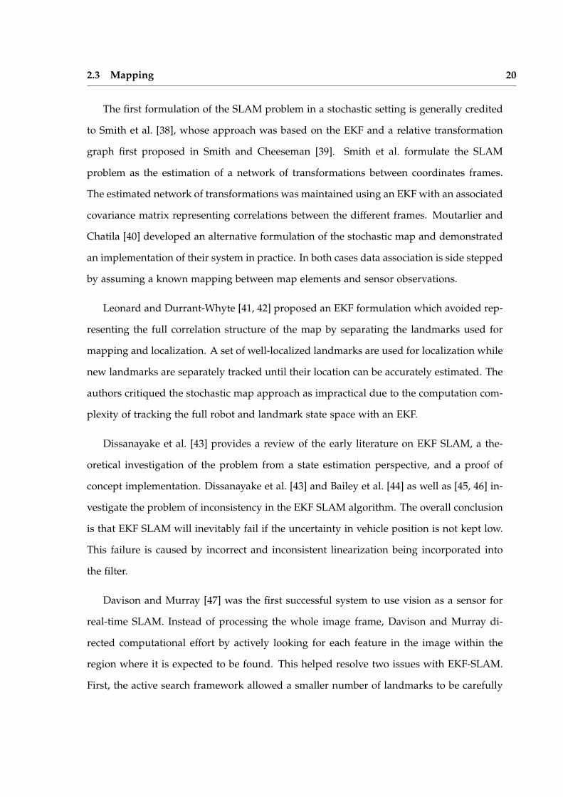
2.3 Mapping 20
The first formulation of the SLAM problem in a stochastic setting is generally credited
to Smith et al. [38], whose approach was based on the EKF and a relative transformation
graph first proposed in Smith and Cheeseman [39]. Smith et al. formulate the SLAM
problem as the estimation of a network of transformations between coordinates frames.
The estimated network of transformations was maintained using an EKF with an associated
covariance matrix representing correlations between the different frames. Moutarlier and
Chatila [40] developed an alternative formulation of the stochastic map and demonstrated
an implementation of their system in practice. In both cases data association is side stepped
by assuming a known mapping between map elements and sensor observations.
Leonard and Durrant-Whyte [41, 42] proposed an EKF formulation which avoided rep-
resenting the full correlation structure of the map by separating the landmarks used for
mapping and localization. A set of well-localized landmarks are used for localization while
new landmarks are separately tracked until their location can be accurately estimated. The
authors critiqued the stochastic map approach as impractical due to the computation com-
plexity of tracking the full robot and landmark state space with an EKF.
Dissanayake et al. [43] provides a review of the early literature on EKF SLAM, a the-
oretical investigation of the problem from a state estimation perspective, and a proof of
concept implementation. Dissanayake et al. [43] and Bailey et al. [44] as well as [45, 46] in-
vestigate the problem of inconsistency in the EKF SLAM algorithm. The overall conclusion
is that EKF SLAM will inevitably fail if the uncertainty in vehicle position is not kept low.
This failure is caused by incorrect and inconsistent linearization being incorporated into
the filter.
Davison and Murray [47] was the first successful system to use vision as a sensor for
real-time SLAM. Instead of processing the whole image frame, Davison and Murray di-
rected computational effort by actively looking for each feature in the image within the
region where it is expected to be found. This helped resolve two issues with EKF-SLAM.
First, the active search framework allowed a smaller number of landmarks to be carefully
2.3 Mapping 21
tracked, rather then extracting large numbers of features and initializing a large number of
new landmarks at each frame. Second, since EKF-SLAM kept track of landmark position
uncertainty, projecting the current uncertainty ellipse onto the image plane placed a bound
on where the landmark was likely to be observed. By only searching within these bounds,
efficiency was greatly increased.
[48] investigates a distributed version of SLAM and suggests the use of the Information
Filter over the more standard Kalman Filter. The information parameterization allows
incorporating novel information by simply adding constraints to the representation without
performing any matrix inversions. This approach is particularly useful for multi-robot
problems, but has advantages for standard SLAM as well.
An alternative formulation of SLAM, known as pose graph estimation, was proposed
by Lu and Milios [49]. The pose graph approach removes landmarks from the map entirely
and treats the problem as one of estimating a network of robot positions. Constraints
between poses can be generated by using scan matching [50] to align the observed sensor
readings. The network of constraints, referred to as a pose graph, is directly optimized.
In contrast to EKF SLAM, where only the most recent pose is tracked, pose graph SLAM
updates the full trajectory of the robot and so avoids permanently incorporating inaccurate
linearizations. The Sparse Extended Information Filter (SEIF) [51] combines the advantages
of the Information Filter parameterization with the pose graph formulation of Lu and
Milios [49]. Nuchter et al. [52] extends the Graph SLAM approach to 3D environments
by using laser generated pointclouds as input and the Iterative Closest Point (ICP) [50]
algorithm for scan matching.
Montemerlo et al. [53] introduced the FastSLAM algorithm which is based on a com-
bination of sampling and the EKF. The key realization was that conditioning on the robot
trajectory made all of the landmarks conditionally independent. By representing the dis-
tribution over trajectories as a finite set of samples, the locations of the landmarks became
conditionally independent when conditioned on a single trajectory sample. This allowed
2.3 Mapping 22
FastSLAM to avoid the O(n2) running cost of EKF-SLAM at the expense of sampling the
space of trajectories. This approach was extremely successful for robots constrained to a
plane and equipped with range sensors such as laser scanners and sonar. Sim et al. [54]
adapted the FastSLAM approach to a visual setting using a stereo rig and SIFT features
[55].
Davison et al. [56] introduced MonoSLAM, the first real-time monocular SLAM algo-
rithm. Unlike previous work which relied on either accurate odometry estimates, or slow
sensor movement, the algorithm introduced by Davison et al. works on a rapidly moving
hand-held camera without any odometry. An active search procedure similar to Davison
and Murray [47] is used to locate features, and a delayed initialization scheme is used to
help estimate the position of landmarks. Since a monocular camera cannot give a 3D posi-
tion estimate when a feature is first observed, Davison et al. used a collapsed particle filter
to estimate a distribution of possible landmark locations along a ray. When this distribu-
tion is sufficiently close to being Gaussian, the landmark is fully initialized and tracked
with EKF-SLAM.
Eade and Drummond [57] present a monocular FastSLAM as an alternative to EKF-
SLAM. Eade and Drummond combined the top-down active search of [47], with an im-
proved version of the delayed initialized procedure in [56]. The improved initialization
procedure uses an inverse-depth parameterization to sample particles along an initial ray.
Unlike MonoSLAM, the particles are used to estimate camera position even before the
landmark is fully initialized.
2.3.2 Structure from Motion
Structure-from-Motion is a similar, but historically independent estimation technique used
for offline map-building. Unlike research in SLAM, which has focused on providing a
real-time solution to the online version of the problem, SfM has focused on offline map
estimation from a large set of images. This procedure traces its history back to the early
2.3 Mapping 23
19th century roots of Photogrammetry [58], which uses photographs to estimate topography
for map-making. The Photogrammetry community had coined the term bundle adjustment
(in reference to adjusting the bundles of rays going from features to camera planes) to
refer to the process of least squares estimation of these maps based on matching features
between photographs.
A modern understanding of the procedure from the computer vision perspective is pre-
sented in the survey by Triggs et al. [59], as well as Hartley and Zisserman [60]. We will
define Xj as a set of 3D points whose position is unknown. These points will loosely
correspond to the M variable in the SLAM formulation. The points are observed through
a set of cameras, which will be known via their set of projection operators Pi. The appli-
cation of a camera projection operator, Pi, onto a 3D point, Xj, yields a 2D measurement of
that point, xij = Pi(Xj).
Once we are given the set of observations xij, we can define the bundle adjustment
problem as least-squares estimation of all of the camera parameters together with the loca-
tions of the 3D points (landmarks in the SLAM terminology):
argminPi,Xj
(∑i,j||Pi(Xj)− xi
j||2Σ) (2.30)
where || · ||Σ is the L2 norm using Σ as the metric.
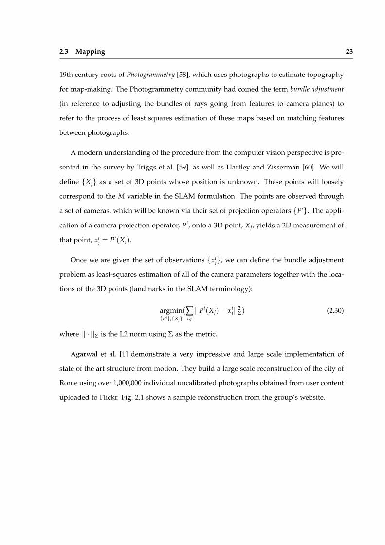
Agarwal et al. [1] demonstrate a very impressive and large scale implementation of
state of the art structure from motion. They build a large scale reconstruction of the city of
Rome using over 1,000,000 individual uncalibrated photographs obtained from user content
uploaded to Flickr. Fig. 2.1 shows a sample reconstruction from the group’s website.
2.4 Sparsity and Decomposition 24
Figure 2.1: A reconstruction of the Colosseum in Rome obtained from Agarwal et al. [1]
2.4 Sparsity and Decomposition
The topic of sparsity and decomposition deals with efficient computational methods which
take advantage of the sparse relationships between variables in problems. Such methods
are required for both mapping and tracking because the full state spaces of these problems
often involves tens of thousands of variables. For tracking problems, the Kalman Filter and
Smoother can be thought of as sparse estimation algorithms. In multi-target tracking, the
fact the each track is represented as an independent Kalman filter is also a form of sparsity.
In the SfM and SLAM communities, a large body of research has targeted efficient de-
compositions of the estimation problem which are applicable to large data sets. The idea
behind this line of research is to partition a large mapping problem into multiple smaller
problems which can be more easily handled. The local maps can then be merged into a
global map estimate. There are two practical advantages to this approach. First, it allows
maps larger than the memory of the computer to be built. Second, the algorithm is more
efficient since it ignores the generally weaker dependencies between distance map features.
Maintaining the full cross covariance between distance landmarks is the main cause of the
quadratic memory footprint of EKF-SLAM. Much like the Sparse Extended Information
Filter (SEIF) [51], we can gain a computational advantage by maintaining these cross cor-
relations only when they are strong. Whereas the SEIF does this by examining individual
entries in the dependency graph for relevance, submapping approaches to SLAM and SfM
take advantage of the natural tendency of distance landmarks to be weekly correlated.
2.4 Sparsity and Decomposition 25
Chong and Kleeman [61] introduced one of the first submapping schemes where local
maps were built up for each region of the environment. Each local map was treated as an
independent mapping problem with a reference frame based on the initial robot position
at the ’start’ of the map. Within each local map, a full covariance estimate of all landmarks
is tracked using EKF SLAM. Landmarks which are not part of the same submap do not
have an explicit representation of their relative covariance stored. Instead, the covariance
between the local reference frames themselves is maintained. Leonard and Feder [62] use
a similar scheme, except with a global reference coordinate the offsets between submaps.
This simplifies finding the appropriate submap for the current robot pose since the loca-
tions of the submaps themselves are stored in a single reference frame.
In Bosse et al. [63] each local submap is stored in its own coordinate system, with a
network of relative transformations between the local frames. This is similar in principle
to the original stochastic map, but here each vertex represents an entire submap rather
than a single map feature. The network of coordinate frames is undirected with loops
allowed. Dijkstra’s algorithm is used on this network to find chains of transformation be-
tween different coordinate frames. The algorithm maintains a set of hypothesis local maps
and tracks the robot in parallel in each of the hypothesis. This avoids relying on a single
local map and allows smooth transitions to different local representations by changing the
active set of hypotheses. Periods of simultaneous tracking within multiple hypotheses are
used to refine the estimated transformations between the corresponding submaps.
Sibley et al. [64], Mei et al. [65] introduce a system based on the natural limit of the
submapping approach of Bosse et al. [63]. In this case each individual robot pose is re-
garded as a separate submap containing only the landmarks which were first observed at
that time. This allows constant time operation since incorporating new observations into
the problem does not effect any variables beyond a relatively small set of poses in the past.
Specifically, adding observations of a landmark induces correlations with all other robot
poses which have observed that landmark though the chain of relative transformations be-
tween these poses. Since all transformations are stored in a relative representation, any
2.4 Sparsity and Decomposition 26
pose not on this chain becomes independent of the new measurements.
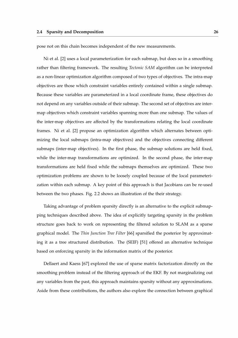
Ni et al. [2] uses a local parameterization for each submap, but does so in a smoothing
rather than filtering framework. The resulting Tectonic SAM algorithm can be interpreted
as a non-linear optimization algorithm composed of two types of objectives. The intra-map
objectives are those which constraint variables entirely contained within a single submap.
Because these variables are parameterized in a local coordinate frame, these objectives do
not depend on any variables outside of their submap. The second set of objectives are inter-
map objectives which constraint variables spanning more than one submap. The values of
the inter-map objectives are affected by the transformations relating the local coordinate
frames. Ni et al. [2] propose an optimization algorithm which alternates between opti-
mizing the local submaps (intra-map objectives) and the objectives connecting different
submaps (inter-map objectives). In the first phase, the submap solutions are held fixed,
while the inter-map transformations are optimized. In the second phase, the inter-map
transformations are held fixed while the submaps themselves are optimized. These two
optimization problems are shown to be loosely coupled because of the local parameteri-
zation within each submap. A key point of this approach is that Jacobians can be re-used
between the two phases. Fig. 2.2 shows an illustration of the their strategy.
Taking advantage of problem sparsity directly is an alternative to the explicit submap-
ping techniques described above. The idea of explicitly targeting sparsity in the problem
structure goes back to work on representing the filtered solution to SLAM as a sparse
graphical model. The Thin Junction Tree Filter [66] sparsified the posterior by approximat-
ing it as a tree structured distribution. The (SEIF) [51] offered an alternative technique
based on enforcing sparsity in the information matrix of the posterior.
Dellaert and Kaess [67] explored the use of sparse matrix factorization directly on the
smoothing problem instead of the filtering approach of the EKF. By not marginalizing out
any variables from the past, this approach maintains sparsity without any approximations.
Aside from these contributions, the authors also explore the connection between graphical
2.4 Sparsity and Decomposition 27
Figure 2.2: A figure from Ni et al. [2] illustrating the submapping procedure and dependenciesbetween variables within the submaps
representations of the mapping problem and sparse matrix factorization. They note that the
column ordering heuristics typically employed by sparse matrix factorization algorithms
are analogous to graph triangulation techniques used in the graphical model community
to construct junction trees. Along these lines Krauthausen et al. [68] investigates the used
of Nested Dissection as a column order scheme and Ni and Dellaert [69] shows how the
Nested Dissection scheme can be used to automatically partition a problem into recursive
submaps.
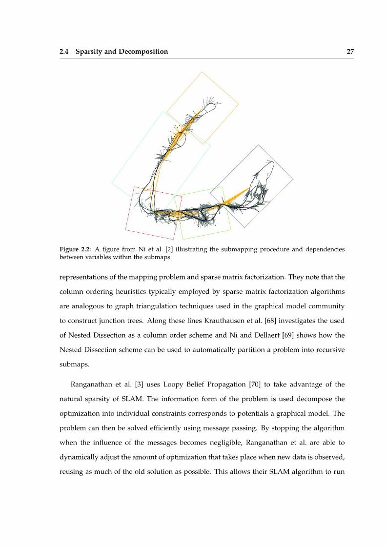
Ranganathan et al. [3] uses Loopy Belief Propagation [70] to take advantage of the
natural sparsity of SLAM. The information form of the problem is used decompose the
optimization into individual constraints corresponds to potentials a graphical model. The
problem can then be solved efficiently using message passing. By stopping the algorithm
when the influence of the messages becomes negligible, Ranganathan et al. are able to
dynamically adjust the amount of optimization that takes place when new data is observed,
reusing as much of the old solution as possible. This allows their SLAM algorithm to run
2.4 Sparsity and Decomposition 28
in O(1) time without loop closure, and in O(n) time when loops closures occur (where n
is the size of the loop).
Figure 2.3: A figure from Ranganathan et al. [3] showing the operation of the algorithm when newinformation is added. Red colored nodes in the graph indicate variables which are being optimized,while yellow nodes are unaffected. When loop closure does not occur (left), only a small windowof variables around the new information is affected. When loop closure happens (right), all of thenodes in the loop are optimized in order to spread out error along the loop as best as possible.
Kaess et al. [71] presents an incremental approach to the smoothing problem based
on the connections between probabilistic graphical models and sparse matrix factorization
presented in Dellaert and Kaess [67]. Kaess et al. [72] builds on this by adding a specialized
data structure referred to as a Bayes Tree. The Bayes Tree allows an online approach to
smoothing with incremental variable re-ordering and linearization. This eliminates the
need for the batch operations required in Kaess et al. [71].
Sliding Window Filters (SWF), introduced to SLAM by Sibley et al. [73], offer a com-
promise between the online approach of filtering and the batch processing used in SfM.
Instead of processing observations one at a time, a limited set of the most recent observa-
tions (those within the sliding window) is processed in batch mode, while all observations
beyond the edge of this window are summarized with a recursively updated state esti-
mate. The filtering disribution of a SWF of length κ is P(xt−κ:t|z1:t). Using such a filter
allows us to improve our estimate of xt−κ using information from the future (zt−κ+1:t). This
2.5 Model Selection 29
idea is particularly interesting when combined with the Iterated EKF, where it allows the
linearization point of the last κ states to be iteratively updated.
Using the result of Bell and Cathey [16], which showed that the Iterated EKF is equiv-
alent to the Gauss-Newton method for non-linear least squares, we can see that adjusting
the value of κ can produce a range of algorithms from bundle-adjustment to the Kalman
Filter. Setting κ = t corresponds to solving the full least squares problem. Setting κ = 1
corresponds to the Iterated EKF. For values in between the two extremes, we are perform-
ing a full optimization over the set of variables xt−κ:t, but marginalizing out xt−κ before we
move on to the next time step.
2.5 Model Selection
Model selection is the primary topic of this dissertation, so in this section we review previ-
ous work from this perspective. Although it is not always explicitly called model selection,
discrete decision making is nonetheless present in much of the previous work on tracking
and mapping. Data association is the main model selection topic of interest and is generally
acknowledged as one of the most challenging aspects of multi-target tracking. A second
area of research has been on maneuvering targets where multiple distinct models are used
to explain the observed behavior of a target. Since previous work on both of these topics
has already been discussed in Section 2.2, this section will focus on mapping.
2.5.1 Mapping and Data Association
Unlike in tracking, data association for mapping problems is easier to circumvent with
heuristics. The goal in the mapping problem is to build a reconstruction of the environment
which can be used to accurately localize the robot or provide a high level map. Since the
goal is not to track every single possible landmark, heuristic algorithms can be used to
choose distinctive features and landmarks which are easily identifiable. This approach is
particularly attractive in visual SLAM and Structure-from-Motion due to the availability of
2.5 Model Selection 30
good feature descriptors such as SIFT [55].
Agarwal et al. [1] uses SIFT to extract distinct image features and computes potential
matches in a second image using an efficient approximate nearest neighbor algorithm.
The candidate matches are then filtered based on a heuristic test and the RANSAC [74]
algorithm is applied to the remaining matches in order to enforce geometric consistency
between the two images. This procedure, which has a history in cartography dating to at
least 1981 [74], transforms the data association problem into one of outlier rejection. Once
a large enough list of potential feature matches is computed, RANSAC is used to select a
subset of inliers. The result is used as input for an optimization procedure which takes into
account all feature matches to estimate 3D structure and camera locations.
The Visual SLAM algorithm of Davison and Murray [47] uses a combination of gating
and a visual search procedure for data association. The estimated landmark position and
covariance from the current state of the filter are used to physically point the camera in
the direction of the landmark. A 2D search is conducted to find an image patch visually
similar to the original patch used to initiate the landmark. The search is restricted to the
area of the image where the landmark are expected based on the filter covariance. When
a match is found, it is incorporated into the filter as an observation of the landmark. The
MonoSLAM system of Davison et al. [56] uses a similar approach for active feature search,
except without a physically actuated camera.
Pose graph optimization approaches make use of various pre-processing strategies to
establish the graph structure used in the optimization. If visual information is available,
visual similarity can be used to find loop closures [75]. The precise offset between the poses
can be computed using feature matching and RANSAC. With laser data, scan matching
techniques such as the ICP algorithm [50] are used to compute offsets between poses in the
graph.
Because laser and sonar based sensor do not provide unique identifying information
about each feature, early SLAM systems based on these sensors used data association
2.5 Model Selection 31
techniques from the tracking literature combined with heuristics to identify features such
as corners. Data association techniques used include gating [41, 42, 31] and MHT [76,
77] based approaches. We note that Cox and Leonard [77] recognized the fundamental
similarity of multi-target tracking and SLAM when viewed from the MHT perspective;
the difference being that SLAM assumes static landmarks whereas multi-target tracking
assumes a static sensor.
Other ideas based on a hypothesis tree similar to the MHT have been suggested in
the literature. The most relevant to this dissertation is the Joint Compatibility Branch and
Bound (JCBB) [78] data association algorithm. JCBB builds a data association hypothesis
tree for each measurement within one time slice. Each individual measurement zti can be
assigned to any of the existing targets and the decision tree of possible assignments defines
an interpretation tree. JCBB applies a branch and bound search procedure to this inter-
pretation tree in order to find a valid assignment hypothesis which maximizes the number
of matches. A hypothesis is considered valid if it passes a multivariate gating criterion
(the joint compatibility test) on all target-measurement pairs present in the hypothesis. By
gating the entire hypothesis rather than individual landmarks, the correlations between
landmark estimates typical in SLAM is taken into account. A procedure similar in spirit is
proposed in Hahnel et al. [79], but in this case the emphasis is on allowing data associations
from the past to be reconsidered.
Algorithms based on Expectation Maximization (EM) provide an efficient alternative
to explicitly considering the tree of all possible model combinations. Under this heading
we consider both true EM algorithms which optimize a variational bound and EM-like al-
gorithms which operate on intuitively similar principles. An MCMC-based algorithm for
data association using EM was proposed for SfM applications in Dellaert et al. [80]. This
is similar to the JPDAF [29], except the full posterior over data associations at each t is
sampled with an MCMC algorithm to obtain the data association weights. Bibby and Reid
[4] use classification EM within a sliding window filter to allow reversible data associa-
tion and model selection between stationary and moving landmarks/targets. The dynamic
2.5 Model Selection 32
environment aspects of this paper are also discussed in the follow subsection. The Switch-
able Constraint [81] algorithm relaxes discrete variables into continuous variables and adds
them directly into the non-linear optimization problem. The resulting optimization prob-
lem consists of weighted objectives of the form w · g(x) which are optimized over both w
and x. This applies mainly to robust estimation problems where down-weighting the objec-
tives can be used to discard outliers. In the same vein, the older robust estimation methods
such as Iteratively Reweighted Least Squares and Huber/Cauchy kernels [82] have also
been applied to mapping [83].
2.5.2 Mapping in Dynamic Environments
Solving the SLAM problem in a non-static environment requires dealing with the possi-
bility of moving objects such as people, cars, or other robots. These challenges have given
rise to many specialized algorithms which can easily be interpreted as instances of model
selection. The most basic strategy is to ignore dynamic objects entirely by treating them as
outliers – this is the choice implicitly made when dynamic elements of the scene are not
considered. A more sophisticated strategy is to treat the two problems as roughly inde-
pendent. For example, Schulz et al. [84], Hahnel et al. [85], Schulz et al. [86] are a series
of results which combine a multi-target tracking system with SLAM to filter out dynamic
objects before the mapping process begins. They combine a Particle Filter with the JPDAF
to track people using features extracted from 2D laser range data. The resulting tracks are
then used to as part of the map building procedure in order to filter out spurious data.
Wolf and Sukhatme [87] use an approach which is similar in spirit. Two occupancy
maps are kept to deal with dynamic objects. The static map keeps track of stationary
objects in the world and the dynamic map keeps track of the regions currently occupied by
moving objects. Both maps are updated probabilistically based on a sensor model as well
as a model for how each map changes in time.
In Wang et al. [88], the EKF is used for both tracking and mapping. The dependency
2.5 Model Selection 33
between object motion and robot motion is ignored in order to simplify the estimation
problem and to prevent the noisy tracking data from effect the robot localization estimates.
The MHT[34] is used for associating observations with landmarks and dynamic targets.
To extract more out of the dependency between the static and dynamic aspects of the
scene, EM-style algorithms can be used which alternate between updating the static map
and dynamic object until the two converge to a consistent interpretation. Within this cat-
egory, Hahnel et al. [89] uses an EM procedure to filter out dynamic objects, effectively
treating them as outliers while estimating the map. No appearance information is used
to identify dynamic objects and no tracking is performed. Measurements are identified as
coming from a dynamic object solely based on their inconsistency with the static map.
The SLAM-IDE[4] algorithm is also based on an EM strategy. Discrete decision vari-
ables are used to model both data association and static/dynamic classification of each
observed feature. Generalized Expectation Maximization is used within a sliding window
to compute an estimate for both the discrete and continuous variables involved. The sliding
window approach allows data association in the past to be adjusted as more information
becomes available. This is particularly important for identifying dynamic objects since mo-
tion needs to be observed over a long enough time scale to distinguish it from noise. For
each landmark in the map SLAM-IDE estimates a solution under both the dynamic and
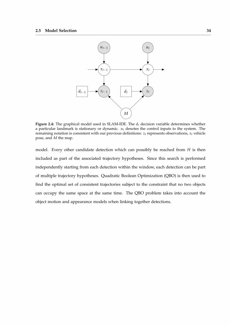
static assumption, as well as the a posteriori probabilities for each of the two cases. Fig. 2.4
shows one time slice of the graphical model used.
More intricate relationships in the data can also be exploited at a systems level without
an explicit probabilistic relationship between the static and dynamic data. This strategy
is used by Leibe et al. [90] for scene modeling from a moving vehicle. Their system com-
bines SfM estimates of the vehicle pose, discriminative detection of pedestrians/vehicles,
and tracking into a single system. To track dynamic objects, they perform a custom op-
timization within a sliding window. For each potential object hypothesis, H, a search is
performed in space-time based on the maximum-velocity of the object under its motion
2.5 Model Selection 34
ut−1 ut
xt−1 xt
zt−1 ztdt−1 dt
M
Figure 2.4: The graphical model used in SLAM-IDE. The dt decision variable determines whethera particular landmark is stationary or dynamic. ut denotes the control inputs to the system. Theremaining notation is consistent with our previous definitions: zt represents observations, xt vehiclepose, and M the map.
model. Every other candidate detection which can possibly be reached from H is then
included as part of the associated trajectory hypotheses. Since this search is performed
independently starting from each detection within the window, each detection can be part
of multiple trajectory hypotheses. Quadratic Boolean Optimization (QBO) is then used to
find the optimal set of consistent trajectories subject to the constraint that no two objects
can occupy the same space at the same time. The QBO problem takes into account the
object motion and appearance models when linking together detections.
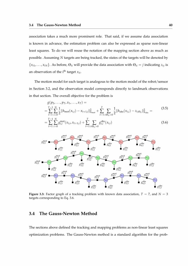
3Background
This chapter provides technical background and introduces the notation which will be used
for the remainder of the thesis. The mathematical notation is introduced in Section 3.1; fol-
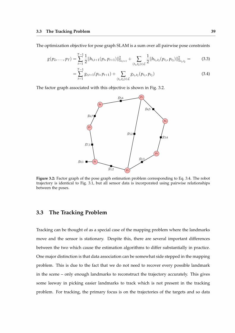
lowing this we provide a brief summary of the typical tracking and mapping problem.
These are specified as objectives to be minimized from the perspective of non-linear opti-
mization rather than the equivalent maximization of log-likelihood.
Section 3.4 describes the Gauss-Newton algorithm as a generic non-linear optimization
procedure applicable to both problems. In order for the Gauss-Newton algorithm to be
applicable to realistic problems, sparse numerical techniques must be used. Various meth-
ods for taking advantage of sparsity are described in Section 3.5 as well the relationship
between sparse estimation and the traditional filtering frameworks used for tracking.
The topic of sparsity naturally leads to a discussion of Gaussian Belief Propagation
(GaBP) as a general framework for taking advantage of sparsity in estimation problems.
Section 3.6 introduces the idea of Gaussian Belief Propagation on Markov Chains, where
the resulting algorithms are equivalent to the Kalman Filter and Kalman Smoother. Fol-
lowing this, Section 3.7 describes the algorithms necessary to generalize GaBP to arbitrary
graphical models.
While there is no novel material presented, we believe there is a gap in the literature of
3.1 Basic Notation 36
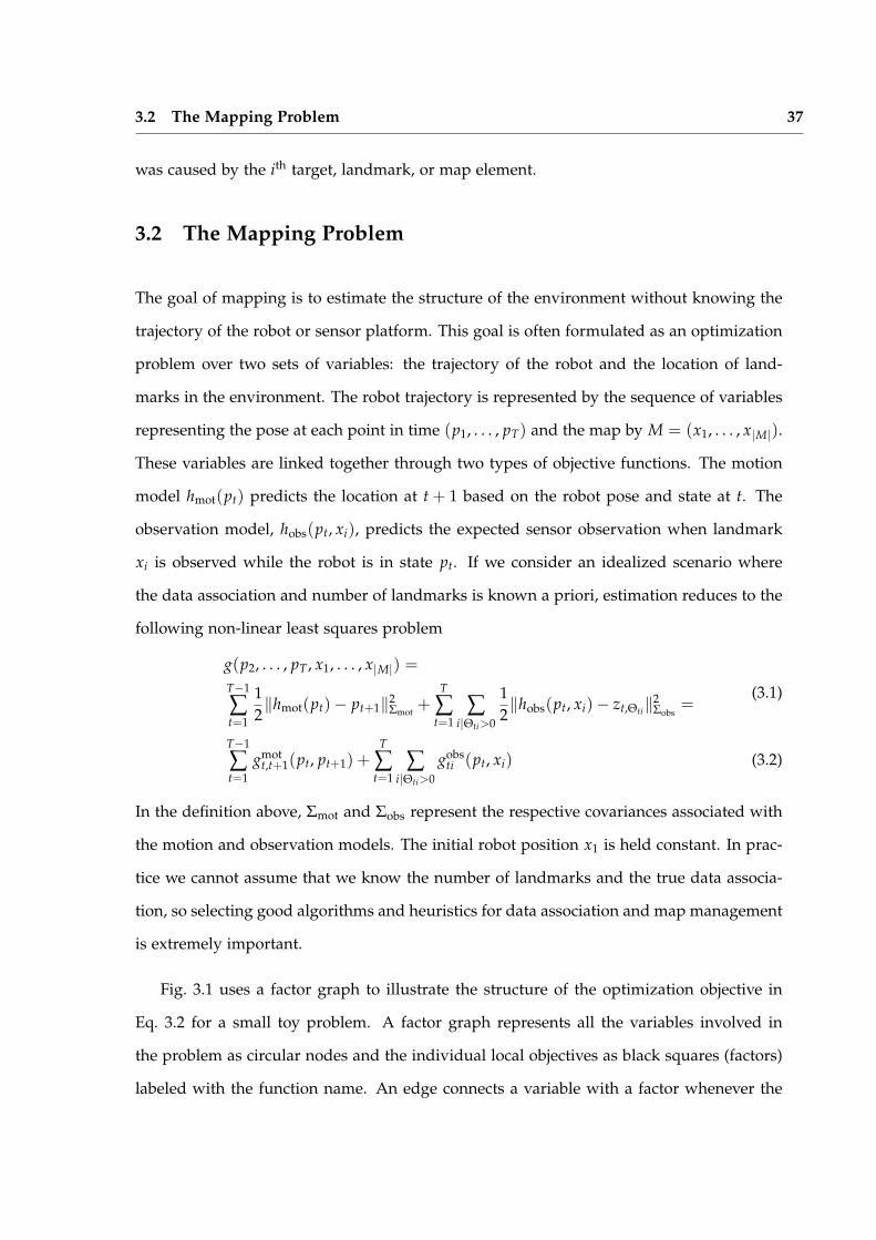
graphical models concerning practical algorithms for generating the commonly referenced
clique trees. As part of an effort to make this thesis self contained, we have provided a more
explicit summary of the relevant algorithms. The majority of this chapter can be skimmed
by a reader already familiar with graphical models, but we would focus attention on the
notation for representing potentials and their associated operations as this will be used
throughout the thesis. In particular, the notation for hybrid discrete/continuous potentials
introduced in Section 3.8 is somewhat unusual, but very useful.
3.1 Basic Notation
This section introduces notation which will be used throughout the thesis. The primary
objects being dealt with can be split up into two categories: observations and the state of
the system being modeled. Observations will generally be denoted as Zt, with t denoting
a time index. When multiple observations are present, Zt will additionally be split as
Zt = (zt1, . . . , zt|Zt|) with |Zt| separate measurements.
The generic system state at time t will be denoted as xt. For the purposes of mapping,
the system state can be split into two components, the time-dependent xt and the global
map denoted by M = (m1, . . . , m|M|) when |M| map elements are present. If multiple
independent states are being tracked, such as in multi-target tracking, the time-dependent
state will be split into multiple components: xt = (xt0, . . . , xtN) for N different dynamic
targets plus one robot. In this case, the robot state will be represented by xt0. When
discrete variables are modeled as part of the system state, they will be denoted as dt for the
discrete modeling variable corresponding to xt.
Data association variables will be denoted by Θ for track-oriented approach (associating
an observation with each landmark/track) and Λ for the measurement-oriented approach
(associating a landmark/track for each observation) Θt will denote the data associations
at time t and Θti = j will correspond to the ith target, landmark or map element being
associated with measurement ztj. Analogously, Λtj = i will indicate that measurement ztj
3.2 The Mapping Problem 37
was caused by the ith target, landmark, or map element.
3.2 The Mapping Problem
The goal of mapping is to estimate the structure of the environment without knowing the
trajectory of the robot or sensor platform. This goal is often formulated as an optimization
problem over two sets of variables: the trajectory of the robot and the location of land-
marks in the environment. The robot trajectory is represented by the sequence of variables
representing the pose at each point in time (p1, . . . , pT) and the map by M = (x1, . . . , x|M|).
These variables are linked together through two types of objective functions. The motion
model hmot(pt) predicts the location at t + 1 based on the robot pose and state at t. The
observation model, hobs(pt, xi), predicts the expected sensor observation when landmark
xi is observed while the robot is in state pt. If we consider an idealized scenario where
the data association and number of landmarks is known a priori, estimation reduces to the
following non-linear least squares problem
g(p2, . . . , pT, x1, . . . , x|M|) =T−1
∑t=1
12‖hmot(pt)− pt+1‖2
Σmot+
T
∑t=1
∑i|Θti>0
12‖hobs(pt, xi)− zt,Θti‖
2Σobs
=(3.1)
T−1
∑t=1
gmott,t+1(pt, pt+1) +
T
∑t=1
∑i|Θti>0
gobsti (pt, xi) (3.2)
In the definition above, Σmot and Σobs represent the respective covariances associated with
the motion and observation models. The initial robot position x1 is held constant. In prac-
tice we cannot assume that we know the number of landmarks and the true data associa-
tion, so selecting good algorithms and heuristics for data association and map management
is extremely important.
Fig. 3.1 uses a factor graph to illustrate the structure of the optimization objective in
Eq. 3.2 for a small toy problem. A factor graph represents all the variables involved in
the problem as circular nodes and the individual local objectives as black squares (factors)
labeled with the function name. An edge connects a variable with a factor whenever the
3.2 The Mapping Problem 38
variable appears in the factor’s domain.
p1
p2
p3
p4
p5
p6
p7
x1
x2
x3
x4
x5
x6
gmot0,1
gmot1,2
gmot2,3
gmot3,4
gmot4,5
gmot5,6
gmot6,7
gobs1,6
gobs1,1
gobs2,1
gobs2,2
gobs3,4
gobs3,3
gobs4,3
gobs4,4
gobs5,4gobs
5,5
gobs5,2
gobs6,5
gobs6,6
gobs7,1
gobs7,6
Figure 3.1: Factor graph of a sample SLAM estimation problem with T = 7 poses and M = 6landmarks corresponding to Eq. 3.2. Red nodes represent robot poses and green nodes representthe landmarks.
Pose graph estimation is an alternative formulation of the mapping problem which
avoids dealing with individual landmarks and instead solves an optimization problem over
only the robot pose variables p1:T. In this case the motion model and observation model are
combined into a single objective hs,t(ps, pt) which encodes an offset between the two poses
and penalizes deviation from this offset according to a metric defined by the covariance Σs,t.
For constraints between two consecutive poses the objective ht−1,t encodes a transformation
estimated from a combination of odometry and sensor data. Constraints between non-
consecutive poses are generated whenever the robot revisits a location and are referred to
as loop closures. The set of loop closures will be referred to as L = (s, t) | ∃hs,t(ps, pt).
3.3 The Tracking Problem 39
The optimization objective for pose graph SLAM is a sum over all pairwise pose constraints
g(p2, . . . , pT) =T−1
∑t=1
12‖ht,t+1(pt, pt+1)‖2
Σt,t+1+ ∑
(t1,t2)∈L
12‖ht1,t2(pt1 , pt2)‖2
Σt1,t2= (3.3)
=T−1
∑t=1
gt,t+1(pt, pt+1) + ∑(t1,t2)∈L
gt1,t2(pt1 , pt2) (3.4)
The factor graph associated with this objective is shown in Fig. 3.2.
p1
p2
p3
p4
p5
p6
p7
g0,1
g1,2
g2,3
g3,4
g4,5
g5,6
g5,2
g6,7
g7,1
Figure 3.2: Factor graph of the pose graph estimation problem corresponding to Eq. 3.4. The robottrajectory is identical to Fig. 3.1, but all sensor data is incorporated using pairwise relationshipsbetween the poses.
3.3 The Tracking Problem
Tracking can be thought of as a special case of the mapping problem where the landmarks
move and the sensor is stationary. Despite this, there are several important differences
between the two which cause the estimation algorithms to differ substantially in practice.
One major distinction is that data association can be somewhat side stepped in the mapping
problem. This is due to the fact that we do not need to recover every possible landmark
in the scene – only enough landmarks to reconstruct the trajectory accurately. This gives
some leeway in picking easier landmarks to track which is not present in the tracking
problem. For tracking, the primary focus is on the trajectories of the targets and so data
3.4 The Gauss-Newton Method 40
association takes a much more prominent role. That said, if we assume data association
is known in advance, the estimation problem can also be expressed as sparse non-linear
least squares. To do we will reuse the notation of the mapping section above as much as
possible. Assuming N targets are being tracked, the states of the targets will be denoted by
xt1, . . . , xtN. As before, Θti will provide the data association with Θti = j indicating ztj is
an observation of the ith target xti.
The motion model for each target is analogous to the motion model of the robot/sensor
in Section 3.2, and the observation model corresponds directly to landmark observations
in that section. The overall objective for the problem is
g(p2, . . . , pT, x1, . . . , xT) =
=T−1
∑t=1
N
∑i=0
12‖hmot(xt,i)− xt+1,i‖2
Σmot+
T
∑t=1
∑i:Θti>0
12‖hobs(xt,i)− zt,Θti‖
2Σobs
=(3.5)
=T−1
∑t=1
N
∑i=0
gmott,i (xt,i, xt+1,i) +
T
∑t=1
∑i:Θti>0
gobst,i (xt,i) (3.6)
x1,1
x2,1
x3,1
x4,1
x5,1
x6,1
x7,1gmot0,1
gmot1,1 gmot
2,1 gmot3,1 gmot
4,1 gmot5,1 gmot
6,1
gobs1,1
gobs2,1
gobs3,1
gobs4,1
gobs5,1
gobs6,1
gobs7,1
x1,2
x2,2
x3,2
x4,2
x5,2
x6,2 x7,2
gmot0,2
gmot1,2
gmot2,2
gmot3,2
gmot4,2 gmot
5,2gmot
6,2
gobs1,2
gobs2,2 gobs
3,2 gobs4,2
gobs5,2
gobs6,2 gobs
7,2
x1,3 x2,3
x3,3 x4,3
x5,3 x6,3
x7,3
gmot0,3
gmot1,3 gmot
2,3 gmot3,3
gmot4,3
gmot5,3 gmot
6,3
gobs1,3 gobs
2,3
gobs3,3 gobs
4,3
gobs5,3 gobs
6,3
gobs7,3
Figure 3.3: Factor graph of a tracking problem with known data association, T = 7, and N = 3targets corresponding to Eq. 3.6.
3.4 The Gauss-Newton Method
The sections above defined the tracking and mapping problems as non-linear least squares
optimization problems. The Gauss-Newton method is a standard algorithm for the prob-
3.4 The Gauss-Newton Method 41
lems defined by Eq. 3.1, Eq. 3.3, and Eq. 3.5. Given a set of objectives gi(xi) : Rni → R,
with xi a (possibly overlapping) subsets of the problem domain x ∈ Rn, the goal is to find
a value for the state vector x which minimizes the combined objective
g = ∑i
gi(xi) (3.7)
We will use the index i to index the objective gi as well as the domain of gi within the global
state vector x. In this notation, xi refers to the elements of x over which gi is defined. For
some situations it will be convenient to use a double index for the set of objectives, i.e. gij.
In this case the corresponding domain will be referred to as xij. To simplify notation, we
define the addition of such sub-vectors so that xi + xj is the sum over corresponding indices.
The missing entries in each of the two vectors are treated as zeros; e.g. we are treating each
xi as a sparse vector in the full problem domain Rn. The same convention will be used
with the gradient vectors and Hessian matrices corresponding to each sub-domain.
The individual gi terms in Eq. 3.7 can be expanded to make the least-squares formula-
tion explicit
gi(xi) =12
fi(xi)> fi(xi) (3.8)
with fi : Rni → Rmi . If we linearize fi at x∗
f [x∗i ]
i (xi) = fi(x∗) +∇ fi(x∗i )>(xi − x∗i ) (3.9)
= fi(x∗) +∇ fi(x∗i )>δi (3.10)
we get the classic Gauss-Newton minimization scheme which iteratively minimizes the
approximate linear least-squares objective
g[x∗](x) = ∑
ig[x
∗]i (xi) = ∑
i
12
f [x∗]
i (xi)> f [x
∗]i (xi) (3.11)
Expanding each term in Eq. 3.11 results in the following quadratic form
g[x∗](x) =∑
i
(12
fi(x∗)> fi(x∗) + fi(x∗)>∇ fi(x∗i )>δi +
12
δ>i ∇ fi(x∗i )∇ fi(x∗i )>δi
)=
12
f (x∗) + gr>δ +12
δ>Hδ
(3.12)
3.5 Sparse Optimization and the Schur Compliment 42
By setting the derivative of Eq. 3.12 to 0, we can compute the optimal δ and use it to update
the linearization point
gr = ∑i
gri = ∑i∇ fi(x∗i )
> fi(x∗i ) (3.13)
H = ∑i
Hi = ∑i∇ fi(x∗i )
>∇ fi(x∗i ) (3.14)
δ = −H−1gr (3.15)
x∗new = x∗ + δ (3.16)
The Gauss-Newton algorithm proceeds by repeating the linearization and quadratic mini-
mization procedure until convergence.
3.5 Sparse Optimization and the Schur Compliment
For large systems of small objectives (i.e. ni n ), the quadratic minimization problem
in Eq. 3.11 is often sparse. This sparsity allows Eq. 3.15 to be scaled to problems with
thousands of variables while still maintaining reasonable performance. There are several
common strategies to do this – some fairly general and some problem specific. To talk about
these approaches it is helpful to visualize the sparsity pattern of the Hessian matrix H. The
sparsity patterns of the Hessians associated with the mapping and tracking optimization
problems are illustrated in Fig. 3.4 and Fig. 3.5. These patterns match the connectivity of
the associated factor graphs (Fig. 3.1, Fig. 3.2, and Fig. 3.3). Since each factor denotes a
relationship between the associated variables, it implies a potential non-zero entry in the
Hessian matrix.
For the SLAM and SfM problems illustrated in Fig. 3.1, block matrix inversion is a
common problem-specific sparsity strategy for solving Eq. 3.15. Looking at Fig. 3.4a, we
can partition the Hessian and gradient into blocks corresponding to the pose and landmark
variables, indicated by the p and x subscripts respectively.[Hpp HpxHxp Hxx
][δpδx
]=
[grpgrx
](3.17)
3.5 Sparse Optimization and the Schur Compliment 43
The decomposition in Eq. 3.17 can be used to take advantage of sparsity by applying Gaus-
sian elimination to the blocks (see Schur compliment, Boyd and Vandenberghe [91]). To do
so solve we first symbolically solve for δx in terms of δp using the second block-row.
δx = H−1xx
(grx −Hxpδp
)(3.18)
The resulting expression is substituted into the second block-row to obtain an equivalent
system in terms of only the x2 variables.
S =Hpp −HpxH−1xx Hxp (3.19)
δp =S−1(
grp −HpxH−1xx grx
)(3.20)
In the above equation S is known as the Schur compliment of Hpp. Once δp is known, the
corresponding value of δx can be computed directly from Eq. 3.18 via back substitution.
The method described above does not reduce computational complexity for dense ma-
trices, but it can help when the Hessian is sparse. Two matrix inverses are needed: H−1xx and
S−1. In Fig. 3.4a we can see that Hxx is a diagonal matrix whose inversion is trivial. On the
other hand, S is of the same size as Hpp and computing S−1 is a relatively small problem
because there are typically far fewer poses than landmarks. This technique is often referred
to as the Schur compliment trick and has a long history in the literature [92].
More general sparse matrix decomposition algorithms can take advantage of arbitrary
matrix sparsity when solving the quadratic optimization problem [93]. These techniques
are also applicable to pose graph estimation, where there is no guarantee that any particular
submatrix has diagonal or block diagonal structure.
For the special case of multi-target tracking, a Kalman filter is often used for each of
the trajectories shown in Fig. 3.5. The Kalman filter can also be thought of as a sparse
linear-least squares algorithm [16, 18] and at its core also relies on iterative application of
the Schur compliment trick. The following section will illustrate that Gaussian Graphical
Models can be thought of as a generalization of this idea to arbitrary sparse problems.
3.5 Sparse Optimization and the Schur Compliment 44
H =
p1 p2 p3 p4 p5 p6 p7 x1 x2 x3 x4 x5 x6
p1
p2
p3
p4
p5
p6
p7
x1
x2
x3
x4
x5
x6
(a) SLAM/SfM formulation of the mapping problem
H =
p1 p2 p3 p4 p5 p6 p7
p1
p2
p3
p4
p5
p6
p7
(b) Pose graph formulation of the mapping problem
Figure 3.4: Typical sparsity patterns for mapping problems.
3.5 Sparse Optimization and the Schur Compliment 45
H =
H1 0 00 H2 00 0 H3
H1 =
x11 x21 x31 x41 x51 x61 x71
x11
x21
x31
x41
x51
x61
x71
H2 =
x12 x22 x32 x42 x52 x62 x72
x12
x22
x32
x42
x52
x62
x72
H3 =
x13 x23 x33 x43 x53 x63 x73
x13
x23
x33
x43
x53
x63
x73
Figure 3.5: Typical sparsity pattern for multi-target tracking problems. Note that the estimationproblem for each track is in fact completely independent. While it is not common to think of this asproblem sparsity, it is in fact an extreme example where the estimation for each track is completelyindependent once data association is established.
3.6 Gaussian Belief Propagation: Markov Chains 46
3.6 Gaussian Belief Propagation: Markov Chains
Gaussian Belief Propagation is a probabilistic alternative to the linear algebra based ap-
proaches to sparsity discussed in the previous section. Since maximum likelihood infer-
ence in a linear Gaussian model is equivalent to linear least-squares, we can switch to a
probabilistic perspective in order to take advantage of well developed sparse inference al-
gorithms. Gaussian Belief Propagation is an application of Belief Propagation to Gaussian
graphical models [94, 95]. The resulting algorithm is very similar to the block Gaussian
elimination techniques described in the previous section. This connection to graphical
models and general inference techniques motivates the inclusion of discrete variables in
Chapter 4. A detailed presentation of these topics is beyond the scope of this thesis, but we
will provide an overview geared towards defining the notation and providing a reference
for the remaining chapters.
3.6.1 Belief Propagation and Message Passing
The Belief Propagation algorithm is a very general application of dynamic programming to
sparse inference. It is applicable to both MAP inference and the computation of posterior
distributions. We use a simple estimation problem as an example to introduce the topic
at an intuitive level. The problem consists of estimating the state of a system of three
variables (x1, x2, x3) ∈ R3 from the corresponding observations (z1, z2, z3). The posterior
for this problem is proportional to the following product
P(x1:3 | z1:3) ∝ P(z1 | x1)P(x1)︸ ︷︷ ︸L(x1)
P(z2 | x2)P(x2 | x1)︸ ︷︷ ︸L(x1,x2)
P(z3 | x3)P(x3 | x2)︸ ︷︷ ︸L(x2,x3)
(3.21)
The MAP estimate is given by
x∗1:3 = argmaxx1:3
L(x1)L(x1, x2)L(x2, x3)
(3.22)
Assuming all of the component distributions in Eq. 3.21 are Gaussian, we can compute x∗1:3
by computing the parameters of the distribution P(x1:3 | z1:3) and looking at its mean.
3.6 Gaussian Belief Propagation: Markov Chains 47
Despite the fact that we know x1 and x3 do not directly interact, this information is
lost once we compute P(x1, x2, x3). As an alternative, we can incrementally compute the
maximal values while reusing the partial computations as much as possible; this is the
dynamic programming approach. For the example above, we can rewrite the maximization
to emphasize the repetitive computations inherent in the calculation.
x∗1 = argmaxx1
max
x2
L(x1)L(x1, x2)max
x3
L(x2, x3)
(3.23)
x∗2 = argmaxx2
max
x1
L(x1)L(x1, x2)
max
x3
L(x2, x3)
(3.24)
x∗3 = argmaxx3
max
x2
max
x1
L(x1)L(x1, x2)
L(x2, x3)
(3.25)
The repetition becomes more obvious if we define temporary distributions φ1(x1, x2), φ2(x2, x3),
−→µ (x2), and←−µ (x2) as follows
x∗1 = argmaxx1
max
x2
φ1(x1,x2)︷ ︸︸ ︷L(x1)L(x1, x2)max
x3
φ2(x2,x3)︷ ︸︸ ︷L(x2, x3)
︸ ︷︷ ︸
←−µ (x2)
(3.26)
x∗2 = argmaxx2
max
x1
φ1(x1,x2)︷ ︸︸ ︷L(x1)L(x1, x2)
︸ ︷︷ ︸
−→µ (x2)
maxx3
φ2(x2,x3)︷ ︸︸ ︷L(x2, x3)
︸ ︷︷ ︸
←−µ (x2)
(3.27)
x∗3 = argmaxx3
max
x2
max
x1
φ1(x1,x2)︷ ︸︸ ︷L(x1)L(x1, x2)
︸ ︷︷ ︸
−→µ (x2)
φ2(x2,x3)︷ ︸︸ ︷L(x2, x3)
(3.28)
The temporary distributions φ1 and φ2 are referred to as the local potentials; these capture
the local relationships between variables. The other two temporary distributions, −→µ and
←−µ , are referred to as messages. The forward message −→µ captures all information about
x2 from φ1. Similarly, the backward message ←−µ captures all information about x2 from
φ2. The messages transmit information between the two local potentials and allow a global
solution to be coordinated. Belief propagation, when run on this example results in the
3.6 Gaussian Belief Propagation: Markov Chains 48
follow computations
φ1(x1, x2) ..=L(x1)L(x1, x2) (3.29)
φ2(x2, x3) ..=L(x2, x3) (3.30)
−→µ (x2) ..=maxx1
φ1(x1, x2)
(3.31)
←−µ (x2) ..=maxx3
φ2(x2, x3)
(3.32)
B1(x1, x2) ..=φ1(x1, x2)←−µ (y) (3.33)
B2(x2, x3) ..=φ2(x2, x3)−→µ (y) (3.34)
(x∗1 , x∗2) ..= argmaxx1,x2
B1(x1, x2)
(3.35)
(x∗2 , x∗3) ..= argmaxx2,x3
B1(x1, x2)
(3.36)
After computing the local potentials and the messages, results are stored in the ’belief’
distributions B1 and B2. These combine information from the local potentials with the
incoming message in order to compute a proxy for the global objective over the local vari-
ables. Note that despite the fact that x∗2 is computed twice, the optimal values will be
the same as long as all of the local potentials are not degenerate distributions. This is a
consequence of the fact that non-degenerate Gaussian distributions have a unique maximal
likelihood value.
The intuition behind the Belief Propagation algorithm is similar to block Gaussian elim-
ination algorithm. Instead of maximizing L(x1, x2, x3) over (x1, x2, x3), we are symbolically
maximizing φ1 over x1 in closed form before combining it with φ2 to compute the maxi-
mal value over (x2, x3). In this particular example, there is not much of a computational
advantage due to the overhead of the algorithm compared to the amount of sparsity in the
problem. For larger problems the improvement can be drastic. If each of x1, x2, and x3
represented n-dimensional vectors instead of single variables, the algorithm above would
replace a least-squares problem of size 3n with several problems of size 2n. Due to the
roughly O(n3) computational cost of Cholesky decomposition, this makes a larger differ-
ence as n increases.
3.6 Gaussian Belief Propagation: Markov Chains 49
3.6.2 Gaussian Potentials
Gaussian Belief Propagation requires manipulating various Gaussian distributions in closed
form. To do so we must define data structures capable of storing the various potentials as
well as the set of allowed operations on these data structures (e.g. maximization, inte-
gration, and computing products). For many of the required operations, the ’information
form’ of the Gaussian distribution is a much more convenient parameterization than the
standard moment form. In addition, the information matrix naturally corresponds to the
Hessian matrix and so directly reveals the sparsity structure of the problem. This is not
the case with the covariance matrix, which is typically dense even for sparse Gaussian
distributions.
The probability density function of x ∼ N (µ, Σ) is given by
P(x | µ, Σ) = (2π)−n2 |Σ|−
12 exp
(−1
2(x− µ)>Σ−1(x− µ)
)(3.37)
Instead of the moments µ and Σ, the information form is defined via the information matrix
I and the information vector η
I ≡ Σ−1 (3.38)
η ≡ Σ−1µ (3.39)
We can rewrite the density from Eq. 3.37 in information form by expanding the term inside
the exponent and applying the above definitions
P(x | η, I) = (2π)−n2 |I|
12 exp
(−1
2x> Ix + x>η − 1
2η> I−1η
)(3.40)
We note that the log-likelihood of Eq. 3.40 is always a quadratic form in x
log P(x) =− n2
log(2π) +12
log|I|+(−1
2x> Ix + x>η − 1
2η> I−1η
)(3.41)
=12
x>(−I)x + x>η +
(12
log|I| − n2
log(2π)− 12
η> I−1η
)(3.42)
=12
x>Ax + x>b + c (3.43)
3.6 Gaussian Belief Propagation: Markov Chains 50
This motivates the definition of a general Gaussian Potential, φ(x) as the exponent of a
quadratic form. The Gaussian Potential φ : Rn → R is represented by the three parameters
Aφ, bφ, and cφ such that
φ(x) ≡ exp(
12
x>Aφx + x>bφ + cφ
)(3.44)
This definition does not always correspond to a valid Gaussian distribution, but any Gaus-
sian distribution can be represented as above. To represent a standard multivariate Gaus-
sian with information parameters (I, η), the potential parameters are set to
Aφ = −I (3.45)
bφ = η (3.46)
cφ =12
log|I| − n2
log(2π)− 12
η> I−1η (3.47)
Gaussian Potentials can also be used to represent conditional distributions where the
mean is parameterized by an affine function
x | y ∼ N (µ(y), Σ) (3.48)
µ(y) = Hy + µ0 (3.49)
If we write the information vector, η, as a function of y and express the log-likelihood in
terms of the parameters I, y, and µ0 we get
η(y) = I(Hy + µ0) (3.50)
log P(x | y) = −n2
log(2π) +12
log|I| − 12
x> Ix + x>η(y)− 12
η(y)> I−1η(y) (3.51)
By expanding the definition of η(y) and rearranging terms, we can rewrite Eq. 3.51 as a
quadratic form of the combined vector (x, y) parametrized by I, H, and µ0
log φ(x, y) ≡ log P(x | y) = 12
[xy
]>[Axx AxyAyx Ayy
][xy
]+
[xy
]>[bxby
]+ c (3.52)
3.6 Gaussian Belief Propagation: Markov Chains 51
with
Axx = −I (3.53)
Axy = A>yx = IH (3.54)
Ayy = −H> IH (3.55)
bx = Iµ0 (3.56)
by = −H> Iµ0 (3.57)
c =12
(µ>0 Iµ0 + n log(2π)− log|I|
)(3.58)
The potentials are closed under multiplication, division, and exponentiation. That is,
φ1 ∗ φ2, φ1/φ2, and φα1 are all valid potentials. As an example, the multiplication of two
potentials φ1 ∗ φ2 results in the product potential φprod with parameters
Aφprod = Aφ1 + Aφ2 (3.59)
bφprod = bφ1 + bφ2 (3.60)
cφprod = cφ1 + cφ2 (3.61)
These properties are a consequence of the definition in Eq. 3.44 and the linearity of quadratic
forms in terms of their parameters. When multiplying or diving two potentials which do
not have the same domain, e.g. φprod(x, y, z) = φ1(x, y) · φ2(y, z) the factor potentials are
extended to cover the full domain (x, y, z). This is done by setting the quadratic form pa-
rameters correspond to the added variables to zero. Letting A1, b1, c1 and A2, b2, c2 be the
parameters of φ1 and φ2 respectively, the product parameters are computed as
Aφprod =
A1xx A1xy 0A1yx A1yy 0
0 0 0
+
0 0 00 A2yy A2yz0 A2zy A2zz
(3.62)
bφprod =
b1xb1y0
+
0b2yb2z
(3.63)
cφprod =c1 + c2 (3.64)
The operations φa · φb and φa/φb are defined in terms of the respective sum and different
of the parameters of the quadratic forms.
3.6 Gaussian Belief Propagation: Markov Chains 52
If a potential φ is negative semi-definite, that is the matrix Aφ is negative semi-definite,
we can also compute integrals and maximize in closed form. To do so for the potential
φ(x, y) we partition its parameters into blocks corresponding to the x ∈ Rn and y ∈ Rm
variables
Aφ =
[Axx AxyAyx Ayy
]∈ R(n+m)×(n+m) (3.65)
bφ =
[bxby
]∈ Rn+m (3.66)
Using the partitioned parameters, φmarg(x) =∫
φ(x, y)dy is given by
Aφmarg = Axx − Axy A−1yy Ayx (3.67)
bφmarg = bx − Axy A−1yy by (3.68)
cφmarg = cφ −12
b>y A−1yy by +
12
m log(2π)− 12
log∣∣−Ayy
∣∣ (3.69)
Similarly, φmax(x) = maxy
φ(x, y)
has parameters
Aφmax = Axx − Axy A−1yy Ayx (3.70)
bφmax = bx − Axy A−1yy by (3.71)
cφmax = cφ −12
b>y A−1yy by; (3.72)
Note that the only difference between maximization and marginalization of Gaussian Po-
tentials is the constant factor in the quadratic form. Maximization and marginalization
(integration) of potentials will be a commonly used operation in this thesis, so we define
the following operators as short hand for the operations described above.
margy
[φ] ≡∫
φ(x, y)dy (3.73)
maxy
[φ] ≡maxy
φ(x, y)
(3.74)
These operators take a potential as input and return a modified potential representing the
result of the specified operation.
Finally, it is occasionally useful to define a conditioning or partial evaluation operation
for Gaussian Potentials. This comes into play when a probabilistic model needs to be
3.6 Gaussian Belief Propagation: Markov Chains 53
conditioned on actual observations prior to inference. Given φ(x, y) parameterized as in
Eq. 3.65 and Eq. 3.66, we can define a partial evaluation operation which fixes y = y0 at a
single value. The potential φeval(x) = φ(x, y=y0) has parameters given by
Aφeval = Axx (3.75)
bφeval = bx + Axyy0 (3.76)
cφeval = cφ + b>y y0 +12
y>0 Ayyy0; (3.77)
This operation is efficient in information form as it does not require any matrix inversions.
In the covariance parameterization, computing the parameters of a partial evaluation oper-
ation requires computing the Schur complement.
3.6.3 The Kalman Filter and Smoother
Using the principles from Section 3.6.1 and the operations from Section 3.6.2 we can define
the Kalman Filter and Smoother as special cases of Belief Propagation. If the motion and
observation models are linear with Gaussian noise, we can define local potentials for each
t
φ1(x1) ≡P(x1)P(z1 | x1) (3.78)
φ2(x1, x2) ≡P(x2 | x1)P(z2 | x2) (3.79)...
φt(xt−1, xt) ≡P(xt | xt−1)P(zt | xt) (3.80)...
Given the graphical model and clique tree shown in Fig. 3.6 combined with the po-
tentials defined above, the message passing algorithm is composed of the following basic
3.6 Gaussian Belief Propagation: Markov Chains 54
x1 x2 · · · xT
z1 z2 · · · zT
(a) Bayesian Network
φ1(x1) φ2(x1, x2) · · · φT(xT−1, xT)
−→µ 1(x1)
←−µ 2(x1)
−→µ 2(x2)
←−µ 3(x2)
−→µ T−1(xT−1)
←−µ T(xT−1)
(b) Clique tree
Figure 3.6: Graphical model and associated clique tree for the filtering/smoothing problem.
]20: for t = T − 1, . . . , 2 do21: ←−µ t(xt−1) ..= maxxt
[φt(xt−1, xt) · ←−µ t+1(xt)
]. Eq. 3.82
22: end for23: return
←−µ t
. Return the computed set of backward messages24: end procedure
Figure 3.7: The Forward-Backward algorithm for Linear Dynamical Systems
3.7 Gaussian Belief Propagation: General Graphs
The previous section introduced the intuition for Gaussian Belief Propagation and the prac-
tical algorithm for Markov Chains. In this section we will describe how to apply the same
techniques to more general problem structures. The generalized procedure requires a sub-
stantial amount of preprocessing in order to generate the appropriate graph structures.
First, we must convert the factor graph representation of the problem to a Markov Random
Field. The Markov Random Field is then used to compute a variable elimination ordering
which in turn generates an elimination tree. At the final stage of the preprocessing, the
elimination tree is modified to produce a clique tree. This final clique tree data structure
3.7 Gaussian Belief Propagation: General Graphs 56
can be used by the Belief Propagation algorithm to partition the sparse global problem
into a tree-structured network of small dense local sub-problems. The four stages of this
preprocessing are shown in Fig. 3.8. The algorithms presented here are based on Dawid
et al. [95] which should be consulted for further details.
To describe the general case, it is easiest to use Markov Random Fields (MRFs) as a
representation of sparsity. A MRF graph contains a vertex for every variable in the problem
and an edge between two variables whenever there is a direct relationship between them.
Specifically, an edge between two variables indicates that they are present together in the
domain of at least one objective/local potential. To convert from a factor graph to an
MRF representation, we simply remove all of the factors in the factor graph. For each
factor removed, edges are added so that the variables in its domain form a clique. As an
example, Fig. 3.8a demonstrate the MRF corresponding to the factor graph in Fig. 3.2.
3.7 Gaussian Belief Propagation: General Graphs 57
p1
p2
p3
p4
p5
p6
p7
(a) Markov Random Field corresponding tothe factor graph in Fig. 3.2.
p1
p2
p3
p4
p5
p6
p7
(b) Triangulation induced by the elimina-tion ordering p1, p3, p4, p2, p5, p6, p7. Dashededges have been added by the triangulation.
p1 : p1, p2, p7 p3 : p3, p2, p4
p4 : p4, p2, p5
p2 : p2, p5, p7
p5 : p5, p6, p7
p6 : p6, p7
p7 : p7
(c) Elimination tree corresponding to theelimination ordering.
p1 : p1, p2, p7
p2 : p2, p5, p7
p4 : p4, p2, p5
p3 : p3, p2, p4
p5 : p5, p6, p7
(d) Clique tree generated from the elimina-tion tree by keeping only the vertices corre-sponding to maximal cliques.
Figure 3.8: Illustration of the graphs involved in converting the factor graph in Section 3.2 to aclique tree which can be used for inference or optimization.
3.7 Gaussian Belief Propagation: General Graphs 58
3.7.1 Variable Elimination Orderings
The concept of an elimination ordering is central to generalizing Section 3.6. To do so we
consider the problem of efficiently finding the maximal likelihood value itself (or marginal
likelihood when computing a posterior). This is done by eliminating variables from the
problem one at a time via partial maximization (or marginalization). Each elimination
solves the optimization problem in terms of a single variable and produces a smaller, equiv-
alent problem. However, each elimination has the potential to offset the decrease in prob-
lem size by also decrease sparsity. To avoid this, it is important to choose an elimination
order carefully. Once the ordering is established, it can be used to compute the actual value
of all variables by using a generalization of the dynamic programming/message passing
techniques in Section 3.6.
The process for eliminating a variable starts by collecting all factors which are adjacent
to it in the factor graph. This set of factors is replaced by a single combined factor where
the target variable has been eliminated in closed form. The domain of the newly created
factor is the set of neighbors of the target variable in the MRF. The actual elimination than
reduces the size of this domain by one. In the three variable example from Section 3.6.1,
the optimal elimination order is x1, x2, x3 (or the reverse). This ordering corresponds to the
following expression for computing the maximum likelihood value
v∗ = maxx3
max
x2
P(x3 | x2)max
x1P(x1)P(x2 | x1)︸ ︷︷ ︸
ψ1(x1,x2)
︸ ︷︷ ︸ψ2(x2,x3)
︸ ︷︷ ︸ψ3(x3)
(3.84)
Eliminating the variables in the wrong order, for example the ordering x2, x3, x1, corre-
sponds to the expression
v∗ = maxx1
max
x3
max
x2P(x1)P(x2 | x1)P(x3 | x2)︸ ︷︷ ︸
ψ1(x1,x2,x3)︸ ︷︷ ︸ψ2(x1,x3)
︸ ︷︷ ︸ψ3(x1)
(3.85)
3.7 Gaussian Belief Propagation: General Graphs 59
By eliminating x2 in the inner-most part of the evaluation, we are forced to incorporate
all factors involving x2 into a single potential and do not gain anything from the problem
sparsity. Eliminating blocks of variables in the appropriate order, however, can reduce
the total computational effort. Unfortunately finding the optimal elimination order in an
arbitrary graph is an NP-complete problem, the solution of which requires heuristics in
practice [96].
Heuristic algorithms for variable elimination are based on considering the sequence of
temporary potentials (ψ1, ψ2, ψ3) created in the elimination process, as labeled above in
Eq. 3.84 and Eq. 3.85. In the case of the the sub-optimal ordering shown in Eq. 3.85, the
ψ1 temporary potential is defined over all three variables, and so this ordering negates any
possible savings due to sparsity. In contrast, Eq. 3.84 never constructs a potential with
domain size greater than two. To visualize the resulting loss of sparsity, we can modify the
original MRF by adding the edges necessary to represent the full sequence of temporary
potentials. The resulting graph is the ’triangulation’ of the original MRF. The edges added
in this way are referred to as fill-in; our goal will be to minimize the amount of such added
edges. Note that in the Markov Chain example from the previous section, the natural
sequential ordering of the variables is optimal and does not cause any fill-in.
The typical heuristic for computing the elimination ordering, shown in Fig. 3.9, al-
ways attempts to eliminate the variable which will minimize fill-in. To pick which of the
remaining variables to eliminate at step i, the algorithm attempts to minimize the size
of the domain of the temporary potential φi. As a side effect, we also generate a set
of temporary potential domains C[xi]i which correspond to cliques in the triangulated
graph. Applying this heuristic to the MRF in Fig. 3.8a results in the triangulated graph
shown in Fig. 3.8b where the dashed edges represent fill-in. The corresponding ordering
is: (p1, p3, p4, p2, p5, p6, p7).
3.7 Gaussian Belief Propagation: General Graphs 60
1: procedure EliminationOrder(G ≡ (V , E), H)2: for i ∈
1, . . . , |V|
do
3: u ..= argminv∈G.V H(G, v) . Pick next variable using heuristic H4: N ..= neighbors(G, u)5: G ..= G\u . Remove u along with all adjacent edges6: E ..= E ∪
(i, j)|i, j ∈ N
. Add induced edges between neighbors
7: O[u] ..= i . Store vertex ordering8: C[u] ..= N ∪ u . Store the elimination clique9: end for
10: return (O, C) . Return the ordering and associated cliques11: end procedure
12: procedure H(G, v)13: return |neighbors(G, v)| . The minimum degree heuristic14: end procedure
Figure 3.9: Computing a variable elimination ordering for a Markov Random Field.
3.7.2 Elimination Trees
The variable elimination ordering computed using Fig. 3.9 is in fact not a total ordering,
but a partial order relation. There are sequences of variables which must be eliminated in a
fixed order, but different portions of the graph are often independent of each other and can
in fact be eliminated in parallel. This gives rise to the concept of an elimination tree. Each
node in the elimination tree corresponds to a variable. The root of the tree corresponds to
the last variable to be eliminated. The partial ordering is encoded by the rule that a parent
can only be eliminated after all of its children, whereas siblings can be eliminated in any
order. An example of an elimination tree is shown in Fig. 3.8c. Each node is labeled as
v : c1, c2, . . . where v is the variable being eliminated and c1, c2, . . . is the domain of
the required temporary potential.
An elimination tree can be build with Fig. 3.10 using the previously computed elimina-
tion ordering O and cliques C. For each vertex v in the ordering O, v must be eliminated
before the set of neighbors C[v] to ensure that the domains of the temporary potential
is not altered. This can be guaranteed by making sure that v is eliminated before any
u ∈ neighbors(v).
3.7 Gaussian Belief Propagation: General Graphs 61
1: procedure EliminationTree(V , O, C)2: E ..= ∅ . T ≡ (V , E)3: for v ∈ V do4: N ..= C[v]\v . Clique of non-eliminated neighbors when v is eliminated5: p ..= argminu∈N
O[u]
. Parent is next (in O) neighbor to be eliminated
6: E ..= E ∪ (p, v) . Create a p→ v edge in T7: end for8: return T ≡ (V , E) . Return the elimination tree9: end procedure
Figure 3.10: Constructing an elimination tree from the vertices V , ordering O, and the associatedcliques C.
3.7.3 Clique Trees
A clique tree is the final data structure needed in order to perform inference. It is almost
identical to the elimination tree, but can be more compact by grouping long chains of
eliminations into a single operation. The variable sets in the elimination tree correspond
to domains of the temporary potentials, each of which forms a clique in the triangulated
graph. Each node in the clique tree corresponds to a maximal clique in the triangulated
graph. A clique tree is a network of these maximal cliques which encode a whole set of
elimination orderings as shown in Fig. 3.8d. To extract a particular elimination ordering,
we must choose which set of variables we would like to be eliminated last and define this
clique as the root of the tree. The resulting elimination ordering is always consistent with
the triangulated graph. The elimination process starts at the leaves of the clique tree and
proceeds towards the root. Traversing an edge from node u to v requires eliminating all
variables in the set C[u]\C[v]. In Fig. 3.8d traversing the path p3 → p4 → p2 → p5 is
equivalent to eliminating the variables p3, p4, followed by p2. The path p5 → p2 →
p1 corresponds to eliminating p6, p7, followed by p5.
An elimination tree from the previous section can be converted into a clique tree using
the algorithm shown in Fig. 3.11. This algorithm is based on two properties of the elimi-
nation tree. First, each maximal clique of the triangulated graph has a corresponding node
in the elimination tree (the converse is not true). Second, the elimination cliques in the
tree are nested. That is, variables are always eliminated as we move up the tree. This im-
3.7 Gaussian Belief Propagation: General Graphs 62
plies the maximal cliques can be identified by comparing the elimination set of each node
with that of its children. Removing the non-maximal cliques in the elimination tree results
in a clique tree which can be used for inference. The removal of non-maximal cliques is
performed using a contraction operation on edges in the tree. Whenever a clique is found
which is a subset of one of its children, the two vertices are merged by contracting their
shared edge. After running this algorithm, all remaining elimination sets are guaranteed
to be maximal and so the elimination tree becomes a clique tree. The clique tree for the
pose graph example is shown in Fig. 3.8d.
1: procedure CliqueTree(T ≡ (V , E), O, C)2: for v ∈ V do . Go through all nodes in the elimination tree3: for u ∈ children(v) do4: if C[v] ⊂ C[u] then . If v has a child whose clique is a super set5: u∗ ..= contract(u, v) . Merge u and v into a single vertex6: C[u∗] ..= C[u] . Set the clique of u∗ to the larger clique7: T ..=
(T \u, v
)∪ u∗ . Replace u and v with u∗
8: break9: end if
10: end for11: end for12: return T ≡ (V , E) . Return the clique tree13: end procedure
Figure 3.11: Converting an elimination tree into a clique tree.
3.7.4 Belief Propagation on Clique Trees
As already mentioned, a clique tree encodes a set of variable elimination orderings to effi-
ciently solve for the values of any maximal clique in the triangulated graph. The Forward-
Backward algorithm described in Section 3.6 used dynamic programming and temporary
message potentials to simultaneously compute the posterior over all variable in the chain.
The full Belief Propagation algorithm is a generalization of this idea to the clique tree. It
simultaneously computes all possible sequences of variable eliminations encoded by the
tree and so solves the problem for all variables. For example, the expression for the local
3.7 Gaussian Belief Propagation: General Graphs 63
posterior at over the C2 domain is given by the following formula
B2(p2, p5, p7) =φ2 · µ5,2 · µ1,2 · µ4,2 = (3.86)
=φ2 ·(max
p6[φ5]︸ ︷︷ ︸
µ5,2
)·(max
p1[φ1]︸ ︷︷ ︸
µ1,2
)·(max
p4[φ4 · µ3,4]︸ ︷︷ ︸µ4,2
)(3.87)
=φ2 ·(max
p6[φ5]︸ ︷︷ ︸
µ5,2
)·(max
p1[φ1]︸ ︷︷ ︸
µ1,2
)·(max
p4[φ4 ·max
p3[φ3]︸ ︷︷ ︸
µ3,4
]
︸ ︷︷ ︸µ4,2
)(3.88)
The general dynamic programming recursion for the posterior with a clique tree T =
(V , E) is
Bi =φi · ∏j∈neighbors(i)
µj,i ∀i ∈ V (3.89)
µi,j = maxC[i]\C[j]
[φi · ∏
k∈neighbors(i)\jµk,i
]∀(i, j) ∈ E (3.90)
The message potentials µi,j are labeled with two indices specifying, respectively, the source
and target vertex in the clique tree. This recursion makes it possible to simultaneously
compute the posterior over all domains. In practice, the recursive equations are imple-
mented in two rounds of message passing as shown in Fig. 3.13. The initial upward pass
computes all the messages from the leaves to the root of the clique tree. The downward
pass computes the messages from the root back towards the leaves. Fig. 3.12 illustrates the
algorithm on the clique tree example from the previous section.
3.7 Gaussian Belief Propagation: General Graphs 64
Figure 3.12: Clique tree with annotated messages; the message passing root outlined in bold.Fig. 3.13 lists the general algorithm for computing the messages and posterior beliefs.
3.7 Gaussian Belief Propagation: General Graphs 65
1: procedure BeliefPropagation(T ≡ (V , E), φvv∈V )2: R ..= root(T )3: UpwardPass(R) . Gather information from the leaves upward4: DownwardPass(R) . Distribute information from the root downward5: for v ∈ V do . Compute the posterior beliefs6: Bv(xv) ..= φv(xv) ·∏u∈neighbors(v) µu,v(xu∩v)7: end for8: return Bvv∈V . Return the set of posterior beliefs9: end procedure
10: procedure UpwardPass(v)11: for c ∈ children(v) do12: UpwardPass(c)13: end for14: p ..= Parent(v)
15: µv,p(xv∩p) ..= maxxv\p
[φv(xv) · ∏
c∈children(v)µc,v(xc∩v)
]16: end procedure
17: procedure DownwardPass(v)18: for c ∈ children(v) do
19: µv,c(xv∩c) ..= maxxv\c
[φv(xv) · ∏
d∈neighbors(v)\cµd,v(xd∩v)
]20: DownwardPass(c)21: end for22: end procedure
Figure 3.13: The Belief Propagation algorithm over a clique tree. The domain of each vertex/cliqueis denoted by xv ≡ C[v]. The message domains correspond to intersections of the clique domainsand are written as xu∩v ≡ C[u]∩C[v]. Similarly, xv\u ≡ C[v]\C[u] denotes the set difference domain.
3.8 Discrete Variables and Hybrid Potentials 66
3.8 Discrete Variables and Hybrid Potentials
This dissertation is focused on incorporating discrete variables into the purely continuous
problems which can be described with Gaussian Graphical Models and solved with mes-
sage passing. Up to this point we have reviewed inference and optimization in continuous
systems, but have avoided the topic of discrete variables and model selection. This sec-
tion focuses on adding discrete variables to the Gaussian Potentials from Section 3.6.2 and
demonstrates why this addition breaks the inference algorithms discussed above.
As a first step, we will define the notation for local potentials which depend on discrete
variables. A hybrid potential φ(x, d) is a function of both continuous variables x ∈ Rn
and discrete variables d ∈
1, . . . , K
. Such a hybrid potential is essentially a table of K
different Gaussian Potentials, each conditioned on a possible value of d
φ(x, d=k) ≡φ(k)(x) ∀k ∈
1, . . . , K
(3.91)
φ(k)(x) ≡12
x>A(k)x + x>b(k) + c(k) ∀k ∈
1, . . . , K
(3.92)
The parameterization of the discrete potential φ(x, d) is formally defined as a table of
quadratic forms, each one equivalent to one of the Gaussian Potentials in
φ(k)A(k)
φ =Aφ(k) ∀k ∈
1, . . . , K
(3.93)
b(k)φ =bφ(k) ∀k ∈
1, . . . , K
(3.94)
c(k)φ =cφ(k) ∀k ∈
1, . . . , K
(3.95)
The difficulty with hybrid potentials is that they are not closed under the partial marginal-
ization and maximization operations required for efficient inference. In the case of the
φ(x, d) as defined above, we can define margd(φ) as
margd
[φ(x, d)
]≡
K
∑i=1
φ(x, d = i) (3.96)
Unfortunately, there is no way to compactly represent the right hand side of Eq. 3.96 with-
out explicitly storing the parameters of each φ(k) in a table and adding up the K different
3.8 Discrete Variables and Hybrid Potentials 67
values whenever we need to evaluate margd[φ](x) for a particular value of x (the situation
with maxd[φ]
is identical). Without a closed form representation, taking the product of
successive hybrid potentials results in a table with an exponentially increasing number of
entries. Unlike the Gaussian case where the brute force approach is at worst cubic, hybrid
Belief Propagation is fundamentally intractable without approximations. In the following
chapter we will introduce our approximation strategy to avoid this problem.
4Iterative Local Model Selection
4.1 Introduction
The major limiting factor in applying switching models to perception is a lack of general
purpose inference algorithms. In order to be useful for the large scale estimation problems
described in the introduction, such an algorithm must satisfy a few basic requirements:
• It must take advantage of sparsity and be able to scale to problems with tens of
thousands of variables
• It should not require domain specific tuning parameters or heuristics
• It should work reliably, avoiding unpredictable failure modes
This chapter introduces the Iterative Local Model Selection (ILMS) algorithm as a novel
approximate inference technique for SLDS models, and validates the algorithm against
these basic requirements above.
The initial development of the algorithm is described in the context of Switching Lin-
ear Dynamical Systems (SLDS) rather than the more general Conditional Linear Gausian
Networks. Chapter 6 will introduce the necessary modifications for the more general case.
SLDS time series models are a powerful generalization of Linear Dynamical Systems which
4.2 Switching Linear Dynamical Systems 69
include a set of discrete variables controlling the behavior of the otherwise linear system.
The discrete variables form a Markov process whose value acts as a switch controlling
which linear model is in play. In other words, the parameters of the observation and tran-
sition model are governed by the discrete variable at each point in time. This structure
allows a non-linear process to be described as a mixture of a combinatorial number of
linear models: one for each possible sequence of discrete states. SLDS models have been
studied in diverse fields for decades with applications including Economics [97], Visual
Tracking [98, 99, 100, 101], Speech Recognition [102], and tracking the breathing of Sleep
Apnea patients [103].
We first provide background on the general problem of inference in SLDS and describe
previous work in the field. Following this, Section 4.4 describes the proposed Iterative
Local Model Selection algorithm and provides formal proofs of convergence. In order to
validate the proposed approach, we evaluate the algorithm on a set of simulated track-
ing problems. Comparison against a variety of other approximate inference techniques
demonstrates better overall performance relative to computational effort.
4.2 Switching Linear Dynamical Systems
A Switching Linear Dynamical System for a set of times t ∈ 1, . . . , T is described by
three sequences of variables: the discrete states dt, the continuous states xt, and the
observations zt. Each dt ∈
1, . . . , K
is a discrete, unobserved model selection variable
which evolves according to a discrete Markov chain. For each value of the model selec-
tion variable dt, a different variant of the continuous motion and observation models is
selected; this is the ‘switching’ aspect of the model. The graphical model capturing these
relationships is shown in Fig. 4.1. Assuming the motion and observation models have been
4.2 Switching Linear Dynamical Systems 70
x1 x2 · · · xT
d1 d2 · · · dT
z1 z2 · · · zT
Figure 4.1: The graphical model of a general SLDS.
suitably linearized as f and h respectively, the accompanying transition distributions are
xt | xi−t, dt=j ∼ N(
f (j)(xt−1), Σ(j)mot
)(4.1)
zt | xt, dt=j ∼ N(
h(j)(xt), Σ(j)obs
)(4.2)
P(dt=j | di−t=i) = Tij (4.3)
The algorithms in the following sections will be described in the notation of graphical
models, so we define the above model in terms of local potentials. A local potential at
time t, denoted by φt, is the product of the local motion and observation models with the
The description of the ILMS algorithm does not depend on which criterion is used for
this update, so we will ignore this distinction until Section 4.5 where we compare the two
versions. Fig. 4.4 illustrates the process of computing an outgoing message using Eq. 4.45.
Both Eq. 4.45 and Eq. 4.44 are optimizing over a single discrete dt together with all con-
tinuous x1:T. If we perform this optimization for each t, we are performing block coordi-
nate ascent over the overlapping blocks (dt, x1:T)t, with the remaining discrete variables,
(d1:t−1, dt+1:T), held fixed. The ILMS algorithm for the simplified SLDS problem is shown
in Fig. 4.5.
ILMS approximates the mixture model of each forward and backward message with
a single component selected based on the value of the local posterior just prior to the
message being computed. In this sense it is similar to Expectation Propagation, except
that the mixture distributions are approximated using a single mode rather then their
4.4 Iterative Local Model Selection 83
φ(x, y, d = 1)
B(1)(x, y)
v1
∫x,y
φ(x, y, d = 2)
B(2)(x, y)
v2
∫x,y
...
φ(x, y, d = K)
B(K)(x, y)
vK
∫x,y
µ1(x) µ2(y)
µout(x, y) µout(y)∫
x
d∗ = 2argmax
Figure 4.4: A diagram of ILMS local maximization procedure. Each arrow indicates its source beingmultiplied into its destination, unless specifically labeled otherwise. The incoming potentials fromthis clique’s neighbors (µ1 and µ2) are multiplied with each discrete mode of the local potential φ
to create K different candidate posteriors: B(1), . . . ,B(K). For each candidate, vk =∫B(k) computes
the marginal likelihood conditioned on d = k. In this illustration, selecting d∗ = argmaxk
vk= 2
maximizes the marginal likelihood. The outgoing message µout is then computed assuming d = 2.The dashed arrows represent the set of operations which are controlled by the value of d∗. Out ofthese, only the red dashed arrow corresponding to φ(x, y, d=2) is active since d∗ = 2 was selected.
moments. While this approximation is intuitively more greedy, it comes with the advantage
of guaranteed convergence.
Proposition 1. The simplified ILMS procedure shown in Fig. 4.5 converges.
Proof. Consider the sequence of optimizations being performed in Eq. 4.45 during a for-
ward pass of the algorithm after at least one backward pass has been completed (to ensure
all forward and backward messages have been computed at least once). At time t, updating
the value of d∗t results in new values for −→µ t and←−µ t.
4.4 Iterative Local Model Selection 84
Since the messages−→µ t′
t′>t and
←−µ t
t′<t implicitly depend on the value of d∗t , the
cached versions of these messages become invalid after the update. However, all other
cached messages remain valid and −→µ t is immediately recalculated. This means that after
updating Bt, d∗t , −→µ t, and Bt+1 but before updating d∗t+1 we are in a state where both Bt
and Bt+1 are a valid representations of the local posterior.
Let vt(k) = vk as computed in line 31 of Fig. 4.5. In this case, vt(d∗t ) = vt+1(d∗t+1) since
both values are computed based on a valid representation of the posterior. Updating d∗t+1
cannot decrease the value of the expression vt+1(d∗t+1), so the forward-pass cannot decrease
the likelihood. By analogy, subsequent backward passes cannot decrease the likelihood and
the algorithm as a whole must converge because the likelihood of the SLDS is bounded. ut
4.4 Iterative Local Model Selection 85
1: procedure ILMS Simplified(φtt=1,...,T)2: for t = 1, . . . , T do . Initialize messages3: −→µ t(xt) ..= 14: ←−µ t(xt−1) ..= 15: end for
6: while not converged do7: ForwardPass()8: BackwardPass()9: end while
10: return(Bt
,
d∗t)
. Return local beliefs and discrete states11: end procedure
12: procedure ForwardPass()13: for t = 1, . . . , T do14: (Bt, v) ..= ILMS Update(t)15: v∗t ..= maxk
The domain of the forward and backward messages is also expanded to −→µ t(xt, dt) and
←−µ t(xt−1, dt−1). When computing the forward message, for example, we must marginalize
over xt−1 and dt−1, but leave xt and dt in the domain of the message. For the backward
message, we must marginalize over xt and dt, but leave xt−1 and dt−1 in the domain of the
message.
Prior to updating each message, the general version of the algorithm uses the current
best estimate of the discrete variables as a proxy for the correct marginal distribution.
Because we are marginalizing over only one of the two local discrete variables, however,
our best estimate must be conditional on the unspecified value of the remaining variable.
This conditional estimation of the discrete variables is the same as in the first pass of the
Approximate Viterbi algorithm. Given the current messages, we compute the local belief
Bt(xt−1, xt, dt−1, dt) and construct a table of posterior likelihoods vij
B(dt−1=i,dt=j)t =−→µ (dt−1=i)
t−1 · φ(dt−1=i,dt=j)t · ←−µ (dt=j)
t+1 (4.47)
vij =∫B(dt−1=i,dt=j)(xt−1:t)dxt−1:t (4.48)
To compute the forward message, we must marginalize over dt−1, so we build a table of
the best value of dt−1 for each possible value of dt = j
d∗t−1|dt=j = argmaxi
vij
(4.49)
The forward message is computed from this table as
−→µ (dt=j)t = marg
xt−1
[−→µ(
dt−1= d∗t−1|dt=j
)t−1 · φ
(dt−1= d∗t−1|dt=j
,dt=j)
t
](4.50)
4.4 Iterative Local Model Selection 87
For the backward message we need to approximate marginalizing over dt, so we compute
the best value of dt for each possible value of dt−1 = i
d∗t |dt−1=i = argmaxj
vij
(4.51)
and the backward message itself as
←−µ (dt−1=i)t = marg
xt
[−→µ(
dt= d∗t |dt−1=i
)t+1 · φ
(dt−1=i,dt= d∗t |dt−1=i
)t
](4.52)
The resulting algorithm is the general version of the Iterative Local Model Selection shown
in Fig. 4.6. The proof of convergence for this version of the algorithm is shown in Ap-
pendix A, Prop. 2, as it does not provide much additional insight.
4.4 Iterative Local Model Selection 88
1: procedure ILMS General(φtt=1,...,T)2: for t = 1, . . . , T do . Initialize messages3: −→µ t(xt, dt) ..= 14: ←−µ t(xt−1, dt−1) ..= 15: end for
6: while not converged do7: ForwardPass()8: BackwardPass()9: end while
10: return(Bt
,
d∗t)
. Return local beliefs and discrete states11: end procedure
12: procedure ForwardPass()13: for t = 1, . . . , T do14: (Bt, v) ..= ILMS Update(t)15: v∗t = max
vij
16: (d∗t , d∗t−1)..= argmax(i,j)
vij
. Update local discrete state
17: for j = 1, . . . , K do18: k ..= argmaxi
vij
. Compute k = d∗t−1
∣∣dt=j
19: −→µ (dt=j)t
..= margxt−1
[−→µ (dt−1=k)t−1 · φ(dt−1=k,dt=j)
t
]20: end for21: end for22: end procedure
23: procedure BackwardPass()24: for t = T, . . . , 1 do25: (Bt, v) ..= ILMS Update(t)26: v∗t = max
vij
27: (d∗t , d∗t−1)..= argmax(i,j)
vij
. Update local discrete state
28: for i = 1, . . . , K do29: k ..= argmaxj
vij
. Compute k = d∗t |dt−1=i
30: ←−µ (dt−1=i)t
..= margxt
[φ(dt−1=i,dt=k)t · ←−µ (dt=k)
t+1
]31: end for32: end for33: end procedure
34: procedure ILMS Update(t)35: for i = 1, . . . , K do36: for j = 1, . . . , K do37: B(dt−1=i,dt=j) ..= −→µ (dt−1=i)
t−1 · φ(dt−1=i,dt=j)t · ←−µ (dt=j)
t+1 . Update local beliefs38: vij
..=∫B(dt−1=i,dt=j)(xt−1:t)dxt−1:t . Update scores
39: end for40: end for
41: return (B, v)42: end procedure
Figure 4.6: Iterative Local Model Selection (General Case)
4.4 Iterative Local Model Selection 89
4.4.3 Clique Tree Case
Having defined ILMS for SLDS models, we briefly discuss how the algorithm generalizes
to clique trees. In order to guarantee convergence with an SLDS model, ILMS message
passing must be run forwards and backwards. The requirement for a general clique tree is
that messages are computed sequentially along an unbroken path through the tree. This
ensures that the ILMS updates are always computed using a valid set of incoming mes-
sages. There are many possible message passing orders which satisfy this requirement,
but a depth-first traversal, as shown in Fig. 4.7 satisfies the constraint. This is the ordering
which will be used for the robust pose graph estimation application in Chapter 6, and a
more in depth discussion is reserved until then.
4.4 Iterative Local Model Selection 90
φ5(p5, p6, p7)
φ2(p2, p5, p7)
φ1(p1, p2, p7) φ4(p2, p4, p5, d)
φ3(p2, p3, p4)
µ1(p2, p7)µ2(p2, p7)
µ3(p5, p7)
µ4(p5, p7)
µ5(p2, p5)
µ6(p2, p4)
µ7(p2, p4)
µ8(p2, p5)
(a) The modified message passing order required for ILMS. The messages, µi, are numbered bythe order in which they are computed. This order corresponds to a depth-first traversal of thetree starting from the root (bold outline). The messages form a cycle which is repeated until thealgorithm converges.
Table 4.1: The mean, median, min, and max running times over all experiments for the algorithmsevaluated.
In the OUT experiment, we can see that all of the algorithms are roughly equivalent, with
AV having notably bad worst-case RMSE. The identification of uncorrelated outliers appears
to be a relatively easy task for all of the algorithms, but does serve a role as an initial
validation of ILMS. We note that in this robust estimation role, the ILMS ML version of our
algorithm does not perform any worse than ILMS MM. This will come in handy for Robust
Pose Graph Estimation in Chapter 6, where it is more natural to use a MAP procedure.
4.5 Evaluation 96
ILMS_MM ILMS_ML AV VB EP_0.75 GPB2S0
2
4
6
8
10
12
RM
S E
rror
ILMS_MM ILMS_ML AV VB EP_0.75 GPB2S0
0.05
0.1
0.15
0.2
0.25
0.3
0.35
Dis
cre
te E
rror
Rate
(a) OUT
ILMS_MM ILMS_ML AV VB EP_0.75 GPB20
2
4
6
8
10
12
14
16
18
20
RM
S E
rror
ILMS_MM ILMS_ML AV VB EP_0.75 GPB20
0.1
0.2
0.3
0.4
0.5
0.6
0.7
0.8
0.9
Dis
cre
te E
rror
Rate
(b) MNV1
ILMS_MM ILMS_ML AV VB EP_0.75 GPB20
10
20
30
40
50
60
70
80
RM
S E
rror
ILMS_MM ILMS_ML AV VB EP_0.75 GPB20
0.1
0.2
0.3
0.4
0.5
0.6
0.7
Dis
cre
te E
rror
Rate
(c) MNV2
Figure 4.11: Results for the three experiments showing median RMS error in the estimated position(left) and the discrete error rate (right). The error bars indicate the maximal and minimal values.
4.5 Evaluation 97
positio
n
output
true
observations
time
10 20 30 40 50 60 70 80 90
outputtrue
errors
k = 1 k = 2 k = 3 correct error
(a) MNV1
positio
n
output
true
observations
time
10 20 30 40 50 60 70 80 90
outputtrue
errors
k = 1 k = 2 k = 3 correct error
(b) MNV2
Figure 4.12: Characteristic failures of the GPB2S algorithm observed in experiments MNV1 and MNV2.
The MNV1 experiment is more difficult, and in this case we can see that the ILMS MM algo-
rithm performs better than ILMS ML and all other algorithms except EP, which performed
extremely well. In this experiment we observed a general failure of the GPB2S algorithm,
which performed even worse than its filtering counterpart. This appears to be a failure in
the basic approximating assumption of the algorithm which results in ‘incorrect’ models
being averaged into the estimate during the backward pass. Fig. 4.12 shows the results of
running GPB2S on the sequence shown in Fig. 4.9. It is also noteworthy that while VB per-
formed well in terms of RMSE, it had the worst performance in terms of discrete error rate.
This appears to be caused by the averaging of different models. Despite the wrong model
having the most weight, it is still possible to get a reasonable estimate of the continuous
variables as shown in Fig. 4.13.
MNV3 is the hardest of the three experiments. It contains more complex target dynamics,
rapid changes of direction, and strong biases in the motion models combined with an all
around high level of observation noise. This creates a situation where using the correct
motion model results in drastically better state estimates. This intuition is confirmed by
Fig. 4.11c where we can see a strong correspondence between discrete and continuous error
rates. The performance of the algorithms follows the same general trend observed before,
with EP the most accurate and ILMS MM coming in second best.
4.6 Conclusions 98
positio
n
output
true
observations
time
10 20 30 40 50 60 70 80 90
outputtrue
errors
k = 1 k = 2 k = 3 correct error
(a) MNV1
positio
n
output
true
observations
time
10 20 30 40 50 60 70 80 90
outputtrue
errors
k = 1 k = 2 k = 3 correct error
(b) MNV2
Figure 4.13: Failures of the VB algorithm on MNV1 and MNV2. Despite estimating the wrong discretemodel, Variational Bayes can average over all the models to obtain an ’OK’ continuous estimate.
In general, we note that that performance of the EP algorithm was highly dependent on
the step size schedule with larger step sizes corresponding to both better performance and
a higher chance of failure. The results shown came at the expense of a failure rates of 2%,
3%, and 38% on experiments OUT, MNV1, and MNV2 respectively.
4.6 Conclusions
In this chapter we have described the Iterative Local Model Selection Algorithm for approx-
imate inference in SLDS models. Two variants of the algorithm (ILMS ML and ILMS MM)
were proposed based on different model selection criteria. These new algorithms are com-
pared to existing deterministic techniques using three synthetic tracking experiments. We
found that in general the ILMS MM variant of the proposed approach is more accurate
than ILMS ML.
Overall, we found Expectation Propagation to be the most accurate when it works.
Unfortunately the EP algorithm does not always converge and is the slowest method eval-
uated. The ILMS MM variant of our algorithm is almost as accurate as EP, but comes with
a convergence guarantee. In terms of speed, it is approximately five times faster than EP
and Variational Bayes.
4.6 Conclusions 99
This combination of performance characteristics makes ILMS an interesting choice for
large scale applications – it is fast enough to be applicable, and accurate enough to be
useful. As will be shown in Chapter 6, ILMS can also be generalized to work on Conditional
Linear Gaussian Networks, widening its applicability to the large scale estimation problems
often seen in the SLAM community. The simplicity of the local maximization procedure
will also be shown to be an advantage as it makes it possible to substitute more interesting
discrete optimization procedures as part of the local model selection step. In Chapter 5
we will make use of this by computing data associations as the model selection procedure
within ILMS.
5Multi-Target Tracking
5.1 Introduction
The previous chapter introduced the Iterative Local Model Selection inference strategy and
validated the basic approach. In this chapter we look at how this strategy can be applied to
the problem of data association and outlier rejection in multi-target tracking. We introduce
the Latent Data Association algorithm, which is the combination of the ILMS inference strat-
egy with a specific parameterization of the data association problem. The data association
variables are treated as the discrete variables in a Switching Linear Dynamical System (SLDS)
[108]. The name of the algorithm is due to the fact that data associations are performed in
the latent variable layer of the SLDS.
By looking at multi-target tracking as a discrete/continuous inference problem, more
complex reasoning about object classification can be applied. In this spirit, we take advan-
tage of advances in object detection and classification [118, 119, 120, 121] by incorporating
object/target classification directly into our system. This is accomplished by adding dis-
crete object category variables into the tracking model. The outputs of a standard object
detector can then be used as observations of the target’s category. Using this model allows
the classification and tracking problem to be naturally combined into a single system.
5.1 Introduction 101
(a) Assignment #1
(b) Assignment #2
(c) Assignment #3
Figure 5.1: Illustration of three possible Latent Data Association assignments at t = 4. The bi-nary indicator matrix (L(4)
ij ) controls the matching of nodes between t = 4 and t = 3. Nodes arenumbered within each time slice and colored based on their global track membership. Each noderepresents a single latent track state together with any observations (if they exist).
5.2 Related Work 102
5.2 Related Work
Multi-target tracking is an important, but stubborn problem in Computer Vision as well as
many related fields (notably robotics). The applications range from surveillance, through
autonomous navigation, to active scene modeling and understanding. Despite the numer-
ous motivations for solving this problem, it has remained a challenging topic after decades
of active research. Historically, it has been difficult for two reasons. The first is the combi-
natorial space of possible associations between the observations and objects being tracked,
and the second is model selection over the number of existing tracks. The parameterization
used in this chapter combines both of these model selection problems into an SLDS model
which can be solved with ILMS.
The traditional techniques for multi-target tracking and data association (i.e. JPDAF,
MHT, and JCBB) have already been reviewed in Chapter 2. More recently, an approach
known as Tracking-by-Detection [122, 123] has become popular. Tracking by Detection re-
frames multi-target tracking as the fusion of an object detector[118, 120, 121] with data asso-
ciation. In contrast to traditional methods focusing on radar data with point measurements,
the Tracking-by-Detection literature has focused on tracking objects in video sequences. Out
of the recent work, several broad strategies can be identified.
5.2.1 Probabilistic Occupancy Maps
In Probabilistic Occupancy Maps (POMs), detection probabilities are accumulated into a
discretized grid over the workspace. The tracking question is formulated as linking com-
patible detections on the grid into consistent trajectories for each object.
Berclaz et al. [124], Fleuret et al. [125] use Dynamic Programming to find consistent
paths through the POM accumulated from detections in a multi-camera setup. Each track
is processed individually with heuristics used to resolve conflicting data associations. Ap-
pearance information is fused into the algorithm to enable robust data association over long
5.2 Related Work 103
sequences. As a downside, heuristics must still be used in order to resolve data association
conflicts between the tracks since the Viterbi algorithm is applied independently for each
object, as well as to estimate the total number of targets to be tracked.
Andriyenko and Schindler [126] proposes a global optimization approach which con-
siders all tracks together and avoids the heuristics of [124, 125]. This is done by formulating
the problem as the relaxation of an Integer Linear Program (ILP) for approximate global op-
timization. The authors also show how appearance information as well as target dynamics
can be included into the POM formulation of tracking.
Berclaz et al. [127] builds a graph over every possible discrete location at every possi-
ble time. An LP is used to formulate a max-flow problem where each vertex contains a
maximum of one object, and flow between adjacent nodes at time t and t− 1 model targets
moving between these nodes. Virtual nodes are used to allow objects to enter and leave the
scene. For efficiency, a sparse version of this graph is constructed – unreachable vertices
are pruned from the graph.
Berclaz et al. [128] also constructs a graph over the set of discrete object positions on
a grid, but formulates the tracking problem as a K-shortest paths problem in order to
obtain a fast global solution. Although they do not include an appearance model, a later
extension[129] shows how an appearance model based on per-part color histograms can be
incorporated into the same framework.
Discretization of the tracking space limits applications of POM based trackers because
the technique cannot easily be applied to a moving sensor platform. The discretization
also forces a compromise between accuracy and the size of the tracking area. Unlike these
approaches, we do not make any discretization; continuous variables are treated as such
and smoothing of the output trajectories is performed via the motion model without any
post-processing.
5.2 Related Work 104
5.2.2 Detection Partitioning
The second direction, which we refer to as Detection Partitioning, avoids discretization
by partitioning the set of detections into distinct groups corresponding to target tracks.
Once detections are separated into tracks, the trajectory of each target cat be recovered by
smoothing and interpolating across any missing observations.
Wolf et al. [130] is an early work using dynamic programming to find the most likely
linking of detections into tracks. The jointly optimal solution for all tracks is found simul-
taneously, unlike other approaches (e.g. [124, 125]). Unfortunately, an unrealistically low
missing detection rate is required.
Jiang et al. [131] form a graph of object detections, similar to the dynamic programming
approach in [130]. Each object detection is a node in the graph, with the goal being to link
the nodes to form independent target tracks. Unlike other DP-based methods, however,
interactions between different targets are modeled as mutual exclusion constraints over
the nodes. A relaxed LP formulation is presented whose solution gives the optimal target
tracks. The algorithm assumes a fixed number of tracks, and so cannot be used to estimate
this number directly.
Leal-Taixe et al. [132] form a graph out of the detections with edge costs representing
the cost of data associations. The minimum cost flow through the resulting graph (from
a virtual start node to a virtual end node) determines tracks. The number of targets is
automatically inferred based on the total amount of flow. Notably, a social force model is
also included.
Brendel et al. [133] builds a graph where each node corresponds to a pair of detections
across adjacent frames. The nodes are weighted with a compatibility score based on the
similarity of the two underlying detections. Edges connect tracklets which violate mutual
exclusion constraints, allowing data association to be phrased as a maximum-weight in-
dependent set problem. This problem is re-solved iteratively, interleaved with an online
5.2 Related Work 105
learning procedures which improves the compatibility scoring.
Detection Partitioning approaches generally assume fully observable target position
and manually smooth the trajectories as an afterthought. Our approach falls within this
framework, but keeps the hidden state space model, allowing for smoothing as a natural
consequence of the observation model.
5.2.3 Discrete/Continuous Optimization
Leibe et al. [134, 90, 135, 136] propose a batch method which combines detections from the
Implicit Shape Model [137] with a tracking framework. Independent trajectory hypotheses
are formed by starting with each detection and searching for the most likely completions
both forward and backward in time. This over-complete set of (possibly contradictory)
tracking solutions is then pruned down to the most likely non-contradictory set using a
Quadratic Boolean Program.
While a number of the Tracking-by-Detection approaches rely on exact minimization
of an approximate cost function, others have focused on local optimization of a more ac-
curate energy function [138, 139]. In Andriyenko and Schindler [138], a continuous, non-
convex objective function is developed which includes soft mutual exclusion constraints.
Andriyenko et al. [139] extends the former with a combined discrete data association phase
formulated as a label-assignment problem over the detections. The authors show that de-
creases in the objective energy correspond well with increases in performance as measured
by various metrics.
The discrete-continuous optimization formulation of tracking is close to our method in
spirit. In our case, however, tracking is formulated as an inference rather than optimization
problem. As a general contrast to the optimization viewpoint, our method is probabilisti-
cally motivated as an approximation to the Bayesian posterior. This has the advantage of
meaningful parameters and confidence scores on the output.
5.2 Related Work 106
5.2.4 Monte Carlo
Monte Carlo based approaches are both principled and simple to implement even for com-
plicated non-linear models. They rely on representing a distribution over the state space
as a collection of discrete samples. In the case of Particle Filters (PF), these samples are
manipulated so that their distribution tracks the posterior of the filter as a function of time.
Markov Chain Monte Carlo (MCMC) can be used as part of a particle filter to generate
samples from an otherwise intractable distribution, or as an independent tracking algo-
rithm by sampling over the joint posterior of the whole problem. In practice, naive Monte
Carlo implementations can run into problems when the state space increases beyond two
or three dimensions as the number of samples required tends to grow exponentially with
state space dimension. In the case of MCMC, convergence is also notoriously difficult to
diagnose if accurate samples from the posterior are required.
There are several sampling strategies and techniques which have been developed to
adapt particle filters to the problem of multi-target tracking. One of the first practical ap-
plications, Schulz et al. [84], combined a particle filter with the Joint Probabilistic Data
Association Filter (JPDAF) to track people from a mobile platform using 2D laser data.
Using a particle filter allowed the data association weights of the JPDAF to be computed
efficiently by summing over particle weights. Since the JPDAF requires manual initializa-
tion of tracks, a separate filter was used to track the number of targets in the scene and
manually add or remove targets. Vermaak et al. [140] present a generalization of this idea
to include multiple observers and arbitrary proposal distributions.
Doucet et al. [141] introduced an alternative filter which attempts to sample from the
full Bayesian posterior over the number of targets, the data associations, and the individual
target states. Sampling from the resulting Switching Markov Model requires an Auxiliary
Particle Filter[142] combined with an Unscented Transform[20] approximation. In gen-
eral, particle filters tend to poorly represent the multi-modal posterior distributions which
sometimes arise in multi-target tracking. To address this limitation, Vermaak et al. [143]
5.2 Related Work 107
propose a mixture of particle filters where each component can track a separate mode of
the posterior.
Because sampling techniques allow both non-linear and hybrid discrete-continuous
likelihood models, they open the door to incorporating additional information and more
complicated interaction models. For example, Giebel et al. [144] use particle filters to track
deformable objects in 3D by integrating information from multiple data sources including
appearance models, object detections, and stereo data. Khan et al. [145, 146] propose a
tracker which automatically manages the number of targets and allows interactions be-
tween individual targets. In this case, Reversible Jump Markov Chain Monte Carlo[147]
was used as part of the particle filter in order to sample both the number of targets and the
data associations.
Cai et al. [148] combines Tracking-by-Detection with a mixture of particle filters. The
output of the detector is incorporated into the proposal distribution in order to improve
the efficiency of the sampler. Data association is computed by solving a linear assignment
problem between currently existing targets and observations. Unlike the data association
parameterization proposed in this chapter, however, their algorithm requires manual ad-
dition and removal of targets based on heuristics. Breitenstein et al. [149, 150] propose an
alternative Tracking-by-Detection particle filter which also incorporates detector scores as
a measure of confidence.
Random Finite Sets [151, 152] are a proposed alternative probabilistic calculus designed
specifically for dealing with finite sets of targets. Here, a specialized theory is developed for
treating a dynamically sized set of target states as a single random variable to be tracked.
This is perhaps the most principled approach to multi-target tracking, but requires a spe-
cialized set of mathematical tools. Our method offers some of the same advantages, but
stays within the ’standard’ probabilistic framework.
Aside from filtering, Monte Carlo can also be used as a smoother. Oh et al. [32] propose
an MCMC system which samples over partitions of the detections. Each sampling step in
5.3 Traditional Data Association 108
their algorithm involves running a Kalman Smoother to solve for the posterior distribution
of the continuous state space conditioned on the proposed detection partitions.
More recently, Benfold and Reid [153] also used MCMC to partition detections, but re-
moves the hidden continuous state space entirely. Instead, they used a simplified tracking
model where the target positions are fully observed at each detection (as is common in
many of the previously mentioned Tracking-by-Detection approaches). In addition, KLT
tracklets[154] are incorporated to help improve the accuracy of data association and gener-
ate stable bounding box tracks. Combined with a sliding window filter, this strategy allows
a real-time system capable of running on high definition video.
5.3 Traditional Data Association
We review the traditional formulation as motivation for the Latent Data Association al-
gorithm introduced in the following section. For the sake of simplicity, we assume a
fixed number of tracks. Consider a set of observations Z = Z(1), . . . , Z(T) with Z(t) =
z(t)1 , . . . , z(t)Nt and t denoting time. Depending on the problem, each observation zti could
include 2D/3D target locations as well as target size and other properties. These observa-
tions are assumed to be generated by M distinct targets. Each target, m ∈ 1, . . . , M fol-
lows the trajectory Xm = (x(1)m , . . . , x(T)m ). The data association problem is traditionally for-
mulated as finding a correspondence between the targets and observations at each point in
time. This is done by introducing a set of discrete decision variables, D = D(1), . . . , D(T),
with D(t) = d(t)i , which control the associations. In this notation, d(t)i = j ∈ 1, · · · , M
indicates that the observation z(t)i is associated with the jth target, with the constraint that
no two observations can be assigned to the same target. The value d(t)i = 0 indicates an
outlier observation not associated with any particular target. The graphical model for this
problem is shown in Fig. 5.2a for reference.
If D is known, it is possible to infer the posterior trajectories, P(
x(1:T)m
∣∣∣D, Z)
, using M
independent Kalman Smoothers. With D unknown, however, we are forced to consider all
5.3 Traditional Data Association 109
possible data associations. This can be formulated as a posterior
P(Xm | Z) = ∑D
P(Xm |D, Z)P(D) (5.1)
or as a MAP problem
X∗m = argmaxXm,D
P(Xm |D, Z)P(D) (5.2)
In either case, an approximation must be made to deal with the combinatorial number of
possible values for D. Various search strategies exist for finding a ’good’ D, but these are
often prone to local minima.
Even if we were to avoid enumerating all values of D in the above, ‘proper’ Bayesian
model selection over the number of tracks, M, still requires this enumeration because the
posterior likelihood is given by
P(M | Z) = P(Z |M)P(M)
P(Z)∝ (5.3)
∝ P(M)∑D
∫P(Z |X, D)P(X |M)dX (5.4)
Whereas for a fixed M we can avoid the enumeration by restricting ourselves to a MAP
estimate and local optimization, the same approach cannot be used for model selection.
To calculate the probability of a given value of M, we must consider the likelihood of all
possible data associations conditioned on the existence of exactly M targets.
5.3 Traditional Data Association 110
(a) Traditional data association
(b) Latent Data Association
Figure 5.2: Graphical models contrasting Latent Data Association with the traditional approach.Dashed lines represent dependencies controlled by the data association variables D(t) or latent dataassociation variables L(t) respectively.
5.4 Latent Data Association 111
5.4 Latent Data Association
The Latent Data Association parameterization avoids the difficulties of the previous sec-
tion. While the traditional approach attempts to assign observations to previously existing
tracks, Latent Data Association starts by assuming that each detection is its own track of
length one. The problem of tracking then becomes a question of linking these singleton
tracks into longer trajectories. We do this by assigning each track at time t as the continu-
ation of some track at t− 1. This amounts to a set of discrete variables controlling how to
join the tracks after time t with those existing up to time t− 1. We refer to this form of data
association as latent because the discrete variables now control associations between adja-
cent latent state variables. Fig. 5.1 illustrates this parameterization with the tracks being
spliced between t = 3 and t = 4.
To define this model formally, we define a node as the set of state variables at a specific
time instance as well as any observations of this state. Each node is denoted by the pair
n = (t, i), where t is the time index and i an index within that time slice (illustrated in
Fig. 5.1). For the node n = (t, i), we define xti as the unobserved state variables of the
node and zti as the observations (if present). A node without any associated observations
is referred to as ‘virtual’.
The binary indicator matrix L(t) is used to control the latent data associations at time
t; setting L(t)ij = 1 corresponds to linking node (t, i) with node (t − 1, j). If ∀j, Lt
ij = 0,
we know that node (t, i) is not linked with anything in the past and hence represents the
start of a new track. In order to ensure track continuations are always one-to-one, we must
enforce the mutual exclusion constraints ∑i L(t)ij ≤ 1 and ∑j L(t)
ij ≤ 1.
Given these definitions, the set of nodes combined with a value for each L(t) matrix
forms a graph structure, seen in Fig. 5.1 , where each connected component represents an
independent track. This parameterization of the problem subsumes standard data associ-
ation as well as model selection over the number of tracks; any number of tracks and any
5.4 Latent Data Association 112
data association can be represented with a suitable value for L = L(t).
By fixing the set of latent data association indicators, we partition the nodes into in-
dependent tracks. Within each such track, we have the standard motion and observation
models. Each observation zti is generated from the associated target state xti according to
an observation model, P(zti | xti). The motion model between any two nodes is specified
conditional on these nodes being connected:
P(
xti
∣∣∣ xt−1,j, L(t)ij =1
)(5.5)
The associated graphical model is shown in Fig. 5.2b.
If we assume linear motion and observation models, the model forms an SLDS[108]
where the discrete L(t) variables control the relationships between continuous variables in
the Markov Chain. This SLDS can be used to implicitly solve the data association problem
together with model selection over the number of targets.
On their own, neither the use of the linear assignment problem for data association,
nor the concept of associating detections in time are novel. Among others, Cai et al. [148]
explicitly made use of the Linear Assignment Problem for track-to-observation data associ-
ations. Similarly, many of the Detection Partitioning algorithms discussed in Section 5.2.2
operate by grouping detection using linear programming and hence can automatically in-
fer the number of targets[130, 131, 132, 133]. In order to do so, however, this latter set
of algorithms is forced to forego the ’hidden’ layer in the traditional tracking model. The
novelty of the Latent Data Association approach lies in combining these ideas with the
ILMS algorithm, which allows us to reason about the entire space of hidden continuous
variables for each track while computing the data associations. Computing the associations
horizontally in time, rather than vertically to the detections, allows the number of targets
to be inferred as part of the same procedure.
5.5 Approximate Inference with ILMS 113
5.5 Approximate Inference with ILMS
We use the Iterative Local Model Selection algorithm described in Chapter 4 to solve
the SLDS introduced in the previous section. The goal is to pick L∗ = argmaxL P(Z | L)
and compute the smooth trajectories X∗ = argmaxX P(X | Z, L∗). This corresponds to the
ILMS MM algorithm from Chapter 4.
If the value of L were known, the problem would be reduced to smoothing trajectories
based on the partitioned observations. We use the message passing notation to describe
the smoothing process with L fixed. For a node (t, i), we define prti as the index of the
previous node (at t− 1) in the same track and nxti as the index of the next node (at t + 1).
As a shorthand, we also define xprti ≡ xt−1,prti. The messages can then be defined recursively
as
φti(xprti , xti) ≡ P(zti | xti) · P(xti∣∣ xprti
)(5.6)
−→µ ti(xti) ..= margxprti
[−→µ t−1,prti· φti
](5.7)
←−µ ti(xprti )..= marg
xti
[←−µ t+1,nxti · φti]
(5.8)
After computing both sets of messages, all information about each node will be contained
in the local posterior beliefs
Bti(xprti , xti) =−→µ t−1,prti
· φti · ←−µ t+1,nxti (5.9)
Note that Bti is proportional to the marginal posterior over (xti, xprti ), but does not neces-
sarily integrate to one.
At this point, we have computed the posterior over X by assuming a fixed value of
L. To optimize over L we consider the marginal likelihood of a given track, computed by
integrating out all X variables. This quantity can be efficiently retrieved from any node
along the track as
Mti =∫Bti(xprti , xti)dxprti dxti (5.10)
5.5 Approximate Inference with ILMS 114
Eq. 5.10 allows us to maximize the marginal likelihood of all tracks present at t over Lt
while holding L(t′) fixed for t′ 6= t:
L∗(t) = argmaxL(t)
P(Z | L) = argmaxL(t)
∏iMti (5.11)
This optimization can be solved as a Linear Assignment Problem (LAP) between the nodes
at t and t− 1 formulated using the binary indicator matrix L(t):
Note that Mtij is the hypothetical value of Mti if we had torn the node (t, i) from its
current assignment and attached it to node (t− 1, j) instead.
Picking a new value of L(t) according to Eq. 5.14 is the local model selection step of the
algorithm. Doing so, we are picking a consistent subset of the potentials φtijij which is
maximally compatible with the incoming messages. As shown in Chapter 4, this operation
does not affect any of the forward messages before time t or any of the backward messages
after time t — these only depend on values of L(t′) for t′ < t and t′ > t respectively. After
updating the value of L(t), we continue message passing in the forward direction using the
selected set of potentials. This allows us to interleave optimization over L(t) into the stan-
dard message passing procedure. We use the messages −→µ t−1 and ←−µ t+1 to update L(t),
and subsequently use the new value of L(t) to compute the forward messages −→µ t. Virtual
nodes with no observations are added at time t for any nodes from t− 1 which were left
unassigned. The process is repeated going forward; at each point increasing the marginal
likelihood P(Z|L). For the sake of simplicity, the backward pass of the algorithm remains
unchanged from a standard smoother and does not modify the assignments. This ILMS
forward-backward procedure is repeated until convergence. An outline of the modified
forward pass is listed in Fig. 5.3.
5.6 Tracking by Detection with Latent Data Association 115
1: procedure ForwardMessagePass
2: for t = 1 . . . T do3: remove all virtual nodes at t4: for all n = (t, i), n′ = (t− 1, j) do5: computeMtij using Eq. 5.136: end for7: re-estimate L(t) using Eq. 5.148: add virtual nodes at t9: for all n = (t, i) do
10: update forward message −→µti using Eq. 5.711: end for12: end for13: end procedure
Figure 5.3: Approximate message passing procedure used for inference in the forward direction.Virtual nodes are added to extend tracks which have been determined to have no ‘non-virtual’continuations.
5.6 Tracking by Detection with Latent Data Association
Up to this point we have described the Latent Data Association parameterization and infer-
ence algorithm in general terms. We now describe the implementation details and exten-
sions used for the presented evaluations. To this end we describe the observation and state
space models for both 2D and 3D tracking, as well as extensions to handle false positive
detections and track length priors. Fig. 5.4 illustrates the graphical model for a single node
with the modifications described in this section.
xti
cti
eti
mti
stizti
· · · · · ·
Figure 5.4: Extended model for a single node n = (t, i) with extra variables to account for the trackcategory, detector score, missing observations, and track termination.
5.6 Tracking by Detection with Latent Data Association 116
Since every detection now corresponds to a track, outliers must correspond to out-
lier tracks, leading to an extra discrete state variable, cti ∈ pedestrian, outlier, repre-
senting the target class. To go with the class model, a prior P(cti) and transition model
P(
cti
∣∣∣ ct−1,j, L(t)ij =1
)must be defined. In our evaluation, we use only two classes, but in
principle the formulation allows for more.
The pedestrian detectors we use are discriminative, so no generative model exists to
explain the observations based on the target class. To compensate, we train the observation
model for the detector. The score of each detector firing is treated as a real-valued obser-
vation, sti, conditioned on the class. Kernel Density Estimation (Gaussian kernel with a
width of 0.05) is used to estimate the distributions P(sti | cti). The distribution is trained by
matching detector firings with ground truth annotations over sequences out of the PETS’09
dataset [155] (the S2.L1 sequence is excluded since it is used for evaluation). Fig. 5.5 shows
the conditional distributions of the trained model.
0 0.1 0.2 0.3 0.4 0.5 0.6 0.7 0.8 0.9 10
1
2
3
4
5
6
sti
P(s
ti | c
ti)
pedestrian
outlier
Figure 5.5: Learned model of the object detector firing score sti conditioned on the object classcti ∈ pedestrian, outlier.
In practice, a lot of information is contained in the missing detections – a track with
very few detections is more likely to be an outlier than one with many consistent detections.
To incorporate this negative information, we include detector failure into the observation
model. The indicator variable mti = 1 is used to denote a missing observation at node n =
5.7 Modified Inference Procedure 117
(t, i). In this case n is a virtual node and the zti and sti observation variables are ignored. We
allow missing observations to occur with probability dependent on the underlying class.
Finally, we include a track length prior. Because of the detector failure model, we
cannot assume a track continues on indefinitely after its last observation – doing so would
imply a very large number of missing observations and make all tracks likely to be outliers.
Instead, we give each target track a fixed probability of terminating at every time instance
after its last observation. We introduce the indicator variable eti to mark that the track has
ended. Once this variable transitions from 0 to 1, a transition in the other direction is not
possible. If eti = 1, we require that mti = 1. This encodes the fact that once a track ends it
cannot be observed.
5.7 Modified Inference Procedure
Incorporating the changes of Section 5.6 into the approximate inference procedure de-
scribed in Section 5.5 is not difficult since all of the modifications can be represented as
additional discrete components in the Markov chain. Furthermore, Eq. 5.9 and Eq. 5.10
do not depend on the Markov chain being continuous; analogous equations hold for a
discrete chain if the marginalization integrals are replaced with sums. We run discrete
message passing over eti and cti and compute the combined track score by adding the log-
likelihoods obtained from Eq. 5.10 applied to the discrete and continuous Markov chains
independently. As before, we update L(t) by solving the LAP in Eq. 5.14 with the cost of
each assignment now based on the combined track log-likelihood from both the discrete
and continuous chain. The discrete and continuous chains are kept separate because we
are using a linear assignment problem to pick L(t). This prevents modeling dependen-
cies between cti and xti, but allows for a more efficient algorithm. Modifying the local
optimization procedure to allow such dependencies is a possible target for future research.
5.8 Evaluation 118
5.8 Evaluation
Experimental validation was performed using four publicly available video sequences com-
prising over 1200 frames from two standard pedestrian tracking datasets (TUD [122] and
PETS’09 [155]). 2D tracking was used for the TUD datasets and 3D tracking for the PETS
sequence. We ran 2D tracking on TUD-Stadtmitte despite the available camera calibration
because the oblique viewing angle makes accurate estimation of ground plane positions dif-
ficult. Raw detections, ground truth annotations, and tracking area specifications provided
by Andriyenko et al. [139] were used for all evaluations. Results are presented in terms
of the CLEAR MOT[156] metrics for tracking performance and precision-recall curves for
classification accuracy. We also include the number of fragmentations (FM), mostly tracked
targets (MT), and identity switches (IDS). All evaluations use a 50% intersection over union
threshold for matching 2D bounding boxes.
A constant-velocity motion model with direct linear observations was used within each
track:
x0 ∼ N (µ0, Σ0) (5.15)
xt+1 ∼ N (A · xt, Σmot) (5.16)
zt ∼ N (B · xt, Σobs) (5.17)
In the above, A implements the constant-velocity model and the B selects the bounding
box position and dimensions out of the state space.
In the 2D case, the continuous state space is composed of the bounding box center and
the log of the dimensions. Dimensions are tracked in log-space to help compensate for
perspective effects. Both the position, p, and log-dimensions, d, have an associated velocity
(p and d) resulting in an 8D state space: (px, py, dx, dy, px, py, dx, dy). The position prior
is centered in the image with mean log-dimensions of log(320) by log(240). The standard
deviation (s.d.) is 400px for the position and 1.0 for the log-dimensions. We incorporate
a correlation coefficient of 0.99 between the prior log-dimensions. The velocity prior is
5.8 Evaluation 119
zero-mean with an s.d. of 5px for the center location and 0.01 for the log-dimensions. The
motion model adds isotropic noise with an s.d. of 10−4px, 10−4, 0.5px/s, and 10−2, for the
p, d, p, and d components respectively. The observation model is unbiased with an s.d. of
10px for p and 0.1 for d.
For 3D tracking, object position is tracked on the ground plane together with the bound-
ing box dimensions (width and height are tracked; depth is assumed equal to width).
We again use a constant-velocity model for the ground plane position, but assume the
dimensions follow a random walk with no velocity (unlike in the 2D tracking case, we
expect the 3D dimensions to stay relatively constant). The 3D state space consists of
(px, py, dx, dy, px, py). The prior is zero mean for p and p with an s.d. of 40m and 0.25m/s
respectively. The prior for (dx, dy) has mean (0.7m, 1.7m) with an s.d. of 0.2m. The con-
stant velocity motion model adds isotropic noise with an s.d. of 10−4m, 0.05m/s, and 0.01m
for the three components of the state space respectively. We assume observation noise with
an s.d. of 0.15m for the position and 0.20m for the dimensions.
The discrete model parameters are the same for both 2D and 3D tracking. We use a uni-
form prior over P(c0), and a transition model such that P(ct = ct−1) = 1− 10−6. The miss-
ing detections probability, P(mt | et = 0, ct), is 0.6 for pedestrians and 0.7 for outliers. The
track termination probability, P(et = 1 | et−1 = 0, ct), is set so there is a 0.0025(pedestrian)
and 0.18(outlier) chance of terminating after one second. These parameters were deter-
mined empirically and scaled based on the frame rate 1∆t where appropriate. We note in
particular that the discrete Markov transition matrix, T, is adjusted to T∆t to control for
the frame rate. Because our system keeps track of object size as well as location, the size
of the bounding boxes output by the detector vs the size of the labeled ground truth plays
an important role in the performance of the system. We scale the width of the bounding
boxes output by our system by 0.75 to better match the ground truth labeling.
The output of our tracking algorithm on the evaluation sequences in shown in Fig. 5.6
as a series of filmstrips. Quantitative results are shown in Tab. 5.1 and are competitive
5.8 Evaluation 120
with the state of the art. We note that despite the widespread use of the CLEAR MOT
metrics, direct comparison of published algorithms is still difficult as many authors differ
in the precise evaluation methods used (2D v.s. 3D metrics, different regions of interest,
etc.). Despite this, we have attempted to make an informative evaluation against recently
published results – we do not imply a head-to-head comparison. Where 2D evaluations
are available, we list those published by the authors. To compare with Andriyenko et
al. [139], we have run our own 2D evaluation scripts on the their data where possible,
as well as listing their published results. Only 3D ground tracks were available for the
TUD-Stadtmitte sequence. In this case we assumed average 3D pedestrian dimensions
and projected these into 2D bounding boxes.
Fig. 5.7 shows the marginal log-likelihood as a function of the number of forward-
backward iterations. Note the monotonic increase in log-likelihood and convergence in a
small number of iterations.
Precision Recall curves showing improvement over the baseline detector are show in
Fig. 5.8. These curves are possible because of the probabilistic nature of our approach
where each output has an associated posterior pedestrian vs outlier probability.
5.8 Evaluation 121
(a) TUD-Campus
(b) TUD-Crossing
(c) TUD-Stadtmitte
(d) PETS’09 S2.L1 (View 1)
Figure 5.6: Filmstrip sequences showing tracking output on the evaluation sequences. Outlier tracksare not shown.
1 evaluated by PETS’09 workshop2 cropped to tracking region of Andriyenko et al. [139, 138]3 our own 2D evaluations using authors’ provided output data4 results as published by authors
Table 5.1: A comparison using various tracking metrics. The threshold P(cti = pedestrian) ≥ 0.50was used for all evaluations of our algorithm. Note that Zamir et al. [157] makes use of appearanceinformation, so better performance is expected.
5.8 Evaluation 123
1 2 3 4 5 6 70
200
400
600
800
1000
iteration
log−
likelih
ood
TUD_campus
TUD_crossing
TUD_stadtmitte
PETS_S2_L1
Figure 5.7: Convergence of the approximate inference algorithm is achieved in under 7 iterationsfor all evaluated sequences. Each curve has been zeroed to its initial log-likelihood.
0 20 40 60 80 10050
60
70
80
90
100
recall
pre
cis
ion
Baseline Detector
Latent Data Assocation
(a) TUD-Campus
0 20 40 60 80 10050
60
70
80
90
100
recall
pre
cis
ion
Baseline Detector
Latent Data Assocation
(b) TUD-Crossing
0 20 40 60 80 10050
60
70
80
90
100
recall
pre
cis
ion
Baseline Detector
Latent Data Assocation
(c) TUD-Stadmitte
0 20 40 60 80 10050
60
70
80
90
100
recall
pre
cis
ion
Baseline Detector
Latent Data Assocation
(d) PETS’09 S2L1 View #1
Figure 5.8: Precision-Recall curves for all datasets plotted alongside the baseline detector.
5.9 Conclusions 124
5.9 Conclusions
In this chapter we have presented a novel multi-target tracking algorithm based on the
Iterative Local Model Selection framework. In order to apply ILMS to the problem, we
treat data association variables as the ‘switches’ in a Switching Linear Dynamical Systems.
A key component of the proposed algorithm is the use of a ’latent’ parameterization of the
data association problem where associations are made between the latent state variables.
The major advantage of this parameterization is that it implicitly determines the number
of targets in the environment, avoiding various heuristics commonly used to make this
determination. Having compressed the entire inference problem into an SLDS, we add
additional discrete variables to model a few properties of the targets. These include an
inlier vs outlier classification and a rudimentary track length prior. The combined system
has been compared against various state-of-the-art methods and shown to be competitive
in terms of performance. We note that the qualitatively, the tracks output by the algorithm
are very smooth and natural, without any glaring inconsistencies. Given that these results
were obtained without any use of an appearance model, attempting to add some measure
of visual similarity into the track matching criteria could further improve results.
Acknowledgment
This work was supported by the Engineering and Physical Science Research Council [grant
number EP/H050795] and the Australian Research Council, grant DP130104413.
6Robust Pose Graph Estimation
6.1 Introduction
This chapter demonstrates how the Iterative Local Model Selection algorithm can be ap-
plied to large-scale robust mapping. Robustness is achieved by including discrete indicator
variables which are used to model outliers, resulting in a robust estimation algorithm.
Unlike the tracking application in the previous chapter, pose graph estimation cannot be
modeled as a Switching Linear Dynamical System (SLDS) and requires a more general
Conditional Linear Gaussian Network (CLGN) model. On top of this it is fundamentally
a non-linear optimization problem rather than a linear inference problem. This chapter
demonstrates two adaptations to ILMS which make it applicable to this scenario. First,
we describe how ILMS can be made to work on CLGNs using a specific message passing
order. Second, we demonstrate that it can be combined with the Gauss-Newton algorithm
and applied to non-linear estimation problems. Fig. 6.1 shows an example of the results
generated by the system described in this chapter.
Most recent work on SLAM for large scale environments has adopted the pose graph
formulation combined with non-linear least squares as the preferred approach. Due to
its simplicity, the technique is able to scale to extremely large datasets and has been used
6.1 Introduction 126
to build systems capable of operating over hundreds of kilometers[158]. These systems
typically rely on external loop closure detection algorithms in order to generate constraints
between non-consecutive poses in the graph. Popular approaches such as FabMap[75]
and that of Cadena et al. [159] use visual features to recognize when the robot revisits a
previously seen location.
Unfortunately, detecting loop closures based on visual information is a difficult prob-
lem with incorrect detections always a possibility due to perceptual aliasing, among other
sources of error. Even state-of-the-art loop closure detection algorithms are not perfect,
and as the size of the map increases incorrect loop closures will inevitably make it past the
front end into the back end of the SLAM system.
The non-linear least squares pose graph formulation is extremely sensitive to such in-
correct constraints being allowed into the pose graph. While robust estimators can be
used, these are not sufficiently robust to deal with all generated candidates and require
conservative filtering of the constraints. This has motivated research on robust pose graph
optimization algorithms which go beyond classical robust estimation techniques and deal
with incorrect loop closures directly in the back end.
In a broader sense, long-term SLAM systems will inevitably confront situations where
the correct map depends on a discrete set of possible explanations for what was observed
by the sensors. It is therefore essential that the back-end optimization must be able to
handle multimodality. In addition to loop closures, such situations could be caused by
ambiguous odometry (e.g. wheel slip[160]) or a changing environment. For these reasons,
dealing with discrete choices in the SLAM optimization framework is a key problem for
long-term autonomous mapping and navigation.
We propose an approach based on interpreting the linearization of the switched non-
linear optimization objective as a Conditional Linear Gaussian Network (CLGN). We use
the ILMS strategy from Chapter 4 as an approximate inference algorithm in order to esti-
mate subsequent linearization points. In this way our algorithm generates a sequence of
6.1 Introduction 127
approximate solutions which locally minimizes the linearized objective in terms of both the
discrete and continuous variables.
6.1 Introduction 128
kitti_05, groundtruth
X
Y
kitti_05, Odometry Only
X
Ykitti_05, Ours
X
Y
kitti_05, SC
X
Y
kitti_05, RRR
X
Y
kitti_05, MM
X
Y
Figure 6.1: The trajectory output of the algorithms we evaluated alongside groundtruth(dashed/orange) and raw odometry tracks for one of the harder test sequences. Our approachcorrectly identifies the loop closures and produces an accurate track.
6.2 Related Work 129
6.2 Related Work
Formulations of Simultaneous Localization and Mapping (SLAM) as global optimization
over a constraint network have a long history in the literature[40]. One of the first modern
algorithms was introduced by Lu and Milios [49]. GraphSLAM[161] further popularized
and refined the technique by improving numerical stability through the use of information
rather than covariance matrices. More recently, g2o[83] has provided a general software
framework for algorithms formulated as sparse constraint graphs. While g2o offers the op-
tion of robust kernels[82], these methods are not insufficiently robust when large amounts
of outlier loop closures are present[162].
As an alternative to g2o, work by Kaess at al[72] on the iSAM and iSAM2 algorithms
uses inference and message passing instead of the traditional sparse linear algebra. The
key idea is a connection between the internals of sparse matrix factorization and inference
on graphical models. We draw inspiration from this, but while iSAM2 does not deal with
discrete variables, we extend the methodology to do so. We note that unlike our work,
iSAM2 uses a “square root” form of message passing which corresponds to QR decompo-
sition of the Jacobian matrix. Although this has advantages in terms of numerical stability,
it is not a principled difference in the context of this chapter. A more significant difference
is that iSAM2 does not explicitly compute the local posterior information matrices. Com-
bined with the traditional, two phase message passing order assumed by the architecture,
this makes it difficult to implement our algorithm in the GTSAM library.
Pinies et al. [163] also propose a Junction Tree algorithm for sparse bundle adjustment.
This work is more similar to ours in that it is based on a Cholesky decomposition of
the information matrix. More importantly, the algorithm computes the local posterior
information matrices for each clique in the Junction Tree. Our approach goes further by
adding discrete variables to the cliques and optimizing them during the course of the
message passing.
6.2 Related Work 130
Recently, a series of three publications on robust pose graph estimation has targeted the
same problem. Of these, the Max-Mixture (MM)[160] and Switchable Constraints (SC)[81] al-
gorithms are general purpose techniques, while the Realizing, Reversing, Recovering (RRR)[164]
approach is tailored specifically to robust pose graph estimation.
RRR creates clusters of loop closure detections based on proximity in the topography
of the pose graph. Starting with just the odometry map, the algorithm attempts to add
these clusters into the map while maintaining consistency with the odometry data. A full
minimization of the error is carried out in order to test the compatibility of a cluster to the
odometry, at which point a threshold is applied to decide if it should be kept.
The Switchable Constraints[81] algorithm is more general than RRR, but is only capable
of removing constraints from the graph – e.g. it cannot decide between mutually exclu-
sive options. A weight variable is added into the nonlinear objective for each switchable
constraint. The objective is multiplied by this weight in order to create a continuous re-
laxation of the full discrete-continuous mixture. The set of weight are optimized together
with the rest of the objective and are given a prior pulling them towards 1. Agarwal et al.
[165] propose the Dynamic Covariance Scaling algorithm which computes a closed form ap-
proximation to each of the SC weight variables and thus avoids increasing the size of the
optimization problem. This modification is similar in spirit to Iteratively Reweighted Least
Squares (IRLS) and shows improved performance over the standard form of SC in both ac-
curacy and speed. Along similar lines, Lee at al[166] propose an Expectation-Maximization
(EM) based derivation of an IRLS-like algorithm with a Cauchy weighting kernel. They
show this approach to be more robust than the typical Huber M-estimator[82].
Max-Mixtures is the most general of the three basic approaches, allowing arbitrary
mixtures of objectives to be placed into standard nonlinear optimization. The key is to
replace the sum in the likelihood of a mixture model with a maximum. When com-
puting the log-likelihood of such a mixture, the sum cannot be pulled out of the loga-
rithm whereas the max can. This converts objectives of the form log(φ1(x) + φ2(x)) into
6.3 Pose Graphs 131
maxlog(φ1(x)), log(φ2(x)). The modified objective can be optimized by a standard non-
linear optimizer such as g2o.
Our approach is as general as Max-Mixtures, but offers better performance than all of
the evaluated methods on the robust pose graph estimation problem. Fig. 6.1 and Fig. 6.8
shows the output tracks for two of the evaluation sequences. In the following section we
cover the background and notation needed to introduce our algorithm in Section 6.6.
6.3 Pose Graphs
The pose graph optimization problem is well known in the robotics community. The goal
is to reconstruct the path of a robot traversing an unknown environment. A sequence of
robot poses, pt = (xt, yt, ψt), is given with constraints between pairs of poses based on
odometry information as well as loop closures. A single constraint between a pair of poses
indexed by s and t is of the form
gs,t(ps, pt) =12||(ps ⊕ms,t) pt||2Σs,t
(6.1)
where ⊕ and are the standard pose composition operators[38], ms,t is a measurement of
the relative transformation between the two poses, and Σs,t is the covariance matrix for the
measurement.
The constraints form a network of measurements relating the various poses. Consec-
utive poses are always related by an odometry measurement. Occasionally, an external
loop closure detection algorithm[167][168] reports that the robot has returned to a location
it has previously seen. In this case, a constraint is created between the current pose and
a previous pose. Because loop closure detections are imperfect, they must be conserva-
tively filtered so as not to corrupt the resulting constraint network with spurious, incorrect
constraints.
Taken together, the pose graph optimization problem can be solved by minimizing the
6.4 Nonlinear Least Squares 132
non-linear objective
∑t
gt,t+1 + ∑(s,t)∈L
gs,t (6.2)
where L is the set of loop closure constraints. After ensuring L is free from incorrect
loop detections, Eq. 6.2 is typically optimized with a nonlinear least squares solver such
as g2o[83] or iSAM2[72]. This optimization will fail if false-positive loop closures are not
removed.
6.4 Nonlinear Least Squares
Nonlinear estimation is typically performed with a variant of the Gauss-Newton algorithm.
Given a set of functions fi(xi) (with each xi a subset of the problem domain X) and the
associated covariances Σi, the goal is to find a value for all variables which minimizes
∑i
12
fi(xi)> · Σ−1
i · fi(xi) (6.3)
The Gauss-Newton algorithm finds such a point by approximating each function fi(xi)
with its linearization at x∗i
fi(xi) = fi(x∗i ) +∇ fi(x∗i ) · xi (6.4)
With this approximation in place, Eq. 6.3 becomes a linear least squares problem which can
be solved exactly
argminx
∑i
12
fi(xt)> · Σ−1
i · fi(xt) (6.5)
The Gauss-Newton algorithm proceeds by taking the solution of Eq. 6.5 as the new lin-
earization point, and iteratively repeating the process until convergence.
6.5 Relinearization as Inference
A key aspect of the Gauss-Newton algorithm is solving Eq. 6.5 to obtain a new linearization
point which is likely to decrease the value of Eq. 6.3. This process can be thought of as an
inference procedure based on the correspondence between least squares and the Gaussian
distribution.
6.5 Relinearization as Inference 133
We now review this correspondence and define notation for the rest of the chapter.
Consider a Gaussian distribution over z with mean µ(x)
P(z | x) = N (z ; µ(x), Σ)
µ(x) = B · x(6.6)
If z is observed, the maximum likelihood solution for x corresponds to solving the least
squares problem
argminx
12||B · x− z||2Σ (6.7)
Distributions of the sort defined by Eq. 6.6 are Gaussian potentials as defined in Chap-
ter 3. The log-likelihood of a Gaussian potential is defined via the associated quadratic
form
log φ(x, z) ≡ 12(x, z)> · A · (x, z) + (x, z)> · b + c (6.8)
parameterized by the matrix A, vector b, and constant c. Since the linearized objectives in
Eq. 6.5 are also of this form, we can interpret each term as a Gaussian potential. Assuming
the residual fi(xi) ∈ Rk,
log φi(xi) ≡12
x>i · Ai · xi + x>i · bi + ci ≡ −12
fi(xi)> · Σ−1
i · fi(xi)−12|Σi| −
k2
log(2π) (6.9)
Thus, the network of linearized constraints in the pose graph can be thought of as a Gaus-
sian Random Field, and minimizing Eq. 6.5 is equivalent to maximizing the likelihood of
this network.
Maximum likelihood on Gaussian Random Fields is a well studied topic[95]. One stan-
dard solution to the problem is based on converting the factor graph into a clique tree
on which efficient inference can be performed. This conversion is analogous to picking a
variable ordering in sparse matrix solvers (i.e. COLAMD[169]) and was described in Sec-
tion 3.7. Fig. 6.2a shows a sample factor graph over a small network of three Gaussian
potentials. Fig. 6.2b illustrates a clique tree created from this factor graph. Once such a
tree is created, it can be used to compute the maximum likelihood values of the variables
efficiently using the Belief Propagation (BP) algorithm[170].
6.5 Relinearization as Inference 134
x y
z
wφ1
φ2
φ3
(a) A factor graph composed of three purelycontinuous Gaussian potentials each repre-senting a linearized constraint.
φ1(x, w)
φ2(x, y) φ3(x, z)
µ1(x) µ2(x)
µ3(x)
µ4(x)
(b) Standard Belief Propagation on the as-sociated clique tree. Messages are indexedbased on the order in which they are com-puted.
Figure 6.2: An example of a purely continuous Gaussian model and a run of the standard BeliefPropagation algorithm on the corresponding clique tree.
The BP algorithm uses dynamic programming in the form of message passing to com-
pute the full maximum-likelihood state by computing partial maximizations of the network
one piece at a time. Each message performs one such maximization, and the result is cached
for later re-use. This allows the algorithm to compute the maximum-likelihood estimates
for the whole constraint network without ever creating the full product distribution over
all variables. Eq. 6.10 shows the messages computed in a run of the BP algorithm on the
clique tree in Fig. 6.2b.
µ1(x) = maxy
φ2(x, y)
µ2(x) = maxz
φ3(x, z)
µ3(x) = maxw
φ1(x, w) · µ2(x)
µ4(x) = maxw
φ1(x, w) · µ1(x)(6.10)
Once the messages are computed, we can retrieve the optimal value of (x, w), for example,
by computing
(x∗, w∗) = argmaxx,w
φ1(x, w) · µ1(x) · µ2(x) (6.11)
The messages µ1 and µ2 capture information from the rest of the constraints and allow us to
locally compute an optimal value for (x∗, w∗) which takes into account global information.
For a general clique tree, message passing proceeds in two phases. In the first phase,
messages are passed upward towards the root of the tree, collecting information from all
of the nodes in one place. In the second phase, messages are passed downward from the
6.6 Hybrid Inference Optimization 135
root to the children. After both sets of messages are computed, all constraint information
has been propagated throughout the network.
6.6 Hybrid Inference Optimization
The relationship between Least Squares and Gaussian Graphical Models outlined in the
previous section suggests that alternative inference algorithms could be used to predict
the next linearization point; this idea forms the basis of our algorithm. Our approach re-
places the continuous inference procedure used by Kaess et al. [72] with the Iterative Local
Model Selection procedure described in Chapter 4. The result is a nonlinear optimization
algorithm capable of dealing with mixture model objectives.
In the application to pose graph estimation, incorrect loop closures are dealt with by
adding ds,t ∈ 0, 1 as a discrete variable for each loop closure (s, t) ∈ L. When ds,t = 1, the
original constraint gs,t is active, whereas ds,t = 0 means an alternative, outlier objective gouts,t
is used in its place. The outlier objective is simply Gaussian with a very large covariance
matrix, identical to the outlier objectives used by Olson and Agarwal [160]. The algorithm
used to optimize this objective, however, is different.
In order to introduce our algorithm we need to incorporate discrete switch variables
into the previously defined notation. The objectives of Eq. 6.3 will now take the form
fi(xi, di) with each di a single discrete variable:
min . ∑i
12
fi(xi, di)> · fi(xi, di)
di ∈ 0, 1(6.12)
We use i to index the full set of objectives/constraints with each fi corresponding to a gs,t
and di to the matching ds,t. This is done to minimize clutter in the notation.
With a switching objective function, linearizing fi no longer results in a single Gaussian
potential. Instead, we get a hybrid Gaussian potential as defined Section 3.8. The hybrid
potential consists of a table of Gaussian potentials with one entry for each value of di. Each
6.6 Hybrid Inference Optimization 136
of these is in turn parameterized by a quadratic form.
log φi(xi, di=k) ≡ log φ(k)i (xi) ≡
12
x>i · A(k)i · xi + x>i · b
(k)i + c(k)i (6.13)
Fig. 6.3a shows the earlier mentioned factor graph modified to include a discrete variable,
d. Fig. 6.3b shows the associated clique tree, which we will use to illustrate the neces-
sary modifications to the basic ILMS algorithm. Note that the message passing order has
changed, as will be explained in Section 6.6.1.
x
z
w
φ2 y
dφ1
φ3
(a) A hybrid factor graph composed of threepotentials. The φ2 potential is hybrid since itcontains the discrete variable d in its domain.
φ1(x, w)
φ2(x, y, d) φ3(x, z)
µ1(x)
µ2(x)
µ3(x)
µ4(x)
(b) The corresponding clique tree showingthe message passing order required to en-sure convergence of ILMS. Messages are in-dexed based on the order in which they arecomputed.
Figure 6.3: A sample Conditional Linear Gaussian Network with hybrid potentials showing themessages computed by our algorithm.
Analogous to the situation in the previous section, we would like to perform partial
maximizations of the linearized network in order to efficiently compute the maximum-
likelihood estimate. Whenever a discrete variable needs to be maximized out, we encounter
a partial maximization of the form
µ(x) = maxk
φ(x, d=k) (6.14)
Although at first glance this may appear similar to Eq. 6.10, the discrete variable d makes
this type of maximization impossible to compute efficiently. This is the case since the func-
tion µ(x) cannot efficiently be represented in closed form. Evaluating µ at a particular
value of x requires keeping around the whole table of quadratic forms which define the
6.6 Hybrid Inference Optimization 137
original hybrid potential φ(x, d). Worse, multiplying such multi-modal representations will
result in a combinatorial explosion in the size of the table required for the representation.
If we consider the whole constraint network, we will eventually build a table of 2|L| Gaus-
sians – one for every possible value of the combined set of discrete variables. This is a
fundamental problems in such hybrid graphical models, with exact inference known to be
NP-hard[104].
6.6.1 Approximate Hybrid Inference
While exact inference is impractical, in this section we propose using ILMS to estimate the
new linearization point. This algorithm is a generalization of the algorithm proposed in
Segal and Reid [171] for tracking. In that work, the approximate message passing can only
deal with Markov chains, whereas we generalize to arbitrary clique trees. The idea is to
approximate the maximization in Eq. 6.14 by picking the optimal value for the discrete
variable d while assuming all other discrete variables in the network are fixed. Although
we optimize one discrete variable at time, this maximization is performed jointly with all
continuous variables in the rest of the network. This is possible by taking advantage of a
special message passing order, different from the standard upward and downward pass.
Because finding the optimal configuration may require simultaneously toggling multi-
ple discrete variables, our approach is only guaranteed to find a local maximum. The local
nature of the approximate inference is not a huge disadvantage because we are already
working with a linear approximation in the inner loop of a nonlinear optimization proce-
dure. If the linearization is accurate, our approximation will still result in an improvement
of the original objective. If the linearization is inaccurate, we are no worse off than before.
Using the clique tree of Fig. 6.3b, the approximate messages in our algorithm are com-
6.6 Hybrid Inference Optimization 138
puted as follows:
µ1(x) = maxw
(φ1(x, w) · µ4(x)
)d∗ = argmax
dmax
x,y
(φ2(x, y, d) · µ1(x)
)µ2(x) = max
yφ2(x, y, d∗)
µ3(x) = maxw
(φ1(x, w) · µ2(x)
)µ4(x) = max
zφ3(x, z)
(6.15)
Since computing µ2 requires maximizing over the discrete variable d, ILMS picks the best
possible value prior to computing the message. The message µ1(x) fully captures the
dependency between φ2(x, y, d) and the rest of the network, so when we pick d∗, we are
effectively picking the single Gaussian potential from φ2(x, y, d) which is most compatible
with the rest of the network. This potential then is used to compute the outgoing message
µ2. The message passing is iterated in this fashion until the discrete values stop changing.
At this point we will be guaranteed to have converged to a local maximum of the CLGN
in the sense that changing any single discrete variable cannot result in an improvement.
In the general case, the ILMS message passing starts at the root of the clique tree and
performs a depth-first traversal of the tree sending messages along each edge as shown
in Fig. 6.4. With this message order, each local update to a discrete variable will always
increase the overall likelihood. In effect ILMS is performing coordinate-ascent on the space
of discrete variables, but properly considering the interactions between the discrete variable
being update and all continuous variables in the network.
Before each message is computed, a new value is picked for any discrete variables
associated with the source clique tree node. Consider a node n with a local hybrid potential
φn(xn, dn), a set of neighboring nodes Ne(n), and a message from node n to node s denoted
by µn→s. To compute this message, we first estimate the discrete value dn:
d∗n = argmaxk
maxxn
φn(xn, dn=k)
(∏
n′∈Ne(n)µn′→n(xn)
)(6.16)
This means φn(xn, d∗n) is the single Gaussian potential most compatible with the rest of the
network; the incoming messages capture all information about the continuous variables in
6.6 Hybrid Inference Optimization 139
A
B
1
C
76
D
2
E
43 5
8
Figure 6.4: An abstract clique tree illustrating the modified message passing order required forconvergence of our algorithm. Labeled nodes correspond to cliques and numbered arrows illustratethe order messages are computed in. The ordering corresponds to a depth first traversal of the tree.
the network. With the discrete variable fixed to the above value, the outgoing message is
computed as
µn→s = maxxn\xs
φn(xn, d∗n) ∏n′∈Ne(n)
n′ 6=s
µn′→n(xn) (6.17)
Whenever a discrete variable associated with a node changes, all messages facing away
from that node become invalid since they were computed based on the previous value of
the variable. However, all messages facing towards the node remain valid since there is
no dependency. In the example of Fig. 6.4, consider computing message number 6. Before
doing so, we must update the discrete value associated with node B, and hence invalidate
all messages facing away from B in the tree, except message 6 itself which will be recom-
puted. With our message passing order, the next discrete variable to be updated is A (while
computing message 7). This update only depends on the incoming messages to A, which
are all still valid. For this reason, the message passing order suggested above guarantees
the overall likelihood will always increase as each message is computed, and our approxi-
6.7 Evaluation 140
mate inference procedure always converges to a consistent estimate of all variables in the
network. Unlike the standard clique tree algorithm, a single run as shown in Fig. 6.4 no
longer leads to convergence; we have to keep passing messages in this cycle until a full
pass through the tree occurs without any changes to the discrete variables. At this point
we compute the maximum likelihood values of all the continuous variables and use this as
the next linearization point.
In the evaluations below, we incorporated two additional heuristics to improve conver-
gence. First, the message passing order is randomized where possible; when a node has
multiple children, the order of their traversal is picked at random. As a second heuris-
tic, we set the root of the clique tree to be the node with the most information so as to
propagate strong observations as soon as possible. The minimum log-determinant over all
information matrices in each node’s table of Gaussian of potentials is used as a proxy for
the information content. We pick the clique tree root once at the start of the algorithm, as
soon as the initial potentials become defined after the first linearization.
6.7 Evaluation
To evaluate the proposed method, we have performed experiments comparing against three
recently published algorithms for robust pose graph estimation: Realizing, Reversing, Recov-
ering (RRR)[164], Switchable Constraints (SC)[162], and Max-Mixtures (MM)[160]. We have
also compared against an odometry-only baseline in which all loop closure detections were
ignored.
Evaluations were performed on two robust loop closure datasets provided by Latif et al.
[164]. The first of these was provided together with the source code of the RRR algorithm
and contains three sequences: B25b, bovisa04, and bovisa06. The second dataset from
the same group is available online1; it contains 7 sequences extracted from the KITTI[172]
dataset. The sequences are labeled as kitti 0N with non-consecutive N (see Fig. 6.5 for
1htt://www.github.com/ylatif/dataset-RobustSLAM
6.7 Evaluation 141
sequence names). All sequences provide ground truth GPS tracks as well as the output of
a Bag-of-Words (BoW)[173] loop closure detection algorithm.
In the case of B25b and the KITTI sequences, different sets of loop closures are pro-
vided, generated by varying the threshold of the BoW algorithm. Having these variations
allows the performance of the robust loop closure algorithms to be tested in conditions
ranging from a few very confident loop closures to many loop closures of questionable
accuracy. B25b contain loops closure data with 41 different values of the threshold; the
KITTI sequences provide 21 different values. Between the different sequences and sets of
loop closures, this makes for 190 variations on which the algorithms have been tested.
To run the evaluations, we used the publicly available version of the RRR algorithm
available on the authors’ website, with the suggested parameters for each dataset. For
the Switchable Constraints and Max-Mixtures algorithms, we used publicly available imple-
mentations provided by Sunderhauf and Protzel [81] with default parameters. For our
own Hybrid Inference Optimization (HIO) algorithm, we used input objectives and constants
identical to the Max-Mixtures defaults. Specifically, we used a prior of 0.01 for outliers and
set up the outlier objective information matrix to be 10−12 times the information matrix
of the corresponding inlier objective. The same parameters were used for all evaluations
presented.
The overall quality of the reconstructed trajectory was evaluated using the Absolute
Trajectory Error (ATE) as defined in the Rawseeds[174] toolkit. The ATE measures the
average XY distance between the reconstructed trajectory and the ground truth data after
the two have been put into optimal alignment.
Our main results for ATE are shown in Fig. 6.5. For each sequence, we plot the median
ATE error achieved over the range of BoW thresholds; the error bars show the minimum
and maximum values. The median, min, and max are more meaningful statistics than
the mean and standard deviation since gross failures of the algorithms often result in
exceptionally large values of the ATE which skew the mean. Fig. 6.6 shows a more detailed
6.7 Evaluation 142
view of the individual ATE scores for B25b as a function of the BoW threshold. The results
show that the Hybrid Inference Optimization algorithm outperforms the others on almost all
of the sequences. Notably, our overall worst-case performance is dramatically better. The
RRR algorithm is interesting in this sense because it often performs as well as HIO, but
when it fails it does so catastrophically.
0
5
10
15
20
25
30
ATE
B25b
bovi
sa04
bovi
sa06
kitti_00
kitti_02
kitti_05
kitti_06
kitti_07
kitti_08
kitti_09
Ours
SC
RRR
MM
Odometry Only
Figure 6.5: Evaluation results on 10 different sequences. We show the median ATE along with theminimum and maximum values as error bars. Note that the bovisa04 and bovisa06 datasets onlyprovide one sequence, so the min, max, and median all coincide. The Odometry Only algorithm isthe baseline ATE obtained by running g2o with all loop closures removed.
For the KITTI sequences, where ground truth loop closures are available, we have also
looked at the number of incorrect loop closures accepted by the algorithms and the number
of correct loop closures which were erroneously discarded. Although this information is
equivalent to the commonly used Precision/Recall metrics, it is more informative to look at
6.7 Evaluation 143
0 0.1 0.2 0.3 0.4 0.5 0.6 0.7 0.8 0.9 1
0
0.5
1
1.5
2
2.5
3
3.5
4
4.5
5
B25b
BoW threshold
ATE
OursSC
RRR
MMOdometry Only
Figure 6.6: ATE as a function of the BoW threshold on the B25b sequence.
the number of individual loops. Complete failure of the algorithms can often be caused by
a single incorrect loop closure, so it is useful to look at the results with higher granularity
than provided by the Precision/Recall ratios. Fig. 6.7 shows a plot of these counts as a
function of the BoW threshold aggregated across all of the KITTI sequences. For the KITTI
sequences, our algorithm correctly finds almost all of the annotated ground truth loop
closures with no false positives and only one false negative in the kitti 05 sequence. In
this sense, our performance on these sequences (Fig. 6.5) is close optimal.
It is noteworthy that the Max-Mixtures algorithm does not perform significantly better
than the baseline in our evaluations. This corresponds with the poor performance of the al-
gorithm measured by Sunderhauf and Protzel [81], but not to the original results published
by Olson and Agarwal [160]. We believe this disparity is caused by different evaluation pro-
tocols. Olson and Agarwal evaluated performance using an incremental evaluation scheme
with optimization being run online. In our evaluation, the system state was initialized to
the trajectory indicated by the odometry with no loop closures. It is possible that this
initialization corresponds to a local minimum for Max-Mixtures.
6.7 Evaluation 144
The improved performance of Hybrid Inference Optimization comes at a cost in terms of
speed. Tab. 6.1 shows statistics over the running times of the algorithms in our evaluation.
HIO is the slowest, with RRR coming in second-slowest. For offline and batch processing,
we argue that the increased accuracy provided by HIO more than makes up for the ex-
tra processing time. In the real-time use case, however, another algorithm may be more
suitable.
Algorithm min (s) median (s) mean (s) max (s)Ours 0.22 2.70 4.38 19.89SC 0.09 0.51 0.48 1.21
RRR 0.04 0.77 0.99 6.03MM 0.09 0.47 0.45 1.19
Table 6.1: The mean, median, min, and max running times over all tests.
6.7 Evaluation 145
0 0.1 0.2 0.3 0.4 0.5 0.6 0.7 0.8 0.9 1
0
50
100
150
200
250
300
All KITTI Sequences
Bow threshold
Tota
l M
isse
d L
oo
p C
losu
res
Ours
SC
RRR
MMOdometry Only
(a) Missed Loop Closures. The Odometry Only measurement provides abaseline for worst-case performance, e.g. all loop closures missed.
0 0.1 0.2 0.3 0.4 0.5 0.6 0.7 0.8 0.9 1
0
0.5
1
1.5
2
2.5
3
3.5
4
All KITTI Sequences
Bow threshold
Tota
l In
co
rre
ct
Loo
p C
losu
res
Ours SC
RRR
MM
(b) Incorrect Loop Closures. The baseline Odometry Only measurement isnot shown since it is not relevant.
Figure 6.7: Comparison of missed loop closures and incorrect loop closures detected by the variousalgorithms.
6.7 Evaluation 146
kitti_02, groundtruth
X
Y
kitti_02, Odometry Only
X
Ykitti_02, Ours
X
Y
kitti_02, SC
X
Y
kitti_02, RRR
X
Y
kitti_02, MM
X
Y
Figure 6.8: The trajectory output of the algorithms we evaluated alongside groundtruth(dashed/orange) and raw odometry tracks for the kitti 02 test sequence. Our approach correctlyidentifies the loop closures.
6.8 Conclusions 147
6.8 Conclusions
Taking into account discrete variables in large scale SLAM problems is likely to become
increasingly important as these systems are expected to operate over larger environments
unassisted. This requires the development of large scale discrete/continuous optimization
algorithms which can handle multimodality in the objective. We have proposed such an
algorithm and have evaluated it on the problem of robust pose graph estimation. Our
results show a large improvement over competing methods on this particular problem,
and the general nature of the technique suggests that it may have broader applicability in
the robotics community.
Acknowledgment
We gratefully acknowledge the support of the UK Engineering and Physical Sciences
Research Council [grant number EP/H050795], the Australian Research Council [grant
DP130104413, Laureate Fellowship FL130100102 to IDR, and the Centre of Excellence in
Robotic Vision, CE140100016], as well as helpful conversations with Cesar Cadena.
7Conclusions and Future Work
7.1 Conclusions
The research described in this thesis has been motivated by the long-term goal of enabling
intelligent perception in robotics. Despite much progress in large scale mapping, the cur-
rent state of the art still relies heavily on the static world assumption and various pre-
processing heuristics. Long term and robust autonomy requires an estimation framework
capable of dealing with changing environments, ambiguous sensor data, and interpretation
of the environment beyond mere geometry. To this end, we have presented a framework
capable of combining discrete decision making with large scale continuous state estimation.
Our framework models these discrete/continuous problems as Conditional Linear Gaus-
sian Networks and uses a novel approximate inference technique which we call Iterative
Local Model Selection (ILMS). In Chapter 4, we formally described the ILMS algorithm and
validated its performance against competing deterministic inference techniques. Following
this, we presented two novel algorithms based on the ILMS strategy. Chapter 5 applied
ILMS to multi-target tracking of pedestrians by recasting data association as a Switching
Linear Dynamical System. Chapter 6 used ILMS for Robust Pose Graph Optimization by
different areas of perception, both algorithms were able to either match or exceed the state
7.2 Future Work 149
of the art. This fact is both promising and somewhat surprising given the greedy nature of
the algorithm.
We believe the key to understanding why the ILMS strategy works is looking at the
algorithm through the lens of a block coordinate ascent procedure. Each discrete variable
update is actually performing an optimization over the state of the discrete variable itself,
but also the state of all continuous variables in the system. This turns out to be a surpris-
ingly effective optimization strategy, partly because it matches the way the variables tend
to be naturally correlated. Discrete model selection variables tend to be the most corre-
lated with the continuous variables that they ‘switch’. This makes it important to always
keep them coupled during any optimization – something which the Variational Bayes [103]
algorithm explicitly avoids.
7.2 Future Work
The simplicity of ILMS and its performance on the applications addressed in this thesis
suggests some interesting topics for future research. There are several low hanging fruit
based on combining combining various elements of the research presented in this thesis.
For example, the Latent Data Association algorithm in Chapter 5 can be applied non-
linear settings using the re-linearization scheme from Chapter 6. The tracker could also
be extended to include mixtures of different motion models for the objects being tracked,
similar to the experiments in Chapter 4.
Another possible extension is a joint tracking and mapping system. Unfortunately,
uncertainty in the camera position induces correlations between the states of the tracked
objects, but the data association strategy in Chapter 5 requires these states to be uncorre-
lated. If this is not the case, the score for a given data association cannot be decomposed
as the sum of individual track scores, making it impossible to use a Linear Assignment
Problem. One potential solution would be to use the JCBB [78] algorithm discussed in
Section 2.5.1 instead. JCBB Data Association is specifically designed to address the prob-
7.2 Future Work 150
lem of correlated landmarks, but is slower than simpler methods.
The local nature of the algorithm also allows for some more interesting models to be
shoe-horned into the CLGN framework. Since ILMS does not require the space of discrete
variables to be easily enumerable, there is nothing preventing us from choosing among
an extremely large, or even infinite, set of local potentials. For example, in Chapter 5,
the Linear Assignment Problem was used to select from the set of all possible data asso-
ciations at each frame. This concept can be taken further by allowing approximate and
non-deterministic selection schemes which pick a model from a large structured space.
One can imagine directly selecting image features as part of the estimation process in
visual SLAM. In this case we would pick image features by associating image points with
the hypothetical resulting observation potential. Feature selection could be performed by
picking the best such potential, and would automatically take into account the current
prior on landmark locations. More ambitiously, the same idea can be applied to pedestrian
detection and tracking. Starting with the Latent Data Association algorithm in Chapter 5,
we can imagine looking for pedestrian detections at time t which are compatible with
the predicted locations of tracked targets, as communicated by the incoming messages
from t− 1 and t + 1. Such a combined tracking and detection algorithm is very appealing
because it could be used to bootstrap object detectors and classifiers directly from video
sequence without requiring manual annotation of every single frame. The Latent SVM
machinery used by Felzenszwalb et al. [175] makes this detector particularly appealing
because the classification procedure already involves maximization over a discrete set.
Another possible topic for future work is a characterization of the accuracy of the ILMS
local posterior uncertainty. While accurate decision making is important for robotics appli-
cations, it is also critical to use algorithms which are able to gauge their own confidence in
order to avoid catastrophic mistakes[176]. The ILMS algorithm naturally provides a local
estimate of the posterior distribution P(xi, di | dother). Each such local posterior, however,
is conditional on a fixed value of all other discrete variables aside from di. This suggests
7.2 Future Work 151
the possibility of overconfidence since the posteriors do not properly take into account al-
ternative discrete explanations for the data. Whether or not this approximation is accurate
depends on the specifics of the application. For situations where the majority of the prob-
ability mass is concentrated in a single discrete mode, the ILMS posteriors can be accurate
since uncertainty in the continuous variables is properly taken into account. For more
ambiguous situations, the approximations involved are likely to make the algorithm over-
confident. That said, an MCMC version of the algorithm could be constructed via Gibbs
sampling which would mitigate these problems. In fact, the ILMS algorithm is particularly
well suited for this — replacing the maximization step with sampling over the marginal
distribution
P(di | dother) =∫
P(di, xi | dother)dxi (7.1)
would result in a Collapsed Gibbs sampler.
AAppendix: Iterative Local Model Selection
A.1 Proof of Convergence
Proposition 2. The general version of the Iterative Local Model Selection algorithm in
Fig. 4.6 will always converge.
Proof. As in Prop. 1, assume that at least one forward and backward pass of the algorithm
has been completed so that all messages and local beliefs have been updated at least once.
Consider the table of values vij computed in the forward pass as shown in Eq. 4.48 and on
line 38 of Fig. 4.6. Let vt(i, j) = vij refer to this table at time t in the forward pass. At this
point ILMS will perform the following steps
1. Update the local belief Bt
2. Update the table vt
3. Update d∗t−1
∣∣dt
4. Update −→µ t
5. Update the local belief Bt+1
6. Update the table vt+1
A.1 Proof of Convergence 153
7. Update d∗t |dt+1
8. Update −→µ t+1
We want to show that the value of v∗t = maxij
vij
can only increase as the forward
message passing progresses. To see this, consider the situation after step 6. At this point
we use the definition of vt and expand the incoming message←−µ t+1
vt(i, j) =marg[B(i,j)
t
]=
=marg[−→µ (i)
t−1 · φ(i,j)t · ←−µ (j)
t+1
]=marg
[−→µ (i)t−1 · φ
(i,j)t · φ(j,d∗t+1|dt=j)
t+1 · ←−µ (d∗t+1|dt=j)
t+2
] (A.1)
Since d∗t−1
∣∣dt
has just been updated using Eq. 4.49, we also know that
maxij
vt(i, j) = maxj
vt(d∗t−1|dt=j, j)
(A.2)
Expanding the right hand side of the above using Eq. A.1 we get that
maxij
vt(i, j)
= max
j
marg
[−→µ
( d∗t−1|dt=j)
t−1 · φ( d∗t−1|dt=j
,j)
t · φ(j,d∗t+1|dt=j)
t+1 · ←−µ (d∗t+1|dt=j)
t+2
](A.3)
We can also write down the definition of vt+1 with the incoming message −→µ t expanded
vt+1(j, k) =marg[B(j,k)
t+1
]=
=marg[−→µ (j)
t · φ(j,k)t+1 ·
←−µ (k)t+2
]=marg
[−→µ (d∗t−1|dt=j)
t−1 · φ(d∗t−1|dt=j,j)t · φ(j,k)
t+1 ·←−µ (k)
t+2
] (A.4)
In this case, observe that d∗t+1
∣∣dt
was updated using Eq. 4.51 during the backward pass so
it is not up to date with the newly calculated values in vt+1. This means that
maxjk
vt+1(j, k)
≥ max
j
vt+1(j, d∗t+1|dt=j)
(A.5)
This time we expand vt+1 on the right hand side using Eq. A.4 to get
maxjk
vt+1(j, k)
≥ max
j
marg
[−→µ (d∗t−1|dt=j)
t−1 · φ(d∗t−1|dt=j,j)t · φ
(j, d∗t+1|dt=j)
t+1 · ←−µ( d∗t+1|dt=j
)
t+2
](A.6)
Inspecting the right hand sides of Eq. A.6 and Eq. A.3 we can see that they are identical.
This shows that v∗t+1 = maxjk
vt+1(j, k)≥ maxij
vt(i, j)
= v∗t and so v∗t must increase
A.2 Additional Figures and Results 154
as the forward message passing progresses. The backward message passing can be shown
to have the same property in the opposite direction (v∗T ≤ v∗T−1 ≤ · · · ≤ v∗1), and so iterative
applications of forward and backward message passing must converge at some point when
the values of v∗t cannot be increased any further. ut
A.2 Additional Figures and Results
A.2 Additional Figures and Results 155
positio
n
output
true
observations
time
10 20 30 40 50 60 70 80 90
outputtrue
errors
k = 1 k = 2 k = 3 correct error
(a) ILMS MM
positio
n
output
true
observations
time
10 20 30 40 50 60 70 80 90
outputtrue
errors
k = 1 k = 2 k = 3 correct error
(b) ILMS ML
positio
n
output
true
observations
time
10 20 30 40 50 60 70 80 90
outputtrue
errors
k = 1 k = 2 k = 3 correct error
(c) AV
positio
n
output
true
observations
time
10 20 30 40 50 60 70 80 90
outputtrue
errors
k = 1 k = 2 k = 3 correct error
(d) GPB2S
positio
n
output
true
observations
time
10 20 30 40 50 60 70 80 90
outputtrue
errors
k = 1 k = 2 k = 3 correct error
(e) VB
positio
n
output
true
observations
time
10 20 30 40 50 60 70 80 90
outputtrue
errors
k = 1 k = 2 k = 3 correct error
(f) EP
Figure A.1: Sampled trajectories and results from experiment OUT with random outlier measure-ments. Each plot shows the true trajectory in blue, the observations in red, and the estimatedtrajectory in green. Below the trajectory data, the true and estimated discrete states are shown ascolored bars. k = 1 corresponds to inlier observations and k = 2 to outliers. k = 3 is not applicablein this experiment. A third bar indicates discrete estimation errors in black.
A.2 Additional Figures and Results 156
positio
n
output
true
observations
time
10 20 30 40 50 60 70 80 90
outputtrue
errors
k = 1 k = 2 k = 3 correct error
(a) ILMS MM
positio
n
output
true
observations
time
10 20 30 40 50 60 70 80 90
outputtrue
errors
k = 1 k = 2 k = 3 correct error
(b) ILMS ML
positio
n
output
true
observations
time
10 20 30 40 50 60 70 80 90
outputtrue
errors
k = 1 k = 2 k = 3 correct error
(c) AV
positio
n
output
true
observations
time
10 20 30 40 50 60 70 80 90
outputtrue
errors
k = 1 k = 2 k = 3 correct error
(d) GPB2
positio
n
output
true
observations
time
10 20 30 40 50 60 70 80 90
outputtrue
errors
k = 1 k = 2 k = 3 correct error
(e) VB
positio
n
output
true
observations
time
10 20 30 40 50 60 70 80 90
outputtrue
errors
k = 1 k = 2 k = 3 correct error
(f) EP
Figure A.2: Sampled trajectories and results from experiment MNV1 with correlated outlier mea-surements. Each plot shows the true trajectory in blue, the observations in red, and the estimatedtrajectory in green. Below the trajectory data, the true and estimated discrete states are shown ascolored bars. k = 1 corresponds to inlier observations and k = 2 to outliers. k = 3 is not applicablein this experiment. A third bar indicates discrete estimation errors in black.
A.2 Additional Figures and Results 157
positio
n
output
true
observations
time
10 20 30 40 50 60 70 80 90
outputtrue
errors
k = 1 k = 2 k = 3 correct error
(a) ILMS MM
positio
n
output
true
observations
time
10 20 30 40 50 60 70 80 90
outputtrue
errors
k = 1 k = 2 k = 3 correct error
(b) ILMS ML
positio
n
output
true
observations
time
10 20 30 40 50 60 70 80 90
outputtrue
errors
k = 1 k = 2 k = 3 correct error
(c) AV
positio
n
output
true
observations
time
10 20 30 40 50 60 70 80 90
outputtrue
errors
k = 1 k = 2 k = 3 correct error
(d) GPB2
positio
n
output
true
observations
time
10 20 30 40 50 60 70 80 90
outputtrue
errors
k = 1 k = 2 k = 3 correct error
(e) VB
positio
n
output
true
observations
time
10 20 30 40 50 60 70 80 90
outputtrue
errors
k = 1 k = 2 k = 3 correct error
(f) EP
Figure A.3: Sample output from the MNV2 experiment with three different regimes correspondingto smooth motion (k = 1), maneuvering (k = 2), and slowing down (k = 3). Each plot showsthe true trajectory in blue, the observations in red, and the estimated trajectory in green. Belowthe trajectory data, the true and estimated discrete states are shown as colored bars. A third barindicates discrete estimation errors in black.
A.2 Additional Figures and Results 158
0.05 0.2 1 5 200
1
2
3
4
5
6
7
Observatoin Noise Scale
RM
S E
rror
ILMS_MM
ILMS_ML
AV
VB
EP_0.75
GPB2S
0.05 0.2 1 5 200
0.05
0.1
0.15
0.2
0.25
0.3
Observatoin Noise Scale
Dis
cre
te E
rror
Rate
ILMS_MM
ILMS_ML
AV
VB
EP_0.75
GPB2S
(a) OUT
0.05 0.2 1 5 200
10
20
30
40
50
60
Observatoin Noise Scale
RM
S E
rror
ILMS_MM
ILMS_ML
AV
VB
EP_0.75
GPB2
0.05 0.2 1 5 200
0.1
0.2
0.3
0.4
0.5
0.6
0.7
0.8
Observatoin Noise Scale
Dis
cre
te E
rror
Rate
ILMS_MM
ILMS_ML
AV
VB
EP_0.75
GPB2
(b) MNV1
0.05 0.2 1 5 200
10
20
30
40
50
60
70
80
90
Observatoin Noise Scale
RM
S E
rror
ILMS_MM
ILMS_ML
AV
VB
EP_0.75
GPB2
0.05 0.2 1 5 200
0.05
0.1
0.15
0.2
0.25
0.3
0.35
0.4
0.45
Observatoin Noise Scale
Dis
cre
te E
rror
Rate
ILMS_MM
ILMS_ML
AV
VB
EP_0.75
GPB2
(c) MNV2
Figure A.4: Algorithm performance with varying levels of observation noise for the three experi-ments. Median RMS Error in the estimated position is shown on the left and median discrete errorrate on the right.
A.3 Dataset Parameters
Tab. A.1 lists the synthetic dataset parameters corresponding to the SDLS model in Chap-
ter 4. This model is repeated below for convenience:
dt ∈1, . . . , K, xt ∈ RN , zt ∈ R (A.7)
d1 ∼D(p0) (A.8)
dt | dt−1=i ∼D(τi) t > 1 (A.9)
x1 ∼N (0, Σ0) (A.10)
xt | xt−1, dt=j ∼N(
A(j)xt−1 + b(j), Σ(j)mot
)t > 1 (A.11)
zt | xt, dt=j ∼N(
Gxt, Σ(j)obs
)(A.12)
159
Parameter OUT MNV1 MNV2
K 2 3 3
N 2 2 3
p0
[0.5 0.5
]> [0.98 0.01 0.01
]> [0.998 0.001 0.001
]>τ1
[0.5 0.5
]> [0.85 0.05 0.10
]> [0.950 0.050 0.050
]>τ2
[0.5 0.5
]> [0.30 0.70 0.00
]> [0.100 0.900 0.000
]>τ3 –
[0.00 0.20 0.80
]> [1.000 0.000 0.000
]>Σ0 diag
[1 10−6
]diag
[1 0.052
]diag
[1 10−6 10−6
]
A(1)
1 1
0 1
1 1
0 1
1 1 12
0 1 1
0 0 1
b(1) 0 0
[0 −2 0
]>Σ(1)
mot diag[10−6 10−2
]diag
[1 10−6
]diag
[10−6 10−6 10−2
]Σ(1)
obs 22 52 202
A(2) = A(1) = A(1)
1 0 0
0 0 0
0 0 0
b(2) 0 0
[10 0 0
]>Σ(2)
mot = Σ(1)mot diag
[10−6 2.52
]= Σ(1)
mot
Σ(2)obs 202 252 = Σ(1)
obs
A(3) –
1 1
0 0.5
1 1 12
0 −1 −1
0 0 0
b(3) – 0
[0 0 0
]>Σ(3)
mot – diag[10−6 10−6
]= Σ(1)
mot
Σ(3)obs – 102 = Σ(1)
obs
Table A.1: Parameter values for the synthetic experiments in Chapter 4.
160
Bibliography
[1] S. Agarwal, N. Snavely, I. Simon, S. M Seitz, and R. Szeliski. Building rome in aday. In 2009 IEEE 12th International Conference on Computer Vision, pages 72–79. IEEE,October 2009.
[2] Kai Ni, D. Steedly, and F. Dellaert. Tectonic SAM: exact, Out-of-Core, Submap-BasedSLAM. In 2007 IEEE International Conference on Robotics and Automation, pages 1678–1685. IEEE, April 2007.
[3] Ananth Ranganathan, Michael Kaess, and Frank Dellaert. Loopy sam. In Proceedingsof the 20th International Joint Conference on Artificial Intelligence (IJCAI), pages 6–12,2007.
[4] Charles Bibby and Ian Reid. Simultaneous localisation and mapping in dynamicenvironments (slamide) with reversible data association. In Proceedings of Robotics:Science and Systems, 2007.
[5] Rudolph Emil Kalman. A new approach to linear filtering and prediction problems.Transactions of the ASMEJournal of Basic Engineering, 82(1):3545, 1960.
[6] Dieter Fox, Jeffrey Hightower, Lin Liao, Dirk Schulz, and Gaetano Borriello. Bayesianfiltering for location estimation. IEEE Pervasive Computing, 2(3):24–33, 2003.
[7] Sebastian Thrun, Wolfram Burgard, and Dieter Fox. Probabilistic robotics. MIT press,2005.
[8] P. Kaminski, Arthur E. Bryson, and S. Schmidt. Discrete square root filtering: Asurvey of current techniques. Automatic Control, IEEE Transactions on, 16(6):727–736,1971.
[9] M. Morf and T. Kailath. Square-root algorithms for least-squares estimation. Auto-matic Control, IEEE Transactions on, 20(4):487–497, Aug 1975.
[10] P. Dyer and S. McReynolds. Extension of square-root filtering to include processnoise. Journal of Optimization Theory and Applications, 3(6):444–458, 1969.
[11] Yaakov Bar-Shalom, Xiao-Rong Li, and Thiagalingam Kirubarajan. Estimation withapplications to tracking and navigation. John Wiley and Sons, June 2001.
[12] RAUCH H. E., STRIEBEL C. T., and TUNG F. Maximum likelihood estimates oflinear dynamic systems. AIAA Journal, 3(8):1445–1450, 1965. doi: 10.2514/3.3166.
[13] D. Fraser and J. Potter. The optimum linear smoother as a combination of two opti-mum linear filters. Automatic Control, IEEE Transactions on, 14(4):387–390, Aug 1969.
[14] H. Cox. On the estimation of state variables and parameters for noisy dynamicsystems. IEEE Transactions on Automatic Control, 9(1):5– 12, January 1964.
[15] Bruce A McElhoe. An assessment of the navigation and course corrections for amanned flyby of mars or venus. Aerospace and Electronic Systems, IEEE Transactionson, AES-2(4):613–623, July 1966.
[16] B. M Bell and F. W Cathey. The iterated Kalman filter update as a Gauss-Newtonmethod. IEEE Transactions on Automatic Control, 38(2):294–297, February 1993.
[17] B. Bell. The iterated Kalman smoother as a Gauss-Newton method. SIAM Journal onOptimization, 4(3):626–636, 1994.
[18] D. Bertsekas. Incremental least squares methods and the extended kalman filter.SIAM Journal on Optimization, 6(3):807–822, 1996.
[19] Simon Julier and Jeffrey K. Uhlmann. A general method for approximating nonlineartransformations of probability distributions. Technical report, University of Oxford,1996.
[20] Simon J. Julier and Jeffrey K. Uhlmann. New extension of the kalman filter to non-linear systems, 1997.
[21] Gabe Sibley, Gaurav Sukhatme, and Larry Matthies. The iterated sigma point kalmanfilter with applications to long range stereo. In Robotics: Science and Systems, volume 8,pages 235–244, 2006.
[22] D. Magill. Optimal adaptive estimation of sampled stochastic processes. AutomaticControl, IEEE Transactions on, 10(4):434–439, Oct 1965.
[23] G. Ackerson and K.S. Fu. On state estimation in switching environments. AutomaticControl, IEEE Transactions on, 15(1):10–17, Feb 1970.
[24] Jitendra K. Tugnait. Detection and estimation for abruptly changing systems. Auto-matica, 18(5):607 – 615, 1982.
[25] H. A P Blom. An efficient filter for abruptly changing systems. In Decision and Control,1984. The 23rd IEEE Conference on, pages 656–658, Dec 1984.
[26] Y. Bar-Shalom and T.E. Fortmann. Tracking and Data Association. Mathematics inScience and Engineering Series. Academic Press, 1988.
[27] Yaakov Bar-Shalom and Edison Tse. Tracking in a cluttered environment with prob-abilistic data association. Automatica, 11(5):451–460, September 1975.
[28] Y Bar-Shalom, T Fortmann, and M Scheffe. Joint probabilistic data association formultiple targets in clutter. In Proc. Conf. on Information Sciences and Systems, pages404–409, 1980.
[29] T.E. Fortmann, Y. Bar-Shalom, and M. Scheffe. Multi-target tracking using joint prob-abilistic data association. In Decision and Control including the Symposium on AdaptiveProcesses, 1980 19th IEEE Conference on, pages 807–812, Dec 1980.
[30] T. Fortmann, Y. Bar-Shalom, and M. Scheffe. Sonar tracking of multiple targets usingjoint probabilistic data association. IEEE Journal of Oceanic Engineering, 8(3):173– 184,July 1983.
[31] J.B. Collins and J.K. Uhlmann. Efficient gating in data association with multivariategaussian distributed states. Aerospace and Electronic Systems, IEEE Transactions on, 28(3):909–916, Jul 1992.
162
[32] Songhwai Oh, S. Russell, and S. Sastry. Markov chain monte carlo data associationfor general multiple-target tracking problems. In 43rd IEEE Conference on Decision andControl, 2004. CDC, volume 1, pages 735–742 Vol.1. IEEE, December 2004.
[33] R. J Fitzgerald. Track biases and coalescence with probabilistic data association. IEEETransactions on Aerospace and Electronic Systems, AES-21(6):822–825, November 1985.
[34] D. Reid. An algorithm for tracking multiple targets. IEEE Transactions on AutomaticControl, 24(6):843– 854, December 1979.
[35] Ingemar J. Cox and Sunita L. Hingorani. An efficient implementation of reid’s multi-ple hypothesis tracking algorithm and its evaluation for the purpose of visual track-ing. IEEE Transactions on Pattern Analysis and Machine Intelligence, 18(2):138–150, 1996.
[36] Samuel S Blackman. Multiple hypothesis tracking for multiple target tracking.Aerospace and Electronic Systems Magazine, IEEE, 19(1):5–18, 2004.
[38] Randall Smith, Matthew Self, and Peter Cheeseman. Estimating uncertain spatialrelationships in robotics. In Autonomous robot vehicles, pages 167–193. Springer, 1990.
[39] Randall C. Smith and Peter Cheeseman. On the representation and estimation ofspatial uncertainty. The International Journal of Robotics Research, 5(4):56–68, 1986.
[40] Philippe Moutarlier and Raja Chatila. Stochastic multisensory data fusion for mobilerobot location and environment modeling. In 5th Int. Symposium on Robotics Research,volume 1. Tokyo, 1989.
[41] J.J. Leonard and H.F. Durrant-Whyte. Mobile robot localization by tracking geometricbeacons. Robotics and Automation, IEEE Transactions on, 7(3):376–382, Jun 1991.
[42] J.J. Leonard and H.F. Durrant-Whyte. Simultaneous map building and localizationfor an autonomous mobile robot. In Intelligent Robots and Systems ’91. ’Intelligence forMechanical Systems, Proceedings IROS ’91. IEEE/RSJ International Workshop on, pages1442–1447 vol.3, Nov 1991.
[43] M. W M G Dissanayake, P. Newman, S. Clark, H.F. Durrant-Whyte, and M. Csorba. Asolution to the simultaneous localization and map building (slam) problem. Roboticsand Automation, IEEE Transactions on, 17(3):229–241, Jun 2001.
[44] T. Bailey, J. Nieto, J. Guivant, M. Stevens, and E. Nebot. Consistency of the EKF-SLAM algorithm. In 2006 IEEE/RSJ International Conference on Intelligent Robots andSystems, pages 3562–3568. IEEE, October 2006.
[45] S.J. Julier and J.K. Uhlmann. A counter example to the theory of simultaneous local-ization and map building. In Robotics and Automation, 2001. Proceedings 2001 ICRA.IEEE International Conference on, volume 4, pages 4238–4243 vol.4, 2001.
[46] Shoudong Huang and G. Dissanayake. Convergence analysis for extended kalmanfilter based slam. In Robotics and Automation, 2006. ICRA 2006. Proceedings 2006 IEEEInternational Conference on, pages 412–417, May 2006.
[47] Andrew J. Davison and David W. Murray. Mobile robot localisation using activevision. In Hans Burkhardt and Bernd Neumann, editors, Computer Vision ECCV98,
[48] Eric W. Nettleton, Peter W. Gibbens, and Hugh F. Durrant-Whyte. Closed formsolutions to the multiple-platform simultaneous localization and map building (slam)problem, 2000.
[49] F. Lu and E. Milios. Globally consistent range scan alignment for environment map-ping. Autonomous Robots, 4(4):333–349, 1997.
[50] A. Segal, D. Haehnel, and S. Thrun. Generalized-icp. In Proceedings of Robotics: Scienceand Systems, Seattle, USA, June 2009.
[51] Sebastian Thrun, Yufeng Liu, Daphne Koller, Andrew Y. Ng, Zoubin Ghahramani,and Hugh Durrant-Whyte. Simultaneous localization and mapping with sparse ex-tended information filters. The International Journal of Robotics Research, 23(7-8):693–716, 2004.
[52] A Nuchter, H. Surmann, K. Lingemann, J. Hertzberg, and S. Thrun. 6d slam withan application in autonomous mine mapping. In Robotics and Automation, 2004. Pro-ceedings. ICRA ’04. 2004 IEEE International Conference on, volume 2, pages 1998–2003Vol.2, April 2004.
[53] Michael Montemerlo, Sebastian Thrun, Daphne Koller, and Ben Wegbreit. Fast-SLAM: a factored solution to the simultaneous localization and mapping problem.IN PROCEEDINGS OF THE AAAI NATIONAL CONFERENCE ON ARTIFICIAL IN-TELLIGENCE, pages 593—598, 2002.
[54] Robert Sim, Pantelis Elinas, and Matt Griffin. Vision-based SLAM using the rao-blackwellised particle filter. IN IJCAI WORKSHOP ON REASONING WITH UNCER-TAINTY IN ROBOTICS, 2005.
[55] D. G Lowe. Object recognition from local scale-invariant features. In The Proceedingsof the Seventh IEEE International Conference on Computer Vision, 1999, volume 2, pages1150–1157 vol.2. IEEE, 1999.
[56] Andrew J. Davison, Ian D. Reid, Nicholas D. Molton, and Olivier Stasse. MonoSLAM:Real-Time single camera SLAM. IEEE Transactions on Pattern Analysis and MachineIntelligence, 29(6):1052–1067, 2007.
[57] Ethan Eade and Tom Drummond. Scalable monocular SLAM. In Computer Vision andPattern Recognition, IEEE Computer Society Conference on, volume 1, pages 469–476, LosAlamitos, CA, USA, 2006. IEEE Computer Society.
[58] Chris Mcglone, Edward Mikhail, Jim Bethel, Chris Mcglone, Edward Mikhail, andJim Bethel. Manual of Photogrammetry. American Society for Photogrammetry andRemote Sensing, 1980.
[59] Bill Triggs, Philip F McLauchlan, Richard I Hartley, and Andrew W Fitzgibbon. Bun-dle adjustmenta modern synthesis. In Vision algorithms: theory and practice, pages298–372. Springer, 2000.
[60] Richard Hartley and Andrew Zisserman. Multiple view geometry in computer vision.Cambridge University Press, 2003.
[61] Kok Seng Chong and Lindsay Kleeman. Large scale sonarray mapping using mul-tiple connected local maps. In Alexander Zelinsky, editor, Field and Service Robotics,
164
pages 507–514. Springer London, 1998.
[62] J.J. Leonard and H.J.S. Feder. Decoupled stochastic mapping [for mobile robot amp;auv navigation]. Oceanic Engineering, IEEE Journal of, 26(4):561–571, Oct 2001.
[63] M. Bosse, P. Newman, J. Leonard, M. Soika, W. Feiten, and S. Teller. An atlas frame-work for scalable mapping. In IEEE International Conference on Robotics and Automa-tion, 2003. Proceedings. ICRA ’03, volume 2, pages 1899– 1906 vol.2. IEEE, September2003.
[64] G. Sibley, C. Mei, I. Reid, and P. Newman. Adaptive relative bundle adjustment. InProceedings of Robotics: Science and Systems, Seattle, USA, June 2009.
[65] Christopher Mei, Gabe Sibley, Mark Cummins, Paul Newman, and Ian Reid. RSLAM:a system for Large-Scale mapping in Constant-Time using stereo. International Journalof Computer Vision, 94:198–214, June 2010.
[66] M.A. Paskin. Thin junction tree lters for simultaneous localization and mapping. InIntl. Joint Conf. on Articial Intelligence (IJCAI), 2003.
[67] Frank Dellaert and Michael Kaess. Square root sam. In Robotics: Science and Systems,pages 177–184, 2005.
[68] P. Krauthausen, A. Kipp, and F. Dellaert. Exploiting locality in slam by nested dis-section. In Proceedings of Robotics: Science and Systems, Philadelphia, USA, August2006.
[69] Kai Ni and F. Dellaert. Multi-level submap based slam using nested dissection. InIntelligent Robots and Systems (IROS), 2010 IEEE/RSJ International Conference on, pages2558–2565, Oct 2010.
[70] Yair Weiss and William Freeman. Correctness of belief propagation in gaussiangraphical models of arbitrary topology. Neural Computation, 13(10):2173–2200, Oc-tober 2001.
[71] M. Kaess, A. Ranganathan, and F. Dellaert. iSAM: incremental smoothing and map-ping. IEEE Transactions on Robotics, 24(6):1365–1378, December 2008.
[72] Michael Kaess, Hordur Johannsson, Richard Roberts, Viorela Ila, John J Leonard, andFrank Dellaert. isam2: Incremental smoothing and mapping using the bayes tree.The International Journal of Robotics Research, 2011.
[73] Gabe Sibley, Larry Matthies, and Gaurav Sukhatme. A sliding window filter forincremental SLAM. In Danica Kragic and Ville Kyrki, editors, Unifying Perspectives inComputational and Robot Vision, volume 8, pages 103–112. Springer US, Boston, MA,2008.
[74] Martin A. Fischler and Robert C. Bolles. Random sample consensus: A paradigmfor model fitting with applications to image analysis and automated cartography.Commun. ACM, 24(6):381–395, June 1981.
[75] Mark Cummins and Paul Newman. FAB-MAP: probabilistic localization and map-ping in the space of appearance. The International Journal of Robotics Research, 27(6):647 –665, June 2008.
[76] Ingemar J. Cox and J.J. Leonard. Probabilistic data association for dynamic world
165
modeling: a multiple hypothesis approach. In Advanced Robotics, 1991. ’Robots inUnstructured Environments’, 91 ICAR., Fifth International Conference on, pages 1287–1294 vol.2, June 1991.
[77] Ingemar J. Cox and John J. Leonard. Modeling a dynamic environment using abayesian multiple hypothesis approach. Artificial Intelligence, 66(2):311 – 344, 1994.
[78] J. Neira and J. D Tardos. Data association in stochastic mapping using the joint com-patibility test. IEEE Transactions on Robotics and Automation, 17(6):890–897, December2001.
[79] Dirk Hahnel, Sebastian Thrun, Ben Wegbreit, and Wolfram Burgard. Towards lazydata association in slam. In Paolo Dario and Raja Chatila, editors, Robotics Research.The Eleventh International Symposium, volume 15 of Springer Tracts in Advanced Robotics,pages 421–431. Springer Berlin Heidelberg, 2005.
[80] Frank Dellaert, Steven M Seitz, Charles E Thorpe, and Sebastian Thrun. Em, mcmc,and chain flipping for structure from motion with unknown correspondence. Machinelearning, 50(1-2):45–71, 2003.
[81] Niko Sunderhauf and Peter Protzel. Switchable constraints vs. max-mixture modelsvs. rrr - a comparison of three approaches to robust pose graph slam. In ICRA, pages5198–5203, 2013.
[82] Peter J. Huber. Robust estimation of a location parameter. The Annals of MathematicalStatistics, 35(1):73–101, 03 1964.
[83] Rainer Kuemmerle, Giorgio Grisetti, Hauke Strasdat, Kurt Konolige, and WolframBurgard. g2o: A general framework for graph optimization. In Proc. of the IEEE Int.Conf. on Robotics and Automation (ICRA), 2011.
[84] Dirk Schulz, Wolfram Burgard, Dieter Fox, and Armin B. Cremers. Tracking multiplemoving objects with a mobile robot. In Computer Vision and Pattern Recognition, IEEEComputer Society Conference on, volume 1, page 371, Los Alamitos, CA, USA, 2001.IEEE Computer Society.
[85] D. Hahnel, D. Schulz, and W. Burgard. Map building with mobile robots in populatedenvironments. In IEEE/RSJ International Conference on Intelligent Robots and Systems,2002, volume 1, pages 496– 501 vol.1. IEEE, 2002.
[86] Dirk Schulz, Wolfram Burgard, Dieter Fox, and Armin B. Cremers. People trackingwith mobile robots using sample-based joint probabilistic data association filters. TheInternational Journal of Robotics Research, 22(2):99–116, 2003.
[87] D. Wolf and G. S Sukhatme. Online simultaneous localization and mapping in dy-namic environments. In 2004 IEEE International Conference on Robotics and Automation,2004. Proceedings. ICRA ’04, volume 2, pages 1301– 1307 Vol.2. IEEE, May 2004.
[88] Chieh-Chih Wang, C. Thorpe, and S. Thrun. Online simultaneous localization andmapping with detection and tracking of moving objects: theory and results from aground vehicle in crowded urban areas. In IEEE International Conference on Roboticsand Automation, 2003. Proceedings. ICRA ’03, volume 1, pages 842– 849 vol.1. IEEE,September 2003.
[89] D. Hahnel, R. Triebel, W. Burgard, and S. Thrun. Map building with mobile robots in
166
dynamic environments. In IEEE International Conference on Robotics and Automation,2003. Proceedings. ICRA ’03, volume 2, pages 1557– 1563 vol.2. IEEE, September 2003.
[90] Bastian Leibe, Nico Cornelis, Kurt Cornelis, and Luc Van Gool. Dynamic 3D sceneanalysis from a moving vehicle. In Computer Vision and Pattern Recognition, IEEE Com-puter Society Conference on, pages 1–8, Los Alamitos, CA, USA, 2007. IEEE ComputerSociety.
[91] Stephen Boyd and Lieven Vandenberghe. Convex optimization. Cambridge universitypress, 2009.
[92] Sameer Agarwal, Noah Snavely, StevenM. Seitz, and Richard Szeliski. Bundle adjust-ment in the large. In Kostas Daniilidis, Petros Maragos, and Nikos Paragios, editors,Computer Vision ECCV 2010, volume 6312 of Lecture Notes in Computer Science, pages29–42. Springer Berlin Heidelberg, 2010.
[93] Yanqing Chen, Timothy A. Davis, William W. Hager, and Sivasankaran Rajaman-ickam. Algorithm 887: Cholmod, supernodal sparse cholesky factorization and up-date/downdate. ACM Trans. Math. Softw., 35(3):22:1–22:14, October 2008.
[94] Daphne Kollar and Nir Friedman. Probabilistic graphical models: principles and tech-niques. The MIT Press, 2009.
[95] Philip Dawid, Steffen L Lauritzen, and David J Spiegelhalter. Probabilistic networksand expert systems: Exact computational methods for Bayesian networks. Springer, 2007.
[96] Andrs Cano and Serafn Moral. Heuristic algorithms for the triangulation of graphs.In Bernadette Bouchon-Meunier, RonaldR. Yager, and LotfiA. Zadeh, editors, Ad-vances in Intelligent Computing IPMU ’94, volume 945 of Lecture Notes in ComputerScience, pages 98–107. Springer Berlin Heidelberg, 1995.
[97] Chang-Jin Kim. Dynamic linear models with markov-switching. Journal of Economet-rics, 60(12):1 – 22, 1994.
[98] C. Bregler. Learning and recognizing human dynamics in video sequences. In Com-puter Vision and Pattern Recognition, 1997. Proceedings., 1997 IEEE Computer SocietyConference on, pages 568–574, Jun 1997.
[99] V. Pavlovic, J.M. Rehg, Tat-Jen Cham, and K.P. Murphy. A dynamic bayesian networkapproach to figure tracking using learned dynamic models. In Computer Vision, 1999.The Proceedings of the Seventh IEEE International Conference on, volume 1, pages 94–101vol.1, 1999.
[100] B. North, A. Blake, M. Isard, and J. Rittscher. Learning and classification of complexdynamics. Pattern Analysis and Machine Intelligence, IEEE Transactions on, 22(9):1016–1034, Sep 2000.
[101] Sang Min Oh, James M. Rehg, Tucker Balch, and Frank Dellaert. Data-driven mcmcfor learning and inference in switching linear dynamic systems. In Proceedings of the20th National Conference on Artificial Intelligence - Volume 2, AAAI’05, pages 944–949.AAAI Press, 2005.
[102] A. V I Rosti and M.J.F. Gales. Rao-blackwellised gibbs sampling for switching lin-ear dynamical systems. In Acoustics, Speech, and Signal Processing, 2004. Proceedings.(ICASSP ’04). IEEE International Conference on, volume 1, pages I–809–12 vol.1, May
167
2004.
[103] Zoubin Ghahramani and Geoffrey E. Hinton. Variational Learning for Switch-ing State-Space Models. Neural Computation, 12(4):831–864, 2000. doi:10.1162/089976600300015619.
[104] Uri Lerner and Ronald Parr. Inference in hybrid networks: Theoretical limits andpractical algorithms. In Proceedings of the Seventeenth conference on Uncertainty in arti-ficial intelligence, pages 310–318. Morgan Kaufmann Publishers Inc., 2001.
[105] Steffen L. Lauritzen. Propagation of probabilities, means, and variances in mixedgraphical association models. Journal of the American Statistical Association, 87(420):1098–1108, 1992.
[106] Erik B. Sudderth, Alexander T. Ihler, Michael Isard, William T. Freeman, and Alan S.Willsky. Nonparametric belief propagation. Commun. ACM, 53(10):95–103, October2010.
[107] V. Pavlovic and J.M. Rehg. Impact of dynamic model learning on classification ofhuman motion. In Computer Vision and Pattern Recognition, 2000. Proceedings. IEEEConference on, volume 1, pages 788–795 vol.1, 2000.
[109] Tom Heskes and Onno Zoeter. Expectation propagation for approximate inference indynamic bayesian networks. In Proceedings of the Eighteenth Conference on Uncertaintyin Artificial Intelligence, UAI’02, pages 216–223, San Francisco, CA, USA, 2002. MorganKaufmann Publishers Inc.
[110] Thomas P. Minka. Expectation propagation for approximate bayesian inference. InProceedings of the Seventeenth Conference on Uncertainty in Artificial Intelligence, UAI’01,pages 362–369, San Francisco, CA, USA, 2001. Morgan Kaufmann Publishers Inc.
[111] Xavier Boyen and Daphne Koller. Tractable inference for complex stochastic pro-cesses. In Proceedings of the Fourteenth Conference on Uncertainty in Artificial Intelligence,UAI’98, pages 33–42, San Francisco, CA, USA, 1998. Morgan Kaufmann PublishersInc.
[113] James D. Hamilton. Analysis of time series subject to changes in regime. Journal ofEconometrics, 45(12):39 – 70, 1990.
[114] Vladimir Pavlovic, James M Rehg, and John MacCormick. Learning switching linearmodels of human motion. In NIPS, pages 981–987, 2000.
[115] Sang Min Oh, Ananth Ranganathan, James M Rehg, and Frank Dellaert. A variationalinference method for switching linear dynamic systems. 2005.
[116] A. P. Dempster, N. M. Laird, and D. B. Rubin. Maximum likelihood from incom-plete data via the em algorithm. JOURNAL OF THE ROYAL STATISTICAL SOCIETY,SERIES B, 39(1):1–38, 1977.
[117] Matthew James Beal. Variational algorithms for approximate Bayesian inference. PhDthesis, University of London, 2003.
168
[118] N. Dalal and B. Triggs. Histograms of oriented gradients for human detection. InComputer Vision and Pattern Recognition, 2005. CVPR 2005. IEEE Computer Society Con-ference on, volume 1, page 886893. Ieee, 2005.
[119] B. Leibe, E. Seemann, and B. Schiele. Pedestrian detection in crowded scenes. InComputer Vision and Pattern Recognition, 2005. CVPR 2005. IEEE Computer Society Con-ference on, volume 1, page 878885. Ieee, 2005.
[120] P. Felzenszwalb, D. McAllester, and D. Ramanan. A discriminatively trained, multi-scale, deformable part model. In Computer Vision and Pattern Recognition, 2008. CVPR2008. IEEE Conference on, page 18. IEEE, 2008.
[121] V. Prisacariu and I. Reid. fastHOG - a real-time GPU implementation of HOG. De-partment of Engineering Science, Oxford University, Tech. Rep, 2310(09), 2009.
[122] M. Andriluka, S. Roth, and B. Schiele. People-tracking-by-detection and people-detection-by-tracking. In IEEE Conference on Computer Vision and Pattern Recognition,2008. CVPR 2008, pages 1–8. IEEE, June 2008.
[123] M. Andriluka, S. Roth, and B. Schiele. Monocular 3d pose estimation and trackingby detection. In Computer Vision and Pattern Recognition (CVPR), 2010 IEEE Conferenceon, page 623630. IEEE, 2010.
[124] J. Berclaz, F. Fleuret, and P. Fua. Robust people tracking with global trajectory op-timization. In 2006 IEEE Computer Society Conference on Computer Vision and PatternRecognition, volume 1, pages 744– 750. IEEE, June 2006.
[125] F. Fleuret, J. Berclaz, R. Lengagne, and P. Fua. Multicamera People Tracking with aProbabilistic Occupancy Map. Pattern Analysis and Machine Intelligence, IEEE Transac-tions on, 30(2):267282, 2008.
[126] Anton Andriyenko and Konrad Schindler. Globally optimal multi-target tracking ona hexagonal lattice. In Computer Vision–ECCV 2010, pages 466–479. Springer, 2010.
[127] J. Berclaz, F. Fleuret, and P. Fua. Multiple object tracking using flow linear program-ming. In Performance Evaluation of Tracking and Surveillance (PETS-Winter), 2009 TwelfthIEEE International Workshop on, page 18. IEEE, 2009.
[128] J. Berclaz, F. Fleuret, E. Turetken, and P. Fua. Multiple object tracking using k-shortestpaths optimization. Pattern Analysis and Machine Intelligence, IEEE Transactions on, 33(9):1806–1819, Sept 2011.
[129] H. Ben Shitrit, J. Berclaz, F. Fleuret, and P. Fua. Tracking multiple people under globalappearance constraints. In Computer Vision (ICCV), 2011 IEEE International Conferenceon, pages 137–144, Nov 2011.
[130] J.K. Wolf, A.M. Viterbi, and G.S. Dixon. Finding the best set of K paths through atrellis with application to multitarget tracking. Aerospace and Electronic Systems, IEEETransactions on, 25(2):287296, 1989.
[131] Hao Jiang, S. Fels, and J.J. Little. A Linear Programming Approach for MultipleObject Tracking. In Computer Vision and Pattern Recognition, 2007. CVPR ’07. IEEEConference on, page 18, 2007.
[132] L. Leal-Taixe, G. Pons-Moll, and B. Rosenhahn. Everybody needs somebody: Model-ing social and grouping behavior on a linear programming multiple people tracker.
169
In Computer Vision Workshops (ICCV Workshops), 2011 IEEE International Conference on,page 120127, 2011.
[133] W. Brendel, M. Amer, and S. Todorovic. Multiobject tracking as maximum weightindependent set. In Computer Vision and Pattern Recognition (CVPR), 2011 IEEE Con-ference on, page 12731280, 2011.
[134] B. Leibe, K. Schindler, and L. Van Gool. Coupled detection and trajectory estimationfor multi-object tracking. In Computer Vision, 2007. ICCV 2007. IEEE 11th InternationalConference on, page 18. IEEE, 2007.
[135] B. Leibe, K. Schindler, N. Cornelis, and L. Van Gool. Coupled object detection andtracking from static cameras and moving vehicles. Pattern Analysis and Machine Intel-ligence, IEEE Transactions on, 30(10):16831698, 2008.
[136] A. Ess, B. Leibe, K. Schindler, and L. Van Gool. Robust multiperson tracking froma mobile platform. Pattern Analysis and Machine Intelligence, IEEE Transactions on, 31(10):18311846, 2009.
[137] B. Leibe, A. Leonardis, and B. Schiele. Combined object categorization and segmen-tation with an implicit shape model. In Workshop on Statistical Learning in ComputerVision, ECCV, page 1732, 2004.
[138] A. Andriyenko and K. Schindler. Multi-target tracking by continuous energy mini-mization. In CVPR, 2011.
[139] A. Andriyenko, K. Schindler, and S. Roth. Discrete-continuous optimization formulti-target tracking. In Computer Vision and Pattern Recognition (CVPR), 2012 IEEEConference on, pages 1926–1933, 2012.
[140] J. Vermaak, S.J. Godsill, and P. Perez. Monte carlo filtering for multi target trackingand data association. Aerospace and Electronic Systems, IEEE Transactions on, 41(1):309332, 2005.
[141] Arnaud Doucet, Ba-Ngu Vo, Christophe Andrieu, and Manuel Davy. Particle filter-ing for multi-target tracking and sensor management. In Information Fusion, 2002.Proceedings of the Fifth International Conference on, volume 1, pages 474–481 vol.1, 2002.
[142] Michael K. Pitt and Neil Shephard. Filtering via simulation: Auxiliary particle filters.Journal of the American Statistical Association, 94(446):590–599, 1999.
[143] J. Vermaak, Arnaud Doucet, and P. Perez. Maintaining multimodality through mix-ture tracking. In Computer Vision, 2003. Proceedings. Ninth IEEE International Conferenceon, pages 1110–1116 vol.2, Oct 2003.
[144] J. Giebel, D. Gavrila, and C. Schnrr. A Bayesian Framework for Multi-cue 3D ObjectTracking. Computer Vision-ECCV 2004, 3024:241252, 2004.
[145] Zia Khan, Tucker Balch, and Frank Dellaert. An MCMC-Based particle filter fortracking multiple interacting targets. In Toms Pajdla and Ji Matas, editors, ComputerVision - ECCV 2004, volume 3024, pages 279–290. Springer Berlin Heidelberg, Berlin,Heidelberg, 2004.
[146] Zia Khan, Tucker Balch, and Frank Dellaert. MCMC-Based particle filtering for track-ing a variable number of interacting targets. IEEE Transactions on Pattern Analysis andMachine Intelligence, 27(11):1805–1918, 2005.
170
[147] Peter J. Green. Reversible jump markov chain monte carlo computation and bayesianmodel determination. Biometrika, 82(4):711 –732, December 1995.
[148] Yizheng Cai, Nando Freitas, and JamesJ. Little. Robust Visual Tracking for MultipleTargets. In Ale Leonardis, Horst Bischof, and Axel Pinz, editors, Computer VisionECCV 2006, volume 3954 of Lecture Notes in Computer Science, page 107118. SpringerBerlin Heidelberg, 2006.
[149] M.D. Breitenstein, F. Reichlin, B. Leibe, E. Koller-Meier, and L. Van Gool. Robusttracking-by-detection using a detector confidence particle filter. In Computer Vision,2009 IEEE 12th International Conference on, page 15151522. Ieee, 2009.
[150] M.D. Breitenstein, F. Reichlin, B. Leibe, E. Koller-Meier, and L. Van Gool. Onlinemultiperson tracking-by-detection from a single, uncalibrated camera. Pattern Analy-sis and Machine Intelligence, IEEE Transactions on, 33(9):18201833, 2011.
[151] B.N. Vo, S. Singh, and A. Doucet. Sequential Monte Carlo methods for multitargetfiltering with random finite sets. Aerospace and Electronic Systems, IEEE Transactionson, 41(4):12241245, 2005.
[152] E. Maggio, M. Taj, and A. Cavallaro. Efficient multitarget visual tracking using ran-dom finite sets. Circuits and Systems for Video Technology, IEEE Transactions on, 18(8):10161027, 2008.
[153] B. Benfold and I. Reid. Stable multi-target tracking in real-time surveillance video. In2011 IEEE Conference on Computer Vision and Pattern Recognition (CVPR), pages 3457–3464. IEEE, June 2011.
[154] Carlo Tomasi and Takeo Kanade. Detection and tracking of point features. School ofComputer Science, Carnegie Mellon Univ., 1991.
[155] J. Ferryman, A. Shahrokni, et al. An overview of the PETS 2009 challenge. 2009.
[156] K. Bernardin and R. Stiefelhagen. Evaluating multiple object tracking performance:the CLEAR MOT metrics. Journal on Image and Video Processing, 2008:1, 2008.
[157] A.R. Zamir, A. Dehghan, and M. Shah. GMCP-Tracker: Global Multi-object TrackingUsing Generalized Minimum Clique Graphs. ECCV, 2012.
[158] Gabe Sibley, Christopher Mei, Ian Reid, and Paul Newman. Vast-scale outdoor navi-gation using adaptive relative bundle adjustment. The International Journal of RoboticsResearch, 29(8):958–980, 2010.
[159] Cesar Cadena, Dorian Galvez-Lopez, Juan D Tardos, and Jose Neira. Robust placerecognition with stereo sequences. Robotics, IEEE Transactions on, 28(4):871–885, 2012.
[160] Edwin Olson and Pratik Agarwal. Inference on networks of mixtures for robust robotmapping. International Journal of Robotics Research, 32(7):826–840, July 2013.
[161] Sebastian Thrun and Michael Montemerlo. The graph slam algorithm with applica-tions to large-scale mapping of urban structures. The International Journal of RoboticsResearch, 25(5-6):403–429, 2006.
[162] Niko Sunderhauf and Peter Protzel. Switchable constraints for robust pose graphslam. In Intelligent Robots and Systems (IROS), 2012 IEEE/RSJ International Conferenceon, pages 1879–1884. IEEE, 2012.
171
[163] P. Pinies, L.M. Paz, S. Haner, and A. Heyden. Decomposable bundle adjustment usinga junction tree. In Robotics and Automation (ICRA), 2012 IEEE International Conferenceon, pages 1246–1253, May 2012.
[164] Yasir Latif, Csar Cadena, and Jos Neira. Robust loop closing over time for pose graphslam. The International Journal of Robotics Research, 2013.
[165] P. Agarwal, G.D. Tipaldi, L. Spinello, C. Stachniss, and W. Burgard. Robust mapoptimization using dynamic covariance scaling. In Robotics and Automation (ICRA),2013 IEEE International Conference on, pages 62–69, May 2013.
[166] Gim Hee Lee, F. Fraundorfer, and M. Pollefeys. Robust pose-graph loop-closures withexpectation-maximization. In Intelligent Robots and Systems (IROS), 2013 IEEE/RSJInternational Conference on, pages 556–563, Nov 2013.
[167] Paul Newman and Kin Ho. Slam-loop closing with visually salient features. InRobotics and Automation, 2005. ICRA 2005. Proceedings of the 2005 IEEE InternationalConference on, pages 635–642. IEEE, 2005.
[168] Adrien Angeli, David Filliat, Stephane Doncieux, and J-A Meyer. Fast and incre-mental method for loop-closure detection using bags of visual words. Robotics, IEEETransactions on, 24(5):1027–1037, 2008.
[169] Patrick R Amestoy, Timothy A Davis, and Iain S Duff. An approximate minimumdegree ordering algorithm. SIAM Journal on Matrix Analysis and Applications, 17(4):886–905, 1996.
[170] Judea Pearl. Fusion, propagation, and structuring in belief networks. Artificial intel-ligence, 29(3):241–288, 1986.
[171] Aleksandr V Segal and Ian Reid. Latent data association: Bayesian model selectionfor multi-target tracking. In Computer Vision (ICCV), 2013 IEEE International Conferenceon, pages 2904–2911. IEEE, 2013.
[172] A. Geiger, P. Lenz, and R. Urtasun. Are we ready for autonomous driving? the kittivision benchmark suite. In Computer Vision and Pattern Recognition (CVPR), 2012 IEEEConference on, page 33543361. IEEE, 2012.
[173] Dorian Galvez-Lopez and J. D. Tardos. Bags of binary words for fast place recognitionin image sequences. IEEE Transactions on Robotics, 28(5):1188–1197, October 2012.
[174] Simone Ceriani, Giulio Fontana, Alessandro Giusti, Daniele Marzorati, Matteo Mat-teucci, Davide Migliore, Davide Rizzi, Domenico G Sorrenti, and Pierluigi Taddei.Rawseeds ground truth collection systems for indoor self-localization and mapping.Autonomous Robots, 27(4):353–371, 2009.
[175] P.F. Felzenszwalb, R.B. Girshick, D. McAllester, and D. Ramanan. Object detectionwith discriminatively trained part-based models. Pattern Analysis and Machine Intelli-gence, IEEE Transactions on, 32(9):1627–1645, Sept 2010.
[176] H. Grimmett, R. Paul, R. Triebel, and I. Posner. Knowing when we don’t know: Intro-spective classification for mission-critical decision making. In Robotics and Automation(ICRA), 2013 IEEE International Conference on, pages 4531–4538, May 2013.