74

Iterative Methods for Incompressible Flow
Melanie McKay
Thesis submitted to the Faculty of Graduate and Postdoctoral Studies
in partial fulfillment of the requirements for the degree of Master’s of Science in
Mathematics 1
Department of Mathematics and Statistics
Faculty of Science
University of Ottawa
c© Melanie McKay, Ottawa, Canada, 2008
1The M.Sc. program is a joint program with Carleton University, administered by the Ottawa-Carleton Institute of Mathematics and Statistics
Abstract
The goal of this thesis is to illustrate the effectiveness of iterative methods on the dis-
cretized Navier–Stokes equations. The standard lid-driven cavity in both 2-D and 3-D
test cases are examined and compared with published results of the same type. The
numerical results are obtained by reducing the partial differential equations (PDEs)
to a system of algebraic equations with a stabilized P1-P1 Finite Element Method
(FEM) in space. Gear’s Backward Difference Formula (BDF2) and an adaptive time
stepping scheme utilizing a first order Backward Euler (BE) startup and BDF2 are
then utilized to discretize the time derivative of the Navier–Stokes equations. The
iterative method used is the Generalized Minimal Residual (GMRES) along with the
selected preconditioners Incomplete LU Facorization (ILU), Jacobi preconditioner and
the Block Jacobi preconditioner.
ii
Contents
Abstract ii
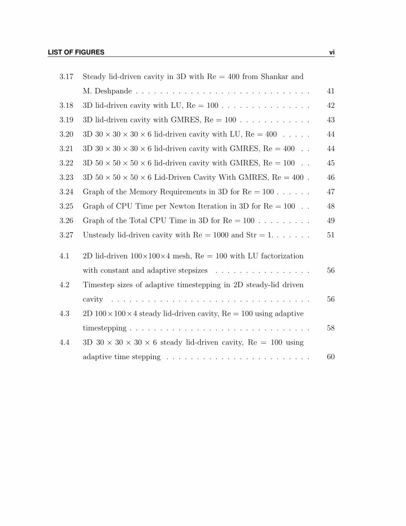
List of figures v
List of Tables vii
1 Introduction 1
1.1 Navier–Stokes Equations . . . . . . . . . . . . . . . . . . . . . . 2
1.2 Discretization with Finite Element Method . . . . . . . . . . . . 4
2 Iterative Methods Used for Solving the Discretized Navier–Stokes
Equations 8
2.1 Time Stepping Schemes . . . . . . . . . . . . . . . . . . . . . . . 9
2.2 Iterative Solvers . . . . . . . . . . . . . . . . . . . . . . . . . . . 10
2.3 Preconditioning . . . . . . . . . . . . . . . . . . . . . . . . . . . 15
2.4 Portable, Extensible Toolkit for Scientific Computation (PETSC) 18
3 Comparison of Iterative Methods 19
3.1 Results for a 2D Steady Lid-driven Cavity . . . . . . . . . . . . . 19
3.2 Results for a 3D Steady Lid-driven Cavity . . . . . . . . . . . . . 38
3.3 Results for a 2D Pulsating Lid-driven Cavity . . . . . . . . . . . 49
iii
CONTENTS iv
4 Adaptive Time Stepping 52
4.1 Outline of the Method . . . . . . . . . . . . . . . . . . . . . . . . 52
4.2 Results of Adaptive Time Stepping on the 2D Lid-driven Cavity 54
4.3 Results of Adaptive Time Stepping on the 3D Lid-driven Cavity 57
5 Conclusion 61
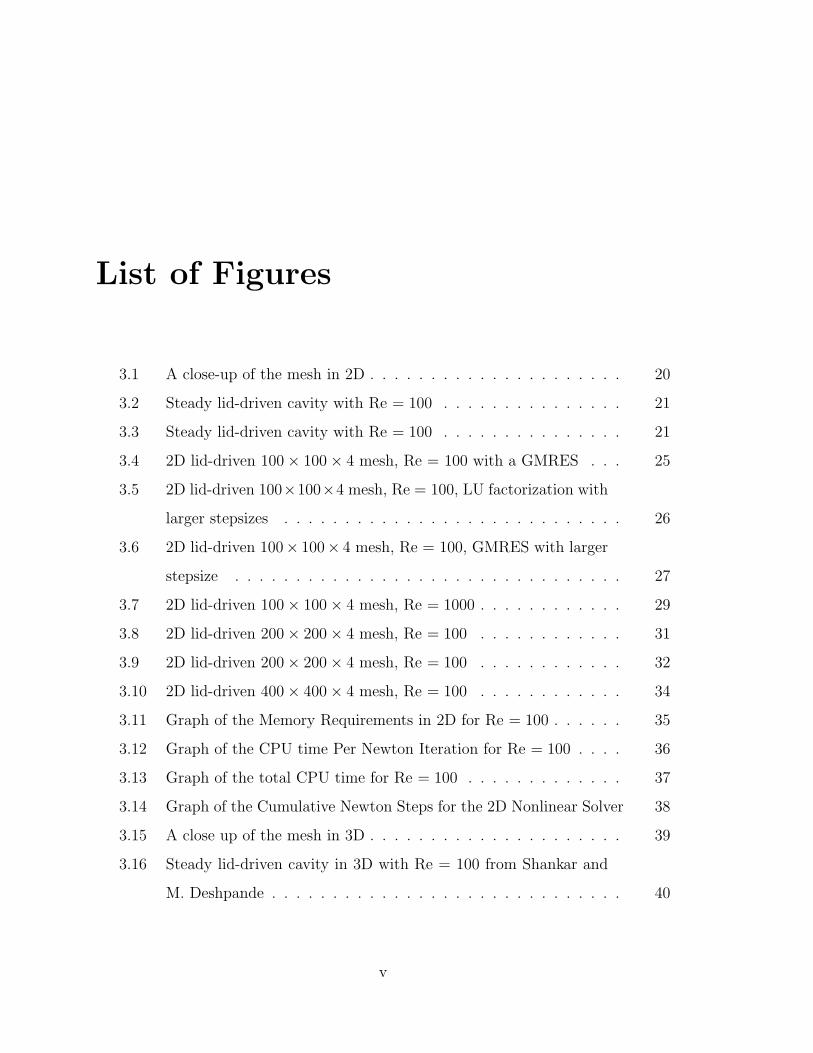
List of Figures
3.1 A close-up of the mesh in 2D . . . . . . . . . . . . . . . . . . . . . 20
3.2 Steady lid-driven cavity with Re = 100 . . . . . . . . . . . . . . . 21
3.3 Steady lid-driven cavity with Re = 100 . . . . . . . . . . . . . . . 21
3.4 2D lid-driven 100× 100× 4 mesh, Re = 100 with a GMRES . . . 25
3.5 2D lid-driven 100×100×4 mesh, Re = 100, LU factorization with
larger stepsizes . . . . . . . . . . . . . . . . . . . . . . . . . . . . 26
3.6 2D lid-driven 100× 100× 4 mesh, Re = 100, GMRES with larger
stepsize . . . . . . . . . . . . . . . . . . . . . . . . . . . . . . . . 27
3.7 2D lid-driven 100× 100× 4 mesh, Re = 1000 . . . . . . . . . . . . 29
3.8 2D lid-driven 200× 200× 4 mesh, Re = 100 . . . . . . . . . . . . 31
3.9 2D lid-driven 200× 200× 4 mesh, Re = 100 . . . . . . . . . . . . 32
3.10 2D lid-driven 400× 400× 4 mesh, Re = 100 . . . . . . . . . . . . 34
3.11 Graph of the Memory Requirements in 2D for Re = 100 . . . . . . 35
3.12 Graph of the CPU time Per Newton Iteration for Re = 100 . . . . 36
3.13 Graph of the total CPU time for Re = 100 . . . . . . . . . . . . . 37
3.14 Graph of the Cumulative Newton Steps for the 2D Nonlinear Solver 38
3.15 A close up of the mesh in 3D . . . . . . . . . . . . . . . . . . . . . 39
3.16 Steady lid-driven cavity in 3D with Re = 100 from Shankar and
M. Deshpande . . . . . . . . . . . . . . . . . . . . . . . . . . . . . 40
v
LIST OF FIGURES vi
3.17 Steady lid-driven cavity in 3D with Re = 400 from Shankar and
M. Deshpande . . . . . . . . . . . . . . . . . . . . . . . . . . . . . 41
3.18 3D lid-driven cavity with LU, Re = 100 . . . . . . . . . . . . . . . 42
3.19 3D lid-driven cavity with GMRES, Re = 100 . . . . . . . . . . . . 43
3.20 3D 30× 30× 30× 6 lid-driven cavity with LU, Re = 400 . . . . . 44
3.21 3D 30× 30× 30× 6 lid-driven cavity with GMRES, Re = 400 . . 44
3.22 3D 50× 50× 50× 6 lid-driven cavity with GMRES, Re = 100 . . 45
3.23 3D 50× 50× 50× 6 Lid-Driven Cavity With GMRES, Re = 400 . 46
3.24 Graph of the Memory Requirements in 3D for Re = 100 . . . . . . 47
3.25 Graph of CPU Time per Newton Iteration in 3D for Re = 100 . . 48
3.26 Graph of the Total CPU Time in 3D for Re = 100 . . . . . . . . . 49
3.27 Unsteady lid-driven cavity with Re = 1000 and Str = 1. . . . . . . 51
4.1 2D lid-driven 100×100×4 mesh, Re = 100 with LU factorization
with constant and adaptive stepsizes . . . . . . . . . . . . . . . . 56
4.2 Timestep sizes of adaptive timestepping in 2D steady-lid driven
cavity . . . . . . . . . . . . . . . . . . . . . . . . . . . . . . . . . 56
4.3 2D 100×100×4 steady lid-driven cavity, Re = 100 using adaptive
timestepping . . . . . . . . . . . . . . . . . . . . . . . . . . . . . . 58
4.4 3D 30 × 30 × 30 × 6 steady lid-driven cavity, Re = 100 using
adaptive time stepping . . . . . . . . . . . . . . . . . . . . . . . . 60
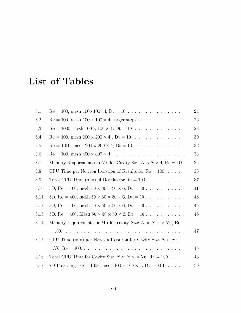
List of Tables
3.1 Re = 100, mesh 100×100×4, Dt = 10 . . . . . . . . . . . . . . . . 24
3.2 Re = 100, mesh 100× 100× 4, larger stepsizes . . . . . . . . . . . 26
3.3 Re = 1000, mesh 100× 100× 4, Dt = 10 . . . . . . . . . . . . . . 28
3.4 Re = 100, mesh 200× 200× 4 , Dt = 10 . . . . . . . . . . . . . . 30
3.5 Re = 1000, mesh 200× 200× 4, Dt = 10 . . . . . . . . . . . . . . 32
3.6 Re = 100, mesh 400× 400× 4 . . . . . . . . . . . . . . . . . . . . 33
3.7 Memory Requirements in Mb for Cavity Size N ×N × 4, Re = 100. 35
3.8 CPU Time per Newton Iteration of Results for Re = 100. . . . . . 36
3.9 Total CPU Time (min) of Results for Re = 100. . . . . . . . . . . 37
3.10 3D, Re = 100, mesh 30× 30× 30× 6, Dt = 10 . . . . . . . . . . . 41
3.11 3D, Re = 400, mesh 30× 30× 30× 6, Dt = 10 . . . . . . . . . . . 43
3.12 3D, Re = 100, mesh 50× 50× 50× 6, Dt = 10 . . . . . . . . . . . 45
3.13 3D, Re = 400, Mesh 50× 50× 50× 6, Dt = 10 . . . . . . . . . . . 46
3.14 Memory requirements in Mb for cavity Size N × N × ×N6, Re
= 100. . . . . . . . . . . . . . . . . . . . . . . . . . . . . . . . . . 47
3.15 CPU Time (min) per Newton Iteration for Cavity Size N ×N ×
×N6, Re = 100. . . . . . . . . . . . . . . . . . . . . . . . . . . . . 48
3.16 Total CPU Time for Cavity Size N ×N ××N6, Re = 100. . . . . 48
3.17 2D Pulsating, Re = 1000, mesh 100× 100× 4, Dt = 0.01 . . . . . 50
vii
LIST OF TABLES viii
4.1 Re = 100, mesh 100× 100× 4 , Adaptive Timestepping . . . . . . 55
4.2 Re = 100, mesh 30× 30× 30× 6 , Adaptive Timestepping . . . . 59
Chapter 1
Elementary Concepts
Numerical methods have a vast range of applications which include approximating
partial differential equations that appear in the study of fluid mechanics. The gov-
erning equations of motion in the study of fluids are the Navier–Stokes equations,
a system of partial differential equations due to Claude-Louis Navier and George
Gabriel Stokes. The problem of efficiently and accurately solving the Navier–Stokes
equations is not a simple process and is an on-going task that is being refined year
after year. The goal of this thesis is to analyze some of these methods in some simple
2D and 3D test cases. Simulating flows has many applications such as blood flow in
the circulatory system and air flow in the respiratory system just to name a few. A
relevant example would be to analyze the effects of installing a ventricular assist de-
vice, which acts as a mechanical pump for hearts that are too weak to pump the blood.
A first glance at the Navier–Stokes equations in their continuous form readily shows
difficulties, especially when the domain, boundary conditions and initial conditions
become complex. As we shall soon see, many methods have been derived to tackle this
problem with promising results. Discretization of the equations via a Finite Element
Method (FEM) aids in reducing them to a system of algebraic differential equations
1
1.1. Navier–Stokes Equations 2
and then an appropriate time stepping scheme can be chosen to further reduce our
problem to a system of nonlinear iterative equations. One can then linearize the
equations via a method such as Newton’s method. Once the equations have been
linearized methods like the generalized minimal residual method (GMRES), least
squares method or in the case of a symmetric Jacobian matrix, the conjugate gradi-
ent method (CG) or conjugate residual method (CR) may be used. In our case the
Navier–Stokes equations generate a non-symmetric Jacobian matrix which leaves us
with few choices for an iterative solver. GMRES is a common choice here. Even once
linearized, other tricks are required. One being the use of a preconditioner. Precon-
ditioners are used when the condition number of the linear system of equations is too
large. Generally, a preconditioner will not require many extra computations but will
speed up the convergence.
In this first chapter we will introduce the Navier-Stokes Equations in their continuous
form and outline the process of using a finite element method to reduce the equations
to a fully discretized system of nonlinear algebraic equations.
1.1 Navier–Stokes Equations
Given a flow problem in Rd we shall set u = (u1, . . . , ud)T to be the velocity vector of
the flow and p the pressure field. Let Ω ⊂ Rd be a bounded domain with boundary
Γ, then the Navier–Stokes equations for incompressible flow in their non-dimensional
form are
1.1. Navier–Stokes Equations 3
∂u
∂t+ u · ∇u+∇p− Re−1∆u = f in Ω,
∇ · u = 0 in Ω,
u = uΓ on Γ,
u(·, 0) = u0 in Ω.
(1.1.1)
The first equation is called the momentum equation, the second is the conservation of
mass and the third and fourth are the boundary and initial conditions, respectively.
The non-dimensional parameter Re represents the Reynolds number and is defined
as Re = V L/ν where V and L are the characteristic velocity and length of the flow,
respectively. The parameter ν is the kinematic viscosity, the function f is given and
represents a body force such as gravity, uΓ is the prescribed velocity on the boundary
Γ of the domain Ω and u0 is the initial velocity.
Now we want to state the Navier–Stokes equations in variational form. Let L2(Ω) be a
second order Lebesgue space on Ω. We define the Sobolev spaceH10 (Ω) = u ∈ L2(Ω) :
∂u ∈ L2(Ω), u = 0 on Γ and the Lebesgue space L20(Ω) = q ∈ L2 :
∫Ωq = 0.
We shall require test functions v ∈ [H10 (Ω)]d and q ∈ L2
0(Ω). We then multiply
the conservation of momentum and mass equations by v and q, respectively, and
integrate by parts over Ω yielding a variational form of the problem (1.1.1): Find
u ∈ w ∈ [H1(Ω)]d : w|Γ = u|Γ and p ∈ L2∫=0
(Ω) such that
d
dt(u, v) + c(u, u, v) + b(v, p) + a(u, v) = (f, v) for any v ∈ [H1
0 (Ω)]d,
b(u, q) = 0 for any q ∈ L20(Ω).
(1.1.2)
The above products are outlined in [7] and defined to be
(u, v) =
∫Ω
u · v dx, c(u, v, w) =∫
Ω(u · ∇v) · w dx,
b(q, v) = −∫
Ω
q∇ · v dx, a(u, v) = 1Re
∫Ω∇u : ∇v dx,
(1.1.3)
1.2. Discretization with Finite Element Method 4
where ∇u : ∇v =∑i,j
∂ui∂xj
∂vi∂xj
.
The Navier–Stokes equations in their continuous form are of limited use until they
are fully discretized. For this, we use a Galerkin type finite element method (GFEM)
that will be discussed in the next section. The variational form of the Navier–Stokes
equations is our first bridge to this numerical approximation.
1.2 Discretization with Finite Element Method
To solve equations (1.1.1) we must use a finite element method for the velocity and
the pressure terms. In order to stabilize these elements a Streamline-Upwind Petrov
Galerkin / Pressure–Stabilized Petrov Galerkin (SUPG/PSPG) formulation is used.
A paper by P. Kjellgren [11] explains the need for the SUPG formulation saying that
the convective terms of the Navier–Stokes equations are the cause for some numerical
problems involving the appearance of oscillatory solutions and a means for stabilizing
these is with upwinding. Upwinding is a scheme that aids in properly simulating the
direction of propagation of a fluid flow. PSPG is required to bypass Brezzi–Babuska
conditions [4],[7]. In the following section we shall first see what is a mesh and how
to obtain the SUPG/PSPG formulation of (1.1.1). Following this we will obtain the
fully discretized Navier–Stokes equations using Galerkin’s method. For this let us
first define what is a mesh.
Definition 1.2.1 [4, p. 32][Mesh] Let Ω be a domain in Rd. A mesh is a union of
a finite number N of compact, connected, Lipschitz sets Km with non-empty interior
Km such that Km1≤m≤N forms a partition of Ω, i.e.,
Ω =N⋃m=1
Km and Km ∩ Kn = ∅ for m 6= n.
1.2. Discretization with Finite Element Method 5
Denote the mesh by Th where h = max1≤i≤N
diamKi
In practice, a mesh is generated from a reference finite element and a set of geomet-
ric transformations mapping the reference cell K to the rest of the mesh cells. Let
K ∈ Th be any cell in the mesh then the geometric transformation is typically denoted
by Tk : K → K. For our problem of discretizing the Navier–Stokes equations we shall
use a mesh consisting of triangles or tetrahedra, making a triangulation of the domain.
The SUPG/PSPG formulation is a Petrov–Galerkin formulation in which a weight
function is applied to all the terms in the Navier–Stokes equations. Let Th be a
triangulation of the domain Ω into elements K with diameter hk. We next define the
spaces of test functions for pressure and velocity as
Qh = qh|qh ∈ P 1h,
Vh = uh|uh ∈ [P 1h ]d, uh = ΠhuΓ on Γh,
Vh0 = vh|vh ∈ [P 1h ]d, vh = 0 on Γh,
where P 1h is the set of continuous P 1 finite elements on the mesh Th and Πh the
usual P 1 Lagrange interpolation operator. The SUPG/PSPG formulation of the
semi-discretized problem (1.1.1) is as follows: Find (uh, ph) ∈ Vh × Qh such that for
all (vh, qh) ∈ Vh0 ×Qh
ddt
(uh, vh) + b(uh, uh, vh) + a(uh, vh)− (∇ · vh, ph) + (qh,∇ · uh) + ST = (vh, f),
uh(·, 0) = Πhu0(·) in Ω.
(1.2.1)
The PSPG/SUPG stabilization term is given by
ST =∑Kh∈Th
∫Kh
(τSUPGuh · ∇vh + τPSPG∇qh) ·R(uh, ph) dx,
1.2. Discretization with Finite Element Method 6
where R(uh, ph) = ∂∂tuh+uh ·∇uh−ν∆uh+∇ph−f is the residual of the momentum
equation. The coefficients τSUPG and τPSPG are defined as
τSUPG := αuhk
2‖uh‖ξ, τPSPG := αp
hk2‖uh‖
ξ,
where ξ is a function of the element’s Reynolds number RK = 0.5||uh||hk
νand is given
by ξ(RK) = max 0,min RK
3, 1. The typical values for αu and αp are between 1
and 5.
We shall next use locally linear shape functions that are determined by the value at
the vertices of the triangle or tetrahedron. Essentially we are re-writing our problem
in a new basis, that of our local shape functions. This will simplify the calculations
needed to solve for the terms in the variational form of the Navier–Stokes equations
(1.1.2). The GFEM uses P 1 local shape functions, say θ1, . . . , θn for the velocity
and ψ1, . . . , ψm for the pressure terms, and estimates u by uh with uh =n∑j=1
Ujθj,
with Uj = (Uj1, . . . , Ujd] ∈ Rd and similarly estimates p by ph with ph =m∑j=1
Pjψj with
Pj ∈ R. We shall introduce two new vectors, U = [U1, . . . , Un]T and P = [P1, . . . , Pj]T .
The next step is to replace these estimates into (1.2.1). Now since the test function
vh is arbitrary in Vh0 we can choose it to be one of our shape functions, say θ = θi,
i = 1, . . . , n for each velocity component. Let us look at what happens to our first
product (uh, vh) =∫
Ωuh · vh dx:∫
Ω
uh · vh dx =
∫Ω
( n∑j=1
Ujθj · θ)dx
=n∑j=1
∫Ω
Ujθjθi dx, where i = 1, . . . , n
= U1
∫Ω
θ1θi dx+ · · ·+ Un
∫Ω
θnθi dx, where i = 1, . . . , n
= MijU
where Mij is an nu × nu matrix whose ijth entry is
∫Ω
θiθj dx
1.2. Discretization with Finite Element Method 7
We shall set qh = 0 and let U represent the time derivative. Applying similar tech-
niques as above to the other terms in equation (1.2.1) we obtain the following dis-
cretized form as in [11]:
MU +N(U) +KU −BTP = F,
BU = 0,(1.2.2)
where the matrices M , N , K, BT and B are the mass, convection, diffusion, gradient
and divergence matrices, respectively, and F is a vector representing an external force.
The ijth entries of the matrices corresponding to those just mentioned are defined as
Mij =
∫Ω
θi · θj dx,
Nij =
∫Ω
(uh · ∇θi) · θj dx
Kij =
∫Ω
∇(θi) : ∇(θj) dx,
BTij =
∫Ω
ψjdiv(θi) dx.
From the variational form we used a SUPG/PSPG finite element method to obtain
equation (1.2.2); however there is still a time derivative in this equation that needs
to be dealt with. This is where numerical methods in ordinary differential equations
(ODE’s) will be useful since our only independent variable is now that of time. There
are several different time-stepping schemes that can be used; Gresho[6] and [7], pro-
vides very good resources for instance, for choosing appropriate numerical methods
when dealing with PDE’s and outlines some good choices for dealing with advection-
diffusion problems such as the Navier–Stokes problem. The methods that were used
in this research will be outlined in Chapter 2.
Chapter 2
Iterative Methods Used for Solving
the Discretized Navier–Stokes
Equations
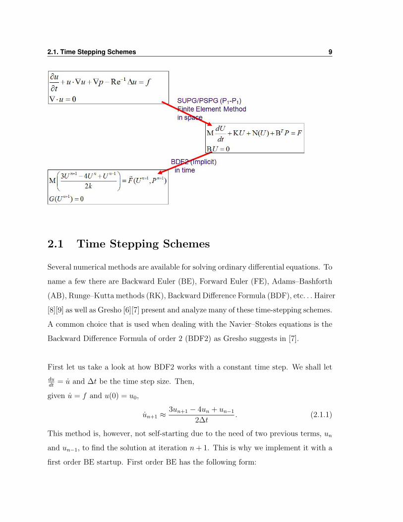
Now that we have used the FEM in space, chapter two will introduce the numerical
methods used to approximate the time derivative as well as the iterative methods
used to solve the fully discretized Navier–Stokes equations. The following diagram
shows a skeleton of the discretization process.
8
2.1. Time Stepping Schemes 9
2.1 Time Stepping Schemes
Several numerical methods are available for solving ordinary differential equations. To
name a few there are Backward Euler (BE), Forward Euler (FE), Adams–Bashforth
(AB), Runge–Kutta methods (RK), Backward Difference Formula (BDF), etc. . .Hairer
[8][9] as well as Gresho [6][7] present and analyze many of these time-stepping schemes.
A common choice that is used when dealing with the Navier–Stokes equations is the
Backward Difference Formula of order 2 (BDF2) as Gresho suggests in [7].
First let us take a look at how BDF2 works with a constant time step. We shall let
dudt
= u and ∆t be the time step size. Then,
given u = f and u(0) = u0,
un+1 ≈3un+1 − 4un + un−1
2∆t. (2.1.1)
This method is, however, not self-starting due to the need of two previous terms, un
and un−1, to find the solution at iteration n+ 1. This is why we implement it with a
first order BE startup. First order BE has the following form:
2.2. Iterative Solvers 10
un+1 ≈un+1 − un
∆t. (2.1.2)
BE is used with u0 to get u1 and then after this first step we have enough values to
use BDF2 for all remaining steps. If we apply BDF2 to the Navier–Stokes equations
we have the following implicit scheme for a difference algebraic equation (DAE):
M
(3Un+1 − 4Un + Un−1
2∆t
)+KUn+1 +N(Un+1)Un+1 −BTPn+1 = Fn,
BUn+1 = 0,
(2.1.3)
that needs to be solved at each time step.
2.2 Iterative Solvers
Iterative solvers are essential tools for solving large systems of algebraic equations like
the discretized Navier–Stokes equations. Many methods have been developed like de-
scent methods, gradient methods and Newton’s method. Many of these methods are
described in Saad’s book [12]. Due to the nonlinearity of the discretized Navier–
Stokes equations, Newton’s method is a common starting point as it transforms the
problem into a linear system. This is the method that will be used in this thesis.
Given the nonlinear function G(U) = 0 and an initial guess of the solution U0, the
general step for a Newton iteration is
[DG(Un)]δU = −G(Un)
Un+1 = Un + δU.(2.2.1)
From equation (2.1.3) we shall set
G(Un+1, Pn+1) =
M(
3Un+1−4Un+Un−1
2∆t
)+KUn+1 +N(Un+1) +BTPn+1 − Fn
BUn+1
.
2.2. Iterative Solvers 11
Applying Newton’s method to G yields[(3
2∆tM +K +DN(Un)
)δUn+1 −BT δPn+1
]Un+1 = G(Un),
BδUn+1 = 0,
(2.2.2)
where Un+1 = Un + δUn+1 and Pn+1 = Pn + δPn+1.
Now that the system has been linearized we must next choose an appropriate itera-
tive solver. In PETSC there are few options for this choice as the matrix obtained in
(2.2.2) is non-symmetric. The method available that best applies to the discretized
Navier–Stokes equations is the Generalized Minimal Residual Method (GMRES). It
is a generalization of the conjugate gradient algorithm as in [4, p. 405] and [12, p.
144–169]. In order to understand how GMRES works we need first to understand
projection-based iterative methods.
Before looking at the iterative methods let us quickly observe a direct method com-
monly used called LU factorization. Consider the system Ax = b. The first step is to
use Gaussian elimination to re-write the matrix A in the form
A = LU
where L and U are lower and upper triangular matrices, respectively. Now there are
two steps to solve our linear system:
(i) Solve Lx′ = b,
(ii) Solve Ux = x′.
For stability, pivoting needs to be used. Efficient as this method may be at getting ac-
curate solutions, the cost (number of operations) of using such a method for a system
of order n can be up to the order n3 if A is dense and this is due to the work involved
in getting the LU decomposition in the first place. The cost of solving the lower and
upper triangular systems can be up to the order n2 when A is dense. Sometimes an
2.2. Iterative Solvers 12
iterative method may be much more efficient though potentially less accurate.
Now consider the system Ax = b and assume A is non-singular. Let v ∈ Rn be an
approximation to the solution x. We will denote the error by e(v) = x − v and the
residual by r(v) = b− Av. Now we need two subspaces, K and L of Rn of the same
dimension. We shall try to improve the approximate solution v as in [4, p.402], by a
vector w that solves the problemSeek w ∈ v +K such that r(w)⊥L
. (2.2.3)
Since K and L have the same dimension and A is invertible, (2.2.3) is well posed [4].
Choosing L = AK we then seek the solution v of (2.2.3) that minimizes the residual
r(v) over the space v + K. There are many iterative methods based on the idea of
projection. The most commonly used are the conjugate gradient (CG) method and
GMRES. CG method applies to systems with symmetric, positive definite matrices
and GMRES applies to the general case.
In general, for an iterative projection method we are given u0 ∈ Rn; then at the mth
step of the iterative process we solve the problemSeek um ∈ u0 +Km such that r(um)⊥Lm
(2.2.4)
where Kmm≥1 and Lmm≥1 are two sequences of subspaces of Rn.
We next introduce the notion of Krylov space since Km can be taken as a space of
this type. Let r ∈ Rn, then the space
K(A, r, k) = spanr, Ar, . . . , Ak−1r
is called a Krylov space of order k generated by r and associated with the matrix
A. Arnoldi’s algorithm is one way of constructing an orthonormal basis for our space
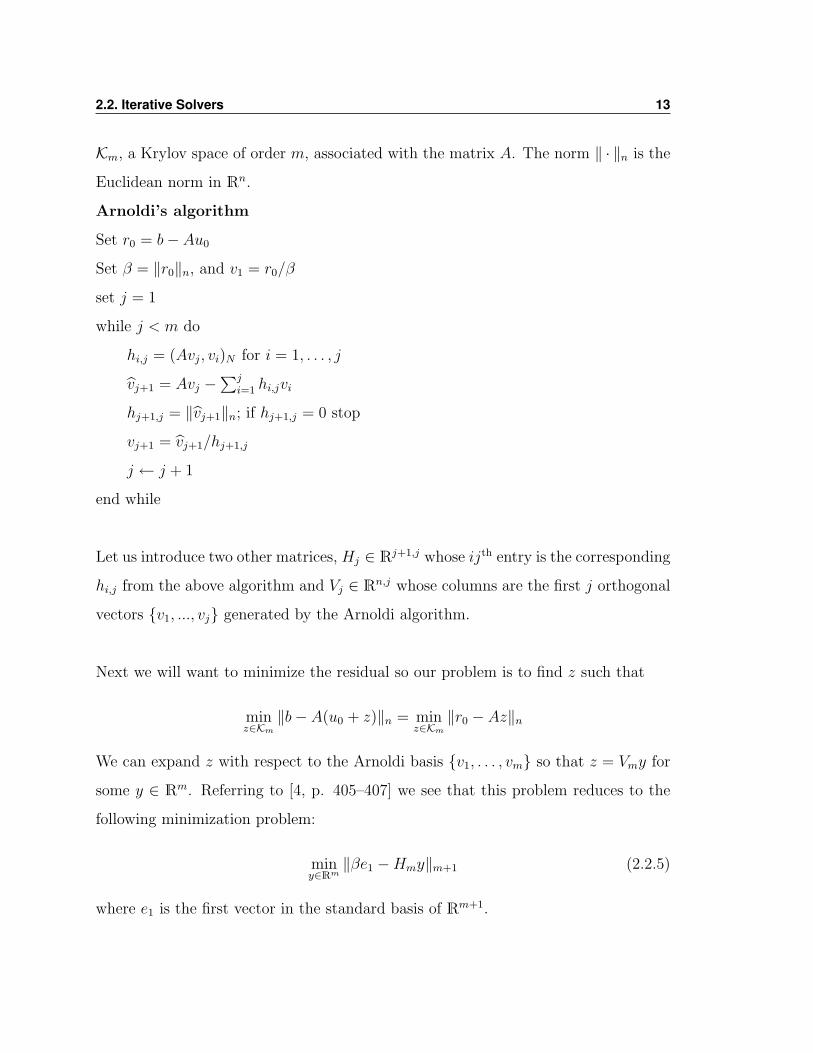
2.2. Iterative Solvers 13
Km, a Krylov space of order m, associated with the matrix A. The norm ‖ · ‖n is the
Euclidean norm in Rn.
Arnoldi’s algorithm
Set r0 = b− Au0
Set β = ‖r0‖n, and v1 = r0/β
set j = 1
while j < m do
hi,j = (Avj, vi)N for i = 1, . . . , j
vj+1 = Avj −∑j
i=1 hi,jvi
hj+1,j = ‖vj+1‖n; if hj+1,j = 0 stop
vj+1 = vj+1/hj+1,j
j ← j + 1
end while
Let us introduce two other matrices, Hj ∈ Rj+1,j whose ijth entry is the corresponding
hi,j from the above algorithm and Vj ∈ Rn,j whose columns are the first j orthogonal
vectors v1, ..., vj generated by the Arnoldi algorithm.
Next we will want to minimize the residual so our problem is to find z such that
minz∈Km
‖b− A(u0 + z)‖n = minz∈Km
‖r0 − Az‖n
We can expand z with respect to the Arnoldi basis v1, . . . , vm so that z = Vmy for
some y ∈ Rm. Referring to [4, p. 405–407] we see that this problem reduces to the
following minimization problem:
miny∈Rm
‖βe1 −Hmy‖m+1 (2.2.5)
where e1 is the first vector in the standard basis of Rm+1.
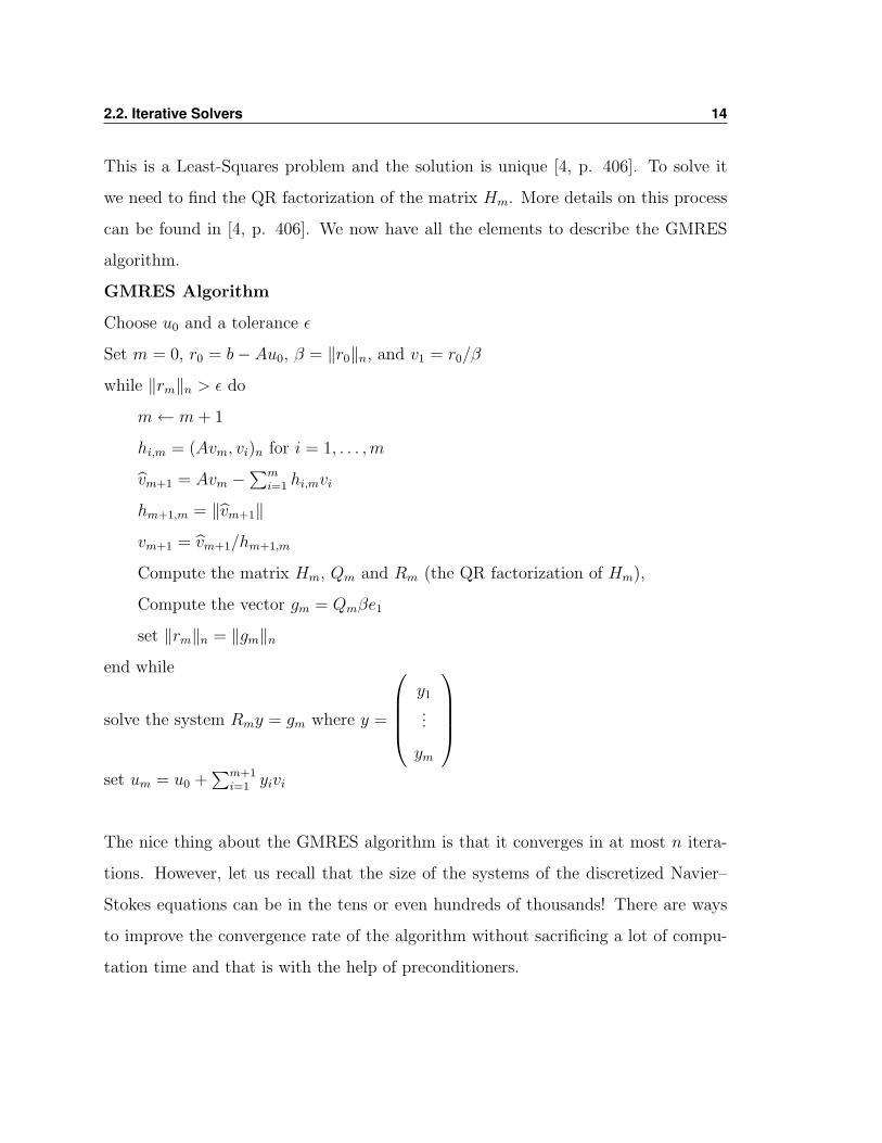
2.2. Iterative Solvers 14
This is a Least-Squares problem and the solution is unique [4, p. 406]. To solve it
we need to find the QR factorization of the matrix Hm. More details on this process
can be found in [4, p. 406]. We now have all the elements to describe the GMRES
algorithm.
GMRES Algorithm
Choose u0 and a tolerance ε
Set m = 0, r0 = b− Au0, β = ‖r0‖n, and v1 = r0/β
while ‖rm‖n > ε do
m← m+ 1
hi,m = (Avm, vi)n for i = 1, . . . ,m
vm+1 = Avm −∑m
i=1 hi,mvi
hm+1,m = ‖vm+1‖
vm+1 = vm+1/hm+1,m
Compute the matrix Hm, Qm and Rm (the QR factorization of Hm),
Compute the vector gm = Qmβe1
set ‖rm‖n = ‖gm‖nend while
solve the system Rmy = gm where y =
y1
...
ym
set um = u0 +
∑m+1i=1 yivi
The nice thing about the GMRES algorithm is that it converges in at most n itera-
tions. However, let us recall that the size of the systems of the discretized Navier–
Stokes equations can be in the tens or even hundreds of thousands! There are ways
to improve the convergence rate of the algorithm without sacrificing a lot of compu-
tation time and that is with the help of preconditioners.
2.3. Preconditioning 15
2.3 Preconditioning
This section deals with the concept of the condition number of a matrix A and its
effects on solving the linear system Ax = b. In essence, the condition number of a
matrix tells you how far away a matrix is from the set of singular matrices. Let us
define this so called condition number.
Definition 2.3.1 Let Z be an invertible n×n matrix. Its condition number is defined
as
κ(Z) = ‖Z‖n‖Z−1‖n.
We say that Z is ill-conditioned if κ(Z) 1.
It can easily be proved as in [4] that the condition number of a matrix is always
greater than or equal to 1 and also that when Z is symmetric κ(Z) =
∣∣∣∣λmax(Z)
λmin(Z)
∣∣∣∣where λmax(Z) and λmin(Z) are the largest and smallest eigenvalues of Z, respectively.
Since we are using numerical methods such as FEM and Newton’s method to get to
our linear system it is good to see what the effects of perturbation are on the system
Ax = b. If we look at the system A(x+ δx) = b+ δb it is easily shown that
‖δx‖n‖x‖n
≤ κ(A)‖δb‖n‖b‖n
,
and for the system (A+ δA)(x+ δx) = b that
‖δx‖n‖x+ δx‖n
≤ κ(A)‖δA‖n‖A‖n
.
These two estimates tell us that if A is ill-conditioned even slight perturbations in A or
b can lead to significant variations of the solution. The idea behind preconditioning
a system is to re-write Ax = b as a new linear system Ax = b where A is better
conditioned. One way of doing this is to take a non-singular matrix P and split it
into the form P = PLPR so that the systems PLy = a and PRz = c are easy and
inexpensive to solve. This P is going to be used as a split-preconditioner:
(P−1L AP−1
R )(PRx) = P−1L b. (2.3.1)
2.3. Preconditioning 16
Setting A = P−1L AP−1
R , x = PRx and b = P−1L b we have the new system Ax = b,
where A ideally has a lower condition number then A. This split preconditioner is
needed for symmetric matrices involving methods like CG in order to preserve the
symmetry of A but due to the fact that GMRES works for non-symmetric A, it is
more convenient and useful to simply use a left preconditioner or right preconditioner.
Let us consider a left preconditioned GMRES. The associated Krylov space would
then be
KPm = spanr0, (P−1)Ar0, . . . , (P
−1A)m−1r0.
Now by replacing A by P−1A and b by P−1b we can obtain a new preconditioned
algorithm for GMRES that would have a faster convergence rate than the original.
There are many ways you can precondition a linear system. Some of the more com-
mon preconditioners include the Incomplete LU factorization (ILU), Successive Over-
Relaxation (SOR) and Jacobi. Here we shall briefly explain the ILU, Jacobi and
block Jacobi preconditioners since we found these to be the most effective among
those tested while requiring a limited amount of memory to solve the Navier–Stokes
equations.
The basic idea of ILU is to form a simplified version of the LU factorization of the
matrix A, hence the name Incomplete LU factorization. If we are working with the
preconditioned system P−1Ax = P−1b where P is the preconditioning matrix, we will
want to form upper and lower triangular matrices, L and U , from A while maintaining
the sparsity pattern of A. That is, if the ijth entry of A is 0 then the ijth entry of
the matrix P = LU is also 0. The algorithm below is the basic scheme for an ILU
factorization and can also be found in [4, p. 413]. In Saad [12, p. 275] this algorithm
is also described in more detail and the author goes a step further to explain different
levels of filling. The algorithm below is known as ILU(0) since it has no levels of extra
2.3. Preconditioning 17
filling. The ILU(1) factorization has one level of filling and results from taking P to
be the zero pattern of the product LU of the factors L and U obtained from ILU(0).
For further levels of fill see [12].
ILU(0) Factorization Algorithm
for i = 2, ..., n do
for k = 1, ..., i− 1 do
if Aik 6= 0 then
Aik ← Aik/Akk
for j = k + 1, ..., n do
if Aij 6= 0 then
Aij ← Aij − AikAkjend if
end or
end if
end for
end for
The Jacobi preconditioner is one of the simplest ones; it is simply a diagonal ma-
trix whose elements are precisely those of the matrix of the system in question. For
the system P−1Ax = P−1b, P = D where D is the diagonal matrix just described.
The block Jacobi preconditioner is a block diagonal matrix and in the PETSC doc-
umentation [1] it uses the ILU method to fill in each individual block and the blocks
themselves can be taken to be of any size desired.
2.4. Portable, Extensible Toolkit for Scientific Computation (PETSC) 18
2.4 Portable, Extensible Toolkit for Scientific Com-
putation (PETSC)
PETSC is a suite of data structures and routines adapted for calculations of solutions
of partial differential equations. It is intended for large-scale projects and features
many libraries providing linear and nonlinear equations solvers that can be used in
conjunction with C, C++, Fortran and Python [1]. PETSC provides routines for solv-
ing the linear and nonlinear components of an algebraic differential equation like the
one derived in (1.2.2). The Scalable Nonlinear Equations solver (SNES) gives the user
access to Newton-based methods for solving nonlinear algebraic differential equations
such as equation (1.2.2) derived in section 1.2. Once the equation has been linearized
via the SNES the scalable linear equations solver (KSP) will provide Krylov subspace
based iterative methods. It is within these two interfaces that the user can specify
the type of iterative solver and precondtioners to use. A useful linear solver provided
by KSP is the Generalized Minimal Residual (GMRES) method. It is appropriate
for large sparse matrices that are non-symmetric as in the case of the discretized
Navier–Stokes equations. KSP also offers many choices for a preconditioner. The
list of available preconditioners includes Jacobi, Block Jacobi, ILU, ILU(n) and Suc-
cessive Over-Relaxation (SOR). Among the many types of convergence tests PETSC
offers, there are three in particular used for the SNES and KSP solvers, stol, atol
and rtol. One can declare convergence when the norm of the change in the solution
between successive iterations is less then some tolerance, stol. The tolerance atol is
the absolute size of the norm and rtol is the relative decrease of the absolute size of
the norm. It is also possible to bypass these convergence tests and specify a given
number of Newton or linear solver iterations.
Chapter 3
Comparison of Iterative Methods
In this chapter we will compare the performance of the iterative solver GMRES used
with preconditioners presented in Chapter 2 using three test cases:
i) a 2D steady lid-driven cavity
ii) a 2D pulsating lid-driven cavity
iii) a 3D steady lid-driven cavity.
3.1 Results for a 2D Steady Lid-driven Cavity
In this section I will present several results obtained on a simple 2D square lid-driven
cavity. This is a well-documented case and the benchmark solution used for compari-
son will be that of Ghia and Ghia [5]. Let us first discuss the domain of the test case.
It is the unit square cavity (0, 1) × (0, 1) with upper horizontal boundary called the
lid which is put into motion using the boundary condition u(x, 1, t) = (U(t), 0) where
U(t) is a prescribed function. For the steady lid-driven case U(t) = 1. All other sides
of the cavity (walls) are set to have a no-slip boundary condition which means that
u = 0 on the walls. The characteristic length and velocity are L = 1 and V = 1,
19
3.1. Results for a 2D Steady Lid-driven Cavity 20
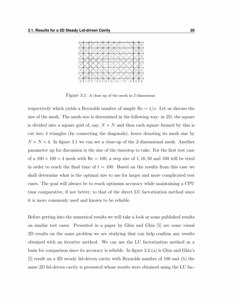
Figure 3.1: A close up of the mesh in 2 dimensions
respectively which yields a Reynolds number of simply Re = 1/ν. Let us discuss the
size of the mesh. The mesh size is determined in the following way: in 2D, the square
is divided into a square grid of, say, N × N and then each square formed by this is
cut into 4 triangles (by connecting the diagonals), hence denoting its mesh size by
N × N × 4. In figure 3.1 we can see a close-up of the 2-dimensional mesh. Another
parameter up for discussion is the size of the timestep to take. For the first test case
of a 100× 100× 4 mesh with Re = 100, a step size of 1, 10, 50 and 100 will be tried
in order to reach the final time of t = 100. Based on the results from this case we
shall determine what is the optimal size to use for larger and more complicated test
cases. The goal will always be to reach optimum accuracy while maintaining a CPU
time comparative, if not better, to that of the direct LU factorization method since
it is more commonly used and known to be reliable.
Before getting into the numerical results we will take a look at some published results
on similar test cases. Presented in a paper by Ghia and Ghia [5] are some visual
2D results on the same problem we are studying that can help confirm any results
obtained with an iterative method. We can use the LU factorization method as a
basis for comparison since its accuracy is reliable. In figure 3.2 (a) is Ghia and Ghia’s
[5] result on a 2D steady lid-driven cavity with Reynolds number of 100 and (b) the
same 2D lid-driven cavity is presented whose results were obtained using the LU fac-
3.1. Results for a 2D Steady Lid-driven Cavity 21
(a) (b)
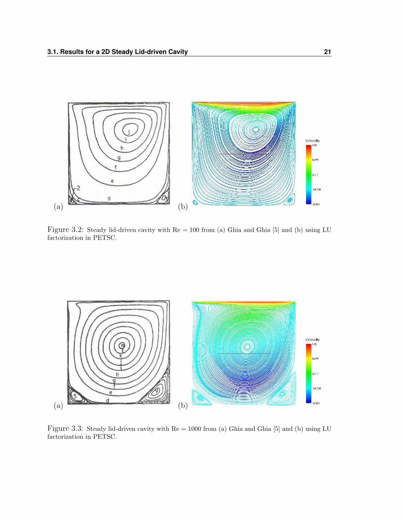
Figure 3.2: Steady lid-driven cavity with Re = 100 from (a) Ghia and Ghia [5] and (b) using LUfactorization in PETSC.
(a) (b)
Figure 3.3: Steady lid-driven cavity with Re = 1000 from (a) Ghia and Ghia [5] and (b) using LUfactorization in PETSC.
3.1. Results for a 2D Steady Lid-driven Cavity 22
torization in PETSC. Similarly in figure 3.3(a) is Ghia and Ghia’s result on a 2D
steady lid-driven cavity with Reynolds number of 1000 and (b) the results obtained
with the LU factorization in PETSC.
When experimenting with solvers it is good to look at the locations of vortices and
the prominent curves in the streamlines in order to have a good idea how well the
solvers are working. At a Reynolds number of 100 we see that the two vortices in the
bottom corners are much smaller than those of the case when the Reynolds number
is 1000. Also the location of the main vortex near the center is higher and to the
right at Re = 100 and at Re = 1000 it is moving its way closer to the center. One
other thing to note is the curve in the streamlines going towards the top left corner.
The lid of the cavity is moving in the positive x-direction and so this is pushing the
streamlines and forcing them to have a slight curve that becomes more evident in the
Re = 1000 case, as in agreement with remarks from Ghia and Ghia [5].
Now let us look at the numerical results on the 2D steady lid-driven test case with
the iterative solver GMRES. The options that are going to be varied in the test
cases are the types of preconditioners (PC type) used, the number of linear iterations
(KSPits), the number of nonlinear iterations (SNESits) and the stepsize. The CPU
time, memory used and the norm of the residuals (KSPres and SNESres) at the final
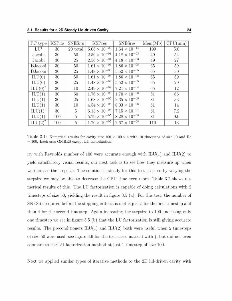
timestep are recorded at the end of each trial. A summary of this data for a test
case with mesh size 100 × 100 × 4 and Reynolds number Re = 100 is given in table
3.1. The first line shows the efficiency of the LU factorization. We can see that it
yields high accuracy using only about 5 minutes of CPU time; however, it is the
method that requires the largest amount of memory at 199 Mb. The total number of
Newton iterations required for this test case was 20 as we allowed PETSC to use its
default stopping criteria so that each timestep yields a different number of iterations
depending on the norms of the linear and nonlinear residuals. The default relative
3.1. Results for a 2D Steady Lid-driven Cavity 23
tolerance for the SNES iterations in PETSC is 1 × 10−08. This means that when
the ratio of two consecutive Newton iterations becomes equal to or smaller than this
tolerance, we shall stop the iteration process. In this first case the average number of
Newton iterations required to perform the LU factorization was about 4 per timestep.
When applying the iterative methods we started by using the preconditioner with the
smallest memory requirement, the Jacobi preconditioner. It only requires about 49
Mb of memory; however it yields poor results and the norms of the residuals are not
small enough to obtain a solution similar to Ghia’s or that of the LU factorization.
The Block Jacobi and the ILU(0) worked at the same efficiency. This is because the
Block Jacobi preconditioner uses ILU(0) to fill its entries at the block level. In all
following test cases, Block Jacobi will be excluded as it yields identical results to that
of ILU(0). When using ILU(0) we can see that the memory required to store the
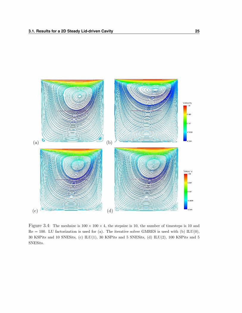
systems of equations has grown to about 65 Mb. Figure 3.4 shows the pictures for
the four tests from table 3.1 that have a †. We want to be able to see how the results
compare to (a) LU factorization so in figure (b) we have the case when ILU(0) is used
with 30 KSPits and 10 SNESits since we finally obtained a result that is comparable
in CPU time to that of LU factorization taking only 12 minutes to resolve (LU took
only 5 minutes). In (c) we have the case when ILU(1) is used with 30 KSPits and 5
SNESits are used. The memory is getting higher for this case using up 81Mb but is
still significantly lower than the 199 Mb required for LU. The residuals are getting
smaller with this preconditioner and since fewer SNESits were required to perform
the calculations, the CPU time diminished from that of the ILU(0) case to about 7.2
minutes. The last figure (d) is the result obtained with the ILU(2) preconditioner.
This one requires 110 Mb of memory but yields the smallest residuals of all the other
preconditioners tried.
Since we have found that the iterative method GMRES on the 100 × 100 × 4 cav-
3.1. Results for a 2D Steady Lid-driven Cavity 24
PC type KSPits SNESits KSPres SNESres Mem(Mb) CPU(min)
LU† 30 20 total 6.08× 10⁻²⁰ 1.64× 10⁻¹⁴ 199 5.0Jacobi 30 50 2.56× 10−01 4.18× 10−03 49 54Jacobi 30 25 2.56× 10−01 4.18× 10−03 49 27
BJacobi 30 50 1.61× 10−05 1.86× 10−08 65 59BJacobi 30 25 1.48× 10−03 5.52× 10−05 65 30ILU(0) 30 50 1.61× 10−05 1.86× 10−08 65 59ILU(0) 30 25 1.48× 10−03 5.52× 10−05 65 29
ILU(0)† 30 10 2.49× 10−02 7.21× 10−04 65 12ILU(1) 30 50 1.76× 10−05 1.70× 10−08 81 66ILU(1) 30 25 1.68× 10−05 2.35× 10−08 81 33ILU(1) 30 10 4.54× 10−05 8.03× 10−08 81 14
ILU(1)† 30 5 6.13× 10−05 7.15× 10−07 81 7.2ILU(1) 100 5 5.79× 10−05 8.28× 10−08 81 9.0
ILU(2)† 100 5 1.76× 10−05 2.67× 10−08 110 13
Table 3.1: Numerical results for cavity size 100 × 100 × 4 with 10 timesteps of size 10 and Re= 100. Each uses GMRES except LU factorization.
ity with Reynolds number of 100 were accurate enough with ILU(1) and ILU(2) to
yield satisfactory visual results, our next task is to see how they measure up when
we increase the stepsize. The solution is steady for this test case, so by varying the
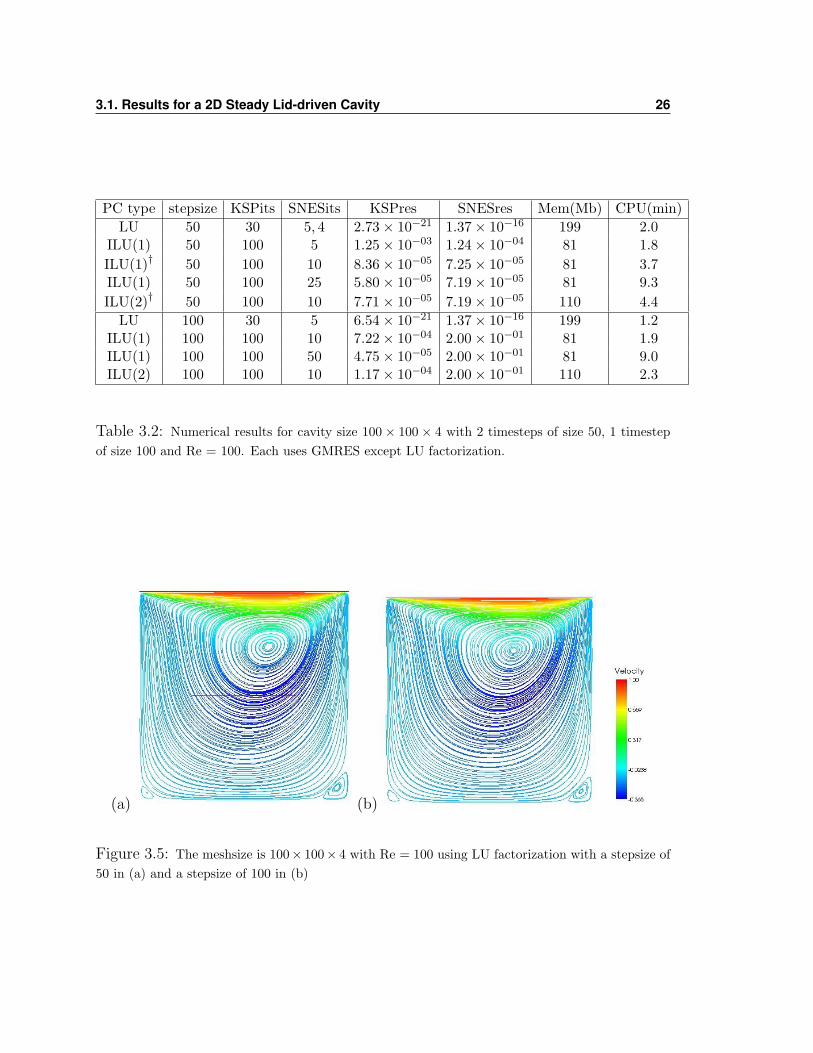
stepsize we may be able to decrease the CPU time even more. Table 3.2 shows nu-
merical results of this. The LU factorization is capable of doing calculations with 2
timesteps of size 50, yielding the result in figure 3.5 (a). For this test, the number of
SNESits required before the stopping criteria is met is just 5 for the first timestep and
than 4 for the second timestep. Again increasing the stepsize to 100 and using only
one timestep we see in figure 3.5 (b) that the LU factorization is still giving accurate
results. The preconditioners ILU(1) and ILU(2) both were useful when 2 timesteps
of size 50 were used, see figure 3.6 for the test cases marked with †, but did not even
compare to the LU factorization method at just 1 timestep of size 100.
Next we applied similar types of iterative methods to the 2D lid-driven cavity with
3.1. Results for a 2D Steady Lid-driven Cavity 25
(a) (b)
(c) (d)
Figure 3.4: The meshsize is 100 × 100 × 4, the stepsize is 10, the number of timesteps is 10 andRe = 100. LU factorization is used for (a). The iterative solver GMRES is used with (b) ILU(0),30 KSPits and 10 SNESits, (c) ILU(1), 30 KSPits and 5 SNESits, (d) ILU(2), 100 KSPits and 5SNESits.
3.1. Results for a 2D Steady Lid-driven Cavity 26
PC type stepsize KSPits SNESits KSPres SNESres Mem(Mb) CPU(min)LU 50 30 5, 4 2.73× 10⁻²¹ 1.37× 10⁻¹⁶ 199 2.0
ILU(1) 50 100 5 1.25× 10−03 1.24× 10−04 81 1.8ILU(1)† 50 100 10 8.36× 10−05 7.25× 10−05 81 3.7ILU(1) 50 100 25 5.80× 10−05 7.19× 10−05 81 9.3ILU(2)† 50 100 10 7.71× 10−05 7.19× 10−05 110 4.4
LU 100 30 5 6.54× 10⁻²¹ 1.37× 10⁻¹⁶ 199 1.2ILU(1) 100 100 10 7.22× 10−04 2.00× 10−01 81 1.9ILU(1) 100 100 50 4.75× 10−05 2.00× 10−01 81 9.0ILU(2) 100 100 10 1.17× 10−04 2.00× 10−01 110 2.3
Table 3.2: Numerical results for cavity size 100 × 100 × 4 with 2 timesteps of size 50, 1 timestepof size 100 and Re = 100. Each uses GMRES except LU factorization.
(a) (b)
Figure 3.5: The meshsize is 100× 100× 4 with Re = 100 using LU factorization with a stepsize of50 in (a) and a stepsize of 100 in (b)
3.1. Results for a 2D Steady Lid-driven Cavity 27
(a) (b)
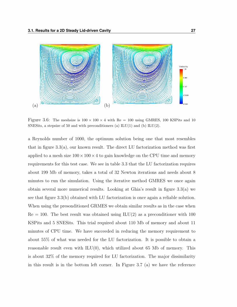
Figure 3.6: The meshsize is 100 × 100 × 4 with Re = 100 using GMRES, 100 KSPits and 10SNESits, a stepsize of 50 and with preconditioners (a) ILU(1) and (b) ILU(2).
a Reynolds number of 1000, the optimum solution being one that most resembles
that in figure 3.3(a), our known result. The direct LU factorization method was first
applied to a mesh size 100×100×4 to gain knowledge on the CPU time and memory
requirements for this test case. We see in table 3.3 that the LU factorization requires
about 199 Mb of memory, takes a total of 32 Newton iterations and needs about 8
minutes to run the simulation. Using the iterative method GMRES we once again
obtain several more numerical results. Looking at Ghia’s result in figure 3.3(a) we
see that figure 3.3(b) obtained with LU factorization is once again a reliable solution.
When using the presonditioned GRMES we obtain similar results as in the case when
Re = 100. The best result was obtained using ILU(2) as a preconditioner with 100
KSPits and 5 SNESits. This trial required about 110 Mb of memory and about 11
minutes of CPU time. We have succeeded in reducing the memory requirement to
about 55% of what was needed for the LU factorization. It is possible to obtain a
reasonable result even with ILU(0), which utilized about 65 Mb of memory. This
is about 32% of the memory required for LU factorization. The major dissimilarity
in this result is in the bottom left corner. In Figure 3.7 (a) we have the reference
3.1. Results for a 2D Steady Lid-driven Cavity 28
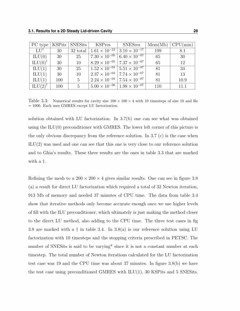
PC type KSPits SNESits KSPres SNESres Mem(Mb) CPU(min)
LU† 30 32 total 1.61× 10⁻²² 3.10× 10⁻¹⁷ 199 8.1ILU(0) 30 25 7.30× 10−05 6.40× 10−07 65 30
ILU(0)† 30 10 8.29× 10−05 7.37× 10−07 65 12ILU(1) 30 25 1.52× 10−04 5.51× 10−07 81 34ILU(1) 30 10 2.37× 10−04 7.74× 10−07 81 13ILU(1) 100 5 2.24× 10−04 7.54× 10−07 81 10.9
ILU(2)† 100 5 5.00× 10−06 1.98× 10−07 110 11.1
Table 3.3: Numerical results for cavity size 100 × 100 × 4 with 10 timesteps of size 10 and Re= 1000. Each uses GMRES except LU factorization.
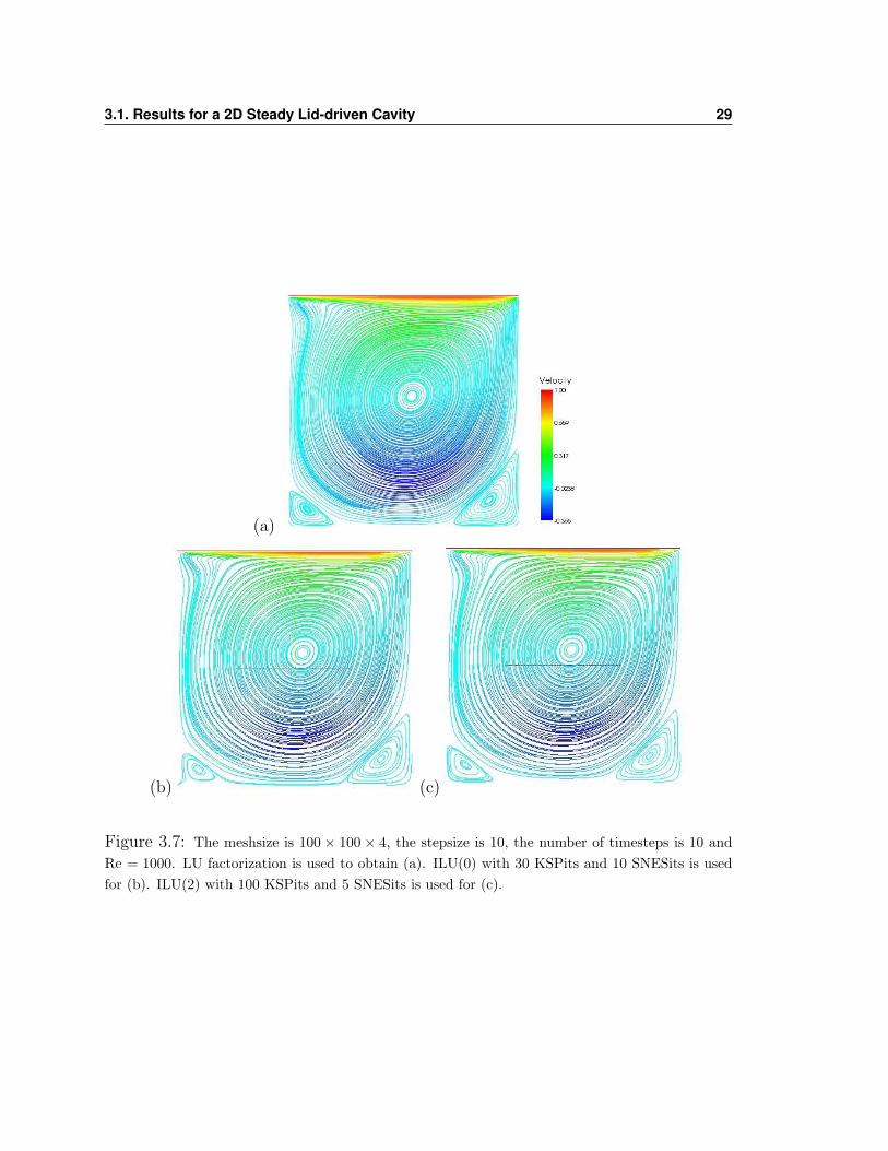
solution obtained with LU factorization. In 3.7(b) one can see what was obtained
using the ILU(0) preconditioner with GMRES. The lower left corner of this picture is
the only obvious discrepancy from the reference solution. In 3.7 (c) is the case when
ILU(2) was used and one can see that this one is very close to our reference solution
and to Ghia’s results. These three results are the ones in table 3.3 that are marked
with a †.
Refining the mesh to a 200× 200× 4 gives similar results. One can see in figure 3.8
(a) a result for direct LU factorization which required a total of 32 Newton iteration,
913 Mb of memory and needed 37 minutes of CPU time. The data from table 3.4
show that iterative methods only become accurate enough once we use higher levels
of fill with the ILU preconditioner, which ultimately is just making the method closer
to the direct LU method, also adding to the CPU time. The three test cases in fig
3.8 are marked with a † in table 3.4. In 3.8(a) is our reference solution using LU
factorization with 10 timesteps and the stopping criteria prescribed in PETSC. The
number of SNESits is said to be varying* since it is not a constant number at each
timestep. The total number of Newton iterations calculated for the LU factorization
test case was 19 and the CPU time was about 37 minutes. In figure 3.8(b) we have
the test case using preconditioned GMRES with ILU(1), 30 KSPits and 5 SNESits.
3.1. Results for a 2D Steady Lid-driven Cavity 29
(a)
(b) (c)
Figure 3.7: The meshsize is 100 × 100 × 4, the stepsize is 10, the number of timesteps is 10 andRe = 1000. LU factorization is used to obtain (a). ILU(0) with 30 KSPits and 10 SNESits is usedfor (b). ILU(2) with 100 KSPits and 5 SNESits is used for (c).
3.1. Results for a 2D Steady Lid-driven Cavity 30
PC type KSPits SNESits KSPres SNESres Mem(Mb) CPU(min)
LU† 30 19 total 8.69× 10⁻¹⁹ 8.77× 10⁻¹⁵ 913 37ILU(0) 30 25 3.80× 10−01 3.74× 10−03 235 201ILU(0) 30 10 3.80× 10−01 3.74× 10−03 235 81ILU(1) 30 25 2.74× 10−03 2.34× 10−05 313 255ILU(1) 30 10 1.75× 10−03 2.44× 10−05 313 102
ILU(1)† 30 5 8.63× 10−03 8.10× 10−05 313 43ILU(1) 100 5 1.11× 10−03 9.67× 10−06 313 54
ILU(2)† 100 5 4.47× 10−05 1.21× 10−07 426 70
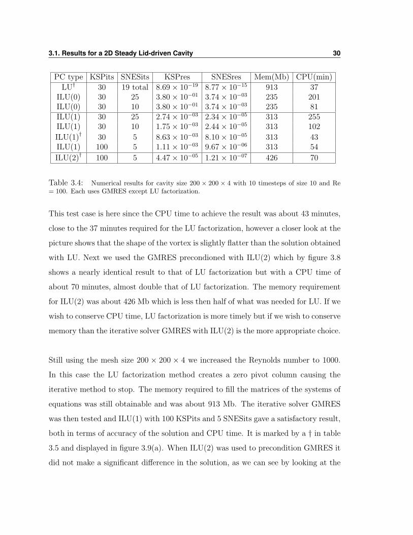
Table 3.4: Numerical results for cavity size 200 × 200 × 4 with 10 timesteps of size 10 and Re= 100. Each uses GMRES except LU factorization.
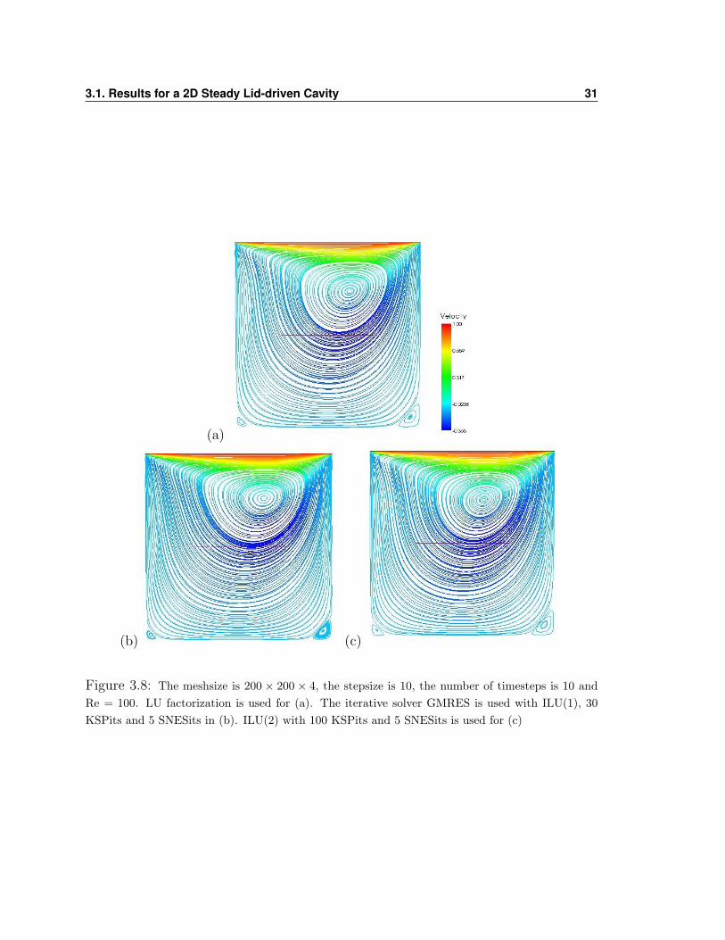
This test case is here since the CPU time to achieve the result was about 43 minutes,
close to the 37 minutes required for the LU factorization, however a closer look at the
picture shows that the shape of the vortex is slightly flatter than the solution obtained
with LU. Next we used the GMRES precondioned with ILU(2) which by figure 3.8
shows a nearly identical result to that of LU factorization but with a CPU time of
about 70 minutes, almost double that of LU factorization. The memory requirement
for ILU(2) was about 426 Mb which is less then half of what was needed for LU. If we
wish to conserve CPU time, LU factorization is more timely but if we wish to conserve
memory than the iterative solver GMRES with ILU(2) is the more appropriate choice.
Still using the mesh size 200 × 200 × 4 we increased the Reynolds number to 1000.
In this case the LU factorization method creates a zero pivot column causing the
iterative method to stop. The memory required to fill the matrices of the systems of
equations was still obtainable and was about 913 Mb. The iterative solver GMRES
was then tested and ILU(1) with 100 KSPits and 5 SNESits gave a satisfactory result,
both in terms of accuracy of the solution and CPU time. It is marked by a † in table
3.5 and displayed in figure 3.9(a). When ILU(2) was used to precondition GMRES it
did not make a significant difference in the solution, as we can see by looking at the
3.1. Results for a 2D Steady Lid-driven Cavity 31
(a)
(b) (c)
Figure 3.8: The meshsize is 200 × 200 × 4, the stepsize is 10, the number of timesteps is 10 andRe = 100. LU factorization is used for (a). The iterative solver GMRES is used with ILU(1), 30KSPits and 5 SNESits in (b). ILU(2) with 100 KSPits and 5 SNESits is used for (c)
3.1. Results for a 2D Steady Lid-driven Cavity 32
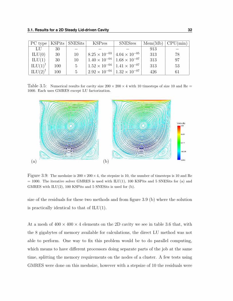
PC type KSPits SNESits KSPres SNESres Mem(Mb) CPU(min)LU 30 − − − 913 −
ILU(0) 30 10 8.25× 10−03 4.04× 10−05 313 78ILU(1) 30 10 1.40× 10−04 1.68× 10−07 313 97
ILU(1)† 100 5 1.52× 10−04 1.41× 10−07 313 53
ILU(2)† 100 5 2.92× 10−04 1.32× 10−07 426 61
Table 3.5: Numerical results for cavity size 200× 200× 4 with 10 timesteps of size 10 and Re =1000. Each uses GMRES except LU factorization.
(a) (b)
Figure 3.9: The meshsize is 200× 200× 4, the stepsize is 10, the number of timesteps is 10 and Re= 1000. The iterative solver GMRES is used with ILU(1), 100 KSPits and 5 SNESits for (a) andGMRES with ILU(2), 100 KSPits and 5 SNESits is used for (b).
size of the residuals for these two methods and from figure 3.9 (b) where the solution
is practically identical to that of ILU(1).
At a mesh of 400× 400× 4 elements on the 2D cavity we see in table 3.6 that, with
the 8 gigabytes of memory available for calculations, the direct LU method was not
able to perform. One way to fix this problem would be to do parallel computing,
which means to have different processors doing separate parts of the job at the same
time, splitting the memory requirements on the nodes of a cluster. A few tests using
GMRES were done on this meshsize, however with a stepsize of 10 the residuals were
3.1. Results for a 2D Steady Lid-driven Cavity 33
PC type stepsize KSPits SNESits KSPres SNESres Mem(Mb) CPU(min)LU 10 − − − − − −
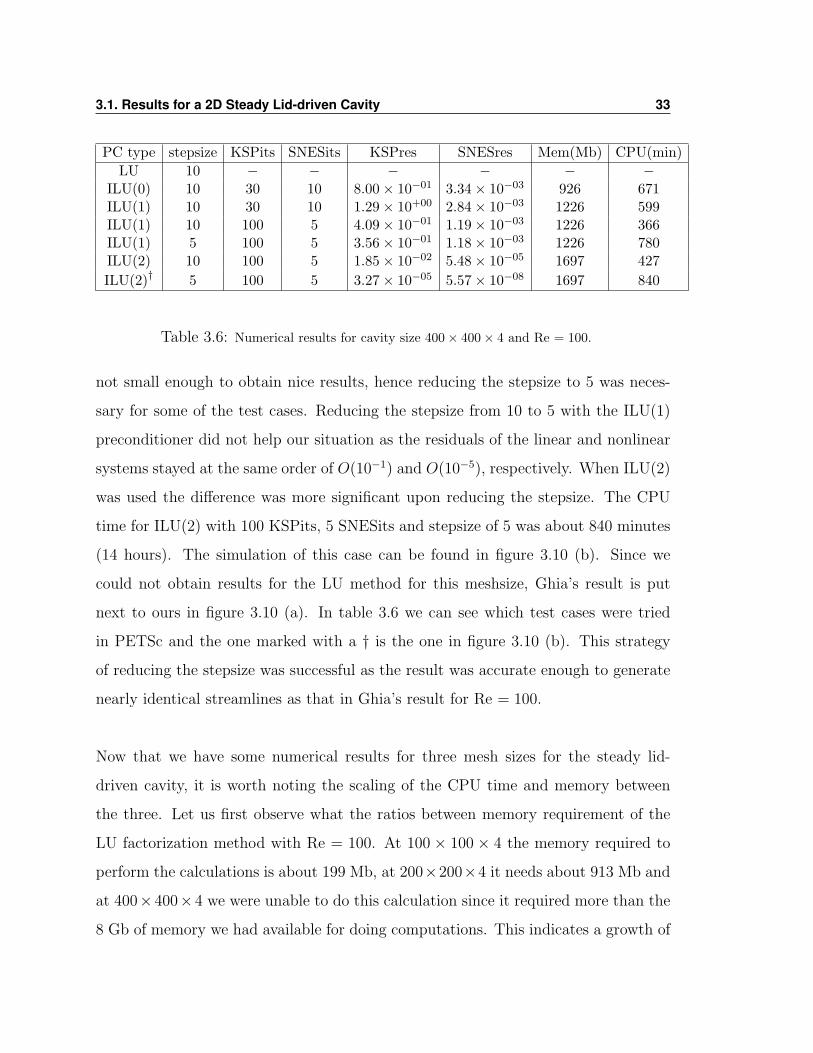
ILU(0) 10 30 10 8.00× 10−01 3.34× 10−03 926 671ILU(1) 10 30 10 1.29× 10+00 2.84× 10−03 1226 599ILU(1) 10 100 5 4.09× 10−01 1.19× 10−03 1226 366ILU(1) 5 100 5 3.56× 10−01 1.18× 10−03 1226 780ILU(2) 10 100 5 1.85× 10−02 5.48× 10−05 1697 427ILU(2)† 5 100 5 3.27× 10−05 5.57× 10−08 1697 840
Table 3.6: Numerical results for cavity size 400× 400× 4 and Re = 100.
not small enough to obtain nice results, hence reducing the stepsize to 5 was neces-
sary for some of the test cases. Reducing the stepsize from 10 to 5 with the ILU(1)
preconditioner did not help our situation as the residuals of the linear and nonlinear
systems stayed at the same order of O(10−1) and O(10−5), respectively. When ILU(2)
was used the difference was more significant upon reducing the stepsize. The CPU
time for ILU(2) with 100 KSPits, 5 SNESits and stepsize of 5 was about 840 minutes
(14 hours). The simulation of this case can be found in figure 3.10 (b). Since we
could not obtain results for the LU method for this meshsize, Ghia’s result is put
next to ours in figure 3.10 (a). In table 3.6 we can see which test cases were tried
in PETSc and the one marked with a † is the one in figure 3.10 (b). This strategy
of reducing the stepsize was successful as the result was accurate enough to generate
nearly identical streamlines as that in Ghia’s result for Re = 100.
Now that we have some numerical results for three mesh sizes for the steady lid-
driven cavity, it is worth noting the scaling of the CPU time and memory between
the three. Let us first observe what the ratios between memory requirement of the
LU factorization method with Re = 100. At 100 × 100 × 4 the memory required to
perform the calculations is about 199 Mb, at 200×200×4 it needs about 913 Mb and
at 400×400×4 we were unable to do this calculation since it required more than the
8 Gb of memory we had available for doing computations. This indicates a growth of
3.1. Results for a 2D Steady Lid-driven Cavity 34
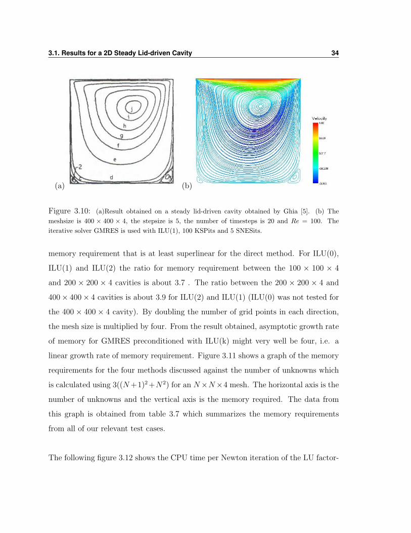
(a) (b)
Figure 3.10: (a)Result obtained on a steady lid-driven cavity obtained by Ghia [5]. (b) Themeshsize is 400 × 400 × 4, the stepsize is 5, the number of timesteps is 20 and Re = 100. Theiterative solver GMRES is used with ILU(1), 100 KSPits and 5 SNESits.
memory requirement that is at least superlinear for the direct method. For ILU(0),
ILU(1) and ILU(2) the ratio for memory requirement between the 100 × 100 × 4
and 200 × 200 × 4 cavities is about 3.7 . The ratio between the 200 × 200 × 4 and
400× 400× 4 cavities is about 3.9 for ILU(2) and ILU(1) (ILU(0) was not tested for
the 400 × 400 × 4 cavity). By doubling the number of grid points in each direction,
the mesh size is multiplied by four. From the result obtained, asymptotic growth rate
of memory for GMRES preconditioned with ILU(k) might very well be four, i.e. a
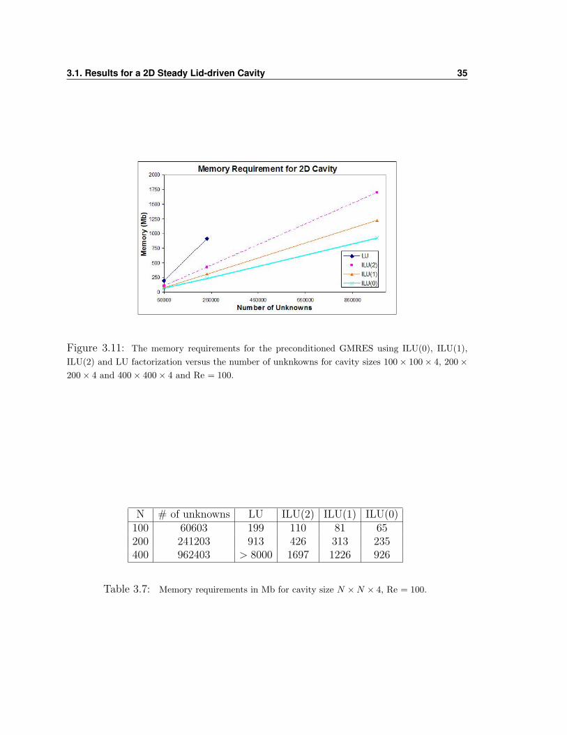
linear growth rate of memory requirement. Figure 3.11 shows a graph of the memory
requirements for the four methods discussed against the number of unknowns which
is calculated using 3((N+1)2 +N2) for an N×N×4 mesh. The horizontal axis is the
number of unknowns and the vertical axis is the memory required. The data from
this graph is obtained from table 3.7 which summarizes the memory requirements
from all of our relevant test cases.
The following figure 3.12 shows the CPU time per Newton iteration of the LU factor-
3.1. Results for a 2D Steady Lid-driven Cavity 35
Figure 3.11: The memory requirements for the preconditioned GMRES using ILU(0), ILU(1),ILU(2) and LU factorization versus the number of unknkowns for cavity sizes 100× 100× 4, 200×200× 4 and 400× 400× 4 and Re = 100.
N # of unknowns LU ILU(2) ILU(1) ILU(0)100 60603 199 110 81 65200 241203 913 426 313 235400 962403 > 8000 1697 1226 926
Table 3.7: Memory requirements in Mb for cavity size N ×N × 4, Re = 100.
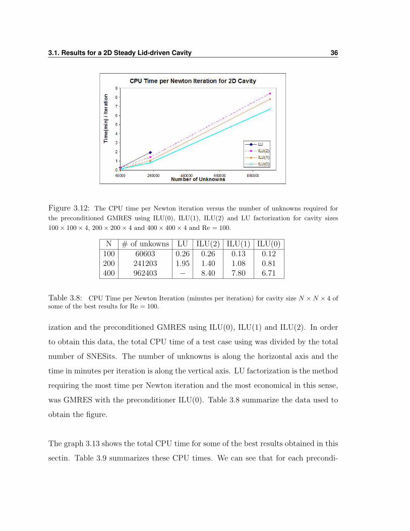
3.1. Results for a 2D Steady Lid-driven Cavity 36
Figure 3.12: The CPU time per Newton iteration versus the number of unknowns required forthe preconditioned GMRES using ILU(0), ILU(1), ILU(2) and LU factorization for cavity sizes100× 100× 4, 200× 200× 4 and 400× 400× 4 and Re = 100.
N # of unkowns LU ILU(2) ILU(1) ILU(0)100 60603 0.26 0.26 0.13 0.12200 241203 1.95 1.40 1.08 0.81400 962403 − 8.40 7.80 6.71
Table 3.8: CPU Time per Newton Iteration (minutes per iteration) for cavity size N ×N × 4 ofsome of the best results for Re = 100.
ization and the preconditioned GMRES using ILU(0), ILU(1) and ILU(2). In order
to obtain this data, the total CPU time of a test case using was divided by the total
number of SNESits. The number of unknowns is along the horizontal axis and the
time in minutes per iteration is along the vertical axis. LU factorization is the method
requiring the most time per Newton iteration and the most economical in this sense,
was GMRES with the preconditioner ILU(0). Table 3.8 summarize the data used to
obtain the figure.
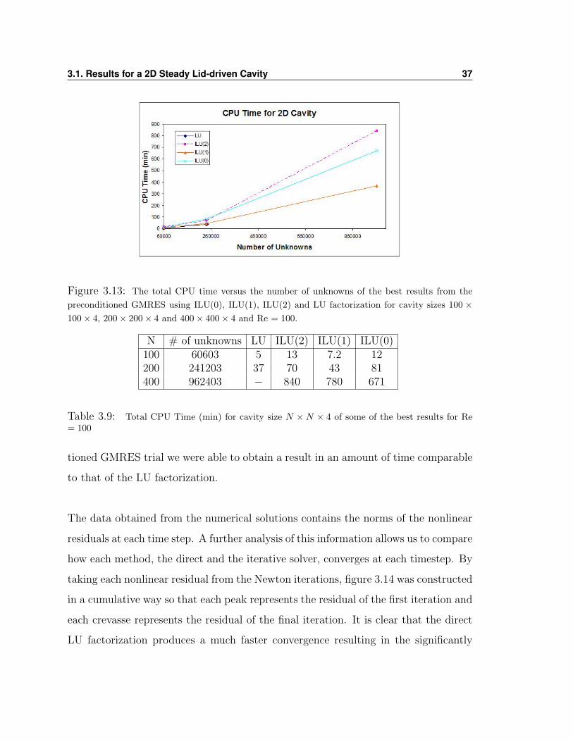
The graph 3.13 shows the total CPU time for some of the best results obtained in this
sectin. Table 3.9 summarizes these CPU times. We can see that for each precondi-
3.1. Results for a 2D Steady Lid-driven Cavity 37
Figure 3.13: The total CPU time versus the number of unknowns of the best results from thepreconditioned GMRES using ILU(0), ILU(1), ILU(2) and LU factorization for cavity sizes 100 ×100× 4, 200× 200× 4 and 400× 400× 4 and Re = 100.
N # of unknowns LU ILU(2) ILU(1) ILU(0)100 60603 5 13 7.2 12200 241203 37 70 43 81400 962403 − 840 780 671
Table 3.9: Total CPU Time (min) for cavity size N × N × 4 of some of the best results for Re= 100
tioned GMRES trial we were able to obtain a result in an amount of time comparable
to that of the LU factorization.
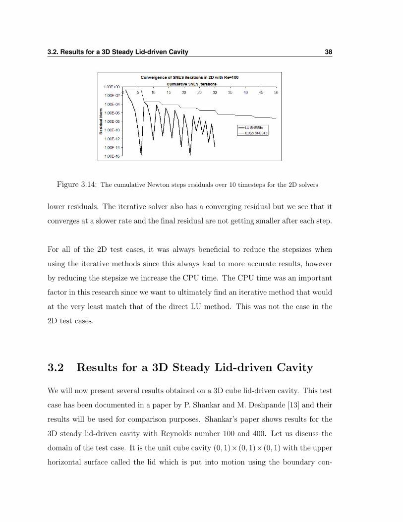
The data obtained from the numerical solutions contains the norms of the nonlinear
residuals at each time step. A further analysis of this information allows us to compare
how each method, the direct and the iterative solver, converges at each timestep. By
taking each nonlinear residual from the Newton iterations, figure 3.14 was constructed
in a cumulative way so that each peak represents the residual of the first iteration and
each crevasse represents the residual of the final iteration. It is clear that the direct
LU factorization produces a much faster convergence resulting in the significantly
3.2. Results for a 3D Steady Lid-driven Cavity 38
Figure 3.14: The cumulative Newton steps residuals over 10 timesteps for the 2D solvers
lower residuals. The iterative solver also has a converging residual but we see that it
converges at a slower rate and the final residual are not getting smaller after each step.
For all of the 2D test cases, it was always beneficial to reduce the stepsizes when
using the iterative methods since this always lead to more accurate results, however
by reducing the stepsize we increase the CPU time. The CPU time was an important
factor in this research since we want to ultimately find an iterative method that would
at the very least match that of the direct LU method. This was not the case in the
2D test cases.
3.2 Results for a 3D Steady Lid-driven Cavity
We will now present several results obtained on a 3D cube lid-driven cavity. This test
case has been documented in a paper by P. Shankar and M. Deshpande [13] and their
results will be used for comparison purposes. Shankar’s paper shows results for the
3D steady lid-driven cavity with Reynolds number 100 and 400. Let us discuss the
domain of the test case. It is the unit cube cavity (0, 1)×(0, 1)×(0, 1) with the upper
horizontal surface called the lid which is put into motion using the boundary con-
3.2. Results for a 3D Steady Lid-driven Cavity 39
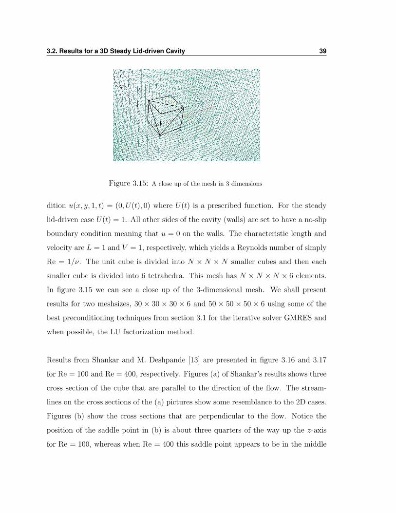
Figure 3.15: A close up of the mesh in 3 dimensions
dition u(x, y, 1, t) = (0, U(t), 0) where U(t) is a prescribed function. For the steady
lid-driven case U(t) = 1. All other sides of the cavity (walls) are set to have a no-slip
boundary condition meaning that u = 0 on the walls. The characteristic length and
velocity are L = 1 and V = 1, respectively, which yields a Reynolds number of simply
Re = 1/ν. The unit cube is divided into N × N × N smaller cubes and then each
smaller cube is divided into 6 tetrahedra. This mesh has N × N × N × 6 elements.
In figure 3.15 we can see a close up of the 3-dimensional mesh. We shall present
results for two meshsizes, 30 × 30 × 30 × 6 and 50 × 50 × 50 × 6 using some of the
best preconditioning techniques from section 3.1 for the iterative solver GMRES and
when possible, the LU factorization method.
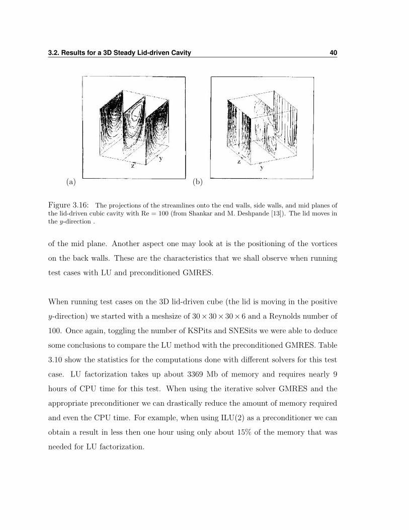
Results from Shankar and M. Deshpande [13] are presented in figure 3.16 and 3.17
for Re = 100 and Re = 400, respectively. Figures (a) of Shankar’s results shows three
cross section of the cube that are parallel to the direction of the flow. The stream-
lines on the cross sections of the (a) pictures show some resemblance to the 2D cases.
Figures (b) show the cross sections that are perpendicular to the flow. Notice the
position of the saddle point in (b) is about three quarters of the way up the z-axis
for Re = 100, whereas when Re = 400 this saddle point appears to be in the middle
3.2. Results for a 3D Steady Lid-driven Cavity 40
(a) (b)
Figure 3.16: The projections of the streamlines onto the end walls, side walls, and mid planes ofthe lid-driven cubic cavity with Re = 100 (from Shankar and M. Deshpande [13]). The lid moves inthe y-direction .
of the mid plane. Another aspect one may look at is the positioning of the vortices
on the back walls. These are the characteristics that we shall observe when running
test cases with LU and preconditioned GMRES.
When running test cases on the 3D lid-driven cube (the lid is moving in the positive
y-direction) we started with a meshsize of 30× 30× 30× 6 and a Reynolds number of
100. Once again, toggling the number of KSPits and SNESits we were able to deduce
some conclusions to compare the LU method with the preconditioned GMRES. Table
3.10 show the statistics for the computations done with different solvers for this test
case. LU factorization takes up about 3369 Mb of memory and requires nearly 9
hours of CPU time for this test. When using the iterative solver GMRES and the
appropriate preconditioner we can drastically reduce the amount of memory required
and even the CPU time. For example, when using ILU(2) as a preconditioner we can
obtain a result in less then one hour using only about 15% of the memory that was
needed for LU factorization.
3.2. Results for a 3D Steady Lid-driven Cavity 41
(a) (b)
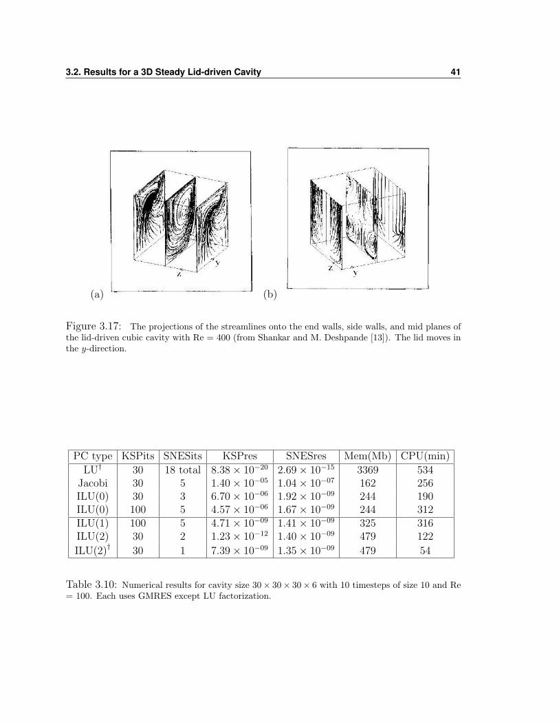
Figure 3.17: The projections of the streamlines onto the end walls, side walls, and mid planes ofthe lid-driven cubic cavity with Re = 400 (from Shankar and M. Deshpande [13]). The lid moves inthe y-direction.
PC type KSPits SNESits KSPres SNESres Mem(Mb) CPU(min)
LU† 30 18 total 8.38× 10⁻²⁰ 2.69× 10⁻¹⁵ 3369 534Jacobi 30 5 1.40× 10−05 1.04× 10−07 162 256ILU(0) 30 3 6.70× 10−06 1.92× 10−09 244 190ILU(0) 100 5 4.57× 10−06 1.67× 10−09 244 312ILU(1) 100 5 4.71× 10−09 1.41× 10−09 325 316ILU(2) 30 2 1.23× 10⁻¹² 1.40× 10−09 479 122
ILU(2)† 30 1 7.39× 10−09 1.35× 10−09 479 54
Table 3.10: Numerical results for cavity size 30× 30× 30× 6 with 10 timesteps of size 10 and Re= 100. Each uses GMRES except LU factorization.
3.2. Results for a 3D Steady Lid-driven Cavity 42
(a) (b)
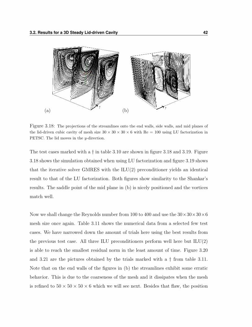
Figure 3.18: The projections of the streamlines onto the end walls, side walls, and mid planes ofthe lid-driven cubic cavity of mesh size 30 × 30 × 30 × 6 with Re = 100 using LU factorization inPETSC. The lid moves in the y-direction.
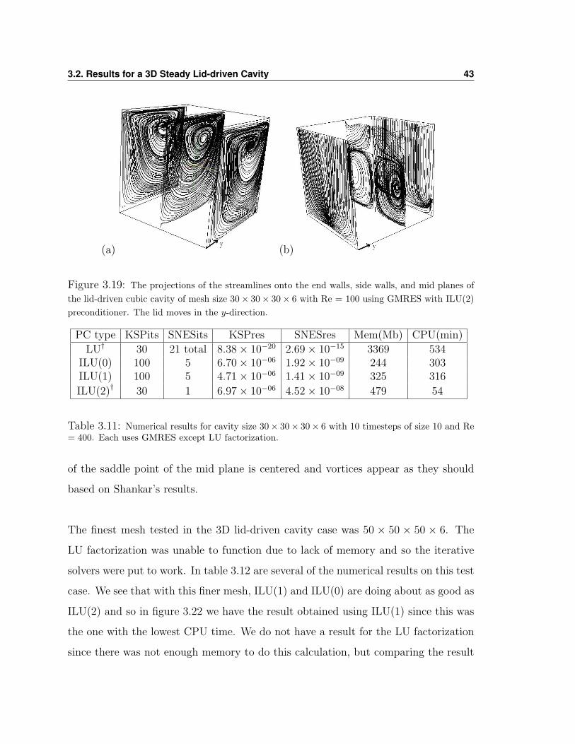
The test cases marked with a † in table 3.10 are shown in figure 3.18 and 3.19. Figure
3.18 shows the simulation obtained when using LU factorization and figure 3.19 shows
that the iterative solver GMRES with the ILU(2) preconditioner yields an identical
result to that of the LU factorization. Both figures show similarity to the Shankar’s
results. The saddle point of the mid plane in (b) is nicely positioned and the vortices
match well.
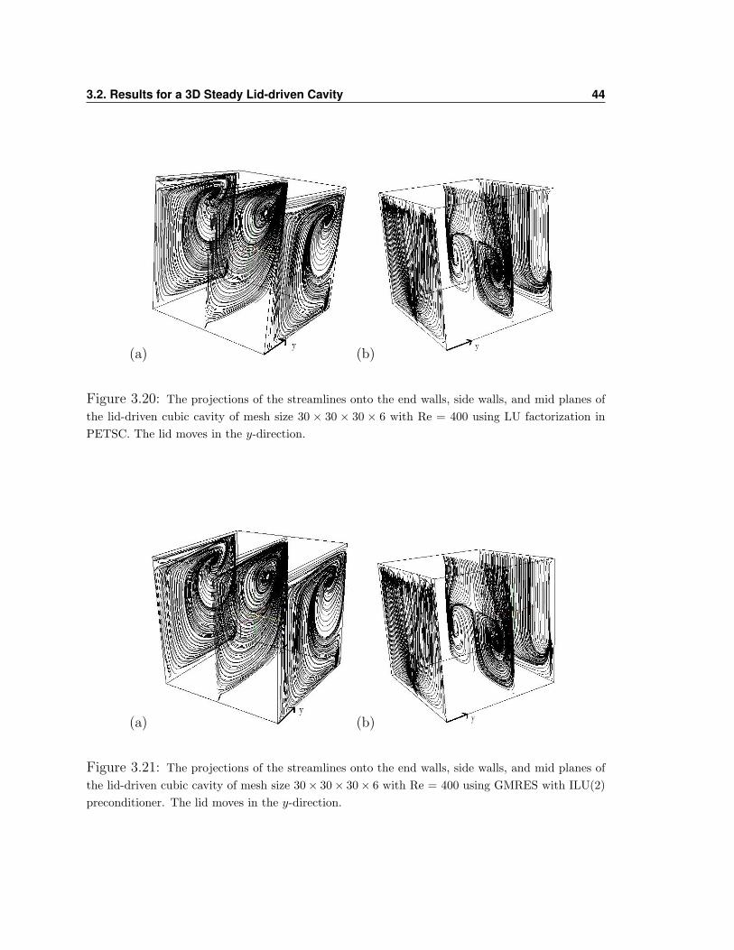
Now we shall change the Reynolds number from 100 to 400 and use the 30×30×30×6
mesh size once again. Table 3.11 shows the numerical data from a selected few test
cases. We have narrowed down the amount of trials here using the best results from
the previous test case. All three ILU preconditioners perform well here but ILU(2)
is able to reach the smallest residual norm in the least amount of time. Figure 3.20
and 3.21 are the pictures obtained by the trials marked with a † from table 3.11.
Note that on the end walls of the figures in (b) the streamlines exhibit some erratic
behavior. This is due to the coarseness of the mesh and it dissipates when the mesh
is refined to 50× 50× 50× 6 which we will see next. Besides that flaw, the position
3.2. Results for a 3D Steady Lid-driven Cavity 43
(a) (b)
Figure 3.19: The projections of the streamlines onto the end walls, side walls, and mid planes ofthe lid-driven cubic cavity of mesh size 30× 30× 30× 6 with Re = 100 using GMRES with ILU(2)preconditioner. The lid moves in the y-direction.
PC type KSPits SNESits KSPres SNESres Mem(Mb) CPU(min)
LU† 30 21 total 8.38× 10⁻²⁰ 2.69× 10⁻¹⁵ 3369 534ILU(0) 100 5 6.70× 10−06 1.92× 10−09 244 303ILU(1) 100 5 4.71× 10−06 1.41× 10−09 325 316
ILU(2)† 30 1 6.97× 10−06 4.52× 10−08 479 54
Table 3.11: Numerical results for cavity size 30× 30× 30× 6 with 10 timesteps of size 10 and Re= 400. Each uses GMRES except LU factorization.
of the saddle point of the mid plane is centered and vortices appear as they should
based on Shankar’s results.
The finest mesh tested in the 3D lid-driven cavity case was 50 × 50 × 50 × 6. The
LU factorization was unable to function due to lack of memory and so the iterative
solvers were put to work. In table 3.12 are several of the numerical results on this test
case. We see that with this finer mesh, ILU(1) and ILU(0) are doing about as good as
ILU(2) and so in figure 3.22 we have the result obtained using ILU(1) since this was
the one with the lowest CPU time. We do not have a result for the LU factorization
since there was not enough memory to do this calculation, but comparing the result
3.2. Results for a 3D Steady Lid-driven Cavity 44
(a) (b)
Figure 3.20: The projections of the streamlines onto the end walls, side walls, and mid planes ofthe lid-driven cubic cavity of mesh size 30 × 30 × 30 × 6 with Re = 400 using LU factorization inPETSC. The lid moves in the y-direction.
(a) (b)
Figure 3.21: The projections of the streamlines onto the end walls, side walls, and mid planes ofthe lid-driven cubic cavity of mesh size 30× 30× 30× 6 with Re = 400 using GMRES with ILU(2)preconditioner. The lid moves in the y-direction.
3.2. Results for a 3D Steady Lid-driven Cavity 45
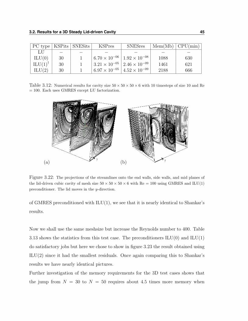
PC type KSPits SNESits KSPres SNESres Mem(Mb) CPU(min)LU − − − − − −
ILU(0) 30 1 6.70× 10−06 1.92× 10−08 1088 630
ILU(1)† 30 1 3.21× 10−05 2.46× 10−09 1461 621ILU(2) 30 1 6.97× 10−05 4.52× 10−09 2188 666
Table 3.12: Numerical results for cavity size 50× 50× 50× 6 with 10 timesteps of size 10 and Re= 100. Each uses GMRES except LU factorization.
(a) (b)
Figure 3.22: The projections of the streamlines onto the end walls, side walls, and mid planes ofthe lid-driven cubic cavity of mesh size 50× 50× 50× 6 with Re = 100 using GMRES and ILU(1)preconditioner. The lid moves in the y-direction.
of GMRES preconditioned with ILU(1), we see that it is nearly identical to Shankar’s
results.
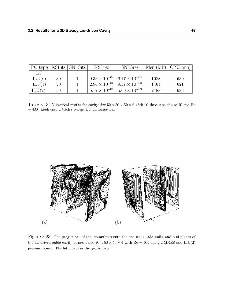
Now we shall use the same meshsize but increase the Reynolds number to 400. Table
3.13 shows the statistics from this test case. The preconditioners ILU(0) and ILU(1)
do satisfactory jobs but here we chose to show in figure 3.23 the result obtained using
ILU(2) since it had the smallest residuals. Once again comparing this to Shankar’s
results we have nearly identical pictures.
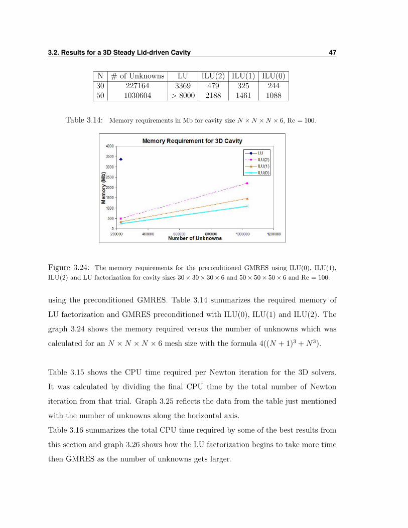
Further investigation of the memory requirements for the 3D test cases shows that
the jump from N = 30 to N = 50 requires about 4.5 times more memory when
3.2. Results for a 3D Steady Lid-driven Cavity 46
PC type KSPits SNESits KSPres SNESres Mem(Mb) CPU(min)LU − − − − − −
ILU(0) 30 1 9.33× 10−04 6.17× 10−08 1088 630ILU(1) 30 1 2.96× 10−05 9.37× 10−08 1461 621
ILU(2)† 30 1 5.12× 10−05 5.06× 10−09 2188 683
Table 3.13: Numerical results for cavity size 50× 50× 50× 6 with 10 timesteps of size 10 and Re= 400. Each uses GMRES except LU factorization.
(a) (b)
Figure 3.23: The projections of the streamlines onto the end walls, side walls, and mid planes ofthe lid-driven cubic cavity of mesh size 50× 50× 50× 6 with Re = 400 using GMRES and ILU(2)preconditioner. The lid moves in the y-direction.
3.2. Results for a 3D Steady Lid-driven Cavity 47
N # of Unknowns LU ILU(2) ILU(1) ILU(0)30 227164 3369 479 325 24450 1030604 > 8000 2188 1461 1088
Table 3.14: Memory requirements in Mb for cavity size N ×N ×N × 6, Re = 100.
Figure 3.24: The memory requirements for the preconditioned GMRES using ILU(0), ILU(1),ILU(2) and LU factorization for cavity sizes 30× 30× 30× 6 and 50× 50× 50× 6 and Re = 100.
using the preconditioned GMRES. Table 3.14 summarizes the required memory of
LU factorization and GMRES preconditioned with ILU(0), ILU(1) and ILU(2). The
graph 3.24 shows the memory required versus the number of unknowns which was
calculated for an N ×N ×N × 6 mesh size with the formula 4((N + 1)3 +N3).
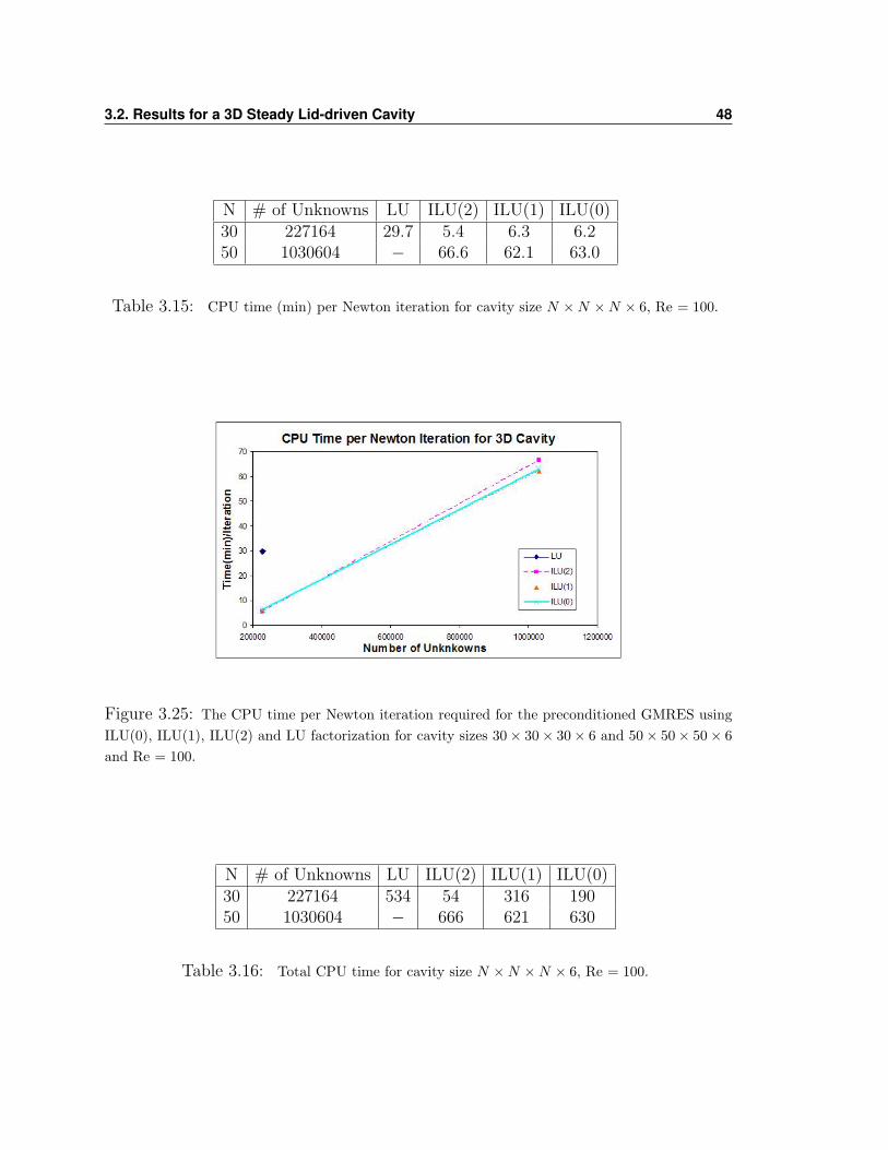
Table 3.15 shows the CPU time required per Newton iteration for the 3D solvers.
It was calculated by dividing the final CPU time by the total number of Newton
iteration from that trial. Graph 3.25 reflects the data from the table just mentioned
with the number of unknowns along the horizontal axis.
Table 3.16 summarizes the total CPU time required by some of the best results from
this section and graph 3.26 shows how the LU factorization begins to take more time
then GMRES as the number of unknowns gets larger.
3.2. Results for a 3D Steady Lid-driven Cavity 48
N # of Unknowns LU ILU(2) ILU(1) ILU(0)30 227164 29.7 5.4 6.3 6.250 1030604 − 66.6 62.1 63.0
Table 3.15: CPU time (min) per Newton iteration for cavity size N ×N ×N × 6, Re = 100.
Figure 3.25: The CPU time per Newton iteration required for the preconditioned GMRES usingILU(0), ILU(1), ILU(2) and LU factorization for cavity sizes 30× 30× 30× 6 and 50× 50× 50× 6and Re = 100.
N # of Unknowns LU ILU(2) ILU(1) ILU(0)30 227164 534 54 316 19050 1030604 − 666 621 630
Table 3.16: Total CPU time for cavity size N ×N ×N × 6, Re = 100.
3.3. Results for a 2D Pulsating Lid-driven Cavity 49
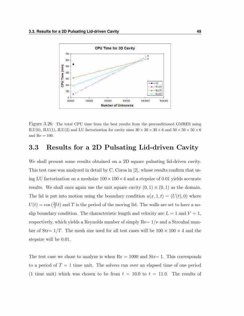
Figure 3.26: The total CPU time from the best results from the preconditioned GMRES usingILU(0), ILU(1), ILU(2) and LU factorization for cavity sizes 30× 30× 30× 6 and 50× 50× 50× 6and Re = 100.
3.3 Results for a 2D Pulsating Lid-driven Cavity
We shall present some results obtained on a 2D square pulsating lid-driven cavity.
This test case was analyzed in detail by C. Coros in [2], whose results confirm that us-
ing LU factorization on a meshsize 100×100×4 and a stepsize of 0.01 yields accurate
results. We shall once again use the unit square cavity (0, 1)× (0, 1) as the domain.
The lid is put into motion using the boundary condition u(x, 1, t) = (U(t), 0) where
U(t) = cos (2πTt) and T is the period of the moving lid. The walls are set to have a no-
slip boundary condition. The characteristic length and velocity are L = 1 and V = 1,
respectively, which yields a Reynolds number of simply Re= 1/ν and a Strouhal num-
ber of Str= 1/T . The mesh size used for all test cases will be 100× 100× 4 and the
stepsize will be 0.01.
The test case we chose to analyze is when Re = 1000 and Str= 1. This corresponds
to a period of T = 1 time unit. The solvers run over an elapsed time of one period
(1 time unit) which was chosen to be from t = 10.0 to t = 11.0. The results of
3.3. Results for a 2D Pulsating Lid-driven Cavity 50
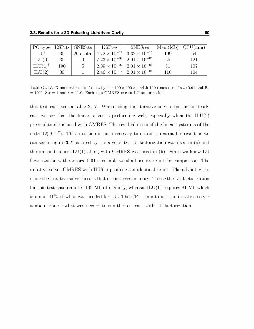
PC type KSPits SNESits KSPres SNESres Mem(Mb) CPU(min)
LU† 30 205 total 4.72× 10⁻¹⁹ 3.32× 10⁻¹² 199 54ILU(0) 30 10 7.23× 10−07 2.01× 10−02 65 121
ILU(1)† 100 5 2.09× 10−07 2.01× 10−02 81 107ILU(2) 30 1 2.46× 10⁻¹⁷ 2.01× 10−02 110 104
Table 3.17: Numerical results for cavity size 100× 100× 4 with 100 timesteps of size 0.01 and Re= 1000, Str = 1 and t = 11.0. Each uses GMRES except LU factorization.
this test case are in table 3.17. When using the iterative solvers on the unsteady
case we see that the linear solver is performing well, especially when the ILU(2)
preconditioner is used with GMRES. The residual norm of the linear system is of the
order O(10−17). This precision is not necessary to obtain a reasonable result as we
can see in figure 3.27,colored by the y velocity. LU factorization was used in (a) and
the preconditioner ILU(1) along with GMRES was used in (b). Since we know LU
factorization with stepsize 0.01 is reliable we shall use its result for comparison. The
iterative solver GMRES with ILU(1) produces an identical result. The advantage to
using the iterative solver here is that it conserves memory. To use the LU factorization
for this test case requires 199 Mb of memory, whereas ILU(1) requires 81 Mb which
is about 41% of what was needed for LU. The CPU time to use the iterative solver
is about double what was needed to run the test case with LU factorization.
3.3. Results for a 2D Pulsating Lid-driven Cavity 51
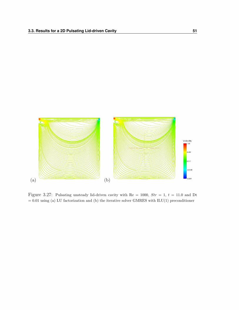
(a) (b)
Figure 3.27: Pulsating unsteady lid-driven cavity with Re = 1000, Str = 1, t = 11.0 and Dt= 0.01 using (a) LU factorization and (b) the iterative solver GMRES with ILU(1) preconditioner
Chapter 4
Adaptive Time Stepping
4.1 Outline of the Method
Adaptive time stepping methods are used to control the discretization error by con-
trolling the size of the time steps. The use of smaller timestep sizes results in more
accurate results but at the cost of larger CPU times. One solution to optimize this
compromise would be to derive a method that uses a timestep size that is re-calculated
after each timestep to make the proper adjustments. This could ideally be more ef-
fective in solving our Navier–Stokes problem. There is a method proposed in [6] for
a TR-BDF2 (TR for trapezoidal rule) adaptive time stepping scheme where TR is
used for the first step, a “leapfrog” method is used to predict the velocity and then
adaptive-BDF2 is used with the predictor as its first guess. To keep consistency within
the code that was used to implement the constant stepsize test cases from Chapter 3,
I have modified Gresho’s proposed scheme to use a BE startup, the leapfrog predictor
and then adaptive-BDF2 for the remaining steps.
52
4.1. Outline of the Method 53
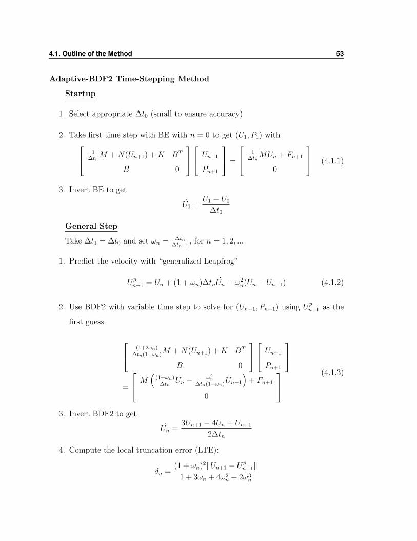
Adaptive-BDF2 Time-Stepping Method
Startup
1. Select appropriate ∆t0 (small to ensure accuracy)
2. Take first time step with BE with n = 0 to get (U1, P1) with 1∆tn
M +N(Un+1) +K BT
B 0
Un+1
Pn+1
=
1∆tn
MUn + Fn+1
0
(4.1.1)
3. Invert BE to get
U1 =U1 − U0
∆t0
General Step
Take ∆t1 = ∆t0 and set ωn = ∆tn∆tn−1
, for n = 1, 2, ...
1. Predict the velocity with “generalized Leapfrog”
Upn+1 = Un + (1 + ωn)∆tnUn − ω2
n(Un − Un−1) (4.1.2)
2. Use BDF2 with variable time step to solve for (Un+1, Pn+1) using Upn+1 as the
first guess.
(1+2ωn)∆tn(1+ωn)
M +N(Un+1) +K BT
B 0
Un+1
Pn+1
=
M(
(1+ωn)∆tn
Un − ω2n
∆tn(1+ωn)Un−1
)+ Fn+1
0
(4.1.3)
3. Invert BDF2 to get
Un =3Un+1 − 4Un + Un−1
2∆tn
4. Compute the local truncation error (LTE):
dn =(1 + ωn)2‖Un+1 − Up
n+1‖1 + 3ωn + 4ω2
n + 2ω3n
4.2. Results of Adaptive Time Stepping on the 2D Lid-driven Cavity 54
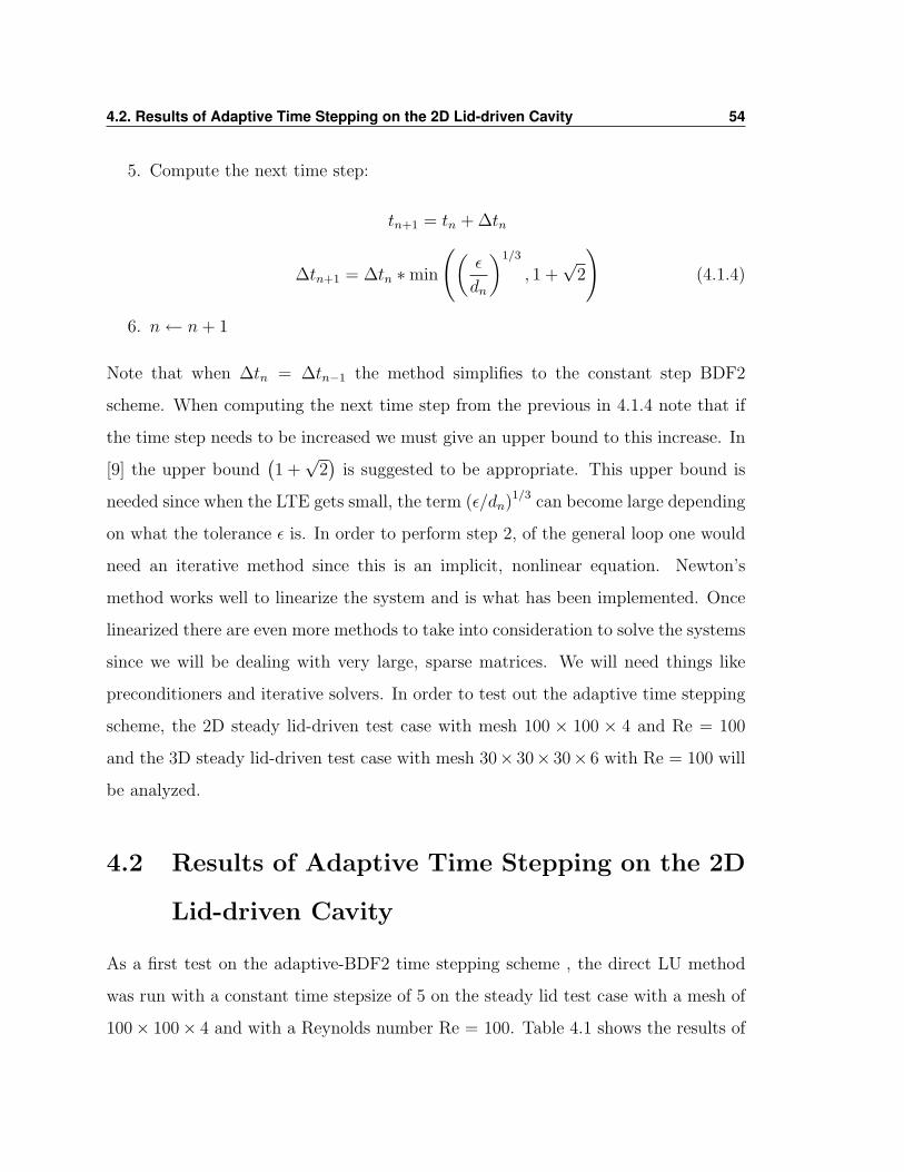
5. Compute the next time step:
tn+1 = tn + ∆tn
∆tn+1 = ∆tn ∗min
((ε
dn
)1/3
, 1 +√
2
)(4.1.4)
6. n← n+ 1
Note that when ∆tn = ∆tn−1 the method simplifies to the constant step BDF2
scheme. When computing the next time step from the previous in 4.1.4 note that if
the time step needs to be increased we must give an upper bound to this increase. In
[9] the upper bound(1 +√
2)
is suggested to be appropriate. This upper bound is
needed since when the LTE gets small, the term (ε/dn)1/3 can become large depending
on what the tolerance ε is. In order to perform step 2, of the general loop one would
need an iterative method since this is an implicit, nonlinear equation. Newton’s
method works well to linearize the system and is what has been implemented. Once
linearized there are even more methods to take into consideration to solve the systems
since we will be dealing with very large, sparse matrices. We will need things like
preconditioners and iterative solvers. In order to test out the adaptive time stepping
scheme, the 2D steady lid-driven test case with mesh 100 × 100 × 4 and Re = 100
and the 3D steady lid-driven test case with mesh 30× 30× 30× 6 with Re = 100 will
be analyzed.
4.2 Results of Adaptive Time Stepping on the 2D
Lid-driven Cavity
As a first test on the adaptive-BDF2 time stepping scheme , the direct LU method
was run with a constant time stepsize of 5 on the steady lid test case with a mesh of
100× 100× 4 and with a Reynolds number Re = 100. Table 4.1 shows the results of
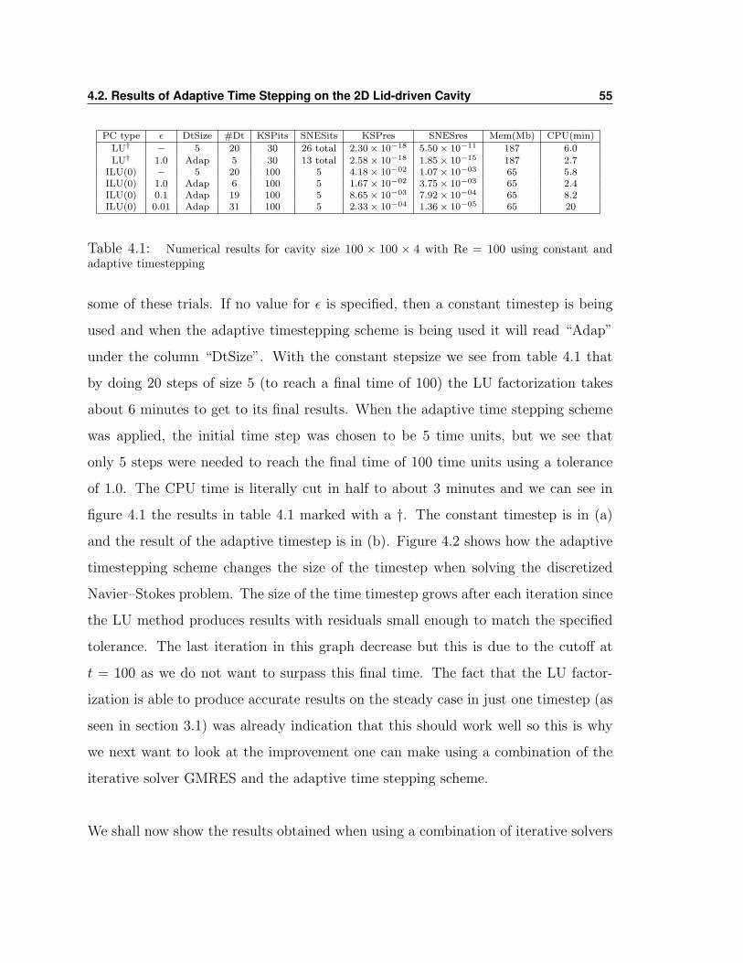
4.2. Results of Adaptive Time Stepping on the 2D Lid-driven Cavity 55
PC type ε DtSize #Dt KSPits SNESits KSPres SNESres Mem(Mb) CPU(min)
LU† − 5 20 30 26 total 2.30× 10⁻¹⁸ 5.50× 10⁻¹¹ 187 6.0
LU† 1.0 Adap 5 30 13 total 2.58× 10⁻¹⁸ 1.85× 10⁻¹⁵ 187 2.7ILU(0) − 5 20 100 5 4.18× 10−02 1.07× 10−03 65 5.8ILU(0) 1.0 Adap 6 100 5 1.67× 10−02 3.75× 10−03 65 2.4ILU(0) 0.1 Adap 19 100 5 8.65× 10−03 7.92× 10−04 65 8.2ILU(0) 0.01 Adap 31 100 5 2.33× 10−04 1.36× 10−05 65 20
Table 4.1: Numerical results for cavity size 100 × 100 × 4 with Re = 100 using constant andadaptive timestepping
some of these trials. If no value for ε is specified, then a constant timestep is being
used and when the adaptive timestepping scheme is being used it will read “Adap”
under the column “DtSize”. With the constant stepsize we see from table 4.1 that
by doing 20 steps of size 5 (to reach a final time of 100) the LU factorization takes
about 6 minutes to get to its final results. When the adaptive time stepping scheme
was applied, the initial time step was chosen to be 5 time units, but we see that
only 5 steps were needed to reach the final time of 100 time units using a tolerance
of 1.0. The CPU time is literally cut in half to about 3 minutes and we can see in
figure 4.1 the results in table 4.1 marked with a †. The constant timestep is in (a)
and the result of the adaptive timestep is in (b). Figure 4.2 shows how the adaptive
timestepping scheme changes the size of the timestep when solving the discretized
Navier–Stokes problem. The size of the time timestep grows after each iteration since
the LU method produces results with residuals small enough to match the specified
tolerance. The last iteration in this graph decrease but this is due to the cutoff at
t = 100 as we do not want to surpass this final time. The fact that the LU factor-
ization is able to produce accurate results on the steady case in just one timestep (as
seen in section 3.1) was already indication that this should work well so this is why
we next want to look at the improvement one can make using a combination of the
iterative solver GMRES and the adaptive time stepping scheme.
We shall now show the results obtained when using a combination of iterative solvers
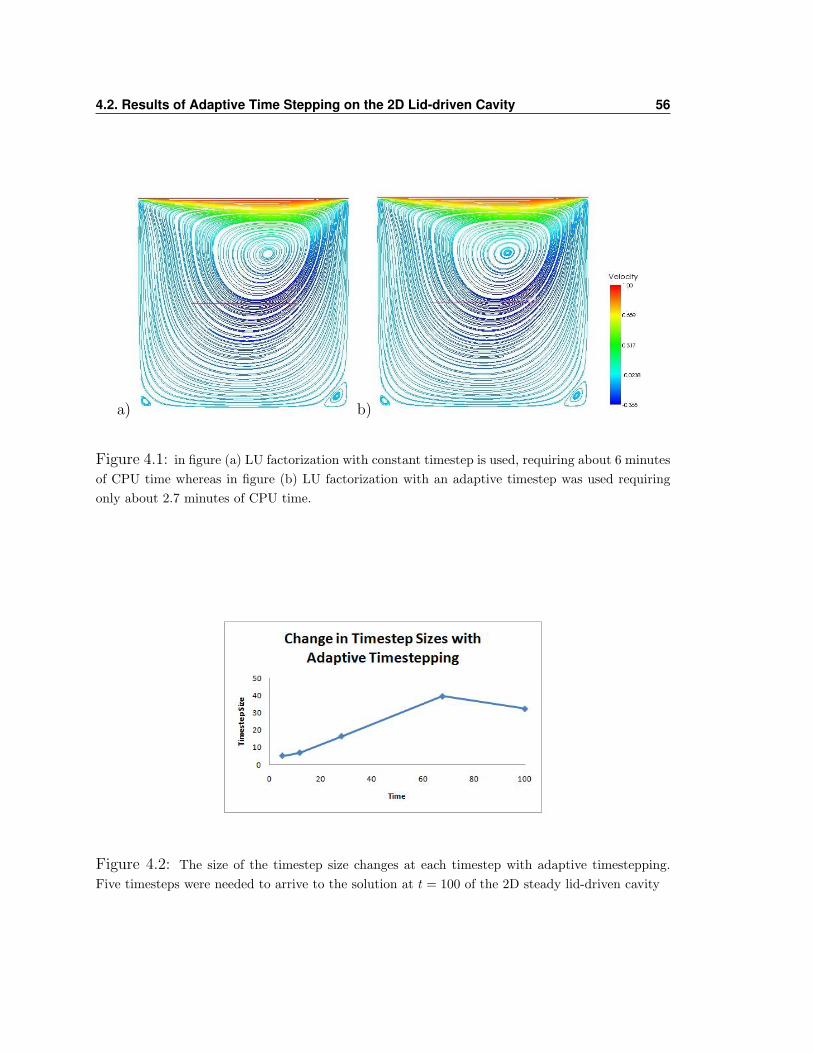
4.2. Results of Adaptive Time Stepping on the 2D Lid-driven Cavity 56
a) b)
Figure 4.1: in figure (a) LU factorization with constant timestep is used, requiring about 6 minutesof CPU time whereas in figure (b) LU factorization with an adaptive timestep was used requiringonly about 2.7 minutes of CPU time.
Figure 4.2: The size of the timestep size changes at each timestep with adaptive timestepping.Five timesteps were needed to arrive to the solution at t = 100 of the 2D steady lid-driven cavity
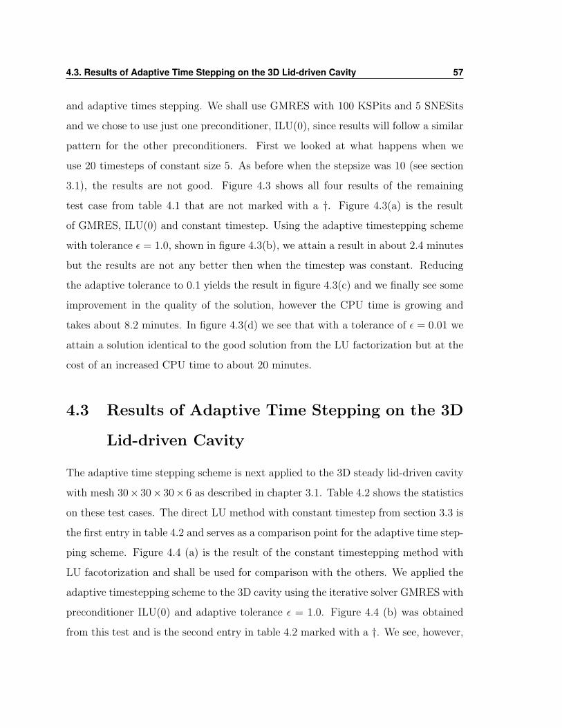
4.3. Results of Adaptive Time Stepping on the 3D Lid-driven Cavity 57
and adaptive times stepping. We shall use GMRES with 100 KSPits and 5 SNESits
and we chose to use just one preconditioner, ILU(0), since results will follow a similar
pattern for the other preconditioners. First we looked at what happens when we
use 20 timesteps of constant size 5. As before when the stepsize was 10 (see section
3.1), the results are not good. Figure 4.3 shows all four results of the remaining
test case from table 4.1 that are not marked with a †. Figure 4.3(a) is the result
of GMRES, ILU(0) and constant timestep. Using the adaptive timestepping scheme
with tolerance ε = 1.0, shown in figure 4.3(b), we attain a result in about 2.4 minutes
but the results are not any better then when the timestep was constant. Reducing
the adaptive tolerance to 0.1 yields the result in figure 4.3(c) and we finally see some
improvement in the quality of the solution, however the CPU time is growing and
takes about 8.2 minutes. In figure 4.3(d) we see that with a tolerance of ε = 0.01 we
attain a solution identical to the good solution from the LU factorization but at the
cost of an increased CPU time to about 20 minutes.
4.3 Results of Adaptive Time Stepping on the 3D
Lid-driven Cavity
The adaptive time stepping scheme is next applied to the 3D steady lid-driven cavity
with mesh 30× 30× 30× 6 as described in chapter 3.1. Table 4.2 shows the statistics
on these test cases. The direct LU method with constant timestep from section 3.3 is
the first entry in table 4.2 and serves as a comparison point for the adaptive time step-
ping scheme. Figure 4.4 (a) is the result of the constant timestepping method with
LU facotorization and shall be used for comparison with the others. We applied the
adaptive timestepping scheme to the 3D cavity using the iterative solver GMRES with
preconditioner ILU(0) and adaptive tolerance ε = 1.0. Figure 4.4 (b) was obtained
from this test and is the second entry in table 4.2 marked with a †. We see, however,
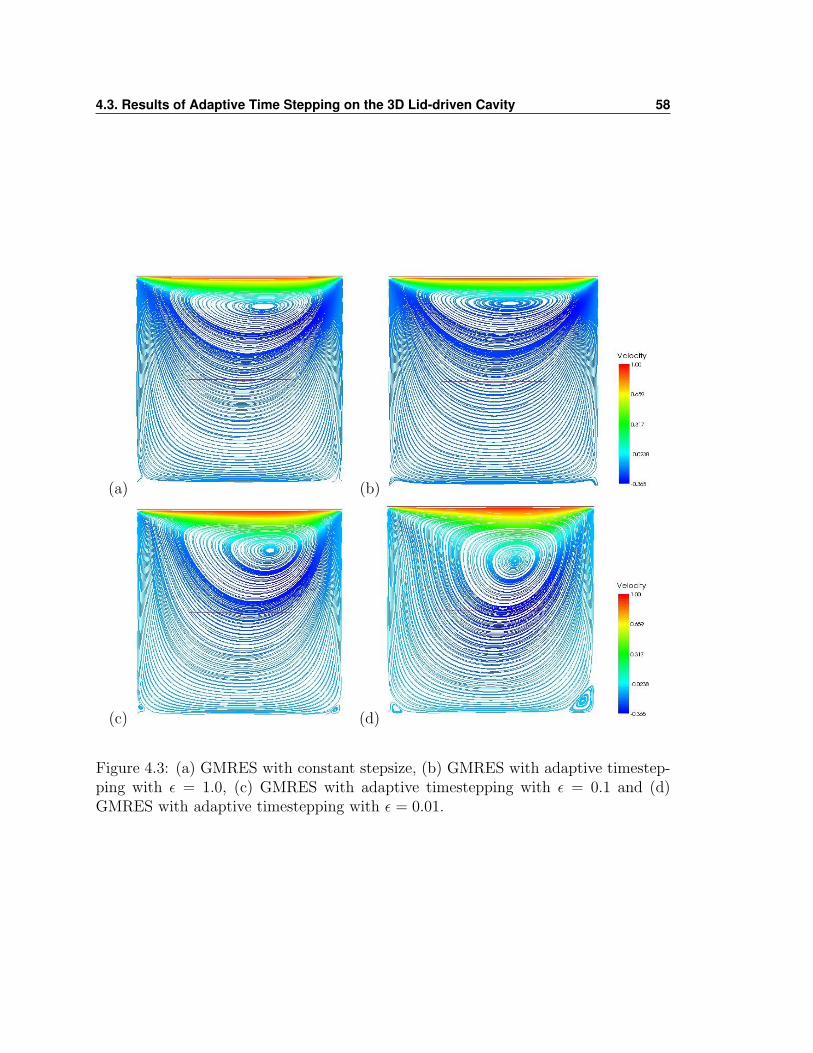
4.3. Results of Adaptive Time Stepping on the 3D Lid-driven Cavity 58
(a) (b)
(c) (d)
Figure 4.3: (a) GMRES with constant stepsize, (b) GMRES with adaptive timestep-ping with ε = 1.0, (c) GMRES with adaptive timestepping with ε = 0.1 and (d)GMRES with adaptive timestepping with ε = 0.01.
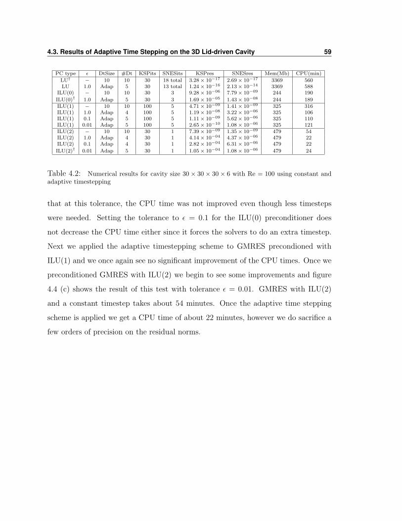
4.3. Results of Adaptive Time Stepping on the 3D Lid-driven Cavity 59
PC type ε DtSize #Dt KSPits SNESits KSPres SNESres Mem(Mb) CPU(min)
LU† − 10 10 30 18 total 3.28× 10⁻¹⁷ 2.69× 10⁻¹⁷ 3369 560LU 1.0 Adap 5 30 13 total 1.24× 10⁻¹⁶ 2.13× 10⁻¹⁴ 3369 588
ILU(0) − 10 10 30 3 9.28× 10−06 7.79× 10−09 244 190
ILU(0)† 1.0 Adap 5 30 3 1.69× 10−05 1.43× 10−08 244 189ILU(1) − 10 10 100 5 4.71× 10−09 1.41× 10−09 325 316ILU(1) 1.0 Adap 4 100 5 1.19× 10−08 3.22× 10−06 325 106ILU(1) 0.1 Adap 5 100 5 1.11× 10−09 5.62× 10−06 325 110ILU(1) 0.01 Adap 5 100 5 2.65× 10⁻¹⁰ 1.08× 10−06 325 121ILU(2) − 10 10 30 1 7.39× 10−09 1.35× 10−09 479 54ILU(2) 1.0 Adap 4 30 1 4.14× 10−04 4.37× 10−06 479 22ILU(2) 0.1 Adap 4 30 1 2.82× 10−04 6.31× 10−06 479 22
ILU(2)† 0.01 Adap 5 30 1 1.05× 10−04 1.08× 10−06 479 24
Table 4.2: Numerical results for cavity size 30 × 30 × 30 × 6 with Re = 100 using constant andadaptive timestepping
that at this tolerance, the CPU time was not improved even though less timesteps
were needed. Setting the tolerance to ε = 0.1 for the ILU(0) preconditioner does
not decrease the CPU time either since it forces the solvers to do an extra timestep.
Next we applied the adaptive timestepping scheme to GMRES precondioned with
ILU(1) and we once again see no significant improvement of the CPU times. Once we
preconditioned GMRES with ILU(2) we begin to see some improvements and figure
4.4 (c) shows the result of this test with tolerance ε = 0.01. GMRES with ILU(2)
and a constant timestep takes about 54 minutes. Once the adaptive time stepping
scheme is applied we get a CPU time of about 22 minutes, however we do sacrifice a
few orders of precision on the residual norms.
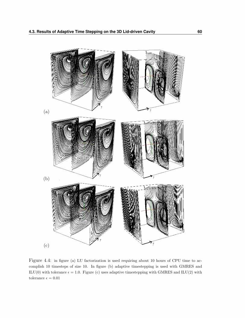
4.3. Results of Adaptive Time Stepping on the 3D Lid-driven Cavity 60
(a)
(b)
(c)
Figure 4.4: in figure (a) LU factorization is used requiring about 10 hours of CPU time to ac-complish 10 timesteps of size 10. In figure (b) adaptive timestepping is used with GMRES andILU(0) with tolerance ε = 1.0. Figure (c) uses adaptive timestepping with GMRES and ILU(2) withtolerance ε = 0.01
Chapter 5
Conclusions
Using iterative methods such as GMRES for solving the discretized Navier–Stokes
equations clearly has its advantages as well as disadvantages. Several test cases were
tried in this thesis in order to outline the characteristics of the direct solver LU fac-
torization and the iterative solver GMRES.
We started out in 2D with a steady lid-driven square cavity and discovered that the
iterative solver GMRES required many iterations in order to achieve a comparable
accuracy to that of the direct LU factorization. The need for additional iterations for
both the linear and nonlinear solvers resulted in an increased CPU time, but overall
it is possible to achieve reasonable results using only a few more minutes than LU
factorization if one is willing to sacrifice a few orders on the nonlinear residual norms.
The benefit of the iterative solver clearly comes from the lower memory requirements,
since running the preconditioned GMRES always required less megabytes than LU.
We tried the 3D steady lid-driven cavity and obtained very positive results. The
CPU times and the memory requirement were cut dramatically and we now see the
benefit of using the iterative solver GMRES on a flow problem. In 3D, direct methods
61
62
are less competitive because larger bandwidths in the sparsity pattern causes more
nonzero elements to be created during the LU factorization. Iterative methods avoid
such problems and are more efficient relative to the direct solver. We did sacrifice a
few orders of precision on the residual norms by using the iterative solve but we see
once the simulations were analyzed graphically that GMRES is just as good (if not
better since it requires much less memory and CPU time) as the traditional direct
method when solving the problem in 3D.
The iterative method GMRES was applied to the 2D unsteady lid-driven cavity and
the best results using the preconditioners ILU(0), ILU(1) and ILU(2) were applied to
this oscillating problem. As previously discovered about GMRES on the 2D problem,
it can conserve memory but not always CPU time. Using ILU(0) as a preconditioner
for this problem, one can obtain a very comparable solution to that of LU factoriza-
tion due to the efficiency of the linear solver in this case.
In an attempt to eliminate the need to self-choose the size of the timestep required,
an adaptive BDF2 timestepping scheme was implemented. It was tested on both the
2D ad 3D steady lid-driven cavities. Applying this adaptive time stepping scheme to
the LU factorization method we were able to see the efficiency of the method. Given
the size of the initial timestep, adaptive BDF2 will start increasing the stepsize right
away (recall that LU factorization can solve the 2D steady-lid driven problem in just
1 timestep). It was more interesting to see what the effects were on the iterative
solvers. In 2D we found that with ILU(0) preconditioner we could arrive to the same
accuracy as was achieved with the constant timestepping in about half the time. We
can then decrease the tolerance of the adaptive solver to achieve more precision but
this resulted in more timesteps and hence higher CPU time. The CPU time of the
most accurate results surpassed that of the LU factorization. We then applied the
adaptive BDF2 to the 3D steady-lid driven problem. The results were positive as was

63
the case with the steady lid-driven cavity in 3D. We were successfully able to reduce
the CPU time of the already fast iterative solver GMRES and maintain about the
same accuracy.
Bibliography
[1] S. Balay, K. Buschelman, and more... PetSc User’s Manual, Argonne National
Laboratory, Argonne, 2007.
[2] C. Coros, Y. Bourgault , On the numerical study of periodically forced
2-D cavity flows International Journal for Numerical Methods in Fluids, Int.
J. Numer. Meth. Fluids, Submitted.
[3] R. L. Devaney, An Introduction to Chaotic Dynamical Systems, The
Benjamin/Cummings Publ. Co., 1986.
[4] A. Ern and J.-L. Guermond, Theory and Practice of Finite Elements,
Applied Mathematical Sciences, Springer, 2005.
[5] U. Ghia, N. Ghia, C. Shin, High-Re Solutions for Incompressible Flow
Using the Navier-Stokes Equations and a Multigrid Method, Journal of
Computational Physics 48, 387-411, 1982.
[6] P. Gresho, D. Griffiths and D. Sylvester, Adaptive Time-Stepping for In-
compressible Flow Part I: Scalar Advection-Diffusion, Society for Indus-
trial and Applied Mathematics, SIAM Journal of Scientific Computations , Vol.
30, No. 4, pp. 2018-2054, 2008.
64
BIBLIOGRAPHY 65
[7] P. Gresho and R. Sani, Incompressible Flow and the Finite Element
Method, Volume 2: Isothermal Laminar Flow, John Wiley and sons,
Ltd., 2000.
[8] E. Hairer, S.P. Norsett and G. Wanner, Solving Ordinary Differential Equa-
tions I, Second Revised Edition, Springer-Verlag, Berlin Heidelberg, 1993.
[9] E. Hairer and G. Wanner, Solving Ordinary Differential Equations II, Stiff
and Differential-Algebraic Problems, Springer-Verlag, Berlin Heidelberg, 1991.
[10] Iwatsu R, Ishii K, Kawamura T, Kuwahara K,Hyun JM. Simulation of tran-
sition to turbulence in a cubic cavity. AIAA Pap. No. 98-0040, 1989.
[11] P. Kjellgren, A semi-implicit fractional step finite element method for
viscous incompressible flows, Computational Mechanics 20: 541-550, 1997.
[12] Y. Saad, Iterative methods for sparse linear systems , Societey for Indus-
trial and Applied Mathematics (SIAM), 2007.
[13] P. N. Shankar and M. D. Deshpande, Fluid Mechanics in the Driven Cavity
Annu. Rev. Fluid Mech., 32:93136, 2000.


